Preferences for Truth-telling

Johannes Abeler, Daniele Nosenzo and Collin Raymond∗

August 8, 2017

Abstract

Private information is at the heart of many economic activities. For decades, economists

have assumed that individuals are willing to misreport private information if this maxi-

mizes their material payoff. We combine data from 90 experimental studies in economics,

psychology and sociology, and show that, in fact, people lie surprisingly little. We then for-

malize a wide range of potential explanations for the observed behavior, identify testable

predictions that can distinguish between the models and conduct new experiments to do

so. None of the most popular explanations suggested in the literature can explain the

data. We show that, among the broad set of models we consider, only combining a prefer-

ence for being honest with a preference for being seen as honest can organize the empirical

evidence. Keywords: private information, honesty, truth-telling, lying, meta study;

JEL Codes: D03, D82, H26, I13, J31∗Abeler: University of Oxford, IZA and CESifo (e-mail: johannes.abeler@economics.ox.ac.uk); Nosenzo:

University of Nottingham (e-mail: Daniele.Nosenzo@nottingham.ac.uk); Raymond: Purdue University (e-mail: collinbraymond@gmail.com). JA thanks the ESRC for financial support under grant ES/K001558/1. Wethank Steffen Altmann, Steve Burks, Gary Charness, Vince Crawford, Martin Dufwenberg, Armin Falk, UrsFischbacher, Simon Gächter, Philipp Gerlach, Tobias Gesche, David Gill, Uri Gneezy, Andreas Grunewald,David Huffman, Navin Kartik, Michael Kosfeld, Erin Krupka, Dmitry Lubensky, Daniel Martin, TakeshiMurooka, Simone Quercia, Heiner Schuhmacher, Daniel Seidman, Klaus Schmidt, Joel Sobel, Marie ClaireVilleval and JoachimWinter for helpful discussions. Many valuable comments were also received from numerousseminar and conference participants. We are very grateful to all authors who kindly shared their data forthe meta study: Yuval Arbel, Alessandro Bucciol, Christopher Bryan, Julie Chytilová, Sophie Clot, DoruCojoc, Julian Conrads, Daniel Effron, Anne Foerster, Toke Fosgaard, Leander Heldring, Simon Gächter, HolgerGerhardt, Andreas Glöckner, Joshua Greene, Benni Hilbig, David Hugh-Jones, Ting Jiang, Elina Khachatryan,Martina Kroher, Alan Lewis, Michel Marechal, Gerd Muehlheusser, Nathan Nunn, David Pascual Ezama,Eyal Pe’er, Marco Piovesan, Matteo Ploner, Wojtek Przepiorka, Heiko Rauhut, Tobias Regner, Rainer Rilke,Ismael Rodriguez-Lara, Andreas Roider, Bradley Ruffle, Anne Schielke, Jonathan Schulz, Shaul Shalvi, JanStoop, Bruno J. Verschuere, Berenike Waubert de Puiseau, Niklas Wallmeier, Joachim Winter and TobiasWolbring. Felix Klimm, Jeff Kong, Ines Lee, Felix Samy Soliman, David Sturrock, Kelly Twombly and JamesWisson provided outstanding research assistance. Ethical approval for the experiments was obtained from theNottingham School of Economics Research Ethics Committee and the Nuffield Centre for Experimental SocialSciences Ethics Committee.

Reporting private information is at the heart of many economic activities; for example,

a self-employed shopkeeper reporting her income to the tax authorities (e.g., Allingham and

Sandmo 1972), a doctor stating a diagnosis (e.g., Ma and McGuire 1997), or an expert giving

advice (e.g., Crawford and Sobel 1982). For decades, economists made the useful simplifying

assumption that utility only depends on material payoffs. In situations of asymmetric infor-

mation this implies that people are not intrinsically concerned about lying or telling the truth

and, if misreporting cannot be detected, individuals should submit the report that yields the

highest material gains.

Until recently, the assumption of always submitting the payoff-maximizing report has

gone basically untested, partly because empirically studying reporting behavior is by definition

difficult. In the last years, a fast growing experimental literature across economics, psychology

and sociology has begun to study patterns of reporting behavior empirically and a string of

theoretical papers has been built on the assumption of some preference for truth-telling (e.g.,

Kartik et al. 2007, Matsushima 2008, Ellingsen and Östling 2010, Kartik et al. 2014b).

In this paper, we aim to deepen our understanding of how people report private infor-

mation. Our strategy to do so is threefold. We first conduct a meta study of the existing

experimental literature and document that behavior is indeed far from the assumption of

payoff-maximizing reporting. We then formalize a wide range of explanations for this aver-

sion to lying and show that many of these are consistent with the behavioral regularities

observed in the meta study. Finally, in order to distinguish among the many and varied

explanations, we identify new empirical tests and implement them in new experiments.

In order to cleanly identify the motivations driving aversion to lying, we focus on a setting

without strategic interactions. We thus abstract from sender-receiver games or verification

of messages, such as audits. We do so because the strategic interaction makes the setting

more complex, especially if one is interested in studying the underlying motives of reporting

behavior, as we are. We therefore use the experimental paradigm introduced by Fischbacher

and Föllmi-Heusi (2013) (for related methods, see Batson et al. 1997 and Warner 1965):

subjects privately observe the outcome of a random variable, report the outcome and receive

a monetary payoff proportional to their report. While no individual report can be identified

as truthful or not (and subjects should thus report the payoff maximizing outcome under the

standard economic assumption), the researcher can judge the reports of a group of subjects.

1

This paradigm is the one used most widely in the literature and several recent studies have

shown that behavior in it correlates well with cheating behavior outside the lab (Hanna and

Wang forthcoming, Cohn and Maréchal forthcoming, Cohn et al. 2015, Gächter and Schulz

2016c, Potters and Stoop 2016, Dai et al. forthcoming).1

In the first part of our paper (Section 1 and Appendix A), we combine data from 90

studies that use setups akin to Fischbacher and Föllmi-Heusi (2013), involving more than

44000 subjects across 47 countries. Our study is the first quantitative meta analysis of this

experimental paradigm. We show that subjects forgo on average about three-quarters of

the potential gains from lying. This is a very strong departure from the standard economic

prediction and comparable to many other widely discussed non-standard behaviors observed

in laboratory experiments, like altruism or reciprocity.2 This strong preference for truth-

telling is robust to increasing the payoff level 500-fold or repeating the reporting decision

up to 50 times. The cross-sectional patterns of reports are extremely similar across studies.

Overall, we document a stable and coherent corpus of evidence across many studies, which

could potentially be explained by one unifying theory.3

In the second part of the paper (Section 2 and Appendices B, C and D), we formalize a

wide range of explanations for the observed behavior, including the many explanations that1Three other paradigms are also widely used in the literature. In the sender-receiver game, introduced by

Gneezy (2005), one subject knows which of two states is true and tells another subject (truthfully or not)which one it is. The other subject then chooses an action. Payoffs are determined by the state and theaction. The advantage is that the experimenter knows the true state and can thus judge individually whethera subject lied or not, although the added strategic complexity makes it harder to identify subjects’ motivationsfor lying. In the “matrix task”, introduced by Mazar et al. (2008) (and similar real-effort reporting tasks,e.g., Ruedy and Schweitzer (2010)), subjects solve a mathematical problem, are then given the correct set ofanswers and report how many answers they got right. Finally, they destroy their answer sheet, making lyingundetectable. This setup is quite similar to Fischbacher and Föllmi-Heusi (2013) but has the advantage of beingless abstract. It does add ambiguity about the truthful proportion of correct answers in the population whichmakes testing theories harder. In Charness and Dufwenberg (2006), subjects can send a message promising (ornot) a particular future action. Incorrect messages can thus be identified for each subject ex-post. Charnessand Dufwenberg show that the message affects the action, and the truthfulness of the message at the time ofsending is thus unclear. Other influential experiments in this literature are, e.g., Ellingsen and Johannesson(2004) and Vanberg (2008).

2Our results imply that in a typical experiment based on the Fischbacher and Föllmi-Heusi (2013) paradigmand offering a maximum payment of $1, subjects take on average only 62c home and thus forgo 38c. Altruismis often measured by the amount given in dictator-game experiments. There, subjects forgo on average 28cout of each $1 (Engel 2011). Positive reciprocity is often measured by the behavior of second-mover subjectsin trust games who forgo on average 38c out of each $1 (Johnson and Mislin 2011; Cardenas and Carpenter2008). Negative reciprocity is often measured by the behavior of second-mover subjects in ultimatum-gameexperiments who forgo on average less than 16c out of each $1 (Oosterbeek et al. 2004).

3In most experiments using this paradigm, the money obtained by reporting comes from the experimenterbut there are almost a dozen studies in which the money comes from another subject and behavior is verysimilar, see Appendix A for details.

2

have been suggested, often informally, in the literature. The classes of models we consider

cover three broad types of motivations: a direct cost of lying (e.g., Ellingsen and Johannesson

2004, Kartik 2009); a reputational cost derived from the belief that an audience holds about

the subject’s traits or action, including guilt aversion (e.g., Mazar et al. 2008, Charness and

Dufwenberg 2006); and the influence of social norms and social comparisons (e.g., Weibull

and Villa 2005). We also consider numerous extensions, combinations and mixtures of the

aforementioned models (e.g., Kajackaite and Gneezy 2017, Boegli et al. 2016). For all models

we make minimal assumptions on the functional form and allow for heterogeneity of preference

parameters, thus allowing us to derive very general conclusions.

Our empirical strategy to test the validity of the proposed explanations proceeds in two

steps. First, we check whether each model is able to match the stylized findings of the meta

study. This rules out many models, including models where the individual only cares about

their reputation of having reported truthfully. In these models individuals are often predicted

to pool on the same report, whereas the meta study shows that this is never the case. However,

we also find eleven models that can match all the stylized findings of the meta study. These

models offer very different mechanisms for the aversion to lying with very different policy

implications. It is therefore important to be able to make sharper distinctions between the

models. In the second step, we thus design four new experimental tests that allow us to further

separate the models. We show that the models differ in (i) how the distribution of true states

affects one’s report; (ii) how the belief about the reports of other subjects influences one’s

report4; (iii) whether the observability of the true state affects one’s report; (iv) whether

some subjects will lie downwards, i.e., report a state that yields a lower payoff than their true

state, when the true state is observable. Our predictions come in two varieties: (i) to (iii) are

comparative statics while (iv) concerns properties of equilibrium behavior.

We take a Popperian approach in our empirical analysis (Popper 1934). Each of our

tests, taken in isolation, is not able to pin down a particular model. For example, among

the models we consider, there are at least three very different motives that are consistent

with the behavior we find in test (i), namely a reputation for honesty, inequality aversion and

disappointment aversion. However, each test is able to cleanly falsify whole classes of models4Technically, for some models this test works through updating the belief about the distribution of other

subjects’ preferences. For other models, it works through directly changing the best response of subjects (seeSection 2 for details).

3

and all tests together allow us to tightly restrict the set of models that can explain the data.

Since we formalize a large number of models, covering a broad range of potential motives,

the set of surviving models is more informative than if we had only falsified a single model,

e.g., the standard model. The surviving set obviously depends on the set of models and the

empirical tests that we consider. However, the transparency of the falsification process allows

researchers to easily adjust the set of non-falsified models as new evidence becomes available.

In the third part of the paper (Section 3 and Appendices F and G), we implement our

four tests in new laboratory experiments with more than 1600 subjects. To test the influence

of the distribution of true states (test (i)), we let subjects draw from an urn with two states

and we change the probability of drawing the high-payoff state between treatments. Our

comparative static is 1 minus the ratio of low-payoff reports to expected low-payoff draws.

Under the assumption that individuals never lie downwards, this can be interpreted as the

fraction of individuals who lie upwards. We find a very large treatment effect. When we move

the share of true high-payoff states from 10 to 60 percent, the share of subjects who lie up

increases by almost 30 percentage points. This result falsifies direct lying-cost models because

this cost only depends on the comparison of the report to the true state that was drawn but

not on the prior probability of drawing the state.

To test the influence of subjects’ beliefs about what others report (test (ii)), we use anchor-

ing, i.e., the tendency of people to use salient information to start off one’s decision process

(Tversky and Kahneman 1974). By asking subjects to read a description of a “potential”

experiment and to “imagine” two “possible outcomes” that differ by treatment, we are able to

shift (incentivized) beliefs of subjects about the behavior of other subjects by more than 20

percentage points. This change in beliefs does not affect behavior: subjects in the high-belief

treatment are slightly less likely to report the high state, but this is far from significant. This

result rules out all the social comparison models we consider. In these models, individuals

prefer their outcome or behavior to be similar to that of others, so if they believe others report

the high state more often they want to do so, too.

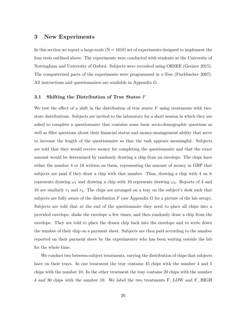
To test the influence of the observability of the true state (test (iii)), we implement the

random draw on the computer and are thus able to recover the true state. We use a double-

blind procedure to alleviate subjects’ concerns about indirect material consequences of lying,

e.g., being excluded from future experiments. We find significantly less over-reporting in the

4

treatment in which the true state is observable compared to when it is not. This finding is

again inconsistent with direct lying cost models and social comparison models since in those

models utility does not depend on the observability of the true state. Moreover, we find that

no subject lies downwards in this treatment (test (iv)).

In Section 4, we compare the predictions of the models to the gathered empirical evidence.

The main empirical finding is that our four tests rule out almost all of the models previously

suggested in the literature. From the set of models we consider, only combining a preference

for being honest with a preference for being seen as honest (or a model whose intuition

and prediction are very similar) can explain the data. This intuition is also present in the

concurrent papers by Khalmetski and Sliwka (2016) and Gneezy et al. (forthcoming). Both

papers assume that individuals suffer from lying cost and want to be perceived as honest.

Also related is the paper by Dufwenberg and Dufwenberg (2017) which assumes that others’

beliefs about the size of the lie matters for utility. We then turn to calibrating a simple, linear

version of our model, showing that it can quantitatively reproduce the data from the meta

study as well as the patterns in our new experiments. In the model, individuals suffer a fixed

cost of lying and a cost that is linear in the probability that they lied (given their report and

the equilibrium report). Both cost components are important.

Section 5 concludes and discusses policy implications. Three key insights follow from our

study. First, our meta analysis shows that the data are not in line with the assumption of

payoff-maximizing reporting but rather with some preference for truth-telling. Second, our

results suggest that these preferences are comprised of two components, a direct cost of lying

that depends on the comparison between the report and the true state, and a reputational

cost for being thought of as a liar. This contrasts with most of the previous literature on

lying aversion which focuses on a single cost component. Finally, policy interventions that

rely on voluntary truth-telling by some participants could be very successful, in particular if

it is made hard to lie while keeping a good reputation.

5

1 Meta Study

1.1 Design

The meta study covers 90 experimental studies containing 429 treatment conditions that

fit our inclusion criteria. We include all studies using the setup introduced by Fischbacher

and Föllmi-Heusi (2013) (which we will refer to as “FFH paradigm”), i.e., in which subjects

conduct a random draw and then report their outcome of the draw, i.e., their state. We require

that the true state is unknown to the experimenter (i.e., we require at least two states) but

that the experimenter knows the distribution of the random draw. We also include studies

in which subjects report whether their prediction of a random draw was correct (as in Jiang

2013). The payoff from reporting has to be independent of the actions of other subjects, but

the reporting action can have an effect on other subjects. The expected payoff level must

not be constant, e.g., no hypothetical studies, and subjects are not allowed to self-select into

the reporting experiment after learning about the rules of the experiment. We only consider

distributions that either (i) have more than two states and are symmetric and single-peaked

(including uniform) or (ii) have two states. This excludes only a handful of treatments in the

literature. For more details on the selection process, see Appendix A.

We contacted the authors of the identified papers and thus obtained the raw data of 54

studies. For the remaining studies, we extract the data from graphs and tables shown in the

papers. This process does not allow to recover additional covariates for individual subjects,

like age or gender, and we cannot trace repeated decisions by the same subject. However,

for most of our analyses, we can reconstruct the relevant raw data entirely in this way. The

resulting data set thus contains data for each individual subject. Overall, we collect data on

270616 decisions by 44390 subjects. Experiments were run in 47 countries which cover 69

percent of world population and 82 percent of world GDP. A good half of the overall sample

are students, the rest consists of representative samples or specific non-student samples like

children, bankers or nuns. Table A.4 lists all included studies. Studies for which we obtained

the full raw data are marked by *.

Having access to the (potentially reconstructed) raw data is a major advantage over more

standard meta studies. We can treat each subject as an independent observation, clustering

over repeated decisions and analyzing the effect of individual-specific co-variates. More im-

6

portantly, we can separately use within-treatment variation (by controlling for treatment fixed

effects), within-study variation (by controlling for study fixed effects) and across-study vari-

ation for identification. For other meta studies using the full individual subject data (albeit

on different topics), see e.g., Harless and Camerer (1994) or Weizsäcker (2010).

Since the potential reports differ widely between studies, e.g., sides of a coin or color of

balls drawn from an urn, we focus on the payoff consequences of a report as its defining char-

acteristic. To make the different studies comparable, we map all reports into a “standardized

report”. Our standardized report has three key properties: (i) if a subject’s report leads to

the lowest possible payoff, the standardized report is −1, (ii) if the report leads to the highest

possible payoff, it is +1 and (iii) if the report leads to the same payoff as the expected payoff

from truthful reporting, the standardized report is 0. In particular we define:

rstandardized = π−E[πtruthful]E[πtruthful]−πmin if π < E[πtruthful]

rstandardized = π−E[πtruthful]πmax−E[πtruthful] if π ≥ E[πtruthful]

where π is the payoff of a given report, πmin the payoff from reporting the lowest possible

state, πmax the payoff from reporting the highest state and E[πtruthful] is the expected payoff

from truthful reporting. For example, a roll of a six-sided die would result in standardized

reports of −1, −0.6, −0.2, +0.2, +0.6, or +1.

In general, without making further assumptions, one cannot say how many people lied or

by how much in the FFH paradigm. We can only say how much money people left on the

table. An average standardized report greater than 0 means that subjects leave less money

on the table than a group of subjects who report fully honestly.

To give readers the possibility to explore the data in more detail, we have made interactive

versions of all meta-study graphs available at www.preferencesfortruthtelling.com. The graphs

allow restricting the data, e.g., only to specific countries. The graphs also provide more

information about the underlying studies and give direct links from the plots to the original

papers.

1.2 Results

Finding 1 The average report is bounded away from the maximal report.

7

Figure 1: Average standardized report by incentive level

Notes: The figure plots standardized report against maximal payoff from misreporting. Standardizedreport is on the y-axis. A value of 0 means that subjects realize as much payoff as a group of subjectswho all tell the truth. A value of 1 means that subjects all report the state that yields the highestpayoff. The maximal payoff from misreporting (converted by PPP to 2015 USD), i.e., the differencebetween the highest and lowest possible payoff from reporting, is on the x-axis (log scale). Each bubblerepresents the average standardized report of one treatment and the size of a bubble is proportionalto the number of subjects in that treatment. “FFH BASELINE” marks the result of the baselinetreatment of Fischbacher and Föllmi-Heusi (2013). The line is the fitted regression line of a quadraticregression (with linear x-axis).

Figure 1 depicts an overview of the data. Standardized report is on the y-axis and the

maximal payoff from misreporting, i.e., πmax − πmin, is on the x-axis (converted by PPP

to 2015 USD). As payoff, we take the expected payoff, i.e., the nominal payoff used in the

experiment times the probability that a subject receives the payoff, in case not all subjects

are paid. Each bubble represents the average standardized report of one treatment. The

size of the bubble is proportional to the number of subjects in that treatment. The baseline

treatment of Fischbacher and Föllmi-Heusi (2013) is marked in the figure. It replicates quite

well.

If all subjects were monetary-payoff maximizers and had no concerns about lying, all

bubbles would be at +1. In contrast, we find that the average standardized report is only

0.234 (95% confidence interval: [0.227, 0.242]; t-test that average is equal to 1: p <0.001).

8

This means that subjects forego about three-quarters of the potential gains from lying. This

is a very strong departure from the standard economic prediction.

This finding turns out to be quite robust. Subjects continue to refrain from lying maxi-

mally when stakes are increased. Figure 1 shows that an increase in incentives affects behavior

only very little. In our sample, the potential payoff from misreporting ranges from cents to 50

USD, a 500-fold increase. The fitted regression line in the figure is from a quadratic regression

(the x-axis is on a log scale) and is slightly hump-shaped. In a linear regression of standard-

ized report on the potential payoff from misreporting, we find that a one dollar increase in

incentives changes the standardized report by -0.005 (using between-study variation as in

Figure 1) or 0.003 (using within-study variation). See Appendix A for more details and for

a comparison of our different identification strategies. This means that increasing incentives

even further is unlikely to yield the standard economic prediction of +1. In Appendix A,

we also show that subjects still refrain from lying maximally when they report repeatedly.

Learning and experience thus do not diminish the effect. Reporting behavior is also quite

stable across countries and adding country fixed effects to our main regression (see Table A.2)

increases the adjusted R2 only from 0.368 to 0.455.

We next analyze the distribution of reports within each treatment.

Finding 2 In each treatment, more than one state is reported with positive probability.

Figure 2 shows the distribution of reports for all experiments using uniform distributions with

six or two states, e.g., six-sided die rolls or coin flips. We exclude the few studies that have

non-linear payoff increases from report to report. The figure covers 68 percent of all subjects

in the meta study (the vast majority of the remaining subjects are in treatments with non-

uniform distributions – where Finding 2 also holds). Each line corresponds to one treatment

and the size of the bubbles is proportional to the number of subjects in that treatment.

The dashed line indicates the truthful distribution. The bold line is the average across all

treatments, the grey area around it the 95% confidence interval of the average. As one can

see, all possible reports are made with positive probability in almost all treatments and the

likelihood of the modal report is far away from 1 in all treatments (all p <0.001).

Finding 3 When the distribution of true states is uniform, the probability of reporting a given

state is increasing in its payoff.

9

The figure also shows that reports that lead to higher payoffs are generally made more often,

both for six-state and two-state distributions. The right panel of Figure 2 plots the likelihood

of reporting the low-payoff state (standardized report of −1) for two-state experiments. The

vast majority of the bubbles are below 0.5 which implies that the high-payoff report is above

0.5. This positive correlation between the payoff of a given state and its likelihood of being

reported holds for all uniform distributions we have data on (OLS regressions, all p<0.001).

Finding 4 When the distribution of true states has more than 3 states, some non-maximal-

payoff states are reported more often than their true likelihood.

Interestingly, some reports that do not yield the maximal payoff are reported more often than

their truthful probability, in particular the second highest report in six-state experiments is

more likely than 1/6 in almost all treatments. Such over-reporting of non-maximal states

occurs in all distributions with more than three states we have data on (see Figure A.7 for

the uniform distributions). We test all non-maximal states that are over-reported against

their truthful likelihood using a binomial test. The lowest p-value is smaller than 0.001 for all

distributions (we exclude distributions for which we have very little data, in particular, only

one treatment).

We relegate additional results and all regression analyses to Appendix A.

10

Figure 2: Distribution of reports (uniform distributions with six and two outcomes)

Notes: The figure depicts the distribution of reports by treatment. The left panel shows treatmentsthat use a uniform distribution with six states and linear payoff increases. The right panel showstreatments that use a uniform distribution with two states. The right panel only depicts the likelihoodthat the low-payoff state is reported. The likelihood of the high-payoff state is 1 minus the depictedlikelihood. The size of a bubble is proportional to the total number of subjects in that treatment.Only treatments with at least 10 observations are included. The dashed line indicates the truthfuldistribution at 1/6 and 1/2. The bold line is the average across all treatments, the grey area aroundit the 95% confidence interval of the average.

2 Theory

The meta study shows that subjects display strong aversion to lying and that this results in

specific patterns of behavior as summarized by our four findings. In this section, we use a

unified theoretical framework to formalize various ways that could potentially explain these

patterns (introduced in Section 2.1). In order to address the breadth of plausible explanations

and to be able to draw robust conclusions, we consider a large number of potential mechanisms,

most of them already discussed, albeit often informally, in the literature. Indeed, one key

contribution of our paper is to formalize in a parallel way a variety of suggested explanations.

There are three broad types of explanations of why subjects seem to be reluctant to lie:

subjects face a lying cost when deviating from the truth; they care about some kind of

11

reputation that is linked to their report (e.g., they care about the beliefs of some audience

that observes their report); or they care about social comparisons or social norms which affect

the reporting decision. In Section 2.2, we discuss one example model for each of the three

types of explanations, including one of the two models that our empirical exercise will not be

able to falsify. We discuss the remaining models in the appendices.

To test the models against each other, we first check whether they are able to explain the

stylized findings of the meta study (Section 2.3). We find that many different models can do

so. We therefore use our theoretical framework to develop four new tests that can distinguish

between the models consistent with the meta study (Section 2.4). Table 1 lists all models and

their predictions. For comparison purposes, we also state the results of our experiments in

the row labeled Data.

2.1 Theoretical Framework

An individual observes state ω ∈ Ωn, drawn i.i.d. across individuals from distribution F (with

pdf f). We will suppose, except where noted, that the drawn state is observed privately by

the individual. We suppose Ωn is a subset of equally spaced natural numbers from ω1 to ωn,

ordered ω1, ω2, . . . , ωn with n > 1. As in the meta study, we only consider distributions F

that have f(ω) ∈ (0, 1) for all ω ∈ Ωn and that either (i) have more than two states and are

symmetric and single-peaked or (ii) have two states. Call this set of distributions F .5 After

observing a state, individuals publicly give a report r ∈ Rn, where Rn is a subset of equally

spaced natural numbers from r1 to rn, ordered r1, r2, . . . , rn. Individuals receive a monetary

payment which is equal to their report r. We suppose that there is a natural correspondence

between each element of Rn and the corresponding element of Ωn. For example, imagine an

individual privately flipping a coin. If they report heads, they receive £10, if they report tails

they receive nothing. Then ω1 = r1 = 0, and ω2 = r2 = 10. We denote the distribution over

reports as G (with pdf g). An individual is a liar if they report r 6= ω. The proportion of liars

at r is Λ(r).

We denote a utility function as φ. For clarity of exposition, we suppose that φ is differen-

tiable in all its arguments, except where specifically noted, although our predictions are true5A handful of papers in the meta study use non-equally spaced states. All our results also hold for these

distributions and for any distribution where the payoffs are not “too” unequally spaced.

12

even when we drop differentiability and replace our current assumptions with the appropriate

analogues (we do maintain continuity of φ). We will also suppose, except where specifically

noted, that sub-functionals of φ are continuous in their arguments.

We suppose that individuals are heterogeneous. They have a type ~θ ∈ Θ, where ~θ is a

vector with J entries, and Θ is the set of potential types ×J [0, κj ], with κj > 0. Each of the

J elements of ~θ gives the relative trade-off experienced by an individual between monetary

benefits and specific non-monetary, psychological costs (e.g., the cost of lying, or reputational

costs). When we introduce specific models, we will only focus on the subvector of ~θ that is

relevant for each model (which will usually contain only one or two entries). We suppose that~θ is drawn i.i.d. from H, a non-atomic distribution on Θ. Each entry θj is thus distributed

on [0, κj ].6 In Appendix D, we show that the set of non-falsified models does not change if we

assume that H is degenerate. The exogenous elements of the models are thus the distribution

F over states and the distribution H over types while the distribution G over reports and

thus the share of liars at r, Λ(r), arise endogenously in equilibrium.

We assume that individuals only report once and there are no repeated interactions. We

suppose a continuum of “subject” players and a single “audience” player (the continuum of

subjects ensures that any given subject has a negligible impact on the aggregate reporting

distribution). The subjects are individuals exactly as described above. The audience takes

no action, but rather serves as a player who may hold beliefs about any of the subjects after

observing the subjects’ reports. The audience could be the experimenter, or another person

the subject reveals their report to, or a subject’s future self (an internal audience). Subjects

do not observe each others’ reports. Utility may depend on others’ actions, strategies, or

beliefs. Because subjects take a single action we can consider a strategy as mapping type and

state combinations (~θ × ω) into a distribution over reports r.7 When an individual’s utility6Our assumptions on κj and H imply that our framework for more general models does not nest, strictly

speaking, the standard model, where individuals only care about their monetary payoff. Instead, the standardmodel is a limit case of our models (where the κs go to 0, or the support of H becomes concentrated on 0).This allows the predictions generated by more general models to be sharply distinguished from the predictionsof the standard model (as opposed to nesting them). The same reasoning applies to other “nested” models,e.g. the lying cost model is a limit case of the lying cost plus reputation model.

7Almost all individuals will play a pure strategy in our framework. This is because all types have measurezero and, given our assumptions on the interaction between ~θ and the costs of lying in the models we consider(detailed below), if an individual of type θ is indifferent between the two reports, then no other type can beindifferent. Because subjects in the experiment are anonymous to each other we also only focus on equilibriawhere strategies cannot depend on the identity of the player (but of course, it can depend on their preferenceparameters).

13

depends on the beliefs or strategies of other players, we consider the Sequential Equilibria of

the induced psychological game, as introduced by Battigalli and Dufwenberg (2009). (The

original psychological game theory framework of Geanakoplos et al. (1989) cannot allow for

utility to depend on others’ strategies, nor updated beliefs.) When utility does not depend

on others’ beliefs or strategies, the analysis can be simplified and we assume the solution

concept to be the set of standard Bayes’ Nash Equilibrium of the game. In some of our

models, an individual’s utility depends only on their own state and report. In this case, our

solution concept is simply individual optimization, but for consistency, we also use the word

equilibrium and strategy to describe the outcomes of these models.

2.2 Primary Models

In this section, we introduce one example for each of the three main categories of lying aver-

sion: lying costs (Section 2.2.1), social norms/comparisons (2.2.2), and reputational concerns

(2.2.3). The remaining models are described in Appendix B. Some of these models represent

other ways of formalizing the effect of descriptive norms and social comparisons on reporting,

including a model of inequality aversion (Appendix B.1); a model that combines lying costs

with inequality aversion (B.2); and a social comparisons model in which only subjects who

could have lied upwards matter for conformity (B.3). Other models build on the idea of rep-

utational concerns and include a model where individuals want to signal to the audience that

they place low value on money (B.4); a model where individuals want to cultivate a reputation

as a person who has high lying costs (B.5); and a model of guilt aversion (B.6). Finally, we

include a model of money maximizing with errors (B.7), and a model that combines lying

costs with expectations-based reference-dependence (B.8). In addition, Appendix C describes

several models that fail to explain the findings of the meta study and that are therefore not

further considered in the body of the paper.

2.2.1 Lying Costs (LC)

A common explanation for the reluctance to lie is that deviating from telling the truth is

intrinsically costly to individuals. The fact that individuals’ utility also depends on the

realized state, not just their monetary payoff, could come from moral or religious reasons;

14

from self-image concerns (if the individual remembers ω and r)8; or from injunctive social

norms of honesty. Such “lying cost” (LC) models have wide popularity in applications and

represent a simple extension of the standard model in which individuals only care about their

monetary payoff. Our formulation of this class of models nests all of the lying cost models

discussed in the literature, including a fixed cost of lying, a lying cost that is a convex function

of the difference between the state and the report, and generalizations that include different

lying cost functions.9

Formally, we suppose individuals have a utility function

φ(r, c(r, ω); θLC)

c is a function that maps to the (weak) positive reals and denotes the cost of lying. We

suppose that c has a minimum when r = ω which is not necessarily unique. (For some

specifications, for example fixed costs of lying, c will not be differentiable in its arguments.)

For our calibrational exercises we normalize c(ω, ω) = 0, so that individuals experience no

cost when they tell the truth. The only element of ~θ that affects utility is the scalar θLC which

governs the weight that an individual applies to the lying cost. We make a few assumptions on

φ. First, φ is strictly increasing in the first argument (r), fixing all the other arguments; this

captures the property that utility is increasing in the monetary payment received. Second, φ

is decreasing in the second argument, fixing all the other arguments, capturing the property

that utility falls as the cost of lying increases. In particular, it is strictly decreasing for all

θLC > 0. Third and fourth, fixing all other arguments, φ is decreasing in θLC , and the cross

partial of φ with respect to c and θLC is strictly negative. This captures the properties that

an individual with a higher draw of θLC has both a higher utility cost of lying, for the same

“sized” lie, and faces a higher marginal cost of lying. In other words utility exhibits increasing

differences with respect to c and θLC .10

8If the individual forgets about their own state ω and cares about what their own future selves think aboutthem, judging only from their report r (similar to Bénabou and Tirole 2006), then our Reputation for Honestymodel, described in Appendix C, may be more appropriate. Only the predictions regarding observability wouldneed to be adjusted if the audience is “internal”. In our setting, given the short length of time between drawof state and report, it seems, however, unlikely that individuals would forget the state but not the report.

9This includes, for example, Ellingsen and Johannesson (2004); Kartik (2009); Fischbacher and Föllmi-Heusi(2013); Gibson et al. (2013); Gneezy et al. (2013); Conrads et al. (2013); Conrads et al. (2014); DellaVignaet al. (2014); and Boegli et al. (2016).

10Our results regarding the LC model can be easily generalized further: they do not require that utility is

15

2.2.2 Social Norms: Conformity in Lying Costs (CLC)

Another potential explanation for lying aversion extends the intuition of the LC model. It

posits that individuals care about social norms or social comparisons which inform their

reporting decision. The leading example is that individuals may feel less bad about lying

if they believe that others are lying, too. Importantly, the norms here are “descriptive” in

the sense that they depend on the behavior of others, rather than injunctive, where they do

not depend on what others are doing (injunctive norms are better captured by LC models).

We call such a model conformity in lying costs (CLC). Such concerns for social norms are

discussed, for example, in Gibson et al. (2013), Rauhut (2013) and Diekmann et al. (2015).

Our model follows the intuition of Weibull and Villa (2005). We suppose that an individual’s

total utility loss from misreporting depends both on an LC cost (as described in the previous

model), but also on the average LC cost in society. Since the latter depends on others’

strategies, we must use the framework that Battigalli and Dufwenberg (2009) developed for

psychological games.

Formally, in the CLC model individuals have a utility function

φ(r, η(c(r, ω), c); θCLC)

c(r, ω) has the same interpretation and assumptions as in the LC model and types are het-

erogeneous in the scalar θCLC (the rest of the vector ~θ again does not affect utility). c is the

average incurred cost of lying in society. This average lying cost is determined in equilibrium,

and thus all individuals know what it is; for notational ease we supress the dependence of c

on the other parameters of the model. η captures the “normalized cost of lying”, i.e. the cost

of lying conditional on the incurred lying costs of everyone else (for our calibrational exercises

we suppose η(0, c) = 0) and is strictly increasing in its first argument. For c > 0, η is strictly

falling in the second argument so that the normalized cost is increasing in the individual’s

own personal lying cost and falling in the aggregate lying cost, i.e., their lying costs are falling

as others lie more (for c = 0, the partial of η with respect to its second argument is 0). As in

decreasing in θLC , only that the restriction on the cross partials hold. We make this restriction as it allows fora natural interpretation of θLC . They also do not depend on individuals all having the same functional form cso long as the assumptions regarding θLC hold. So, for example, our results hold when some individuals havefixed and others convex costs of lying.

16

the previous models φ is strictly increasing in its first argument, and decreasing in the second

argument (strictly so for all θCLC > 0). φ is decreasing in θCLC fixing the first two arguments,

and the cross partial of φ with respect to η and θCLC is strictly negative. These assumptions

are analogous to the ones presented in the previous models and capture the same intuitions.

2.2.3 Reputation for Honesty plus Lying Costs (RH+LC)

A different way to extend the LC model is to allow individuals to experience both an intrinsic

cost of lying, as well as reputational costs associated with inference about their honesty (e.g.,

Khalmetski and Sliwka 2016, Gneezy et al. forthcoming). We suppose that an individual’s

utility is falling in the belief of the audience player that the individual’s report is not hon-

est, i.e., has a state not equal to the report. Akerlof (1983) provides the first discussion in

the economics literature that honesty may be generated by reputational concerns and many

recent papers have built on this intuition.11 Thus, an individual’s utility is belief-dependent,

specifically depending on the audience player’s updated beliefs. Thus, we must use the tools

of psychological game theory to analyze the game. We use the framework of Battigalli and

Dufwenberg (2009) in our analysis.12 Of course, the audience cannot directly observe whether

a player is lying, and has to base their beliefs on the observable report r. Because the audi-

ence player makes correct Bayesian inference based on observing the report and knowing the

equilibrium strategies, their posterior belief about whether an individual is a liar, conditional

on a report r, is Λ(r), the fraction of liars at r in equilibrium. We therefore directly assume

that utility depends on υ(Λ(r)), with v a strictly increasing function.

Since lying costs are our preferred way to capture self-image concerns about honesty, one

possible interpretation of this model is that individuals care about self-image and social image

(i.e., the audience’s beliefs). We focus on a situation where there is additive separability

between the different components of the utility function. Formally, in the RH+LC model11This includes, for example, Mazar et al. (2008); Suri et al. (2011); Hao and Houser (2013); Shalvi and

Leiser (2013); Utikal and Fischbacher (2013); Fischbacher and Föllmi-Heusi (2013); Gill et al. (2013) and Hilbigand Hessler (2013).

12Some researchers have suggested that a simple model in which individuals care only about the audience’sbelief that they are a liar, conditional on their report, could explain behavior. We discuss in Appendix Cwhy such a model fails to match the findings of the meta study, and why reputational concerns need to becombined with some other motive to explain the data within our theoretical framework. See Dufwenberg andDufwenberg (2017) for a model where individuals care about the size of the inferred lie and that can explainthe meta study under different distributional assumptions. Appendix D discusses the role of distributionalassumptions for our results.

17

utility is

φ(r, c(r, ω),Λ(r); θLC , θRH) = u(r)− θLCc(r, ω)− θRHυ(Λ(r))

u is strictly increasing in r. Types are heterogeneous in the scalars θLC and θRH and the

rest of ~θ does not affect utility. c is as described in the LC-model. υ is a strictly increasing

function of Λ(r) with a minimum at 0 (and in calibrational exercises we normalize υ(0) = 0).

Thus the individual likes more money, but dislikes lying and being perceived as a liar by the

audience. In the working paper version of this paper (Abeler et al. 2016) we also consider a

more general function that allows for non-separability.13

2.3 Distinguishing Models Using the Meta Study

We now turn to understanding how our models can be distinguished in the data. The first

test is whether the models can match the four findings of the meta study. We find that all

models listed in Table 1 can do so.

Proposition 1 There exists a parameterization of the LC model, the CLC model, the RH+LC

model and of all other models listed in Table 1 which can explain Findings 1–4 for any number

of states n and for any distribution in F .

All proofs for the paper are collected in Appendix E. The proof for the LC model con-

structs one example utility function, combining a fixed cost and a convex cost of lying, and

then shows that it yields Findings 1–4 for any n and any F ∈ F . Many of the other models

considered in this paper contain the LC model as limit case and can therefore explain Findings

1–4. However, there are several models, e.g., the inequality aversion model (Appendix B.1)

or the Reputation for Being Not Greedy model (B.4) which rely on very different mechanisms

and can still explain Findings 1–4.

2.4 Distinguishing Models Using New Empirical Tests

Proposition 1 shows that the existing literature, reflected in the meta study, cannot pin down

the mechanism which generates lying aversion. The meta study does falsify quite a few popular13If we suppose that H may be atomic, then we can also capture “mixture” models, where each individual

either only cares about lying costs, or only cares about reputational costs, but there is a mix in the totalpopulation. In this case, H would have zero support everywhere where both θs are strictly greater than 0.

18

Table1:

Summaryof

Testab

lePr

edictio

nsMod

elNew

Tests

Section

Can

Exp

lain

MetaStud

ySh

iftin

True

DistributionF

Shift

inBelief

Abo

utRep

ortsG

Observability

ofTrueStateω

LyingDow

nUno

bs./Obs.

LyingCosts

(LC)

Yes

f-in

varia

nce

g-in

varia

nce

o-invaria

nce

No/No

2.2.1

Social

Norms/Com

parisons

Con

form

ityin

LyingCosts

(CLC

)*Ye

sdraw

ingou

taffi

nity

o-invaria

nce

No/No

2.2.2

Inequa

lityAv

ersio

n*Ye

sf-in

varia

nce

affinity

o-invaria

nce

-/-

B.1

Inequa

lityAv

ersio

n+

LC*

Yes

draw

ingin

affinity

o-invaria

nce

-/-

B.2

Cen

soredCLC

*Ye

sf-in

varia

nce

affinity

o-invaria

nce

No/No

B.3

Rep

utation

Rep

utationforHon

esty

+LC

*Ye

sdraw

ingin

-o-shift

-/No

2.2.3

Rep

utationforBe

ingNot

Greed

y*Ye

sf-in

varia

nce

-o-invaria

nce

Yes/Ye

sB.4

LC-R

eputation*

Yes

--

o-shift

-/-

B.5

GuiltAv

ersio

n*Ye

sf-in

varia

nce

affinity

o-invaria

nce

-/-

B.6

Cho

iceEr

ror

Yes

f-in

varia

nce

g-in

varia

nce

o-invaria

nce

Yes/Ye

sB.7

Kőszegi-R

abin

+LC

Yes

-g-in

varia

nce

o-invaria

nce

No/No

B.8

Data

draw

ingin

g-invariance

o-shift

?/No

Notes:The

details

ofthepred

ictio

nsareexplaine

din

thetext.“-”means

that

nospecificpred

ictio

ncanbe

mad

e.The

pred

ictio

nsforshiftsinF

and

Garefortw

o-statedistrib

utions,i.e.,n

=2.

Mod

elswhich

dono

tne

cessarily

have

unique

equilib

riaaremarkedwith

anasteris

k(*).

Forthesemod

els,

thepred

ictio

nsoff-in

varia

ncean

do-invaria

ncemeanthat

thesetof

possible

equilib

riais

invaria

ntto

chan

gesinF

orob

servab

ility.The

pred

ictio

nsof

draw

ingin/out

areba

sedon

theassumptionof

aun

ique

equilib

rium.

19

models, which we discuss in Appendix C, but the data is not strong enough to narrow the set

of surviving models further down. This motivates us to devise four additional empirical tests

which can distinguish between the models that are in line with the meta study. Three of the

four new tests are “comparative statics” and one is an equilibrium property: (i) how does the

distribution of true states affect the distribution of reports; (ii) how does the belief about the

reports of other subjects influence the distribution of reports; (iii) does the observability of

the true state affect the distribution of reports; (iv) will some subjects lie downwards if the

true state is observable. As a prediction (iv’), we also derive whether some subjects will lie

downwards if the true state is not observable, as in the standard FFH paradigm. We cannot

test this last prediction in our data but state it nonetheless as it is helpful in building intuition

regarding the models as well as important for potential applications.14

We derive predictions for each model and for each test using very general specifications

of individual heterogeneity and the functional form. We present predictions for an arbitrary

number of states n and for the special case of n = 2. On the one hand, allowing for an

arbitrary number of states generates predictions that are applicable to a larger set of potential

settings. On the other hand, restricting n = 2 allows us to make sharper predictions, and

thus potentially falsify a larger set of models. For example, for models where individuals care

about what others do (e.g., social comparison models), it doesn’t matter whether individuals

care about the average report or the distribution of reports when n = 2. For models that rule

out downward lying, the binary setting also allows us to back out the full reporting strategy

of individuals without actually observing the true state: the high-payoff state will be reported

truthfully, so we can deduct the expected number of high-payoff states from the high-payoff

reports and we are left with the reports made by the subjects who have drawn the low-payoff

state. Moreover, conducting our new tests with two-state distributions is simpler and easier

to understand for subjects.

The models, as well as the predictions they generate in each of the tests, are listed in Table

1. Since our new experiments testing the effect of shifts in the distributions of true states,

F , and beliefs about others’ reports, G, use two-state distributions (see below for details), we

report the two-state predictions in those columns. Some of the models we consider do not14Peer et al. (2014) and Gneezy et al. (2013) study downward lying in a setting in which at least some

subjects will feel unobserved.

20

guarantee a unique reporting distribution G without additional parametric restrictions. We

discuss in more detail how we deal with potential non-uniqueness for each prediction and we

mark the models which do not necessarily have unique equilibria with an asterisk (*) in Table

1. Importantly, no model is ruled out solely on the basis of predictions that are based on an

assumption of uniqueness. Similarly, the models that cannot be falsified by our data are not

consistent solely because of potential multiplicity in equilibria.

We now turn to discussing our four empirical tests. The first test is about how the

distribution of reports G changes when the higher states are more likely to be drawn (but

while maintaining the same set of support for the distribution). Specifically we suppose that

we induce a shift in F that satisfies first order stochastic dominance. We then look at the

ratio of the reports of the lowest state to the draws of the lowest state: f(ω1)−g(r1)f(ω1) = 1− g(r1)

f(ω1)

. For those models in which no individual lies downwards we can interpret the statistic as the

proportion of people who draw ω1 but report something higher, i.e., r > r1.

Definition 1 A model exhibits drawing in/drawing out/f -invariance if 1 − g′(r1)f ′(ω1) is larger

than/smaller than/the same as 1 − g(r1)f(ω1) for all F , F ′ ∈ F where F ′ strictly first order

stochastically dominates F and they have the same support.

As we will show below, several very different motivations can lead to drawing in. For

example, increasing the true probability of high states increases the likelihood that a high

report is true, leading subjects who care about being perceived as honest, as in our RH+LC

model (Section 2.2.3) to make such reports more often. But increasing the true probability

of high states also increases the likelihood that other subjects report high, pushing subjects

who dislike inequality (Appendix B.2) to report high states. And subjects who compare their

outcome to their recent expectations (Appendix B.8) could also react in this way.15

The second test looks at how an individual’s probability of reporting the highest state will

change when we exogenously shift their belief G about the distribution of reports. We focus

on situations where there is full support on all reports in both beliefs and actuality.15In models where the equilibrium is potentially not unique, caution is needed in interpreting the effect

of changes in F on behavior. We have two types of predictions. First, for some models the set of possibleequilibria is invariant to changes in F . In this case we believe that it is reasonable to assume that our treatmentdoes not induce equilibrium switching and therefore behavior does not change with F . In Table 1 we list thesemodels as exhibiting f -invariance. Second, for other models the set of equilibria changes with changes in F .For these models the predictions of drawing in/out listed in Table 1 are based on the assumption of a uniqueequilibrium.

21

Definition 2 A model exhibits affinity/aversion/g-invariance if g′(rn) is larger than/smaller

than/the same as g(rn) for all F , G′ and G where all exhibit full support and G′ strictly first

order stochastically dominates G and they have the same support.

Such an exercise allows us to test the models in one of three ways. First, in some models,

e.g., inequality aversion (Appendix B.1), individuals care directly about the reports made by

others and thus G (or a sufficient statistic for it) directly enters the utility. Therefore, we

can immediately assess the effect of a shift in G on behavior.16 For these models, shifting

an individual’s belief about G directly alters their best response (and since subjects are best

responding to their G, which may be different from the actual G, we may observe out-of-

equilibrium behavior). These models all feature multiple equilibria, and moreover, they all

predict affinity. Second, in some other models (CLC and CCLC), individuals care about

the strategies that others take in the game and the corresponding amount of lying. In these

models no individual lies downwards and so, for binary states, G contains sufficient information

about strategies and the amount of lying. Thus, shifting G directly alters an individual’s best

response. These models again feature multiple equilibria and predict affinity.

Finally, this exercise allows us, albeit indirectly, to understand what happens when beliefs

about H (the distribution of ~θ) change. Directly changing this belief is difficult since this

requires identifying ~θ for each subject and then conveying this insight to all subjects. For

models with a unique equilibrium, because G is an endogenous equilibrium outcome, shifts

in G can, however, only be rationalized by subjects as shifts in some underlying exogenous

parameter — which has to be H, since our experiment fixes all other parameters (e.g., F

and whether states are observable).17 For many of these models, the conditions defining the

unique equilibrium reporting strategy are invariant to shifts in G and H, which means that

our treatment should not have an effect. For another set of models, in particular Reputation

for Being Not Greedy, RH+LC and LC-Reputation, any given H may give rise to multiple

equilibria, so there is no simple mapping from G to beliefs about H and we cannot make any16Not all models can rationalize all Gs for a given F . We do not directly test whether subjects’ predicted

beliefs about distributions are allowed by any given model, given that we only elicit an average prediction ofbeliefs about reports.

17To specify the updating process more precisely, we suppose that individuals have a single probabilitydistribution H which induces G (and G). In a more complete model, individuals would think many differentpossible H distributions to be possible, and hold a prior over these different distributions. Thus, observing adifferent G would induce a shift in the inferred distribution over the different possible Hs. Given reasonableassumptions about the prior distribution over H our results will continue to hold.

22

prediction about how a shift in G should affect G.

Our third test considers whether or not it matters for the distribution of reports that the

audience player can observe the true state. In particular, we will test whether individuals’

reports change if the experimenter can observe not only the report, but also the state for each

individual.

Definition 3 A model exhibits o-shift if G changes when the true state becomes observable

to the audience, and o-invariance if G is not affected by the observability of the state.

In some of the models we consider, the cost associated with lying are internal and therefore

do not depend on whether an audience is able to observe the state or not. In other models,

however, the costs depend on the inference the audience is able to make, and so observability

of the true state affects predictions.18

Our fourth test comes in two parts. Both parts try to understand whether or not there

are individuals who engage in downward lying, i.e., draw ωi and report rj with j < i. The

first is whether downward lying will occur in an equilibrium with observability of the state by

the audience and where G features full support. The second is an analogous test but in the

situation where the state is not observed by the audience. We will only focus on the former

test in our experiments.

Definition 4 A model exhibits downward lying if for all F and G with full support, there

exists some individual who draws ωi but reports rj where j < i. If there is never such an

individual we say the model does not exhibit downward lying.

As we will show below, there can be a number of reasons why individuals may want to

lie downwards. In models where individuals are concerned with reputation, lying downwards

may be beneficial if low reports are associated with a better reputation than high reports. Al-

ternatively, in models of social comparisons, such as the inequality aversion models, downward

lying may arise because individuals aim to conform to others’ reports.

The following proposition summarizes the predictions for the three models described above.18As for f -invariance, whenever a model has potentially multiple equilibria and this set of equilibria is

invariant to observability, we list the model as exhibiting o-invariance because we believe that pure equilibriumswitching is unlikely to occur. In contrast to drawing in/out, we do not need to assume a unique equilibriumfor o-shift predictions as we do not specify in which direction behavior will move.

23

Proposition 2 • Suppose individuals have LC utility. For an arbitrary number of states

n, we have f -invariance, g-invariance, o-invariance and no lying down when the state

is unobserved or observed.

• Suppose individuals have CLC utility. For arbitrary n, we have no prediction with regard

to shifts in F or in G, o-invariance and no lying down when the state is unobserved or

observed. For n = 2, we have drawing out when the equilibrium is unique and we observe

affinity.

• Suppose individuals have RH+LC utility. For arbitrary n, we have no prediction with

regard to shifts in F or in G, o-shift, potentially lying down when the state is unobserved,

and no lying down when the state is observed. For n = 2, we observe drawing in when

the equilibrium is unique.

Before moving on, we provide some intuition for the results. For simplicity, we focus on

two-state/report distributions. In the LC model, individuals never lie downwards, because

they (weakly) pay a lying cost and also receive a lower monetary payoff when doing so. Since

only their own state and their own report matter for utility, conditional on drawing the low

state, for a fixed ~θ, an individual will always make the same report, regardless of F or G.

Thus, we observe both f -invariance and g-invariance. Last, the lying cost is an internal cost

and does not depend on the inference others are making about any given person. Thus,

individuals do not care whether their state is observed.

In the CLC models, individuals will never lie downwards since, as in the LC model, they

would face a lower monetary payoff as well as a weakly higher cost of lying. Morever, with a

unique equilibrium, as f(ω2) increases, more individuals draw the high state and can report

r2 without having to lie. Thus, the average cost of lying falls. This increases the normalized

cost of lying (η) for all individuals. Thus, an individual who draws ω1, and was indifferent

before between r1 and r2 will now strictly prefer r1. This implies drawing out. However, if the

equilibrium is not unique, we cannot make a specific prediction. In the CLC model, because

G enters directly into the utility function and because no one lies downwards, we can tell

how the individual’s best response changes with shifts in expected G, i.e. G (even without

uniqueness). Fixing F , if g(r2) increases, more people draw the low state but say the high

report. This means that more individuals are expected to lie, and so the normalized cost of

24

lying (η) decreases. Thus, individuals who draw the low report will be more likely to say the

high report, i.e., we have affinity. Last, as in the LC model, these costs do not depend on any

inference others are making, and so individuals do not care whether their state is observed.

In the RH+LC model, because individuals have a concern for reputation and also have

lying costs, they may or may not lie down if the state is unobserved. If an individual is

motivated relatively more by reputational concerns, then they will down if the state is un-

observed. In contrast, if lying costs dominate as a motivation, they will not lie down. If the

state is observed, no one lies downwards. Although multiple equilibria may occur, whenever

the equilibrium is unique, the RH+LC model exhibits drawing in. As f(ω2) increases, some

individuals who previously drew ω1 will now draw ω2. Those individuals now face a lower

“LC” cost when giving the high report (which is in fact zero). Fixing the reputational cost,

this implies some of them will now give the high report (instead of the low report). Fixing

the behavior of others, this reduces the fraction of liars giving the high report and thus the

reputational cost of the high report decreases; and similarly, increases the fraction of liars

giving the low report. This reduces the (relative) cost of giving the high report even more.

Therefore, we observe drawing in. Our intuition here relies on partial equilibrium reasoning,

but the formal proof shows how to extend this to full equilibrium reasoning. Since equilibria

are not necessarily unique, we cannot predict the effect of our G treatments.19 Because the

model includes reputational costs, whether or not the audience observes just the report, or

also the state, matters for behavior.

In Appendix F, we provide additional evidence regarding predictions of the Kőszegi-

Rabin+LC model which are not listed in the table. We also test specific f -invariance predic-

tions for the LC model in a 10-state experiment.19Even with a unique equilibrium, we may observe either aversion, affinity or g-invariance since it depends

on how the distribution of H is perceived to have changed when G shifts. If, for example, the change isinterpreted as a shift by individuals who have low reputational costs, and so care mostly about lying costs,then an increase in g(r2) will be interpreted as more individuals who drew ω1 being willing to give the highreport. This decreases the proportion of truth-tellers at the high report, driving aversion. In contrast, supposethe change is interpreted as a shift by individuals who have medium lying costs, but relatively high reputationalcosts. This means that it is interpreted as a shift in the reports of individuals who drew the high state (sinceindividuals who drew the low state and have medium lying costs are unlikely to ever give the high report). Anincrease in g(r2) is then interpreted as individuals who drew ω2 as being more willing to pay the reputationcost of reporting r2. Thus, the fraction of truth-tellers at r2 increases, driving affinity.

25

3 New Experiments

In this section we report a large-scale (N = 1610) set of experiments designed to implement the

four tests outlined above. The experiments were conducted with students at the University of

Nottingham and University of Oxford. Subjects were recruited using ORSEE (Greiner 2015).

The computerized parts of the experiments were programmed in z-Tree (Fischbacher 2007).

All instructions and questionnaires are available in Appendix G.

3.1 Shifting the Distribution of True States F

We test the effect of a shift in the distribution of true states F using treatments with two-

state distributions. Subjects are invited to the laboratory for a short session in which they are

asked to complete a questionnaire that contains some basic socio-demographic questions as

well as filler questions about their financial status and money-management ability that serve

to increase the length of the questionnaire so that the task appears meaningful. Subjects

are told that they would receive money for completing the questionnaire and that the exact

amount would be determined by randomly drawing a chip from an envelope. The chips have

either the number 4 or 10 written on them, representing the amount of money in GBP that

subjects are paid if they draw a chip with that number. Thus, drawing a chip with 4 on it

represents drawing ω1 and drawing a chip with 10 represents drawing ω2. Reports of 4 and

10 are similarly r1 and r2. The chips are arranged on a tray on the subject’s desk such that

subjects are fully aware of the distribution F (see Appendix G for a picture of the lab setup).

Subjects are told that at the end of the questionnaire they need to place all chips into a

provided envelope, shake the envelope a few times, and then randomly draw a chip from the

envelope. They are told to place the drawn chip back into the envelope and to write down

the number of their chip on a payment sheet. Subjects are then paid according to the number

reported on their payment sheet by the experimenter who has been waiting outside the lab

for the whole time.

We conduct two between-subject treatments, varying the distribution of chips that subjects

have on their trays. In one treatment the tray contains 45 chips with the number 4 and 5

chips with the number 10. In the other treatment the tray contains 20 chips with the number

4 and 30 chips with the number 10. We label the two treatments F_LOW and F_HIGH

26

respectively to indicate the different probabilities of drawing the high state (10 percent vs.

60 percent). Note that the distribution used in F_HIGH first-order stochastically dominates

the distribution in F_LOW in line with Definition 1. We select samples sizes such that the

expected number of low states is the same (and equal to 131) in the two treatments. Thus,

we have 146 subjects in F_LOW and 328 subjects in F_HIGH. Most of the sessions were

conducted in Nottingham and some in Oxford between June and December 2015.

3.2 Results

Finding 5 We observe drawing in, i.e., the statistic 1 − g(r1)f(ω1) is significantly higher in

F_HIGH than F_LOW.

Figure 3 shows the values of the statistic 1− g(r1)f(ω1) across the two treatments. In F_LOW

we expect 131 subjects to draw the low £4 payment and we observe 80 subjects actually

reporting 4, i.e. our statistic is equal to 1 − 80131 = 0.39. In F_HIGH we also expect 131

subjects to draw 4, but only 43 subjects report to have done so, so our statistic is equal to

0.67 (this means that 45 percent of subjects in F_LOW and 87 percent in F_HIGH report

10). This difference of almost 30 percentage points is very large and highly significant (p <

0.001, OLS with robust SE; p < 0.001, χ2 test).20

20This result is based on a pooled sample using observations collected both in Nottingham and Oxford. Weobtain similar results if we focus on each sub-sample separately. Using only the Nottingham sub-sample (n =391), we find a treatment difference of about 27 percentage points (p < 0.001, OLS with robust SE; p < 0.001,χ2 test). Using only the Oxford sub-sample (n = 83), we find a treatment difference of about 32 percentagepoints (p = 0.022, OLS with robust SE; p = 0.023, χ2 test).

27

Figure 3: Effect of shifting the distribution of true states

3.3 Shifting Beliefs About the Distribution of Reports G

Our next set of treatments is designed to test predictions concerning the effects of a shift

in subjects’ beliefs about the distribution of reports, i.e., G. There are three other studies

testing the effect of beliefs on reporting (Rauhut 2013, Diekmann et al. 2015 and Gächter and

Schulz 2016a). These studies affect beliefs by showing to subjects the actual past behavior

of participants. Diekmann et al. (2015) and Gächter and Schulz (2016a) find no effect and

Rauhut (2013) finds a positive effect. Rauhut (2013), however, compares subjects who have

initially too high beliefs that are then updated downwards to subjects who have initially too

low beliefs that are updated upwards. The treatment is thus not assigned fully randomly.

We use an alternative and complementary method. Our strategy to shift beliefs is based

on an anchoring procedure (Tversky and Kahneman 1974): we ask subjects to think about

the behavior of hypothetical participants in the F_LOW experiment and we anchor them to

think about participants who reported the high state more or less often. The advantage of

our design is that we do not need to sample selectively from the distribution of actual past

behavior of other subjects. This could be problematic because, if the past behavior is highly

selected but presented as if representative, it could be judged as implicitly deceiving subjects

and could confound results of an experimental study on deception. We are not aware of other

studies that have used anchoring to affect beliefs before.

28

In our setup, subjects are asked to read a brief description of a “potential” experiment

which follows the instructions used in the F_LOW experiment, i.e., 90 percent probability

of the low payment and 10 percent probability of the high payment. Subjects also have

on their desk the tray with chips and envelope that subjects in the F_LOW experiment

had used. Subjects are then asked to “imagine” two “possible outcomes” of the potential

experiment. There are two between-subject treatments, varying the outcomes subjects are

asked to imagine. In treatment G_LOW the outcomes have 20 percent and 30 percent of

hypothetical participants reporting to have drawn a 10, while in treatment G_HIGH these

shares are 70 percent and 80 percent. Subjects are then asked a few questions about these

outcomes.21 Subjects are then told that the experiment has actually been run in the same

laboratory in the previous year and they are asked to estimate the fraction of participants in

the actual experiment who have reported a 10. Subjects are paid £3 if their estimate is correct

(within an error margin of ±3 percentage points). This mechanism is very simple and easier

to explain and understand than proper scoring rules. It elicits in an incentive-compatible

way the mode (or more precisely, the mid-point of the 6-percentage point interval with the

highest likelihood) of a subject’s distribution of estimates. We use subjects’ estimates to check

whether our anchoring manipulation is successful in shifting subjects’ beliefs.22

Finally, after answering a few additional socio-demographic questions, subjects are told

that they will be paid an additional amount of money on top of their earnings from the belief

elicitation. To determine how much money they are paid, subjects are asked to take part in

the F_LOW experiment themselves. The procedure is identical to the description of F_LOW

in the previous section. The experiments were conducted in Nottingham between March and21Subjects are first asked to compute the truthful chance of drawing a 10 in the potential experiment. For

each of the imagined outcomes, they are then asked to estimate how many of the hypothetical participantswho report a 10 have truly drawn a 10 as well as questions about what could motivate someone who has drawna 4 to report either truthfully or untruthfully. Subjects are then asked to rate the satisfaction of someone whoreports either a 4 or a 10 in the potential experiment. Finally subjects are asked to estimate which of the twoimaginary outcomes shown to them they think is “more realistic”. Note that we did not ask subjects to guessor interpret the purpose of the experiment, but rather to reflect on participants’ motives and satisfaction withvarious hypothetical behaviors undertaken in the experiment.

22For many distributions mode and mean are actually tightly linked. To illustrate this point, we have runthe following simulation assuming that beliefs are distributed according to the very flexible beta distribution.We have generated 100000 pairs of beta distributions with randomly drawn α and β and compared the modesand means of the two distributions in each pair. In over 97 percent of cases where a mode exists and whereone distribution has a higher mode than the other one, the higher-mode distribution has also a higher mean.This means that if our elicitation of the belief mode finds a difference between treatments, then it is highlylikely that the two treatments also have different belief means.

29

May 2016 with a total of 340 subjects (173 in G_LOW, 167 in G_HIGH).

3.4 Results

We start by showing the effect of the anchors on subjects’ beliefs.

Finding 6 The anchors significantly shift beliefs. Estimates of the fraction of participants

reporting a 10 are more than 20 percentage points higher in G_HIGH than G_LOW.

Figure 4 shows the distributions of estimates of the proportion of reported 10s made by

subjects across the two treatments. The distribution of the G_HIGH treatment is strongly

shifted to the right relative to G_LOW, and practically first-order stochastically dominates

it, in line with Definition 2. On average, subjects in G_LOW believe that 41 percent of

participants in the F_LOW experiment have reported a 10. In G_HIGH the average belief

is 62 percent (p < 0.001, OLS with robust SE; p < 0.001, Wilcoxon rank-sum test).

Figure 4: Distribution of beliefs about proportion of reported 10s

Having established that our manipulation is successful in shifting beliefs about reports

in the expected direction, our next step is to examine the effects of this shift in beliefs on

subjects’ actual reporting behavior.

Finding 7 The fraction of subjects reporting a 10 is not significantly different between G_HIGH

and G_LOW, i.e., we find g-invariance.

30

Figure 5 shows the share of subjects reporting a 10 across the two treatments. Recall that

in both treatments the true probability of drawing a 10 is 10 percent (this is indicated by the

dashed line in the figure). We observe 55 percent of subjects reporting a 10 in G_LOW, and

49 percent in G_HIGH. This difference is not significant (p = 0.285, OLS with robust SE;

p= 0.311, 2SLS regressing report on belief with treatment as instrument for belief; p = 0.284,

χ2 test). Taken together, our study and the previous literature provide converging evidence

that manipulating beliefs about others’ reports has a limited impact on reporting.

One word of caution is warranted. Even though the point estimate of the effect of the

G treatments is quite close to zero, we cannot reject (small) positive or negative effects of a

change in beliefs. A power analysis shows that we can only detect treatment differences of 15

percentage points or larger at the 5% level and with 80% power, but we are not sufficiently

powered to detect small differences like that observed in Figure 5. This may raise the concern

that our rejection of many models, in particular the social comparisons models, which all

predict affinity, is driven by a lack of power. However, these models typically predict quite

large responses to shifts in G. For example, a simple, calibrated version of the CLC model

implies that 21 percent of subjects should increase their reports across our G treatments,

which we do have power to detect. In fact, our data show that (in net) 6 percent of subjects

decrease their report.23

23The 95 percent confidence interval of the difference between the share of high reports across our G treat-ments is from 0.049 to -0.165. We focus on the CLC model as it provides a baseline utility function formodeling social comparisons and cleanly demonstrates the fact that we should expect to see large shifts in ourG treatments. For details of this calibration see Appendix E.5.

31

Figure 5: Effect of shifting beliefs about the distribution of reports

3.5 Changing the Observability of States

A final set of treatments tests whether observability of the subject’s true state by the exper-

imenter affects reporting behavior, in line with Definition 3. The experiments use a setup

similar to the one described above. Subjects are invited to the lab to fill in a questionnaire

and are paid based on a random draw that they perform privately. There are two between-

subject treatments. Differently from the previous experiments, in both treatments the draw

is performed out of a 10-state uniform distribution. In our UNOBSERVABLE treatment, the

draw is performed using the same procedures described for the previous experiments: subjects

draw a chip at random out of an envelope, report the outcome on a payment sheet, and are

paid based on this report. Thus, in this treatment the experimenter cannot observe the true

state of a subject and cannot tell for any individual subject whether they lie or tell the truth.

In our OBSERVABLE treatment we maintain this key feature of the FFH paradigm, but

make subjects’ true state observable to the experimenter. In order to do so, the procedure

of the OBSERVABLE treatment differs from the UNOBSERVABLE treatment in two ways.

First, the draw is performed using the computer instead of the physical medium of our other

experiments (the chips and the envelope).24 Second, we introduce a payment procedure that24The computerized program simulates the process of drawing a chip from an envelope. Subjects first see on

their screen a computerized envelope containing 50 chips numbered between 1 and 10. Subjects have to clicka button to start the draw. The chips are then shuffled in the envelope for a few seconds and then one chip at

32

makes it impossible for the experimenter to link a report to an individual subject. Before the

start of the experiment the experimenter places an envelope containing 10 coins of £1 each on

each subject’s desk. Subjects are told to sit “wherever they want” and sit down unsupervised.

The experimenter does thus not known which subject is at which desk. After the computerized

draw, instead of writing the number on their chip on the payment sheet, subjects are told to

take as many coins from the envelope as the number of their chip. Subjects then leave the lab

without signing any receipt for the money taken or meeting the experimenter again. At the end

of the experiment, the experimenter counts the number of coins left by subjects on each desk

to reconstruct their “report” and compares it to the true state drawn on the corresponding

computer without being able to link any report to the identity of a subject.25 We ran these

experiments at the University of Nottingham with 288 subjects (155 in UNOBSERVABLE;

133 in OBSERVABLE). Experiments were conducted between May and October 2015.

3.6 Results

Figure 6 shows the distribution of reports in the UNOBSERVABLE and OBSERVABLE

treatments. The dashed line in the figure indicates that in both treatments the truthful

probability of drawing each state is 10 percent.

Finding 8 Introducing observability has a strong and significant effect on the distribution of

reports.

random falls out of the envelope. Subjects are told that the number of that chip corresponds to their paymentamount. For comparability, the computer is also used in the UNOBSERVABLE treatment where subjects useit to get precise information on how to perform the (physical) draw.

25Had we only introduced observability of states without the double-blind payment procedure, we wouldhave deviated from the FFH paradigm whereby an individual cannot be caught lying. This could confoundthe results because additional concerns may have come to the fore in subjects’ mind. For instance, they mayhave become concerned with material punishment for misreporting their draw (e.g. exclusion from futureexperiments). As a robustness check, we invited an additional 69 subjects to participate in a version ofthe OBSERVABLE treatment that did not use the double-blind payment procedure. The share of subjectsmisreporting their draw is lower when we do not use the double-blind payment procedure though this effect isnot significant.

33

Figure 6: Effect of changing the observability of states

Reports in the UNOBSERVABLE treatment are considerably higher than in the OB-

SERVABLE treatment (p < 0.001 OLS with robust SE; p < 0.001 Kolmogorov-Smirnov test;

p < 0.001, Wilcoxon rank-sum test; see Kajackaite and Gneezy (2017) for a similar result).

This result also demonstrates that it would be misleading to rely on evidence from set-

tings in which the true state is observable by the researcher if one is actually interested in

understanding a setting in which the true state is truly unobservable.

We can also use the OBSERVABLE treatment to examine our prediction about the ex-

istence of downward lying when the state is observable (Definition 4). Importantly, we may

not have the same result in a setting where the true state is unobservable (see Table 1).

Finding 9 There is no downward lying when the true state is observable.

Figure 7 shows a scatter plot of subjects’ reports and true draws in the OBSERVABLE

treatment. The size of the bubbles reflects the underlying number of observations. No subject

reported a number lower than their true draw, i.e. lied downwards. About 60 percent of the

subjects who lie report the highest possible number, the remaining 40 percent of liars report

non-maximal numbers.

34

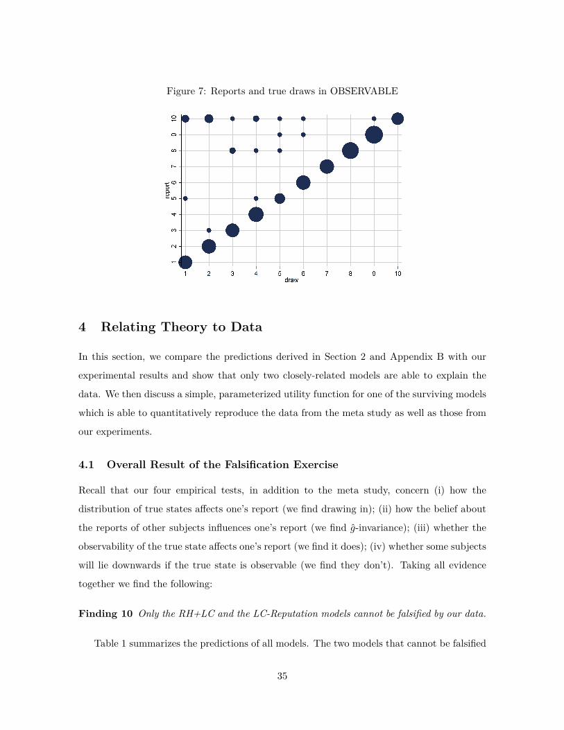
Figure 7: Reports and true draws in OBSERVABLE

4 Relating Theory to Data

In this section, we compare the predictions derived in Section 2 and Appendix B with our

experimental results and show that only two closely-related models are able to explain the

data. We then discuss a simple, parameterized utility function for one of the surviving models

which is able to quantitatively reproduce the data from the meta study as well as those from

our experiments.

4.1 Overall Result of the Falsification Exercise

Recall that our four empirical tests, in addition to the meta study, concern (i) how the

distribution of true states affects one’s report (we find drawing in); (ii) how the belief about

the reports of other subjects influences one’s report (we find g-invariance); (iii) whether the

observability of the true state affects one’s report (we find it does); (iv) whether some subjects

will lie downwards if the true state is observable (we find they don’t). Taking all evidence

together we find the following:

Finding 10 Only the RH+LC and the LC-Reputation models cannot be falsified by our data.

Table 1 summarizes the predictions of all models. The two models that cannot be falsified

35

by our data, RH+LC and LC-Reputation, combine a preference for being honest with a

preference for being seen as honest. In RH+LC, individuals care about lying costs and about

the probability of being a liar given their report. In LC-Reputation, individuals care about

lying costs and about what an audience observing the report deduces about their lying cost

parameter θLC .

All other models fail at least one of the four tests. Looking at Table 1, one can discern

certain patterns. The LC model, which is most widely used in the literature, fails two tests,

predicting f -invariance and o-invariance. The CLC model, which is our preferred way to

model the effect of descriptive norms, fails three tests, predicting drawing out (when the

equilibrium is unique), affinity and o-invariance. All other social comparisons models also

predict affinity and o-invariance. Moreover, as we discuss in Appendix C, several popular

models, like the standard model and models that assume that subjects only care about their

reputation for having been honest, cannot even explain the findings of the meta study (and

also fail our new tests).26

We find no significant effect of a change in beliefs, i.e., g-invariance. As we discussed

in Section 3.4, our study is sufficiently powered to detect treatment differences implied by

reasonably parametrized versions of the social comparison models, e.g., CLC. We cannot,

however, rule out (small) positive or negative effects of a change in beliefs. Regardless of

whether our G treatments have enough power or not, even if we interpreted our data on this

test as inconclusive and thus disregard the g-invariance result, we can still reject all the social

comparisons models because they fail at least one other experimental test.

Importantly, non-uniqueness of equilibria does not affect our overall falsification. Recall

that the first and third test might not work when there is more than one equilibrium. All

those models that fail the first or third test and could feature multiple equilibria also fail

additional tests. Similarly, the models that our data cannot falsify are consistent with the

data when the equilibrium is unique.26Some researchers, such as Crawford et al. (2013) and Wang et al. (2010), have interpreted evidence from

communication games as supportive of level-k reasoning. Our data is consistent with that conclusion. However,our results indicate that level-k reasoning alone is not sufficient to generate the observed behavior. There mustbe some additional factor, such as LC type motivations. Similarly, level-k reasoning is not necessary for amodel to be consistent with our data.

36

4.2 A Calibrated Utility Function

In order to demonstrate how one of the non-falsified models, the RH+LC model (Section

2.2.3), can quantitatively match both the data from the meta study and from our new ex-

periments, we calibrate a simple, linear functional form. Our calibration is not intended to

suggest that the functional form presented here, along with our choice of H, best matches

the data. Instead, we view this as a demonstration that even quite simple and tractable as-

sumptions generate equilibria that allow us to capture many of the important features of the

data. Enriching the model further will only improve the fit. We suggest the following utility

function which we call “Calibrated RH+LC”:

φ(r, c(r, ω),Λ(r); θRH) = r − cIω 6=r − θRHΛ(r)

As before, r is the report, ω the true state and Λ(r) the fraction of liars at r. c is a fixed

cost of lying and Iω 6=r is an indicator function of whether an individual lied. We suppose all

individuals experience the same fixed cost of lying (this utility function is thus a limit case

of the RH+LC model). The individual-specific weight on reputation, θRH , is drawn from a

uniform distribution on [0, κRH ]. The average θRH is thus κRH/2. Additional details of the

calibration are in Appendix E.6.27

We calibrate the model to match the leading example in the literature, a simple die-roll

setting, i.e., a uniform distribution F over six possible states with payoffs ranging from 1 to

6, where the audience cannot observe the state. We set c = 3 and κ = 12. We find that

in the equilibrium, no individual lies down. Moreover, Λ(ri) = 0 for i ≤ 4, Λ(r5) ≈ 0.15

and Λ(r6) ≈ 0.37. We find a reporting distribution similar to that found in our meta study:

g(r1) ≈ 0.07, g(r2) ≈ 0.13, g(r3) ≈ 0.17, g(r4) ≈ 0.17, g(r5) ≈ 0.20 and g(r6) ≈ 0.27. Figure

8 compares the predicted reporting distribution of this calibrated model to the data. The fit

is quite good, in particular given the simple functional form, and the model matches all four

findings of the meta study.

It also matches up with our experimental findings. In a setting where the state is observ-27In concurrent work, Khalmetski and Sliwka (2016) and Gneezy et al. (forthcoming) discuss another limit

case of the RH+LC model, where all individuals face the same reputational cost, but vary in the LC componentof utility. Such utility functions can also be calibrated to match both the meta study data and our newexperiments.

37

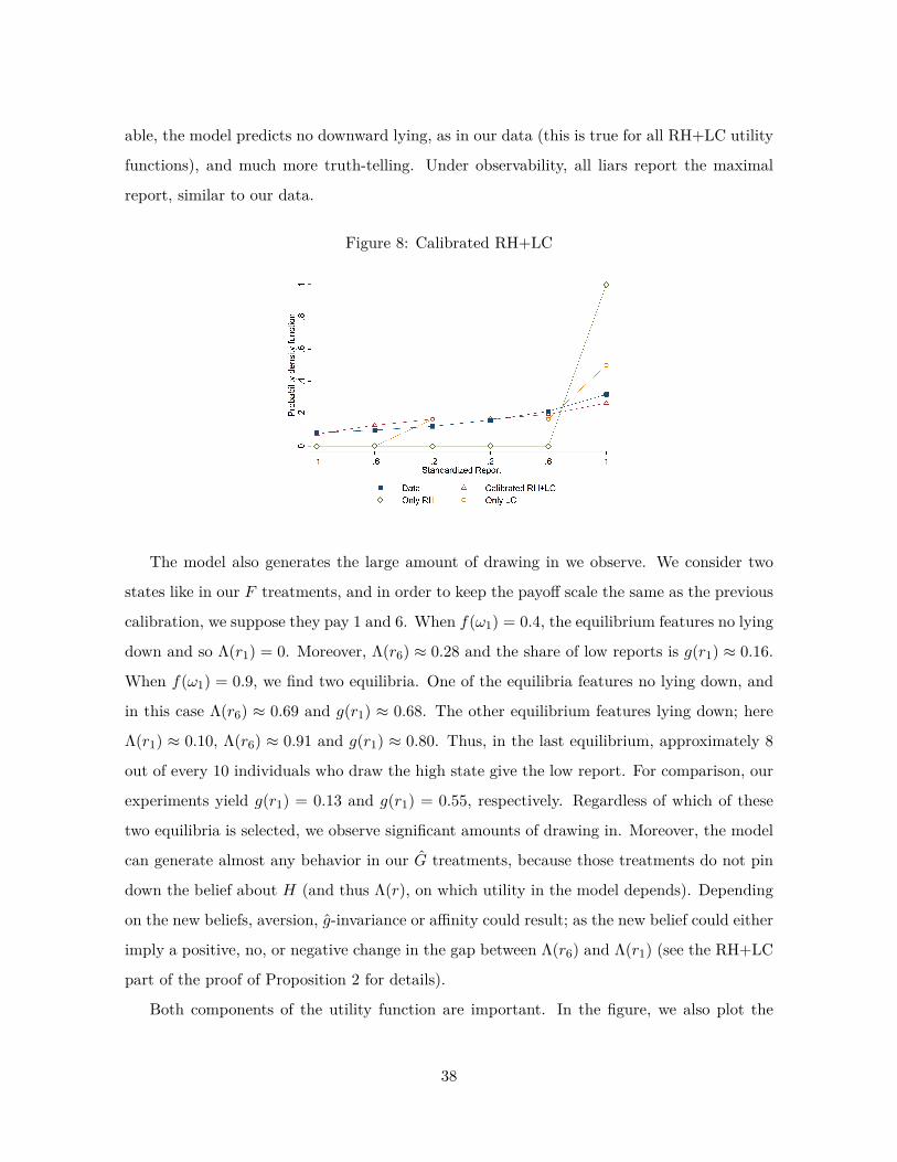
able, the model predicts no downward lying, as in our data (this is true for all RH+LC utility

functions), and much more truth-telling. Under observability, all liars report the maximal

report, similar to our data.

Figure 8: Calibrated RH+LC

The model also generates the large amount of drawing in we observe. We consider two

states like in our F treatments, and in order to keep the payoff scale the same as the previous

calibration, we suppose they pay 1 and 6. When f(ω1) = 0.4, the equilibrium features no lying

down and so Λ(r1) = 0. Moreover, Λ(r6) ≈ 0.28 and the share of low reports is g(r1) ≈ 0.16.

When f(ω1) = 0.9, we find two equilibria. One of the equilibria features no lying down, and

in this case Λ(r6) ≈ 0.69 and g(r1) ≈ 0.68. The other equilibrium features lying down; here

Λ(r1) ≈ 0.10, Λ(r6) ≈ 0.91 and g(r1) ≈ 0.80. Thus, in the last equilibrium, approximately 8

out of every 10 individuals who draw the high state give the low report. For comparison, our

experiments yield g(r1) = 0.13 and g(r1) = 0.55, respectively. Regardless of which of these

two equilibria is selected, we observe significant amounts of drawing in. Moreover, the model

can generate almost any behavior in our G treatments, because those treatments do not pin

down the belief about H (and thus Λ(r), on which utility in the model depends). Depending

on the new beliefs, aversion, g-invariance or affinity could result; as the new belief could either

imply a positive, no, or negative change in the gap between Λ(r6) and Λ(r1) (see the RH+LC

part of the proof of Proposition 2 for details).

Both components of the utility function are important. In the figure, we also plot the

38

predicted reporting distributions for the utility function when we shut down the LC or the

RH part. The Only-RH model is far away from the data. The Only-LC model is closer, but

this model does not generate drawing in or o-shift.28

5 Conclusion

Our paper attempts to understand the constituent mechanisms that drive lying aversion.

Drawing on the extensive experimental literature following the FFH paradigm, we establish

some “stylized” findings within the literature, demonstrating that even in one-shot anonymous

interactions with experimenters, many subjects do not lie maximally. Our new experimental

results, combined with our theoretical predictions, demonstrate that the best description of

why people lie is likely to be a model which incorporates multiple types of costs, which have

usually been thought of in isolation. In particular, we show that among the many models

we consider only a model that combines a desire to be honest with a desire to appear honest

cannot be falsified by our data. While we focus on a situation of individual decision making,

the utility functions we consider should be present in all situations that involve the reporting

of private information, e.g., sender-receiver games, and would there form the basis for the

strategic interaction.29

Three concurrent papers also present models that incorporate a desire to appear honest

in the utility function. Dufwenberg and Dufwenberg (2017) present a more nuanced formal-

ization of the desire to appear honest. In their model, the individual cares about the beliefs

that an audience has about the size of the lie, and not just about whether an individual has

lied. Such a model can explain the results of the original Fischbacher and Föllmi-Heusi (2013)

setup. The utility functions proposed by Khalmetski and Sliwka (2016) and Gneezy et al.

(forthcoming) are similar in spirit to our RH+LC model. Both papers combine a desire to ap-

pear honest with a desire to be honest. Khalmetski and Sliwka (2016) show that a calibrated

version of their model reproduces the data patterns observed in the FFH paradigm. Similar28In the Only-LC model, individuals who draw ω3 are indifferent between reporting r3 and r6. We suppose

for the figure that they say r3. Shifting these to r6 only worsens the fit.29Focusing more narrowly on experiments, our insights also do not just pertain to setups similar to Fis-

chbacher and Föllmi-Heusi (2013). The matrix task of Mazar et al. (2008), described in the introduction, andother real-effort reporting tasks add ambiguity about the true proportion of correct answers in the populationbut once our models are adjusted to take the ambiguity into account, they can be directly applied to the Mazaret al. (2008) setting.

39

to two of our new tests, Gneezy et al. (forthcoming) present experiments that manipulate the

true distribution of the states as well as the observability of the state, with similar results to

our tests. Taken together, the results of these two latter studies reinforce our finding that

multiple types of costs, and in particular a combination of lying costs and reputational costs,

are needed to understand the drivers of lying aversion. Combining Dufwenberg and Dufwen-

berg’s version of reputation with direct lying costs would be an interesting avenue for future

research.

What lessons can we draw for policy? The size and robustness of the effect we document

suggest that mechanisms that rely on voluntary truth-telling by some participants could be

very successful. They could be easier or cheaper to implement and they could achieve outcomes

that are impossible to achieve if incentive compatibility is required. Moreover, if the social

planner wants to increase truth-telling in the population, our preferred model suggests that

lying costs and concerns for reputation are important. Thus, whatever created the lying costs

in the first place, e.g., education or a Hippocratic oath-type professional norm, is effective and

should be strengthened. In addition, one should try to make it harder to lie while keeping a

good reputation, e.g., via transparency, naming-and-shaming or reputation systems.

There are at least four potential caveats for these policy implications. First, we would

not normally base recommendations on a single lab experiment. Given that our meta study

provides very strong, large-scale evidence, however, we feel confident that truth-telling is a

robust phenomenon. Second, lab experiments are not ideal to pin down the precise value of

policy-relevant parameters. We would thus not put much emphasis on the exact value of, say,

the average amount of lying, which we measure as 0.234. However, it is clear that, whatever

the exact value is, it is far away from 1. Thirdly, none of our results suggests that all people in

all circumstances will shy away from lying maximally. Any mechanism that relies on voluntary

truth-telling will need to be robust to some participants acting rationally and robust to self-

selection of rational participants into the mechanism. Finally, the FFH paradigm does not

capture several aspects that could affect reporting. Subjects have to report and they have to

report a single number. This excludes lies by omission or vagueness (Serra-Garcia et al. 2011).

From the viewpoint of the subject, there is also little ambiguity about whether they lied or

not. In reality a narrative for reporting a higher state while still maintaining a self-image of

honesty might be easier to generate (Tirole et al. 2017, Mazar et al. 2008).

40

6 ReferencesJ. Abeler. A reporting experiment with Chinese professionals. mimeo, 2015.J. Abeler and D. Nosenzo. Lying and other preferences. mimeo, 2015.J. Abeler, A. Falk, L. Goette, and D. Huffman. Reference points and effort provision. American

Economic Review, 101(2):470–492, 2011.J. Abeler, A. Becker, and A. Falk. Representative evidence on lying costs. Journal of Public

Economics, 113:96–104, 2014.J. Abeler, D. Nosenzo, and C. Raymond. Preferences for truth-telling. IZA Discussion Paper

No 10188, 2016.G. Akerlof. Loyalty filters. American Economic Review, 73(1):54–63, 1983.M. Allingham and A. Sandmo. Income tax evasion: A theoretical analysis. Journal of Public

Economic, 1:323–338, 1972.A. Amir, T. Kogut, and Y. Bereby-Meyer. Careful cheating: people cheat groups rather than

individuals. Frontiers in Psychology, 7, 2016.J. Andreoni and D. Bernheim. Social image and the 50–50 norm: A theoretical and experi-

mental analysis of audience effects. Econometrica, 77(5):1607–1636, 2009.M. Antony, H. Gerhardt, and A. Falk. The impact of food and water deprivation on economic

decision making. mimeo, 2016.Y. Arbel, R. Bar-El, E. Siniver, and Y. Tobol. Roll a die and tell a lie–what affects honesty?

Journal of Economic Behavior & Organization, 107:153–172, 2014.D. Ariely, X. Garcia-Rada, L. Hornuf, and H. Mann. The (true) legacy of two really existing

economic systems. University of Munich Discussion Paper, 2014.G. Aydogan, A. Jobst, K. D’Ardenne, N. Müller, and M. Kocher. The detrimental effects of

oxytocin-induced conformity on dishonesty in competition. Psychological Science, forth-coming.

R. Banerjee, N. Datta Gupta, and M. C. Villeval. The spillover effects of affirmative actionon competitiveness and unethical behavior. IZA Discussion Paper No 10394, 2016.

S. Barfort, N. Harmon, F. Hjorth, and A. L. Olsen. Dishonesty and selection into publicservice in Denmark: Who runs the world’s least corrupt public service? University ofCopenhagen Discussion Paper, 2015.

Z. Basic, A. Falk, and S. Quercia. The influence of self and social image concerns on lying.mimeo, 2016.

D. Batson, D. Kobrynowicz, J. Dinnerstein, H. Kampf, and A. Wilson. In a very differentvoice: Unmasking moral hypocrisy. Journal of Personality and Social Psychology, 72(6):1335, 1997.

D. Batson, E. Thompson, G. Seuferling, H. Whitney, and J. Strongman. Moral hypocrisy: Ap-pearing moral to oneself without being so. Journal of Personality and Social Psychology,77(3):525, 1999.

P. Battigalli and M. Dufwenberg. Guilt in games. American Economic Review, 97(2):170–176,2007.

P. Battigalli and M. Dufwenberg. Dynamic psychological games. Journal of Economic Theory,

41

144(1):1–35, 2009.T. Beck, C. Bühren, B. Frank, and E. Khachatryan. Lying in the face of monitoring, reci-

procity, and commitment. mimeo, 2016.R. Bénabou and J. Tirole. Incentives and prosocial behavior. American Economic Review, 96

(5):1652–1678, 2006.M. Blanco and J.-C. Cárdenas. Honesty after a labor relationship. Universidad del Rosario

Discussion Paper, (2015-37), 2015.A. Boegli, B. Rockenbach, J. Sobel, and A. Wagner. Why do people tell the truth? A

classifcation approach. mimeo, 2016.G. Bolton and A. Ockenfels. ERC: A theory of equity, reciprocity, and competition. American

Economic Review, 90(1):166–193, 2000.S. Braun and L. Hornuf. Leadership and persistency in spontaneous dishonesty. IAAEU

Discussion Paper, 2015.C. Bryan, G. Adams, and B. Monin. When cheating would make you a cheater: Implicating

the self prevents unethical behavior. Journal of Experimental Psychology: General, 142(4):1001, 2013.

A. Bucciol and M. Piovesan. Luck or cheating? A field experiment on honesty with children.Journal of Economic Psychology, 32(1):73–78, 2011.

B. Cadsby, N. Du, and F. Song. In-group favoritism and moral decision-making. Journal ofEconomic Behavior and Organization, 128:59–71, 2016.

A. W. Cappelen, O.-H. Fjeldstad, D. Mmari, I. H. Sjursen, and B. Tungodden. Managingthe resource curse: A survey experiment on corruption expectations in Tanzania. mimeo,2016.

J. C. Cardenas and J. Carpenter. Behavioural development economics: Lessons from fieldlabs in the developing world. Journal of Development Studies, 44(3):311–338, 2008.

G. Charness and M. Dufwenberg. Promises and partnership. Econometrica, 74(6):1579–1601,2006.

G. Charness, C. Blanco, L. Ezquerra, and I. Rodriguez-Lara. Cheating, incentives, and moneymanipulation. mimeo, 2017.

J. Chytilova and V. Korbel. Individual and group cheating behavior: a field experiment withadolescents. IES Working Paper, 2014.

S. Clot, G. Grolleau, and L. Ibanez. Smug alert! Exploring self-licensing behavior in a cheatinggame. Economics Letters, 123(2):191–194, 2014.

A. Cohn and M. A. Maréchal. Laboratory measure of cheating predicts school misconduct.Economic Journal, forthcoming.

A. Cohn, E. Fehr, and M. A. Maréchal. Business culture and dishonesty in the bankingindustry. Nature, 516(7529):86–89, 2014.

A. Cohn, M. A. Maréchal, and T. Noll. Bad boys: How criminal identity salience affects ruleviolation. Review of Economic Studies, 82(4):1289–1308, 2015.

A. Cohn, T. Gesche, and M. Maréchal. Honest communication in the digital age. mimeo,2016.

D. Cojoc and A. Stoian. Dishonesty and charitable behavior. Experimental Economics, 17

42

(4):717–732, 2014.J. Conrads and S. Lotz. The effect of communication channels on dishonest behavior. Journal

of Behavioral and Experimental Economics, 58:88–93, 2015.J. Conrads, B. Irlenbusch, R. M. Rilke, and G. Walkowitz. Lying and team incentives. Journal

of Economic Psychology, 34:1–7, 2013.J. Conrads, B. Irlenbusch, R. M. Rilke, A. Schielke, and G. Walkowitz. Honesty in tourna-

ments. Economics Letters, 123(1):90–93, 2014.J. Conrads, M. Ellenberger, B. Irlenbusch, E. Ohms, R. Rilke, and G. Walkowitz. Team goal

incentives and individual lying behavior. WHU Discussion Paper, 2017.V. Crawford and J. Sobel. Strategic information transmission. Econometrica, 50(6):1431–

1451, 1982.V. P. Crawford, M. A. Costa-Gomes, and N. Iriberri. Structural models of nonequilibrium

strategic thinking: Theory, evidence, and applications. Journal of Economic Literature,51(1):5–62, 2013.

G. d’Adda, D. Darai, and R. A. Weber. Do leaders affect ethical conduct? CESifo DiscussionPaper, 2014.

Z. Dai, F. Galeotti, and M. C. Villeval. Cheating in the lab predicts fraud in the field. Anexperiment in public transportations. Management Science, forthcoming.

S. Dato and P. Nieken. Compensation and honesty: Gender differences in lying. mimeo, 2015.S. DellaVigna, J. List, U. Malmendier, and G. Rao. Voting to tell others. NBER Discussion

Paper, 2014.S. Demichelis and J. W. Weibull. Language, meaning, and games: A model of communication,

coordination, and evolution. American Economic Review, 98(4):1292–1311, 2008.S. Di Falco, B. Magdalou, D. Masclet, M. C. Villeval, and M. Willinger. Can transparency of

information reduce embezzlement? Experimental evidence from Tanzania. mimeo, 2016.A. Dieckmann, V. Grimm, M. Unfried, V. Utikal, and L. Valmasoni. On trust in honesty

and volunteering among Europeans: Cross-country evidence on perceptions and behavior.European Economic Review, forthcoming.

A. Diekmann, W. Przepiorka, and H. Rauhut. Lifting the veil of ignorance: An experimenton the contagiousness of norm violations. Rationality and Society, 27(3):309–333, 2015.

B. M. Djawadi and R. Fahr. “. . . and they are really lying”: Clean evidence on the perva-siveness of cheating in professional contexts from a field experiment. Journal of EconomicPsychology, 48:48–59, 2015.

M. Drupp, M. Khadjavi, and M. Quaas. Truth-telling to the regulator? Evidence from a fieldexperiment with commercial fishermen. mimeo, 2016.

R. Duch and H. Solaz. Who cheats: Experimental evidence from the lab.M. J. Dufwenberg and M. S. Dufwenberg. Lies in disguise – A theoretical analysis of cheating.

CESifo Discussion Paper 6208, 2017.D. Effron, C. Bryan, and K. Murnighan. Cheating at the end to avoid regret. Journal of

personality and social psychology, 109(3):395, 2015.T. Ellingsen and M. Johannesson. Promises, threats and fairness. The Economic Journal,

114(495):397–420, 2004.

43

T. Ellingsen and M. Johannesson. Pride and prejudice: The human side of incentive theory.American Economic Review, 98(3):990–1008, 2008.

T. Ellingsen and R. Östling. When does communication improve coordination? AmericanEconomic Review, 100(4):1695–1724, 2010.

C. Engel. Dictator games: A meta study. Experimental Economics, 14(4):583–610, 2011.E. Eyster and M. Rabin. Cursed equilibrium. Econometrica, 73(5):1623–1672, 2005.E. Fehr and K. M. Schmidt. A theory of fairness, competition, and cooperation. Quarterly

journal of Economics, 114:817–868, 1999.U. Fischbacher. z-Tree: Zurich toolbox for ready-made economic experiments. Experimental

Economics, 10(2):171–178, 2007.U. Fischbacher and F. Föllmi-Heusi. Lies in disguise—an experimental study on cheating.

Journal of the European Economic Association, 11(3):525–547, 2013.A. Foerster, R. Pfister, C. Schmidts, D. Dignath, and W. Kunde. Honesty saves time (and

justifications). Frontiers in Psychology, 4, 2013.T. R. Fosgaard. Asymmetric default bias in dishonesty–how defaults work but only when in

one’s favor. University of Copenhagen Discussion Paper, 2013.T. R. Fosgaard, L. G. Hansen, and M. Piovesan. Separating will from grace: An experiment

on conformity and awareness in cheating. Journal of Economic Behavior & Organization,93:279–284, 2013.

A. Frankel and N. Kartik. Muddled information. mimeo, 2016.E. Garbarino, R. Slonim, and M. C. Villeval. Loss aversion and lying behavior: Theory,

estimation and empirical evidence. IZA Discussion Paper No 10395, 2016.S. Gächter and J. Schulz. Lying and beliefs. mimeo, 2016a.S. Gächter and J. F. Schulz. Data from: Intrinsic honesty and the prevalence of rule viola-

tions across societies. http://dx.doi.org/10.5061/dryad.9k358, 2016b. Dryad DigitalRepository.

S. Gächter and J. F. Schulz. Intrinsic honesty and the prevalence of rule violations acrosssocieties. Nature, 531:496–499, 2016c.

J. Geanakoplos, D. Pearce, and E. Stacchetti. Psychological games and sequential rationality.Games and Economic Behavior, 1:60–79, 1989.

R. Gibson, C. Tanner, and A. Wagner. Preferences for truthfulness: Heterogeneity amongand within individuals. American Economic Review, 103:532–548, 2013.

D. Gill, V. Prowse, and M. Vlassopoulos. Cheating in the workplace: An experimental studyof the impact of bonuses and productivity. Journal of Economic Behavior & Organization,96:120–134, 2013.

F. Gino and D. Ariely. The dark side of creativity: original thinkers can be more dishonest.Journal of Personality and Social Psychology, 102(3):445, 2012.

U. Gneezy. Deception: The role of consequences. American Economic Review, 95(1):384–394,2005.

U. Gneezy, B. Rockenbach, and M. Serra-Garcia. Measuring lying aversion. Journal ofEconomic Behavior & Organization, 93:293–300, 2013.

44

U. Gneezy, A. Kajackaite, and J. Sobel. Lying aversion and the size of the lie. AmericanEconomic Review, forthcoming.

J. Greene and J. Paxton. Patterns of neural activity associated with honest and dishonestmoral decisions. Proceedings of the National Academy of Sciences, 106(30):12506–12511,2009.

B. Greiner. Subject pool recruitment procedures: organizing experiments with ORSEE. Jour-nal of the Economic Science Association, 1(1):114–125, 2015.

A. Grigorieff and C. Roth. How does economic status affect social preferences? Representativeevidence from a survey experiment. mimeo, 2016.

Z. Grossman. Self-signaling and social-signaling in giving. Journal of Economic Behavior &Organization, 117:26–39, 2015.

R. Halevy, S. Shalvi, and B. Verschuere. Being honest about dishonesty: Correlating self-reports and actual lying. Human Communication Research, 40(1):54–72, 2014.

R. Hanna and S.-Y. Wang. Dishonesty and selection into public service: Evidence from India.American Economic Journal: Economic Policy, forthcoming.

L. Hao and D. Houser. Perceptions, intentions, and cheating. George Mason UniversityDiscussion Paper, 2013.

D. Harless and C. Camerer. The predictive utility of generalized expected utility theories.Econometrica, 62(6):1251–1289, 1994.

L. Heldring. Violence and the state: Evidence from Rwanda’s ‘Decade of Atrocities’. mimeo,2016.

B. Herrmann, C. Thöni, and S. Gächter. Antisocial punishment across societies. Science, 319(5868):1362–1367, 2008.

B. Hilbig and C. Hessler. What lies beneath: How the distance between truth and lie drivesdishonesty. Journal of Experimental Social Psychology, 49(2):263–266, 2013.

B. Hilbig and I. Zettler. When the cat’s away, some mice will play: A basic trait account ofdishonest behavior. Journal of Research in Personality, 57:72–88, 2015.

D. Houser, S. Vetter, and J. Winter. Fairness and cheating. European Economic Review, 56(8):1645–1655, 2012.

D. Houser, J. A. List, M. Piovesan, A. S. Samek, and J. Winter. On the origins of dishonesty:From parents to children. European Economic Review, 82:242–254, 2016.

D. Hruschka, C. Efferson, T. Jiang, A. Falletta-Cowden, S. Sigurdsson, R. McNamara,M. Sands, S. Munira, E. Slingerland, and J. Henrich. Impartial institutions, pathogenstress and the expanding social network. Human Nature, 25(4):567–579, 2014.

D. Hugh-Jones. Honesty and beliefs about honesty in 15 countries. University of East AngliaDiscussion Paper, 2015.

S. Hurkens and N. Kartik. Would I lie to you? On social preferences and lying aversion.Experimental Economics, 12(2):180–192, 2009.

C. Jacobsen and M. Piovesan. Tax me if you can: An artefactual field experiment on dishon-esty. Journal of Economic Behavior and Organization, 124:7–14, 2016.

T. Jiang. Cheating in mind games: The subtlety of rules matters. Journal of EconomicBehavior & Organization, 93:328–336, 2013.

45

T. Jiang. Other-regarding preferences, culture and corruption. mimeo, 2015.N. Johnson and A. Mislin. Trust games: A meta-analysis. Journal of Economic Psychology,

32(5):865–889, 2011.A. Kajackaite and U. Gneezy. Incentives and cheating. Games and Economic Behavior, 102:

433–444, 2017.N. Kartik. Strategic communication with lying costs. Review of Economic Studies, 76(4):

1359–1395, 2009.N. Kartik, M. Ottaviani, and F. Squintani. Credulity, lies, and costly talk. Journal of

Economic Theory, 134(1):93–116, 2007.N. Kartik, O. Tercieux, and R. Holden. Simple mechanisms and preferences for honesty.

Games and Economic Behavior, 83:284–290, 2014b.K. Khalmetski and D. Sliwka. Disguising lies – image concerns and partial lying in cheating

games. mimeo, 2016.B. Kőszegi and M. Rabin. A model of reference-dependent preferences. Quarterly Journal of

Economics, 121(4):1133–1165, 2006.B. Kőszegi and M. Rabin. Reference-dependent risk attitudes. American Economic Review,

97(4):1047–1073, 2007.M. Kroher and T. Wolbring. Social control, social learning, and cheating: Evidence from lab

and online experiments on dishonesty. Social Science Research, 53:311–324, 2015.D. Levine. Modeling altruism and spitefulness in experiments. Review of Economic Dynamics,

1(3):593–622, 1998.S. Lowes, N. Nunn, J. Robinson, and J. Weigel. The evolution of culture and institutions:

Evidence from the Kuba Kingdom. Econometrica, forthcoming.R. D. Luce. Individual choice behavior. John Wiley, 1959.C.-T. A. Ma and T. McGuire. Optimal health insurance and provider payment. American

Economic Review, 87(4):685–704, 1997.V. Maggiani and N. Montinari. The spillover effects of gender quotas on dishonesty. Economics

Letters, forthcoming.H. Mann, X. Garcia-Rada, L. Hornuf, J. Tafurt, and D. Ariely. Cut from the same cloth:

Surprisingly honest individuals across cultures. Journal of Cross-Cultural Psychology, 47(6):858–874, 2016.

H. Matsushima. Role of honesty in full implementation. Journal of Economic Theory, 139(1):353–359, 2008.

N. Mazar, O. Amir, and D. Ariely. The dishonesty of honest people: A theory of self-conceptmaintenance. Journal of Marketing Research, 45(6):633–644, 2008.

D. McFadden et al. Conditional logit analysis of qualitative choice behavior. 1973.L. Meub, T. Proeger, T. Schneider, and K. Bizer. The victim matters – Experimental evidence

on lying, moral costs and moral cleansing. cege Discussion Papers, 2015.G. Muehlheusser, A. Roider, and N. Wallmeier. Gender differences in honesty: Groups versus

individuals. Economics Letters, 128:25–29, 2015.N. Muñoz-Izquierdo, B. Gil-Gómez de Liaño, F. D. Rin-Sánchez, and D. Pascual-Ezama.

46

Economists: cheaters with altruistic instincts. MPRA Discussion Paper, 2014.H. Oosterbeek, R. Sloof, and G. Van De Kuilen. Cultural differences in ultimatum game

experiments: Evidence from a meta-analysis. Experimental Economics, 7(2):171–188,2004.

D. Pascual-Ezama, T. Fosgaard, J. C. Cardenas, P. Kujal, R. Veszteg, B. G.-G. de Liaño,B. Gunia, D. Weichselbaumer, K. Hilken, A. Antinyan, J. Delnoij, A. Proestakis, M. Tira,Y. Pratomo, T. Jaber-López, and P. Brañas-Garza. Context-dependent cheating: Exper-imental evidence from 16 countries. Journal of Economic Behavior & Organization, 116:379–386, 2015.

E. Peer, A. Acquisti, and S. Shalvi. ’I cheated, but only a little’: Partial confessions tounethical behavior. Journal of Personality and Social Psychology, 106(2):202–217, 2014.

M. Ploner and T. Regner. Self-image and moral balancing: An experimental analysis. Journalof Economic Behavior & Organization, 93:374–383, 2013.

K. Popper. Logik der Forschung. Julius Springer, Vienna, 1934.J. Potters and J. Stoop. Do cheaters in the lab also cheat in the field? European Economic

Review, 87:26–33, 2016.H. Rauhut. Beliefs about lying and spreading of dishonesty: Undetected lies and their con-

structive and destructive social dynamics in dice experiments. PLoS One, 8(11), 2013.N. Ruedy and M. Schweitzer. In the moment: The effect of mindfulness on ethical decision

making. Journal of Business Ethics, 95(1):73–87, 2010.B. Ruffle and Y. Tobol. Honest on mondays: Honesty and the temporal separation between

decisions and payoffs. European Economic Review, 65:126–135, 2014.B. Ruffle and Y. Tobol. Clever enough to tell the truth. Experimental Economics, forthcoming.S. Schindler and S. Pfattheicher. The frame of the game: Loss-framing increases dishonest

behavior. Journal of Experimental Social Psychology, 69:172–177, 2017.M. Serra-Garcia, E. Van Damme, and J. Potters. Hiding an inconvenient truth: Lies and

vagueness. Games and Economic Behavior, 73(1):244–261, 2011.S. Shalvi. Dishonestly increasing the likelihood of winning. Judgment and Decision Making,

7(3):292, 2012.S. Shalvi and C. De Dreu. Oxytocin promotes group-serving dishonesty. Proceedings of the

National Academy of Sciences, 111(15):5503–5507, 2014.S. Shalvi and D. Leiser. Moral firmness. Journal of Economic Behavior & Organization, 93:

400–407, 2013.S. Shalvi, J. Dana, M. Handgraaf, and C. De Dreu. Justified ethicality: Observing desired

counterfactuals modifies ethical perceptions and behavior. Organizational Behavior andHuman Decision Processes, 115(2):181–190, 2011.

S. Shalvi, O. Eldar, and Y. Bereby-Meyer. Honesty requires time (and lack of justifications).Psychological Science, 23(10):1264–1270, 2012.

Q. Shen, M. Teo, E. Winter, E. Hart, S. H. Chew, and R. P. Ebstein. To cheat or not tocheat: Tryptophan hydroxylase 2 snp variants contribute to dishonest behavior. Frontiersin Behavioral Neuroscience, 10, 2016.

S. Škoda. Effort and cheating behavior: An experiment. mimeo, 2013.

47

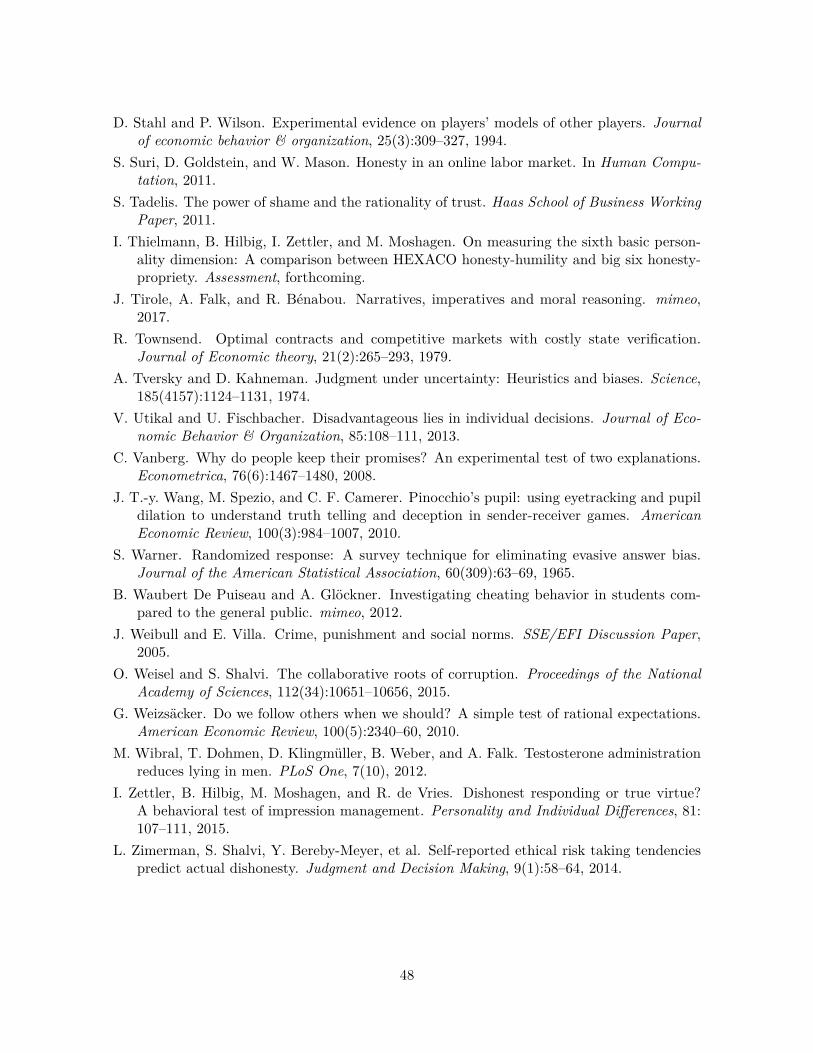
D. Stahl and P. Wilson. Experimental evidence on players’ models of other players. Journalof economic behavior & organization, 25(3):309–327, 1994.

S. Suri, D. Goldstein, and W. Mason. Honesty in an online labor market. In Human Compu-tation, 2011.

S. Tadelis. The power of shame and the rationality of trust. Haas School of Business WorkingPaper, 2011.

I. Thielmann, B. Hilbig, I. Zettler, and M. Moshagen. On measuring the sixth basic person-ality dimension: A comparison between HEXACO honesty-humility and big six honesty-propriety. Assessment, forthcoming.

J. Tirole, A. Falk, and R. Bénabou. Narratives, imperatives and moral reasoning. mimeo,2017.

R. Townsend. Optimal contracts and competitive markets with costly state verification.Journal of Economic theory, 21(2):265–293, 1979.

A. Tversky and D. Kahneman. Judgment under uncertainty: Heuristics and biases. Science,185(4157):1124–1131, 1974.

V. Utikal and U. Fischbacher. Disadvantageous lies in individual decisions. Journal of Eco-nomic Behavior & Organization, 85:108–111, 2013.

C. Vanberg. Why do people keep their promises? An experimental test of two explanations.Econometrica, 76(6):1467–1480, 2008.

J. T.-y. Wang, M. Spezio, and C. F. Camerer. Pinocchio’s pupil: using eyetracking and pupildilation to understand truth telling and deception in sender-receiver games. AmericanEconomic Review, 100(3):984–1007, 2010.

S. Warner. Randomized response: A survey technique for eliminating evasive answer bias.Journal of the American Statistical Association, 60(309):63–69, 1965.

B. Waubert De Puiseau and A. Glöckner. Investigating cheating behavior in students com-pared to the general public. mimeo, 2012.

J. Weibull and E. Villa. Crime, punishment and social norms. SSE/EFI Discussion Paper,2005.

O. Weisel and S. Shalvi. The collaborative roots of corruption. Proceedings of the NationalAcademy of Sciences, 112(34):10651–10656, 2015.

G. Weizsäcker. Do we follow others when we should? A simple test of rational expectations.American Economic Review, 100(5):2340–60, 2010.

M. Wibral, T. Dohmen, D. Klingmüller, B. Weber, and A. Falk. Testosterone administrationreduces lying in men. PLoS One, 7(10), 2012.

I. Zettler, B. Hilbig, M. Moshagen, and R. de Vries. Dishonest responding or true virtue?A behavioral test of impression management. Personality and Individual Differences, 81:107–111, 2015.

L. Zimerman, S. Shalvi, Y. Bereby-Meyer, et al. Self-reported ethical risk taking tendenciespredict actual dishonesty. Judgment and Decision Making, 9(1):58–64, 2014.

48

Online Appendices

A Further Results of the Meta Study

In this appendix, we discuss additional design details and results of the meta study including

hypotheses tests. Table A.1 provides descriptive statistics of the independent variables. Figure

A.1 marks all countries in which experiments were conducted. The world-wide coverage is

quite good, except for Africa and the Middle East.

A.1 Design

We searched in different ways for studies to include in the meta study, using Google Scholar

for direct search of all keywords used in the early papers in the literature and to trace who

cited those early papers, New Economic Papers (NEP) alerts and emails to professional email

lists. We include all studies using the FFH paradigm, i.e., in which subjects conduct a random

draw and then report their outcome of the draw, i.e., their state. This excludes sender-receiver

games as studied in Gneezy (2005) and the many subsequent papers which use this paradigm

or promise games as in Charness and Dufwenberg (2006). We require that the true state is

unknown to the experimenter but that the experimenter knows the distribution of the random

draw. The first requirement excludes studies in which the experimenter assigns the state to

the subjects (e.g., Gibson et al. 2013) or learns the state (e.g., Gneezy et al. 2013). The second

requirement excludes the many papers which use the matrix task introduced by Mazar et al.

(2008) and comparable real-effort reporting tasks, e.g., Ruedy and Schweitzer (2010). We

do include studies in which subjects report whether their prediction of a random draw was

correct or not (as in Jiang 2013). Moreover, we require that the payoff from reporting is

independent of the actions of other subjects. This excludes games like Conrads et al. (2014)

or d’Adda et al. (2014). We do allow that reporting has an effect on other subjects. We need

to know the expected payoff level, i.e., the nominal reward and the likelihood that a subject

actually receives this nominal reward. If the payoff is non-monetary, we translate the payoff

as accurately as possible into a monetary equivalent. We further require that the expected

payoff level is not constant, in particular not always zero, i.e., making different reports has

to lead to different consequences. We exclude studies in which subjects could self-select into

49

the reporting experiment after learning about the rules of the experiment. This excludes

the earliest examples of this class of experiments, Batson et al. (1997) and Batson et al.

(1999). Finally, we exclude random draws with non-symmetric distributions, except if the

draw has only two potential states. We exclude such distributions since the average report

for asymmetric distributions with many states is difficult to compare to the average report of

symmetric distributions. This only excludes Cojoc and Stoian (2014), a treatment of Gneezy

et al. (forthcoming) and two of our treatments reported in this paper.30

A.2 Influence of Treatment Variables

In this section, we further explore the effect of variables that differ between treatments and

test the statistical significance of those effects. For such treatment-level variables, we use

two complementary identification strategies. First, we can assume that the error term is

independent of the explanatory variables once we control for all observable variables. This

conditional-independence assumptions allows us to interpret the regression coefficients as the

causal effects of the explanatory variables. While the conditional-independence assumption

is usually regarded as a quite strong assumption, it is less strong in our setting for several

reasons. Economics laboratory experiments are highly standardized and lab experiments are

run with very abstract framing, usually eschewing any context and just describing the rules

of the games. Both of these arguments mean that the importance of omitted variables is

likely to be limited. Moreover, researchers usually select the design of their experiments with

regard to the research question they are interested in and not with regard to characteristics of

the local subject pool. Reverse causality is thus also unlikely. Results are reported in Table

A.2, columns 1 and 2. We include all explanatory variables that vary across more than one

treatment.31

The second identification strategy we employ makes use of the random assignment of

subjects to treatments within study (and the few within-subject experiments). As long as we

control for study fixed effects and as long as treatments within a study only differ along one

dimension, this eliminates all omitted variables. This is thus a very clean form of identification.30We adjust the distribution of standardized reports of experiments with asymmetric distributions and two

states such that the average standardized report is comparable to the one of symmetric distributions.31We restrict explanatory variables in this way since otherwise any treatment fixed effect could be an ex-

planatory variable. Given that we include 429 treatments this would become unwieldy.

50

The specifications with study-fixed effects are in Table A.2, columns 3 to 9.

Table A.1: Meta study: descriptive statistics

Mean # SubjectsTreatment-level variables

Maximal payoff from misreporting (in 2015 USD) 4.480 443901 if student subjects 0.577 443901 if repeated 0.244 443901 if online/telephone 0.273 443901 if control rolls suggested 0.283 443901 if reporting about state of mind 0.167 443901 if info about behavior of other subjects available 0.011 443901 if report reduces payoff of another subject 0.032 44390Year experiment conducted 2013.437 44390Author affiliation

1 if economics 0.758 443901 if psychology 0.212 443901 if sociology 0.030 44390

Method of randomization1 if coin toss 0.408 443901 if die roll 0.529 443901 if draw from urn 0.050 44390

True distribution1 if two outcomes non-uniform 0.122 443901 if two outcomes uniform 0.358 443901 if other uniform 0.370 443901 if bell shaped 0.150 44390

Individual-level variables

1 if female 0.478 22944Age 29.652 16205Field of study

1 if economics/management student 0.242 52841 if psychology student 0.027 52841 if other student 0.731 5284

# Decisions 270616# Subjects 44390# Treatments 429# Studies 90

Notes: The means are computed on subject level. The maximal payoff refers to the maximal nominalpayoff times the probability a subject is actually paid and is converted using PPP.

51

Figure A.1: Average report by country

Notes: The figure depicts the average standardized report per country. The darker the color, thehigher the average report. For exact country averages see Figure A.4.

The two specifications could yield different estimates for three reasons: (i) cleaner iden-

tification in the within-study specification, (ii) publication bias, and (iii) treatment effect

heterogeneity. First, if there are important omitted variables in the between-study specifi-

cation, the estimated coefficients will be biased. Omitted variables are not an issue for the

within-study specification. Second, we would expect that studies that do not find a significant

treatment effect are less likely to get published and are thus less likely to be included in our

meta study. This will bias upwards the coefficient in the within-study specification. The

between-studies specification suffers much less from this publication bias as we collect infor-

mation about variables which the original authors did not use for their publication decision.

If publication bias is important, then our between-study specification should give a better

estimate of the true coefficient than the within-study specification. Third, the within-study

estimates only use data from studies that vary the parameter of interest directly, thus restrict-

ing the sample considerably. If there is treatment effect heterogeneity, we would expect the

within-study estimate to differ from the between-study estimate. For example, the incentive

level could have a stronger effect for student samples than for non-student samples. We find

that treatment effect heterogeneity could indeed explain the difference between within-study

and between-study coefficients.32 If one is only interested in the average treatment effect,32Take the incentive level coefficient as example. The between-study coefficient is -0.005 (see below for details,

based on 429 treatments) and the within-study coefficient is 0.003 (based on 94 treatments). To test whethertreatment effect heterogeneity could explain this difference, we take the entire sample, draw 94 treatments at

52

the between-study specification is thus preferable as it reports the average effect of a larger

sample. Taken together, since we do not know with certainty how important the three reasons

are, we can only say that both estimates are informative. We thus report results of regressions

using both identification strategies. It turns out that in Table A.2, only one coefficient out

of seven is different from zero and has an opposite sign in the between- and within-study

regressions.

In the regressions, we cluster standard errors on each subject, thus treating repeated

decisions by the same subject as dependent but treating the decisions by different subjects

as independent. This is the usual assumption for experiments that study individual decision

making. This assumption is also made in basically all studies we include in the meta study.33

In the regressions relying on conditional independence, we also report a specification in column

2 which clusters on study to allow for dependencies within study. Independent of clustering,

we weight one decision as one observation in all regressions.34

Incentive level: Figure 1 showed that the level of incentives has only a very small effect

on the standardized report. The corresponding regressions are in Table A.2, columns 1 and

2. An increase of the potential payoff by 1 USD changes the standardized report by -0.005.

In column 3, we only use within-study variation for identification. We restrict the sample

to those studies which vary the payoff level between treatments. A couple of studies vary

payoff level and another variable independently. In the regression, we control for those other

variables and mark this as “Additional controls: Yes” in the table. If we cannot properly

control for within-study variation, we exclude the affected treatments (we do the same in

columns 4–9). The resulting coefficient of 0.003 is very similar to the coefficient derived under

the conditional-independence assumption. Even though the coefficients are very small, given

our large sample size, both are significantly different from zero. Taken together, this provides

converging evidence that the average amount of lying does not change much if stakes are

increased. This result is further corroborated by Figure A.2. This figure shows the distribution

random and run the between-study specification on this subsample. We repeat this process 10000 times. Wefind that 28 percent of the between-study coefficients are larger than 0.003.

33In two studies, Diekmann et al. (2015) and Rauhut (2013), subjects are shown the reports of other subjectsin their matching group before making a decision. For these studies we cluster on matching group rather thanon individual.

34If we weight by subject, results are very similar. Only the overall average standardized report is then 0.321instead of 0.234.

53

TableA.2:Regressions

oftreatm

ent-levelv

ariables

Dep

ende

ntvaria

ble:

Stan

dardized

repo

rt(1)

(2)

(3)

(4)

(5)

(6)

(7)

(8)

(9)

Max

imal

payo

fffro

mmisr

eportin

g-0.005***

-0.005

0.003***

(0.001)

(0.003)

(0.001)

1ifstud

entsubjects

0.093***

0.093**

0.100***

(0.010)

(0.043)

(0.026)

1ifrepe

ated

-0.115***

-0.115**

(0.012)

(0.053)

1ifon

line/teleph

one

-0.006

-0.006

0.027

(0.012)

(0.052)

(0.032)

1ifcontrolr

olls

suggested

0.040***

0.040

0.168***

(0.014)

(0.050)

(0.052)

1ifrepo

rtingab

outstateof

mind

0.051***

0.051

0.173***

(0.014)

(0.073)

(0.034)

1ifinfo

abou

tbe

havior

ofothe

rsubjects

available

0.043

0.043***

0.046

(0.042)

(0.012)

(0.048)

1ifrepo

rtredu

cespa

yoffof

anothersubject

-0.048***

-0.048

-0.095***

(0.015)

(0.053)

(0.017)

Year

expe

rimentcond

ucted

-0.003

-0.003

(0.002)

(0.005)

Add

ition

alcontrols

No

No

Yes

Yes

No

Yes

Yes

Yes

Yes

Autho

raffi

liatio

nFE

Yes

Yes

No

No

No

No

No

No

No

Ran

domizationmetho

dFE

Yes

Yes

No

No

No

No

No

No

No

True

distrib

utionFE

Yes

Yes

No

No

No

No

No

No

No

Cou

ntry

FEYe

sYe

sYe

sYe

sNo

No

No

No

No

Stud

yFE

No

No

Yes

Yes

Yes

Yes

Yes

Yes

Yes

#Decision

s270616

270616

51335

91593

1214

577

1200

24349

5510

#Su

bjects

44390

44390

7896

4792

906

577

1200

1642

3275

#Tr

eatm

ents

429

429

9440

1214

1622

42#

Stud

ies

9090

118

33

15

6#

Clusters

44213

907896

4792

906

577

1200

1465

3275

Notes:OLS

regressio

ns.Rob

uststan

dard

errors

clusteredon

individu

alsubjects

(onstud

iesin

column2)

arein

parenthe

ses.

The

samplein

columns

3to

7is

restric

tedto

thosestud

iesin

which

theinde

pend

entvaria

bleof

interest

varie

s.Max

imal

payofffro

mmisr

eportin

gis

the

diffe

renc

eof

thehigh

estan

dlowe

stpo

tentialp

ayoff

(con

verted

byPP

Pto

2015

USD

).The

fixed

effects

controlfor

author

affilia

tion

(econo

mics,

psycho

logy,s

ociology

),rand

omizationmetho

d(die

roll,

coin

toss,d

raw

from

urn),truedistrib

ution(asymmetric

with

two

outcom

es,u

niform

with

twoou

tcom

es,o

ther

unifo

rm,b

ells

hape

d),c

ountry

and/

orstud

y.Sign

ificanc

eat

the1,

5,an

d10

percentlevelis

deno

tedby

***,

**,a

nd*,

respectiv

ely.

54

of reports for experiments using a uniform distribution with six states (this represents about

a third of the data set). We collapse treatments by the potential payoff from misreporting

and show the distributions for the four quartiles (weighted by number of subjects). The line

marked by “1” is the distribution of the treatments with the lowest payoffs while the line

marked “4” represents the treatments with the highest payoffs. Overall, distributions do not

differ systematically by payoff level. All distributions are increasing and the second highest

state is always reported with more than 1/6 probability. Overall, neither the average report

nor the reporting pattern is affected by the payoff level.

Figure A.2: Distribution of reports by incentive level

Notes: The figure depicts the distribution of reports for treatments that use a uniform distributionwith six states and linear payoff increases. Treatments are collapsed into quartiles by the level of themaximal payoff from misreporting. The line marked by “1” is the distribution of the treatments withthe lowest payoffs while the line marked “4” represents the treatments with the highest payoffs. Thedashed line indicates the truthful distribution at 1/6.

Repetition: The regressions in Table A.2, columns 1 and 2, show that experiments

with repeated reports induce on average markedly lower reports than one-shot experiments.

There are no studies which compare one-shot with repeated implementations directly. We

can still use within-study variation to estimate the effect of repetition by comparing reports

in early vs. late rounds. Figure A.3 plots the average standardized report by treatment and

55

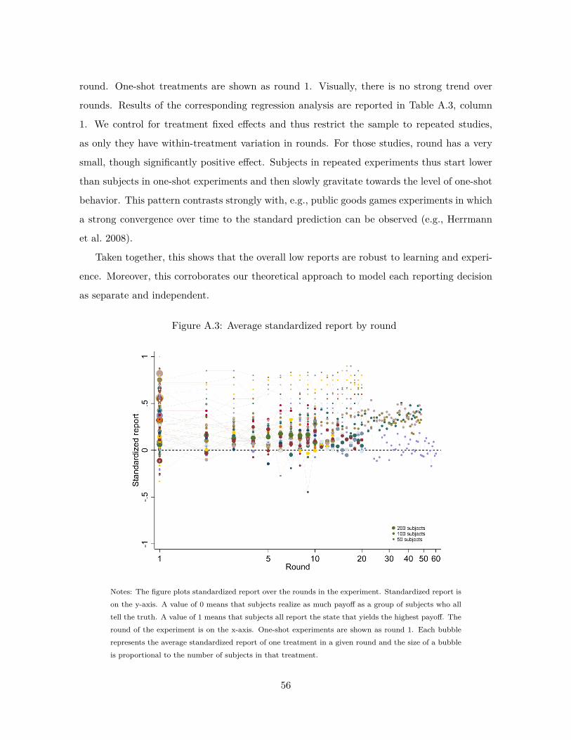
round. One-shot treatments are shown as round 1. Visually, there is no strong trend over

rounds. Results of the corresponding regression analysis are reported in Table A.3, column

1. We control for treatment fixed effects and thus restrict the sample to repeated studies,

as only they have within-treatment variation in rounds. For those studies, round has a very

small, though significantly positive effect. Subjects in repeated experiments thus start lower

than subjects in one-shot experiments and then slowly gravitate towards the level of one-shot

behavior. This pattern contrasts strongly with, e.g., public goods games experiments in which

a strong convergence over time to the standard prediction can be observed (e.g., Herrmann

et al. 2008).

Taken together, this shows that the overall low reports are robust to learning and experi-

ence. Moreover, this corroborates our theoretical approach to model each reporting decision

as separate and independent.

Figure A.3: Average standardized report by round

Notes: The figure plots standardized report over the rounds in the experiment. Standardized report ison the y-axis. A value of 0 means that subjects realize as much payoff as a group of subjects who alltell the truth. A value of 1 means that subjects all report the state that yields the highest payoff. Theround of the experiment is on the x-axis. One-shot experiments are shown as round 1. Each bubblerepresents the average standardized report of one treatment in a given round and the size of a bubbleis proportional to the number of subjects in that treatment.

56

Subject pool: Student samples report significantly higher than samples taken from

the general population. Since the latter samples are likely to also include some current

students and many subjects who used to be students, these regressions likely underestimate

the difference between students and non-students. Students and non-students differ in many

respects. We show below that the student effect is partly due to age. In addition, cognitive

skills, socio-economic background, current income, etc. could all be part of it.

Reporting channel: While most experiments were conducted in a laboratory, about a

third of experiments were conducted remotely via telephone or an online survey. Since the

experimenter controls the entire environment of the lab, subjects might fear to be observed,

say, by secret cameras. Such an observation is impossible if reports are done by telephone

or an online survey since the (physical) random draw is done remotely and thus entirely

unobservable. The channel of reporting could also have a direct effect on reporting. We find

that reports done remotely do not differ from reports in the lab.

Control rolls suggested: In about one in five experiments the experimenter suggested

explicitly that subjects use the randomization device (most often a die) several times in a

row. We find that suggesting control rolls increases reports significantly (columns 1 and 6).35

Reporting about state of mind: Following Jiang (2013) and Greene and Paxton

(2009), quite a few studies ask subjects to privately make a prediction about the outcome of

a random draw. The random draw is usually implemented on a computer and the outcome

is known to the experimenter. The report consists of the subject claiming whether their

prediction was correct or not. The overall structure is very similar to a standard coin-flip

experiment: whether the report is truthful cannot be judged individually by the experimenter,

but the experimenter knows the true distribution of states. The only difference is thus whether

the subject makes a report about a state of mind or a physical state of the world. The between-

study results in column 1 show that reporting about a state of mind leads to significantly

higher reports. The one study which tested this difference directly (Kajackaite and Gneezy35This effect could be because subjects report the highest state of all rolls they did, even though they were

instructed that only the very first roll counted for the report (Shalvi et al. 2011, Gächter and Schulz 2016c).Similarly, the control rolls could provide an excuse or narrative for the subject to report a higher state withoutfeeling too bad about it. Obviously, even if experimenters did not suggest to roll several times, subjects couldhave rolled several times and report the highest state anyway (or not roll at all and just report whatever theywanted). Perhaps subjects did not have the idea to roll several times. Or the effect is more subtle, i.e., for avalid narrative one needs an external person to suggest the control rolls.

57

2017) also finds that reports about a state of mind are significantly higher (column 7).

Information about others’ behavior: In a few experiments, subjects were given in-

formation about the past behavior of other subjects in similar experiments. This does not

affect the average report significantly, except in column 2.

From whom payoff is taken: In most experiments, subjects take money from the

experimenter or the laboratory if they report higher states. In some treatments, subjects’

reports instead reduces the payoff of another subject, i.e., the total amount of payoff allocated

to two subjects is fixed and the report decides how much of that fixed amount goes to the

reporting subject. Columns 1 and 9 indicate that this leads to a significant reduction in

reports.

Year of experiment: Reports have decreased slowly over time but this effect is very

small, given that the earliest experiments were conducted in 2005.

Author affiliation: Studies conducted by economists yield slightly higher reports than

studies conducted by psychologists. The differences to sociologists’ experiments are not sig-

nificant.

Randomization method: Reports do not differ significantly when a die roll or a coin

toss is used. Studies using a draw from an urn yield lower reports.

True distribution: Reports for different uniform distributions do not differ significantly

(see also Figure A.7). Compared to uniform distributions, asymmetric distributions have

higher reports and bell-shaped distributions have lower reports.

Country: Behavior is surprisingly robust across countries. Figure A.4 plots average

standardized reports by country. The country average is marked by a cross. Some of the

cross-country variation comes from studies that run the same design across different countries

while some of the variation is coming from researchers using convenience samples of subjects

in different countries. For those countries for which we have a decent amount of data, the

average standardized report varies only little across countries, from about 0.1 to about 0.5.

Adding country fixed effects to the regression in Column 1 of Table A.2 increases the adjusted

R2 from 0.368 to 0.455. For detailed analyses of what drives cross-country differences, see,

e.g., Pascual-Ezama et al. (2015), Hugh-Jones (2015), Mann et al. (2016) or Gächter and

Schulz (2016c).

58

Figure A.4: Average standardized report by country

Notes: The figure plots standardized report against country. Standardized report is on the y-axis. Avalue of 0 means that subjects realize as much payoff as a group of subjects who all tell the truth.A value of 1 means that subjects all report the state that yields the highest payoff. Each bubblerepresents the average standardized report of one treatment and the size of a bubble is proportionalto the number of subjects in that treatment. The cross is the average per country.

A.3 Heterogeneous Treatment Effects

So far, we have focused on variables that differed only on treatment level. For a subset of

studies we also have data on individual-level variables, namely gender, age and field of study.

Gender: Figure A.5 shows the effect of gender on reports. The majority of treatments is

below the 45° line, indicating that female subjects report lower numbers than male subjects.

However, there are also many treatments in which women report higher numbers than men.

We test the significance of this effect by regressing the report on a gender dummy and con-

trolling for treatment fixed effects. We thus only use within-treatment variation. The results

are presented in Table A.3, column 2: women’s standardized report is on average 0.058 lower

than men’s. This effect is highly significant. Figure A.6 shows the distribution by gender of

all treatments that use a uniform distribution with six states for which we have gender data.

Men are generally less likely to report lower states and more likely to report higher states.

59

Figure A.5: Average standardized report by gender

Notes: The figure plots the average standardized report of male subjects (x-axis) vs. the averagestandardized report by female subjects (y-axis). A standardized report of 0 means that subjectsrealize as much payoff as a group of subjects who all tell the truth. A value of 1 means that subjectsall report the state that yields the highest payoff. Data is restricted to those treatments where maleand female subjects participated. The size of a bubble is proportional to the number of subjects inthat treatment.

60

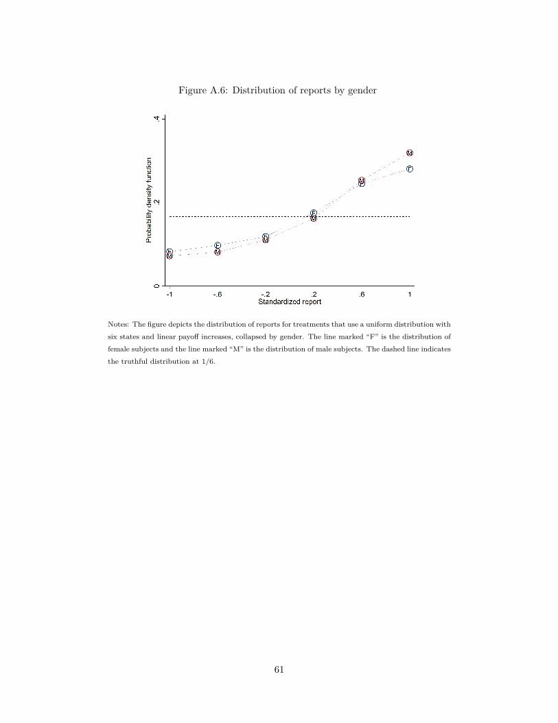
Figure A.6: Distribution of reports by gender

Notes: The figure depicts the distribution of reports for treatments that use a uniform distribution withsix states and linear payoff increases, collapsed by gender. The line marked “F” is the distribution offemale subjects and the line marked “M” is the distribution of male subjects. The dashed line indicatesthe truthful distribution at 1/6.

61

Table A.3: Regressions of individual-level variables

Dependent variable: Standardized report

(1) (2) (3) (4) (5)Round 0.001**

(0.000)1 if female -0.058***

(0.009)Age -0.002*** -0.004

(0.001) (0.003)Age squared 0.000

(0.000)1 if economics/management student 0.005

(0.022)1 if psychology student -0.062

(0.078)Treatment FE Yes Yes Yes Yes Yes# Decisions 73582 88503 39828 39828 8335# Subjects 4862 22172 15472 15472 4655# Treatments 43 239 144 144 52# Studies 11 47 33 33 9# Clusters 4806 22116 15472 15472 4655

Notes: OLS regressions. Robust standard errors clustered on individual subjects are in parentheses.The sample in each specification is restricted to those treatments in which the independent variable(s)vary. Significance at the 1, 5, and 10 percent level is denoted by ***, **, and *, respectively.

Age: Older subjects tend to report lower numbers. This effect is significant in a linear

regression but not significant when we add age squared (Table A.3, columns 3 and 4).

Field of study: While students in general make higher reports than non-students, we do

not find an effect of field of study (Table A.3, column 5).

A.4 Further Robustness Checks

Other uniform distributions: In Figure 2, we showed for uniform distributions with two

and six states that the distribution of reports is increasing and has support on more than

62

one state (it actually has almost always full support). This finding generalizes to uniform

distributions with different number of states. Figure A.7 demonstrates that the distribution

of reports is actually quite similar for experiments with different numbers of states. We

observe over-reporting of non-maximal states for the six- and ten-state distributions. The

general pattern of reporting across the four distributions in the graph suggests that we should

expect such over-reporting to occur for any uniform distribution with more than three states.

Figure A.7: Distribution of reports (uniform true distributions)

Notes: The figure depicts the difference between the actual and the truthful distribution of reports fortreatments that use a uniform true distribution and linear payoff increases. Treatments are collapsedby the number of states, 2, 3, 6, or 10. The dashed line at 0 indicates the truthful distribution. Thesize of a bubble is proportional to the number of subjects in the treatments with a given number ofstates.

Individual-level analysis: Up to here, we have shown that reporting is far from the

standard rational prediction of a standardized report of +1 in the entire sample and in all

sub-groups defined by observable characteristics, e.g., gender. However, maybe there is a

sub-group, which we cannot identify by observable variables, which does behave according to

the standard prediction. For this we would need to identify for each individual whether they

lied or not, which is not possible for the one-shot experiments. However, if we aggregate the

many reports of an individual subject in repeated experiments, we can test for each individual

63

subject whether their sequence of reports could be generated by truth-telling. In particular,

it is increasingly unlikely to repeatedly draw the highest-payoff state. Note that we depart for

this analysis from our usual approach of treating each decision as separate and independent.

For example, if subjects care about being perceived as truthful, the predicted behavior depends

on whether subjects and the audience player treat each decision separately or not. In Figure

A.8 we focus on experiments in which subjects repeatedly report the state they drew of a

uniform distribution with two states and add up the number of times a subject reported the

high-payoff state. To make experiments with different numbers of rounds comparable, we

plot the share of the potential high-payoff reports on the x-axis and the difference between

the observed distribution and the truthful binomial distribution on the y-axis. Reporting

the highest-payoff state in each round is the standard rational prediction. This reporting

pattern could have resulted from truth-telling only with a minuscule chance of 1/210 to 1/240.

As one can see in the figure, more subjects always report the high-payoff state than would

be expected under full truth-telling. However, the overall share of subjects at this point is

surprisingly small. Only 3.6 percent of subjects always report the high-payoff state and only

6.7 percent report it more than 80 percent of the time (the size of the bubbles is proportional

to the number of subjects making the respective report). Overall, this suggests that also

individually, people are far from the standard prediction.

64

Figure A.8: Distribution of sum of reports (repeated reports of two-state distributions)

Notes: The figure displays the distribution of the sum of standardized reports in experiments in whichsubjects repeatedly report the state of a uniform distribution with two states.. Each line representsone treatment. The share of the potential high-payoff reports is on the x-axis. On the y-axis is thedifference between the actual and the truthful PDF. The size of a bubble is proportional to the numberof subjects in a given treatment at this share of high-payoff reports.

65

A.5 List of Studies Included in the Meta Study

Table A.4: List of studies included in the meta study

Study # treatments # subjects Country Randomization method True distributionthis study * 7 1124 United Kingdom multiple multipleAbeler et al. (2014) * 4 1102 Germany coin toss multipleAbeler (2015) * 1 60 China draw from urn 1D10Abeler and Nosenzo (2015) * 9 507 Germany draw from urn 1D10Amir et al. (2016) * 11 403 Israel coin flip 20D2Antony et al. (2016) * 2 200 Germany die roll 1D6Arbel et al. (2014) * 2 399 Israel die roll 1D6Ariely et al. (2014) 1 188 Germany die roll 1D6Aydogan et al. (forthcoming) 2 120 Germany coin toss 2D2Banerjee et al. (2016) * 16 672 India die roll 1D6Barfort et al. (2015) 1 862 Denmark die roll asy. 1D2Basic et al. (2016) * 3 272 Germany die roll 1D6Beck et al. (2016) * 6 128 Germany die roll 1D6Blanco and Cárdenas (2015) 2 103 Colombia die roll 1D6Braun and Hornuf (2015) 7 342 Germany die roll 1D2Bryan et al. (2013) * 3 269 USA coin toss 1D2Bucciol and Piovesan (2011) * 2 182 Italy coin toss 1D2Cadsby et al. (2016) 1 90 China die roll 1D6Cappelen et al. (2016) * 2 1473 Tanzania coin toss 6D2Charness et al. (2017) 4 338 Spain die roll 1D10Chytilova and Korbel (2014) * 1 117 Czech Republic die roll 1D6Clot et al. (2014) * 2 98 Madagascar die roll 1D6Cohn et al. (2014) * 8 563 coin toss 1D2Cohn et al. (2015) * 4 375 Switzerland coin toss 1D2Cohn and Maréchal (forthcoming) 1 162 Switzerland coin toss 1D2Cohn et al. (2016) 4 468 Switzerland coin toss 1D2Conrads et al. (2013) * 4 554 Germany die roll 1D6Conrads and Lotz (2015) * 4 246 Germany coin toss 4D2Conrads et al. (2017) 1 114 Germany die roll 1D2Dai et al. (forthcoming) 2 384 France die roll 1D3Dato and Nieken (2015) 1 288 Germany die roll 1D6Dieckmann et al. (forthcoming) 5 1015 multiple (5) coin toss 1D2Diekmann et al. (2015) * 4 466 Switzerland die roll 1D6Di Falco et al. (2016) 1 1080 Tanzania coin toss 1D2Djawadi and Fahr (2015) 1 252 Germany draw from urn asy. 1D2Drupp et al. (2016) 4 170 Germany coin toss 4D2Duch and Solaz 3 3400 multiple (3) die roll 1D6Effron et al. (2015) * 8 2151 USA coin toss 1D2Fischbacher and Föllmi-Heusi (2013) * 5 979 Switzerland die roll 1D6Foerster et al. (2013) * 1 28 Germany die roll 12D8Fosgaard (2013) * 1 505 Denmark die roll 2D6Fosgaard et al. (2013) * 4 209 Denmark coin toss 1D2

66

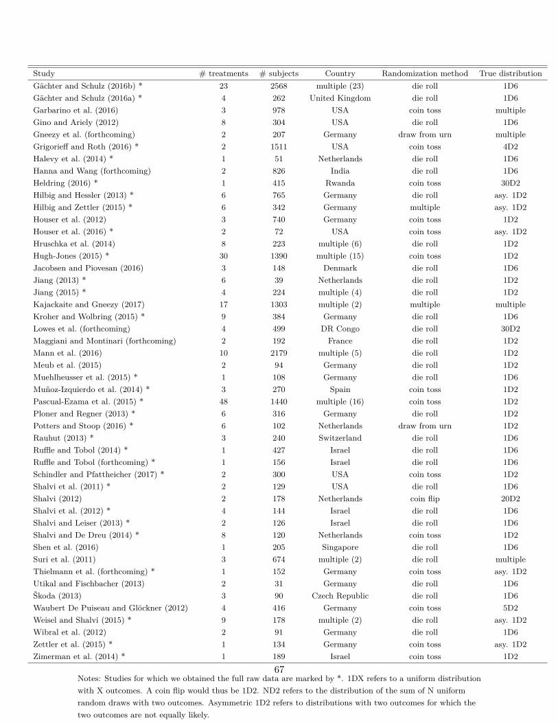
Study # treatments # subjects Country Randomization method True distributionGächter and Schulz (2016b) * 23 2568 multiple (23) die roll 1D6Gächter and Schulz (2016a) * 4 262 United Kingdom die roll 1D6Garbarino et al. (2016) 3 978 USA coin toss multipleGino and Ariely (2012) 8 304 USA die roll 1D6Gneezy et al. (forthcoming) 2 207 Germany draw from urn multipleGrigorieff and Roth (2016) * 2 1511 USA coin toss 4D2Halevy et al. (2014) * 1 51 Netherlands die roll 1D6Hanna and Wang (forthcoming) 2 826 India die roll 1D6Heldring (2016) * 1 415 Rwanda coin toss 30D2Hilbig and Hessler (2013) * 6 765 Germany die roll asy. 1D2Hilbig and Zettler (2015) * 6 342 Germany multiple asy. 1D2Houser et al. (2012) 3 740 Germany coin toss 1D2Houser et al. (2016) * 2 72 USA coin toss asy. 1D2Hruschka et al. (2014) 8 223 multiple (6) die roll 1D2Hugh-Jones (2015) * 30 1390 multiple (15) coin toss 1D2Jacobsen and Piovesan (2016) 3 148 Denmark die roll 1D6Jiang (2013) * 6 39 Netherlands die roll 1D2Jiang (2015) * 4 224 multiple (4) die roll 1D2Kajackaite and Gneezy (2017) 17 1303 multiple (2) multiple multipleKroher and Wolbring (2015) * 9 384 Germany die roll 1D6Lowes et al. (forthcoming) 4 499 DR Congo die roll 30D2Maggiani and Montinari (forthcoming) 2 192 France die roll 1D2Mann et al. (2016) 10 2179 multiple (5) die roll 1D2Meub et al. (2015) 2 94 Germany die roll 1D2Muehlheusser et al. (2015) * 1 108 Germany die roll 1D6Muñoz-Izquierdo et al. (2014) * 3 270 Spain coin toss 1D2Pascual-Ezama et al. (2015) * 48 1440 multiple (16) coin toss 1D2Ploner and Regner (2013) * 6 316 Germany die roll 1D2Potters and Stoop (2016) * 6 102 Netherlands draw from urn 1D2Rauhut (2013) * 3 240 Switzerland die roll 1D6Ruffle and Tobol (2014) * 1 427 Israel die roll 1D6Ruffle and Tobol (forthcoming) * 1 156 Israel die roll 1D6Schindler and Pfattheicher (2017) * 2 300 USA coin toss 1D2Shalvi et al. (2011) * 2 129 USA die roll 1D6Shalvi (2012) 2 178 Netherlands coin flip 20D2Shalvi et al. (2012) * 4 144 Israel die roll 1D6Shalvi and Leiser (2013) * 2 126 Israel die roll 1D6Shalvi and De Dreu (2014) * 8 120 Netherlands coin toss 1D2Shen et al. (2016) 1 205 Singapore die roll 1D6Suri et al. (2011) 3 674 multiple (2) die roll multipleThielmann et al. (forthcoming) * 1 152 Germany coin toss asy. 1D2Utikal and Fischbacher (2013) 2 31 Germany die roll 1D6Škoda (2013) 3 90 Czech Republic die roll 1D6Waubert De Puiseau and Glöckner (2012) 4 416 Germany coin toss 5D2Weisel and Shalvi (2015) * 9 178 multiple (2) die roll asy. 1D2Wibral et al. (2012) 2 91 Germany die roll 1D6Zettler et al. (2015) * 1 134 Germany coin toss asy. 1D2Zimerman et al. (2014) * 1 189 Israel coin toss 1D2

Notes: Studies for which we obtained the full raw data are marked by *. 1DX refers to a uniform distributionwith X outcomes. A coin flip would thus be 1D2. ND2 refers to the distribution of the sum of N uniformrandom draws with two outcomes. Asymmetric 1D2 refers to distributions with two outcomes for which thetwo outcomes are not equally likely.

67

B Additional Models

In this section we discuss the remaining models listed in Table 1. All proofs are in Appendix

E.

B.1 Inequality Aversion

This model captures the widely discussed notion that individuals care about how their mone-

tary payoff compares to the payoff of others as in, e.g., Fehr and Schmidt (1999) or Bolton and

Ockenfels (2000). In our formal model we will build off the intuition of the latter, although

similar results hold for a model in line with the former. We suppose that individuals care not

just about their own payoff, but also the average payoff (and so our solution concept is the

standard Bayes’ Nash Equilibrium).36 Formally, utility is

φ(r, ς(r − r); θIA)

where r is the mean report. ς is a function that maps the difference between an individual’s

payoff and the average payoff to a utility cost. It has a minimum at 0 and is increasing in

the absolute distance from 0 of its argument. The only element of ~θ that affects utility is

the scalar θIA which governs the weight that an individual applies to social comparisons.

We suppose that φ is strictly increasing in its first argument and decreasing in its second

(strictly so when θIA>0), i.e., individuals like money and dislike inequality, and is decreasing

in θIA; and that the cross partial of φ with respect to the second argument and θIA is strictly

negative. An equilibrium will exist because of the continuity of φ and ς and the property

that r is continuous in the threshold types (where the threshold is in θIA). Because of the

dependence of any given individual’s optimal reports on others’ reports, there may be multiple

equilibria. For example, if all individuals face a sufficiently strong cost of deviation from the

mean report, then for any report r, everyone reporting r is an equilibrium.

Observation 1 Suppose individuals have Inequality Aversion utility. For arbitrary n, we36This model can also capture a notion of a preference for conformity in actions. In this model individuals

may receive a payoff from how closely their action matches other’s actions. Because, in this model, an actiondirectly maps to a monetary payoff, caring about the average action of others is the same as caring about theaverage payoff of others.

68

have f -invariance, affinity, o-invariance and potentially lying down when the state is unob-

served or observed.

B.2 Inequality Aversion + LC

We extend the simple inequality aversion model we develop in Section B.1, so that individuals

additionally care about the cost of lying (for an early version of such a model, see Hurkens

and Kartik 2009). Formally, utility is

φ(r, ς(r − r), c(r, ω); θIA, θLC)

where r is the mean report. The function ς has the same properties as in the inequality

aversion model. The function c has the same properties as in the LC model. The only

elements of ~θ that affect utility are the scalars θIA and θLC which govern the weight that

an individual applies to social comparison and lying costs. We suppose that φ is strictly

increasing in its first argument, decreasing in its second (strictly so when θIA > 0), decreasing

in its third (strictly so when θLC > 0), and is decreasing in θIA and θLC . Moreover, as before,

the partial of φ with respect to ς and θIA is strictly negative and the partial with respect to

c and θLC is strictly negative. As in the inequality aversion model, an equilibrium will exist

because of the continuity of φ, c and ς and the property that r is continuous in the threshold

types, but because of the dependence of payoffs on others’ reports, there may be multiple

equilibria.

Observation 2 Suppose individuals have Inequality Aversion + LC utility. For arbitrary n,

we have no prediction with regard to shifts in F , affinity, o-invariance and potentially lying

down when the state is unobserved or observed. For n = 2, the Inequality Aversion + LC

model exhibits drawing in when the equilibrium is unique.

B.3 Censored Conformity in Lying Costs

This section presents a variation of the CLC model. One could imagine that an individual

does not normalize their lying cost by the average lying cost in society (as in CLC), but only

by the lying costs incurred by individuals who “could have” lied profitably, i.e., those who

69

did not receive the maximal draw. As in in the CLC model, payoffs thus depend on others’

strategies; and so we use the framework that Battigalli and Dufwenberg (2009) developed for

psychological games.

In this model, as in CLC, individuals will not want to lie downwards. We denote, supressing

extraneous notation, the average lying costs of all those who do not draw the maximal state

as cω 6=ωn . The utility function is then:

φ(r, η(c(r, ω), cω 6=ωn); θCCLC)

where η is the normalized cost function. η is falling in the first argument and increasing

in the second. We suppose that η(0, cω 6=ωn) = 0. φ is strictly increasing in the first argument,

falling in the second (strictly when θCCLC > 0), and falling in θCCLC . Last, the cross partial

of φ with respect to η and θCCLC is strictly negative. An equilibrium will exist because of the

continuity of φ, η and c (and the continuity of cω 6=ωn in the proportion of liars), but because

of the dependence of payoffs on others’ strategies, it may not be unique.

Observation 3 Suppose individuals have Censored Conformity in Lying costs utility. For

arbitrary n, we have no prediction regarding shifts in F or in G, o-invariance and no lying

down when the state is unobserved or observed. For n = 2, the Censored CLC model exhibits

f -invariance and affinity.

B.4 Reputation for Being Not Greedy

Individuals often want to signal to the audience about a particular characteristic they pos-

sess. We use as an inspiration the motivations provided in Bénabou and Tirole (2006) and

Fischbacher and Föllmi-Heusi (2013), and model an individual as wanting to signal to the

audience that they are not greedy, i.e., they place a relatively low value on money compared

to reputation. Thus, an individual’s utility will depend on the audience’s beliefs about their

type and the scalar θRNG(the only element of ~θ that affects utility), which is unobserved.

However, the belief can be conditioned on the report r itself. Because utility depends on the

audience’s beliefs, we must use the psychological game theory framework of Battigalli and

Dufwenberg (2009) to analyze the game. Since the audience player understands the equilib-

rium strategies of all types, and correctly utilizes Bayesian updating, we can simply describe

their belief as E(θRNG|r). Given this, utility is:

70

φ(r, E(θRNG|r); θRNG)

We assume φ is increasing in the first element, i.e., individuals like money; but the partial of

φ with respect to the first element is equal to 0 when θRNG = κRNG, and otherwise strictly

positive for θRNG < κRNG. φ is also increasing in the second element, i.e., individuals like

the audience to have a high belief about their θRNG; specifically the partial of φ with respect

to the second element is 0 when θRNG = 0 and is strictly positive for θRNG > 0. Moreover,

φ is falling in θRNG, and the cross partial of φ with respect to the first element and θRNG

is strictly negative. This captures the property that individuals face both a higher benefit,

and a higher marginal benefit, of the monetary payoff when θRNG is smaller. Moreover, the

cross partial of φ with respect to the second element and θRNG is strictly positive. This

captures the property that individuals with higher θRNGs have both a higher benefit, and a

higher marginal benefit, of being perceived as having a higher expected θRNG. Intuitively our

assumptions are tantamount to supposing that less “greedy” individuals also care more about

being thought of as less greedy. Equilibrium will exist because of the continuity of φ and the

expectations operator, but may not be unique.

Observation 4 Suppose individuals have Reputation for Being Not Greedy utility. For ar-

bitrary n, we have f -invariance, no prediction regarding shifts in G, o-invariance and lying

down when the state is unobserved or observed.

B.5 LC-Reputation

Rather than caring about the reputation of having reported truthfully conditional on their

report, individuals may instead want to cultivate a reputation as a person who has high lying

costs, i.e., they like the audience to have a high belief about their θLC . Such a model is

similar to the one discussed in Frankel and Kartik (2016). It is also similar in spirit, although

in an entirely different domain, to the models of fairness by Levine (1998), Bénabou and

Tirole (2006), Ellingsen and Johannesson (2008), Andreoni and Bernheim (2009), Tadelis

(2011), and Grossman (2015). In those models individuals like to be perceived as fair as well

as actually having preferences for fairness. Thus, an individual’s utility will depend on the

audience player’s beliefs about their type, the scalar θLC , which is unobserved. However, the

belief can be conditioned on the report r itself. Because utility depends on the audience’s

71

beliefs, we use the psychological game theory framework of Battigalli and Dufwenberg (2009)

to analyze the game. Since the audience understands the equilibrium strategies of all types,

and correctly utilizes Bayesian updating, we can simply describe their belief as E(θLC |r).

Utility is

φ(r, c(r, ω), E[θLC |r]; θLC , θRep)

The only elements of ~θ that affect utility are θLC and θRep. c and θLC have the same interpre-

tation as in the LC model, and the assumptions regarding them are the same. θRep represents

the weight that any given individual places on the audience’s belief about θLC . φ is increasing

in E[θLC |r] (strictly so when θRep>0) and in θRep. The interpretation is that individuals have

a positive utility from others believing that they have high lying costs. Moreover the cross

partial of φ with respect to E[θLC |r] and θRep is strictly positive. Equilibrium will exist be-

cause of the continuity of φ, c and the expectations operator, but may not be unique because

of the dependence of payoffs on others’ strategies (via the audience’s beliefs).

Observation 5 Suppose individuals have LC-Reputation utility. For arbitrary n, we have no

predictions regarding shifts in F or in G, o-shift and potential lying down when the state is

unobserved or observed.

B.6 Guilt Aversion

Guilt aversion (Charness and Dufwenberg 2006; Battigalli and Dufwenberg 2007, 2009) is a

psychological game theory model that has been widely used to understand how individuals

report in sender-receiver games. In applying guilt aversion to our setting, we assume that

subjects experience guilt (and so lower utility) to the extent that they belief they disappointed

the audience player (i.e., report more than expected), for example, the experimenter. Because

beliefs are correct in equilibrium, the audience expects the report to be the average report

induced by the equilibrium G, which we denote r (each equilibrium will have an associated r).

To keep notation simple, we suppress the fact that r is an equilibrium object that depends on

F and H and the selected equilibrium. 37 Because individuals’ utility depends on the beliefs37One might argue that guilt aversion is not appropriate for this subject-experimenter interaction (or more

generally, subject-audience interaction). We still include it in our list of models since it has been widely appliedand we want our study to be able to link to that literature. Moreover, in almost a dozen experiments surveyedin the meta study (Appendix A), a higher report reduces the payoff of another subject (and not the budget of

72

of the audience, this model explicitly uses the tools of psychological game theory (Battigalli

and Dufwenberg 2007, 2009). Utility is:

φ(r, γ(r − r); θGA)

where γ is the function that maps the difference between any given individual’s report

and the average report to a utility cost. Given an equilibrium and associated r, if r ≤ r, then

γ(r− r) = 0. If r > r, then γ(r− r) is strictly increasing in r− r. The only element of ~θ that

affects utility is the scalar θGA which governs the weight that an individual applies to guilt.

We suppose that φ is strictly increasing in its first argument, decreasing it its second (strictly

so when θGA>0), decreasing in θGA, and the cross partial of the second argument and θGA is

strictly negative.

Equilibrium existence follows from the continuity of φ and γ and r. However, there may

be multiple equilibria. For example, if the audience expects that the only report given will be

the maximal report, then players will not believe that the audience will be disappointed when

the maximal report is made. Thus no one feels guilt when making the maximal report, and so

everyone makes that report. This forms an equilibrium. In contrast, if the audience expects

that the only report given will be the minimal report, then the audience will be disappointed

when any other report is made. So long as individuals experience enough guilt, it can also

be an equilibrium for everyone to then make the minimal report. However, as we formalize

below, the set of equilibria doesn’t shift with F .38

Observation 6 Suppose individuals have Guilt Aversion utility. For arbitrary n, we have

f -invariance, affinity, o-invariance and potentially lying down when the state is unobserved

or observed.the experimenter). In those treatments, guilt aversion could well be applied to the subject-subject interaction.Average behavior in these treatments is not very far away from behavior in subject-experimenter treatments(see Table A.2), so it could well be that similar motives play a role in the subject-experimenter interaction.

38Surprisingly, in our simple environment with our particular modeling assumptions, guilt aversion turnsout to predict the same as the inequality aversion model, albeit for very different underlying reasons. Theassumption about utilities when r ≤ r is different but this does not affect the predictions.

73

B.7 Choice Error

One potential explanation for the observed pattern of non-maximal reports is that individual’s

utility function only incorporates material payoffs, but individuals simply make mistakes when

choosing, and so sometimes do not actually make the utility-maximizing report. The related

Luce (1959) and McFadden et al. (1973) models of discrete choice with errors are very common

specifications. This is a non-utility based framework, as it supposes that individuals have a

standard utility function, but make errors when taking their action. Specifically, the utility

of report r is φ(r) where φ is a positive function strictly increasing in r, i.e., every individual

prefers to make the highest report. However, individuals do not always choose the utility

maximizing report. Instead, the probability of choosing report ri is eφ(ri)θCE∑n

j=1 eφ(rj)θCE . θCE is

a parameter that governs the amount of “randomness” for a given individual. As θCE goes

to infinity, the individual always chooses the utility maximizing report. As θCE goes to 0,

reports are made with uniform chance.39

Observation 7 Suppose individuals’ choices follow the choice error model. For arbitrary n,

we have f -invariance, g-invariance, o-invariance and lying down when the state is unobserved

or observed.

B.8 Kőszegi-Rabin + LC

Kőszegi and Rabin (2006) suggest a widely used model of expectations dependent reference-

dependence in which the recent rational expectations serves as the reference point. We can

combine the intuition of the Kőszegi-Rabin model with the lying cost model. Garbarino et al.

(2016), in a concurrent paper, suggest and test a related model. We suppose that individuals

face lying costs and experience gain-loss utility both over monetary outcomes, and over the

lying costs (possibly to different degrees). As before we will denote the cost of reporting r if

ω is the state as c(r, ω) which has the same properties as described under LC. The utility of

reporting r if ω is the state is then39To bring this model in line with our general theoretical framework outlined in Section 2, which is based

on error-free utility maximization, one could interpret the choice error as coming from a shock to φ(r) whichmakes a subject prefer a particular non-maximal report. This shock would be distributed such that the choiceprobabilities are as in the formula in the text.

74

φ(r, ω, a; θLC , θLAweight, θLAmoney, θLAcost) = φ(r, c(r, ω); θLC) +

θLAweight[∑k θLAmoneyI|(u(r)−u(a(ωk)))|f(ωk)+∑

k θLAcostI|(c(a(ωk), ωk)−c(a(ω), ω))|f(ωk)]

Four elements of ~θ affect utility in this model. θLC parameterizes the cost of lying.

θLAweight parametrizes the weight on gain-loss utility, and θLAmoney and θLAcost represent

the separate gain-loss parameters for money and lying costs. θLAmoneyI and θLAcostI are indi-

cator functions that take on values of 1 if the argument inside the attached absolute value is

positive, and θLAmoney or θLAcost respectively otherwise. φ takes on all the attributes that φ

does in the LC model, and c has the exact same properties. A personal equilibrium a is a map-

ping such that if a maps ω to r, then the argmax of φ(r, ω, a; θLC , θLAweight, θLAmoney, θLAcost)

is r. A personal equilibrium will exist for the reasons outlined in Kőszegi and Rabin (2006)

and Kőszegi and Rabin (2007). Morover, as pointed out by those papers, there may be mul-

tiple personal equilibria mappings a. However, there will generically be a unique preferred

personal equilibrium, i.e., an equilibrium mapping a that gives the highest utility, among all

possible equilibrium as for any given value of θLAmoney and θLAcost. We will suppose, in line

with Kőszegi and Rabin (2006) and Kőszegi and Rabin (2007), that individuals choose the

preferred personal equilibrium. Then the aggregate distribution of reports is simply the set

of reports generated by the distribution of states and as that each individual uses.40

Observation 8 Suppose individuals have Kőszegi-Rabin+LC utility. For arbitrary n, we have

no predictions regarding shifts in F , g-invariance, o-invariance and no lying down when the

state is unobserved or observed.

40As Kőszegi and Rabin (2007) point out, such an a will exist so long as we allow the action space to beconvex, i.e., allow randomization.

75

C Models that do not Match the Findings of the Meta Study

C.1 Standard Model and Lexicographic Lying Costs

The typical assumption in economics is that in anonymous, one-shot interactions, individuals

will simply maximize material payoffs, so utility is only a function of r:

φ(r)

where utility is (strictly) increasing in r. This model cannot explain the findings of the

meta study.41

Observation 9 Suppose individuals have standard utility. Then all individuals give the high-

est report.

This observation contradicts Finding 2 of the meta study. Several papers (e.g., Demichelis

and Weibull 2008, Ellingsen and Östling 2010, Kartik et al. 2014b) assume that individuals

have weak (or lexicographic) preferences for truth-telling, i.e., individuals care about r and

receive an additional small utility ε > 0 when they report truthfully. Since reports in our

setup always yield different monetary payoffs, this model makes the same predictions as the

standard model.

C.2 Reputation for Honesty (RH)

Many authors have found it plausible that individuals care about some kind of reputation

that is linked to the belief of the audience player about whether the individual reported

truthfully, where the audience can only observe the report but not the true state. Individuals

suffer a disutility from the stigma of being perceived as a liar. One might imagine that this

“stigmatization aversion” is the sole reason motivating an aversion to lying. Thus, this type of

model is like the RH+LC model described in the body of the paper, but where θLC is always

0. Therefore, an aversion to lying is motivated solely by concerns about the beliefs of the41Moreover, the standard model predicts f -invariance, g-invariance, o-invariance, and no lying down when

the state is unobserved or observed.

76

audience. As before, because the audience’s beliefs enter the utility of subject, understanding

such a model requires using the framework of Battigalli and Dufwenberg (2009). Dufwenberg

and Dufwenberg (2017) introduce a similar model, but where others’ beliefs about the size of

the lie matters for utility.

We find that such a model cannot explain the findings of the meta study. Formally, we

suppose that in a Reputation for Honesty (RH) model individuals’ utility is

φ(r,Λ(r); θRH)

Λ(r) is the fraction of liars and, as in the RH+LC model, is the audience player’s belief

about whether an individual reporting r is a liar. The only element of ~θ that affects utility

is the scalar θRH which governs the weight that an individual applies to the stigma of being

perceived as a liar. We assume φ is strictly increasing in its first argument and decreasing in

the second argument; strictly when θRH > 0. These assumptions capture the property that

individuals prefer a higher monetary payoff but dislike being thought of as a liar. Moreover, we

suppose that φ is decreasing in θRH fixing the first two arguments, and that the cross partial

of φ with respect to Λ(r) and θRH is strictly negative. An equilibrium will exist because of

standard continuity arguments, but because of the dependence of payoffs on other’s strategies

(via the audience’s beliefs) it may not be unique.

In order to understand the results, we first provide some intuition for a setting with two

states. RH predicts that, because utility depends only on reports but not on the drawn

state, individuals’ best response function will depend only on their individual θRH , not on

the drawn state. This means that conditional on having the same θRH , individuals drawing

the low or the high state will make the same report. Thus, in any equilibrium that features

full support, some individuals must lie downwards. Observe that starting with an equilibrium

with full support, there is an indifferent type: an individual who is indifferent between the

high and low reports. Everyone with a lower θRH gives the high report; everyone with a

higher θRH gives the low report. The probability of being less than the indifferent type is

H(θRH), where θRH is the indifferent type. Thus the fraction of liars at the high report is

Λ(r2) = H(θRH)f(ω1)H(θRH)f(ω1)+H(θRH)[1−f(ω1)] = f(ω1). Similarly, we can show that Λ(r1) = f(ω2).

This implies directly that if f(ω1) ≤ f(ω2) then in an equilibrium with full support the

77

fraction of liars at r2 would be weakly smaller than the fraction of liars at r1. And so

by saying r2, individuals would receive both a higher monetary payoff and a weakly lower

reputational cost. Thus, all individuals should say r2 and there cannot be an equilibrium

with full support, contradicting Finding 2 (when restricted to binary states) of the meta

study. This result generalizes to a setting with many states as we show in the proof.42

Observation 10 Suppose individuals have RH utility and F is uniform. Then all individuals

give the same report.

Because the audience player makes inferences about whether an individual lies, the re-

sults depend crucially on equilibrium reasoning (using psychological game theory). A natural

question to ask is what happens if we suppose individuals are less than fully strategically

sophisticated. In the working paper version of this paper (Abeler et al. 2016) we consider

variants of the RH model where individuals may lack strategic sophistication: they may be

k-level reasoners (as first discussed by Stahl and Wilson (1994)) or exhibit cursedness (Eyster

and Rabin 2005). These models yield the same result as the RH model.

C.3 Audit Model

The Audit model builds on the intuition of the RH model but with a twist. Individuals’

utility depends on the beliefs of the audience about whether they are a liar or not, but only

in the circumstance that they actually lied up. The model builds on the intuition of audits:

individuals fear to be “found out” as liars. The probability of being found out depends on the

report. Individuals who give a report where there are many liars are more likely to be found

out as a liar. This may be a concern about an actual audit or, our preferred interpretation,

a more metaphorical audit: individuals care about the belief of the audience player about

whether they reported truthfully – but only if they lied up. If they were honest or lied down,

they have a “clean conscience”, even though they won’t be able to prove their honesty by

showing their true state. If the audit is an actual concern about the researcher, then one can

alleviate such concerns, e.g., by conducting the experiment over the phone. Our meta study,

however, finds no difference in behavior when the experiment is conducted remotely (see Table42Moreover, the RH model predicts (for n = 2) drawing in, g-invariance, o-shift, lying down when the state

is unobserved, and no lying down when the state is observed.

78

A.2). Townsend (1979) discusses wanting to avoid detection, which could be motivated by not

wanting to be in a category which is likely populated by many liars. Kajackaite and Gneezy

(2017) also discuss such an intuition for lying aversion. Because utility (potentially) depends

on the audience player’s belief we again use the framework of Battigalli and Dufwenberg

(2009). Moreover, because the audience’s beliefs in equilibrium must be correct, we can

represent them as Λ(r).

Using the audit intuition, individuals are “investigated” with a probability that is increas-

ing in the audience’s belief that they lied, which in equilibrium, is equal to Λ(r), i.e., the

proportion of liars that report the same r as the individual. If an individual is investigated,

and discovered to have been lying upwards they face a utility cost (we suppose here that it

is a fixed cost, but with binary states it is equivalent to supposing the cost depends on the

size of the lie). Individuals face no cost if they are discovered to have lied downwards or have

been honest. Individuals’ utility function is

φ(r, Ir>ωΛ(r); θAud)

where Ir>ω is an indicator function which equals 1 if the individual lied upwards, and

0 if the individual did not lie upwards. Λ(r) is the fraction of liars at r, which is in turn

the posterior belief of the audience about the probability the individual has lied. The only

element of ~θ that affects utility is θAud which governs the weight that an individual applies to

the reputational cost. We assume that φ is strictly increasing in the first argument, decreasing

in the second argument, strictly so if θAud > 0, and decreasing in θAud. Similarly to previous

models, the cross partial of the second argument and θAud is strictly negative. An equilibrium

will exist because of standard continuity arguments, but because of the dependence of payoffs

on others’ strategies (via the audience’s beliefs) it may not be unique.

The model fails to capture the findings of the meta study because under some circum-

stances it predicts that only one report is made with positive probability in equilibrium,

contradicting Finding 2.43

Observation 11 Suppose individuals have Audit utility. Then there exists a distribution in

F that induces a G in which only one state is reported.

43Moreover, the Audit model predicts (for n = 2) drawing in, aversion, o-shift, and no lying down when thestate is unobserved or observed.

79

D The Role of Distributional Assumptions

In the body of the paper we suppose that an individual’s type is private information, and

moreover, the ex-ante prior distribution about types H is non-atomic. In contrast, other

papers (Dufwenberg and Dufwenberg 2017, Khalmetski and Sliwka 2016, Gneezy et al. forth-

coming) have supposed that there is not necessarily incomplete information about at least

some of the dimensions of the type space, and that H has atoms. For example, Dufwen-

berg and Dufwenberg (2017) consider a model that is related to our Reputation for Honesty

model (Appendix C.2), but where everyone has a single known type. Khalmetski and Sliwka

(2016) and Gneezy et al. (forthcoming) both consider utility functions that are nested by

our RH+LC model. However, they suppose that there is complete information about the

reputational component (although incomplete information about the LC portion of costs).

We made the assumption that H is non-atomic and an individual’s type is private infor-

mation in order to put the models we consider on equal footing, as some models explicitly

require a distribution of types and private information about the realized type to generate

plausible behavior, e.g., the RNG model. Recall that our goal of the paper is to understand

which types of model can and cannot rationalize the patterns in lying observed in the data.44

In order to accomplish this, we have attempted to make minimal assumptions on the structure

of the utility function. Of course, however, our assumptions regarding private knowledge of

types may be substantive, and it is important to understand, in particular, whether it leads

us to falsify a class of models which would not be falsified under a different assumption.45

It turns out that supposing there is only a single realized type does not change the main

finding of our study. The predicted behavior of some models for some of our empirical tests

does change if we suppose that H is degenerate and each individual’s type is common knowl-

edge, instead of H being non-atomic and the type private knowledge. However, the set of

falsified models, which we take as our main finding, does not change.46 First, consider the set44This is different than the goal of papers whose impetus is to show how much behavior a given model could

potentially explain. In this case, making as strong as assumptions as possible, and showing that the behaviorone is interested in can still occur, is typically more interesting.

45In contrast, this is a lesser problem, given our goal, for those models which cannot be falsified with privateknowledge of types. Suppose that for any of that set of models common knowledge of types implies the modelcan be falsified. But, given that the model is not falsified under private information, we should still considerit as a plausible explanation.

46The two models which are not falsified (the RH+LC model and the LC Reputation model) also generatedifferent predictions. As explained before, since our goal is to identify models which, under plausible assump-

80

of models which we describe as matching Findings 1–4 (listed in Table 1). It turns out that

the models that can be falsified by the new tests with binary states when H is non-atomic, can

also be falsified when H is degenerate. Six of the nine falsified models listed in Table 1 deliver

the exact same prediction for binary states (with the assumption that the G exhibits full sup-

port, i.e., we look at full support equilibria). The RNG model generates different predictions

(it now exhibits f -, g- and o-invariance) but is still not in line with the data. The IA+LC

and CLC model now do not make predictions regarding shifts in f , but otherwise make the

same predictions. Thus, supposing that H is degenerate does not lead to different conclusions

about how well these models can match the data. The following observation formalizes this.

Observation 12 Suppose n = 2. Then all models listed in Table 1, that fail to match the

data of our four empirical tests when H is non-atomic and private information, also fail to

do so when H is degenerate and common knowledge.

The proof is again in Appendix E. Second, consider the set of models that, given our

assumption on H, fail to match Findings 1–4 (discussed in Appendix C). These consist of

the standard model, the RH model and the Audit model. As should be relatively clear from

the previous discussions, the standard model’s predictions do not depend on our assumptions

regarding H and the Audit model still fails to match the stylized findings, for the same reason

as when H is non-atomic. However, the predictions of the RH model with a degenerate H

differ from the predictions in Appendix C.47 A degenerate H implies individuals must be

indifferent between all reports that are made with positive probability in equilibrium. Since

individuals can randomize differently based on their drawn state, equilibria can be constructed

that have full support and thus RH with degenerate H can explain Findings 1–4. However,

such a model fails to match the data from our new tests, in particular the G treatments.

Observation 13 Suppose subjects’ utility functions are as in the RH model but H is degen-

erate and common knowledge. Then, for n = 2, we have affinity.

tions, fail to match the data, and these models can match the data under some assumptions, we do not focuson them here.

47In a recent paper, Dufwenberg and Dufwenberg (2017) develop a model related to our RH model, andexplicitly suppose there is a single type. In a setting with binary states/reports (but not for more than twostates/reports), their formulation ends up being observationally equivalent to the RH model, because withbinary states liars at the high state can only come from the low state.

81

In the G treatments, G cannot provide information about H since this is already common

knowledge. It can only provide information about which equilibrium (out of the multiple

potential equilibria) is being selected. The treatments induce a belief G about the equilib-

rium distribution of reports, and thus subjects’ equilibrium strategy generates a reporting

distribution G = G. This implies affinity, which is not in line with the data.48

A degenerate H yields an additional test for the OBSERVABLE treatment that we did

not consider in the body of the text since it does not distinguish well between models with

non-atomic H. The RH model with degenerate H predicts that subjects in OBSERVABLE

either report honestly or report the maximal state. Moreover, since all subjects are the same,

all subjects who draw a given state have to make the same report (except in the knife-edge

case where the cost of being thought of as a liar for sure are exactly offset by the monetary

gains). This is at odds with what we find in the data. Figure 7 shows that most subjects

indeed either report their state honestly or report maximally. However, for most states, some

subjects report honestly and others maximally. In contrast, this is in line with several of the

models in the body of the paper, since there H allows for heterogeneity.

48If we only assume best-response behavior, then any behavior in the G treatments can be rationalized. Thisis because all subjects play a mixed strategy and are thus indifferent between the different reports. However,in order to support G as an equilibrium distribution, it has to be the case that subjects play G = G to preservethe indifference of the other players.

82

E Proofs

E.1 Proofs of Results in Section 2

Proof of Proposition 1

We first prove the proposition for the LC model.

LC Model: We will parameterize the LC model with the following function: r − CIr 6=ω −

(θLC+ε)(r−ω)2. r is the payoff from the report, C is a fixed cost of lying, Ir 6=ω is an indicator

function that takes on the value 0 if r = ω and 1 otherwise, ε is a positive constant, and θLC

is the individual’s aversion to lying. Thus, this functional form captures both a fixed and

convex cost of lying.

In order to provide clear intuition for the first two findings we will first suppose that

individuals can lie to any real value, rather than only integer values. Individuals whose

optimal report is not an integer would, if forced to only report integers, do one of three

things: (i) report the next larger integer (relative to the optimal) (ii) report the next smaller

integer (relative to the optimal) or (iii) report their actual ω. As we will show, this will not

change the results we obtain for the continuous case.

For an individual who draws a given ω, if they lie, their optimal report is r∗ = ω+ 12(θLC+ε) .

This gives utility of ω + 14(θLC+ε) − C . The utility function from a given report, conditional

on lying, has the properties:

• Utility from the optimum report is decreasing in θLC

• Utility is decreasing in the distance from the optimum (the derivative of utility from

reporting z is 1− 2(θLC + ε)(z − ω) )

• Utility is decreasing in the distance from the optimum faster the higher is θLC

These properties imply that for any given state ω there exists a cutoff type θLC(ω) so that

above that value individuals will never lie, regardless of the number of states/report. This

threshold is falling in ε. This is because the benefit from lying is shrinking as θLC increases,

and at some point the benefit will not exceed the fixed cost of lying.

Thus, for a large enough C and ε there will be individuals who will not lie, even for rn =∞

(note that as ω − rn decreases, more individuals will choose not to lie at all). The fraction of

83

truth-tellers is thus strictly bounded away from 0. This proves that the G will have positive

support on all reports (implying Finding 2). It also proves that the average payoff must be

bounded away from the maximal payoff (Finding 1). Observe that these results do not rely

on the fact that we allowed for any possible real number as a report, and so they carry over to

when only integer valued reports are allowed. For the rest of the proof we explicitly suppose

reports must take on the values r1, ..., rn.

Given a distribution over θLC and a draw ω = ρm, we can consider the induced distribution

over reports rm, rm+1, .... We call the probability that an individual reports r, conditional on

drawing ρm, g(r|ρm) (recall individuals do not lie down in the LC model).

The probability that any given report r is given is simply the sum of all the conditional

probabilities over all states lower than r: g(r) = ∑ρ=rρ=ρ1 g(r|ρ). In order to understand how

g(r|ρ) is derived, consider g(%|ρ), which is the probability, conditional on drawing ρ, that % is

the optimal report for all possible % when the number of reports is unbounded (n = ∞). In

contrast g(r|ρ) captures the distribution over allowable reports. For example, an individual

may draw a state of 1, desire to report 12, but the maximum report is 10. g(%|ρ) captures

this desire, while g(r|ρ) does not.

Given our utility function, g(%|ρi) has a useful invariance property. Consider two individ-

uals who draw two different states; ρ and ρ′. The probability of wanting to report ρi + k,

conditional on drawing ρ, is then the same as the probability of wanting to report ρ′ + k,

conditional on drawing ρ′: g(ρ + k|ρ) = g(ρ′ + k|ρ′). If ρ′ > ρ and if ρ + k isn’t available

to report, then ρ′ + k is also not available to report. If ρ′ + k isn’t available to report, then

individuals who draw ρ′ and want to report ρ′ + k either (i) report rn or (ii) tell the truth.

Moreover, suppose an individual of a given type draws ρ and wants to report ρ+k but cannot,

and ends up telling the truth. If the same individual draws ρ′ > ρ and want to report ρ′ + k

but cannot, they will also end up telling the truth.

Thus, we know four things. First, the probability, conditional on drawing ρ, of telling the

truth, is increasing in ρ. Second, the probability, conditional on drawing a state lower than

r, that r is the optimal report, is increasing in r. Third, no one lies down. Fourth, with a

uniform distribution, the initial probability of drawing any given state ρ is the same. These

four facts imply that g(r) must be increasing (Finding 3).

Last we need to show that some state, other than the highest, is over-reported for all

84

allowable distributions with more than 3 states (Finding 4). We first show over-reporting

for the second highest state when F is uniform. To do this, simply calibrate the model

so that no individuals are willing to report more than two states/reports higher than what

they drew. Individuals who drew ωj will thus report either ωj , ωj+1 or ωj+2. Moreover,

individuals who desire to report ωj+2, but cannot (i.e. those individuals who drew ωn or

ωn−1), simply do not lie (because of the fixed cost). With more than 3 states and a uni-

form distribution, the second highest state must be over-reported. To see this, observe that

the only people who may report the highest and second highest states are individuals who

drew one of the top four states. Moreover, g(rn|ωn−1) = g(rn|ωn−1) since those that drew

ωn−1 and would like to report rn+1, but obviously cannot, end up reporting rn−1. This

reasoning extends, so that g(rn|ωn−1) = g(rn−1|ωn−2) = g(rn−2|ωn−3) = g(rn−1|ωn−2) =

g(rn−2|ωn−3). Moreover g(rn|ωn−2) = g(rn−1|ωn−3) = g(rn|ωn−2) = g(rn−1|ωn−3). Thus

the inflows to rn−1 are 1n g(rn−1|ωn−2) + 1

ng(rn−1|ωn−3). By construction the outflows from

ωn−1 are 1ng(rn|ωn−1). This implies that the outflows are smaller than the inflows, so the

state must be overreported. Finally, consider any distribution in F . Then the inflows are

f(ωn−2)g(rn−1|ωn−2) + f(ωn−3)g(rn−1|ωn−3) and the outflows are f(ωn−1)g(rn|ωn−1). Since

f(ωn−1) ≤ f(ωn−2) the inflows must exceed the outflows. This proves the LC model can

match the meta findings.

We next turn to the models that limit to the LC model: The RH+LC model, the LC-

Reputation model, the CLC model, the IA+LC model, the CCLC model and the KR+LC

model. Because of our construction of these models, they do not formally nest the LC model.

Instead, they limit to the LC model in various ways. The RH+LC model, the LC-Reputation

model, the IA+LC model and the KR+LC model limit to the LC model (as the distribution

on the θ 6= θLC converges to 0). For these models, it is clear that as the other cost components

become negligible, behavior will be almost entirely governed by the LC cost component. The

CLC and CCLC models limit to the LC model as η becomes a function that does not depend

on its second argument. Again, this implies that individuals’ cost of lying no longer depends

on other’s actions, giving us behavior arbitrarily close to the LC model. Thus, they can also

explain Findings 1–4.

We now turn to the remaining models.

The GA Model: To see that a model of guilt aversion can match the meta-study find-

85

ings, suppose as a limiting case that 60% of individuals simply maximize monetary payoff.

The remaining 40% of individuals experience an infinite loss of utility if they disappoint the

audience player. Then for any number of reports/states there exists an equilibrium where

60% of individuals report rn and 40% report rn−1 (and this is what the audience expects).

More than one report is given with positive probability, the average payoff is bounded away

from the maximum payoff, and the histogram is (weakly) increasing. With any uniform F

with more than 3 states, a non-maximal report (the second highest report) is made more often

than its true likelihood. The equilibrium distribution doesn’t depend on F , and any other

allowable F places lower weight on the second highest state than a uniform distribution and

so we also have over-reporting for all F ∈ F with more than 3 states. Of course there are also

other potential equilibria but we just focus on the one with desired properties.

The IA Model: This construction mimics the GA construction. Suppose as a limiting

case, we have 60% of individuals who simply maximize monetary payoff and 40% who experi-

ence an infinite loss of utility if they are above the mean report, but no loss if they are below.

Then for any number of reports/states there exists an equilibrium where 60% of individuals

report rn, and 40% report rn−1. As described for the GA model above, this distribution of

reports matches Findings 1–4.

The RNG Model: To prove that the model can match the findings, assume that φ(r) =

θRNG ∗E[θRNG|r] + (1− θRNG)r and a distribution of θRNG where in the limit there are two

types. The first type has θRNG = 0, thus cares nothing at all for reputation and only about

material payoffs. They always report rn. The second type has θRNG = θRNGHigh = −12 +√

52 . Thus

individuals of the higher type are indifferent between reporting rn and rn−1 and we assume

they report rn−1.49 Suppose the type that doesn’t care at all about reputation composes 60%

of the population, and the rest is the higher type. As described for the GA model above, this

distribution of reports matches Findings 1–4.

The CE Model: Since φ is always finite, so long at θCE < ∞ the CE model predicts

that more than one report is made with positive probability and that the payoffs are bounded

away from the maximum payoff. Moreover g is strictly increasing by construction. The last49In equilibrium, the payoff from reporting the highest report is θRNG ∗ 0 + (1− θRNG)rn = (1− θRNG)rn,

the payoff of the second highest report isθRNG ∗ θRNGHigh + (1− θRNG)rn−1. Setting these equal and solving thequadratic equation 0 = (θRNGHigh )2 + θRNGHigh − 1 gives the denoted type.

86

thing to prove is the we get over-reporting of a non-maximal report when n > 3. We will

construct a φ so that the second highest state is always reported with probability more than 1n

which will satisfy this condition. To simplify matters, assume in the limit that all individuals

have the same type θCE = 1. We denote φ(r) = eθCEφ(r). Let φ(r1)→ 0 (which is equivalent

to φ(r1) going to −∞) and allow for φ(r2) to be any particular value. We construct our

result inductively showing that we can generate our results for any n ≥ 3. If we have three

outcomes, then we need: , φ(r2)φ(r1)+φ(r2)+φ(r3) >

13 ⇐⇒ 3φ(r2) > φ(r1) + φ(r2) + φ(r3) ⇐⇒

2φ(r2) > φ(r3). We can choose any value of φ(r3) that satisfies this bound (and is greater than

φ(r2)). If we consider instead four reports, then it must be that φ(r3)φ(r1)+φ(r2)+φ(r3)+φ(r4) ≥

14 ,

or 4φ(r3) > φ(r1) + φ(r2) + φ(r3) + φ(r4) = φ(r2) + φ(r3) + φ(r4), or 3φ(r3)− φ(r2) > φ(r4).

We then choose a value of φ(r4) that satisfies this constraint, and is greater than φ(r3). One

can iterate the bounds inductively so that for the nth report, we can choose a φ(rn) such that

(n− 1)φ(rn−1)−∑n−2j=1 φ(rj) > φ(rn) > φ(rn−1).

We structure the remainder of the proofs for models that can match the findings from the

meta study in a particular way. First, we prove the results for binary states/reports. We do

this because it allows for development of the intuitions underlying the proofs. We then prove

the results for an arbitrary number of states/reports. We also prove an initial lemma, which

states that the results regarding shifts due to observability, and the pattern of lying down, do

not change with the number of state.

Lemma 1 For all models, the results regarding o-shift/o-invariance and regarding lying down

do not depend on the number of states.

Proof of Lemma 1: For models that have o-shift; the shift occurs because if the audience

player has information about the state, it changes their beliefs about the subject and this

affects the subject’s utility. This occurs regardless of the number of states. For models that

have o-invariance, the audience’s knowledge of the state does not change a player’s utility.

This again is unrelated to the number of states.

The results regarding lying down occur for a similar reason. Lying down in our models

occur because players’ utilities depend on the audience’s beliefs, except for the choice error

model, where it is clear the number of state does not matter. Lying down can help shift the

87

beliefs of the audience. If utility is not audience belief-dependent then there is no reason to lie

down, and this doesn’t change regardless of observability. If utility does depend on the beliefs

of the audience then it could either depend on beliefs about whether the player is actually

lying (as in the RH+LC model) or about some other parameter (as the RNG model). In the

former case, regardless of the number of states, the incentive to lie down is either present

when the state is not observed, or eliminated when it is, since everyone is identified precisely

as lying or not lying. In the latter case, regardless of whether the states are observed or not,

there is an incentive to possibly lie down for any number of states.

When proving our results regarding the comparative statics of shifts in F and G, we will

prove results for an equivalent, but simpler to work with, formulation of the shifts. Rather

than focusing on shifts of first order stochastic dominance which maintains the same set of

support, we focus on shifts where we move weight from a single lower state to a single higher

state. For example, when considering changes in F we suppose that f(ωi) = f ′(ωi) for all

i = 1, 2, ..j − 1, j + 1, ..k − 1, k + 1, ..n, f ′(ωk) = f(ωk) + ε, and f ′(ωj) = f(ωj) − ε for

some 0 < ε < f(ωj). Clearly, any shift of this kind induces first order stochastic dominance.

Moreover, we can decompose any shift in first order stochastic dominance into a finite number

of these shifts. This works analogously for shifts in G. Thus we get the following (equivalent)

reformulations of our definitions:

Definition 1’ Suppose F and F ′ have the same support, f(ωi) = f ′(ωi) for all i = 1, 2, ..j −

1, j + 1, ..k− 1, k+ 1, ..n, f ′(ωk) = f(ωk) + ε, and f ′(ωj) = f(ωj)− ε for some 0 < ε < f(ωj).

The model exhibits drawing in/drawing out/f-invariance if 1 − g′(r1)f ′(ω1) is larger than/smaller

than/the same as 1− g(r1)f(ω1) .

Definition 2’ Given a fixed F , suppose G and G′ have the same support, g(ri) = g′(ri) for

all i = 1, 2, ..j − 1, j + 1, ..k − 1, k + 1, ..n, g′(rk) = g(rk) + ε, and g′(rj) = g(rj) − ε for

some 0 < ε < g(rj) we say a model exhibits affinity/aversion/g-invariance if g′(rn) is larger

than/smaller than/the same as g(rn).

Proof of Proposition 2:

First we consider the LC model and start with considering binary states/reports. Individuals

never lie down since φ(r, c(r, ω); θLC) is increasing in its first argument and since c has a

88

minimum at r = ω. Thus, individuals want to either report their true state or some who draw

ω1 may report r2.

We now prove f -invariance. So long as some individuals experience sufficiently high lying

costs, they will not lie, and so the equilibrium (in this case the “equilibrium” is trivial, as

any individual’s report is independent of others’ reports) will feature full support for any F

where f(ω1) ∈ (0, 1). In a full support equilibrium, we know that some of those who draw

ω1 will report r2. Of those who draw ω1 and report r2, there will be a cutoff type θLC , such

that φ(r1, c(r1, ω1); θLC) = φ(r2, c(r2, ω1); θLC). Observe that this cutoff type must be unique

by the assumption regarding the cross partial of c and θLC . Individuals with θLC < θLC

who draw ω1 will report r2. Individuals with θLC > θLC who draw ω1 will report r1. Thus,

1− g(r1)f(ω1) = 1− (1−H(θLC))f(ω1)

f(ω1) = 1− (1−H(θLC)) = H(θLC). This condition does not depend

on F .

The fact that an individual’s utility does not depend on G in any way allows us to immedi-

ately observe that it exhibits g-invariance. Last, our interpretation of LC lying costs are that

they are internal costs and so they do not depend on the inference others are making about

any given person. Thus, individuals do not care whether their state was observed. Thus we

observe o-invariance and the prediction regarding lying downwards is the same for observable

or unobservable states.

The generated reporting distribution is unique (since there is a zero measure of individuals

drawing the low state who are indifferent).

We next consider n states. We can generalize our results easily. Observe that the condi-

tional probability of r given ω doesn’t depend on F . Moreover, shifting the distribution above

the lowest outcome doesn’t change the conditional probability of someone lying at the lowest

outcome. Last, observe that the conditional probability of r given ω doesn’t depend on G.

We now turn to the CLC model. Again, we focus on the binary case first. First, observe

no individual will lie down, because they would pay a weakly higher lying cost and receive

a lower r than if they told the truth. Moreover, so long as some individuals experience

sufficiently high lying costs, they will not lie (as in the LC model), and so the equilibrium will

feature full support for any F .

Next, consider an equilibrium with full support. The type that drew ω1 and is indifferent

between the two reports satisfies: φ(r1, η(0, c); θCLC) = φ(r2, η(c, c); θCLC) where c denotes

89

the cost of lying to report r2. The threshold type may not be unique, and so the reporting

distribution may not be unique. Intuitively this is true because if others are more likely to

lie, I am more likely to lie, and so our lying behaviors are complements. An equilibrium will

exist given the continuity of φ and η and the fact that c is continuous in the cutoff θCLC .

Suppose that the equilibrium is unique in order to consider what happens when f(ω1)

falls. Consider the function ζ(θCLC), which maps from Θ to Θ. Given a threshold θCLC that

all other individuals are using, ζ(θCLC) is a function that gives the optimal threshold if there

exists one in the allowed range of θCLC ; it returns κCLC if the threshold is above the range;

and gives 0 if the threshold is below the range. This ensures ζ maps from [0, κCLC ] to itself.

It also implies, with a unique equilibrium, the graph of ζ must cross the 45-degree line from

above to below.

Observe that since equilibrium behavior is characterized by the threshold θCLC , finding

the fixed point(s) of ζ(θCLC) characterizes the equilibrium. If the equilibrium is unique,

observe that for any θCLC as f(ω1) falls c must fall. Thus ζ(θCLC) must fall for all θCLC

(again this is true even with multiple equilibria). Thus the fixed point (which we supposed

was unique) must fall. Intuitively, the indifferent type must fall as well since lying becomes

more costly. So fewer people who draw ω1 report r2. Thus we observe drawing out. However,

if we relax the assumption of equilibrium uniqueness, we cannot make a specific prediction

regarding drawing in or drawing out.

Since G enters in the utility function directly (because G has a one-to-one mapping with c)

we can still make predictions regarding the effect of G even though the reporting distribution

may not be unique. To see that we observe affinity, notice that fixing F , increasing g(r2)

implies that the individual believes that there are more liars. Thus the costs of lying fall, and

so more individuals are willing to lie.

As with the LC model, our interpretation of these costs as internal costs means that they

do not depend on the inference others are making about any given person. Thus, individuals

do not care whether their state was observed. Thus the set of possible equilibria is not affected

by observability of the true state, and the prediction regarding lying downwards is the same

for observable or unobservable states.

We now turn to n states. Consider shifts in F . Observe that fixing the level of lying in

society, the model behaves exactly like an LC model, where among the individuals who drew

90

ω there will be a set of thresholds that denote which state they should report. Thus, we can

think of the equilibrium as simply finding a fixed point in the aggregate level of lying: ζ(c),

which maps from the aggregate level of lying to itself. Unfortunately, we can’t make clear

predictions regarding shifts in F . This is because, fixing c, the conditional probability of lying

may vary with the drawn state; for example, lying costs may be lower when drawing ωi than

ωj where ωj < ωi. Shifting weight from the ωj to the ωi may actually increase c and induce

drawing in, opposite to the prediction of the two state/report case, and demonstrating an

inability to make clear predictions.

For n states, observe that knowingG is not a sufficient statistic for knowing the distribution

of lying costs, even though no one lies downward. Moreover, because the equilibrium may

not be unique, there may be multiple equilibria that generate the same G. Each equilibrium

may have a different distribution of lying costs, and so different c. Without knowing which

equilibrium subjects believe is occurring, and so which c is occurring, we have no way of

inferring what their response should be.

We last prove the results for the RH+LC model. Again, we first consider binary states.

In order to see how to construct an equilibrium with full support observe that there must be

an indifferent type who drew ω1:

φ(r2, c(r2, ω1),Λ(r2); θLC , θRH) = φ(r1, c(r1, ω1),Λ(r1); θLC , θRH)

and an indifferent type who drew ω2:

φ(r2, c(r2, ω2),Λ(r2); θLC , θRH) = φ(r1, c(r1, ω2),Λ(r1); θLC , θRH)

Observe that there is a “threshold function” for each state τωi(θLC , θRH), which, given the

equilibrium and an individual’s given type, gives the utility of reporting ri versus the other

report, conditional on having drawn ωi. These will be functions because of our assumptions

on the utility function (i.e. on the cross partials of φ) and will be continuous because of

the continuity of φ. If τ is less than or equal to 0, the individual will report their state,

otherwise they will lie. So, we can think of the equilibrium as being characterized by a set

of combinations of θLCs and θRHs so that the threshold function equals 0. We can think of

91

this set as being a function in the space θLC × θRH ; or graphically, a line in two-dimensional

Euclidean space (see Figure E.1).

Figure E.1: Thresholds for RH+LC ModelθLC

τω1=0

τω2=0draw ω2, report r1

draw ω2, report r2

draw ω1, report r1

draw ω1, report r2

0

0 θω1RH,T = θω2

RH,T

θω1LC,T

θω2LC,T

θRH

In any equilibrium, r2 has to have more liars. To see this, suppose no one lies down. Then

clearly r2 has more liars. Now suppose people do lie down, and r2 has fewer liars than r1. In

this case, consider the individuals whose state is ω2. They would obtain a better reputation,

lower lying costs and a higher monetary payoff, by simply reporting r2. So, no one would lie

down – a contradiction. Thus, r2 must have more liars and, fixing a θLC , as θRH increases,

an individual’s value of reporting r1 increases.

Fixing θRH , as θLC increases, individuals’ relative value of reporting what they drew

increases. Moreover, if an individual draws ω1 and reports r2 then an individual with the

same preference parameters, but with a draw ω2, must also report r2. This is because saying

r2 gives the same reputational value and the same monetary payoff to both individuals but

the individual who drew ω1 pays a lying cost. For the same reason, if an individual draws ω2

and reports r1 then an individual with the same preference parameters, but with a draw ω1

must also report r1.

The equilibrium reporting distribution is not necessarily unique. We can characterize the

equilibrium in terms of the intercepts of the threshold function, rather than the probability

of being a liar. To see this, observe that the threshold functions are always linear in θLC and

θRH since the utility function itself is linear in those parameters. Given a particular utility

92

function, this line can be characterized by its θLC intercept and its θRH intercept denoted

θωiLC,T and θωiRH,T . Moreover, since the LC portion of costs never depends on the distribution of

responses, the θωiLC,T intercept (i.e. the threshold value of θωiLC,T when θRH = 0) must always

be the same. Therefore, we can think of each of the threshold “lines” (one for each drawn

state) as thus being characterized by a single intercept: θωiRH,T . The thresholds θωiRH,T (one for

each state), along with H, induce a conditional (on each state) probability of giving either

report. These, in conjunction with F , define the probability of being a liar at either report

(as well as G).

Thus, in order to solve for an equilibrium we can consider a function ζ(θω1RH,T , θ

ω2RH,T ) which

maps from the thresholds that everyone is using into best response thresholds. However,

observe that because we are looking at the θRH intercepts, the direct lying costs are 0. Thus,

the actual drawn state does not enter the utility function, and so players must behave the

same regardless of which state they drew; so θω1RH,T = θω2

RH,T . Thus, our problem reduces to

a single dimension; and we can consider function ζ(θRH,T ) and find its fixed point. More

precisely, ζ is a function that gives the optimal threshold if there exists one in the allowed

range of θRH ; gives κRH if the threshold is above the range; and gives 0 if the threshold is

below the range.This ensures ζ maps from [0, κRH ] to itself. It also implies that, with a unique

equilibrium, the graph of ζ must cross the 45-degree line from above to below.

An equilibrium will exist given the continuity of φ and that fact that Λ is continuous in the

threshold sets (although it may be a corner equilibrium without full support on all reports).

Now consider the threshold θRH,T . It is defined as the solution to the equation u(r2) −

θRHυ(Λ(r2)) = u(r1) − θRHυ(Λ(r1)) or u(r2) − u(r1) = θRH(υ(Λ(r2)) − υ(Λ(r1))). This

describes an individual with θLC = 0 and a θRH = θRH such that the individual is indifferent

between reporting r1 or r2. If θRH = 0 the RHS of this equation is equal to 0. Thus,

a sufficient condition for a unique equilibrium is if the RHS is monotonically increasing in

θRH,T (i.e. the value of θRH that solves the indifference equation). Unfortunately we cannot

guarantee this. As θRH,T increases, the probability, conditional on drawing ω1, of reporting

r1 increases. Similarly, the probability, conditional on drawing ω2, of reporting r1 increases.

Thus, at r1 (and similarly r2) there are both more truth-tellers and more liars, making the

change in the difference υ(Λ(r2))− υ(Λ(r1)) ambiguous.

To observe the effects of shifts in F suppose there is a unique equilibria and that f(ω2)

93

increases. Fixing the input threshold θRH,T , the proportion of truth-tellers must increase at

r2. Moreover, the proportion of truth-tellers at r1 must fall. This makes r2 relatively more

attractive to individuals (compared to r1). Thus the optimal threshold θRH (generated by ζ)

must rise and we get drawing in.

Observability will matter as long as some individuals care about the reputation costs. In

particular, reputational concerns will imply that individuals would only state the truth or the

highest report. We will observe no lying downwards at all under observability of the state by

the experimenter since doing so would incur an LC cost and a reputational cost. Without

observability of the state, we may either have lying downwards or not – if individuals have

strong enough reputational concerns then it can be the case they are willing to pay an LC

cost, and receive a lower monetary payoff, for the sake of reputation.

Given that equilibria are not necessarily unique, we cannot predict the effect of the G

treatments. Moreover, even if the equilibrium of the reporting distribution is unique, we

could observe either aversion, affinity or g-invariance. To see the intuition, note that the G

treatments do not pin down the new belief about H that subjects hold. Depending on the

H, we could get affinity or aversion. In particular, suppose we move from G to G′ and that

there are two Hs that rationalize G′. Imagine that the one H increases υ(Λ(r2)) − υ(Λ(r1))

(compared to the difference at G) and the other decreases the difference. Then we get aversion

if subjects believe the new H is the one that increases the gap. We get affinity if subjects

believe the new H is the one that decreases the gap.

More formally, we show that two different changes in the exogenous distribution H can

both lead to an increase in g(r2), in line with our treatments. Then we show that they have

the opposite implications for υ(Λ(r2)) − υ(Λ(r1)). From Figure E.1 we can see that two

different shifts of probability mass in H could lead to an increase in g′(r2) (relative to g(r2)).

The first shifts mass from above τ(ω1) to below it (without altering the relative weights above

and below τ(ω2)) in Figure E.1. This, fixing the thresholds, doesn’t change the reporting

of individuals who drew ω2, but leads to a higher mass of individuals drawing ω1 to report

r2. This increases g(r2) but also increases the number of liars at both r2 and r1. Recall our

fixed point operator that defines the threshold which characterizes the equilibrium: ζ(θRH,T ).

Recall that this, taking as an input everyone else’s threshold, returns the optimal threshold.

If υ(Λ(r2))−υ(Λ(r1)) increases, this makes the high report less attractive, and so ζ decreases,

94

reducing the equilibrium level of θRH,T .50 This reduction will cause aversion. Thus, in order

to generate aversion we need that υ(Λ(r2)) − υ(Λ(r1)) increases in response to this shift in

weight. This can be accomplished simply by ensuring that υ′(Λ(r2)) (the derivative of υ) is

sufficiently larger than υ′(Λ(r1)).

The second shift moves mass from below τ(ω2) to above it (without altering the relative

weights above and below τ(ω1)). Fixing the thresholds, this doesn’t change the reporting of

individuals who drew ω1, but leads to a higher mass of individuals drawing ω2 to report r2.

This increases g(r2) but also decreases the number of liars at both r2 and r1. If υ(Λ(r2)) −

υ(Λ(r1)) decreases, this makes the high report more attractive, and so ζ increases. This

increases the equilibrium level of θRH,T , and causes affinity. Similarly to before, in order

to generate affinity we need that υ(Λ(r2)) − υ(Λ(r1)) decreases in response to this shift in

weight. This can be accomplished simply by ensuring that υ′(Λ(r2)) is sufficiently larger than

υ′(Λ(r1)).

Thus, we can get both affinity and aversion (and by continuity g-invariance) when υ′(Λ(r2))

is sufficiently larger than υ′(Λ(r1)). Of course, we could get both affinity and aversion but

associated with the opposite shifts in weight if we supposed that υ′(Λ(r2)) is sufficiently

smaller than υ′(Λ(r1)). However, since there are more liars at the high report, a sufficiently

convex υ will naturally generate the result that υ′(Λ(r2)) is sufficiently larger than υ′(Λ(r1)),

which is what we focus on here. Another sufficient condition is that Λ(r2) responds more to

the shifts in probability weight than Λ(r1).

We now turn to n states. To see that we do not have a clear prediction for shifts in

F for RH+LC with more than two states consider three states, and move weight from the

middle state to the highest state. This has two effects. First, fixing strategies, it makes

the higher state more attractive, by reducing the number of liars as some subjects will tell

the truth. Second, it makes the middle state less attractive, by increasing the fraction of

liars. If individuals would consider lying up to the highest state, then we might expect more

individuals to lie, conditional on drawing the lowest state (or wanting to report the lowest50An equilibrium threshold must fall in this situation. This is because with multiple equilibria there is at

least one equilibria where the threshold falls, and we can pick this one. In the case of uniqueness, for anynon-trivial parameterization (where at least some types are sometimes willing to lie) we know ζ(0) > 0 (sinceif no one lies upwards, then it is optimal to best respond by lying upwards). This implies the equilibriumthreshold must fall.

95

state), but if individuals find lying to the highest state too costly, and would only consider

lying to the middle state, then we would expect fewer individuals to lie, conditional on drawing

the lowest state (or wanting to report the lowest state). We know that for the RH+LC model

we have ambiguous predictions regarding shifts in G for even two states, and this carries over

to n states.

E.2 Proofs of Results in Appendix B

As before, to prove predictions, we first consider binary states, then generalize to n states.

Proof of Observation 1 (Inequality Aversion): First, observe that utility does not

depend directly on the drawn state ω (we will refer to the component of utility coming from

social comparison as the IA cost). Moreover, consider an equilibrium with full support. First,

there must be a single type, θLA, which is indifferent between the two reports. This must be

because reporting low gives higher “inequality” based utility, and reporting high gives higher

monetary based utility. Now consider any higher (lower resp.) type. By our assumptions on

φ this type must strictly prefer to report low (high), because the marginal cost of changing

their report from low to high causes a larger fall in utility relative to the indifferent type.

Since strategies for all but a 0-mass (the indifferent type) cannot depend on F , the dis-

tribution of reports does not depend on F and so the set of equilibria will not change with

F . Although there may be multiple equilibria, because G enters in the the utility function

directly (because G has a one-to-one mapping with r) we can still make predictions regarding

the effect of G. We will observe affinity since ς has a minimum when r = r. Since r must be

between the low and high report when r increases, the relative benefit of the higher reports

increases, because the IA cost of the higher report must have fallen, and the IA cost of the

lower report must have risen. The distribution of reports will not depend on observability of

the state since utility does not depend on any inference of others and so the set of equilibria

will not change with observability. However, because individuals are concerned about others’

reports and might dislike being too far ahead of others, they could lie down in equilibrium.

Turning to n states, observe that the f -invariance result does not change. Moreover,

because the individual simply cares about their report relative to the mean report, when the

mean report increases, the individual has an incentive to increase their report and so we get

96

affinity.

Proof of Observation 2 (Inequality Aversion + LC): We first consider binary states.

As with the standard inequality aversion model, the observed distribution of reports (i.e. the

equilibrium reporting distribution) may not be unique. We can think of the equilibrium as

now being characterized by a set of combinations of θLCs and θIAs, which conditional on a

drawn state imply that decision makers with those parameters are indifferent between the two

reports. We can think of this set as being a function in the space θIA × θLC ; or graphically,

a curve in two-dimensional Euclidean space. The LC portion of costs never depends on the

distribution of responses, however the rest of the function can.

Because the LC portion of the cost function doesn’t depend on the reports of others, we

can also think of an equilibrium as the fixed point of the function ζ(r) which maps from an

aggregate report to the optimal aggregate report (given F and H).51 An equilibrium will exist

because of the continuity of φ and ς and the property that r is continuous in the threshold

types.

Suppose the equilibrium is unique. Given this, suppose f(ω2) increases while fixing an ag-

gregate r and consider what happens to ζ(r). There are more individuals drawing the high

state, and fewer drawing the low state. First, there is a direct effect: given any r, individuals

drawing the high state are more likely to report high (compared to individuals drawing the

low state, because of LC costs). Thus, the increase in f(ω2) shifts ζ up and so the equilibrium

level of r increases. Second there is an indirect effect. Consider the IA portion of the cost.

Just as in the IA model, as the equilibrium r increases, for any given type who has drawn a

given state, the benefit of saying the high state increases, and the benefit of saying the low

state decreases. Second, there are more people drawing the high state, and they are more

likely to report high (relative to those who draw the low state). So we observe drawing in.

Although the equilibrium may not be unique, because G enters in the utility function directly

(through its one-to-one mapping with r) we can still make predictions regarding the effect

of G. If g(r2) increases, then the beliefs about r increases, and so the incentive to say r2

increases, leading to affinity. As in the standard inequality aversion model, if individuals51More precisely, ζ is a function that gives the optimal threshold if there exists one in the allowed range of

r (i.e. r1 to rn); givesrn if the threshold is above the range; and gives r1 if the threshold is below the range.This ensures ζ maps from [r1, rn] to itself. It also implies that, with a unique equilibrium, the graph of ζ mustcross the 45-degree line from above to below.

97

dislike being too far ahead of others, they may lie down. Moreover, as in the LC model and

the IA model individually, the distribution of reports does not depend on observability.

Now we turn to n states. We cannot make any prediction regarding shifts in F . For n = 2,

we have shown that drawing in will occur. We now provide an example for n = 3 that yields

drawing out. Suppose we have three states: low, middle and high. Consider the limiting

case where some individuals have just LC utility and some individuals have utility that takes

into account both LC and IA costs. Moreover, suppose the parameters are such that some

LC individuals are willing to lie up two states, but no one is willing to lie up one state (i.e.,

because of fixed costs). Thus, we have many individuals who drew the low state but report

the highest state regardless of what others do — those who only are concerned with LC costs.

Moreover, the individuals who face both LC and IA costs and who drew the low state now

face a relatively strong incentive to lie up all the way to the highest state. Now suppose we

shift some of the weight of F from the low state to the middle state. Now those individuals

facing only LC costs who previously drew the low state but now draw the middle state will

not lie up to the highest state. This reduces the benefit to lying up for the IA+LC individuals

who drew the lowest state, and so they are less likely to lie. Thus, we get drawing out.

Even for arbitrary n states, the model still predicts affinity. This is because the shift in G

causes beliefs about r to increase, and so the incentive, conditional on any ω, is to report

higher, leading to affinity.

Proof of Observation 3 (CCLC):

First we consider binary states. Consider an equilibrium with full support. There must

be an indifferent type, θCCLC , who drew ω1:

φ(r2, η(c(r2, ω1), g(r2)− f(ω2)f(ω1) ); θCCLC) = φ(r1, η(c(r1, ω1), g(r2)− f(ω2)

f(ω1) ); θCCLC)

We can rewrite the indifference condition as

φ(r2, η(c(r2, ω1), H(θCCLC)); θCCLC) = φ(r1, η(c(r1, ω1), H(θCCLC)); θCCLC)

By construction this means H(θCCLC) is the fraction of subjects who would report r2 if they

drew ω1. F does appear in the first indifference condition, but only in the second argument of

98

η. This term is, however, equal to H(θCCLC) which does not depend on F . The indifference

condition thus does not depend on F and we obtain f -invariance.

As in the standard CLC model, the equilibrium reporting distribution may not be unique.

An equilibrium will exist given the continuity of φ and η and the property that the proportion

of liars is continuous in the cutoff θCCLC (although it may be a corner equilibrium without

full support on all reports).

We can make predictions regarding the effect of G. Suppose we fix F . Now suppose

g(r2) increases. Then there must be more liars who drew ω1 and said r2 and so the second

argument of the utility function must increase. Thus, the cost of lying goes down, and the

previously indifferent type must strictly prefer to lie, which yields affinity. Since no part of

the utility function depends on observability, making the state observable does not change

behavior. Individuals will not lie down for the same reason as in the CLC model.

With more than two states there are no clear predictions regarding shifts in F . This is for

the same reason as in the CLC model: fixing c, the conditional probability of lying may vary

with the drawn state; for example, LC costs may be lower when drawing ωi than ωj where

ωj < ωi. Shifting weight from the ωj to the ωi may actually increase c and induce drawing

in. Of course, if the opposite is true, so that LC costs are higher at ωi than ωj , this shift in

mass can reduce c and induce drawing out. The reasoning regarding no prediction for shifts

in G is analogous to that for the CLC model.

Proof of Observation 4 (Reputation for not Being Greedy): We first consider

binary states. Observe that utility does not depend directly on the drawn state ω. With

reasoning that is analogous to that given in the IA model the reporting strategy thus also

does not depend on ω for all but a 0-mass of individuals (those who are indifferent). Even

though there can be multiple equilibria, this implies that the distribution of reports does not

depend on F and so the set of equilibria will not change with F . Moreover, some individuals

will lie downwards in an equilibrium with full support since if a given type (other than the

indifferent type, which has 0 mass) prefers to report r1, conditional on drawing ω1, the same

type would want to report r1, conditional on drawing ω2.

The uniqueness of the equilibrium depends on H — because the construction of the in-

different type depends on the relationship between the expectation of θRNG, conditional on

99

it being above the indifferent type, and the the expectation of θRNG, conditional on it being

below the indifferent type. The actual shape of H can be such that there are multiple equilib-

ria types that satisfy the equilibrium indifference equation, or only a single one.52 Moreover,

because G does not directly enter into the utility function and there are potentially multiple

equilibria, this model makes no clear predictions regarding how G should change G.53

Although reports are used to infer something about the individuals, it is not the probability

of being a liar (i.e. something that depends on the drawn state). Thus observing the state, as

well as the report, will not actually assist with inferring the type of the individual, and again

not change the set of possible equilibria and the predictions regarding downward lying is the

same under observability.

The previous predictions do not depend on the number of states, so they also apply for

arbitrary n states.

Proof of Observation 5 (LC Reputation): With binary states, suppose that individuals

who drew the low state are willing to give both reports. Then there is an indifferent type who

drew ω1:

φ(r2, c(r2, ω1), E[θLC |r2]; θLC , θRep) = φ(r1, c(r1, ω1), E[θLC |r1]; θLC , θRep)

Moreover, suppose that individuals who drew the high state are willing to give both reports.

Then there is an indifferent type who drew ω2:

φ(r2, c(r2, ω2), E[θLC |r2]; θLC , θRep) = φ(r1, c(r1, ω2), E[θLC |r1]; θLC , θRep)

Of course if there are no indifferent types for a given state then the appropriate condition will

not hold (and individuals drawing that state will either always lie or always tell the truth).

As in the RH+LCmodel, we can construct a “threshold function” for each state τωi(θLC , θRep)

which, given the equilibrium and an individual’s type, gives the utility of reporting ri versus

the other report, conditional on having drawn ωi. These will be functions because of our as-52For example, when φ(r) = θRNG ∗ E[θRNG|r] + (1 − θRNG)r and there are binary states/reports the

indifference condition is defined by the difference between the two conditional expectations. This may benon-monotone even if each conditional expectation is monotone in the indifferent type.

53Even with a unique equilibrium we cannot make a prediction because depending on H we may get eitheraffinity or aversion for the analogous reason as in the previous footnote.

100

sumptions on the utility function (i.e. the cross partials of φ) and will be continuous because

of the continuity of φ. If τ is less than or equal to 0, the individual will report their state,

otherwise they will lie. So, we can think of the equilibrium as being characterized by a set of

combinations of θLCs and θReps so that the threshold function equals 0. Thus the threshold

diagram looks qualitatively similar to Figure E.1, although the threshold functions may be

non-linear.

This implies that in order to solve for an equilibrium we can consider a function ζ(E[θLC |r1], E[θLC |r2]),

which maps from the expected values of θLC , conditional on reports, to themselves. The way

to interpret it is: given some inputs, which represent the expected values of θLC at r1 and

r2, we can construct the best response function for any given individual (given their θLC and

θRep).54 We can use these best responses, along with H and F , to construct a new distribution

G and new conditional expected values of θLC ; which are the output of the function. Thus,

the fixed point(s) of ζ(E[θLC |r1], E[θLC |r2]) characterizes our equilibrium (this is true even

for multiple equilibria). Given our continuity assumptions, the threshold functions will be

continuous in the conditional expectations of θLC , and the conditional expectations will be

continuous in the threshold functions, so an equilibrium will exist. However, the equilibrium

may not necessarily be unique.

Individuals’ behavior should change if the state is observed. But this is for a very different

reason compared to the RH+LC model. In that model, behavior changes because the proba-

bility of being a liar would either be 0 or 1. In the LC Reputation model observing both the

state and the report can give a more precise estimate of the cost of lying θLC , as it can be

estimated using both ω and r, rather than just r.

Given the similarity to the RH+LC model, it is clear why lying downwards may occur

when states are not observed (and so solely private information). However, lying downwards

may still occur in equilibrium when states are observed. This is because the inference is

done not on the probability of being a liar, as in RH type models, but about θLC . It is

possible to have a countersignalling equilibrium where the highest and lowest θLC types pool

on truth-telling and middle θLC types lie down.54More precisely, ζ is a function that gives the optimal threshold if there exists one in [0, κLC ] × [0, κLC ],

returns κLC for either the first or second entry if the threshold for that entry either above the range; and gives0 for an entry if the threshold for that entry is below the range. This ensures ζ maps from [0, κLC ]× [0, κLC ]to itself.

101

Because the fixed point problem is in two dimensions, even given a unique equilibrium we

cannot solve for unambiguous comparative statics with shifts in F . Intuitively, the intercepts

only pin down the difference between the conditional expectations of θLC ; not their actual

values. Moreover, because the threshold characteristics look qualitatively similar to E.1 we

can again see how a shift in g(r2) can cause either affinity, aversion or g-invariance even when

the reporting distribution in equilibrium is unique. However, uniqueness is not necessarily

guaranteed depending on the exact functional form of φ.

The ambiguous results for f and g shifts in two states carry over to n states.

Proof of Observation 6 (Guilt Aversion): We first consider binary states. Observe that

utility does not depend directly on the drawn state ω. Using the reasoning analogous to that

in the IA model, this implies that the distribution of conditional reports does not depend on

ω. Thus, all individuals (other than a 0-mass indifferent type), conditional on their type, will

give the same report regardless of what state they drew. An immediate implication is that

the set of equilibria will not change with F . Although there may be multiple equilibria, we

can still make predictions regarding the effect of G. We will observe affinity since ς has a

minimum when r = r; since ς is an increasing function as r moves farther from r, when r shifts

up, the relative benefit of higher reports increase. Intuitively, if players believe that there is a

higher average report, then they will also believe that the audience will be less disappointed

by a higher report. The distribution of reports will not depend on observability of the state

since utility does not depend on any inference of others and so the set of equilibria will not

change with observability. However, because individuals are concerned about disappointing

the audience, they may lie down (in order to avoid guilt).

Turning to n states, observe that the f -invariance result does not change. Moreover,

because the individual simply cares about their report relative to the mean report, when the

mean report increases, the individual has an incentive to increase their report and so we get

affinity.

Proof of Observation 7 (Choice Error): Observe that the chosen report does not depend

on the drawn state, others’ reports, or observability for any n, and we thus obtain f−, g−

and o−invariance. Moreover, all individuals have the same distribution of reports regardless

of the drawn state, so we observe lying down.

102

Proof of Observation 8 (Kőszegi-Rabin + LC): We first consider binary states. As in

the LC model observability will not affect reports. Also, no one will lie down as they would

then face larger LC costs and a lower monetary payoff (and potentially negative gain-loss

utility with respect to those dimensions) compared to telling the truth. Any individual’s

strategy, fixing F , will not depend on the distribution of reports in the population: the set

of equilibrium mappings is constant in G. Intuitively, it is the case that an individual’s

expectations of their draw, and their report, depends only on F , not on G. Moreover, any

individual’s expectations only depend on their draw, and the equilibrium mapping a, but

neither of these depends on G. Thus a itself cannot depend on G and thus not on G. We

thus obtain g-invariance.

This model can exhibit drawing in, drawing out or f -invariance. For example, suppose

that an individual exhibits only gain-loss utility in the monetary dimension, but not in the

lying cost dimension. Then an increase in f(ω2) will increase expectations of monetary payoff,

and so, conditional on drawing ω1, an individual will be more likely to report r2. In contrast,

if an individual exhibits gain-loss utility only in the cost dimension, but not in the monetary

dimension, the opposite intuition will be true.

The ambiguous results on shifts in f clearly must hold for n states if it holds for two. The

result on g-invariance also does not depend on the number of states.

E.3 Proofs of Results in Appendix C

Proof of Observation 9 (Standard Model): Since individuals maximizing utility implies

maximizing the report, all individuals always give the highest report.

Proof of Observation 10 (RH): We first show the result for binary states and then gener-

alize to an arbitrary number of states. Observe that utility does not depend directly on the

drawn state ω and so, for reasoning analogous to the IA, RNG and GA model, the optimal

report of an individual does not depend on ω (other than a 0-mass of indifferent individuals).

Conditional on drawing a particular state, individuals will follow a threshold rule — people

with θRH ≥ θRH will give one report, and everyone else a different report. Without loss

of generality, suppose that this implies that a positive measure of individuals with state ω1

report r1. This means that there exists a set of θRH ’s with positive measure that strictly

103

prefer reporting r1 conditional on drawing ω1. Thus the exact same set of θRHs strictly prefer

reporting r1 conditional on drawing ω2 (since the set of indifferent types must have 0 mass).

Since the threshold is independent of the drawn state for all but a 0 mass of individuals

it follows that

Λ(r2) = H(θRH)f(ω1)H(θRH)f(ω1) +H(θRH)[1− f(ω1)]

= f(ω1)

Thus the probability of a report of r2 being made by a liar is equal to the probability of having

drawn ω1. Similarly,

Λ(r1) = (1−H(θRH))f(ω2)(1−H(θRH))f(ω2) + (1−H(θRH))[1− f(ω2)]

= f(ω2) = 1− f(ω1)

Thus the probability of a report of r1 being made by a liar is equal to the probability of having

drawn ω2.

There will be a single type (with mass 0) that is indifferent because of the assumption on

the cross partial of Λ and θRH . And because there must be only a single indifferent type the

equilibrium is unique. An equilibrium will exist given the continuity of φ and the fact that Λ

is continuous in the cutoff θRH (although it may be a corner equilibrium without full support

on all reports).

If f(ω1) ≤ 1 − f(ω1) then the equilibrium will not have full support, i.e., not all re-

ports occur with positive probability, since φ(r1, 1 − f(ω1), θRH) < φ(r2, 1 − f(ω1), θRH) <

φ(r2, f(ω1); θRH) for any possible threshold.

We now turn to considering n states. Consider two states, ω < ω′ along with corresponding

reports r < r′ and suppose an equilibria exists where g(r) > 0 and g(r′) > 0. In this, denote

Θr as the set of types willing to report r. Observe that the proportion of liars at r is then

´Θr h(θRH)dθRH − f(ω)

´Θr h(θRH)dθRH´

Θr h(θRH)dθRH = 1− f(ω = r)

By analogous reasoning, the proportion of liars at r′ = ω′ is 1− f(ω′ = r′). Whenever there

is an ω < ω′ such that f(ω) ≤ f(ω′) this means that the proportion of liars is smaller at r′.

Thus the reputation cost is lower, and the monetary payoff is higher, so no one will report

r. Thus, with a uniform distribution, all individuals will make the same report. Because the

off-equilibrium beliefs are not restricted, this may not be the highest report.

104

Proof of Observation 11 (Audit): Fix the value of the parameters of the audit model and

suppose there are only two states/reports. There exists some fraction of liars at r2, Λ2, such

that the value of being thought of completely as a truthteller, and receiving r1 is equal to the

value of receiving r2 and being thought of as a liar with probability Λ2. Now, let f(ω1) go to

zero. There exists some f∗ such that for all f(ω1) < f∗ even if everyone who draws the low

state says the high state, Λ(r2) < Λ2. This implies that all individuals will find it optimal to

report the higher state.

E.4 Proofs of Results in Appendix D

Proof of Observation 12: Recall that for this observation, we focus on binary states/reports.

For the LC model, because an individual engages in a simple one-person optimization prob-

lem, the predictions of the model will not change. What is true is that all individuals drawing

the low state will generically take the same action (since generically individuals will not be

indifferent between the two states, and everyone drawing the low state has the same best

response). The same reasoning applies to the Choice Error model and the KR+LC model.

In the CLC model, individuals will never lie down regardless of H. This implies that

to observe an equilibrium with full support individuals drawing the low state must weakly

prefer to report the low state; potentially strictly, or they may be indifferent. First, suppose

the former. If we shift weight in F from the low to high state, with the assumption of a

unique equilibrium, we observe f -invariance since no one was willing to lie up before, and the

shift in F hasn’t increased the aggregate lying costs. Next, suppose the latter. Because the

equilibrium is unique, there exists a unique proportion of individuals that must be lying up

in equilibrium so that individuals drawing the low state are indifferent between reports. This

particular proportion doesn’t depend on F (it is a feature of the preferences). But, when we

shift weight in F from the low to high state, the total proportion of individuals drawing the

low state falls. Thus, to keep the proportion of individuals lying constant, more individuals

drawing the low state need to lie, so we observe drawing in. Alternatively, observe that it

could be the case that if after the shift there are very few individuals who draw the low

state, then even if everyone else drawing the low state lies up, it is not a best reponse for

someone drawing the low state to give the high report (recall that lying costs are normalized

105

by the average amount of lying). Thus, after the shift there will be no equilibrium featuring

individuals drawing the low state and giving the high report, inducing drawing out. We thus

have no prediction regarding shifts in F . We observe affinity, o-invariance, and no lying down

for the same reasons as in the body of the paper.

We next consider IA. Because individuals’ utility does not depend on their drawn state, to

get full support it must be the case that all individuals are indifferent between the two states.

However, the set of equilibria will not vary with F , for the same reason as in the body of the

paper. Shifts in G also induce the same effects, observability does not change behavior, and

we can observe lying down for the same reasons also.

In the IA+LC model there are several possibilities for payoffs that can maintain an equi-

librium with full support. First, individuals drawing each state could strictly prefer to report

their state (because of the LC cost, it can never be the case that those drawing the low state

strictly prefer to report high and vice versa). In this case, shifts in F will increase the fraction

of individuals reporting the high state, making the high state more attractive relative to the

low state, and so cause either f-invariance or drawing in. The second possibility is that those

drawing the high state strictly prefer to give the high report and those drawing the low state

are indifferent. We will then observe drawing out, since, if after the shift in F individuals

drawing the low state are still indifferent in equilibrium, the probability of reporting high,

conditional on drawing the low state, must have fallen. If we moved to an equilibrium with-

out full support we could have drawing in, since after the shift, there are no longer enough

individuals drawing the low state and reporting the low state to maintain indifference. The

third case is that those drawing the low state strictly prefer to give the low report and those

drawing the high state are indifferent. There are two cases. First, we could have drawing in,

because it could be that individuals who draw the high state now are a high enough fraction

so that, if none of them lie down, they all prefer to give the high report. Second, we could

have drawing out because to maintain indifference between the two reports, the probability

of reporting low, conditional on drawing high, must increase. We thus have no prediction for

shifts in F . We observe affinity, o-invariance, and potential lying down for the same reasons

as in the body of the paper.

In the CCLC model, individuals will never lie down regardless of H. This implies that, to

observe an equilibrium with full support, individuals drawing the low state must weakly prefer

106

to report the low state; potentially strictly, or they may be indifferent. In the former case, as

in the CLC model described above, we will observe f -invariance. In the latter case, there is

a unique proportion, conditional on drawing the low state, that must report the high state,

in order to ensure that individuals drawing the low state are indifferent. This proportion

doesn’t change with F . Recall that in the CCLC model the LC costs are “normalized” by

the average lying cost among those who could lie, which is the average lying cost of those

who drew the low state, or the proportion of those drawing the low state and reporting the

high state. Since, as just described, the equilibrium value of this doesn’t change with F , we

still observe f -invariance. We observe affinity, o-invariance, and no lying down for the same

reasons as in the body of the paper.

In the RNG model, individuals care about their monetary payoff and their estimated type.

If individuals’ types are known then the second motivation disappears, and individuals behave

exactly as if they simply want to maximize their monetary payoff; and so will exhibit f , g

and o-invariance and will never lie down.

We next consider GA. Because individuals’ utility does not depend on their drawn state,

to get full support it must be the case that all individuals are indifferent between the two

states. However, the set of equilibria will not vary with F , for the same reason as in the body

of the paper. Shifts in G also induce the same effects, observability does not change behavior,

and we can observe lying down for the same reasons also.

Proof of Observation 13: A degenerate H implies individuals must be indifferent

between all reports that are made with positive probability in equilibrium (since if one subject

had a strict preference for one report, all subjects would exhibit the same strict preference).

Given indifference, subjects can randomize differently based on their drawn state. In the G

treatments, G cannot provide information aboutH since this is already common knowledge. It

can only provide information about which equilibrium (out of the multiple potential equilibria)

is being selected. The treatments induce a belief G about the equilibrium distribution of

reports, and thus subjects’ equilibrium strategy generates a reporting distribution G = G.

Thus, if a “higher” G′ (in the sense of representing a higher average report) is induced, then

a “higher” G will result. This implies affinity.

107

E.5 Details of the CLC Calibration

This section describes the details of the calibration of the CLC model presented in Section

4. We calibrate the CLC model in order to understand the potential size of the G treatment

effect. For the calibration, we make a number of assumptions. First, we assume that utility

takes the form r − θCLC c(r,ω)c . κ indicates the non-idiosyncratic strength of the cost of lying.

c(r, ω) takes on the value 0 if r = ω, and 1 if r 6= ω. Recall c is the average cost of lying

in society, and so here is equivalent to the fraction of liars. Moreover, since no individuals

lie down in the CLC model, this simply represents the fraction of people who drew ω1 but

report r2. We normalize r1 = −1 and r2 = 1 in line with our normalized payoffs in the

meta study. Moreover, we will suppose that θ is uniformly distributed on [0, κCLC ]. Given an

equilibrium with full support the threshold type (who draws the low state) must satisfy the

condition 1 − θCLC 1c = −1 or θCLC = 2c. We can calibrate the threshold by observing that

the proportion of high reports was 0.45 in the F_LOW treatment, and so 35 percent of the

population lied. Thus θCLC = 0.7. Moreover, the fraction of liars, conditional on drawing the

low state, is equal to θCLC

κCLC= .7

κCLC= 0.35

0.9 . In other words κ = 1.8. Given this, suppose that

f(ω1) = 0.9 and that c shifts from 0.31 to 0.52 which is the shift implied by the average change

in beliefs in our G treatment, since our treatment shifted beliefs about the proportion of high

reports from 0.41 to 0.62. Then the threshold type shifts from 0.621.8 = 0.344 to 1.08

1.8 = 0.578,

implying that 21 percent of subjects (since 90 percent of subjects draw the low state) will

increase their report across treatments.

More broadly, if social comparison models are calibrated so as to fit other facets of our data

(i.e., full support or drawing in), social comparisons must be a reasonably large component

of utility. Given this, and the assumption that the marginal types (and types close to them)

are drawn with “reasonable” frequency, it must be the case that a relatively large fraction of

subjects should respond to shifts in beliefs about G.

E.6 Details of the RH+LC Calibration

This section describes the details of the calibration of the RH+LC model presented in Section

4. When there are six states, observe that because the fixed cost is 3, individuals who draw

ω3 and above will never want to lie. Moreover, individuals who draw ω1 will never lie to

108

below r5 and individuals who draw ω2 will only lie to r6. This immediately implies there are

no liars at r1, r2, r3 and r4. In constructing the equilibrium we suppose that there are some

individuals who drew ω1 who want to report r5, and some who want to report r6. Similarly,

we suppose there are some individuals who are willing to lie to r6 conditional on drawing ω2.

We then verify this is the case.

The threshold type, conditional on drawing ω1, that is indifferent between reporting r1

and r5 is defined by θ11,5 = 4−c

Λ(r5) . The threshold, conditional on drawing ω1, between reporting

r5 and r6 is θ15,6 = 1−c

Λ(r6)−Λ(r5) . Similarly, the threshold, conditional on drawing ω2, between

reporting r2 and r6 is θ22,6 = 4−c

Λ(r6) . Using these thresholds, we find that Λ(r5) =1

6k (θ11,5−θ

15,6)

16k (θ1

1,5−θ15,6)+ 1

6

and Λ(r6) =1

6k (θ15,6+θ2

2,6)1

6k (θ15,6+θ2

2,6)+ 16. We then find the fixed point, i.e., the equilibrium. In addition to

the values highlighted in the text, it is also the case that θ11,5 ≈ 6.67, θ1

5,6 ≈ 4.5 and θ22,6 ≈ 2.7.

We thus verify our assumptions on the structure of the equilibrium made in the previous

paragraph (i.e., the thresholds are in line with our assumptions).

In the case with two states (remember that they pay 1 and 6), and no lying down in

equilibrium, we have a single threshold type for those drawing the low state θ1 = 5−cΛ(r6) . The

fraction of liars at the high report is Λ(r6) = f(ω1) 1kθ1

f(ω1) 1kθ1+(1−f(ω1)) . For f(ω1) = 0.4 we find

θ1 ≈ 7.1, and for f(ω1) = 0.9 we find θ1 ≈ 2.9.

When we allow for lying down in equilibrium we now have two thresholds, one for each

state: θ1 = 5−cΛ(r6)−Λ(r1) and θ6 = 5+c

Λ(r6)−Λ(r1) . The fraction of liars at each report is Λ(r6) =f(ω1) 1

kθ1

f(ω1) 1kθ1+(1−f(ω1)) 1

kθ6 and Λ(r1) = (1−f(ω1)) 1

k(k−θ6)

f(ω1) 1k

(k−θ1)+(1−f(ω1)) 1k

(k−θ6) . No equilibrium of this type

exists when f(ω1) = 0.4, but when f(ω1) = 0.9 we find θ1 ≈ 2.5 and θ2 ≈ 9.9 .

We last show that given our calibration, for the equilibrium induced by f = 0.9 that

features lying down, that the derivative of Λ(r6) is larger than the derivative of Λ(r1) with

respect to the shifts in H that G could induce. As shown in the proof for the RH+LC model

in Proposition 2, this implies shifting probability mass of H from above θ1 (but not above θ6)

to below it will cause aversion, and shifting weight from below θ6 (but above θ1) to above it

will cause affinity. However, both will cause an increase in g(r6). Simple calculation indeed

verifies that for both shifts in weight (in H) the derivative of Λ(r6) is larger than the derivative

of Λ(r1).

109

F Additional Experiments

In this Appendix we present two additional sets of the experiments that we conducted to test

specific predictions of some of the models considered in the paper.

Our first set of additional experiments test predictions of the LC model regarding specific

shifts in the distribution F for n states. We can show that if we change the distribution of

F , but only for the highest M states, then the LC models predicts that the distribution of

reports will not change for the lowest n−M states. Essentially changes in F for the highest

states do not cause changes in G for lower states/reports. The working paper version of this

paper (Abeler et al. 2016) contains a formal proof.

To test this prediction, we use an experiment with 10-state distributions. The setup is

identical to that described in the main paper except that the tray contains chips numbered

1 to 10. In one treatment (F10_LOW) the tray contains 5 chips with each of the numbers

1–6, 17 chips with the number 7, and 1 chip with each of the numbers 8, 9 and 10. In the

other treatment (F10_HIGH) the tray contains 5 chips with each of the numbers 1–6, 1 chip

with each of the numbers 7, 8 and 9, and 17 chips with the number 10. Note that the left

tails of the distributions (i.e. the probabilities of numbers 1–6) are identical across the two

treatments. The two treatments differ in the right tail of the distribution and in particular in

the probability mass at 7 and 10. The LC model predicts that there will be no difference in the

fraction of subjects reporting numbers 1–6. These experiments were conducted in Nottingham

between May and June 2015 with a total of 284 subjects.

We find a significant difference in the distribution of reports of our F10 treatments. Figure

F.1 shows the distribution of reports across the two treatments. Fewer subjects report 1 to 6

in F10_HIGH than F10_LOW (14 percent vs. 24 percent, p= 0.045, OLS with robust SE;

p = 0.048, χ2 test). Thus, shifting the probability of high outcomes in the right tail of the

distribution draws in subjects from the left tail of the distribution.

This finding is not in line with the predictions of the LC model. The concurrent papers

by Gneezy et al. (forthcoming) and Garbarino et al. (2016) also run FFH-type experiments

in which they vary the prior probability of the most profitable state. Similar to our findings

in the F10 treatments, Gneezy et al. observe an increase in the frequency of non-maximal

reports when the probability of the most profitable state decreases. Garbarino et al. find a

110

similar drawing-in effect as we do.

Figure F.1: Distribution of reports in F10_LOW and F10_HIGH

The second set of additional experiments tests some specific predictions of the Kőszegi-

Rabin + LC model regarding the role of expectations using a design that follows closely the

design of Abeler et al. (2011). Subjects report ten times the outcome of a coin flip. Their

earnings are equal to the number of tails they report in pounds. However, subjects’ reports

are only paid out with 50 percent probability, and with the other 50 percent subjects receive a

fixed payment which differed by treatment. In one treatment (KR_HIGH) the fixed payment

is £8, while in the other (KR_LOW) it is £4. The payment lottery is only resolved after

subjects made their report. Because the fixed payment enters expectations, the Kőszegi-

Rabin + LC model predicts that subjects will lie more if the fixed payment is higher. These

experiments were conducted in Oxford in October 2013 with a total of 155 subjects.

We find no significant difference between treatments. The average report is 6.49 in

KR_HIGH and 6.36 in KR_LOW, the difference is not statistically significant (p=0.676,

OLS with robust SE; p = 0.651, Wilcoxon rank-sum test).

111

G Experimental Instructions

In this appendix we reproduce the instructions used in our experiments. We first present the

instructions and questionnaire used in the F_LOW treatment and highlight, using numbers

in square brackets, where and how the F_HIGH treatment instructions differ. We then

present the instructions for the G_LOW treatment and highlight the differences for G_HIGH.

Then we present the instructions for the OBSERVABLE and UNOBSERVABLE treatments.

Finally, a photo of the lab setup.

G.1 Instructions for F_LOW

Welcome and thank you for taking part in this study. The study is run by the “Centre for

Decision Research and Experimental Economics” and has been financed by various research

foundations. During the experiment, we request that you turn off your mobile phone, remain

quiet, and do not attempt to communicate with other participants.

In this study we ask you to complete a questionnaire, which you can find on your desk.

For completing the questionnaire you will receive an amount of money. To determine how

much money you will be paid, we ask you to randomly draw a chip from an envelope after

completing the questionnaire. The envelope will contain 50 chips with the numbers 4 or 10

on them. The composition of the envelope is shown in the figure below. You can also see the

chips on the tray in front of you.

[1]

[2] The envelope will contain 45 chips with the number 4; and 5 chips with the number 10.

The number represents the amount of money that you will be paid for this study if you draw

a chip with that number. If you draw a chip with a 4, you will be paid £4; if you draw a chip

with a 10, you will be paid £10. This payment already includes your show-up fee.

When you have finished the questionnaire, click the CONTINUE button that will appear on

your computer screen. On the next screen you will find instructions for how to perform the

112

draw that will determine your payment.

After the draw, turn off your computer using the power button. Write down the number of

your chip on the PAYMENT SHEET that is on your desk. Then bring the questionnaire and

payment sheet to the experimenter who will be waiting outside the lab.

If you have a question now, please raise your hand and the experimenter will come to your

desk to answer it.

The on-screen instructions about how to perform the draw were as follows:

When you have finished your questionnaire click the CONTINUE button to proceed to the

next screen where you will find instructions for how to perform the draw that will determine

your payment.

On your desk you find a tray containing 50 chips with the numbers 4 or 10 on them.

Place all the chips into the brown envelope that is also placed on your desk. Shake the

envelope a few times and then, without looking, randomly draw a chip from the envelope.

Your payment in £ is equal to the number of the chip you have drawn from the envelope.

After observing the outcome of the draw, place the chip back into the envelope.

When you have finished click the OK button to proceed to the next screen.

Please now turn off your computer using the power button and write down the number of

your chip on your payment sheet.

Then bring the questionnaire and the payment sheet to the experimenter who is waiting

outside.

G.2 Instructions for F_HIGH

The instructions for F_HIGH are identical to the ones for F_LOW except in two places:

113

[1]

[2] The envelope will contain 20 chips with the number 4; and 30 chips with the number 10.

G.3 Questionnaire Used in the F_LOW and F_HIGH Experiments

QUESTIONNAIRE

This is a questionnaire consisting of 22 questions.

Please complete this questionnaire as clearly and accurately as possible. All your responses

will be completely confidential. Please leave blank any questions you do not feel comfortable

answering.

Thank you in advance for your cooperation.

QUESTIONS

1. What is your gender? Answ: Female Male

2. What is your age? Answ: ____ years

3. What is your nationality? (Open answer)

4. Are you currently: Married; Living together as married; Separated; Widowed; Single

5. What is your major area of study? Answ: Engineering; Economics; Law; Business eco-

nomics; Political economics; Other Social sciences; Humanities; Health-related sciences; Nat-

ural sciences; Other (please specify) __________________________

6. Which of the following ethnic groups is appropriate to indicate your cultural background?

Answ: White; Mixed; Asian or Asian British; Black or Black British; Chinese; Other ethnic

group (please specify) ___________________________

7. How important is religion to you? Answ: Very important; Moderately important; Mildly

important; Not important

114

8. How would you rate your money management? (the way you handle your finances) Answ:

Poor; Average; Good; Excellent

9. How would you rate your knowledge of financial products such as ISAs, credit cards, loans

and mortgages? Answ: Poor; Average; Good; Excellent

10. Whilst growing up, were your parents/guardians open to discussing financial matters

within the home? Answ: YES NO

11. Since becoming a student & receiving maintenance loans/grants, would you say that you

budget effectively or that you struggle to purchase basic necessities? (Necessities meaning

food, toiletries and standard living costs - not eating out) Answ: I’ve always known how to

budget; I’ve had to learn to budget whilst at University; I struggle to purchase necessities; I

can afford everything but I don’t budget

12. If you struggle to purchase necessities, what would you put this down to? Answ: Not

budgeting; Cost of necessities too expensive; Too care-free with money; Other priorities such

as shopping & nightlife take a priority; I don’t struggle, I’m good with budgeting; I have no

idea

13. What are your top five spending priorities? (Open Answer)

14. Do you regularly know how much money you have in your bank account? Answ: YES

NO

15. Do you keep track of your spending? Answ: YES NO

16. Do you have money set aside for an emergency? Answ: YES NO

17. Are you in debt? Answ: YES NO

18. Do you shop around to get the best deal when selecting financial products such as

insurance and mobile phones? Answ: YES NO

19. Do you have a job to provide extra income whilst at University? Answ: YES NO

20. If you needed financial advice tomorrow, who would you turn to? Answ: Student Union;

Parents; Friends; Bank; Financial adviser; Other (please specify) _________________________

21. What benefits would you expect from being able to better manage your money? (Open

Answer)

22. Is there anything which would help you to better manage your money? (Open Answer)

***

115

Thank you for completing this questionnaire.

Please now follow the instructions on your computer screen to determine your payment for

completing the questionnaire.

G.4 Instructions for G_LOW

Welcome and thank you for taking part in this study.

The study is run by the “Centre for Decision Research and Experimental Economics” and

has been financed by various research foundations. During the study, we request that you

turn off your mobile phone, remain quiet, and do not attempt to communicate with other

participants.

In this study we ask you to read a short description of a potential experiment, to imagine

two possible outcomes of this experiment, and then to answer several questions about these

outcomes.

Please turn over to the next page to read the description of the experiment.

DESCRIPTION OF THE POTENTIAL EXPERIMENT

Imagine that we would run the following experiment here in this lab with 50 participants.

Participants are invited by email and asked to complete a questionnaire about their money

management. Participants receive an amount of money for completing the questionnaire. To

determine how much money they are paid, participants are asked to randomly draw a chip

from an envelope after completing the questionnaire. The envelope contains 50 chips with the

numbers 4 or 10 on them. The composition of the envelope is shown in the figure below. You

can also see the chips on the tray in front of you.

116

The envelope contains 45 chips with the number 4; and 5 chips with the number 10. The

number represents the amount of money that participants are paid if they draw a chip with

that number. If they draw a chip with a 4, they are paid £4; if they draw a chip with a

10, they are paid £10. When they have finished the questionnaire, participants are asked to

place all the chips into a brown envelope that is placed on their desk (you can also see this

envelope on your desk). Participants are asked to shake the envelope a few times and then,

without looking, randomly draw a chip from the envelope. They are told to place the chip

back into the envelope after having observed the outcome of the draw, and to write down the

number of their chip on a PAYMENT SHEET and then bring the questionnaire and payment

sheet to the experimenter who has been waiting outside the lab for the whole time.

POSSIBLE OUTCOMES OF THE EXPERIMENT

Imagine that the results of the experiment would be as follows.

[3] Of the 50 participants, 35 report to have drawn a 4 and 15 report to have drawn a 10.

This outcome is shown in the figure below.

[4]

We now ask you to answer a number of questions about this imagined outcome of the exper-

iment. Please consider each question carefully before answering it.

1) Each participant had an envelope containing 45 chips with the number 4 and 5 chips with

the number 10. What are the chances that a participant randomly draws a 10 from the

envelope? Your answer: ______________

[5] 2) 15 out of 50 participants reported to have drawn a 10. How many of the participants

who have reported to have drawn 10 do you think have truly drawn a 10? Your answer:

_______________

117

3) Some of the participants who drew a 4 actually reported 10. Can you imagine why they

would do that? Your answer:_______________

4) Some of the participants who drew a 4 actually reported 4. Can you imagine why they

would do that? Your answer:_______________

5) How satisfied do you think that the participants who reported a 4 will be? Your answer:

very dissatisfied _____________ very satisfied

6) How satisfied do you think that the participants who reported a 10 will be? Your answer:

very dissatisfied _____________ very satisfied

Now imagine that the results of the experiment would be as follows.

[6] Of the 50 participants, 40 report to have drawn a 4 and 10 report to have drawn a 10.

This outcome is shown in the figure below.

[7]

[8] 7) 10 out of 50 participants reported to have drawn a 10. How many of the participants

who have reported to have drawn 10 do you think have truly drawn a 10? Your answer:

______________

8) How satisfied do you think that the participants who reported a 4 will be? Your answer:

very dissatisfied _____________ very satisfied

9) How satisfied do you think that the participants who reported a 10 will be? Your answer:

very dissatisfied _____________ very satisfied

[9] 10) Which of the two imagined outcomes described above do you think is more realistic?

Your answer: The outcome where 15 out of 50 participants reported a 10; The outcome where

10 out of 50 participants reported a 10

Last year we actually ran the experiment that we just described to you here in

this lab.

118

Please estimate the fraction (in percent) of participants in the previous experiment who

reported to have drawn a 10. If your estimate is accurate with an error of at most +/- 3

percentage points we will pay you £3 at the end of this experiment.

Your answer: ____________ out of 100

SOME QUESTIONS ABOUT YOURSELF

1. What is your gender? Female Male

2. What is your age? ________ years

3. What is your nationality? ________________

4. What is your major area of study? Engineering; Economics; Law; Business economics; Po-

litical economics; Other Social sciences; Humanities; Health-related sciences; Natural sciences;

Other (please specify) __________________________

YOUR PAYMENT FOR TAKING PART IN TODAY’S STUDY

On top of the money that you may earn if you have answered the question above correctly,

we will pay you an additional sum of money for having taken part in this study.

To determine how much money you will be paid we ask you to randomly draw a chip from

an envelope, as the participants in the experiment that we described before. Please place all

the chips that are displayed in the tray in front of you into the brown envelope that is placed

on your desk. The envelope will thus contain 45 chips with the number 4 and 5 chips with

the number 10. Shake the envelope a few times and then, without looking, randomly draw a

chip from the envelope. Your payment in GBP is equal to the number of the chip you have

drawn from the envelope.

After observing the outcome of the draw, place the chip back into the envelope. Write down

the number of your chip on the first page of this document. Then bring the document to the

experimenter who is waiting outside the lab.

G.5 Instructions for G_HIGH

The instructions for G_HIGH are identical to the ones for G_LOW except in the following

places:

119

[3] Of the 50 participants, 15 report to have drawn a 4 and 35 report to have drawn a 10.

This outcome is shown in the figure below.

[4]

[5] 2) 35 out of 50 participants reported to have drawn a 10. How many of the participants

who have reported to have drawn 10 do you think have truly drawn a 10?

[6] Of the 50 participants, 10 report to have drawn a 4 and 40 report to have drawn a 10.

This outcome is shown in the figure below.

[7]

[8] 7) 40 out of 50 participants reported to have drawn a 10. How many of the participants

who have reported to have drawn 10 do you think have truly drawn a 10?

[9] 10) Which of the two imagined outcomes described above do you think is more realistic?

Your answer: The outcome where 35 out of 50 participants reported a 10; The outcome where

40 out of 50 participants reported a 10

G.6 Instructions for UNOBSERVABLE

Welcome and thank you for taking part in this study. The study is run by the “Centre for

Decision Research and Experimental Economics” and has been financed by various research

foundations. During the experiment, we request that you turn off your mobile phone, remain

quiet, and do not attempt to communicate with other participants.

120

In this study we ask you to complete a questionnaire, which you can find on your desk.

For completing the questionnaire you will receive an amount of money. To determine how

much money you will be paid, we ask you to randomly draw a chip from an envelope after

completing the questionnaire. The envelope will contain 50 chips with the numbers 1, 2, 3,

4, 5, 6, 7, 8, 9 or 10 on them. The composition of the envelope is shown in the figure below.

You can also see the chips on the tray in front of you.

The envelope will contain exactly 5 chips of each number.

The number represents the amount of money that you will be paid for this study if you draw

a chip with that number. For instance, if you draw a chip with a 1, you will be paid £1; if

you draw a chip with a 2, you will be paid £2; and so on; if you draw a chip with a 10, you

will be paid £10.

When you have finished the questionnaire, click the CONTINUE button that will appear on

your computer screen. On the next screen you will find instructions for how to perform the

draw that will determine your payment.

After the draw, turn off your computer using the power button. Write down the number of

your chip on the PAYMENT SHEET that is on your desk. Then bring the questionnaire and

payment sheet to the experimenter who will be waiting outside the lab.

If you have a question now, please raise your hand and the experimenter will come to your

desk to answer it.

The on-screen instructions about how to perform the draw were as follows:

When you have finished your questionnaire click the CONTINUE button to proceed to the

next screen where you will find instructions for how to perform the draw that will determine

your payment.

121

On your desk you find a tray containing 50 chips with the numbers 1, 2, 3, 4, 5, 6, 7, 8, 9 or

10 on them.

Place all the chips into the brown envelope that is also placed on your desk. Shake the

envelope a few times and then, without looking, randomly draw a chip from the envelope.

Your payment in £ is equal to the number of the chip you have drawn from the envelope.

After observing the outcome of the draw, place the chip back into the envelope.

When you have finished click the OK button to proceed to the next screen.

Please now turn off your computer using the power button and write down the number of

your chip on your payment sheet.

Then bring the questionnaire and the payment sheet to the experimenter who is waiting

outside.

G.7 Instructions for OBSERVABLE

Welcome and thank you for taking part in this study. The study is run by the “Centre for

Decision Research and Experimental Economics” and has been financed by various research

foundations. During the experiment, we request that you turn off your mobile phone, remain

quiet, and do not attempt to communicate with other participants.

In this study we ask you to complete a questionnaire, which you can find on your desk.

For completing the questionnaire you will receive an amount of money. To determine how

much money you will be paid, we ask you to randomly draw a chip from an envelope after

completing the questionnaire. The envelope will contain 50 chips with the numbers 1, 2, 3, 4,

5, 6, 7, 8, 9 or 10 on them. The composition of the envelope is shown in the figure below.

The envelope will contain exactly 5 chips of each number.

The number represents the amount of money that you will be paid for this study if you draw

a chip with that number. For instance, if you draw a chip with a 1, you will be paid £1; if

122

you draw a chip with a 2, you will be paid £2; and so on; if you draw a chip with a 10, you

will be paid £10.

When you have finished the questionnaire, click the CONTINUE button that will appear on

your computer screen. On the next screen you will find instructions for how to perform the

draw that will determine your payment.

After the draw, open the brown envelope that is placed on your desk. The envelope contains

10 coins of £1 each. Take as many coins as the number of the chip you have drawn. Then turn

off your computer using the power button and quietly exit the lab leaving these instructions,

your questionnaire, and the brown envelope on the desk. (Note: you do not have to sign a

receipt for this experiment).

If you have a question now, please raise your hand and the experimenter will come to your

desk to answer it.

The on-screen instructions about how to perform the draw were as follows:

When you have finished your questionnaire click the CONTINUE button to proceed to the

next screen where you will find instructions for how to perform the draw that will determine

your payment.

Click the START button to shake the envelope. One of the chips will fall out of the envelope.

Your payment in £ is equal to the number on the chip that falls out of the envelope.

123

Please now open the brown envelope that you can find on your desk. The envelope contains

10 coins of £1 each. Take as many coins as the number of the chip you have drawn.

Then turn off your computer using the power button (click only once and then release) and

quietly leave the lab, leaving all material on your desk. (Note: you do not have to sign a

receipt for this experiment.)

124

G.8 Laboratory Setup

125