DPRIETI Discussion Paper Series 19-E-091

Preference for Elder Policy: Evidence from a Large-scale Conjoint Survey Experiment

KAWATA, KeisukeUniversity of Tokyo

The Research Institute of Economy, Trade and Industryhttps://www.rieti.go.jp/en/

YIN, TingRIETI

YOSHIDA, YuichiroHiroshima University

RIETI Discussion Paper Series 19-E-091

November 2019

Preference for Elder Policy: Evidence from a Large-scale Conjoint Survey

Experiment1

Keisuke KAWATA (University of Tokyo)

Ting YIN (Research Institute of Economy, Trade and Industry)

Yuichiro YOSHIDA (Hiroshima University)

Abstract

The paper estimates the preference for elder policy by using a large scale conjoint

survey experiment. While the conjoint survey design allows us to evaluate multiple

policy topics, the main interest is mixed elderly care. Methodologically, the paper

proposes a parallel design for additional attributes, which allows us to identify the

AMCE, conditional on the respondent’s policy concern. Our results consistently show

positive support for mixed elderly care.

JEL classification code: C99, D10, J14

Key words: Elderly policy, Policy preference, Conjoint survey experiments

The RIETI Discussion Papers Series aims at widely disseminating research results in the form

of professional papers, with the goal of stimulating lively discussion. The views expressed in

the papers are solely those of the author(s), and neither represent those of the organization(s)

to which the author(s) belong(s) nor the Research Institute of Economy, Trade and Industry.

1This study is conducted as a part of the Project “Economic Analysis of the Development of the Nursing

Care Industry in China and Japan” undertaken at the Research Institute of Economy, Trade and Industry

(RIETI). The author is grateful for helpful comments and suggestions from Makoto Yano, Masayuki

Morikawa and Discussion Paper seminar participants at RIETI.

1

1. Introduction

The sustainable provision of elderly services is an urgent matter especially in Japan.

Japanese government started the public care insurance from 2000, which covers the

various services. While the insurance achieves a certain level of success, it still faces

many problems.

Two urgent matters are namely, controlling financial burden and providing more

convenient services. To achieve those goals, the combined care service has been

attracted by policy makers. The combined service allows household to use not only

covered service but also uncovered service with market price.

Even if the combined service is supported by policy makers, mass supports must be

also needed. However, there are no studies estimating policy preference on the

combined care services.

The present paper firstly estimates people’s preference on the combined care service,

in addition to other “elderly policy” including public care insurance, medical

insurance, and pension. We employ the full-randomized conjoint survey experiment

(Hainmueller, Hopkins, & Yamamoto, 2014), which can simply identify the causal

effects of each policy on policy supports. While the experiment already applies to

estimate preference of various policies (for instance, Bechtel & Scheve 2013 on global

climate agreements, Hainmueller, Hangartner, & Yamamoto 2015 on migration policy,

2

and Horiuchi, Smith, & Yamamoto 2018 on actual manifesto in Japanese election), no

papers estimate the preference on the elderly care policy.

Additionally, the heterogeneous policy preference is also discovered by using the

machine learning technique. The technique is relevant with our data because the data

is large scale (more than 20,000 respondents) and many background characteristics.

We find significant mass support for the combined care supports; the support for

manifesto is increased 2% on average. Additionally, significant heterogeneity of policy

preference is also discovered.

2. Data

We conduct an online survey “Internet Survey on the Demand for home Nursing Care”

for Japanese respondents by the Research Institute of Economy, Trade, and Industry

(implemented by the Rakuten insight, Inc.) in October2018. The survey includes

22,000respondents who engage in the conjoint survey experiment. All respondents

followed the same procedure; (1) a conjoint experiment for elderly care service, (2) a

conjoint experiment for elder policies, and (3) the background survey. Note that the

present paper does not use the first experiment result.

In the conjoint survey, respondents are randomly assigned into one of three groups;

(1) control group, (2) randomized group, and (3) self-choice group. After the group

assignment is done, they are required to complete 10 choice tasks. In each task, two

3

hypothetical manifesto are presented, and the respondent then asks whether she/he

supports each of two hypothetical manifesto.

Each hypothetical manifesto shown to the respondent is consisted of multiple

attributes. For respondents in the control group, the manifesto consists of four basic

attributes on policy reforms only. They are namely (1) Burden of public care

insurance (referred to as Care insurance (Burden)), (2) contents of public elderly

care insurance (Care insurance (Service)), (3) public medical insurance (Medical

insurance), and (4) public pension (Pension). These attribute takes values as

follows;

Basic attributes

• Care insurance(Burden): (1) No reform, (2) Increasing share of self-payment, and

(3) Increasing burden of working age.

• Care insurance(Service): (1) No reform, (2) Encouraging combined care, and (3)

Expanding service contents.

• Medical insurance: (1) No reform, (2) Increasing burden of all elder persons, and

(3) Increasing burden of rich elder persons.

• Pension: (1) No reform, and (2) Raising providing starting age.

4

Manifesto for the randomized and the self-choice group additionally include one of

two augmented attributes (5) education (referred as Education) and (6) value-added

tax (VAT). Values of these attributes are;

• Education: (1) No reform, (2) Free kindergarten, (3) Free high school, and (4)

Scholarship for undergraduates.

• VAT: (1) No reform, (2) Remaining 8%, and (3) Delaying 10%.

The key difference between the random and choice groups is that the augmented

attribute is randomly selected between Education and VAT for those respondents in

the random group, while for those in the choice group, respondents make their choice

between the two. Consequently, respondents are classified into the following two

groups; (1) Consistent group who can observe their concerned policy attributes and

(2) Inconsistent group who cannot observe their concerned attributes.

The background survey collects rich information of basic characteristics, for instance,

gender, age, education level, living location, and family structure of respondents.

Because all values of attributes are randomized, the identification of causal effects do

not require those characteristics. However, as discussed in the next section, those

characteristics allows us to preciously predict the individual causal effects.

5

3. Framework

The main purpose is identification and characterization of the conditional average

policy support by concerned policy topics. As shown latter, the survey result in the

randomized and self-choice groups is allows us the identifications.

3.1. Notation

Main research interest here is to identify the heterogeneity in policy preference

among respondents with different policy concerns. Our survey design allows us to

identify in particular the heterogeneity between respondents concerning VAT and

education policy. Let 𝑊𝑖 = 𝑉, 𝐸 indicate respondent i’s policy concern, where 𝑊𝑖 = 𝑉

and 𝑊𝑖 = 𝐸 if his/her policy concern is the VAT and the education policy respectively.

Let 𝐴𝑖 be a vector of observable policy attributes for respondent 𝑖. 𝑌𝑖 (𝐴𝑖) is a potential

outcome; = 1 if a policy 𝐴𝑖 is supported by the respondent, and = 0 if the policy is not

supported. A subscript 𝑖 in 𝐴𝑖 is suppressed for notation simplicity hereon, unless it is

necessary.

The observable policy attribute vector 𝐴 potentially consists from three types of

attributes, a basic attribute vector 𝐴𝐵, VAT attribute 𝐴𝑉 , and education attribute 𝐴𝐸 .

The observable attributes are then as follows;

• Control group: 𝐴 = {𝐴𝐵},

• VAT observers in the randomized and choice groups: 𝐴 = {𝐴𝐵, 𝐴𝑉},

6

• Education observers in the randomized and choice groups: 𝐴 = {𝐴𝐵, 𝐴𝑉}.

3.2. Estimand

The paper focuses on the average policy support conditional on respondent’s policy

concern 𝐸[𝑌𝑖(𝐴)|𝑊𝑖 = 𝐼]. There are two estimands. First estimand is the average

marginal component effect, AMCE introduced by Hainueller, Hopkins, and Yamamoto

(2014). AMCE of improving an attribute say 𝐴𝑙 from its baseline level 𝑎0 to another

level 𝑎1 is defined as

𝜋𝑙(𝑎1, 𝑎0|𝑊𝑖 = 𝐼) =∑𝐸

𝐴−𝑙

[𝑌𝑖(𝑎1, 𝐴−𝑙) − 𝑌𝑖(𝑎0, 𝐴−𝑙)|𝑊𝑖 = 𝐼] × 𝑓(𝐴−𝑙).

where 𝐴( − 𝑙) is a vector of attributes excluding attribute 𝑙, and 𝑓(𝐴( − 𝑙)) is their joint

probability distribution. In our survey, 𝑓(𝐴( − 𝑙)) is by construction a joint uniform

distribution.

The second estimand, 𝜏(𝐴), is the difference in the policy support between education-

concerned and VAT-concerned respondents, defined as

𝜏(𝐴) = 𝐸[𝑌𝑖(𝐴)|𝑊𝑖 = 𝐸] − 𝐸[𝑌𝑖(𝐴)|𝑊𝑖 = 𝑉],

A difficulty to identify 𝜏(𝐴) here is that 𝑊𝑖 is not directly observed from data. The next

section shows that this estimand is identifiable through comparing the randomized

and choice group.

7

3.3. Identificatoin

Conditional averate policy support

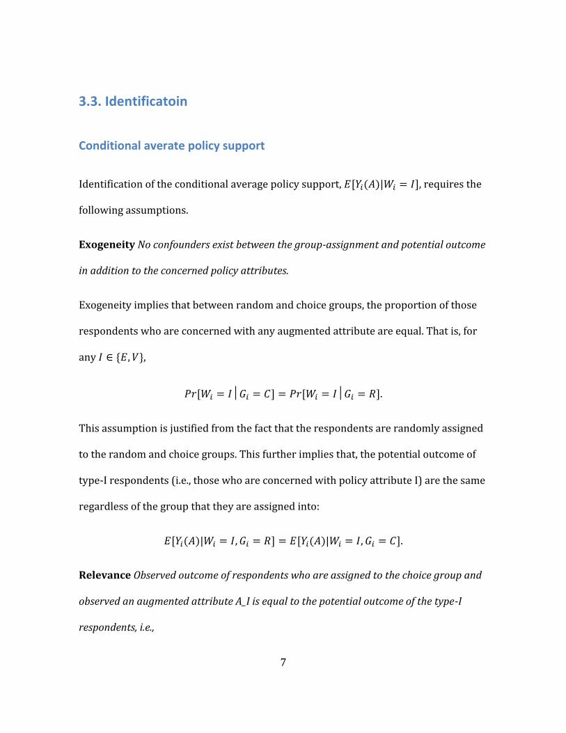
Identification of the conditional average policy support, 𝐸[𝑌𝑖(𝐴)|𝑊𝑖 = 𝐼], requires the

following assumptions.

Exogeneity No confounders exist between the group-assignment and potential outcome

in addition to the concerned policy attributes.

Exogeneity implies that between random and choice groups, the proportion of those

respondents who are concerned with any augmented attribute are equal. That is, for

any 𝐼 ∈ {𝐸, 𝑉},

𝑃𝑟[𝑊𝑖 = 𝐼│𝐺𝑖 = 𝐶] = 𝑃𝑟[𝑊𝑖 = 𝐼│𝐺𝑖 = 𝑅].

This assumption is justified from the fact that the respondents are randomly assigned

to the random and choice groups. This further implies that, the potential outcome of

type-I respondents (i.e., those who are concerned with policy attribute I) are the same

regardless of the group that they are assigned into:

𝐸[𝑌𝑖(𝐴)|𝑊𝑖 = 𝐼, 𝐺𝑖 = 𝑅] = 𝐸[𝑌𝑖(𝐴)|𝑊𝑖 = 𝐼, 𝐺𝑖 = 𝐶].

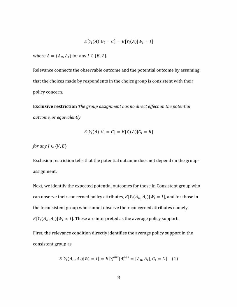
Relevance Observed outcome of respondents who are assigned to the choice group and

observed an augmented attribute A_I is equal to the potential outcome of the type-I

respondents, i.e.,

8

𝐸[𝑌𝑖(𝐴)|𝐺𝑖 = 𝐶] = 𝐸[𝑌𝑖(𝐴)|𝑊𝑖 = 𝐼]

where 𝐴 = (𝐴𝐵, 𝐴𝐼) for any 𝐼 ∈ {𝐸, 𝑉}.

Relevance connects the observable outcome and the potential outcome by assuming

that the choices made by respondents in the choice group is consistent with their

policy concern.

Exclusive restriction The group assignment has no direct effect on the potential

outcome, or equivalently

𝐸[𝑌𝑖(𝐴)|𝐺𝑖 = 𝐶] = 𝐸[𝑌𝑖(𝐴)|𝐺𝑖 = 𝑅]

for any 𝐼 ∈ {𝑉, 𝐸}.

Exclusion restriction tells that the potential outcome does not depend on the group-

assignment.

Next, we identify the expected potential outcomes for those in Consistent group who

can observe their concerned policy attributes, 𝐸[𝑌𝑖(𝐴𝐵, 𝐴𝐼)|𝑊𝑖 = 𝐼], and for those in

the Inconsistent group who cannot observe their concerned attributes namely,

𝐸[𝑌𝑖(𝐴𝐵, 𝐴𝐼)|𝑊𝑖 ≠ 𝐼]. These are interpreted as the average policy support.

First, the relevance condition directly identifies the average policy support in the

consistent group as

𝐸[𝑌𝑖(𝐴𝐵, 𝐴𝐼)|𝑊𝑖 = 𝐼] = 𝐸[𝑌𝑖𝑜𝑏𝑠|𝐴𝑖

𝑜𝑏𝑠 = {𝐴𝐵, 𝐴𝐼}, 𝐺𝑖 = 𝐶] (1)

9

for each 𝐼 ∈ {𝑉, 𝐸}, where the superscript obs indicates the observed variables. The

equation says that the observed outcomes in the choice group allows us to identify an

average support of each type of respondents.

Second is to identify the average support in the inconsistent group. The Exogeneity

and Exclusion restriction allows us to interpret the average choice support in the

randomized group as the weighted average of policy support in the consistent and

inconsistent groups;

𝐸[𝑌𝑖𝑜𝑏𝑠|𝐴𝑖

𝑜𝑏𝑠 = {𝐴𝐵, 𝐴𝐼}, 𝐺𝑖 = 𝑅] = 𝐸[𝑌𝑖(𝐴𝐵, 𝐴𝐼)] ≡ Pr[𝑊𝑖 = 𝐼] × 𝐸[𝑌𝑖(𝐴𝐵, 𝐴𝐼)|𝑊𝑖 = 𝐼]

+Pr[𝑊𝑖 ≠ 𝐼] × 𝐸[𝑌𝑖(𝐴𝐵, 𝐴𝐼)|𝑊𝑖 ≠ 𝐼] (2).

for any 𝐼 ∈ {𝑉, 𝐸}. Here, the second equality yields that

𝐸[𝑌𝑖(𝐴𝐵, 𝐴𝐼)|𝑊𝑖 ≠ 𝐼] =1

Pr[𝑊𝑖 ≠ 𝐼]𝐸[𝑌𝑖(𝐴𝐵, 𝐴𝐼)]

−Pr[𝑊𝑖 = 𝐼]

Pr[𝑊𝑖 ≠ 𝐼]𝐸[𝑌𝑖(𝐴𝐵, 𝐴𝐼)|𝑊𝑖 = 𝐼] (3)

for any 𝐼 ∈ {𝑉, 𝐸}. The average policy support in the inconsistent group can be then

rewritten by the average policy support in the randomized and the consistent group.

Finally, combining equations (1) to (3) yields the identified average support in the

inconsistent group as

𝐸[𝑌𝑖(𝐴𝐵, 𝐴𝐼)|𝑊𝑖 ≠ 𝐼] =1

Pr[𝑊𝑖 ≠ 𝐼]𝐸[𝑌𝑖

𝑜𝑏𝑠|𝐴𝑖𝑜𝑏𝑠 = {𝐴𝐵 , 𝐴𝐼}, 𝐺𝑖 = 𝑅]

10

−Pr[𝑊𝑖 = 𝐼]

Pr[𝑊𝑖 ≠ 𝐼]𝐸[𝑌𝑖

𝑜𝑏𝑠|𝐴𝑖𝑜𝑏𝑠 = {𝐴𝐵, 𝐴𝐼}, 𝐺𝑖 = 𝐶]. (4)

AMCE

The average marginal component effect, AMCE (Hainmueller, Hopkins, & Yamamoto,

2014) is useful to understand the structure of the average policy support. Because

attribute levels are randomized, AMCEs are also simply identified.

Without loss of generality, let us suppose 𝐴 = {𝐴𝐵, 𝐴𝐼}. First, equations (1) and (2)

yield that the AMCE of attribute 𝑙 for consistent group is that

𝜋𝑙(𝑎1, 𝑎0|𝑊𝑖 = 𝐼) ≡ 𝐸[𝑌𝑖(𝑎1, 𝐴−𝑙) − 𝑌𝑖(𝑎0, 𝐴−𝑙)|𝑊𝑖 = 𝐼]

= 𝐸[𝑌𝑖𝑜𝑏𝑠|𝐴𝑖

𝑜𝑏𝑠 = {𝑎1, 𝐴−𝑙}, 𝐺𝑖 = 𝐶] − 𝐸[𝑌𝑖𝑜𝑏𝑠|𝐴𝑖

𝑜𝑏𝑠 = {𝑎0, 𝐴−𝑙}, 𝐺𝑖 = 𝐶],

where 𝑎𝑖 for 𝑖 ∈ {0,1} is the level of the 𝑙th attribute, 𝐴𝑙 . AMCE of changing attribute 𝑙’s

level from a0 to a1 for for both groups in general is

𝜋𝑙(𝑎1, 𝑎0) ≡ 𝐸[𝑌𝑖(𝑎1, 𝐴−𝑙) − 𝑌𝑖(𝑎0, 𝐴−𝑙)]

= 𝐸[𝑌𝑖𝑜𝑏𝑠|𝐴𝑖

𝑜𝑏𝑠 = {𝑎1, 𝐴−𝑙}, 𝐺𝑖 = 𝑅] − 𝐸[𝑌𝑖𝑜𝑏𝑠|𝐴𝑖

𝑜𝑏𝑠 = {𝑎0, 𝐴−𝑙}, 𝐺𝑖 = 𝑅].

These together with equation (3), finally give the AMCE in the inconsistent group as

𝜋𝑙(𝑎1, 𝑎0|𝑊𝑖 ≠ 𝐼) ≡ 𝐸[𝑌𝑖(𝑎1, 𝐴−𝑙)|𝑊𝑖 ≠ 𝐼] − 𝐸[𝑌𝑖(𝑎0, 𝐴−𝑙)|𝑊𝑖 ≠ 𝐼]

=1

Pr[𝑊𝑖 ≠ 𝐼]𝜋𝑙(𝑎1, 𝑎0) −

Pr[𝑊𝑖 = 𝐼]

Pr[𝑊𝑖 ≠ 𝐼]𝜋𝑙(𝑎1, 𝑎0|𝑊𝑖 = 𝐼).

11

Difference-in-means

The difference of policy supports between consistent and inconsistent groups is

defined as

𝐸[𝑌𝑖(𝐴𝐵, 𝐴𝐼)|𝑊𝑖 = 𝐼] − 𝐸[𝑌𝑖(𝐴𝐵, 𝐴𝐼)|𝑊𝑖 ≠ 𝐼],

which can be identified by combining equations (1) and (4) as

𝐸[𝑌𝑖(𝐴𝐵, 𝐴𝐼)|𝑊𝑖 = 𝐼] − 𝐸[𝑌𝑖(𝐴𝐵, 𝐴𝐼)|𝑊𝑖 ≠ 𝐼] = 𝐸[𝑌𝑖𝑜𝑏𝑠|𝐴𝑖

𝑜𝑏𝑠 = 𝐴𝐵, 𝐴𝐼 , 𝐺𝑖 = 𝐶]

−1

𝑃𝑟[𝑊𝑖 ≠ 𝐼]𝐸[𝑌𝑖

𝑜𝑏𝑠|𝐴𝑖𝑜𝑏𝑠 = 𝐴𝐵 , 𝐴𝐼 , 𝐺𝑖 = 𝑅]

+𝑃𝑟[𝑊𝑖 = 𝐼]

𝑃𝑟[𝑊𝑖 ≠ 𝐼]𝐸[𝑌𝑖

𝑜𝑏𝑠|𝐴𝑖𝑜𝑏𝑠 = 𝐴𝐵 , 𝐴𝐼 , 𝐺𝑖 = 𝐶]

=(𝐸[𝑌𝑖

𝑜𝑏𝑠|𝐴𝑖𝑜𝑏𝑠 = {𝐴𝐵, 𝐴𝐼}, 𝐺𝑖 = 𝐶] − 𝐸[𝑌𝑖

𝑜𝑏𝑠|𝐴𝑖𝑜𝑏𝑠 = {𝐴𝐵, 𝐴𝐼}, 𝐺𝑖 = 𝑅])

(𝑃𝑟[𝑊𝑖 ≠ 𝐼]).

Note that this expression allows us to apply the machine learning technique to detect

any relevant heterogeneity in causal effects between consistent and inconsistent

group with respect to the set of attributes to be observed. Specifically, the causal

forest is applied to estimate the numerator, i.e., 𝐸[𝑌𝑖𝑜𝑏𝑠|𝐴𝑖

𝑜𝑏𝑠 = {𝐴𝐵, 𝐴𝐼}, 𝐺𝑖 = 𝐶] −

𝐸[𝑌𝑖𝑜𝑏𝑠|𝐴𝑖

𝑜𝑏𝑠 = {𝐴𝐵, 𝐴𝐼}, 𝐺𝑖 = 𝑅].

12

4. Estimation.

This section reports the estimation results especially the AMCE.

4.1. AMCE.

The AMCE in the controlled group are firstly shown. The results capture the policy

preference without additional treatment.

Fig 1. Baseline AMCEs.

13

The figure shows that respondents tend to prefer reforms (1) more burden for the

rich elders, (2) allowing mixed elderly care, (3) expanding the contents of care service,

while do not prefer (1) increasing payment age of public pension, (2) more burden for

the working age, and (3) increasing self-payment.

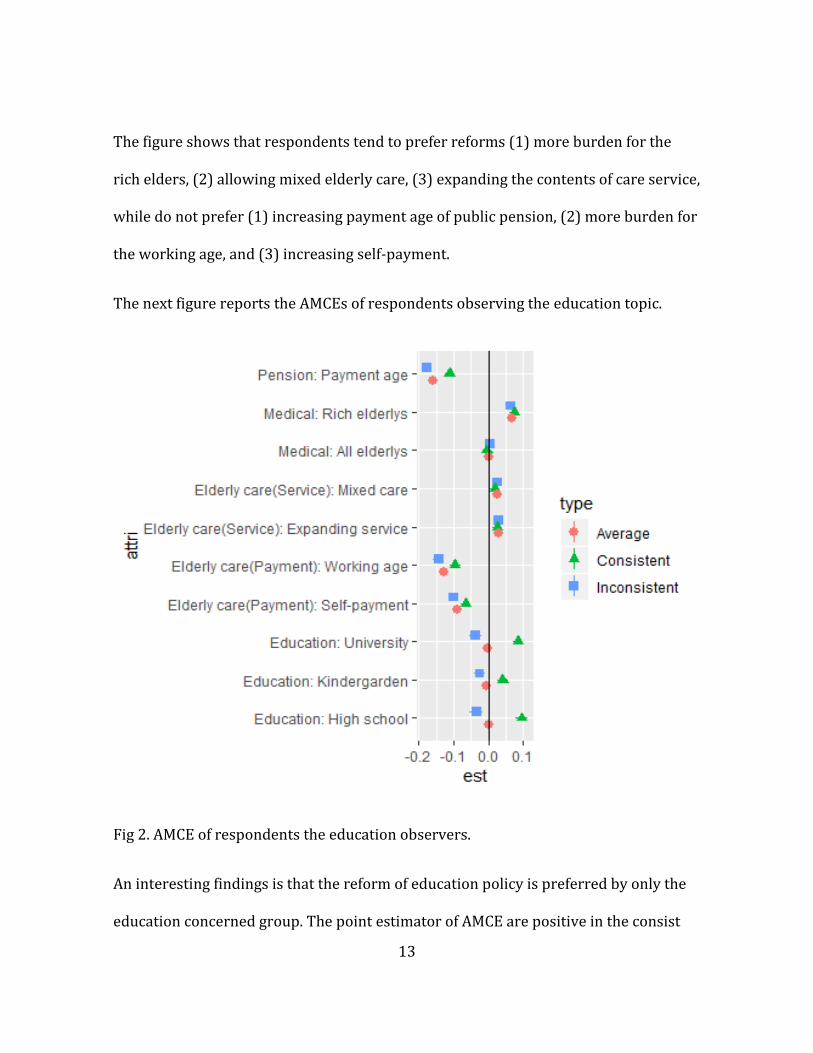
The next figure reports the AMCEs of respondents observing the education topic.

Fig 2. AMCE of respondents the education observers.

An interesting findings is that the reform of education policy is preferred by only the

education concerned group. The point estimator of AMCE are positive in the consist

14

group while negative in the inconsistent group, which implies that the AMCE of those

reform is quit small and statistically insignificant, and the inconsistent group do not

then prefer.

Among the education reform, the scholarship for undergraduates and high school is

more preferred than the kindergarten.

The preference for basic attributes are qualitatively same with the baseline results,

but some quantitative heterogeneous is found. The negative impacts of pension and

elderly care reform are weaker in the consistent group than education concerned

groups in the inconsistent group.

15

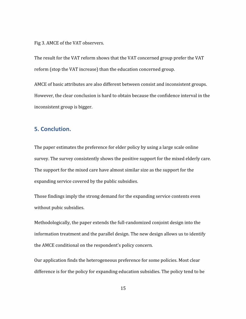
Fig 3. AMCE of the VAT observers.

The result for the VAT reform shows that the VAT concerned group prefer the VAT

reform (stop the VAT increase) than the education concerned group.

AMCE of basic attributes are also different between consist and inconsistent groups.

However, the clear conclusion is hard to obtain because the confidence interval in the

inconsistent group is bigger.

5. Conclution.

The paper estimates the preference for elder policy by using a large scale online

survey. The survey consistently shows the positive support for the mixed elderly care.

The support for the mixed care have almost similar size as the support for the

expanding service covered by the public subsidies.

Those findings imply the strong demand for the expanding service contents even

without pubic subsidies.

Methodologically, the paper extends the full-randomized conjoint design into the

information treatment and the parallel design. The new design allows us to identify

the AMCE conditional on the respondent’s policy concern.

Our application finds the heterogeneous preference for some policies. Most clear

difference is for the policy for expanding education subsidies. The policy tend to be

16

supported by respondents concerning the education policy, while not supported by

the VAT concerned respondents. Meanwhile, the support for the mixed care is not

significantly different.

17

Reference

• Athey, S., & Wager, S. (2019). Estimating Treatment Effects with Causal Forests:

An Application. arXiv preprint arXiv:1902.07409.

• Athey, S., Tibshirani, J., & Wager, S. (2019). Generalized random forests. The

Annals of Statistics, 47(2), 1148-1178.

• Bansak, K., Hainmueller, J., Hopkins, D. J., & Yamamoto, T. (2017). Beyond the

breaking point? Survey satisficing in conjoint experiments. Political Science

Research and Methods, 1-19.

• Bansak, K., Hainmueller, J., Hopkins, D. J., & Yamamoto, T. (2018). The number of

choice tasks and survey satisficing in conjoint experiments. Political Analysis,

26(1), 112-119.

• Bechtel, M. M., & Scheve, K. F. (2013). Mass support for global climate agreements

depends on institutional design. Proceedings of the National Academy of

Sciences, 110(34), 13763-13768.

• Chernozhukov, V., Demirer, M., Duflo, E., & Fernandez-Val, I. (2018). Generic

machine learning inference on heterogenous treatment effects in randomized

experiments (No. w24678). National Bureau of Economic Research.

18

• Hainmueller, J., Hopkins, D. J., & Yamamoto, T. (2014). Causal inference in

conjoint analysis: Understanding multidimensional choices via stated preference

experiments. Political Analysis, 22(1), 1-30.

• Hainmueller, J., Hangartner, D., & Yamamoto, T. (2015). Validating vignette and

conjoint survey experiments against real-world behavior. Proceedings of the

National Academy of Sciences, 112(8), 2395-2400.

• Horiuchi, Y., Smith, D. M., & Yamamoto, T. (2018). Measuring voters’

multidimensional policy preferences with conjoint analysis: Application to

Japan’s 2014 election. Political Analysis, 26(2), 190-209.

• Wager, S., & Athey, S. (2018). Estimation and inference of heterogeneous

treatment effects using random forests. Journal of the American Statistical

Association, 113(523), 1228-1242.

19

Appendix.

Attributes estimate conf.low conf.high

Constant 0.610 0.604 0.616

Elderly care(Payment): Self-payment -0.095 -0.100 -0.090

Elderly care(Payment): Working age -0.137 -0.142 -0.132

Elderly care(Service): Mixed care 0.028 0.023 0.033

Elderly care(Service): Expanding service 0.035 0.030 0.040

Medical: All elderlys -0.002 -0.007 0.004

Medical: Rich elderlys 0.066 0.061 0.071

Pension: Payment age -0.149 -0.154 -0.144

Table A-1. AMCE wihtout additional attributes.

20

Type Attribute estimate conf.low conf.high

Average Elderly care(Payment): Self-payment -0.095 -0.105 -0.085

Average Elderly care(Payment): Working age -0.131 -0.141 -0.121

Average Elderly care(Service): Mixed care 0.009 0.000 0.019

Average Elderly care(Service): Expanding

service

0.032 0.022 0.042

Average Medical: All elderlys -0.001 -0.010 0.008

Average Medical: Rich elderlys 0.048 0.038 0.058

Average Pension: Payment age -0.121 -0.129 -0.112

Average VAT: Still 8% 0.137 0.126 0.148

Average VAT: delay 0.064 0.053 0.074

Type Attribute estimate conf.low conf.high

Consistent Elderly care(Payment): Self-payment -0.092 -0.100 -0.083

Consistent Elderly care(Payment): Working age -0.128 -0.137 -0.120

Consistent Elderly care(Service): Mixed care 0.022 0.014 0.030

Consistent Elderly care(Service): Expanding

service

0.029 0.021 0.037

Consistent Medical: All elderlys -0.013 -0.021 -0.005

Consistent Medical: Rich elderlys 0.049 0.040 0.057

21

Consistent Pension: Payment age -0.132 -0.139 -0.125

Consistent VAT: Still 8% 0.178 0.168 0.188

Consistent VAT: delay 0.089 0.081 0.097

Type Attribute estimate conf.low conf.high

Inconsistent Elderly care(Payment): Self-payment -0.104 -0.147 -0.061

Inconsistent Elderly care(Payment): Working age -0.138 -0.180 -0.096

Inconsistent Elderly care(Service): Mixed care -0.024 -0.063 0.016

Inconsistent Elderly care(Service): Expanding

service

0.040 -0.001 0.081

Inconsistent Medical: All elderlys 0.031 -0.008 0.070

Inconsistent Medical: Rich elderlys 0.048 0.005 0.090

Inconsistent Pension: Payment age -0.091 -0.124 -0.058

Inconsistent VAT: Still 8% 0.031 -0.016 0.077

Inconsistent VAT: delay 0.000 -0.043 0.042

Table A-2. AMCE of education observars.

22

Type Attribute estimate conf.low conf.high

Average Elderly care(Payment): Self-payment -0.095 -0.105 -0.085

Average Elderly care(Payment): Working age -0.131 -0.141 -0.121

Average Elderly care(Service): Mixed care 0.009 0.000 0.019

Average Elderly care(Service): Expanding

service

0.032 0.022 0.042

Average Medical: All elderlys -0.001 -0.010 0.008

Average Medical: Rich elderlys 0.048 0.038 0.058

Average Pension: Payment age -0.121 -0.129 -0.112

Average VAT: Still 8% 0.137 0.126 0.148

Average VAT: delay 0.064 0.053 0.074

Type Attribute estimate conf.low conf.high

Consistent Elderly care(Payment): Self-payment -0.092 -0.100 -0.083

Consistent Elderly care(Payment): Working age -0.128 -0.137 -0.120

Consistent Elderly care(Service): Mixed care 0.022 0.014 0.030

Consistent Elderly care(Service): Expanding

service

0.029 0.021 0.037

Consistent Medical: All elderlys -0.013 -0.021 -0.005

Consistent Medical: Rich elderlys 0.049 0.040 0.057

23

Consistent Pension: Payment age -0.132 -0.139 -0.125

Consistent VAT: Still 8% 0.178 0.168 0.188

Consistent VAT: delay 0.089 0.081 0.097

Type Attribute estimate conf.low conf.high

Inconsistent Elderly care(Payment): Self-payment -0.104 -0.147 -0.061

Inconsistent Elderly care(Payment): Working age -0.138 -0.180 -0.096

Inconsistent Elderly care(Service): Mixed care -0.024 -0.063 0.016

Inconsistent Elderly care(Service): Expanding

service

0.040 -0.001 0.081

Inconsistent Medical: All elderlys 0.031 -0.008 0.070

Inconsistent Medical: Rich elderlys 0.048 0.005 0.090

Inconsistent Pension: Payment age -0.091 -0.124 -0.058

Inconsistent VAT: Still 8% 0.031 -0.016 0.077

Inconsistent VAT: delay 0.000 -0.043 0.042

Table A-3. AMCE of VAT observars.