preface - informationsstelle edelstahl rostfrei this publication is the main outcome of the rfcs...

1

Preface

This publication is the main outcome of the RFCS funded project “Innovative stainless steel applications in transport vehicles” (INSAPTRANS: contract RFS2-CT-2007-00025). The main objective of the project is to disseminate the technical knowledge and application experience resulting from two recently finished ECSC/RFCS research projects, namely “Stainless steels in bus constructions” (STAINLESS STEEL BUS: contract 7210-PR-176) and “Development of lightweight train and metro cars by using ultra high strength stainless steels” (DOLTRAC: contract 7210-PR-363). The primary tool in the dissemination task is this handbook on advanced, lightweight stainless steel structures in ground-transport vehicles. It summarises the vast amount of result data generated and reported in these research projects. Following the printed version, this publication will also be made available in electronic format through Euro Inox.

The dissemination function of this handbook is supported by a series of six regional seminars across the European Union. A workshop to review the seminar feedback and establish networking actions among the European industrial, research and academic players on the field will follow the seminars. The workshop’s aim is also to stimulate future R&D initiatives in the area.

The main objective of this handbook is to give the designer a good overview of the possibilities modern stainless steels have to offer in the transport-vehicle industry. It gives guidelines for the application of safe, lightweight stainless steel structures in ground-transport applications and demonstrates their full potential. The handbook covers all aspects relevant to the realising of such structures, including materials, joining, forming, mechanical testing, crash behaviour, corrosion, product life-cycle cost and environmental impact.

For more detailed result data, the reader is advised to consult the actual final reports of the projects:

• Kyröläinen, A., Sánchez, R., Santacreu, P.-O., Picozzin, V. and Gales, A. 2003. Stainless steels in bus contructions. Luxembourg, Office for Official Publications of the European Communities, Technical Steel Research, Special and Alloy Steels, Report EUR 20884, ISBN 92-894-6635-9. 457 p.

• Gales, A., Sirén, M., Säynäjäkangas, J., Akdut, N., van Hoecke, D. and Sánchez, R. 2007. Development of lightweight train and metro cars by using ultra high strength stainless steels. Office for Official Publications of the European Communities, Technical Steel Research, Report EUR 22837, ISBN 92-79-05526-3. 266 p.

2

For obvious reasons, these two final reports are referred to frequently in this handbook. To avoid complicated cross-references in the text, they are referred to simply by the project acronym and, where appropriate, the page number – e.g. (BUS p. 99) or (DOLTRAC p. 88).

The European stainless steel industry and its organisations and relevant research institutions are continuing their efforts to develop the use of stainless steel in the transport sector. The co-funding by the European Union of STAINLESS STEEL BUS, DOLTRAC and INSAPTRANS has helped deepen insight into the specific needs of both bus and rolling-stock manufacturers and public-transport operators. Interested designers and manufacturers are encouraged to contact the participating partners of these projects, now and in the future. The stainless steel industry will be keen to discuss new market requirements, against the background of novel solutions in terms of materials, design and fabrication. The research organisations involved in R&D related to stainless steel are equally keen to participate in this work, together with the stainless steel industry.

3

Contents

Preface ............................................................................................................................... 1

1. Introduction: stainless steels in transport vehicles ....................................................... 7

1.1 Rail applications history ..................................................................................... 7

1.2 Current rail applications ................................................................................... 10

1.3 Bus and coach applications .............................................................................. 14

1.4 Future potential ................................................................................................. 16

2. Materials .................................................................................................................... 19

2.1 Grades ............................................................................................................... 20

2.2 Delivery conditions .......................................................................................... 24

2.3 Mechanical behaviour and design values ......................................................... 25

2.3.1 Tensile properties of the project materials ........................................... 26

2.3.2 Design values and physical properties of stainless steels .................... 26

2.4 Corrosion properties ......................................................................................... 31

2.4.1 Atmospheric corrosion ......................................................................... 32

2.4.2 De-icing and dust-control chemicals .................................................... 34

2.4.3 Corrosion resistance evaluation ........................................................... 35

2.4.4 Corrosion test results ............................................................................ 37

2.4.5 Corrosion test summary ....................................................................... 44

2.5 Stainless steel high-temperature mechanical properties: fire resistance .......... 46

2.6 Selection of materials ....................................................................................... 49

2.6.1 Structural applications .......................................................................... 49

2.6.2 Forming applications ............................................................................ 51

2.6.3 Summary .............................................................................................. 53

3. Lightweight structures and design ............................................................................. 55

3.1. Stainless hollow-section structures .................................................................. 55

3.1.1. Manufacture of hollow sections ....................................................................... 55

3.1.2. Structural design aspects for hollow-section joints .......................................... 56

3.2. Sandwich panel structures ................................................................................ 62

3.2.1 Design principles of sandwich panels .................................................. 65

3.2.2 Panel cross-section ............................................................................... 66

3.2.3 Elastic response .................................................................................... 66

3.2.4 Strength and deflection criteria ............................................................ 67

3.2.5 Structural optimisation ......................................................................... 68

3.2.6 Design tools .......................................................................................... 69

3.2.7 Special issues in all-steel sandwich panel design ................................ 70

4

4. Manufacturing issues in lightweight structures ........................................................... 73

4.1 Bending of high strength stainless steel sheets................................................. 73

4.1.1 Verification of minimum sheet bending radius .................................... 74

4.1.2 Determination of sheet springback behaviour ...................................... 75

4.1.3 Guidelines for bending ultra high-strength stainless steel ................... 77

4.2 Tube bending .................................................................................................... 77

4.2.1 Types of mechanical tube-bending processes ...................................... 77

4.2.2 Springback model ................................................................................. 78

4.2.3 Rectangular tube-bending results ......................................................... 79

4.2.4 Design guidance for three-roll tube bending ........................................ 81

4.3 Welding and joining ......................................................................................... 82

4.3.1 Arc-based welding processes ............................................................... 82

4.3.2 Laser-based welding processes ............................................................ 85

4.3.3 Resistance welding ............................................................................... 86

4.3.4 Adhesive bonding ................................................................................. 87

5. Properties of lightweight structures ........................................................................... 89

5.1. Welded joint properties .................................................................................... 89

5.1.1 Static strength ....................................................................................... 89

5.1.2 Fatigue and corrosion fatigue strength ................................................. 94

5.2 Sandwich panel mechanical properties ............................................................ 96

5.2.1 Four-point bend testing of full-size panels ........................................... 97

5.2.2 Three-point bend testing of panel sections ........................................... 98

5.2.3 Summary and conclusions .................................................................. 100

5.3 Lightweight structure crash properties ........................................................... 102

5.3.1 Axial impact tests ............................................................................... 102

5.3.2 Side impact tests ................................................................................. 102

5.3.3 Tubular frame crash tests ................................................................... 103

5.3.4 Panel compression and crash testing .................................................. 105

6. Life cycle issues ....................................................................................................... 109

6.1. Effect of vehicle weight on life cycle cost ..................................................... 109

6.2. Environmental effects of bus-frame materials ............................................... 111

6.3. Life cycle cost evaluation of bus-frame materials .......................................... 112

6.4. Summary ........................................................................................................ 115

Acknowledgements ....................................................................................................... 117

References ..................................................................................................................... 118

5

List of symbols

Mechanical properties A(50) Elongation to fracture (gauge length) E Elastic modulus fu Ultimate tensile strength (of a material) ≈ Rm fy Yield strength (of a material) ≈ Rp0.2 KV Fracture energy Rm Tensile strength ≈ fu Rp0.2 0.2 % proof strength ≈ fy

Physical properties α Coefficient of thermal expansion c Specific heat capacity λ Thermal conductivity ρ Resistivity RT Room temperature

Structures CHS Circular hollow section RHS Rectangular hollow section SHS Square hollow section g Gap between brace members (in hollow section structures) θ Joint angle (in hollow section structures) t Thickness

Welding and joining ADB Adhesive bonding GMAW Gas metal arc welding = MIG/MAG GTAW Gas tungsten arc welding = TIG HF High frequency induction welding LBW Laser beam welding MAG Metal active gas welding = GMAW MIG Metal inert gas welding = GMAW PAW Plasma arc welding PPAW Powder plasma arc welding RSW Resistance spot welding TIG Tungsten inert gas welding = GTAW WB Weld bonding: combination of ADB and RSW

7

1. Introduction: stainless steels in transport vehicles

The use of stainless steel in ground transport is by no means new: its track record goes back nearly three quarters of a century. In the case of railway coaches, it was durability and ease-of-maintenance considerations, especially, that tipped the balance towards stainless steel. With design lives of often more than 40 years, rolling stock is an application for which it is worthwhile considering intrinsically corrosion-resistant materials.

Buses and coaches have a service life of 20 years and more. For coatings on less corrosion-resistant materials, such a long time span is difficult to survive without major maintenance and repair. Condensation and the influence of de-icing salt can make corrosion protection a challenge. For this reason, stainless steel has also been used successfully not only for the skin but also the structure of buses and coaches.

Over the years, rail and bus technology has developed – and so has stainless steel. The refinement of metallurgical processes has further improved the uniformity and corrosion-resistance of proven chromium-nickel stainless steels. The range of mechanical treatments to further enhance their mechanical properties has been extended. New grades have been developed, including chromium-manganese types, which combine cost reduction with high mechanical strength. Ferritic stainless steels have given rail and bus manufacturers new and particularly cost-effective options, especially for the outer skin of vehicles when customers require painting for reasons of corporate design. It is the purpose of the present publication to give a research-based overview of the new potential that has emerged over the last few years.

1.1 Rail applications history

Invented in the early 20th century, stainless steels were soon applied to the rail industry. The 1930’s brought widespread use of stainless steel for rail coach bodies. Weight reduction became a priority and laid the ground for levels of speed and comfort that had not been experienced before. Especially in North America, stainless steel became the preferred material for rail coaches.

Although stainless steel is neither the lightest of materials nor the least expensive, both manufacturers and operators soon discovered that its outstanding long-term corrosion resistance provided maintenance and cost advantages. The fact that painting became redundant made stainless steel even more attractive. However, it was also a marketing issue. Long-distance rail travel was positioned as a modern, technologically advanced option for the demanding customer and stainless steel was an icon for this idea.

8

Figure 1. Rear view of El Capitan. Figure 2. Observation end of the Pioneeer

Colorado, 1938 (Denver Public Library Zephyr (Wikipeda 2007a).

2007).

Much of the enthusiasm for stainless steel has been maintained over the decades, both for technical reasons and as a matter of aesthetic preference. Stainless steel is equally present in metro, commuter and long distance-trains to the present day.

In Europe, the history of stainless steel in rail transport did not start until after World War II. Inspired by the North American experience, several national railway companies welcomed stainless steel solutions suggested by rolling-stock manufacturers. Stainless steel succeeded at both ends of the scale, both in commuter trains and luxury long-distance trains.

As a predecessor of today’s high-speed European trans-national rail connections, the “Trans Europ Express” (TEE) was the epitome of speed and comfort in the 50s and 60s. On the Paris–Brussels–Amsterdam (TEE PBA) line, stainless steel rail coaches were introduced in 1962. This service was only suspended in 1996, with the arrival of today’s high-speed trains.

Figure 3. The Paris-Brussels-Amsterdam

Trans Europ Express service (TEE PBA)

started in 1962 (Trains en voyage 2007).

9

In contrast to express-train carriages, many of the metro trains developed in the late 50s and early 60s for commuter service are still in service. However, their refurbishment often involves partial or total painting, to make their appearance consistent with the corporate-design requirements of the rail operators. One of these is the “RIO” and “RIB” series of commuter trains in France. The acronyms stand for rame inox omnibus and rame inox banlieue respectively – i.e. stainless steel commuter train. Figure 4. French RIO series commuter Figure 5. Fleet of RIB trains near Paris

train (Rinaldi 2007). (Pauly 2007).

In Germany, a new type of railway carriage, called Silberling (“silverling”) by railway enthusiasts, marked a new development in commuter service. Prototypes became available in 1958. With a weight of 28.5 t empty and a service weight of 31-40 t, depending on equipment, it was a particularly lightweight model for its time. Mass production started in 1961 and continued until 1980. Some have survived in regional service after more than 45 years of service, however they are now in the corporate-design colours of the railway operator.

Figure 6. German “Silberling” rail coach

prior to refurbishment and painting

(Wikipedia 2007b).

10

In Japan and the Asia-Pacific areas, stainless steel has continued to be used throughout the 1970s to the present day.

Figure 7. Double-decker interurban rail

coaches introduced in New South Wales

(Australia) in 1970 (Wikipedia 2007c).

1.2 Current rail applications

In many parts of the world, notably in North America, early experiences with stainless steel have influenced the preference of railway operators, rail-coach manufacturers and passengers alike. Unpainted, profiled stainless steel panels continue to be the “normal” material.

Figure 8. Metro, Chicago (Pauly 2007).

Figure 9. Regional train, Baltimore Figure 10. Double-decker train, Chicago

(Pauly 2007). (Pauly 2007).

11

Besides aesthetic criteria, safety considerations are increasingly taken into account. Although serious collisions are very infrequent these days, higher operating speeds increase the likelihood of injury when they do occur. Many rail companies have therefore chosen to construct carriages from austenitic stainless steel, in preference to alternative materials such as carbon steel and aluminium alloys. This choice carries a unique safety-related benefit, attributable first and foremost to the high energy-absorption made possible by the unique work-hardening properties of austenitic stainless steels. If the assembly is properly designed, stainless steel tubular sections will fail in compression – not in buckling. The inherent material strength increases as the speed and intensity of the deformation increases, thus maximising energy absorption.

Figure 11. The crush behaviour of stainless steel circular hollow section maximises energy absorption in the event of a collision (Euro Inox 2006a).

In India, for instance, there is an ongoing programme to replace the present COR-TEN® steel long-distance coaches with lightweight all-stainless steel coaches. These will be in unpainted stainless steel grade AISI 301LN (EN 1.4318) – a material with particularly marked work-hardening properties which has already been successfully used in Indian metro trains. Two major manufacturers roll out 1,000 coaches a year, each coach using approximately 6.5 metric tons of stainless steel. Figure 12. Stainless steel long-distance

coach, India (Gopal 2007a).

12

Figure 13. Delhi metro coach (Gopal 2007b).

In Europe, the development of stainless steel has taken a distinctly different course from that in North America, Asia and other parts of the world. Although unpainted austenitic stainless steel is present in a number of metro systems (Lisbon, for example), painted surfaces are generally preferred.

Figure 14. Stainless steel metro trains were

introduced to Lisbon in the early 90s

(Bombardier 2007).

The reason is often non-technical. Rail operators have stringent corporate-design requirements, which typically involve a colour code to differentiate different types of train. The fact that there is no need for painting is therefore no longer perceived as an advantage. A case in point is the Swedish X-2000 high-speed tilting train, the skin of which was originally in unpainted austenitic stainless steel. Launched in 1990, this train was, however, repainted in grey as of 2005.

Figure 15. X-2000 high-speed tilting train,

Sweden (Wikipedia 2007d).

13

Nevertheless, the superior corrosion resistance of stainless steel remains a valid argument in favour of the material. Ferritic stainless steels have turned out to be a preferred solution. Since they are not alloyed with nickel, ferritics are significantly lower in initial cost than austenitic grades. As painting is a corporate-design requirement, lower-alloyed stainless steels in the 12 % Cr range qualify for the application. These steels are therefore present in today’s rolling stock, although less visibly.

Figure 16. Two-car unit with a stainless steel body, Balmaseda, Spain

(Feve 2007).

Figure 17. Trams in painted ferritic stainless steel, Hanover (Germany) (ThyssenKrupp

Stainless 2007).

14

1.3 Bus and coach applications

As in the case of railway carriages, preference for stainless steel was to a large extent an American phenomenon. The image of long-distance bus connections has been associated with the bright and shiny appearance of stainless steel buses since the 1940’s. This tradition continues to the present day.

Figure 18. Stainless steel bus, Mexico (Pauly

2007).

In Europe, studies focussing on the weld integrity of stainless steels in bus and coach applications have demonstrated the technical superiority of stainless steel. Safety aspects have been studied, based on fracture mechanics and impact-toughness testing. The fatigue resistance of welded rectangular hollow section (RHS) profiles was evaluated according to the Eurocode 3 (1992) fatigue standard. Corrosion resistance was studied by salt-spray-chamber tests in a de-icing salt atmosphere and by field testing for 3 years under an urban bus. The mechanical tests show that in these applications austenitic stainless steel EN 1.4310 (AISI 301) is a superior material and that low-carbon 12 % Cr alloyed stainless steel EN 1.4003 is also competitive. According to life cycle cost (LCC) calculations, stainless steels are competitive compared with carbon steels or aluminium (Kyröläinen et al. 2000).

European bus manufacturers started using stainless steel in the early 1990s. Development started specifically in Scandinavia, where a cold and humid climate, often involving the use of de-icing salts, explains operators’ willingness to consider a corrosion-resistant material such as stainless steel.

Figure 19. Coach with a stainless steel body

frame and skin (Volvo Bus 2007).

15

In Central European countries such as Belgium, Germany and the Netherlands, stainless steel also became a common option.

Figure 20. Articulated bus with a skin in

ferritic stainless Steel (Van Hool 2007).

Italy, with its dense network of publicly operated inter-regional bus connections, became another centre of stainless steel use in buses and coaches. In vehicle structure, classic grades such as 1.4301 (AISI 304) have maintained a dominant position. Manufacturers particularly appreciate this material’s excellent weldability. In panelling, ferritic steels such as 1.4003 have gained ground. Comparable in initial cost to coated carbon steels, they will not suffer significant corrosion even if the paintwork gets damaged – which is hard to avoid in the rough conditions of public transport.

Figure 21. Assembly of buses with a Figure 22. Welding of a bus chassis from

stainless steel chassis and (ferritic) square hollow sections, in grade EN 1.4301

stainless steel skin (Centro Inox 2007a / (AISI 304) (Centro Inox 2007b).

De Simon 2007).

Typically, about 200 m of square hollow sections and 600 kg of stainless steel sheet go into a bus. Grade 304 (1.4301) with a 2B finish is usually used as a standard option. Polyurethane adhesives are used to attach the shell to the structure (Australian Stainless 2001). Compared with conventional designs, 700 kg in weight reduction and 15 % reduction in production time have been reported.

16

1.4 Future potential

Future prospects for stainless steel in rail and bus applications are expected to focus around two axes: the development of work-hardened stainless steel fabricated components and the greater use of ferritic grades. Ferritic stainless steel has also been tested successfully for structural applications. In this context, another aspect of innovation has been the increasing use of mechanical fasteners. This was inspired by the concept of modular design, which makes future refurbishment easier and less costly.

Figures 23 and 24. Experimental structure

and wall of a railway carriage in laser-cut

ferritic stainless steel hollow sections, using a

mechanical fastening technique (Pauly 2007).

An example of the weightsaving potential of stainless steel can be found in the U.S., where the Department of Energy is supporting an R&D project of a prototype, hybrid electric, ultra-light, stainless steel, 40-foot urban bus. This bus features a low-floor monocoque-type structure, four-wheel independent suspension (with no interior intrusion for axle clearance) and a front-frame crush zone to improve occupant safety in the event of a collision. The bus has an estimated curb weight of only 4,400 kg, which represents a mass reduction of 64 % compared to conventional buses and thus improves passenger-carrying payload and fuel economy.

Figure 25. Rear view of an ultra-light,

stainless steel, hybrid electric transit bus

being developed under a DOE/industry

partnership (Fisher 2008).

17

In addition to the weight and fuel-economy improvements, Department of Energy officials expect the bus to be 40 % less costly to build. The cost model for the prototype vehicle can be found in Figure 27 (Emmons 2006). The project shows that in the two main criteria for the development of public transport – cost reduction and a reduction of the use of fossil fuels – stainless steel can make a contribution.

Figure 26. Prototype of driver’s station Figure 27. Cost model of the

(Emmons 2006). prototype vehicle (Emmons 2006).

19

2. Materials

By definition, stainless steels are high-alloyed steels with a composition of more than 10.5 wt % chromium (Cr) and less than 1.2 wt % carbon (C). This chromium alloying gives the material superior corrosion resistance properties compared to mild (e.g. C-Mn) steels. Stainless steels are usually further divided into four main sub-categories according to their microstructure: ferritic, martensitic, austenitic and austenitic-ferritic (i.e. duplex) grades.

Ferritic stainless steels are characterised by good strength and toughness properties and by their magnetism. Furthermore, they have reasonable resistance to general corrosion and good stress-corrosion properties. Typical applications are in moderately aggressive environments (e.g. under conditions of atmospheric corrosion and in the vehicle industry, such as in bus and coach bodies).

Martensitic stainless steels show high strength and wear-resistance and are magnetic. Their strength and toughness properties can be adjusted by hardening and tempering but their resistance to general corrosion is the lowest among stainless steels. Instead, they show good resistance to cavitation corrosion, so their main application areas include ship propellers and water turbines. They are also used in tools, conveyor screws, winches and vehicle components such as brake discs.

Austenitic stainless steels are non-magnetic, work-hardenable grades that show excellent strength and toughness properties. Depending on their alloying degree – typically 17 - 24 wt % Cr and 6 - 25 wt % Ni – they have a good to excellent general-corrosion and pitting-corrosion resistance. Austenitic grades are the most widely used stainless steels and their applications range from electronics and electrical to the process industries. In the transport industry, they are commonly used for tank containers and bus or coach body structures.

Austenitic-ferritic (i.e. duplex) stainless steels combine the best properties of ferritic and austenitic grades. Their high chromium and molybdenum content results in excellent general-corrosion and pitting-corrosion resistance and the duplex microstructure – 50/50 ferrite and austenite – yields exceptionally good stress-corrosion resistance and high mechanical strength. Duplex stainless steels are particularly suitable for dynamically loaded high-strength applications such as pump and valve shafts and for process-industry equipment such as boiling tanks and wood-pulp silos. Lately, there has been some experimental use of so-called lean duplex stainless steel grades for trucks, where the high mechanical properties of the material have made it possible to minimise tare and increase payload.

20

Ferritic and austenitic grades are the most commonly used stainless steel types in transport-vehicle structural applications. Other types are mostly used in powertrain or chassis components. Our main emphasis, therefore, will be on the ferritic and austenitic grades used or on showing potential in vehicle structures, especially with regard to weight reduction and/or safety issues. Compared to austenitic steels, ferritic grades offer a price stability that is of particular importance for high-volume products and models. New leaner alloys developed in austenitic and duplex grades are responding to the price fluctuations of certain alloying elements, especially nickel, by substituting manganese and nitrogen.

2.1 Grades

Due to their outstanding mechanical and corrosion-resistance properties, stainless steels meet the technical requirements of a great number of applications, provided the right grade is selected for the particular use and proper fabrication and maintenance conditions are observed. Taking cost and environment-related aspects into account, the BUS and DOLTRAC projects referred to herein assess the suitability of the stainless steel grades described below for use in structural parts of buses, railway and metro cars, especially in terms of fabricability and in-service performance.

Stainless steels offer many alternatives for safe structures, from both service-environment (typically corrosion) and mechanical-safety viewpoints. In the BUS project, two traditional grades, austenitic 1.4301 and ferritic 1.4003, and two new types of steel, 304SP and 16-7Mn, were chosen for experiments. Grade 304SP is an austenitic stainless steel of type 18Cr-8Ni-1Mo-N (a variant of popular European grade 1.4301), optimised in terms of mechanical properties and corrosion resistance, for the needs of the transport industry. Grade 16-7Mn is an austenitic stainless steel of type 16Cr-1.5Ni-7Mn-N. Only produced in one experimental heat for use in, for example, the BUS Project, it has a composition and thus presumably properties resembling those of the more established and standardised AISI 200 series grades. Specifically, the recently introduced “European” Type-200, EN 1.4618 steel is a commercially available grade with comparable properties. Both above-mentioned steels, in the form of annealed/cold formed sheets (2H), hollow sections and formed tubes have been investigated here. The 2H condition meets the the C850 strength-class requirement (Rm ≥ 850 N/mm2) of European Standard EN 10088-2. All tubes, except for some hydroformed examples, were in non-heat-treated condition and thus had increased strength.

In 304SP, molybdenum and nitrogen alloying enhances pitting-corrosion resistance in chloride solutions and also increases strength. The idea behind 16-7Mn steel is to replace an expensive raw material (nickel) with manganese. This also increases the strength of the steel. By the same token, high manganese content makes it possible to

21

use higher nitrogen contents in austenitic stainless steel, which increases corrosion resistance in chloride solutions.

One of the most promising stainless steels for transport applications is austenitic grade 1.4318 (AISI 301LN). Cold rolled, high-strength 1.4318 sheets or hollow sections can make possible lightweight and innovative designs which in the past would only have been possible with aluminium alloys. Sandwich structures can be such “smart” constructions. It will be demonstrated that these ultra-high-strength stainless steels can be used with success in lightweight sandwich panels for train and metro applications. It is expected that this type of sandwich structure can also be used, probably with minor changes in design, for many other applications, such as the floors of buses and elevators, the walls and floor sections of containers, balconies, etc.

Grade 1.4301 (AISI 304) The basic chemical composition of the most widely used stainless steel grade comprises nominal contents of chromium and nickel, of 18 wt % and 8 wt % respectively, as its main alloying elements (see Table 1). It is fully austenitic and thus non-magnetic in annealed condition. It can be hardened by cold working to specific strength levels of up to Rm ≈ 1500 MPa.

In cold-worked, high-strength condition it retains toughness even at temperatures far below zero. It has good resistance to corrosion in a wide range of mildly oxidizing to reducing media and in non-marine atmospheres and is widely used in a large variety of processing equipment, household appliances and industrial-chemical applications. Grade 1.4301 features good sheet formability at room temperature and is readily weldable, with and without filler metals.

Table 1. Typical chemical composition of the BUS project 1.4301 heats (in weight %).

C S Si Mn Cr Ni Mo Cu N 0.050 0.002 0.47 1.68 18.10 8.20 0.20 0.41 0.0467

Grade 304SP So-called 304SP austenitic stainless steel is a version of standard grade 1.4301 (AISI 304), with improved pitting-corrosion resistance. Compositional differences consist of a decreased manganese and sulphur content and increased molybdenum and nitrogen levels, compared to grade 1.4301. The reduction in manganese and sulphur is intended to limit the formation of MnS inclusions, which promote pit nucleation. Molybdenum and nitrogen are essential elements for enhancing 304SP’s localised-corrosion resistance and have been increased accordingly, in comparison with standard 1.4301. In sum, changes in chemical composition have made the newly developed 304SP much more resistant to pitting than traditional 1.4301. Another objective set in developing

22

grade 304SP was to increase pitting resistance and bring it closer to the level of classic molybdenum-alloyed commodity grades. Previous internal R&D work on leaner formulations has eventually led to the optimum 304SP composition being established (Table 2). Regarding other main characteristics, the produced and tested 304SP is much like the original 1.4301 grade.

Table 2. Typical chemical composition of the BUS project 304SP heats (in weight %).

C S Si Mn Cr Ni Mo N 0.052 0.001 0.28 0.20 18.10 8.30 0.74 0.099

Grade 1.4318 (AISI 301LN) Grade 1.4318 with lower carbon and higher nitrogen content is preferable to 1.4310 on account of its improved strength-to-ductility ratio (Table 3). Furthermore, it possesses a higher work-hardening rate than traditional 1.4301 grade stainless steel (Figure 28). Grade 1.4318 is often used in structural-component applications where high strength has to be combined with good corrosion properties. In terms of corrosion resistance, grade 1.4318 is similar to 1.4301. High-power-density welding methods are recommended for welding cold-worked components, in order to limit the softening effect of heat in the weld area.

Figure 28. Typical stress-strain curves for stainless and carbon steel in annealed condition (for

longitudinal tension) (Euro Inox, 2006b).

23

Grade 1.4318 stainless steel was supplied to the DOLTRAC project in cold-worked 2H+C850 and 2H+C1000 conditions. Experimental hollow sections from 1.4318 2H+C850 strip were also manufactured for the project.

Table 3. Typical chemical composition of the DOLTRAC project 1.4318 heats (in weight %).

C S Si Mn Cr Ni N 0.025 0.001 0.49 1.21 17.5 6.8 0.120

Grade 16-7Mn Compared to standard 18/8 grade, this type of austenitic stainless alloy is constructed on the basis of a relatively low nickel content, for economic reasons – to minimise the effects of nickel-price fluctuations. The final nickel content is kept as low as possible by making chemistry adjustments to achieve the overall target characteristics, paying particular attention to corrosion properties and austenite stability. This type of solution usually involves developing steels with higher mechanical properties and meets design requirements in most relevant areas, while exhibiting certain limitations in terms of corrosion behaviour.

Recent developments in the low-nickel AISI 200-series alloys have led to a nickel content of a minimum of 4 % in several load-bearing structural applications. However, high-strength austenitic grades with extremely low nickel content, such as the experimental 16-7Mn alloy used in the BUS project, may show a risk of delayed cracking. Still, this experimental grade is included as a representative of the AISI 200 series of steels, to demonstrate their future potential (Table 4). Advances in alloy design have recently led to the introduction of a “European” chromium-manganese stainless steel, EN 1.4618, which is believed to have significant potential in, for example, transport applications.

Table 4. Typical chemical composition of the BUS project 16-7Mn heats (in weight %).


Grade 1.4003 (UNS 40977) This is a 10.5 to 12.5 % ferritic stainless steel grade, with good mechanical, forming and corrosion-resistance properties (Table 5). It provides the benefits of high abrasion- resistance and wear-resistance and can be readily welded (not only in light thicknesses) using numerous conventional and high-power techniques, such as MIG/MAG, GTAW, LBW or resistance-welding techniques.

Grade 1.4003 is far more corrosion resistant than mild steel. It offers good durability and low maintenance costs – even unpainted or uncoated in some applications. Painting,

24

however, although not necessarily required for durability, is required in certain applications for aesthetic reasons. Furthermore, low-temperature impact characteristics have to be specified for certain applications.

Table 5. Typical chemical composition of the BUS project 1.4003 heats (in weight %).


2.2 Delivery conditions

Standard EN 10088-2:2005 defines a wide variety of delivery conditions and surface finishes for stainless steels, described by a two-character code. The most common and important finishes studied for transport applications in the BUS and DOLTRAC projects are 2B (cold rolled, annealed, pickled and finish rolled) and 2H (cold rolled, annealed, pickled plus final cold work hardened), as shown in Table 6. Several other finishes are also available, from dull (1D, 2E) through to polished and brushed finishes (2K, 2J) even up to mirror-like bright annealed quality (2P) and corrugated (Cochrane 2005).

Table 6. The most commonly used stainless steel surface finishes, according to EN 10088-2

(Cochrane 2005).

Abbr. Process route Surface Notes HOT ROLLED

1E Hot rolled, heat treated, mechanically descaled

Free of scale The type of mechanical descaling depends on the steel grade and the product and is left to the manufacturer´s discretion.

1D Hot rolled, heat treated, pickled

Free of scale Usually standard for the most steel types, for corrosion resistance. Also common for further processing.

COLD ROLLED 2H Work hardened Bright Cold worked to obtain a higher strength level. 2D Cold rolled, heat

treated, pickled Smooth Finish for good ductility, not as smooth as 2B.

2B Cold rolled, heat treated, pickled, skin passed

Smoother than 2D

Most common finish for most steel types, to ensure good corrosion resistance, smoothness and flatness. Common for further processing.

However, as cold-worked grades have become more available, it has also become necessary to refine product-strength classification range further. A classification based on both tensile and proof strengths has therefore been introduced in the standard. The tensile strength classes range from C700 (Rm ≥ 700 MPa) to C1300 (Rm ≥ 1300 MPa), and proof strength classes from CP350 (Rp0.2 ≥ 350 MPa) to CP1100 (Rp0.2 ≥ 1100

25

MPa). Table 7 shows the format and condition (finish) of the project materials and semi-finished products supplied for testing.

Table 7. Material conditions and formats plus hollow-section manufacturing methods for BUS

and DOLTRAC project materials. RHS = rectangular hollow section, SHS = square hollow

section, CHS = circular hollow section.

Grade Sheets (mm) Hollow sections (mm)

2B 2H RHS

50×20×1.0SHS

40×1.5 SHS

100×3.0 CHS

ø40×2.01.4301 1.5 3.0 1.5 3.0 HF PAW HF 304SP 1.0, 1.5 3.0 1.5 3.0 TIG TIG TIG TIG 1.4003 1.5 3.0 - - HF HF HF 1.4318 - - 1.0, 1.5(1) 1.2, 1.9(2) TIG 16-7Mn 1.5 3.0 1.5 - LBW - HF

(1) Both thicknesses in 2H+C850 condition (2) Both thicknesses in 2H+C1000 condition

2.3 Mechanical behaviour and design values

The composition and properties of the stainless steel grades most relevant for passenger-transport applications are being defined in the European standard EN 10088 “Stainless steels”. The standard is divided into three parts (see below). Two more parts, dealing with flat and long products for construction purposes, are currently in preparation (Euro Inox 2006b).

• Part 1: Lists of stainless steels. Gives chemical compositions and reference data on some physical properties such as modulus of elasticity (E).

• Part 2: Technical delivery conditions for sheet, plate and strip of corrosion-resisting steels for general purposes. Gives technical properties and chemical compositions for materials used in forming structural sections.

• Part 3: Technical delivery conditions for semi-finished products, bars, rods, wire, sections and bright products of corrosion-resisting steels for general purposes. Gives technical properties and chemical compositions for materials used in long products.

In the following, the specific project material data will be presented first. Most of the materials were tested in the project, but where no project data was available, mill certificate values of appropriate heats have been used. Also a compilation of standard compositions as well as mechanical and physical properties is included, for reference to a wider range of stainless steel grades.

26

2.3.1 Tensile properties of the project materials

The basic tensile properties of all project materials in as-delivered state were determined according to standard EN 10002-1. The grades, structural forms, delivery conditions and resulting tensile-test data can be found in Table 8.

Table 8. Delivery condition, thickness and format effects on project base-material properties in

rolling direction (BUS, DOLTRAC).

Material Strength Sheet thickness (mm) Hollow section (mm) grade cond. (N/mm2) 1.0 1.5 3.0 40×40×1.5 100×100×3.0

304SP 2B Rp0.2 338 336 347 463 481

Rm 682 660 673 706 713

304SP 2H Rp0.2 683 831

Rm 998 977

1.4301 2B Rp0.2 282 307 444 496

Rm 645 620 681 679

1.4301 2H Rp0.2 1142 590

Rm 1240 795

1.4318 C850 Rp0.2 634 586

Rm 956 935

1.4318 C1000 Rp0.2 790(1) 890(2)

Rm 1008(1) 1094(2)

16-7Mn 2B Rp0.2 390 393

Rm 707 695

16-7Mn 2H Rp0.2 965

Rm 943

1.4003 2B Rp0.2 369 429 429 451

Rm 478 557 497 492 (1) Sheet thickness t = 1.2 mm (2) Sheet thickness t = 1.9 mm

2.3.2 Design values and physical properties of stainless steels

There are three basic principles in selecting the design values to be used in the design of stainless steel flat products: minimum specified values, verified material test data or mill certificate data (Euro Inox 2006b).

27

1. Design using minimum specified values

Annealed material Take the characteristic yield strength, fy, and the characteristic ultimate tensile strength, fu as the minimum values specified in EN 10088-2 (shown in Table 9).

Cold-worked material Increased nominal values of fy and fu may be adopted for material delivered in the cold-worked conditions specified in EN 10088.

For material delivered to a specified 0.2 % proof strength (e.g. CP350), the minimum 0.2% proof strength may be taken as the characteristic strength. To take into account anisotropy of the cold worked material in cases where compression in the longitudinal direction is a relevant stress condition (i.e. column behaviour, bending where the cross-section is predominantly compressed), the characteristic value for design strength should be taken as 0.8 × 0.2 % proof strength. A higher value may be used if supported by appropriate experimental data. For material delivered to a specified tensile strength (e.g. C700), the minimum tensile strength in may be taken as the characteristic strength. The minimum 0.2 % proof strength should be obtained from the supplier.

Rectangular hollow sections are available in material cold worked to intermediate strengths between CP350 and CP500 with the yield and ultimate tensile strength guaranteed by the producer (the yield strength being valid in tension and compression). The design rules given by Euro Inox (2006b) are applicable for material up to grade CP500 and C850. For higher cold-worked strength levels, design should be by testing.

2. Design using test data

This should only be considered as an option where tensile testing has been carried out on coupons cut from the plate or sheet from which the members are to be formed or fabricated. The designer should also be satisfied that the tests have been carried out to a recognised standard (e.g. EN 10002-1) and that the procedures adopted by the fabricator are such that the member will be actually made from the tested material and positioned correctly within the structure.

A value for the design strength can be derived from a statistical approach carried out in accordance with the recommendations in Annex D of EN 1990. It is recommended that the characteristic ultimate tensile strength (fu) should still be based on the specified minimum value given in EN 10088-2.

28

3. Design using mill certificate data

Measured values of the 0.2 % proof stress are given on the mill or release certificate. A value for the design strength can be derived from a statistical approach carried out in accordance with the recommendations in Annex D of EN 1990. It is recommended that the characteristic ultimate tensile strength (fu) should still be based on the specified minimum value given in EN 10088-2.

A value of 200 000 N/mm2 is given by EN 10088-1 for Young’s modulus for all the standard austenitic and duplex grades typically used in structural applications. For estimating deflections, the secant modulus is more appropriate. For these grades, a value of 0.3 can be taken for Poisson’s ratio and 76 900 N/mm2 for the shear modulus (G).

Table 9 shows the most common stainless steel grades and their most common or typical areas of use. It should be noted that the given compositions are manufacturers’ typical values, whereas the mechanical properties are room-temperature minimum requirements of EN 10088-2: 2005. The BUS and DOLTRAC project grades are indicated in bold in the steel designation. The steel-type classification is based on the crystal structure – ferritic, duplex (i.e. austenitic-ferritic) austenitic – or alloy.

29

Table 9. The most common stainless steel designations and compositions and a selection of their mechanical properties (Yrjölä 2008).

Steel Typical composition (%) Rp0.2 Rp1.0 Rm A5 KV Description

Type EN ASTM C N Cr Ni Mo Other (N/mm2) (N/mm2) (N/mm2) (%) (J) F

errit

ic s

tain

less

ste

els 1.4003 S40977 0.02 - 11.5 0.5 - - 280 - 450 20 -

12Cr multipurpose stainless steel

1.4016 430 0.04 - 16.5 - - - 260 - 450 20 -


1.4509 S43940 0.02 - 18 - - Ti+Nb 230 - 430 18 -


1.4512 409 0.03 - 11 - - Ti 210 - 380 25 - Exhaust pipes and catalysers

1.4521 444 0.02 - 18 - 2 Ti+Nb 300 - 420 20 - Hot-water accumulators

Dup

lex

stee

ls 1.4162 S32101 0.03 0.22 21.5 1.5 0.3 5Mn 450 490 650 30 60

Low-alloy duplex steel

1.4362 S32304 0.02 0.10 23 4.8 0.3 - 400 - 630 25 60Low-alloy duplex steel

1.4462 S32205 0.02 0.17 22 5.7 3.1 - 460 - 640 25 60Medium-alloy duplex steel

1.4410 S32750 0.02 0.27 25 7 4 - 530 - 730 20 60High-alloy duplex steel

Aus

teni

tic C

rNi a

nd C

rMn

stee

ls

1.4318 301LN 0.02 0.14 17.7 6.5 - - 350 380 650 40 60

N-alloyed multipurpose stainless steel

1.4372 201 0.05 0.15 17 5 - 6.5Mn 350 380 750 45 60

Mn-alloyed multipurpose stainless steel

1.4301 304 0.04 - 18.1 8.3 - - 210 250 520 45 60Multipurpose stainless steel

1.4307 304L 0.02 - 18.1 8.3 - - 200 240 500 45 60

Low-carbon multipurpose stainless steel

1.4311 304LN 0.02 0.14 18.5 10.5 - - 270 310 550 40 60Nitrogen-alloyed stainless steel

30

Steel Typical composition (%) Rp0.2 Rp1.0 Rm A5 KV Description

Type EN ASTM C N Cr Ni Mo Other (N/mm2) (N/mm2) (N/mm2) (%) (J)

1.4541 321 0.04 - 17.3 9.1 - Ti 200 240 500 40 60Ti-stabilised stainless steel

1.4306 304L 0.02 - 18.2 10.1 - - 200 240 500 45 60

Low-carbon stainless steel with high nickel

Aus

teni

tic C

rNiM

o st

eels

1.4401 316 0.04 - 17.2 10.2 2.1 - 220 260 520 45 60CrNiMo stainless steel

1.4404 316L 0.02 - 17.2 10.1 2.1 - 220 260 520 45 60

Low-carbon CrNiMo stainless steel

1.4436 316 0.04 - 16.9 10.7 2.6 - 220 260 530 40 60

High-molybdenum CrNiMo stainless steel

1.4432 316L 0.02 - 16.9 10.7 2.6 - 220 260 520 45 60

Low-carbon, high-molybdenum CrNiMo steel

1.4406 316LN 0.02 0.14 17.2 10.3 2.1 - 280 320 580 40 60

Nitrogen-alloyed CrNiMo stainless steel

1.4571 316Ti 0.04 - 16.8 10.9 2.1 Ti 220 260 520 40 60

Ti-stabilised CrNiMo stainless steel

1.4435 316L 0.02 - 17.3 12.6 2.6 - 220 260 520 45 60

Low-carbon CrNiMo stainless steel

Aus

teni

tic h

igh-

allo

y st

eels

1.4439 317LMN 0.02 0.14 17.8 12.7 4.1 - 270 310 580 40 60

Special steel for the chemical industry

1.4539 N08904 0.01 - 20 25 4.3 1.5Cu 220 260 520 35 60 Used in, for example, load bearing structures in swimming pools

1.4529 N08926 0.02 0.20 20 25 6.5 0.5Cu 300 340 650 40 60

1.4547 S31254 0.01 0.20 20 18 6.1 Cu 300 340 650 40 60

1.4565 S34565 0.02 0.45 24 17 4.5 5.5Mn 420 460 800 30 90

31

Table 10. Physical properties of some common stainless steel grades (Yrjölä 2008).

Steel Physical properties Type EN ASTM Density E α λ c ρ

RT / 400 °C100 °C / 400 °C

RT / 400 °C RT RT

(kg/dm3) (GPa) (10-6/ °C) (W/m °C) (J/kg °C) (μΏm)

Fer

ritic

st

ainl

ess

stee

ls

1.4003 S40977 7.7 220 / - 11.0 / - 28 / - 460 0.58

1.4016 430 7.7 220 / 195 10.0 / 10.5 25 / 25 460 0.60

1.4509 S43940 7.7 220 / - 10.0 / - 25 / - 460 0.60

1.4512 409 7.7 220 / - 10.0 / - 25 / - 460 0.60

1.4521 444 7.7 220 / - 10.0 / - 25 / - 460 0.60

Dup

lex

stee

ls 1.4162 S32101 7.8 200 / 172 13.0 / 14.5 15 / 20 500 0.80

1.4362 S32304 7.8 200 / 172 13.0 / 14.5 15 / 20 500 0.80

1.4462 S32205 7.8 200 / 172 13.0 / 14.5 15 / 20 500 0.80

1.4410 S32750 7.8 200 / 172 13.0 / 14.5 15 / 20 500 0.80

CrN

i and

CrM

n st

eels

1.4318 301LN 7.9 200 / 172 16.0 / 17.5 15 / 20 500 0.73

1.4372 201 7.8 200 / 172 16.0 / 17.5 15 / 20 500 0.70

1.4301 304 7.9 200 / 172 16.0 / 17.5 15 / 20 500 0.73

1.4307 304L 7.9 200 / 172 16.0 / 18.0 15 / 20 500 0.73

1.4311 304LN 7.9 200 / 172 16.0 / 17.5 15 / 20 500 0.73

1.4541 321 7.9 200 / 172 16.0 / 17.5 15 / 20 500 0.73

1.4306 304L 7.9 200 / 172 16.0 / 17.5 15 / 20 500 0.73

CrN

iMo

stee

ls

1.4401 316 8.0 200 / 172 16.0 / 17.5 15 / 20 500 0.75

1.4404 316L 8.0 200 / 172 16.0 / 17.5 15 / 20 500 0.75

1.4436 316 8.0 200 / 172 16.0 / 17.5 15 / 20 500 0.75

1.4432 316L 8.0 200 / 172 16.0 / 17.5 15 / 20 500 0.75

1.4406 316LN 8.0 200 / 172 16.0 / 17.5 15 / 20 500 0.75

1.4571 316Ti 8.0 200 / 172 16.5 / 18.5 15 / 20 500 0.75

1.4435 316L 8.0 200 / 172 16.0 / 17.5 15 / 20 500 0.75

Hig

h-al

loy

stee

ls

1.4439 317LMN 8.0 200 / 172 16.0 / 17.5 14 / 20 500 0.85

1.4539 N08904 8.0 195 / 166 15.8 / 16.9 12 / 18 450 1.00

1.4529 N08926 8.1 195 / 166 15.8 / 16.9 12 / 18 450 1.00

1.4547 S31254 8.0 195 / 166 16.5 / 18.0 14 / 18 500 0.85

1.4565 S34565 8.0 190 / 165 14.5 / 16.8 12 / 18 450 0.92

2.4 Corrosion properties

Stainless steels offer a wide and extremely attractive range of mechanical properties and excellent manufacturability for passenger-transport vehicle applications. However, their “traditional” market argument – corrosion resistance – should not be forgotten in these applications. Resistance to environmental attack is one of the key issues in providing life-cycle benefits through, for example, reducing or eliminating the need for protective surface treatments (thus reducing environmental impact) and providing lower service

32

and maintenance costs and easy recyclability. Furthermore, although differences can be seen, in the following, between stainless steel grades, it is common to all of them that the effects of corrosion are usually merely visual rather than detrimental to structural performance.

2.4.1 Atmospheric corrosion

Atmospheric corrosion of stainless steels may occur in the presence of certain impurities, for example if the surface is wet due to a humid environment. In the presence of chlorides, corrosion is most commonly localised – i.e. pitting or crevice corrosion. Since stainless steels are susceptible to uniform corrosion only in highly acid environments or hot alkaline solutions, the risk of uniform corrosion can in many cases be ignored.

Time of wetness is the most important factor in atmospheric corrosion and can account for many unexplained variations in observed results. In ambient air atmospheres, metals begin to corrode at an accelerated rate when the relative humidity of the air in contact with the surface exceeds about 75 %. However, time of wetness cannot be estimated reliably on the basis of humidity and temperature alone, especially if the surfaces are exposed to hygroscopic salts or moisture-retaining dust or dirt.

Pitting and crevice corrosion Stainless steels are susceptible to localised corrosion in near-neutral or acidic solutions containing chlorides or other halides (Sedriks 1979, Baroux 1995). Chloride ions facilitate a local breakdown of the passive layer, leading to corrosion.

Pitting corrosion occurs on free surfaces. In addition to leakage problems, pits may also create stress concentrations and thus reduce the fatigue life of a component. Minor pitting that does not cause leakage can often be tolerated in engineering equipment but is not tolerable in architecture or building applications, since rust leaching from pits may cause severe aesthetic problems.

Crevice corrosion occurs in narrow, solution-containing crevices. Tight crevices found at flange or lap joints and threaded connections are often the most critical sites. Deposits and fouling are also known to be capable of initiating crevice corrosion. It is typical of crevice corrosion that the critical temperatures and chloride concentrations are lower than in the case of pitting corrosion. Crevice corrosion that occurs in narrow, solution-containing crevices can also destroy structural integrity and cause aesthetic problems through staining. Both pitting and crevice corrosion can in some cases initiate stress corrosion cracking. The risk of crevice corrosion can be minimised by careful design –

33

for example, in the case of lap joints, it can be avoided by using adhesive bonding, as in weldbonding.

The pitting and (to some extent) crevice corrosion resistance of different stainless steel grades can be evaluated by comparing their Pitting Resistance Equivalent (PRE) number, calculated from their chemical composition. The PRE number predicts pitting corrosion and to certain extent crevice corrosion, although it is not particularly useful for the latter. The most commonly used equation for PRE calculation is:

PRE=%Cr+3.3%Mo+16%N (1)

where % Cr, % Mo and % N are in mass %

The higher the PRE number the more resistant the grade is to pitting corrosion. As can be seen from the equation, localised corrosion resistance is enhanced by increasing chromium, molybdenum and nitrogen content. However, it must be kept in mind that the PRE number, although useful for rough qualitative comparison, cannot be used to predict whether a particular steel grade is suitable for a given application.

Galvanic corrosion Galvanic corrosion can occur if two dissimilar metals are electrically connected and exposed to a corrosive environment. In galvanic corrosion, the corrosion rate of the less noble metal increases while corrosion of the more noble metal is reduced or even prevented, compared to a situation in which the materials are exposed to the same environment without galvanic coupling. The risk of galvanic corrosion is higher in highly conductive solutions – seawater or salt-laden mist, for example, are more corrosive than rain or tap water. If the surfaces are dry, neither galvanic nor pitting nor uniform corrosion will occur.

Galvanic corrosion of stainless steels is not a marked problem in vehicle structures, since stainless steels are nobler than carbon steels, aluminium alloys and zinc. It therefore does not usually attack the stainless steel in a mixed-material component. For the same reason, stainless steels can cause galvanic corrosion in both carbon steels and aluminium alloys. Galvanic coupling to aluminium or zinc can also prevent localised corrosion of stainless steels. On the other hand, galvanic corrosion may cause aesthetic problems, in some cases, if the corrosion products of the less noble metal, serving as sacrificial anodes, stain the stainless steel surfaces. Galvanic corrosion should be prevented, as the design process must take into account the durability of the mixed-metal fabrication as a whole.

34

Stress corrosion cracking (SCC) Stress corrosion cracking occurs only in certain specific alloy/environment/stress combinations. The environments that most often cause stress corrosion cracking in stainless steels are aqueous solutions containing chlorides. The required tensile stresses can originate from applied loads in service or can be residual stresses from fabrication processes, such as cold working, bending or welding.

Typically, stress corrosion cracking of austenitic stainless steels occurs in chloride-containing environments, in the presence of tensile stresses, when the operating temperature exceeds about 60 °C. SCC is rare in atmospheric applications at ambient temperatures, although cracking failures have been reported in grades EN 1.4301 and 1.4401 in ceiling structures of indoor swimming pools, in the presence of chloride deposits from moist air at moderate temperature (Oldfield & Todd 1991, Arnold et al. 1999). Furthermore, there are cases where cold worked EN 1.4301 and 1.4401 have cracked in marine atmospheres when used in rigging, chain links, deck fittings and chain plates (ASSDA 1996 and 2008) and, recently, in the field of transportation in the presence of calcium chloride (CaCl2) and magnesium chloride (MgCl2). The latter are sometimes used as de-icing salts and dust-control agents. From a practical point of view, it is important to note that in the case of de-icing salts no SCC was observed within 2,500 hours at 5 °C, indicating the existence of a material-dependent critical SCC temperature below which no cracking occurs (Ohligschläger et al. 2005).

Ferritic grades are considered to be virtually immune to this type of attack and duplex grades are highly resistant. Cracking may also occur in high-strength stainless steels such as martensitic or precipitation hardening grades. In this case, cracking is almost always due to hydrogen embrittlement, where susceptibility increases as the strength of the steel increases.

2.4.2 De-icing and dust-control chemicals

The most common de-icing chemical is sodium chloride (NaCl). Another commonly used de-icing chemical is calcium chloride (CaCl2). Magnesium chloride (MgCl2) is also used, but to a lesser extent. Sodium chloride and calcium chloride have proved the most satisfactory de-icing chemicals, being both cost-effective and readily available. Their major disadvantage is that they are corrosive to various metals. Adding corrosion inhibitors to the salt mixtures can reduce their corrosiveness. As salts, they can also cause salting of ground waters and aquifers, which has been considered a serious problem (Hellstén & Nystén 2001, Johnson 2004).

As well as being used for de-icing, hygroscopic salts such as CaCl2 and MgCl2 are also used in summer as dust-suppressant chemicals. In recent years, there have been efforts

35

to develop new de-icing chemicals, mainly to reduce the environmental effects of winter maintenance operations. One of these alternative chemicals is calcium magnesium acetate (CMA). CMA is generally similar to NaCl in de-icing but is much less corrosive to steel than NaCl. Other new chemicals include calcium, potassium and sodium formiate as well as potassium and sodium acetate. These alternative materials are currently more expensive but can be useful in special situations, such as airport or bridge applications.

2.4.3 Corrosion resistance evaluation

The corrosion behaviour of stainless steels in passenger-transport applications has been investigated in various European and national research projects over the last decades. Comprehensive corrosion tests have been performed both in laboratory (using accelerated or standardised tests) and field conditions to obtain knowledge of long-term behaviour.

Accelerated laboratory tests Salt-spray tests are extremely aggressive, accelerated tests used to obtain comparative information in a short time and at low cost. A salt-spray test generates a well defined, highly corrosive environment that is reproducible – for production and quality-control purposes, for example. Another advantage is that these tests facilitate the testing of actual components. While a salt-spray test can be used to compare and rank the corrosion resistance of different stainless steel grades in a qualitative sense, it is not possible to make quantitative comparisons or corrosion-resistance measurements. Another disadvantage is that results are seldom transferable to actual service life, since the test does not normally reproduce true in-service conditions (ISSF 2008). Furthermore, the corrosion-resistance sensitivity of a bare stainless surface to impurities, surface-finish or oxide-layer imperfections (compared to that of zinc or paint-coated carbon steel) easily leads to stainless steels “underachieving” in salt-spray tests.

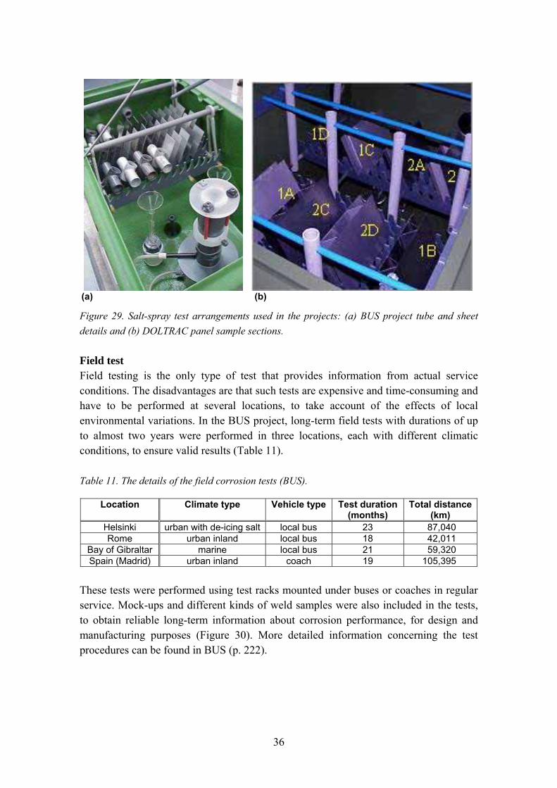
The environmental cycles and salts used in salt-spray tests can be varied according to the application. In the BUS project, the salt-spray tests, with a test duration of 500 h, were defined to simulate corrosive de-icing conditions on winter roads in certain locations, whereas in the DOLTRAC project, sodium chloride (NaCl) was used in the tests. In both cases, the tests were performed not only with base materials but also included samples with different types of welded joint (MAG, TIG, laser, spot, weldbonding), structural condition (sheet, lap and butt joints, hydroformed, hollow sections, sandwich panels), surface treatment (as-welded, pickled, brushed), etc. (Figure

29). More detailed information concerning the test procedures and complete results can be found in BUS (p. 199) and DOLTRAC (p. 203).

36

(a) (b)

Figure 29. Salt-spray test arrangements used in the projects: (a) BUS project tube and sheet

details and (b) DOLTRAC panel sample sections.

Field test Field testing is the only type of test that provides information from actual service conditions. The disadvantages are that such tests are expensive and time-consuming and have to be performed at several locations, to take account of the effects of local environmental variations. In the BUS project, long-term field tests with durations of up to almost two years were performed in three locations, each with different climatic conditions, to ensure valid results (Table 11).

Table 11. The details of the field corrosion tests (BUS).

Location Climate type Vehicle type Test duration Total distance (months) (km)

Helsinki urban with de-icing salt local bus 23 87,040 Rome urban inland local bus 18 42,011

Bay of Gibraltar marine local bus 21 59,320 Spain (Madrid) urban inland coach 19 105,395

These tests were performed using test racks mounted under buses or coaches in regular service. Mock-ups and different kinds of weld samples were also included in the tests, to obtain reliable long-term information about corrosion performance, for design and manufacturing purposes (Figure 30). More detailed information concerning the test procedures can be found in BUS (p. 222).

37

(a) (b)

Figure 30. Photograph from the test racks and specimens used in the long-term field tests: (a) a

readily assembled rack and (b) a rack installed underneath a bus (BUS).

2.4.4 Corrosion test results

Ferritic stainless steels The atmospheric corrosion resistance of ferritic stainless steels is directly proportional to the chromium content of the alloy. Type EN 1.4003 is not recommended for outdoor architectural applications, due to its poor localised-corrosion resistance – which causes surface staining, even in rural conditions, unless protected with coatings. The same applies to its use in vehicle-chassis structures, as the results of the salt-spray and field tests showed (Figure 31, Figure 33 and Table 12). Welding further reduces the localised-corrosion resistance of EN 1.4003. Its corrosion resistance can be improved by post-weld surface treatments such as pickling, which, together with shot peening, gives the best results (Kyröläinen et al. 2000). Although EN 1.4003 is not recommended for outdoor architectural applications, due to its poor localised-corrosion resistance, it has successfully been used in open train wagons for bulk transport. This low-alloyed stainless steel showed lower life cycle costs than wagons made of painted steel, that required severe maintenance work every 8-10 years (Atlas Specialty Metals 2008).

Recently, ferritic stainless steels with higher chromium content, with or without molybdenum, have been developed and adopted for vehicle applications. The corrosion resistance of EN 1.4521, with 18 % Cr and 2 % Mo, for example, is expected to be similar to that of EN 1.4401 austenitic stainless steel. Furthermore, ferritic stainless steels with 17 % Cr and 1.5 % Mo (e.g. 1.4113, 1.4526) are being used in automotive trims. Ferritic stainless steels should also be considered when there is a risk of chloride-induced stress corrosion cracking, since they are virtually immune to it.

38

(a)

(b)

(c)

d)

Figure 31. Localised corrosion and staining of powder plasma arc welded (PPAW) and

weldbonded (WB) EN 1.4003 2B after 500-hour salt-spray test in CaCl2 at 20 °C. (a) PPAW

before and after 500-hour test, not pickled, (b) PPAW before and after 500-hour test, pickled,

(c) WB before and after 500-hour test, not pickled, (d) WB before and after 500-hour test,

pickled (BUS).

39

Austenitic CrNi and CrNiMo stainless steels Austenitic grades EN 1.4301 with a minimum of 17.5 % Cr and 8 % Ni and EN 1.4401 (minimum 16.5 % Cr, 10 % Ni and 2 % Mo) have good atmospheric corrosion resistance and have been successfully used for decades in various architectural applications. According to laboratory tests, field tests and practical experience, EN 1.4301 grade should provide adequate atmospheric corrosion resistance in most vehicle applications (Figure 32, Figure 33 and Table 12). Apart from remaining intact in urban atmospheres, it should also remain practically intact in marine atmospheres and even, when properly treated, in urban atmospheres in the presence of de-icing salts (Figure 33(d)). Welding reduces corrosion resistance and can lead to pitting corrosion and staining in the presence of chlorides, originating from sources such as seawater mist, rainwater, de-icing salts or dust-control chemicals. Laser welding gives better corrosion resistance than arc or spot welding. Excessive heat input is detrimental. Corrosion resistance can be restored by post-weld surface treatments – again pickling provides the best results.

Molybdenum and nitrogen alloying improve pitting-corrosion and crevice-corrosion resistance. This was clearly seen both in the salt-spray and field tests, where grade 304SP, with 0.8 % Mo and 0.1 % N, was superior to standard grade EN 1.4301, both in as-welded condition and after pickling (Figure 34 and Table 12).

Based on the nitrogen content, the corrosion resistance of grade EN 1.4318, with minimum 17 % Cr, 6 % Ni and 0.1 % N, should be equal to or even slightly better than that of standard grade EN 1.4301. This assumption is supported by salt-spray tests on sandwich panels. Grade EN 1.4310 has also been successfully used in railway cars and truck trailers. In building applications, grade EN 1.4310 is reported to suffer from rust staining in the presence de-icing salts.

The risk of crevice corrosion can be minimised by careful design. Butt joints should be preferred to lap joints and, if lap joints are used, weld bonding should be preferred to spot welds. Although weld bonding itself can prevent crevice corrosion, pickling is still required to restore the corrosion resistance of the outer surfaces, as shown in Figure 32(c) and (d). Pickling must be performed with care, to avoid deterioration of the adhesive in the joint.

Surface finish has a major effect on localised-corrosion resistance in atmospheric applications. Smoother surfaces retain less dirt and deposits and provide better resistance against pitting corrosion, surface staining and tarnishing than do rough surfaces. This was clearly seen in the salt-spray tests, where the colourisation of both 1D and brushed surfaces was more intense than that of the smoother 2B finish (BUS p. 199).

40

According to the salt-spray and field tests, strength level (2B compared to 2H) has no marked influence on localised-corrosion resistance in atmospheric exposure. Heavy cold working or straining of metastable grades, which would cause the formation of strain-induced martensite, may expose these materials to hydrogen embrittlement when in contact with, galvanised steels. Stable grades are not susceptible to this type of degradation.

(a)

(b)

(c)

(d)

Figure 32. Localised corrosion and staining in welded EN 1.4301 2B after a 500-hour salt-

spray test in CaCl2 at 20 °C. (a) PPAW – before and after 500-hour test, no pickling. (b) PPAW

– before and after 500-hour test, pickled. (c) Weld bonded – before and after 500-hour test, no

pickling. (d) Weld bonded – before and after 500-hour test, pickled (BUS).

41

Figure 33 shows the behaviour of ferritic 1.4003 and austenitic 1.4301 materials in various field-test environments. Although these specimens have been powder plasma arc (PPAW) welded, it has been demonstrated in the BUS project that the difference in corrosion behaviour as compared to MIG/MAG welding is negligible (Table 12).

(a)

(b)

(c)

42

(d)

Figure 33. The effect of atmospheric exposure on the localised-corrosion behaviour of EN

1.4003 (left) and 1.4301 (right) PPAW welded and pickled 40×40×1.5 SHS specimens. (a)

Rome: 42,011 km. (b) Madrid (coach): 105,395 km. (c) Gibraltar: 59,320 km. d) Helsinki:

87,040 km (BUS).

(a) (b)

Figure 34. Localised corrosion and staining in grade 304SP after a 500-hour salt-spray test in

CaCl2 at 20 °: (a) PPAW no pickling after welding and (b) weld bonded, no pickling (BUS).

Austenitic CrMn stainless steels At present, there is only a limited amount of published test data concerning the use of manganese-alloyed austenitic stainless steels in vehicles. In general, the atmospheric-corrosion resistance of Mn-alloyed grades should be equal to that of CrNi grades with a similar chromium content. This assumption is in line with the tests performed in the BUS project, which showed that the localised-corrosion resistance of 16-7Mn grade, with 16.5 % Cr, 7.4 % Mn and 0.19 % N, was comparable to or only slightly lower than that of the standard CrNi grade EN 1.4301 (Figure 32, Figure 35 and Table 12). These results are also in agreement with previous literature references, which state that type AISI 201 manganese-alloyed stainless steel, with 16-18 % Cr and 0.25 % N, can be successfully used in railway carriages. Welding reduces corrosion resistance and materials to the risk of pitting corrosion and staining, as in the case of CrNi-alloyed grades. Corrosion resistance can be restored by post-weld surface treatments (Figure 35 (a)).

43

(a)

(b)

Figure 35. Localised corrosion and staining in grade 16-7Mn 2B sp after a 500-hour salt-spray

test in CaCl2 at 20 °C: (a) PPAW no pickling (left) and with pickling (right) after welding and

(b) weld bonded, no pickling (left) and with pickling (right) (BUS).

A compilation of the field corrosion-test results, based on visual inspection, are shown in Table 12. More detailed information on the tests and their results can be found in BUS p. 222.

Table 12. Corrosion behaviour of different stainless steel grades in various ground transport

service conditions based on the long terms field tests (BUS p. 222). A hyphen (-) indicates that

no test data is available from the projects.

Material, joint type, condition Urban Marine

Inland De-icing salts

Coach Spain Rome Helsinki Gibraltar

EN 1.4003, 2B BM W BM W BM W BM W

Spot-welded lap W 3 5 0(**) 2(**) 5 5 3 3 P - - 1(**) 0(**) - - - -

Weldbonded lap W 4 5 1 3 - - 3 3 P - - 2 0 5 5 - -

PPAW butt W 4 5 2 3 5 5 4 5 P - - 0 0 - - - -

Laser-welded butt W 4 5 - - - - 4 4 P - - - - 5 5 - -

Hydroformed F - - - - 5(*) - - - P 4(*) 4(*) - - 4(*) - 3(*) 3(*)

EN 1.4301, 2B BM W BM W BM W BM W

Spot-welded lap W 2 2 - - 3 2 0 0 P - - - - - - - -

Weldbonded lap W 1 1 0 2 3 3 0 0

44

Material, joint type, condition Urban Marine

Inland De-icing salts

Coach Spain Rome Helsinki Gibraltar P - - 1 0 3 2 - -

PPAW butt W 2 2 0 1 3 4 0 1 P - - 0 0 - - - -

Laser-welded butt W 2 1 - - 3 2 0 1 P - - - - - - - -

Hydroformed F - - - - 2 - - - P 2(*) 2(*) - - 1 - 1(*) 1(*)

304 SP, 2B BM W BM W BM W BM W

Spot-welded lap W 1 1 0 1 3 3 0 0 P - - 1 0 - - - -

Weld bonded lap W 0 0 0 0 - - 0 0 P - - 0 1 3 2 - -

PPAW butt W 1 1 1 1 3 4 0 1 P - - 0 0 - - - -

Laser-welded butt W - - - - 3 2 - - P 1(.) 1(.) - - 2 1 0(.) 0(.)

Hydroformed F - - - - - - - - P - - - - - - - -

16-7Mn, 2B BM W BM W BM W BM W

Spot-welded lap W 1(**) 1(**) 1(**) 2(**) 3 2 1(**) 1(**) P - - - - - - - -

Weldbonded lap W - - - - - - 0(**) 1(**) P - - - - - - - -

PPAW butt W - - 1 2 3 2 1(**) 4(**)P - - - - - - - -

Laser welded W - - - - - - - -P - - - - 2 2 - -

Hydroformed F - - - - 3 - - -P - - - - 2 - 1 0

W = as-welded/bonded P = pickled (*) Gauge: 2 mm (**) Gauge: 3 mm (.) Steel brush (L)

Codes: 0 = No colouring 1 = Only small coloured spots 2 = Mild local colouring or corrosion (< 5% of the surface)

3 = Colouring or local corrosion (5-25% of the surface) 4 = Colouring or accelerated corrosion (25-75% of the surface) 5 = Whole surface coloured or corroded

2.4.5 Corrosion test summary

It should be noticed that no general rules can be generated based on the results of individual projects because of the complexity of the subject. Therefore, the results presented in this handbook should be regarded as indicative only. Furthermore, the harshness of the salt-spray tests should also be taken into account: as described earlier, they generate a well defined, highly corrosive environment that is reproducible for comparing and ranking the corrosion resistance of different stainless steel grades in a qualitative sense. However, it is not possible to make quantitative comparisons or corrosion-resistance measurements. The results are seldom transferable to actual service life, since the test does not normally reproduce true in-service conditions (ISSF 2008). Also, the corrosion effects in stainless steels in the tests presented here usually merely

45

visual and not detrimental to structural performance. Here is a brief summary of the project corrosion tests:

Salt spray tests Base materials (BUS)

- Austenitic grades tend to stain without, however, developing structurally relevant corrosion damage.

- Corrosion effects affect appearance but are not detrimental to structural behaviour.

- For the above, surface defects are preferential sites for the growth of defects. - No clear difference is observed between 2B and 2H surfaces.

Joints (BUS) - Oxidation, then staining/colouring appear in all types of joints. - Pickling or brushing reduces the risk of oxidation. - Lap joints show a risk of crevice corrosion in all steels but 304SP (Mo-alloying). - Butt laser welds appear to be the most effective joints.

Panel section salt-spray tests (DOLTRAC) - In general, no significant surface damage, other than that caused by surface

heterogeneity such as spots, marks or scratches, is found in the tested panel samples.

- Both as-welded and pickled joints give the same good result. - Non-pickled samples with a continuous weld do not undergo important changes,

keeping their original quality except for a little oxidation due to the edge effect. - Observation of the cross-sections of joints showed that the gap between

sandwich parts may vary. Incomplete sealing permits the entry of an electrolyte solution. The difference in oxygen access through the lap area and the rest of the joint in contact with the solution would be a major factor in explaining the occurrence of corrosion in the different joints. A properly sealed joint would avoid crevice corrosion.

Field corrosion tests (BUS) Base materials

- Ferritic grade 1.4003 shows a risk of corrosion (colouring, pitting, crevice) in on-road conditions when chlorides are present (de-icing, marine atmosphere), if used without protection (painting or other types of coating).

- Austenitic grades 1.4301 and 16-7Mn also show a risk of colouring and pitting corrosion from surface defects (rough finish) and oxidation caused by welding.

46

- Molybdenum-alloyed type 304SP also colours as a result of weld oxidation but the risk of pitting corrosion is significantly smaller than in the case of the other steels.

- No effect on colouring and corrosion is observed with 2B and 2H surfaces.

Joints - Lap joints show a risk of crevice corrosion. - Crevice corrosion can be avoided by eliminating crevices (design, sealing,

coating) and/or by using molybdenum-alloyed steels. - Weldbonding is a potential technology for avoiding crevice corrosion. - Type 304SP is less prone to crevice corrosion than 1.4301. - The oxidation caused by arc welding involves a corrosion risk that can be

avoided by pickling or brushing the weld bead.

2.5 Stainless steel high-temperature mechanical properties: fire resistance

The stress-strain relationships of stainless steel at elevated temperatures must be understood in order to determine the load-bearing capacity of a structure under fire conditions. Tests to determine mechanical properties at elevated temperatures are classed as “steady-state” and “transient-state”. In the traditionally used steady-state tests, the temperature is kept constant, while in transient-state tests it is the load that remains unchanged. The transient-state test is claimed to give a more realistic description of a material’s behaviour in fire conditions. The difference between the stress values established using different test methods depends on the temperature considered. When comparing the results of cold-formed materials, it is important to pay attention to the fact that the degree of material deformation (i.e. the cold-worked material strength level) also affects behaviour at elevated temperatures.

Strength values are defined through so-called reduction factors – i.e. the ratio between elevated-temperature and room-temperature strengths. Figure 36 compares the reduction factor of stress in relation to proof strains of 0.2 % for EN 1.4301, in two different cold worked conditions, according to transient-state (Outinen & Mäkeläinen 1997) and steady-state tests (Ala-Outinen 1996).

47

Figure 36. Reduction factors of the yield strength of austenitic stainless steel EN 1.4301,

comparing the results of different methods used to test virgin sheet and cold-formed material

(Ala-Outinen & Oksanen, 1997).

The strength of a material increases due to cold working during the fabrication process. The remains of this increased strength at elevated temperatures can be seen in Figure 36. The increased strength due to the cold-forming process remains more or less constant up to 600 °C but beyond this point strength begins to decrease and the influence of cold-forming totally disappears at 900 °C.

Since the various stainless steel types behave differently, it is reasonable to determine the specific reduction factors separately for each type of stainless steel. Furthermore, both tensile strength and elastic modulus behave similarly to proof strength at elevated temperatures. However, determining the modulus of elasticity based on the slope of the stress-strain curve is very inaccurate, as the proportional limit of austenitic stainless steel is very low. The least inaccuracy in the measured curves has a very significant influence on the calculated modulus of elasticity and the unreliability of modulus-of-elasticity values determined in this way is thus quite remarkable.

Table 13 shows the reduction factors of yield strength in relation to 0.2 % proof strain for various stainless steel grades and various delivery conditions. Further data on the fire properties of the various stainless steel grades and forms are given by Ala-Outinen (1996), Ala-Outinen et al. (2003), Outinen & Mäkeläinen (1997) and Baddoo & Burgan (2008).

0

0.1

0.2

0.3

0.4

0.5

0.6

0.7

0.8

0.9

1

0 100 200 300 400 500 600 700 800 900

Temperature [C]

Red

uct

ion

fac

tor

Steady-state tests, Base mat. Transient state tests, Base mat.

Steady-state tests, RHS-tubes Transient state tests, RHS-tubes

48

Table 13. Numerical values of the reduction factors of 0.2 % proof strength of various stainless

steel grades and conditions (Euro Inox 2006b).

Temperature Rp0.2 reduction factor (°C) 1.4301 1.4318 1.4003

2B 2B C850 20 1.00 1.00 1.00 1.00

100 0.82 0.78 0.86 1.00 200 0.68 0.65 0.77 1.00 300 0.64 0.57 0.69 0.98 400 0.60 0.51 0.68 0.91 500 0.54 0.48 0.65 0.80 600 0.49 0.46 0.54 0.45 700 0.40 0.40 0.40 0.19 800 0.27 0.27 0.23 0.13 900 0.14 0.11 0.10 1000 0,06 0.07 1100 0.03 0.035 1200 0.00 0.00

Figure 37 demonstrates the difference between the fire behaviour of different austenitic stainless steel delivery conditions, stainless steel types and stainless and aluminium alloys. The curves are based on the above reduction factors and the project material data given in Chapter 2.3.1, except for Type 1.4318 2B, for which EN 10088-2 values are used. Aluminium alloy data is from Aluminium Taschenbuch (1988).

Figure 37. Proof stress temperature-dependency of various stainless steels and aluminium

alloys.

0

100

200

300

400

500

600

0 200 400 600 800 1000 1200

Temperature (°C)

Pro

of

stre

ss R

p0

.2 (

N/m

m2 )

1.40031.4318 2B

1.4318 C8505083 W287075 F53

49

It is typical of cold-worked stainless steel that the strength difference resulting from cold working remains up to about 600 °C but decreases rapidly beyond that point, so that there is virtually no strength advantage left at 900 °C. The ferritic grade retains its room-temperature strength longer than the austenitics but drops below their level at around 700 °C. For the aluminium alloys, the collapse in strength values occurs at considerably lower temperatures than in the case of stainless steels. This is understandable, considering the low melting temperatures of these alloys below 600 °C. There are no significant differences between the AlZnMgCu alloy EN-AW 7075 and the lower-alloyed AlMgMn alloy EN-AW 5083, despite the fact that the former has considerably higher room-temperature strength.

2.6 Selection of materials

The well-established and multipurpose CrNi-grade 1.4301 (AISI 304) is often used as a basis for the process of stainless steel material selection. Fluctuating raw-material prices have led to a reconsideration of materials used. New alloys, such as new, leaner duplex grades (e.g. 1.4162) and ferritic grades with increased chromium content (e.g. 1.4509), have increased the interest in looking more thoroughly at these alternative materials. In addition, low-nickel austenitic grades (e.g. 1.4318) and the re-discovered CrMn-grades (e.g. 1.4372) have emerged in recent years. Several papers and articles on ferritic grades or the 200 series (including substitution stories) have accordingly been published, emphasising a wide variety of substitution strategies and material alternatives that should be studied and tested before material replacement (Charles 2005, Osima 2007, Singhal 2007, ISSF 2007, Schwind 2008).

2.6.1 Structural applications

The use of stainless steel in structural applications has been growing steadily, as explained in the first chapter of this handbook. As well as growth in transportation applications, growth in the building and construction segment is taking place and the design guidelines for stainless steel have accordingly been developed (Euro Inox 2006b, Baddoo 2007).

Given a proper material-selection process, it is possible to find an optimal combination of strength and corrosion resistance. Table 14 lists some stainless steel grades that can be considered as alternative materials to the common 1.4307 (AISI 304L) grade. All these materials have a lower nickel content than grade 1.4307, resulting in less volatile prices. The price level of the lowest-alloyed grade (1.4003) is typically about 0.5 - 0.7 times that of the listed austenitic and duplex grades.

50

Table 14. Typical chemical compositions of some stainless steel grades for structural

applications. The pitting resistance equivalent (PRE) is calculated according to the formula

PRE=Cr(wt-%)+3.3×Mo(wt-%)+16×N(wt-%). Steel designations according to

EN 10088-2:2005, EN 10088-4:2005 and ASTM A240-07 (Taulavuori 2008).

EN ASTM C Cr Ni Mn N Fe Note PRE

1.4307 304L 0.02 18.2 8.1 1.5 0.05 Bal.Ni enhances repassivation

19

1.4318 301LN 0.02 17.6 6.5 1.2 0.15 Bal.Ni enhances repassivation

20

1.4372* 201 0.02 16.8 4.5 7.0 0.20 Bal.Cr level to be kept

high and S level low 20

1.4162 S2101 0.02 21.5 1.5 5.0 0.22 Bal.Duplex structure, lean composition

25

1.4003 S40977 0.02 11.5 0.4 1.3 0.02 Bal.Low-alloyed ferritic

grade 12

*Typically produced with a higher carbon content of 0.05 %

The carbon content of structural materials should be below 0.03 % when materials with a wall thickness of over 6 mm are to be welded with conventional fusion-welding methods. In order to prevent staining and pitting corrosion in outdoor applications, it is advisable to select a steel grade with a pitting potential equivalent (PRE) of about 20 or higher. Otherwise, a protective coating has to be applied. Superficial corrosion in coastal, industrial and polluted urban areas can be avoided by using even higher-alloyed grades than those listed in Table 14.

As the numbering system of stainless steels is based on their chemical composition, it is difficult to get an idea of the mechanical properties of a grade only on the basis of its name. Standardised minimum values for different grades are therefore shown in Table 15. It can be clearly seen that all presented alternatives to grade 1.4307 have higher yield strength and higher tensile strength, although their greater price stability is due to lower nickel content. Nitrogen-alloyed austenitic grades usually have a 1.5-times higher yield strength, and duplex grades a 2-times higher yield strength, than grade 1.4307.

Table 15. Minimum values for cold rolled strip (transverse to the rolling direction) according to

EN 10088-2:2005, EN 10088-4:2005 and ASTM A240-07.

EN grade

AISI/UNS grade

Rp0.2 (N/mm2) Rm (N/mm2) A (%) EN ASTM EN ASTM EN ASTM

1.4307 304L 220 170 520 485 45 40 1.4318 301LN 350 240 650 550 40 45 1.4372 201LN 350 310 750 655 45 45 1.4162 S32101 530 530 700 700 30 30 1.4003 S40977 320 280 450 450 20 18

51

Thermomechanical treatments can be considered as a method for further increasing the use and competitiveness of stainless steels. Even basic CrNi grades can be hard cold rolled to a desired strength level, to optimise their mechanical properties. These cold worked, temper rolled grades are widely standardised both in Europe and in the U.S.A typical yield strength level of 500 to 700 N/mm2 is widely used in the production of railway cars, for example, as mentioned earlier.

In addition to cold working, other strengthening methods such as bake hardening (i.e. the strain-ageing phenomenon) have been studied intensively since the 1990’s (Murata 1993, Karjalainen 2008). A strength increase of 100 N/mm2 is possible with commercial austenitic stainless steels such as grade 1.4301 by bake hardening. When the right combination of steel grade and cold working prior to bake annealing is chosen, the strength increase can be well above 200 N/mm2. As the annealing temperature can be kept below 200 °C, thus avoiding heat tints even without using shielding gas, bake annealing is easily adapted to many cases where the strength of a deformed material is to be increased.

2.6.2 Forming applications

The standardisation of CrMn grades is in progress in several countries and regions worldwide, leading to some inconsistency in the properties of material supplied by different producers and some availability difficulties. Certain 200-series grades from Far Eastern producers, in particular, do not meet the requirements of the European or U.S. markets (Charles 2005). In Europe, the use of CrMn grades has increased, but there is uncertainty on several scores, including:

• Corrosion resistance (e.g. chromium and sulphur content) • Formability (e.g. austenite stability) • Scrap value (e.g. manganese and copper content) • Availability (incl. variations between different producers and even between lots)

The most widely used standard composition of CrMn-grades is currently grade 1.4372/AISI 201, as listed in Table 16. The considerable interest in these materials has led to the development of grades containing increased chromium and nickel levels (of 17 % and 4 % respectively), to meet general requirements for materials in contact with food (Technical 2001).

52

Table 16. The typical chemical composition of some stainless steels suitable for forming

applications. Grades 201Cu and 204Cu are Cu-bearing grades and are not mentioned in ASTM

A240 as such. The pitting resistance equivalent (PRE) is calculated according to the formula

PRE=Cr(wt-%)+3.3×Mo(wt-%)+16×N(wt-%). Steel designations are according to EN 10088-

2:2005 and ASTM A240-07.

EN AISI / UNS C Cr Ni Mn Cu N Fe PRE 1.4301 304 0.04 18.2 8.1 1.4 0.3* 0.05 Bal. 19 1.4372 201 0.05 17.2 4.5 6.5 0.3* 0.20 Bal. 20 1.4618 “201Cu” 0.05 17.2 4.5 6.0 2.0 0.10 Bal. 19

1.4597 “204Cu” 0.06 0.10

16.5 15.2

2.2 1.2

7.0 8.7

2.2 1.7

0.20 0.11

Bal. Bal.

20 17

1.4509 S43940 0.02 18.0 0.2* 0.4* 0.1* 0.02 Bal. 18 1.4016 430 0.04 16.2 0.2* 0.4* 0.1* 0.03 Bal. 16

*Typical residual level of the element

The ferritic grades listed in Table 3 are the conventional grade 1.4016, with good availability on the stainless steel markets, and the emerging grade 1.4509, seen by many as an updated version of grade 1.4016 for applications where better corrosion resistance and weldability are required. In general, ferritic grades have the advantage over austenitic grades in terms of mechanical properties. Less prone to springback effects, they are also easier to cut and work.

Table 17 shows the mechanical properties of certain stainless steels suitable for forming applications. All the austenitic grades have rather similar mechanical properties. The higher yield strength of some CrMn grades is not detrimental to their formability, thanks to their high elongation-to-fracture values and moderate work-hardening behaviour compared to the other austenitic grades. This can be seen in Table 18, where all the CrMn grades reach deep drawing ratios of over 2. The main concern is a phenomenon called “delayed cracking” or “seasonal cracking”, which has been reported for almost all manganese-alloyed materials and which occurs within a few minutes to several days or even weeks after forming. The nickel content of the steel and the deep drawing ratio correlate clearly when delayed cracking is reported. However, since deep drawing is not often used in the fabrication of rail coaches and buses, delayed cracking is not normally a point of concern in these applications.

53

Table 17. The minimum values for cold rolled strip (transverse to the rolling direction)

according to EN 10088:2005 and ASTM A240-07. Grades 201Cu and 204Cu are Cu-bearing

grades and are not mentioned in ASTM A240 as such. The typical values are only informative

and the range is collected from various sources and test data.

EN AISI / UNS

Rp0.2 (N/mm2) Rm (N/mm2) A80 (%) Global standardisationEN Typical EN Typical EN Typical

1.4301 304 230 280-300 540 600-700 45 50-60 Fully

standardised 1.4372 201 350 350-420 750 650-800 45 45-60 Well established

1.4618 “201Cu” (220) 300-400 (520) 550-700 (40) 40-60 Recently

established 1.4597 “204Cu” 300 350-450 580 750-950 40 30-50 In progress 1.4509 S43940 250 280-350 430 500-600 18 20-30 Well established

1.4016 430 260 300-360 450 480-500 20 20-30 Fully

standardised

Table 18. The sensitivity to delayed cracking of some austenitic steels in relation to the Limit

Drawing Ratio, measured by Swift Cup Test (Taulavuori 2008).

Swift Cup Test / Limit Drawing Ratio Grade Ni % Cu % 1.4 1.6 1.8 2.0 2.12 2.14

1.4301 8.1 0.5 + + + + + + “201Cu” 4.7 2.4 + + + + + 1.4372 4.4 0.3 + + + -- -- -- 1.4372 3.6 0.3 + + -- -- -- -- “204Cu” 1.1 1.7 + -- -- -- --

+ = Successful -- = Delayed cracking

2.6.3 Summary

Volatile nickel prices have made both users and producers of stainless steel seek for alternative materials to the conventional CrNi grades. In 2007, especially, reactions to raw-material price developments were relatively strong. It can nevertheless be clearly seen that classic grade 1.4301 (AISI 304) will continue to be used in many applications, thanks to its multifunctional properties. Several grades already exist, however, that provide enhanced properties and greater price stability in certain applications, compared with grade 1.4301.

In structural applications, manganese and nitrogen alloying and the use of the duplex or pure ferritic structure are alternatives. Novel thermomechanical treatments, including cold working by temper rolling, can also be taken into consideration. For forming applications, there are a few CrMn grades and ferritic grades that are worth considering, especially when grade 1.4301 may be an over-specification. An overview on optimising production processes by the selection of materials and processes is given in Figure 38.

54

Figure 38. Optimising both material and manufacturing costs by using new alloys and novel

treatments (Taulavuori 2008).

1.4301AISI 304

Structural Applications

Forming Applications

PriceStabilityThroughAlloying

PriceStabilityThroughAlloying

Thermo-MechanicalTreatments

OptimizedHeat-Treatments

301LN1.4318

N

201LNN & Mn

DuplexN & Mn

1.4162

Ferritic1.4003

Cr 12 % TemperRolling

TemperRolling

&BakeHardening

TemperRolling

&Reversion

Annealing

Mn1.4372

201

Mn & Cu 1.4618

“201Cu”&

“204Cu”

Ferriticgrades:

1.4509Cr 18 %

&1.4016

Cr 16 %

Inter-

mediateAnnealing

Local

Heatingto Prevent

HardeningHot

FormingProcesses

55

3. Lightweight structures and design

Most stainless steel structures in transport vehicles are made of hollow sections. Examples include bus-body frames and sheet-metal parts, either flat (e.g. bus-body surface sheets) or formed (e.g. roll-formed profiles in trains or metro cars). A relatively new technology, of great potential, is the use of all-steel sandwich panels. It offers the possibility of massive weight reduction. This chapter briefly reviews hollow-section and sandwich-panel design principles. Further information on the manufacturing of such structures will be found in Chapter 4, “Manufacturing issues in lightweight structures”.

3.1. Stainless hollow-section structures

This chapter discusses the manufacturing, dimension ranges and properties of stainless structural hollow sections readily available on the market. Apart from common “catalogue” or standard dimensions and materials, hollow sections may also be purchased in other materials and tailored dimensions, depending on the manufacturer´s capabilities. A more thorough presentation of standard stainless steel hollow sections and their manufacturing and applications can be found in a recent handbook (Yrjölä 2008).

3.1.1. Manufacture of hollow sections

Structural hollow sections are usually made by cold forming and welding. Cold forming is carried out either by roll forming or by bending separate hollow sections. Welding methods used are TIG or plasma arc welding, HF (high frequency induction welding) and laser welding (Yrjölä 2008).

Roll forming Roll forming is a continuous manufacturing method, in which steel strip is cold-formed on the production line using a number of roll-pair stands. The material used is coiled steel strip, longitudinally cut to the width corresponding to the dimensions of the hollow section. The steel strip is uncoiled, welded to the previous strip and fed to the roll-forming line. If required, strip-edge quality can be improved by edge trimming before forming. There are two different forming methods for square and rectangular hollow sections: round forming or direct forming.

In round forming, steel strip is first formed into a circular hollow section then welded and formed with profiling rolls into a circle, square or rectangle. Steel strip can also be directly formed into a rectangle, by bending it from the corner zones and welding the seam. The latter method is used when manufacturing hollow sections with large outer dimensions and/or in the case of small quantities.

56

After welding, the joint is finished by grinding. The quality of the weld is controlled by continuous non-destructive testing or, if required, by other methods (e.g. a flattening test). Structural hollow sections are cut to the desired length, bundled, strapped and either transferred to the shipping warehouse or sent for further processing. The hollow sections are identified by continuous inkjet marking and bundle-specific tags.

The mechanical properties of hollow sections change as a result of cold forming. These changes depend on the manufacturing method and the dimensions of the hollow section. The mechanical properties of a ready-made hollow section can be tested by making test specimens of the hollow section and by material-characterisation testing (Yrjölä 2008).

Production of single hollow sections In the case of single hollow sections, the base material is a cut sheet corresponding to the dimensions of the hollow section. The sheet is made circular using a press break machine, in a number of stages, after which the open profile is welded into a hollow section by a longitudinal weld, at a welding station. The weld and surface are finished at separate work stations. Steel strip can also be directly formed into a rectangle by bending it from the corner zones and welding the seam. These methods are used for manufacturing stainless structural hollow sections that cannot be produced by roll forming because of their dimensions or the size of the batch.

3.1.2. Structural design aspects for hollow-section joints

When designing joints and connections, several factors must be taken into account. For example, the mechanical strength and corrosion resistance of joints and connections must be ensured, the manufacture and inspection of the joints and connections must be properly carried out and defects due to difficult installation must be avoided. Furthermore, in welded joints and connections, particular attention must be paid to the following:

- Welds should be located outside high-stress and stress-concentration areas. - It must be possible to make all welds in the design. - It must be possible to carry out post-weld treatment, where appropriate.

In structural hollow-section constructions, joints used are usually T, K, N and Y joints and butt joints between hollow sections. Joints are most often welded at the workshop. Limit values for the geometry of load-transmitting welded joints are given in standard EN 1993-1-8 (2005) and instructions are published by CIDECT (1996). Bolted joints are usually used when components are joined on-site. Meshed joints and the possibilities offered by laser-beam machining have not been widely utilised in load-transmitting joints.

57

K joints The requirements for K joints in structural hollow-section constructions are that the connection angle between brace and chord should be greater than 30 °, that the gap g on the chord member surface between brace members must be sufficient and that joint eccentricity e (i.e. the point of connection of brace-member centre lines in the chord) is not too great. If these limit values are adhered to, load in the joint is distributed more evenly in the joint area.

Figure 39. A typical K joint between structural hollow sections (Yrjölä 2008).

Brace member welds that are transverse to the chord member can be made as fillet welds, when the joint angle θ is between 60 and 90 °. If the joint angle is less than 60 °, the side of the brace member facing the gap must be bevelled and welded as a butt weld (Figure 40). The opposite side is fillet-welded, in which case there must be sufficient throat thickness, even in the case of low connection-angle values. In this way, undersize welds on the load-bearing sides of the joint can be avoided.

Figure 40. The end of the brace member must be bevelled if the joint angle is θ ≤ 60 °. In this

case, the brace member facing the gap must be bevelled and the weld is made as a butt weld to

a semi-V groove (Yrjölä 2008).

Joint eccentricity e shows the intersection point of the brace members in proportion to the longitudinal axis of the chord member. With eccentricity values e ≠ 0 mm, a bending moment is created in the joint, which must be considered as a load on the chord

58

member. If eccentricity is greater than the limit value, this must be taken into consideration when estimating localised loads in the joint (Figure 41).

In design, a compromise must often be made when selecting eccentricity and gap g values. To make the joint, the minimum gap g value must be at least t1 + t2, where t1 and t2 are the thickness of the brace members connected to the joint. The minimum value defined for the gap ga between the weld toes of the joint is 1.5 times the chord-member’s wall thickness (CIDECT 1996). Defining a sufficient gap g and joint angle θ ensures that the joint can be made and inspected.

Figure 41. The impact of gap g between brace members on the eccentricity e of the joint (Yrjölä

2008).

In Figure 41, the joint angle is greater (60 ° ≤ θ ≤ 90 °). Thanks to the greater joint angle, the weld facing the gap is easier to make as a fillet weld, with sufficient throat thickness. However, greater joint-angle values also increase eccentricity e. In the figure on the right, decreasing the eccentricity e of the joint also leads to decreased gap g. Reducing the gap g value will lower the deformability of the joint, in addition to which too narrow a gap prevents proper welding. Both diagonals to be welded must always be welded separately, or an overlapping joint (Figure 42) must be used.

59

Figure 42. Overlapping joint (Yrjölä 2008).

The strength and rigidity of a joint can be improved by making the ends of the brace members’ joint overlap (Figure 42). Due to this overlapping, the brace member’s flanges also transfer load to the chord member. The chord member’s surface stresses are therefore less and the strength of the joint is defined on the basis of the effective cross-sectional surface of the brace members. It is recommended to weld the end of the brace member that remains invisible in overlapping joints.

T and Y joints In the case of T and Y joints, the joint between the brace member and the chord member is designed in the same way as in the case of K joints, when the load acts on the level of the brace and chord.

Figure 43. Typical loading of a T joint (Yrjölä 2008).

In the case of joints such as that in Figure 43, the load at the end of the joining member generates a shearing load and a torque load on the chord member, in addition to a bending load. Torque can be further divided into torsional and distortion load, affecting the cross-section of the chord member. Distortional load balances itself out, but it deforms the cross-section into a diamond shape (Figure 44). Distortional load causes

60

deformation of the cross-section, as well as additional stress components that must be taken into account in design. Distortion does not occur if the chord member is a round profile.

Figure 44. Loading causing distortion of the cross-section (left) and distorted member (right)

(Yrjölä 2008).

Figure 43 shows a structure in which the joined member is welded onto the side of the chord member, without stiffeners inside the chord member. There being nothing to prevent distortion of the chord member cross-section, the deformation shown in Figure 44 will occur.

Figure 45. Alternative ways to prevent cross-section distortion (Yrjölä 2008).

Figure 45 shows alternative ways of stiffening the cross-section, to prevent distortional deformations. On the left, the outer dimensions of the joining member are greater than those of the chord member and the lower corner of the member has been cut off. The joined member is welded either partially or fully around the chord, to stiffen the chord cross-section. In the centre, the chord is welded onto the transversal joined member. This is not a viable solution, in terms of chord strength. On the right, the joining member is smaller than the chord and is inserted into the chord. The opposite sides of the chord are perforated and the joined member is welded on both sides of the chord, using butt or fillet welds. Distortion in the cross-section can also be prevented by means of transversal plates welded inside the hollow section, but this is very difficult to carry out.

61

Another typical way to join a hollow section to a structure or to machinery is by using lugs. The most common function of a lug is to transfer loading from a machine (usually a hydraulic cylinder) or a mounting to a structural hollow section. The shape and location of the lug affect the strength of both the joint and the structural hollow section. For example, in Figure 46, if force F is placed to act at a distance of e = b from the centre of the profile the load does not cause distortion of the cross-section.

Figure 46. Principle and application of lugs (Yrjölä 2008).

If a load will not cause torque in the chord, the load can be transferred using a lug of the same height as the chord. Using a lug of equal height decreases deformation in the chord-member’s side wall (Figure 46 centre). If a load will cause torque in the chord, it is recommended to design a lug that will prevent cross-section deformation caused by loading, (Figure 46 right).

Hydroformed connectors An innovative way to avoid one of the most critical issues in hollow-section constructions (locating welds outside high-stress and stress-concentration areas) is to use pre-fabricated connector pieces. Using such pieces moves the welded joints away from the most critical areas: the joint corners. This is of particular importance in fatigue-loaded applications, such as transport vehicle structures.

62

Figure 47. A hydroformed stainless steel connector piece (left), a sketch of the joint

configuration (centre) and a welded joint (right) (BUS pp. 84 – 86).

Extensive work was carried out in the BUS project on manufacturing such connection pieces using hydroforming and on their structural applications (BUS p. 70). An example of a joint manufactured using a hydroformed connector can be found in Figure 47 and alternative connectors to hollow-section joint configurations in Figure 48.

Figure 48. Alternative connector pieces for hollow-section joint configurations (BUS p. 85).

3.2. Sandwich panel structures

The main advantage of all-metal sandwich panels is their improved strength-to-weight or stiffness-to-weight ratio, compared with a solid sheet or plate structure. This is due to the increase in “apparent” thickness of the structure, i.e. the outer surfaces being further away from each other. When the dimension in loading direction (i.e. the thickness) is a major factor in determining the resistance to that particular load, the increase in the structure’s thickness can be utilised directly as increased stiffness and load-bearing capacity. In an optimised panel, the core elements have the dual function of transferring the loads between the skins as effectively as possible while increasing panel weight as little as possible. In some cases, the weight-saving potential is huge and the panel weight per area can be reduced to a fraction of that of a solid sheet.

63

There are some disadvantages with all-metal sandwich panels. Firstly, manufacturing large panels with closed cross-section by welding usually requires a capital-intensive keyhole technique (typically laser welding). This leads to favouring mass production of standardised panels, which in turn decreases the possibility of economically weight-optimising small-volume structures. Secondly, the use of hollow-section or sheet-profile panel cores results in a heterogeneity of stiffness and strength properties between longitudinal and transverse panel directions that has to be taken into account in design. Thirdly, introducing feedthroughs or openings easily leads to breaking the otherwise continuous core element (or elements), which obviously affects the panel’s strength and stiffness. In view of these disadvantages, it is clear that the best areas for all-metal sandwich panels are weight-critical and load-carrying applications involving large areas of similar panels that require few or no feedthroughs. Train and metro-car floor structures are good examples of potential applications.

It has been shown that once a sandwich structure is designed to correspond to a conventional structure in terms of bending stiffness, weight reductions of up to 80 % are theoretically possible (Kujala et al. 2003). Taking into account other loading conditions, as well as the required joints and connections, actual weight reduction is less. For example, in some ship-industry applications the use of sandwich panels has resulted in weight reductions of up to 30 - 50 % compared to conventional steel beam structures (Kujala et al. 2003).

Sandwich panels with steel surface sheets and core are called all-steel sandwich panels. Typical all-steel sandwich panels can be subdivided, according to their core structure, into continuously-corrugated core panels and (individual) profile or hollow-section core-stiffened panels (Figure 49).

64

V-core

Vf-core

I-core

O-core

a) b)

Figure 49. a) Diagrams of the most typical all-steel sandwich panel types and b) examples of

finished profile and hollow-section core panels.

Interest in all-steel sandwich panels increased in the 1980s, as laser welding became more widespread. Laser welding offers excellent possibilities for manufacturing continuous joints in closed structures with outside access only, as in panel manufacture. Research into the development of all-steel sandwich panel design and manufacture has been carried out since the late 1980s and, today, Europe is the leader in all-steel sandwich panel technology, with the widest range of applications.

a) b)

Figure 50. a) Stainless steel sandwich-panel assembly using laser welding, b) semi-finished

panel with core elements welded to the top sheet.

65

New challenges have to be met in both the design and manufacture of sandwich panels, compared to conventional steel structures. Other than bending loads – for which the panels are most suitable – shear and point loading, which decrease the local strength of panels welded from thin sheet materials, must also be taken into account. Further theoretical strength challenges are introduced by joining and connecting the panels to each other and to structures.

New factors also have to be considered in panel manufacture. Manufacturing the core to tolerances sufficient to allow flatness in welded panels is a key prerequisite for panel applications. For this, joining methods other than arc welding, such as laser or resistance welding, adhesive bonding or mechanical joining, have to be used. These bring new possibilities but also introduce challenges and limitations to the design, manufacture, use and maintenance of panels (Kujala et al. 2003).

3.2.1 Design principles of sandwich panels

The structural design of all-steel sandwich panels can be divided into two parts: calculation of the elastic response of the structure and consideration of strength criteria. Figure 51 shows a chart of the design process according to Romanoff & Kujala (2002).

Figure 51. A schematic of the all-steel sandwich panel design process (Romanoff & Kujala

2002 p. 20).

The design of all-steel panels starts with defining panel geometry, loads, boundary conditions and strength criteria. Both main dimensions and core geometry are included in defining panel geometry. Main dimensions are generally length, width and thickness. Core geometry includes surface and core sheet thickness, core angles, etc. There are several measurements to describe core geometry, depending on the chosen core type.

66

Defining the loading case is a basic problem in panel design. Key load information includes location, type and magnitude. Apart from loads, boundary conditions are essential factors in structural behaviour – in design these may be either free edge, free support or stiff support. In practice, boundary conditions will be either free edge or something between free and stiff support. Apart from boundary conditions, it is also essential to define whether the structure will behave in a beam or plate-type manner. The strength criteria indicate the usability of the chosen structure with the chosen boundary conditions and loading cases (Romanoff & Kujala 2002, Kujala et al. 2003).

The stiffness properties of a panel are defined on the basis of the design starting/source data. Once this is established, panel response can be defined by elastic structural analysis. Elastic structural analysis will determine both panel stress and deformation state. Once the panel cross-section is known, the critical stresses and forces can be defined for the structure. The set strength and displacement criteria and the stresses and displacements in the structure can then be compared (Romanoff & Kujala 2002, Kujala et al. 2003).

3.2.2 Panel cross-section

As described earlier, there are several types of all-steel sandwich panel. The most common are so-called prismatic panels, where the core is formed by parallel elements stiffening the panel in a longitudinal direction (Figure 49). Cross-section variables include surface (front and back), sheet thickness, core sheet thickness, core width and height, distance between core elements, core flange width(s) and web angle. The benefits of prismatic panels include fast production and high stiffness-to-weight ratio, especially in the core (longitudinal) direction. In the direction transverse to the core, shear stiffness is relatively low. Because of this inhomogeneity, the panel works best as a beam, with its longitudinal axis coinciding with the beam axis (Kujala et al. 2003).

3.2.3 Elastic response

The procedure for calculating a panel’s elastic response depends on whether the structure is more like a beam or a plate in nature. Furthermore, whether beam analysis or 2D or 3D finite element analysis is used also has an effect. In practice, choice of method is governed by the required speed and accuracy of the analysis. Beam analysis is the fastest but least accurate method and 3D finite element analysis the slowest and most accurate. An exhaustive and detailed description of the design process can be found in Romanoff & Kujala (2002), but it usually consists of the following steps:

67

Stiffness parameters Despite the limitations in support conditions (the panel can only be supported from either two opposing edges or from one edge), the stiffness response of a point-loaded and longitudinally stiffened prismatic panel can often be evaluated with reasonable accuracy using beam theory.

Bending moments, shear forces and deflection The deflection of a sandwich structure consists of two components that result from bending moment and shear force. The total deflection of the structure is the sum of these two. Deflection calculations can be considerably simplified: with beams stiffened along their longitudinal axis, for example, simply defining the bending stiffness is often enough, since shear deformation will be negligible.

Stresses Once the shear force distributions are known, the shear stress distribution affecting the cross-section can be calculated. The stress calculation procedure is described in more detail in Romanoff & Kujala (2002).

3.2.4 Strength and deflection criteria

Strength criteria in panel design usually concern maximum allowable stresses, safety against buckling, maximum deflection and safety against local failure modes. Maximum allowable panel stresses are usually defined by fatigue strength or material yield strength. As for fatigue, the maximum stress level usually originates from joint design.

Yielding The Von Mises criterion can be used to determine yield strength but, in addition to global panel deflection, stress concentrations may also result from local loads. Depending on the nature of the loading case, local stress levels may be greater than global stress levels. As a result, a panel surface or core sheet may yield locally.

Global buckling Global buckling is a sudden increase of the deflection of the whole panel under compressive load. It should be noted that global buckling analyses are based on the assumption of an elastic material and totally planar beam or plate, which is not usually the case in practice. Initial deformation can be caused by welding during panel manufacture.

Local buckling Buckling of one of the individual panel parts (surface sheet or core) is called local buckling. Local buckling factors for different loading cases and boundary conditions

68

can be calculated using relatively simple formulas, which, together with some values for these factors, for various core geometries, are given in Kujala et al. (2003).

Deflections It is typical of space-critical structures that deflection is one of the dimensioning criteria. In such cases the elastic, global deflection of the structure must at no location exceed its set maximum value. A typical deflection criterion in design is L/300, where L is the web spacing of the structure.

Plastic failure The core may also fail locally as a result of local loads. There are calculation formulas for dimensioning for plastic failure in the literature reviewed in Romanoff & Kujala (2002).

3.2.5 Structural optimisation

The key task in any structural optimisation process is formulating the optimisation task itself, including defining the limits for the core dimension range to be optimised and defining strength and deflection criteria. In practice, the starting data includes the main dimensions of the structure, the loading applied to the panel and the boundary conditions (Kujala et al. 2003). From an optimisation point of view, it is essential to minimise the number of variables.

The optimisation task solution depends on how accurately details are calculated. A preliminary idea of core dimensions can usually be obtained by using analytical formulas, calculating through all the design alternatives possible with the parameters and finding the best solution in terms of weight or cost, for example. For more accurate analysis, 3D FEM can be used, but the optimum found may not be the global optimum.

An optimised solution usually lies close to the limits of the design criteria, so these limits have to be defined carefully. For example, the manufacturing technique defines the core thickness in an I-core panel – optimised core would be too thin to laser weld. Improving manufacturing techniques also leads to lighter-weight panels (Kujala et al. 2003). Figure 52 shows an experimental strucure manufactured for gaining practical experience with sandwich panels in actual service conditions (Alenius et al. 2002).

69

Figure 52. An experimental, sandwich-panel bus floor element, in grade 1.4003, assembled

using laser welding (Alenius et al. 2002).

3.2.6 Design tools

Several methods can be used for all-steel sandwich panel design, depending on the desired accuracy and speed. Available design methods and tools in ascending accuracy and time consumed are (Kujala et al 2003):

• readily available calculated design curves • beam theory together with analytical expressions for strength • 2D plate theory together with analytical expressions for strength • 3D FEM calculation for structural response together with analytical expressions

for strength • 3D FEM calculation for structural response and strength

The use of prepared design curves is by far the quickest design method. The designer needs to know the main dimensions and loading case of the panel. A suitable panel can be selected from several alternatives. A key benefit with design curves is that a rough estimate of a panel’s dimensions and geometry is available quickly and easily. On the other hand, the curves are connected to a particular core geometry and availability is limited (Kujala et al. 2003).

Panel response and strength can be solved with reasonable accuracy and in a reasonable time by using beam theory together with analytical expressions for strength. These make it possible to program formulas in closed form with a computer and enable the use of an optimisation programme that calculates through all the possible core parameter combinations defined (Kujala et al. 2003).

70

2D plate theory for response calculation together with analytical expressions offers an highly accurate and rapid design method for all-steel panels. The plate problem can be solved either with analytical expressions or 2D FEM. On the other hand, the designer can use a package developed for all-steel sandwich panels that automatically calculates the required stiffness parameters from the cross-section for FE programs (e.g. ESAComp).

The stress state affecting a structure can be estimated very accurately using 3D FEM, provided the supporting and loading geometry are known. Drawbacks of 3D FEM analysis include long modelling and calculation times and the fact that the results depend on the experience of the modeller (Kujala et al. 2003).

A structure can also be analysed totally with 3D FEM. Drawbacks of this design method are the experience required from the designer, long calculation times and a complicated modelling phase that also has to include the true material properties and contacts between different parts.

3.2.7 Special issues in all-steel sandwich panel design

Once the all-steel sandwich structure has been designed to endure the loads it will be subjected to, the designer still has to solve some specific sandwich-panel problems. These include point or impact-type loading, joint design between panel(s) and ambient structure, openings and feedthroughs, fire resistance behaviour and noise and vibration behaviour (Kujala et al. 2003).

Local strength of the surface sheet The aim of using a sandwich structure is to reduce structural weight. This often results in very thin surface sheets and it may be that the top surface sheet dents too readily, under point or impact loading. Simple, published calculation procedures make it possible to easily increase top-sheet thickness, which can be at least partially offset by increasing sheet strength (Kujala et al. 2003). An example of an application where impact resistance is important can be seen in Figure 53.

71

Figure 53. Stainless steel sandwich panels

used as side and floor elements of a gravel

trailer platform (Kenno Tech 2008).

Joints and feedthroughs A basic all-steel sandwich panel can be designed, for various purposes, using readily available design software packages. However, solutions for connecting the individual basic panels to each other and/or to ambient structures have to be solved on a case-by-case basis. Stresses must be transferred smoothly, without stress concentrations across the joints (Kujala et al. 2003). One specific problem is that of extending a panel in longitudinal direction, since this requires joints in both surface sheets and cores. These joints must be both high-strength and economical to manufacture. Furthermore, the fatigue strength of a structure is usually governed by joint behaviour. Feedthroughs penetrating the sandwich structure require a design of their own. Typically, a hole with reinforced edges is cut for this purpose. Preferably, feedthroughs should be located so as not to damage the core elements (Kujala et al. 2003).

Noise behaviour Because all-steel sandwich panels are lightweight structures, they usually do not have the mass to prevent noise penetration, especially at low noise frequencies. For this reason, noise isolation in most cases requires the use of separate, application-tailored insulation sheets (mats or equivalent).

73

4. Manufacturing issues in lightweight structures

The manufacturing of any structure obviously requires several steps and techniques that are at least partially common engineering knowledge. However, there are certain methods worth a closer look, due to the different behaviour of, specifically, austenitic-stainless and mild or low-alloyed steels. Regarding forming, anisotropy in cold formed austenitic stainless steel material requires particular attention, as explained in Chapter 2.3. Further information on the formability of stainless steels is given by Van Hecke (2006).

4.1 Bending of high strength stainless steel sheets

With conventional carbon steels, bending is usually carried out according to the data in DIN 6935 “Cold bending of flat rolled steels” (1975). This standard prescribes the minimum bending radii for a wide variety of steels. Austenitic stainless steels in general and especially the unstable grade 1.4318 exhibit higher strength than ferritic carbon steels and have different forming behaviour.

DIN 6935 ranks the available steel grades according to ultimate tensile strength, in three categories: Rm < 390 N/mm2, 390 < Rm < 490 N/mm2 and 490 < Rm < 640 N/mm2. A minimum bending radius is given for each category. The ultimate tensile strengths, as measured by a quasi-static tensile test using a single crosshead speed of 2.7 mm/min, and the corresponding minimum bending radii of the project materials, are given (where possible) in Table 19.

Table 19. Ultimate tensile strength and minimum bending radius according to DIN 6935 (1975).

Material t (mm)

Rm (N/mm2)

90 °

Rm (N/mm2)

90 °

rmin (mm)

0 °

rmin

(mm)

90 °

1.4318 2H/C1000 (301LN) 1.9 1119 1129 NA (4*) NA (4*)

1.4318 2H/C850 (301LN) 1 961 947 NA (1.6*) NA (1.6*) 1.4301SP 2B (304SP) 1 755 755 1.6 1.6 1.4318 2H/C1000 (301LN) 1.2 1070 1073 NA (2.5*) NA (2.5*) 1.4318 2H/C850 (301LN) 1.5 1055 1049 NA (2.5*) NA (2.5*)

*values in brackets are those of the highest strength category of DIN 6935

As can be seen from Table 19, the ultimate tensile strengths of most of the DOLTRAC materials are too high for the highest categories mentioned in DIN 6935. This standard is therefore not suitable for determining the minimum bending radius of the ultra high-strength grades investigated in this project. Rules of thumb for minimum bending radii of high-strength austenitic stainless steels are however given by Ordenbach (1989). The

74

values are shown in Table 20. A comparison between Table 19 and Table 20 shows that if the values in brackets are used (including those in the highest strength category), DIN 6935 values are too low for the C1000 grades and too high for the others.

Table 20. Minimum bending radii according to Ordenbach (1989).

Material t (mm) rmin (mm)

1.4318 C1000 (301LN) 1.9 4.75

1.4318 C850 (301LN) 1.0 1.0

1.4301SP 2B (304SP) 1.0 0.5

1.4318 C1000 (301LN) 1.2 3.0

1.4318 C850 (301LN) 1.5 1.5

4.1.1 Verification of minimum sheet bending radius

The minimum bending radius of the different grades has been investigated experimentally, using bending machines and tools with different radii. After bending, the outer surfaces of the samples were visually inspected for cracks. The results are summarized in Table 21.

Table 21. Outer surface of V-bends for various materials (DOLTRAC p. 49). RD = rolling

direction, TD = transverse direction, OK = no macro cracks, NOK = cracks.

Material Direction Bending radius (mm) R1 R1.5 R2 R2.5 R4 304SP 2B 1.0 mm RD OK - - - - TD OK - - - - 1.4318 2B 1.0 mm RD OK - - - - TD OK - - - - 1.4318 2H C850 1.5 mm RD OK - - - - TD OK - - - - 1.4318 2H C1000 1.2 mm RD OK - - - - TD OK - - - - 1.4318 2H C1000 1.9 mm RD OK - - - - TD NOK NOK NOK OK OK

Visual assessment of the outer surfaces is difficult, however. Only large cracks could be detected. Further bending investigations were performed using so-called T-tests. The principle is explained schematically in Figure 54. The figure preceding T describes the inner bending radius in terms of sheet-thickness multiples (e.g. for ½T the inner radius is 0.5 times the sheet thickness).

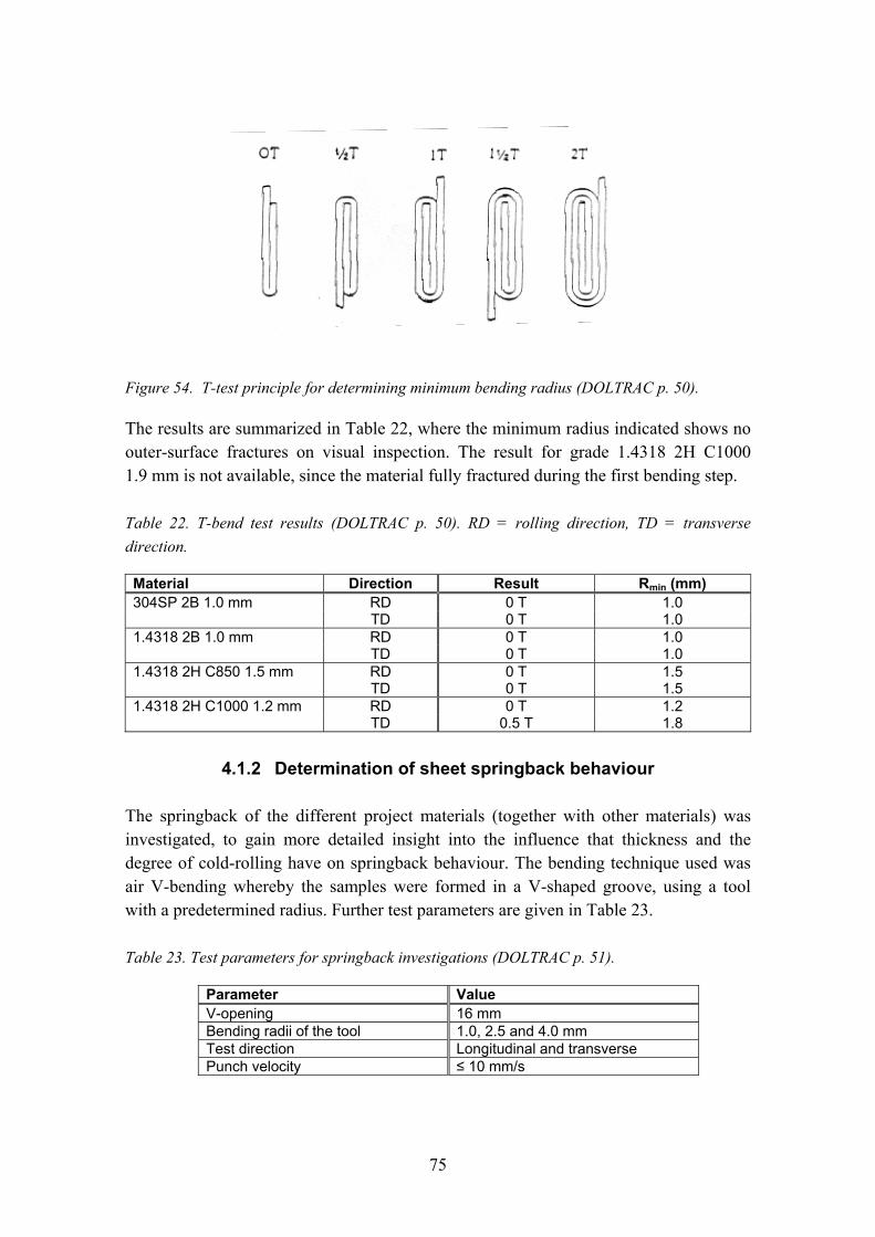
75

Figure 54. T-test principle for determining minimum bending radius (DOLTRAC p. 50).

The results are summarized in Table 22, where the minimum radius indicated shows no outer-surface fractures on visual inspection. The result for grade 1.4318 2H C1000 1.9 mm is not available, since the material fully fractured during the first bending step.

Table 22. T-bend test results (DOLTRAC p. 50). RD = rolling direction, TD = transverse

direction.

Material Direction Result Rmin (mm) 304SP 2B 1.0 mm RD 0 T 1.0 TD 0 T 1.0 1.4318 2B 1.0 mm RD 0 T 1.0 TD 0 T 1.0 1.4318 2H C850 1.5 mm RD 0 T 1.5 TD 0 T 1.5 1.4318 2H C1000 1.2 mm RD 0 T 1.2 TD 0.5 T 1.8

4.1.2 Determination of sheet springback behaviour

The springback of the different project materials (together with other materials) was investigated, to gain more detailed insight into the influence that thickness and the degree of cold-rolling have on springback behaviour. The bending technique used was air V-bending whereby the samples were formed in a V-shaped groove, using a tool with a predetermined radius. Further test parameters are given in Table 23.

Table 23. Test parameters for springback investigations (DOLTRAC p. 51).

Parameter Value V-opening 16 mm Bending radii of the tool 1.0, 2.5 and 4.0 mm Test direction Longitudinal and transverse Punch velocity ≤ 10 mm/s

76

Springback was determined by measuring the difference in angle with the punch at its deepest point (i.e. the target value of 90 °) and after removal of the punch. The test results are summarized in Figure 55.

Figure 55. Springback results (DOLTRAC p. 51). L = longitudinal, T = transverse, R indicates

the bending radius in mm.

The following conclusions can be drawn from these tests:

• Springback decreases with increasing sheet thickness (which is also common with other steel grades).

• Springback increases with the amount of temper rolling. This can be explained by the increasing yield strength.

• Springback is generally higher in transverse direction. This too can be explained by yield strength, which is also generally higher in transverse direction.

• There is no clear influence of the bending radius.

The purpose of substituting conventional grades in transport-vehicle structures with higher-strength grades is usually to decrease thickness and thereby lessen the weight of the construction. In such a case, springback encountered in production can increase significantly as a result of the higher yield strength and lower thickness. This need not lead to application problems, however, since the effect can easily be offset by modifying the bending parameters (e.g. by overbending the sample).

Springback

0

2

4

6

8

10

12

14

301LN 2B

1.0mm

301LN 2B

1.92 mm

301LN2H/C8501.0mm

301LN2H/C8501.5mm

301LN2H/C8501.92mm

301LN2H/C1000

1.2mm

301LN2H/C1000

1.9mm

304SP 2B

1.0mm

Spr

ingb

ack

in ° R1 L

R1 TR2.5 LR2.5 TR4 LR4 T

77

4.1.3 Guidelines for bending ultra high-strength stainless steel

For bending ultra high-strength, meta-stable austenitic stainless steels, a safe estimate of the minimum bending radii can be found in the guidelines in the literature (Ordenbach 1989). If the bending radius is too high for a specific application, heat-assisted bending can be used to lower the minimum bending radius, as described in the DOLTRAC report, p. 52.

Springback is generally higher than for traditional carbon steels, but similar to that of modern, high-strength carbon steels. The higher springback can be offset by greater overbending. With modern press break machines, this can be done automatically.

For the specific application of sandwich panels, it is recommended to use roll forming for V-core sections, as this is the most economical and accurate manufacturing method. However, roll forming was not included in the DOLTRAC project experimental programme, so it was not possible to investigate this method more closely.

4.2 Tube bending

Tube bending experiments were carried out on 1.4318 C850 and 304SP 2B materials, using tube dimensions of 50 × 50 × 1 mm. Bending tubes is one of the most widely used processes in the metalworking industry. Today, there are literally dozens of different types of machine, ranging from the simple hand bender to fully computerized numerical control machines capable of producing hundreds of bends an hour. Although the procedures are the same for bending round, rectangular and square material, square and rectangular tubes require special consideration. There is very little experience in the field concerning bending rectangular ultra high-strength stainless steel tubes. Data is available for bending carbon steel but there is limited data when it comes to bending ordinary, annealed, rectangular stainless steel tubes.

4.2.1 Types of mechanical tube-bending processes

The four most common methods for bending tubing are basically the same as those used for bending bars: compression bending, stretch bending, draw bending and roll bending. The method chosen for a given application depends on the equipment available, the number of parts required, the size and wall-thickness of the tubing, the work metal, the bend radius, the number of bends in the work piece, the accuracy required and the amount of flattening that can be tolerated. A more detailed description of available processes is given in the DOLTRAC report (p. 66) and by Yrjölä (2008).

78

A “three-roll” (pyramid-type) bender was chosen for bending tubes with a cross-section of 50 × 20 × 1 mm and 3400-mm bending radius – which is close to the roof radius of rail carriages, in which curved sandwich panels can be probably used (Figure 56). The BUS project also studied the draw-bending method and, especially, springback.

Figure 56. The three-roll tube-bending

machine used in the DOLTRAC experiments.

The actual bending characteristics of a material will be affected by the size and cross-section of the tube being bent, the physical properties of the material, the tooling used and the machine set-up used to make the bend. The many parameters involved make it very difficult to predict the springback that will occur in a bending operation. A model based on experimental data is therefore usually required.

4.2.2 Springback model

The common model used for the bending characteristics of tubes assumes that there are two components to springback: a constant value, which is independent of the bend angle and is expressed in degrees, and a proportional component, which is expressed as a percentage of the bend angle. Expressed mathematically, this becomes:

Target angle = ((1+PS) × Desired angle) + CS, (2)

where PS is the proportional factor and CS the constant factor.

All bending tests were carried out using a 3-roll (pyramid-type) bender, where the tube is fed between three rollers – the central one of which is usually a drive roller and the other two either powered or idlers (Figure 57).

79

Figure 57. Results of a typical springback test

(Kennedy 1988). PS = proportional factor

and CS = constant factor.

Since the model is a straight linear relationship, the actual values for a given bending process can be determined from two points on the line. This can be accomplished by making two bends in a test sample, usually 20 ° and 120 °, and measuring the resulting angles. Figure 57 shows the results of a typical test sample. In this example, the proportional factor is 6 % and the constant factor 2.98 ° (Kennedy 1988 and Sabine 1993).

4.2.3 Rectangular tube-bending results

Springback experiments were carried out on all the BUS project materials in 2B condition. For bending the square tubes, a standard draw-bending machine with a bending die radius of 96.2 mm and 230 mm was used. The bending rate was ± 2.5. Bending tests were only carried out for the 40 × 40 × 1.5 mm square hollow sections.

Table 24. Materials for 40 × 40 × 1.5 mm hollow sections for springback testing (BUS).

Steel Structure Condition 1.4301 Austenitic 2B 1.4003 Ferritic 2B 304SP Austenitic 2B 304LNi Austenitic 2B 16-7Mn Austenitic 2B

In the BUS project, the springback of five different steels was investigated. Two bending dies, one with a radius of 96.2 mm and the other with a radius of 230 mm, were used. Bending tests were carried out using the 96.2 mm radius die at various bending angles from 90 ° to 180 °. Tests with the 230 mm die were only carried out at a bending

80

angle of 180 °. Figure 58 shows the relationship between springback and bending angle for the tests with the 96.2 mm die (BUS p. 89).

Figure 58. Results of the springback tests of the different materials using an R = 96.2 mm bend

die (BUS p. 89).

The results of the minimum bending radius tests from the DOLTRAC project are given in Table 25. In all the bent tubes, distortion of the cross-section was a limiting factor. In one case the tubes collapsed, so the width (W) went under the selected limit (i.e. ± 10 % of the original width). In the other case, the height of tube went under the selected limit (i.e. ± 5 %).

Table 25. Results of the minimum bending radius tests of 50 × 20 × 1.0 mm hollow sections

(DOLTRAC p. 71).

Steel grade Delivery Bending radii (mm) condition minimum maximum average

1.4318 2H C850 2346 5283 3678 1.4318 2B 2780 2901 2846 304SP 2B 3264 3707 3449

The results show that the relationship between the actual (desired) and target (set) bending radius for each grade tested is moderately linear. Table 26 shows the calculated results for the proportional (PS) and constant (CS) factors according to the previous equation, modified for three-roll bending.

0,0

0,5

1,0

1,5

2,0

2,5

3,0

3,5

4,0

90 100 110 120 130 140 150 160 170 180

bendangle [deg]

sp

rin

gb

ack

[d

eg

]

1,4301

1,4003

304 LNI

304sp

16-7Mn

81

Table 26. Proportional and constant factor in “three-roll” tube bending.

Steel grade Delivery Proportional Constant Rtarget

condition factor PS factor CS (Ractual = 3400 mm) 1.4318 2H C850 0,50 196 1896 mm 1.4318 2B 0,35 530 1720 mm 304SP 2B 0,41 383 1777 mm

The target radius for each grade in three-roll bending was also calculated in Table 26 when the actual (desired) radius was 3400 mm. In the case of all test materials, minimum bending radii were close to the value of 3000 mm. The main limiting factor affecting minimum bending radius was distortion in the cross-section of the tubes. When smaller bending radii are required, it is necessary to increase the wall thickness of the tube. The other way to achieve smaller bending radii is to change the bending method.

According to theory, the most important factors in springback are cross-sectional dimensions and yield strength. On that basis, springback should have been greatest in the case of a grade 1.4318 2H C850 tube. The result, however, was that springback was greatest in the case of grade 1.4318 2B. The reason for this could be distortion of the cross section. In the case of 1.4318 2B, the change of tube height (H) in the three-roll bending operation was the most significant factor. This has an effect on the target bending radius, which has not been considered in this study. The most important result of the springback tests was that the relationship between the actual and target bending radius was shown to be moderately linear. This means that the method for predicting springback used in the study is suitable for three-roll bending and that the target (set) bending radius can be calculated by using the modified equation given earlier.

4.2.4 Design guidance for three-roll tube bending

Stainless steel tubes in grades 1.4301 and 1.4318 in cold-worked condition (such as C700 and C850) can be bent but require more power than is needed to bend the same tubes in annealed condition. This is due to the higher initial strength of the tube. Minimum bending radii are rather large in three-roll bending and, for the 50 × 20 × 1 mm tubes in this study, almost meet the required 3400 mm radius. The main limiting factor for minimum bending radius is cross-section distortion. Distortions of the cross-section of the tube must be limited to 5-10 % of the original width or height. They can be minimized by using special rolls recommended by machinery manufacturers or benders.

Delayed longitudinal cracking in tube corners may be a problem in bending tubes made of cold-worked grades 1.4301 and 1.4318, if adequate radii are not included in the

82

design and the manufacture of the tube. Tolerances for the radius of outside corners in tube forming should correspond, at least, to the standard of the tube manufacturer:

Ri = (1.6 – 2.4) T, (3)

in which T is the wall thickness of a tube. Due to large bended radii, there are no significant changes in material properties compared to unbent tubes. Springback must be compensated for by adequate overbending. The springback model can be used in tube bending. The target (set) bending radius in three-roll bending can be calculated using the modified equation given earlier, which was verified in this study. The relationship between actual and target bending radius is moderately linear for the tubes made of the stainless steel grades 1.4318 and 304SP (grade 1.4318 including two delivery conditions: 2B and 2H).

It should be noted that the study in the DOLTRAC project was based on limited data. Only one tube dimension, in two steel grades, was tested. More tests would be necessary to determine reliable statistics for the springback behaviour and minimum bending radius of rectangular ultra high-strength stainless steel tubes in tube bending.

4.3 Welding and joining

In the following short introduction, only those joining methods considered relevant in industrial-scale production of stainless steel transport-vehicle structures are reviewed. These techniques are divided into four basic groups: arc and laser-based fusion processes, resistance welding and solid-state processes (i.e. adhesive bonding) and combinations of these.

4.3.1 Arc-based welding processes

Arc welding is a group of fusion-welding processes in which the heat required to melt the materials to be welded is generated by an electric arc. Arc welding can be divided into numerous sub-processes and their variants, the main differences between which are the type of electrode used (consumable or non-consumable) and the type of shielding (inert or active gas, slag, powder). The following most widely used arc welding methods are listed here in order of the amounts of filler-metal consumed:

• Metal inert or active gas welding (MIG/MAG) • MAG welding with tubular cored electrode (flux or metal cored arc welding,

FCAW or MCAW) • Shielded metal arc welding with covered electrode (SMA – “stick welding”) • Submerged arc welding (SAW)

83

• Tungsten inert gas welding (TIG) • Plasma arc welding (PAW)

Shielded metal arc welding (SMAW, “stick welding”) Shielded metal arc (SMAW), also called manual metal arc welding (MMAW), is an arc welding process that uses a consumable shielded electrode, up to approximately 400 mm in length, as the filler material. The arc is formed between the electrode and the workpiece. The core wire of the electrode melts and molten metal transfers into the weld pool through the arc in droplets, which are shielded from oxidation by the gases and slag formed from the electrode coating. Eventually, the slag solidifies on top of the weld bead, where it continues to protect the solidified weld metal. It is removed after welding. The main disadvantages of SMAW are the use of a non-continuous electrode and the formation of slag that has to be removed. As a consequence of the former, the technique is non-automated and requires skilled welders. Today, SMAW has been mostly superseded in production by more productive methods, such as MIG/MAG, but it still plays an important role in on-site installation and repair work.

Metal inert or active gas welding (MIG/MAG) and variants In MIG/MAG or gas metal arc welding (GMAW), the arc is formed between a continuous, consumable filler-metal wire and the workpiece. A wire feed unit delivers thin (typically ø 0.8 to 1.2 mm) filler metal wire through the welding torch into the arc. The molten metal is transferred either by dipping into the weld pool or through a spray of coarse or fine droplets. The shielding gas may be either inert (pure argon) or active (an argon and carbon dioxide mixture). Carbon steel welding is almost always MAG (using active gas). MIG (using inert gas) is usually used for non-ferrous metals.“MIG welding”, however, is often employed as a general term covering both variants. A multi-purpose welding hose supplies the wire, welding current, shielding gas, control power and (in some cases) cooling water – in their own conductors, cables and hoses – to the torch.

With the introduction of increasingly high-strength C-Mn and stainless steel grades, new developments in MIG/MAG-based welding techniques have emerged. The high material strength achieved, at least partially, by complex thermo-mechanical treatments, is easily diminished by the heat input of arc welding processes. The consequent need to control and decrease heat input has led to more sophisticated power-source technologies, such as digital welding current control and even wire-feed pulsing techniques. Another approach is to use lower-melting filler metals (usually various copper-based alloys, such as silicon or aluminium bronzes), in which case not fusion welding but brazing or braze-welding is performed, using MIG/MAG equipment.

84

Combined with modern pulsing techniques, considerable heat-input reduction has been achieved with these arc brazing methods.

MAG welding with tubular cored filler wire – i.e. flux cored arc welding (FCAW) or metal cored (MCAW) arc welding – is a MIG/MAG variant in which solid filler metal wire is replaced by hollow filler wire. Flux cored wire is filled with gas and slag formers similar to those used in SMA electrode coating – hence the expression “inside-out stick electrode”. Alternatively, the wire electrode can be filled with metal powder, for increased filler-metal deposition rate and productivity. Advantages over MIG/MAG are improved productivity (deposition rate kg/h), improved penetration and protection against certain weld defects, such as porosity. The productivity of MIG/MAG processes with solid or tubular wire can be further improved by using two or more wires instead of one. The most common versions are twin arc, where one source powers two wires, and tandem, where two wires are powered by two separate sources.

Submerged arc welding (SAW) Even higher deposition rates can be reached with submerged arc welding (SAW), which is not a gas arc method but a technique of its own. As with MIG/MAG, the arc is formed between a continuous consumable wire electrode and the workpiece, but instead of a shielding gas, the molten filler metal and weld pool are protected by a layer of flux powder. This flux consists of metal powders and elements also found in SMA electrode coating and MAG flux cored electrode wires, that form both shielding gases and protective slag. Productivity can be further increased by using multiple wires and power sources – up to six have been reported – or by feeding metal powder into the weld pool. A typical use for all these high-productivity methods is thick-section welding of mild and stainless steel. The process cannot be performed manually and the welding position is limited to flat, horizontal or horizontal-vertical. Overhead welding is not feasible. SAWs tend to have a higher heat input and thus a slower cooling rate than the other processes described here.

Tungsten inert gas welding (TIG) Tungsten inert gas welding (TIG) or gas tungsten arc welding (GTAW) is also a gas arc process, where an electric arc is formed between a non-consumable tungsten electrode and the workpiece. The weld pool and possible filler metal are protected by an inert shielding gas. Tungsten –possibly with small alloying additions – is used for the electrode, because of its high melting point of around 3400 °C. The weld zone and electrode are protected by an inert shielding gas. TIG welding can be carried out either autogenously (i.e. without filler wire addition) or with filler wire. In manual TIG welding, the filler wire rod, typically ø 1.6 to 3.2 mm and 1 m long, is fed into the weld pool with one hand while the torch is held in the other. In mechanised TIG welding, a continuous wire filler metal is automatically fed into the weld zone. The productivity of

85

TIG is lower than that of most other arc welding processes, but it is very suitable for making high-quality welds with good cosmetic appearance and internal quality.

Plasma arc welding (PAW) Plasma arc welding is also a gas arc method, where the arc is formed between a non-consumable tungsten electrode and the work piece, as in TIG welding. The difference is that in plasma welding the arc is forced through a small orifice in the torch by a gas jet, forming a stiffer, narrower and more penetrating arc. This plasma is then surrounded by a shielding gas. PAW resembles TIG welding, but the plasma arc temperature is much higher (about 20 000 °C) and the shape is cylindrical, as opposed to the conical TIG arc. Plasma arc welding is the only arc process capable of providing sufficiently high energy densities for keyhole welding – i.e. the depth-to-width ratio is no longer limited by conduction. As a result, deeper, narrower welds can be made. PAW is usually mechanised, although it can also be performed manually.

Other than wire, filler metal may also be used in powder form, in powder plasma arc welding (PPAW).This technique gives more freedom for tailoring the filler-metal’s composition by simply mixing different alloying-element powders. It also makes for a simpler, axisymmetric processing zone. In fact, bronzes have also been used to perform powder plasma arc brazing (PPAB).

4.3.2 Laser-based welding processes

Lasers are used in metals processing for cutting, welding, surface treatment, machining (drilling), brazing and marking. Laser welding of both C-Mn and stainless steels is increasingly common in, for example, the automotive, electronics, consumer-products and machinery industries. The laser weldability of stainless steels is generally good. Its key benefits, compared with arc welding, include deep and narrow penetration (resulting in narrow welds and low heat input and distortions), fine-grained weld microstructure (hence good mechanical properties), high welding speed and minimal need for post-weld treatments – i.e. “weld-ready” products (Kyröläinen & Lukkari 1999).

Laser welding (LBW) There are several different types of laser, usually categorised according the type of laser source: CO2, Nd:YAG, diode, disc and fibre laser, with new types and variations emerging. The most commonly used lasers for materials processing are CO2 lasers, which are used for both cutting and welding. There is, however, one severe drawback with CO2 lasers, namely the long wavelength, which prohibits beam transfer via optical fibres. This means they are relatively fixed installations, using mirrors to deflect the beam, and are best suited to 2D cutting and welding. Nd:YAG and fibre lasers offer the

86

possibility of transferring the beam from the laser source via a flexible optical cable, which makes it possible to perform 3D operations with, for example, articulated-arm robots. Diode laser sources, on the other hand, are compact enough to be installed in a robot grip, which provides similar flexibility. Usually, however, beam power and quality are inferior. This means they are less suitable for deep-penetration, low-heat input welding.

Laser welding is usually a keyhole welding process, where the laser beam, focused to a spot far less than a millimetre in diameter, creates such high power density that the weld pool penetrates the base material, creating a keyhole surrounded by molten metal. During welding, the melt flows from the front of the keyhole to the back, where it solidifies and forms the weld. The heat energy is transferred to the base material via the keyhole walls across the whole penetration depth, rather than through conduction from the top surface. This, together with the low heat input, is why weld distortions are only modest, especially with austenitic stainless steels. The deep penetration is suitable for large-thickness butt welding but also makes possible so-called stake welding, in which the weld pool penetrates overlapping sheets (without joint preparation) to fuse them together. The laser can also be used as the heat source for melting brazing filler, in the case of laser brazing.

Laser hybrid welding One drawback of laser welding is the extremely limited tolerance to joint fit-up and joint gap in the weld groove, in particular. In practice, this often leads to the need for laser-cut or machined weld-groove preparation. One way to reduce fit-up requirements is to feed filler metal into the weld pool, to compensate for the groove tolerances. The filler may be fed cold or can be introduced preheated. Alternatively, the laser can be simultaneously combined with a traditional arc welding process (MIG/MAG, TIG or PAW), in a single weld pool. These variants are called laser-arc hybrid welding. Apart from relaxed tolerances, the arc process makes it possible to weld thicker sections with lower laser power. The welding metallurgy can also be controlled by filler-metal composition.

4.3.3 Resistance welding

Resistance welding is a process in which the molten pool is formed between two faying surfaces by resistance heating. An electric current is conducted through the joint and the contact resistance transforms this power into thermal energy that eventually melts the materials at the interface. Contact between the two surfaces is maintained by applying pressing force to the electrodes. This pressure also keeps the molten metal in the weld pool (Connor 1989).

87

There are three basic variants of resistance welding: resistance spot, projection and seam welding. In spot welding, the electrodes are typically rod-shaped round bars that produce round, molten “nuggets”, that join the materials together. In projection welding, projections, embossments or other raised features on one of the workpieces define the final joint-location and area. With this technique, the electrodes have a large contact surface with the workpiece and the projections ensure that the current is concentrated in a small, controlled area. This process can be used to make multiple weld spots in one go, or it can be used for non-flat or complex shapes. In seam welding, the electrode is a rotating disk that produces a series of individual but overlapping spot welds, using current pulsing. This results in an apparently continuous, leak-tight weld seam. A typical application area for all these resistance-welding processes is the lap joining of thin sheets of up to about 3 mm thick.

4.3.4 Adhesive bonding

Unlike fusion processes, where bonding and joint formation is based on melting and the resulting metallurgical mixing or even reactions, adhesive bonding relies only on secondary atomic forces – i.e. van der Waals forces at molecular level, formed between the base material and the adhesive on each individual surface of the joint. Since these secondary forces are much weaker than a metallurgical bond, the joint area required for a given load-bearing capability is usually much larger than in a fusion weld. In practice, this means that instead of the butt or fillet joints typical of fusion welding, adhesive joints are usually lap joints, where one flat surface overlaps the other and the overlapping area is dimensioned according to the required strength properties.

Since the base materials remain in solid state and adhesive bonding is carried out at or close to room temperature, no distortions related to melting-resolidification or even to thermal expansion occur. In addition, any surface coatings usually remain intact during bonding. There is a vast variety of commercially available adhesives for various metallic materials and their combinations, loading and service conditions, processing routes, etc.

Weldbonding Adhesive bonding is increasingly used in combination with resistance spot welding, especially in the automotive and transport-vehicle industries. Once the adhesive has been applied between the joint surfaces, the component is welded using conventional spot welding equipment. The resulting joint usually shows better mechanical properties than either an adhesive-bonded or spot-welded joint alone and the adhesive seals the crevice between the base materials, thus eliminating the risk of crevice corrosion in long-term use. The spot welds also have the advangtage of fixing the parts to be joined during the setting of the adhesive.

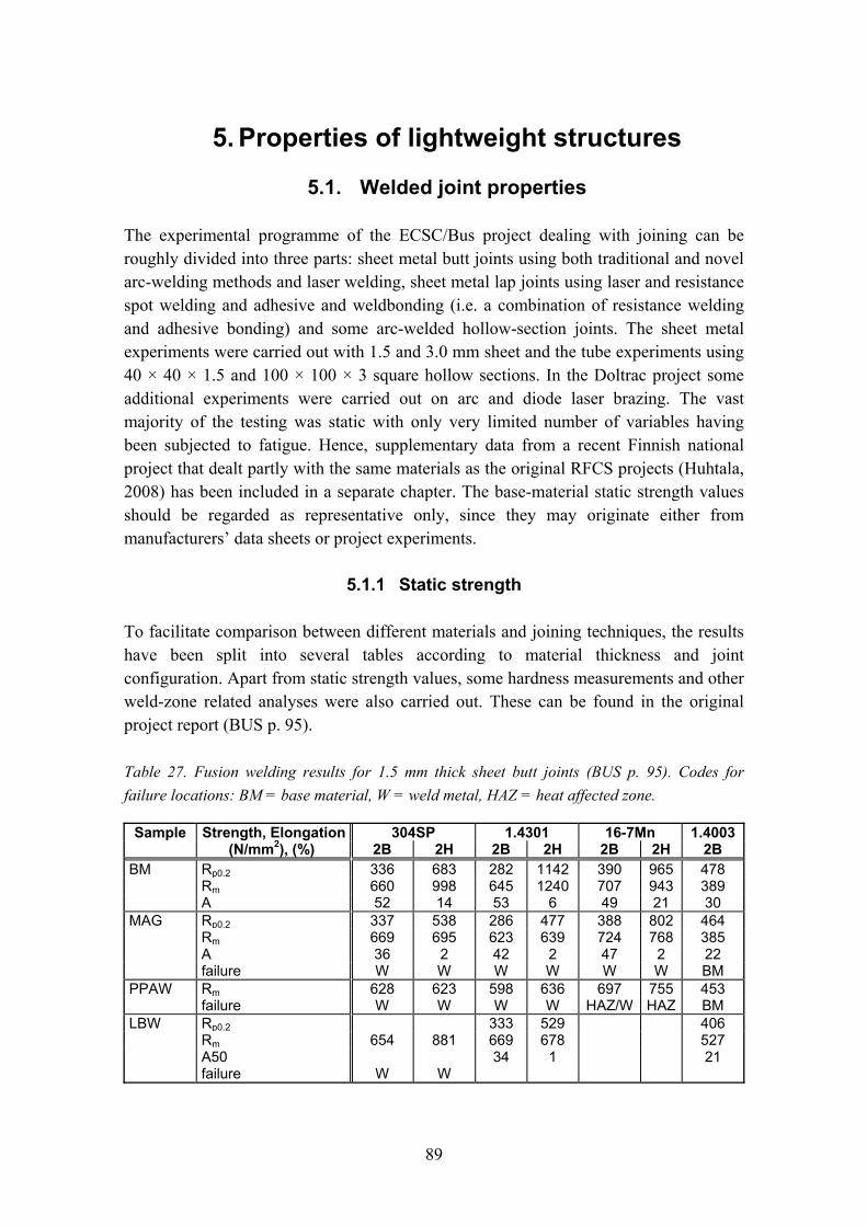
89

5. Properties of lightweight structures

5.1. Welded joint properties

The experimental programme of the ECSC/Bus project dealing with joining can be roughly divided into three parts: sheet metal butt joints using both traditional and novel arc-welding methods and laser welding, sheet metal lap joints using laser and resistance spot welding and adhesive and weldbonding (i.e. a combination of resistance welding and adhesive bonding) and some arc-welded hollow-section joints. The sheet metal experiments were carried out with 1.5 and 3.0 mm sheet and the tube experiments using 40 × 40 × 1.5 and 100 × 100 × 3 square hollow sections. In the Doltrac project some additional experiments were carried out on arc and diode laser brazing. The vast majority of the testing was static with only very limited number of variables having been subjected to fatigue. Hence, supplementary data from a recent Finnish national project that dealt partly with the same materials as the original RFCS projects (Huhtala, 2008) has been included in a separate chapter. The base-material static strength values should be regarded as representative only, since they may originate either from manufacturers’ data sheets or project experiments.

5.1.1 Static strength

To facilitate comparison between different materials and joining techniques, the results have been split into several tables according to material thickness and joint configuration. Apart from static strength values, some hardness measurements and other weld-zone related analyses were also carried out. These can be found in the original project report (BUS p. 95).

Table 27. Fusion welding results for 1.5 mm thick sheet butt joints (BUS p. 95). Codes for

failure locations: BM = base material, W = weld metal, HAZ = heat affected zone.

Sample Strength, Elongation 304SP 1.4301 16-7Mn 1.4003 (N/mm2), (%) 2B 2H 2B 2H 2B 2H 2B

BM Rp0.2 336 683 282 1142 390 965 478 Rm 660 998 645 1240 707 943 389 A 52 14 53 6 49 21 30 MAG Rp0.2 337 538 286 477 388 802 464 Rm 669 695 623 639 724 768 385 A 36 2 42 2 47 2 22 failure W W W W W W BM PPAW Rm 628 623 598 636 697 755 453 failure W W W W HAZ/W HAZ BM LBW Rp0.2 333 529 406 Rm 654 881 669 678 527 A50 34 1 21 failure W W

90

Apart from the materials included in the table, some experiments were also carried out for materials 304SP 2B and 1.4318 in C850 and C1000 temper-rolled conditions (DOLTRAC p. 99). However, because the material thickness (1.0 and 1.2 mm) and joining methods (arc and laser brazing) were different from the BUS project data, these results have not been included here but in a separate table.

According to the results in Table 27, practically full base-material strength can be obtained with MAG welding for all the base materials in 2B condition. This applies to both yield strength and tensile strength values. However, it is rather surprising that the dominant failure mode is still in the weld metal, the only exception being the ferritic 1.4003, which shows base-material failure.

The cold rolled higher-strength grades fall behind the increased base-material strength levels. The 304 sp and 16-7 Mn still retain approximately 80 % of both base-material yield strength and tensile strength but the drop is more remarkable for 1.4301: only 40 - 50 % of the base-material level is reached. However, it should be noted that the degree of strengthening due to cold forming is much higher for 1.4301, compared to other alloys. This can be seen particularly in yield strength, where cold forming has increased the base-material strength by a factor of four, whereas for other alloys the strength is increased by factors of between 2 and 2.5. The difference in tensile strength is also marked: 304SP and 16-7 Mn show a strength gain of 30 - 50 % while with 1.4301 tensile strength has almost doubled. Again, the most common failure location is the weld metal or the weld-HAZ interface. Another important feature is that elongation is lost almost completely in the cold-rolled material welds. Some drop (though much less dramatic) can also be seen in the 2B-material results.

The powder plasma arc welding experiments showed similar behaviour: for the 2B materials, strength values at or very close to the base-material tensile strengths were reached, but differences in yield strengths were greater. Only tensile strengths were determined in these tests, so the yield strengths cannot be compared to the MAG-welded results.

Laser welding is commonly regarded as one possible way to avoid the excessive drop in strength values that results from the softening of cold-rolled material. This is because the small heat input, compared to that of arc welding, results in a much narrower softened region (i.e. weld metal and HAZ). The effect is most pronounced in 304SP and 1.4003 welds. With 1.4301, the effect is less.

91

Table 28. Fusion welding results for 3.0 mm thick sheet butt joints (BUS p. 9). Codes for failure

locations: BM = base material, W = weld metal, HAZ = heat affected zone.

Sample Strength, Elongation 304SP 1.4301 16-7Mn 1.4003 (N/mm2), (%) 2B 2H 2B 2H 2B 2B

BM Rp0.2 347 831 307 590 393 429 Rm 673 977 620 795 695 557 A 51 14 56 30 51 24 MAG Rp0.2 352 514 311 456 395 335 Rm 651 726 626 664 671 452 A 33 3 33 3 26 23 failure W W W W W BM PPAW Rm 617 722 588 594 703 445 failure W W W W W BM LBW Rp0.2 333 608 392 Rm 611 892 646 776 501 A50 29 3 25 failure W/BM W

Unlike the 1.5 mm material, 16-7 Mn was only available in 2B condition for these experiments. The results are very similar to the thinner, 1.5 mm material: base-material strength is reached with all the MAG-welded materials in 2B condition and only 1.4003 shows a lower percentage (80 %) compared with previous results. Judged by percentages, the 3.0 mm cold-rolled material welds appear to retain more of the original base-material strength, but this is mainly due to the lower base-material strength values. Also, the fracture modes indicate that weld-metal strength is the governing factor – and this obviously remains the same regardless of sheet thickness. As with thinner materials, the elongation values of austenitic grades drop considerably in welded joints. This effect is most pronounced in cold-formed high-strength grades.

The PPAW welds show more or less the same strength levels as with the thinner material. In some cases, a slight tendency towards an increase in strength can be found. These remarks also apply to laser welds.

Table 29. Lap joint mechanical test results for 1.5 and 3.0 mm sheet materials (BUS p. 95).

LBW = laser welding, RSW = resistance spot welding, ADB = adhesive bonding and

WB = weldbonding.

t Sample Strength 304SP 1.4301 16-7Mn 1.4003(mm) (N/mm2) 2B 2H 2B 2H 2B 2H 2B

1.5 LBW Rp0.2 187 281 230

Rm 534 570 452 447 417

RSW Rm 152 165 202 225 248 265 97

WB Rm 400 630 375 508 430 475 383

ADB Rm 390 595 370 677 410 620 365

3.0 LBW Rp0.2 179 241 192

92

t Sample Strength 304SP 1.4301 16-7Mn 1.4003(mm) (N/mm2) 2B 2H 2B 2H 2B 2H 2B

Rm 448 491 337 346 268

RSW Rm 163 161 157 158 185 144

WB Rm 178 213 252 275 219 243

ADB Rm 287 305 263 257 346 292

The adhesive bonding was performed using a commercially available adhesive. DP490 is a two-component epoxy adhesive, produced by 3M, whose properties and applications are described in detail in the 3M publication “Solutions for Aerospace” (3M 2008).

As can be seen in Table 29, the lap joint results are mainly given as tensile strength calculated from base-material dimensions (thickness × width) only. Yield strengths were only measured from the laser-welded lap joint specimens. The use of base-material cross-section is, in practice, the only way to achieve even a rough comparison between all the the various joining methods that are feasible for thin-sheet joining in lap configuration. The resistance spot weld results suffer most from this type of comparison: there is only one spot of typically 6 mm and 8 mm in diameter in 1.5 mm and 3.0 mm sheet thickness, respectively. Hence, the load-carrying area is considerably smaller than with other methods. On the other hand, this is also a feature of RSW, and the specimen width was usually selected to represent a typical distance between two spots.

In all cases, regardless of thickness, laser welding clearly shows the highest tensile-strength values and resistance spot welding the lowest. Comparing the LBW lap joint results to butt joint results in Table 29, it can be clearly seen that they are lower, the difference being considerable. This fact emphasises the role of joint configuration in defining the strength of the structure. Direct comparisons should therefore only be made between similar configurations. Taking this approach, it is interesting to note the effect of adhesive compared to RSW. Weldbonding (a combination of adhesive bonding and resistance spot welding) increases joint strength considerably, compared to RSW without adhesive. However, the strength of weldbonded joints is always lower than that of a corresponding adhesively-bonded joint – the metallic spot weld actually decreases the joint strength of an adhesive joint, in this type of test.

Another interesting feature is that with fusion processes (i.e. laser and resistance welding) base-material strength level has only a marginal effect on joint strength. This is because in a lap joint the solidified weld pool alone carries the load and, since the strengthening effect of cold forming obviously disappears during melting and re-solidification, the weld strength remains more or less the same regardless of pre-

93

welding mechanical treatments. However, in adhesive bonding, the material is not subjected to melting or even elevated temperatures that would reverse the strengthening effect of cold forming. The effect of base-material strength can therefore also be clearly seen in adhesive joints. It is noteworthy that this effect can be seen much more clearly in the thinner 1.5 mm sheet – adhesive is the weakest link in the joint and its load-carrying capacity does not increase with greater base-material thickness. If the adhesive layer carries the same force, therefore, the strength appears to be less with thicker materials, using the current comparison approach. The behaviour of weldbonded joints is more mixed – or rather base-material dependent. The same tendencies can be seen as those that occur with adhesive bonding, but the effects are not that pronounced.

Usually, welding filler materials are selected so that the resulting joint will be as close to the properties of the base material as possible, in terms of strength and (especially for stainless steels) environmental resistance. In some cases, however, there are grounds for selecting a filler metal of a totally different type to the base material. In the case of deformation-strengthened (e.g. cold-rolled) material, one such justification is to reduce the weld heat input by using filler material with a considerably lower melting temperature, to minimise the effect of base-material softening in the vicinity of the weld and thus improve joint performance. The most typical way of reducing heat input is to use various copper-based filler metals with melting ranges several hundreds of degrees below those of steel. Basic property data and examples of such productscan be found on the bedra website (bedra 2008).

As mentioned earlier, some experiments were carried out on two brazing-based processes, namely arc and laser brazing, the latter using a high-power diode laser as the beam source. The experiments focused on two materials: 304SP in soft 2B and 1.4318 in cold-rolled C850 and C1000 conditions. It should be noted that the 304SP base-material properties differ slightly from those of previous results, because of smaller sheet thickness (1.0 and 1.2 mm). The filler metals used in these brazing experiments are introduced in Table 30 and the test results for the various base-material/filler-metal/brazing-method combinations are shown in Table 31.

Table 30. Chemical composition and key mechanical properties of the brazing filler metals used

(DOLTRAC p. 107).

Material Composition (wt %) Mechanical properties Cu Al Si Mn Ni Fe Ti others A Rm K (max) (%) (N/mm2) (J)

CuSi3 bal. - 2.9 0.9 - - - 0.5 40 350 60 CuAl5Ni2 bal. 5.0 - 0.2 2 - - 0.5 45 350 161 CuNi10Fe bal. - - 1 10.5 1.5 0.4 0.5 34 300 190

94

Table 31. Tensile strength test results for arc-brazed and laser-brazed butt joints in various

austenitic grades (DOLTRAC).

Welding Filler metal Tensile strength (N/mm2) 304SP 1.4318 2B C850 C1000

BM - 682 956 1008

arc brazing CuSi3 721 897

arc brazing CuAl5Ni2 710 783

laser brazing CuAl5Ni2 710 783

arc brazing CuNi10Fe 714 801

laser brazing CuNi10Fe 714 778

The results indicate that for 304SP, nominal tensile strength values higher than the base material can be reached. This is probably due to the test arrangements and sample geometry, etc. but it is still a very promising result. It is also worthy of note that the measured strength values remain more or less constant regardless of the filler metal or heat source used. Furthermore, the values are always higher than those for laser or MAG welding – but this may also be due to differences in experiment arrangements, since the results originate from different projects.

For the high-strength cold-rolled 1.4318 material, the brazed samples show about 10 - 20 % lower tensile strength values than the base material, as might be expected. Also, here, the differences between brazing methods or filler materials are negligible. Unfortunately, no results directly comparable to arc-welded or laser-welded joints were available for this material.

5.1.2 Fatigue and corrosion fatigue strength

Comparable fatigue and corrosion-fatigue data is available from a recent Finnish national project (Huhtala 2008). These tests were carried out using transverse test coupons of 3 mm austenitic stainless sheets, in various grades. The coupons were designed to fulfil the requirements of ASTM E 466-96, especially with regard to curvature radius. The joints were welded from one side, using matching flux-cored 308L-type filler metal for 1.4301 and 1.4318 grades. Exceptions were obviously the reference experiments made using CuSi3 solid-wire arc-brazing filler metal. Furthermore, some post-weld mechanical treatments were tested using ultrasonic peening and grit blasting.

The International Institute of Welding (IIW) Commission XIII “Fatigue of welded components and structures” (a globally recognised authority in fatigue assessment and design of welded structures) commonly uses the term FAT to describe the fatigue

95

performance of a weld-joint detail (Hobbacher 2007). To simplify, FAT is the fatigue strength at 2 million cycles. Both mean FAT50% (i.e. 50 % confidence) and characteristic FAT95% (i.e. 95 % confidence) values are used. FAT values are listed for a number of joint-type cases made of C-Mn steel or aluminium. No direct data is given for stainless steel, but C-Mn steel cases are often also used for stainless.

For the joint type tested by Huhtala (2008), IIW cases nos. 214 or 215 can be used. According to Hobbacher (2007), the characteristic FAT95% is 80 and 71 N/mm2 for cases 214 and 215 respectively. The results from Huihtala (2008) are shown in Table 32. Apart from conventional fatigue testing in air, further reference tests were carried out in both air and NaCl-environments for ferritic stainless steel 1.4003 welded with 308L filler material.

Table 32. Fatigue and corrosion-fatigue test results for 3 mm stainless steel base materials and

their butt joints (Huhtala 2008). B = arc brazing, U = ultrasonic treatment, G = grit blasting,

BM = base material.

Material & Environment

FAT Remarks

BM MAG Laser

FAT50 % FAT95 % FAT50 % FAT95 % FAT50 % FAT95 %

1.4301 air 261 200 154 105 180 108

NaCl - - 147 71 152 52

1.4318 air 311 280 137 92 - -

NaCl - - - - - -

1.4318B air - - 127 114 - - arc brazed

1.4318 air - - 131 105 - - all samples

1.4318U - - 138 98 - - UT root

1.4318G - - 124 110 - - grit blast root

1.4003 air 281 261 152 131 - -

NaCl - - 161 105 - -

It can be concluded from the results that the IIW recommendations are easily exceeded with all the tested materials, welding methods and filler materials, including the silicon bronze CuSi3 used for arc brazing. The ultrasonic or grit blasting post-weld treatments increased fatigue performance slightly but the highest FAT value for 1.4318 material was achieved with arc brazing. This was probably due to the smooth top and root reinforcement geometry typical of an arc-brazed joint, which is favourable from a fatigue point of view. A limited number of corrosion-fatigue tests were carried out for these materials but it does appear that the NaCl environment has a negative effect on fatigue strength. Nevertheless, according to these results, the joints (except perhaps the laser-welded joints) still meet the IIW requirements.

96

5.2 Sandwich panel mechanical properties

The mechanical testing programme carried out in the DOLTRAC project included both static bending tests for full-size 1250 mm × 2200 mm panels and fatigue testing of smaller panel sections, also in bending configuration. Further testing for sections was carried out in the crash test programme, described more in detail in Chapter 5.3. The panel details are collected in Table 33.

Table 33. The details of the panels manufactured and tested in the experimental programme

(DOLTRAC). The top sheet (i.e. the load-side sheet) was similar to all the other panels: 1.9 mm

thick 1.4318 in C1000 condition. dim. = RHS tube dimensions or the angle of V(f) core,

dist. = distance between individual core elements and t = sheet thickness.

Panel type Core Bottom sheet

dim. dist. mat. cond. tc mat. cond. t2

(mm) (mm) (mm)

O-1 20 × 50 84 1.4318 C850 1.0 1.4318 C1000 1.2

O-2 20 × 50 84 304sp 2B 1.0 1.4318 C1000 1.2

O-3 20 × 50 84 1.4318 C850 1.0 1.4318 C850 1.5

O-4 20 × 50 84 304sp 2B 1.0 1.4318 C850 1.5

Vf-1 60 ° 74 1.4318 C850 1.0 1.4318 C1000 1.2

Vf-2 60 ° 74 304sp 2B 1.0 1.4318 C1000 1.2

Vf-3 60 ° 74 1.4318 C850 1.0 1.4318 C850 1.5

Vf-4 60 ° 74 304sp 2B 1.0 1.4318 C850 1.5

V-1 60 ° - 304sp 2B 1.0 1.4318 C1000 1.2

The panels were designed to minimise their weight for the predetermined design-load conditions: a 480 kg/m2 = 4709 N/m2 constant load combined with a 1.5 kN point load. The maximum allowable panel displacement was set at L/300 (6.67 mm for the selected span length of 2000 mm). Apart from the verification of full-size 1250 mm × 2200 mm panel properties against the design load, the ultimate strength was measured in four-point bending. Smaller, approximately 500 mm × 1000 mm panel samples were tested in three-point bending configuration under both static and fatigue loading and 200 - 400 mm × 1800 mm sections in quasi-static and crash tests.

The fatigue programme was carried out with the worst case – maximum force amplitudes for the maximum load cycles (which would not occur in reality) – to see if the test specimens could bear these loads. The selected case was based on a typical equipment box of ~ 2.5 tons, mounted with eight brackets, inducing a force of 3000 N per bracket (i.e. a 3 kN point load) on a 100 × 100 mm2 square representing the underfloor equipment-box bracket. This static load was superposed by ± 20 % dynamic loads, leading to R = 0.66 with an upper amplitude of 3600 N and a lower amplitude of

97

2400 N. Thus, the specified fatigue load was 3000 N ± 600 N applied to an area of 100 × 100 mm2 for 107 cycles at a maximum frequency of 100 Hz.

5.2.1 Four-point bend testing of full-size panels

The bending tests were carried out in a customisable load frame, using two separate loading cylinders and displacement control. The forces were measured directly from the hydraulic cylinders and the displacements from both the top and bottom panel surfaces. The bending tests were carried out using displacement control at a speed of ~ 3 mm/min. Details of the test arrangements can be found in Figure 59.

Figure 59. Details of panels in the four-point bending test, showing a) top-sheet wrinkling

under compressive load and b) failure caused by local buckling of the core element.

Altogether, 18 full-size panels were tested by four-point bending. Apart from the maximum loading force and the corresponding displacements, an effort was also made to evaluate the yielding behaviour of the panels. Determining a reliable and common yield criterion for all the panels proved too difficult, however, mainly because the scatter originating from the distortion of the panels after welding was too great. Instead, the slope of the elastic region of each force-displacement curve was defined, to gain at least a rough estimate of the elastic behaviour of various panel types under loading.

An effort was made to evaluate the elastic behaviour of the panels, by determining the slope of the load-displacement curve of each panel at the elastic region. Both panel types show – within reasonable scatter – approximately the same slope, which depends mainly on the thickness of the bottom sheet. Increasing the thickness from 1.2 mm to 1.5 mm results in a 15 - 20 % higher slope value. It is also noteworthy that the scatter is less for the thicker, bottom-sheet panels. In the theoretical panel-optimisation calculations, the decrease in displacement caused by the change of bottom-sheet thickness from 1.0 mm to 1.5 mm is 17.5 % and 18.4 % respectively for the O- and Vf-panels (i.e. comparable to the experimental results).

98

Figure 60 shows a representative load-displacement curve for each panel type and variant. As a conclusion, it can be said that when the panel surface-sheet thicknesses are the same, there are no significant differences in the suitability of different panel types or manufacturing routes, from a load-bearing point of view. The differences become evident at loads and resulting displacements that are far beyond acceptable for any floor structure. However, the improved maximum load-bearing capacity can be utilised in exceptional impact-load situations, such as crash or collision. Choice between panel details therefore has to be based on weighing up other factors, such as: the advantages of using standard RHS tube cores rather than tailored sheet Vf profiles against the punishment in panel weight, or the smooth and intact sheet surfaces available with adhesive bonding against increased panel-assembly time and the uncertain long-term durability of adhesive joints.

Figure 60. The four-point bending test load – displacement curves and maximum load figures of

different types of panels with a 1.5 mm 1.4318 C850 bottom sheet and continuous laser welds.

5.2.2 Three-point bend testing of panel sections

The three-point bending test was originally designed for fatigue testing panel sections, it having been foreseen that performing fatigue tests for full-size panels would be too resource-intensive.It was therefore decided that the fatigue-testing programme would be carried out with panel sections suitable for testing in universal testing machines, instead of tailored arrangements required for full-size panels. Originally, sections cut in both longitudinal and transverse directions were to be tested. Later, it was decided that a

174

157106

175

0

50

100

150

200

250

0 20 40 60 80 100 120

Displacement (mm)

Str

ess

(kN

/m2 )

Vf-3-3 (foam)

Vf-3-4

Vf-4-0 (adhesive)

O-3-2

99

limited number of static bending tests until fracture would also be performed with this arrangement, before comparing the bending behaviour of all three panel types.

The dimensions of the panel sections were based on the available universal testing load frames. The 21”, 535 mm spacing between the load-frame columns sets the maximum specimen width. On the other hand, the number of longitudinal core elements has to be odd, in order to introduce the loading tool on a core rather than on the unsupported sheet surface between them. This resulted in a section width of 500 mm, accommodating five-hollow-section and three Vf-core elements. Correspondingly, the span length was primarily determined by the odd number of transverse core elements between the supports, resulting in a span of 800 mm.

Figure 61 shows the longitudinal static three-point bending test results of different panel types. It can be clearly seen that the V-core panel is the stiffest panel in the early stages of the elastic region, which is the most important area in terms of practical load-bearing applications. The force required to achieve an L/300 (i.e. 2.67 mm) displacement is about 50 % higher than for the O- or Vf-type panels and the slope is about 20 % higher, even if the bottom sheet is thinner.

Figure 61. Load-displacement curves and panel weights of three different panel types.

As mentioned earlier, the defined fatigue-loading situation originates from the attachment of an underfloor equipment box. Converted to panel-section testing, this

262 kN/m2 / 36.4 kg/m2

133 kN/m2 / 33.4 kg/m2

226 kN/m2 / 36.6 kg/m2

0

50

100

150

200

250

300

0 5 10 15 20 25 30

Displacement (mm)

Str

es

s (k

N/m

2 )

O-3-0

Vf-4-3

V-core

100

means a goal of 107 cycles fatigue life under a 3000 N ± 600 N (7.5 kN/m2 ± 1.5 kN/m2) load (R = 0.66) applied to an area of 100 × 100 mm2.

Table 34. Fatigue testing results of panel sections. For panel details see Table33.

Panel Core direction σ f N ∆s

(kN/m2) (Hz) (mm)

O-2-3 transverse 7.5 ± 1.5 2 1 352 000 6.13

O-2-3 longitudinal 7.5 ± 1.5 20 30 17 022 750 0.19

O-4-2 longitudinal 63 ± 13 10 1 538 000 1.31

O-4-3A longitudinal 100 ± 20 5 1 724 400 2.00

O-4-3B longitudinal 188 ± 38 5 12 140 4.00

V-2-1 longitudinal 7.5 ± 1.5 30 40 10 506 280 0.17

Vf-4-3 transverse 7.5 ± 1.5 4 2 388 800 3.14

Vf-4-3 longitudinal 7.5 ± 1.5 30 15 568 000 0.18

Vf-4-2 longitudinal 63 ± 13 8 5 1 580 500 1.74

Vf-4-3B longitudinal 75 ± 15 5 1 767 800 2.10

Vf-4-2B longitudinal 100 ± 20 5 166 060 2.60

As can be seen in the fatigue results in Table 28, all the panel types with longitudinal cores survived the fatigue-loading criteria. Because only one V-type panel was available, this verification test was the only one performed for this panel type. For other panels, higher loads were also used. The O- and Vf-panel results at higher loads show that a fatigue life of 106 cycles is realistic for them, in practice, under 25 ± 5 kN (63 ± 13 kN/m2) loading. Above this load level, the initial core buckling confuses the situation, but at least the O-core panels show potential for even higher loads. Despite the promising results, one should be cautious about drawing further conclusions regarding the fatigue properties of these panels, because of the extremely limited number of specimens tested.

5.2.3 Summary and conclusions

It can be concluded that all the panel types easily meet the set requirements for the static (i.e. design-loading) and fatigue-loading situations. However, the panel optimisation calculations gave excessive displacement values compared to the experimental calculations. In practice, reaching L/300 displacement required approximately 3 to 4 times the design load. In other words, there remains potential for further weight saving in these panels.

When the O- or Vf-panel surface-sheet thickness and the total panel thickness are the same, there are no significant differences in the suitability of different panel types,

101

material strengths or manufacturing routes, from a load-bearing point of view. The practical structural properties are stiffness-dependant (i.e. geometry-dependent). The differences in panel type (O- or Vf-type), material strength (e.g. a high-strength grade) or assembly method (e.g. discontinuous welds, adhesive bonding) only become evident at loads and resulting displacements that are far beyond acceptable for any floor structure – apart from exceptional impact-load situations, such as crash or collision.

Thus, choice between panel details has to be based on weighing up other factors, such as: the advantages of using standard RHS tube cores rather than tailored sheet Vf-profiles against the punishment in panel weight, or the smooth and intact sheet surfaces attainable by adhesive bonding against increased panel-assembly time, or the improved stiffness characteristics of a V-type panel in bending against extensive difficulties in panel manufacture and assembly. In static longitudinal tests, global buckling is the major failure mode, while in the crash tests local buckling at the end of the panels is the major failure mode, leaving the middle of the panel almost without significant, irreversible (lateral) deformation. The lack of lateral deformation and the fact that crumpling is only at the ends leaves the passenger region quite unharmed. This is the most favourable condition that can be desired for a passenger compartment, in terms of crashworthiness.

In transverse tests, the buckling mode for both static and crash test show more similar features. The panel showed more widespread plastic deformation, clearly visible in the large lateral deformation. These large lateral displacements would be transmitted to the passengers in this region, giving them the first primary shock load. Also, the amount of elastic energy stored in a sideways collision is considerable. Beside the large lateral displacements in the panel, elastic deformation can be released from the structure after the initial impact, resulting in a secondary shock load inflicted on the passenger in the crumpled region.

The maximum energy absorption could not be established in the crash test facility. Both mass and velocity were limited, but it is plausible that a longitudinal panel can absorb significantly more energy than could be tested for. In general, all panels performed quite similarly in the longitudinal tests. In the transverse tests, the O-core panels dissipate about 25 % less energy compared to the Vf-core.

102

5.3 Lightweight structure crash properties

The crash properties of various lightweight stainless steel structures were tested extensively in both the BUS and DOLTRAC projects. A summary of the types of tests used and the results achieved is given in the following chapters.

5.3.1 Axial impact tests

Square stainless steel hollow sections of 40 × 40 × 1.5 mm were tested axially on a horizontal crash test rig. The sections were tested at an energy level of 7.5 kJ, achieved by a virtual mass of 218 kg impacting the sections at a speed of 8.7 m/s. The sections were all triggered by expansion of the tube end. The comparison between different materials was made using the concept of “mean load”, determined from the load-displacement curve. This measurement is an average value for the load during the entire impact, used here to compare the sections’ structural performance. A higher mean load means higher energy absorption per length unit during side impact and hence better structural performance. A summary of the axial crash test result is given in Table 35. Details of the experimental arrangements, together with more exhaustive test results, can be found in BUS (p. 159).

Table 35. Mean axial crash test results for stainless steel hollow sections (BUS p.161).

Mean axial crash results Material grade

1.4301 304SP 1.4003

Mean peak load (kN) 32.52 42.08 29.80

Mean load (kN) 13.50 16.57 10.26

Mean crash speed (m/s) 8.69 8.70 8.76

Mean crash length (m) 0.14 0.11 0.18

Ranking the materials in the axial impact test according to performance, starting with the highest load and lowest crash length, the order is 304SP (austenitic), 1.4301 (austenitic) and 1.4003 (ferritic) – i.e. the austenitic hollow sections show better resistance against axial crash than the ferritic hollow section. All the materials showed stable collapse during axial impact.

5.3.2 Side impact tests

As in the axial crash tests, 40 × 40 × 1.5 mm square hollow sections were tested in a horizontal crash test rig fitted with a 3-point bending tool. The sections were tested at an energy input level of 1000 J, achieved with a crash mass of 229 kg impacting the

103

section at a velocity of 3.0 m/s. Figure 62 shows a sketch of the experimental arrangement and Table 36 summarises the test results.

Figure 62. Diagram of the side-impact test arrangement (BUS p. 162).

Table 36. Mean side-impact test results of stainless steel hollow sections (BUS p. 163).

Mean side impact results Materials grade 1.4301 304SP 1.4003

Mean peak load (kN) 5.60 7.20 4.89 Mean load (kN) 2.01 3.19 1.99 Mean crash speed (m/s) 3.02 2.97 2.96

Ranking the materials in the axial impact test according to performance, starting with the highest load and lowest crash length, the order is 304SP (austenitic), 1.4301 (austenitic) and 1.4003 (ferritic) – i.e. the austenitic hollow sections show better resistance against axial crash than the ferritic hollow section. All the specimens showed global buckling during side impact.

5.3.3 Tubular frame crash tests

Typical structural subframe mock-ups of a bus structure were tested for crash performance in the BUS project, Figure 63. The tested frames consisted of square hollow sections of 40 × 40 × 1.5 mm, in stainless steel grades 1.4301 (austenitic), 1.4003 (ferritic), 304 SP (austenitic) and 16-7 Mn (austenitic), and galvanised carbon steel grade St37 for reference. All frames were powder plasma arc welded (PPAW).

The welded frames were crash tested on a horizontal crash test rig at an energy level of 5.1 kJ, achieved by a mass of 312 kg impacting the sections at a speed of 5.7 m/s. A hollow cylinder with a diameter of 230 mm was mounted, for a bumper, at the front

Test sample

Crash mass with

indentor

Velocity50 mm diameter

340 mm

Displacement

top face

Displacement

bottom face

104

edge of the crash mass. The welded frame was hung on a mounting frame and clamped at two points on the test rig (Figure 63). The frames were tested at –20 °C and +5 °C.

Figure 63. Frame before (left) and after (right) impact test (BUS p.169).

The frame crash test arrangements and quantitative results are given in detail in BUS (p. 169) so only a summary is given here (Figure 64, Figure 65 and Table 37). As a general summary, it can be said that crash resistance as defined by the deflection of frame members is best with the austenitic grades. Ferritic grade 1.4003 also performs well at temperatures above zero, but the crash resistance degrades at –20 °C, to below that of 1.4301. The reference material, mild galvanised steel St37, shows the most modest performance at all frame locations and temperatures. This is largely due to its low initial strength level combined with a lack of strain-hardening capability.

Figure 64. The square hollow-section frame used for crash tests. Left: main dimensions. Right:

tube codes (BUS p. 173). Note the different angles of view.

1000 mm

550 mm

695

mm

A

C

EBD

H

F

G

M

I

L K

J

1000 mm

550 mm

695

mm

A

C

EBD

H

F

G

M

I

L K

J

105

Figure 65. (a) Deflection of buckled members A, C and E, (b) deflection of side members J, K, L

and M defined as deflection = b – a, (c) height of deformed cross-section ends Bfront and Dfront.

Table 37. Ranking of the test frames: crash performance with respect to different mean

dimensional changes as described in Figure 65, starting with the lowest (i.e. best) value (BUS p.

174). The frame member codes are shown in Figure 64.

Rank Deflection Deflection of side members

Height of deformed cross-section

Mean total crack length in

A, C, E J, M, K, L B, D weld lines +5 °C -20 °C +5 °C -20 °C +5 °C -20 °C +5 °C -20 °C

1 304SP 304SP 304SP 304SP 304SP 304SP 1.4301 1.4003 2 16-7Mn 16-7Mn 16-7Mn 16-7Mn 16-7Mn 1.4301 1.4003 1.4301 3 1.4003 1.4301 1.4003 1.4301 1.4003 16-7Mn 16-7Mn 304SP 4 1.4301 1.4003 1.4301 1.4003 1.4301 1.4003 304SP 16-7Mn 5 St37 St37 St37 St37 St37 St37 St37 St37

The total crack length in the welding lines is almost equal (±2 mm) for 1.4301, 1.4003 and St37 at both +5 °C and –20 °C. However, the crack length for 16-7Mn and 304SP decreases drastically with temperature. Total crack length decreases from 40 mm to 15 mm for both materials at temperatures of +5 and –20 °C, respectively.

Weld-line cracking occurred at the nodes where the frame members are welded together. In all frames, deformation at member-ends Mtop and Jtop is absorbed by deformation of the open tube-section ends Bfront and Dfront. In the left and right nodes of member A, energy was absorbed by the cross-sectional deformation of tubes B and D.

5.3.4 Panel compression and crash testing

Quasi-static compression tests were carried out on panel sections, to determine buckling strength and buckling mode, as background information for dynamic crash of the panels. In this case, panel deformation consists of two parts: below the buckling load, very large forces but small axial displacements result in low elastic-energy absorbing capacity. Here, the only relevant parameters are the modulus of elasticity, moment of inertia of the cross-section and panel length. After the buckling load (post-buckling), the

a

b

a

b

(a) (b) (c)

a

b

a

b

(a) (b) (c)

106

panel will develop plastic deformation and energy is absorbed in the panel. Here, the relevant parameters are yield strength, hardening behaviour, strain-rate sensitivity, ductility and buckling modes.

The static tests were limited to O-core and Vf-core, simply because there was a limited number of valid V-core panels available for both the static and dynamic tests. The tests were performed in a pseudo simply-supported manner and under quasi-static testing conditions. For comparison purposes, normalised failure energies (i.e. energy divided by panel-section width) were used. From the start of the test, the welds audibly cracked on both O- and Vf-core panels and maximum normalised energies of 2.5 and 1.9 J/mm respectively were measured before buckling (Figure 66a). Theoretically, the diference should have been about one third of this for O-panels and the maximum loads should have been double those measured for both types. In the transverse tests, the maximum force is only a fraction of the longitudinal tests (Figure 66a) and the Vf-panel shows about double the normalised buckling energy to O, as expected.

(a) (b)

Figure 66. (a) Quasi-static panel compression test results: L = longitudinal and T = transverse;

(b) panel transverse crash test results. Normalised energies are used because of the varying

panel section widths.

The rig used for the crash tests had a 267 kg ram, launched by means of a pneumatic cylinder up to maximum of 9.5 m/s, corresponding to 11 kJ kinetic energy in the ram. The ram slid along the rails on sliding pads and speed was measured just before impact. The panel was clamped in a pseudo simple-supported way. Because all panels absorbed the full amount of energy applied to them in the longitudinal tests, only minimum performance values can be given: at least 55, 40 and 60 J/mm of energy can be dissipated by O, Vf and V panels of this type, respectively. Figure 67 shows some longitudinally tested panels.

2.5

1.9

0.16

0.30

0.0

0.5

1.0

1.5

2.0

2.5

3.0

O-core L Vf-core L O-core T Vf-core T

Panel type and direction

Em

ax/

w, l

on

git

ud

ina

l (J/

mm

)

15.4

20.5

0

5

10

15

20

25

30

O-core Vf-core

Panel typeE

ma

x/w

(J/

mm

)

107

Figure 67. Panel sections after longitudinal crash tests.

In the results for the transverse tests (Figure 68) there is a significant difference between O and Vf-core panels tested at the same speed. This is well in line with quasi-static tests and can be explained by the contribution of the cores to energy absorption. Vf cores allow more elastic deformation and thus convert kinetic energy more effectively into elastic deformation – indicated by ram bouncing – whereas O-cores guide the energy into plastic deformation in the surface sheets. A significant difference between buckling modes was detected: in the static test the global buckling mode was mainly activated while in the crash test local buckling was predominantly present at the panel ends.

(a) (b)

Figure 68. Panel sections after transverse crash tests: (a) O core = rectangular hollow section

type and (b) Vf core = sheet profile type (DOLTRAC p.187).

109

6. Life cycle issues

The transporting of goods by road plays a significant role in our society and has increased significantly in the last 20 years. Without major new measures, heavy goods vehicle traffic in the European Union (EU) is predicted to increase further, to almost 50% above its 1998 level, by 2010 (European Commission 2001). Road transport is still a major source of air pollution, although technical advances have significantly improved the environmental performance of engines and road traffic. Vehicle engines burn fossil fuels containing carbon and are thus a source of carbon dioxide (CO2) emissions. The OECD has predicted that the share of CO2 (the main anthropogenic greenhouse gas) emissions from road traffic to total greenhouse-gas emissions will increase from 20 % of the total in 1995 to 30 % by 2020 (UNEP 2002).

6.1. Effect of vehicle weight on life cycle cost

Vehicle weight has a significant effect on fuel consumption. A clear trend can be seen in Figure 69, which shows the combined consumption and weight of the 10 most popular new passenger cars from every segment in German market.

Figure 69. Combined consumption and weight of the 10 most popular new passenger cars, from

every segment, in Germany (KBA 2008).

A recent Finnish study suggests that vehicle weight reduction and the development of aerodynamic performance could lower airborne emissions of heavy road traffic by 30 %

Fuel consumption of new passenger cars(Germany 2006, KBA)

3

5

7

9

11

13

15

500 700 900 1100 1300 1500 1700 1900 2100 2300 2500 2700

Weight (kg)

Co

nsu

mp

tio

n (

litr

es/1

00 k

m)

Petrol Diesel Trends

110

(Nylund 2006). Reducing empty weight could directly increase the payload weight fraction in commercial road traffic, which would improve both the economic and environmental performance of freight transport.

Figure 70 shows how vehicle weight affects the fuel consumption of heavy vehicles.

Figure 70. Fuel consumption and weight of heavy road traffic (Nylund 2006, Mäkelä 2008).

While steels have long been the dominant structural materials for the transportation industry, over the years, the industry has sought alternative means and materials, to improve the performance of vehicles. Structural solutions using different materials vary in their weight, material production and recycling. It is therefore clear that a comprehensive life cycle perspective is needed when considering the environmental performance of vehicles. Long product life cycle, in terms of years and kilometres, differentiates commercial vehicles from private cars. Heavy transportation therefore requires individual analyses that take all life cycle stages into account, from raw-material production to the end of life.

As one of the major material producers, the steel industry is committed to the concept of sustainable development and is keen to improve the environmental performance of its products. To provide the necessary product information to interested parties, the European steel industry has contributed to an Integrated Product Policy (IPP), in response to the European Commission’s communication on IPP released in June 2003. The aim of IPP is to identify and minimise environmental impacts caused by products

Fuel consumption of heavy road transportation(VTT)

0

10

20

30

40

50

60

0 10000 20000 30000 40000 50000 60000 70000

Weight (kg)

Fu

el c

on

sum

pti

on

(li

tres

/100

km

)

City bus

60t truck

42t semitrailer

111

and services, occurring throughout the phases of their life cycle, whether from manufacture, use or disposal (Eurofer 2008).

6.2. Environmental effects of bus-frame materials

Buses and coaches are normally divided into city, inter-city (long distance). Bus types differ in drive cycle and construction. Inter-city buses and coaches are used on longer routes with relatively few stops, while city buses stop and accelerate frequently because of city traffic and passenger pickups.

Weight reduction improves fuel economy and reduces materials consumption. These improvements produce lower emissions and reduce the amount of materials to be produced and recycled. Design optimization, innovative constructions and the use of high-strength materials are all important ways to reduce weight. Reducing vehicle weight affects the costs, environmental performance and safety performance of a vehicle. Overall, fuel consumption depends on powertrain efficiency, climbing resistance, rolling resistance, acceleration resistance, aerodynamic drag and vehicle mass.

Vehicle mass reduction has complex effects on fuel consumption, since weight reduction in one part affects the design and weight of the other parts. Comparing individual parts of large systems gives only some indication of actual effects. The effects of primary weight reduction extend to other components as secondary weight reductions, which further lower overall weight. Fuel consumption can also be lowered by a modified transmission ratio and a smaller engine. If curb weight is lowered, it is possible to achieve comparable driving performance with a different transmission and less power, which also lowers fuel consumption (Eberle et al. 1998, Nylund 2006). Nominal diesel oil consumption of a city bus varies from 42 to 53 litres per 100 km, depending on payload (Mäkelä 2008). A Finnish study states that a vehicle weight saving of 1000 kg reduces fuel consumption of a city bus by 2 litres per 100 km (Nylund 2006).

The airborne combustion emissions from a diesel engine of a bus in short-distance city traffic shown in Table 38 are average unit emissions from different EURO-level buses measured and calculated in the Finnish studies (Mäkelä 2008). Use-phase emissions consist of emissions from fuel production and tailpipe emissions from fuel combustion. The diesel-combustion emissions in the Table are quite similar to the values used in the previous bus study (BUS) but more recent. They give a good estimation of tailpipe emissions.

112

Table 38. Airborne emissions from the diesel engine of a bus in short-distance (city) traffic

(Mäkelä 2008). Cons. = fuel consumption.

Emission class

CO NOx PM CH4 NMHC N2O SO2 CO2 Cons.

(g/km) (g/km) (g/km) (g/km) (g/km) (g/km) (g/km) (g/km) (g/km)

EURO 3 0.6 9.7 0.21 0.03 0.10 0.035 0.0042 1340 423

EURO 4 0.5 6.8 0.04 0.03 0.06 0.035 0.0042 1340 423

EURO 5 0.5 3.9 0.04 0.03 0.06 0.035 0.0042 1340 423

The industry associations of steel and stainless steel producers have collected materials-production LCI data. These inventories are available for use in Life Cycle Assessment (LCA) studies. They all give a “cradle-to-gate” point of view, including efficient recycling. The recycling ratio of ferrous metals for European end-of-life vehicles is between 98 % and 99 %, while 1-2 % goes to waste as metal landfill (Beck 2004, Ridge 1998). Bus frames are fairly easy to dismantle and recycle.

6.3. Life cycle cost evaluation of bus-frame materials

The life cycle cost of a bus frame includes the materials and manufacturing costs of the frame and the operating costs. Bus-frame structures are manufactured using welded hollow sections and sheets. The difference between carbon steel and stainless steel frames is that a carbon steel frame must be completely painted, to protect the welded hollow sections from corrosion. Long frames need a large dip-painting tank, which implies a corresponding capital investment. The chromium content of stainless steels, however, ensures adequate corrosion protection and removes the need to paint frames. This gives stainless steel an advantage in terms of manufacturing costs.

The operating costs of a bus frame are largely determined by fuel consumption and, therefore, frame weight. Lower operating costs can therefore reduce the life cycle cost of a lighter bus. Figure 71 shows how significant fuel costs are, compared to materials costs. This is why the curb weight of a bus is important in the quest for low life cycle cost with reduced operating costs.

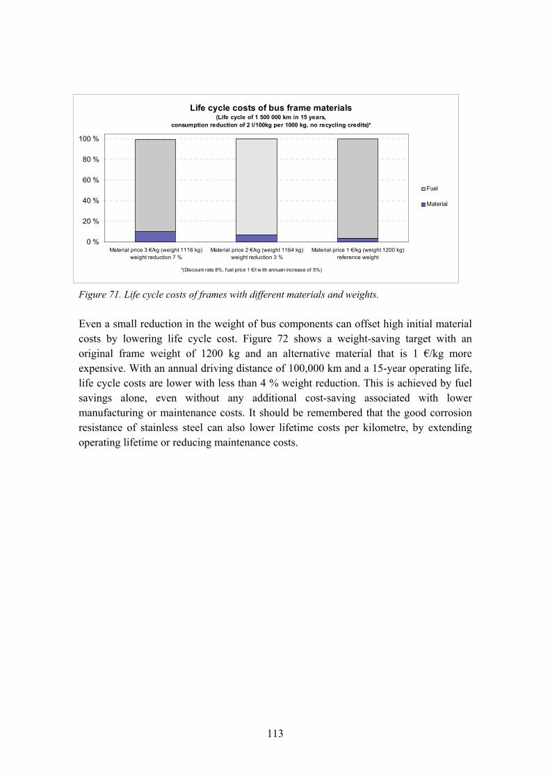
113

Figure 71. Life cycle costs of frames with different materials and weights.

Even a small reduction in the weight of bus components can offset high initial material costs by lowering life cycle cost. Figure 72 shows a weight-saving target with an original frame weight of 1200 kg and an alternative material that is 1 €/kg more expensive. With an annual driving distance of 100,000 km and a 15-year operating life, life cycle costs are lower with less than 4 % weight reduction. This is achieved by fuel savings alone, even without any additional cost-saving associated with lower manufacturing or maintenance costs. It should be remembered that the good corrosion resistance of stainless steel can also lower lifetime costs per kilometre, by extending operating lifetime or reducing maintenance costs.

Life cycle costs of bus frame materials(Life cycle of 1 500 000 km in 15 years,

consumption reduction of 2 l/100kg per 1000 kg, no recycling credits)*

0 %

20 %

40 %

60 %

80 %

100 %

Material price 3 €/kg (weight 1116 kg)weight reduction 7 %

Material price 2 €/kg (weight 1164 kg)weight reduction 3 %

Material price 1 €/kg (weight 1200 kg)reference weight

Fuel

Material

*(Discount rate 8%, fuel price 1 €/l w ith annuan increase of 5%)

114

Figure 72. Proportional weight savings that offset a 1 € per kg higher material price in the life

cycle fuel cost of bus components.

These calculations demonstrate the importance of vehicle weight in bus transportation. The same principle also applies to other road transport vehicles. The diesel consumption of trucks and other commercial vehicles also depends on the payload and, once again, weight savings can be used to increase payload or lower fuel consumption. In the case of heavy trucks, a vehicle weight saving of 1000 kg reduces fuel consumption by approximately 1 litre per 100 kilometres (Nylund 2006). This can be significant, because of ever longer driving distances and the continued increase in freight transport by road. In typical service conditions, the potentially higher initial cost of using stainless steel, compared with carbon steel, is largely offset by the effect of the resulting weight saving on fuel consumption.

Although they go beyond the scope of this study, the following factors, which have a further influence on life cycle cost, should be addressed:

• In contrast to carbon steel, where metallic and organic coatings and painting provide corrosion protection, with stainless steel, these essentially have only a decorative function. The number of layers can therefore be reduced and the overall structure of the coating simplified. Because of stainless steel’s intrinsic corrosion resistance, corrosion-related repair costs can be expected to be lower.

• Accidental damage or wear and tear that locally weaken or remove the corrosion protection on carbon steel have no effect of the intrinsic corrosion resistance of stainless steel. Even if damage should lead to localised discolouration

Weight reduction that compensates high material costs (bus frames)(Fuel consuption 2 l/100 km per 1000 kg, no recycling credits)*

0 %

3 %

5 %

8 %

10 %

6 years 10 years 15 years 20 years

Operating lifetime

Wei

gh

t re

du

ctio

n t

arg

et

75 000 km/year 100 000 km/year

*(Discount rate 8%, fuel price 1.2 €/l w ith annual increase of 5%, difference in material cost is 1 €/kg )

115

(especially in the case of lower-alloyed ferritic stainless steels), this will neither spread into neighbouring areas nor lead to serious corrosion.

• Because of the outstanding weldability of stainless steels (especially austenitic grades), the reparability of stainless steel structures is exceptionally good.

• As the material contains valuable alloying elements such as chromium and nickel, the scrap value of buses containing stainless steel at the end of their service life is higher than that of other designs.

To quantify all these effects, simplified Life Cycle Costing software is available, allowing designers and operators to make comparative calculations based on their own cost figures (Euro Inox 2002).

6.4. Summary

Weight reduction and overall vehicle weight plays a vital role in the environmental performance of a city bus. Bus-frame weight reduction makes it possible to either downgrade power-source requirements or increase payload capacity. Both options increase the effectiveness of bus transport. Materials selection and bus-frame weight reduction are important and have positive environmental effects. Life cycle calculations show conclusively that reducing the weight of a vehicle lowers fuel consumption and can fully compensate for an initially higher material cost.

117

Acknowledgements

The following organisations provided financial support for the publication of this handbook. Their assistance is gratefully acknowledged.

• Research Fund for Coal and Steel (RFCS), (formerly European Coal and Steel Community (ECSC)), that financed both the two underlying research projects and the dissemination project for the preparation of this handbook, under the following contracts: STAINLESS STEEL BUS, contract 7210-PR-176; DOLTRAC, contract 7210-PR-363; and INSAPTRANS, contract RFS2-CT-2007-00025.

• The European stainless steel producers and other organisations that have contributed to this handbook through participation in all three above-mentioned projects.

A project steering committee including representatives from each partner and sub-contractor oversaw the project work. The following were members of the project steering group (PSG) and/or contributed to preparation of the manuscript:

Tero Taulavuori Outokumpu Stainless Oy (PSG chairman)

Nico de Wispelaere OCAS N.V.

Leopoldo Rizzo Centro Sviluppo Materiali (CSM) S.p.A.

Thomas Pauly, Alenka Kosmač

Euro Inox ASBL

Rafael Sánchez Acerinox S.A.

Raf Thys, Roeland Vliegen, Benoît van Hecke

ArcelorMittal Stainless Belgium N.V.

Hannu Hänninen, Joona Säynevirta

Helsinki University of Technology

Mika Sirén, Pekka Pohjanne, Hannele Tonteri, Tiina Ala-Outinen

VTT Technical Research Centre of Finland (coordinator, PSG secretary)

The technical data and design recommendations presented in this document are based on the best knowledge available at the time of publication. However, no responsibility of any kind for injury, death, loss, damage or delay, however caused, resulting from the use of the recommendations, can be accepted by the project partners or others associated with its preparation.

119

References

Ala-Outinen, T. 1996. Fire resistance of austenitic stainless steels Polarit 725 (EN 1.4301) and Polarit 761 (EN 1.4571). Espoo: Technical Research Centre of Finland. 33 p. + app. 30 p. (VTT Research Notes 1760).

Ala-Outinen, T.,Oksanen, T. 1997. Stainless steel compression members exposed to fire. Espoo: Technical Research Centre of Finland. 41 p. + app. 17 p. (VTT Research Notes 1864).

Ala-Outinen, T., Viherma, R., Nilimaa, H. 2003. Isothermal material tests of cold worked Stainless Steels. Stainless Steel in Structures. International Experts Seminar. Ascot, UK, 20 May, 2003. The Steel Constructions Institute. Ascot, Berkshire, SL5 7QN, UK (2003), pp. 21-26.

Alenius, M., Talonen, J., Hänninen, H. and Vilpas, M. 2002. Ruostumattomat kotelo- ja kennolevyt kuljetusvälineissä (Stainless box and sandwich panels in transport equipment). Espoo: VTT Research report VAL22-023283. 46 p. + app. (in Finnish).

Aluminium Taschenbuch, 14. Auflage (3., datenaktualiserter Druck 1988). 1988. Düsseldorf: Aluminium-Verlag. ISBN 3-87017-169-3. 1094 p. p. 65.

Arnold, N., Gümpel, P. & Heitz, T.W. 1999. Chloride induced corrosion on stainless steels at indoor swimming pools atmospheres. Part 2: influence of a real indoor swimming pool atmosphere. Materials and Corrosion, 1999, vol. 50, p. 140-145.

ASSDA (Australian Stainless Steel Development Association). 1996. Corrosion resistance in marine atmospheres. Australian Stainless Magazine, No. 6, 1996.

ASSDA (Australian Stainless Steel Development Association). 2008. Corrosion Resistance in Marine Environments. URL: http://www.assda.asn.au/index.php?option=com_content&task=view&id=170&Itemid=135 (referred to in June 2008).

Australian Stainless. 2001. Australia’s First Stainless Steel Bus, Australian Stainless 18 (2001).

Atlas Specialty Metals. 2008. Major coal wagon steel supply contract awarded to Atlas by Queensland Rail. URL: http://www.atlasmetals.com.au/news.asp?NID=69 (referred to in August 2008).

120

Baddoo, N. 2007. Stainless Steel in Construction: A review of research, applications, challenges and opportunities, Stainless Steel in Structures: Third International Experts Seminar, The Steel Construction Institute, Ascot, UK, 2007.

Baddoo, N.A., Burgan, B.A. 2008. A fire engineering approach to the design of stainless steel structural systems. In: Proceedings of the 6th European Stainless Steel Congress, Helsinki, 2008. pp.381–386.

Baroux, B. 1995. Further insights on the pitting corrosion of stainless steels. In: Marcus P, Oudar J, editors. Corrosion mechanisms in theory and practice. New York: Marcel Dekker, 1995.

Beck, M. 2004. Cracking the End-of-vehicle Conundrum, Recycling International, April 2004, pp. 20-25.

bedra®. 2008. Product overview. URL: http://www.berkenhoff.de/index.php (referred to on 23.4.2008).

Bombardier Transportation. 2007. URL: http://www.bombardier.com.

Centro Inox / De Simon. 2005. URL: http://www.desimon.it.

Charles, J. 2005. The new 200-series: An alternative answer to Ni surcharge? Dream or nightmare? In: Proceedings of the 5th European Stainless Steel Science and Market Congress, Seville, Spain, 2005. pp.19–27.

CIDECT. 1996. Project 5AQ/2.

Cochrane, D. 2005. Guide to stainless steel finishes. Building Series, Volume 1. Brussels: Euro Inox. ISBN 2-87997-173-X. 21 p. Also available as CD-ROM (2007) and for download at URL: http://www.euro-inox.org/

Connor, L. P. (ed.). 1989. Welding Handbook, Vol. 1 Welding technology. Eighth edition, second printing. 1989, American Welding Society (AWS), Miami, Fl. ISBN 0-87171-281-4. p. 16.

Council of Europe. 2001. Technical document: Guidelines on metals and alloys used as food contact materials. Brussels: Council of Europe.

Denver Public Library, Western History/Genealogy Department. 2007. URL: http://photoswest.org/cgibin/imager?00002135+OP-2289

121

DIN 6935. 1975. Kaltbiegen von Flacherzeugnissen aus Stahl. Berlin: Deutsches Institut für Normung E.V.

Eberle, R., Franze, H., A. 1998. Modelling the Use Phase of Passenger Cars in LCI. SAE Technical Paper Series 982179. Total Life Cycle Conference and Exposition, Graz, Austria, December 1-3, 1998. 10 p.

Emmons, B. 2006. System Optimization of an Ultralight Electric Transit Bus. URL: http://www1.eere.energy.gov/vehiclesandfuels/pdfs/hvso_2006/23_emmons.pdf.

EN 1993-1-2. 2005. Eurocode 3: Design of steel structures, Part 1-2: Structural fire design. Brussels: European Committee for Standardization (CEN). 77 p.

EN 1993-1-8. 2005. Eurocode 3: Design of steel structures. Part 1-8: Design of joints. Brussels: European Committee for Standardization (CEN). 136 p.

Euro Inox 2002. The Life Cycle Costing of Stainless Steel, Luxembourg

Euro Inox. 2006a. Stainless steel in structural automotive applications. Properties and case studies, Third edition.

Euro Inox. 2006b. Design manual for structural stainless steel (third edition). Building Series, Volume 11. Brussels: Euro Inox. ISBN 2-87997-204-3. 114 p. + 85 p. design examples. Also available for download at URL: http://www.euro-inox.org/.

Eurofer 2008. The European Steel Industry’s Contribution to an Integrated Product Policy – Final Report. 140 p.

European Commission 2001. White Paper European transport policy for 2010: time to decide, Luxembourg: Office for Official Publications of the European Communities, 119 p., ISBN 92-894-0341-1.

Feve. 2007. URL: http://www.feve.es.

Fisher Coachworks. 2008. URL: http://www.fishercoach.com

Gopal, R. 2007a. Stainless Steel in Rail Transportation – The Scenario in India. URL: uphttp://www.stainlessindia.org/uploadPdf/BSSA.pdf

Gopal, R. 2007b. New Developments in the Applications of Stainless Steel in India. URL: http://www.stainlessindia.org/uploadPdf/ssfocus2007.pdf

122

Hellstén, P., Nystén, T. 2001. Migration and chemical reactions of alternative de-icers in sand filters. The Finnish Environment 515, Finnish Environment Institute, Edita Plc, Helsinki, 2001. 65 p. (in Finnish).

Hobbacher, A. 2007. Recommendations for fatigue design of welded joints and components. IIW document XIII-2151-07 / XV-1254-07. 149 p. Available at URL: http://www.iiw-iis.org.

Huhtala, L. 2008. New stainless steel applications in transport and process equipment industries – Final report. Lappeenranta: Lappeenranta University of Technology, Laboratory of Fatigue and Strength, Report no. 75. ISSN 1459-2932, ISBN 978-952-214-583-3 (forthcoming).

ISSF (International Stainless Steel Forum). 2007. The Ferritic Solution: properties – advantages – applications. Brussels: ISSF. ISBN 2-930069-51-1. 67 p. Also available for download at URL: http://www.worldstainless.org/ISSF/Files/Ferritic_Solution.pdf.

ISSF (International Stainless Steel Forum). 2008. The salt spray test and its use for characterizing stainless steels: limitation of the test. A technical guide to salt spray test and its interpretation with stainless steel. Brussels: ISSF. Draft May 2008. 19 p. (to be published).

Johnson, J. T. 2004. Motor vehicles. URL: http://www.corrosioncost.com/transportation/motorvehicles/index.htm. 27 p. (referred to in June, 2008).

Karjalainen, P., Taulavuori, T., Sellman, M., Kyröläinen, A. 2008. Some strengthening methods for austenitic stainless steels, Steel Research International, Special issue for New Developments of Stainless Steel, to be published in 2008.

KBA 2008, http://www.kba.de

Kennedy J. B. 1988. Minimum bending radii for square & rectangular hollow sections (3-roller cold bending). CIDECT report 11C-88/14-E.

Kenno Tech Oy. 2008. Product news. URL: http://www.kennotech.fi/uutiset.php?aid=10713&k=10016 (referred to on 20.8.08).

Kujala, P., Romanoff, J., Salminen, A., Varis, J. and Vilpas, M. 2003. Teräksiset kerroslevyrakenteet (All-steel sandwich panel structures). Helsinki: MET The Finnish

123

Federation of metals industries. MET publications no. 1/2003. ISBN 951-817-803-8. 84 p. (in Finnish).

Kyröläinen, A., Vilpas, M., Hänninen, H. 2000. Use of stainless steels in bus coach structures. Journal of materials engineering and performance, vol 9 (2000) no. 6. pp. 669 - 677.

Kyröläinen, A. , Lukkari, J. 1999. Ruostumattomat teräkset ja niiden hitsaus (Stainless steels and their welding). MET The Finnish Federation of Metals Industries. MET Publications 2/1999. ISBN 951-817-695-7. 514 p. (in Finnish).

Lukkari, J. 2006. Terveys ja turvallisuus hitsauksessa (Health and safety in welding). SPEK The Finnish National Rescue Association. Helsinki, 2006. ISBN 951-797-232-6. 151 p. (in Finnish).

Mäkelä, K., 2008. Unit Emissions in Finland, Passenger transport.

Murata, Y., Ohashi, S., Uematsu, Y. 1993. ISIJ international, Vol. 33 (1993), No. 7, pp. 711-720.

Nylund N-O, 2006. Raskaan ajoneuvokaluston energiankäytön tehostaminen "HDEnergia", Yhteenvetoraportti 2003-2005, Projektiraportti, VTT-R-03125-06, 27.03.2006. 76 p.

Ohligschläger, T., Pohjanne, P., Taulavuori, T. & Karppi, R. 2005. Low temperature stress corrosion cracking under salt deposits of austenitic stainless steels in annealed and hard cold-rolled conditions. In: Proceedings of the 5th European Stainless Steel Science and Market Congress. Sevilla, Spain, 27-30 September, 2005.

Oldfield, J.W. & Todd, B. 1991. Stress Corrosion Cracking of Austenitic Stainless Steels in Atmospheres in Indoor Swimming Pools. Proceedings of International Conference on Stainless Steels, 1991, Chiba, ISIJ, Japan, p. 204-213.

Ordenbach, H. 1989. Nichtrostende Stähle - Eigenschaften - Verarbeitung - Anwendung - Normen. Düsseldorf: Verlag Stahleisen mbH. ISBN 3-514-00333-5.

Oshima, T., Habara Y., Kuroda, K. 2007. ISIJ International, Vol. 47 (2007), No. 3, pp. 359–364.

124

Outinen, J. & Mäkeläinen, P. 1997. Mechanical properties of austenitic stainless steel Polarit 725 (EN 1.4301) at elevated temperatures. Espoo: Helsinki University of Technology, Steel Structures, Report 1. 20 p.

Pauly, T. 2007. Private collection. [email protected].

Ridge, L. 1998. EUCAR – Automotive LCA Guidelines Phase 2. SAE Technical Paper Series 982185. Total Life Cycle Conference and Exposition, Graz, Austria, December 1-3, 1998.

Rinaldi, M. 2007. URL: http://www.railfaneurope.net/pix/fr/car/regional/RIO/original/SNCF_RIO_50_87_22-37_545-0_ZR-Bz__Ventimiglia-01.jpg.

Romanoff, J. & Kujala, P. 2002. Formulations for the strength analysis of all steel sandwich panels. Espoo: Helsinki University of Technology, Ship Laboratory, report M-266. 106 p. + app.

Sabine, J. 1993. Material properties in bending tube. Generating a springback model and adjusting the part geometry. Tube International, January 1993, pp. 34 – 36.

Schwind, M., Falkenberg, F., Johansson, E., Larsson, J., Taulavuori, T. 2008. Stainless Steel World Vol. 20, 2008, pp. 66-77.

Sedriks, A.J. 1979. Corrosion of stainless steels. New York: John Wiley & Sons, 1979.

Singhal, L. 2007. Developments in Chrome-Manganese and Low Nickel Austenitic Steels: Characteristics, Applications & Trends, ISAS 2007, Chennai, India, 2007.

Taulavuori, T. et al. 2004. The anisotropic behaviour of the nitrogen alloyed stainless steel grade 1.4318. In: Proceeidngs of the International Conference on High Nitrogen Steels 2004, Ostend, Belgium, September 19-22, 2004.

Taulavuori, T., Ohligschläger, T., Säynäjäkangas, J. 2008. A novel view on material selection of stainless steels by optimizing material costs and product properties. In: Proceedings of the 6th European Stainless Steel Congress, Helsinki, 2008.

ThyssenKrupp Stainless. 2007. URL: http://www.thyssenkrupp-stainless.com/en/.

Trains en voyage. 2007. URL: http://www.trains-envoyage.com/img/voitures/TEE/B4tdux_PMP_28012002_800.jpg.

125

UNEP 2002. Industry as a partner for sustainable development, Automotive Association des Constructeurs Européens d’Automobiles (ACEA) and United Nations Environment Programme (UNEP) p. 48, ISBN: 92-807-2177-1.

Van Hecke, B. 2006. The forming potential of stainless steel. Materials and applications series, Volume 8. Brussels: Euro Inox. ISBN 978-2-87997-211-4. 24 p

Van Hool. 2007. URL: http://www.vanhool.com/.

Volvo Bus. 2007. URL: http://www.volvo.com/bus/global/en-gb.

Wikipeda. 2007a. URL: http://en.wikipedia.org/wiki/Image:Pioneer_Zephyr,_observation_end.jpg.

Wikipedia. 2007b. URL: http://de.wikipedia/wiki/Silberling.

Wikipedia. 2007c. URL: http://en.wikipedia.org/wiki/Rail_rollingstock_in_New_South_Wales.

Wikipedia. 2007d. URL: http://en.wikipedia.org/wiki/X2000.

Yrjölä, P. (ed.). 2008. Stainless hollow sections handbook. Helsinki: Finnish Constructional Steelwork Association Ltd. ISBN 978-952-9683-37-6. 160 p.

3M. 2008. 3M Solutions for Aerospace. URL: http://solutions.3m.com/3MContentRetrievalAPI/BlobServlet?locale=en_GB&univid=1171341918611&fallback=true&assetType=MMM_Image&blobAttribute=ImageFile&placeId=7BC6E48B1800BAE180A88E492700006A&version=current (referred to on 24.4.2008).

preface - informationsstelle edelstahl rostfrei this publication is the main outcome of the rfcs...

Documents