preface - datei steht im moment nicht zur verfügung · preface soft matter (or soft condensed...
TRANSCRIPT

Preface
Soft matter (or soft condensed matter) refers to a group of systems that includes
polymers, colloids, amphiphiles, membranes, micelles, emulsions, dendrimers,
liquid crystals, polyelectrolytes, and their mixtures. Soft matter systems usually
have structural length scales in the region from a nanometer to several hundred
nanometers and thus fall within the domain of “nanotechnology.” The soft matter
length scales are often characterized by interactions that are of the order of
thermal energies so that relatively small perturbations can cause dramatic struc-
tural changes in them. Relaxation on such long distance scales is often relatively
slow so that such systems may, in many cases, not be in thermal equilibrium.
Soft matter is important industrially and in biology (paints, surfactants,
porous media, plastics, pharmaceuticals, ceramic precursors, textiles, proteins,
polysaccharides, blood, etc.). Many of these systems have formerly been grouped
together under the more foreboding term “complex liquids.” A field this diverse
must be interdisciplinary. It includes, among others, condensed matter physicists,
synthetic and physical chemists, biologists, medical doctors, and chemical engi-
neers. Communication among researchers with such heterogeneous training and
approaches to problem solving is essential for the advancement of this field.
Progress in basic soft matter research is driven largely by the experimental
techniques available. Much of the work is concerned with understanding them at
the microscopic level, especially at the nanometer length scales that give soft
matter studies a wide overlap with nanotechnology.
These volumes present detailed discussions of many of the major techniques
commonly used as well as some of those in current development for studying and
manipulating soft matter. The articles are intended to be accessible to the
interdisciplinary audience (at the graduate student level and above) that is or
will be engaged in soft matter studies or those in other disciplines who wish to
view some of the research methods in this fascinating field.
The books have extensive discussions of scattering techniques (light, neu-
tron, and X-ray) and related fluctuation and optical grating techniques that are
at the forefront of soft matter research. Most of the scattering techniques
are Fourier space techniques. In addition to the enhancement and widespread
use in soft matter research of electron microscopy, and the dramatic advances
in fluorescence imaging, recent years have seen the development of a class of
powerful new imaging methods known as scanning probe microscopies. Atomic
force microscopy is one of the most widely used of these methods. In addition,
techniques that can be used to manipulate soft matter on the nanometer scale are
also in rapid development. These include the aforementioned scanning probe
microscopies as well as methods utilizing optical and magnetic tweezers. The
articles cover the fundamental theory and practice of many of these techniques
and discuss applications to some important soft matter systems. Complete in-
depth coverage of techniques and systems would, of course, not be practical in
such an enormous and diverse field and we apologize to those working with
techniques and in areas that are not included.
Part 1 contains articles with a largely (but, in most cases, not exclusively)
theoretical content and/or that cover material relevant to more than one of the
techniques covered in subsequent volumes. It includes an introductory chapter
on some of the time and space-time correlation functions that are extensively
employed in other articles in the series, a comprehensive treatment of integrated
intensity (static) light scattering from macromolecular solutions, as well as
articles on small angle scattering from micelles and scattering from brush copo-
lymers. A chapter on block copolymers reviews the theory (random phase
approximation) of these systems, and surveys experiments on them (including
static and dynamic light scattering, small-angle X-ray and neutron scattering as
well as neutron spin echo (NSE) experiments). This chapter describes block
copolymer behavior in the “disordered phase” and also their self-organization.
The volume concludes with a review of the theory and computer simulations of
polyelectrolyte solutions.
Part 2 contains material on dynamic light scattering, light scattering in shear
fields and the related techniques of fluorescence recovery after photo bleaching
(also called fluorescence photo bleaching recovery to avoid the unappealing
acronym of the usual name), fluorescence fluctuation spectroscopy, and forced
Rayleigh scattering. Part 2 concludes with an extensive treatment of light scatter-
ing from dispersions of polysaccharides.
Part 3 presents articles devoted to the use of X-rays and neutrons to study
soft matter systems. It contains survey articles on both neutron and X-ray
methods and more detailed articles on the study of specific systems - gels,
melts, surfaces, polyelectrolytes, proteins, nucleic acids, block copolymers.
It includes an article on the emerging X-ray photon correlation technique, the
X-ray analog to dynamic light scattering (photon correlation spectroscopy).
Part 4 describes direct imaging techniques and methods for manipulating
soft matter systems. It includes discussions of electron microscopy techniques,
atomic force microscopy, single molecule microscopy, optical tweezers (with
vi Preface
applications to the study of DNA, myosin motors, etc.), visualizing molecules at
interfaces, advances in high contrast optical microscopy (with applications to
imaging giant vesicles and motile cells), and methods for synthesizing and atomic
force microscopy imaging of novel highly branched polymers.
Soft matter research is, like most modern scientific work, an international
endeavor. This is reflected by the contributions to these volumes by leaders in the
field from laboratories in nine different counties. An important contribution to
the international flavor of the field comes, in particular, from X-ray and neutron
experiments that commonly involve the use of a few large facilities that are
multinational in their staff and user base. We thank the authors for taking
time from their busy schedules to write these articles as well as for enduring the
entreaties of the editors with patience and good (usually) humor.
R. Borsali
R. Pecora
September 2007
Preface vii

Comp. by: ASaid MaraikayarRevises20000784068 Date:13/6/08 Time:23:28:27Stage:2nd Revises File Path://ppdys1108/Womat3/Production/PRODENV/0000000005/0000008568/0000000016/0000784068.3D Proof by: QC by:
13 Small-Angle NeutronScattering andApplications in SoftCondensed Matter
I. GRILLO
1 Introduction . . . . . . . . . . . . . . . . . . . . . . . . . . . . . . . . . . . . . . . . . . . . . . . . . . . . . . . . . . . . . . . . . . . . . . . . . . . 707
2 Description of SANS Instruments . . . . . . . . . . . . . . . . . . . . . . . . . . . . . . . . . . . . . . . . . . . . . . . . . . . . . 707
2.1 The Steady-State Instrument D22 . . . . . . . . . . . . . . . . . . . . . . . . . . . . . . . . . . . . . . . . . . . . . . . . . . . . . . 708
2.2 The Time-of-Flight Instrument LOQ . . . . . . . . . . . . . . . . . . . . . . . . . . . . . . . . . . . . . . . . . . . . . . . . . . 709
2.3 Detectors for SANS Instruments . . . . . . . . . . . . . . . . . . . . . . . . . . . . . . . . . . . . . . . . . . . . . . . . . . . . . . . 711
2.4 Sample Environments . . . . . . . . . . . . . . . . . . . . . . . . . . . . . . . . . . . . . . . . . . . . . . . . . . . . . . . . . . . . . . . . . . . 713
3 Course of a SANS Experiment . . . . . . . . . . . . . . . . . . . . . . . . . . . . . . . . . . . . . . . . . . . . . . . . . . . . . . . . 713
3.1 Definition of the q-Vector . . . . . . . . . . . . . . . . . . . . . . . . . . . . . . . . . . . . . . . . . . . . . . . . . . . . . . . . . . . . . . 713
3.2 Choice of Configurations and Systematic Required Measurements . . . . . . . . . . . . . . . . . . . 714
3.2.1 Collimation . . . . . . . . . . . . . . . . . . . . . . . . . . . . . . . . . . . . . . . . . . . . . . . . . . . . . . . . . . . . . . . . . . . . . . . . . . . . . . 715
3.2.2 Beam Center Determination . . . . . . . . . . . . . . . . . . . . . . . . . . . . . . . . . . . . . . . . . . . . . . . . . . . . . . . . . . . . 715
3.2.3 Beam-Stop Alignment . . . . . . . . . . . . . . . . . . . . . . . . . . . . . . . . . . . . . . . . . . . . . . . . . . . . . . . . . . . . . . . . . . 715
3.2.4 Electronic Background . . . . . . . . . . . . . . . . . . . . . . . . . . . . . . . . . . . . . . . . . . . . . . . . . . . . . . . . . . . . . . . . . . 716
3.2.5 Standard for Calibration . . . . . . . . . . . . . . . . . . . . . . . . . . . . . . . . . . . . . . . . . . . . . . . . . . . . . . . . . . . . . . . . 716
3.2.6 Transmission . . . . . . . . . . . . . . . . . . . . . . . . . . . . . . . . . . . . . . . . . . . . . . . . . . . . . . . . . . . . . . . . . . . . . . . . . . . . 716
3.2.7 Counting Time . . . . . . . . . . . . . . . . . . . . . . . . . . . . . . . . . . . . . . . . . . . . . . . . . . . . . . . . . . . . . . . . . . . . . . . . . . 717
3.2.8 Command Files . . . . . . . . . . . . . . . . . . . . . . . . . . . . . . . . . . . . . . . . . . . . . . . . . . . . . . . . . . . . . . . . . . . . . . . . . 717
3.3 Conclusion . . . . . . . . . . . . . . . . . . . . . . . . . . . . . . . . . . . . . . . . . . . . . . . . . . . . . . . . . . . . . . . . . . . . . . . . . . . . . . 717
4 From Raw Data to Absolute Scaling . . . . . . . . . . . . . . . . . . . . . . . . . . . . . . . . . . . . . . . . . . . . . . . . . . 718
4.1 Determination of the Incident Flux F0 . . . . . . . . . . . . . . . . . . . . . . . . . . . . . . . . . . . . . . . . . . . . . . . . 719
4.2 Normalization with a Standard Sample . . . . . . . . . . . . . . . . . . . . . . . . . . . . . . . . . . . . . . . . . . . . . . . . 719
4.3 Solid Angle DO(Q) . . . . . . . . . . . . . . . . . . . . . . . . . . . . . . . . . . . . . . . . . . . . . . . . . . . . . . . . . . . . . . . . . . . . . 721
4.4 Transmission . . . . . . . . . . . . . . . . . . . . . . . . . . . . . . . . . . . . . . . . . . . . . . . . . . . . . . . . . . . . . . . . . . . . . . . . . . . . 722
4.4.1 Definition . . . . . . . . . . . . . . . . . . . . . . . . . . . . . . . . . . . . . . . . . . . . . . . . . . . . . . . . . . . . . . . . . . . . . . . . . . . . . . . . 722
4.4.2 Numerical Applications and Examples . . . . . . . . . . . . . . . . . . . . . . . . . . . . . . . . . . . . . . . . . . . . . . . . . 723
4.4.3 Transmission at Large Angles . . . . . . . . . . . . . . . . . . . . . . . . . . . . . . . . . . . . . . . . . . . . . . . . . . . . . . . . . . . 724
4.5 Multiple Scattering . . . . . . . . . . . . . . . . . . . . . . . . . . . . . . . . . . . . . . . . . . . . . . . . . . . . . . . . . . . . . . . . . . . . . . 725
4.5.1 Transmission at Large Angles . . . . . . . . . . . . . . . . . . . . . . . . . . . . . . . . . . . . . . . . . . . . . . . . . . . . . . . . . . . 726
4.5.2 How to Prevent Multiple Scattering? . . . . . . . . . . . . . . . . . . . . . . . . . . . . . . . . . . . . . . . . . . . . . . . . . . . 727
# Springer-Verlag Berlin Heidelberg 2008

Comp. by: ASaid MaraikayarRevises20000784068 Date:13/6/08 Time:23:28:29Stage:2nd Revises File Path://ppdys1108/Womat3/Production/PRODENV/0000000005/0000008568/0000000016/0000784068.3D Proof by: QC by:
4.6 Subtraction of Incoherent Background . . . . . . . . . . . . . . . . . . . . . . . . . . . . . . . . . . . . . . . . . . . . . . . . . 727
4.7 Conclusion . . . . . . . . . . . . . . . . . . . . . . . . . . . . . . . . . . . . . . . . . . . . . . . . . . . . . . . . . . . . . . . . . . . . . . . . . . . . . . 728
5 Modeling of the Scattered Intensity . . . . . . . . . . . . . . . . . . . . . . . . . . . . . . . . . . . . . . . . . . . . . . . . . . . 728
5.1 Rules of Thumb in Small-Angle Scattering . . . . . . . . . . . . . . . . . . . . . . . . . . . . . . . . . . . . . . . . . . . . 728
5.2 SLD, Contrast Variation, and Isotopic Labeling . . . . . . . . . . . . . . . . . . . . . . . . . . . . . . . . . . . . . . . 731
5.2.1 The Zero Average Contrast Method . . . . . . . . . . . . . . . . . . . . . . . . . . . . . . . . . . . . . . . . . . . . . . . . . . . . 732
5.2.2 Contrast Variation Technique . . . . . . . . . . . . . . . . . . . . . . . . . . . . . . . . . . . . . . . . . . . . . . . . . . . . . . . . . . . 733
5.2.3 Contrast and Background . . . . . . . . . . . . . . . . . . . . . . . . . . . . . . . . . . . . . . . . . . . . . . . . . . . . . . . . . . . . . . 734
5.2.4 Limits of Isotopic Labeling . . . . . . . . . . . . . . . . . . . . . . . . . . . . . . . . . . . . . . . . . . . . . . . . . . . . . . . . . . . . . 734
5.3 Analytical Expressions of Particle Form Factors . . . . . . . . . . . . . . . . . . . . . . . . . . . . . . . . . . . . . . . 735
5.3.1 Sphere . . . . . . . . . . . . . . . . . . . . . . . . . . . . . . . . . . . . . . . . . . . . . . . . . . . . . . . . . . . . . . . . . . . . . . . . . . . . . . . . . . . 736
5.3.2 Concentric Shells and Hollow Sphere . . . . . . . . . . . . . . . . . . . . . . . . . . . . . . . . . . . . . . . . . . . . . . . . . . 736
5.3.3 Cylinder . . . . . . . . . . . . . . . . . . . . . . . . . . . . . . . . . . . . . . . . . . . . . . . . . . . . . . . . . . . . . . . . . . . . . . . . . . . . . . . . . 737
5.3.4 Ellipsoid . . . . . . . . . . . . . . . . . . . . . . . . . . . . . . . . . . . . . . . . . . . . . . . . . . . . . . . . . . . . . . . . . . . . . . . . . . . . . . . . . 737
5.3.5 The Guinier Approximation . . . . . . . . . . . . . . . . . . . . . . . . . . . . . . . . . . . . . . . . . . . . . . . . . . . . . . . . . . . . 738
5.3.6 The Zimm Approximation . . . . . . . . . . . . . . . . . . . . . . . . . . . . . . . . . . . . . . . . . . . . . . . . . . . . . . . . . . . . . 738
5.3.7 Fractals . . . . . . . . . . . . . . . . . . . . . . . . . . . . . . . . . . . . . . . . . . . . . . . . . . . . . . . . . . . . . . . . . . . . . . . . . . . . . . . . . . 738
5.3.8 Concentrated Surfactant Phases . . . . . . . . . . . . . . . . . . . . . . . . . . . . . . . . . . . . . . . . . . . . . . . . . . . . . . . . 739
5.3.9 Case of Polymers . . . . . . . . . . . . . . . . . . . . . . . . . . . . . . . . . . . . . . . . . . . . . . . . . . . . . . . . . . . . . . . . . . . . . . . . 740
5.3.10 Case of Interfaces . . . . . . . . . . . . . . . . . . . . . . . . . . . . . . . . . . . . . . . . . . . . . . . . . . . . . . . . . . . . . . . . . . . . . . . 740
5.4 Indirect Fourier Transform Method . . . . . . . . . . . . . . . . . . . . . . . . . . . . . . . . . . . . . . . . . . . . . . . . . . . . 741
5.5 Structure Factors of Colloids . . . . . . . . . . . . . . . . . . . . . . . . . . . . . . . . . . . . . . . . . . . . . . . . . . . . . . . . . . . 743
6 Instrument Resolution and Polydispersity . . . . . . . . . . . . . . . . . . . . . . . . . . . . . . . . . . . . . . . . . . . . 745
6.1 Effect of the Beam Divergence and Size: y Resolution . . . . . . . . . . . . . . . . . . . . . . . . . . . . . . . . 747
6.2 Effect of the l Distribution . . . . . . . . . . . . . . . . . . . . . . . . . . . . . . . . . . . . . . . . . . . . . . . . . . . . . . . . . . . . . 747
6.3 Smearing Examples . . . . . . . . . . . . . . . . . . . . . . . . . . . . . . . . . . . . . . . . . . . . . . . . . . . . . . . . . . . . . . . . . . . . . 749
6.3.1 Evidence of Wavelength Spread on Bragg Peaks . . . . . . . . . . . . . . . . . . . . . . . . . . . . . . . . . . . . . . . 749
6.3.2 Importance of the Choice of Instrument Configurations . . . . . . . . . . . . . . . . . . . . . . . . . . . . . 750
6.4 Polydispersity . . . . . . . . . . . . . . . . . . . . . . . . . . . . . . . . . . . . . . . . . . . . . . . . . . . . . . . . . . . . . . . . . . . . . . . . . . . . 751
6.5 Instrumental Resolution and Polydispersity . . . . . . . . . . . . . . . . . . . . . . . . . . . . . . . . . . . . . . . . . . . . 752
6.6 Conclusion . . . . . . . . . . . . . . . . . . . . . . . . . . . . . . . . . . . . . . . . . . . . . . . . . . . . . . . . . . . . . . . . . . . . . . . . . . . . . . 753
6.7 Appendix: Definition of Dy and Dl/l; Comparison between Triangle and
Gaussian Functions . . . . . . . . . . . . . . . . . . . . . . . . . . . . . . . . . . . . . . . . . . . . . . . . . . . . . . . . . . . . . . . . . . . . . . 754
6.7.1 Wavelength Distribution . . . . . . . . . . . . . . . . . . . . . . . . . . . . . . . . . . . . . . . . . . . . . . . . . . . . . . . . . . . . . . . . 754
6.7.2 Angular Distribution . . . . . . . . . . . . . . . . . . . . . . . . . . . . . . . . . . . . . . . . . . . . . . . . . . . . . . . . . . . . . . . . . . . . 755
7 Present Future and Perspective . . . . . . . . . . . . . . . . . . . . . . . . . . . . . . . . . . . . . . . . . . . . . . . . . . . . . . . 756
7.1 Recent Developments . . . . . . . . . . . . . . . . . . . . . . . . . . . . . . . . . . . . . . . . . . . . . . . . . . . . . . . . . . . . . . . . . . . 756
7.2 Future Developments . . . . . . . . . . . . . . . . . . . . . . . . . . . . . . . . . . . . . . . . . . . . . . . . . . . . . . . . . . . . . . . . . . . 757
7.2.1 Interactive Instrument Control . . . . . . . . . . . . . . . . . . . . . . . . . . . . . . . . . . . . . . . . . . . . . . . . . . . . . . . . . 757
7.2.2 Lenses and Focusing . . . . . . . . . . . . . . . . . . . . . . . . . . . . . . . . . . . . . . . . . . . . . . . . . . . . . . . . . . . . . . . . . . . . 758
7.2.3 Ultra Small-Angle Scattering (USANS) . . . . . . . . . . . . . . . . . . . . . . . . . . . . . . . . . . . . . . . . . . . . . . . . 758
7.2.4 Polarization and SANS . . . . . . . . . . . . . . . . . . . . . . . . . . . . . . . . . . . . . . . . . . . . . . . . . . . . . . . . . . . . . . . . . . 759
7.3 General Conclusion . . . . . . . . . . . . . . . . . . . . . . . . . . . . . . . . . . . . . . . . . . . . . . . . . . . . . . . . . . . . . . . . . . . . . 759
706 13 Small-angle neutron scattering and applications in soft condensed matter

Comp. by: ASaid MaraikayarRevises20000784068 Date:13/6/08 Time:23:28:29Stage:2nd Revises File Path://ppdys1108/Womat3/Production/PRODENV/0000000005/0000008568/0000000016/0000784068.3D Proof by: QC by:
1 Introduction
The aim of a small-angle neutron scattering (SANS) experiment is to determine
the shape and the organization, averaged in time, of particles or aggregates
dispersed in a continuous medium. The term particle is applied to a wide range
of objects, as for example, small colloidal particles (clay, ferrofluid, nanotube),
surfactant aggregates (micelles, lamellar, hexagonal, cubic, or sponge phases),
polymers and all derivatives, liquid crystal, model membranes, proteins in solu-
tion, flux line lattices in supraconductors. The list is not exhaustive.
Small-angle scattering was discovered in the late 1930s by Guinier during
X-ray diffraction experiments on metal alloys [1]. The main principles and equa-
tions still in use are exposed by Guinier and Fournet [2] in the very first mono-
graph on SAXS. The development of SANS experiments started 30 years later, in
the 1960s. The increase of interest was related to the pioneering work of Sturhmann
et al. [3–5] where contrast variation experiments demonstrated that neutrons were
a powerful tool to investigate materials. Indeed, the difference of scattering length
densities between isotopes and more precisely between hydrogen and deuterium
atoms is at the basis of most of the experiments. Moreover, neutrons are nonde-
structive and do not alter the samples as X-rays from synchrotron sources can do.
The aim of the chapter is to give an overview of what small-angle neutron
scattering is. In the first three sections, the experimental aspects will be explained
with the description of a SANS instrument, the course of an experiment, and the
data reduction. The two following parts will be dedicated to data interpretation
and analysis. Basic rules of scattering will be recalled, useful equations of form
factors will be given, and the instrumental resolution combined with polydisper-
sity (variation in particle size) effects will be presented. This chapter will conclude
with the recent advancements and future developments in SANS.
2 Description of SANS Instruments
The twomain sources of neutrons are steady-state reactors and spallation sources.
In the first case, neutrons are continuously produced by fission processes. In the
second case, a pulsed neutron beam (typically with 25 or 50 Hz frequency) is
generated by the collision of high-energy protons which chop off heavy atoms.
The time-of-flight method is used on the instruments to analyze the neutrons
arriving on the detector. Consequently, the geometry and handling of SANS
experiments depends on the kind of source. A world directory of SANS instru-
ments is available on the web sites given in [6]. Technical descriptions of some of
these instruments can be found in [7] as well.
Small-angle neutron scattering and applications in soft condensed matter 13 707

Comp. by: ASaid MaraikayarRevises20000784068 Date:13/6/08 Time:23:28:29Stage:2nd Revises File Path://ppdys1108/Womat3/Production/PRODENV/0000000005/0000008568/0000000016/0000784068.3D Proof by: QC by:
The spectrometers D22 (ILL, France) and LOQ (ISIS, UK) will be described
as example for steady-state and time-of-flight instrument respectively. Then, D22
characteristics will be used to illustrate different sections of the article.
2.1 The Steady-State Instrument D22
A typical example of steady-state pinhole instrument is D22 at the Institut Laue
Langevin, Grenoble. D22 was commissioned in 1995 and has been improved with
the installation of a new detector in March 2004. The schematic layout of the
instrument is given in > Figure 13‐1.
A white beam is produced by the horizontal cold source in the reactor. The
wavelength is selected through a mechanical velocity selector (DORNIER), which
consists of a rotating drum with helically curved absorbing slits at its surface. The
wavelength can be varied between 4.6 and 40 A when the rotation speed decreases
from 28,000 to 4,000 rpm. The wavelength spread Dl/l is 10% (FWHM). The
selector is mounted on ball-bearings and forbidden frequencies of rotation exist
to minimize vibrations and resonance. Silver behenate, a polycrystalline powder
giving narrow Bragg peaks is used as a standard to calibrate the wavelength.
Several orders of Bragg peaks are obtained within few minutes, with a first order
at q0 = 0.1763 A�1.
The empirical relationship between the wavelength and the velocity or the
RPM (revolutions per minute) follows:
. Figure 13‐1Schematic representation the steady-state instrument D22 at the Institut Laue Langevin(figure courtesy of the ILL)
708 13 Small-angle neutron scattering and applications in soft condensed matter

Comp. by: ASaid MaraikayarRevises20000784068 Date:13/6/08 Time:23:28:31Stage:2nd Revises File Path://ppdys1108/Womat3/Production/PRODENV/0000000005/0000008568/0000000016/0000784068.3D Proof by: QC by:
l ¼ A
RPMþ B ð1Þ
At the date of this review A = 121651 A�1 and B = 0.1355 A�1 on D22.
After the selector, a set of vertical and horizontal slits are mounted. They
define the size of the beam. The closure of the slits to reduce the beam size is used
when a higher instrument resolution is necessary, for example, to study the shape
of the Bragg peaks in flux line lattices. Then neutrons pass through a low
efficiency detector, called a monitor. The integrated counts during the time the
measurement are used for data normalization.
Collimation is a series of waveguides necessary because unlike electro-
magnetic radiation (light or X-Ray), neutrons cannot be easily focused. The
possibility of neutron lenses will be discussed in the last section dedicated to
the new perspectives for SANS instruments. The collimation part on D22 is
composed by eight guides with a cross-section of 55 � 40 mm2. Their lengths
vary as a geometrical series to yield free flight paths of 1.4–17.6 m and are
calculated in such a way that when one removes or adds a part of collimation
the flux decreases or increases by a factor of 2. Antiparasistic diaphragms are
placed between two guide sections. At the end of the collimation, the size of the
beam in front of the sample is fixed by an aperture, made of B4C covered by
Cadmium. Their shapes (round, slits, square) and sizes (from 1 to 20 mm) are
very flexible depending on the sample geometry. The detector moves from 1.1 to
18 m from the sample position in a 2-m diameter tube under vacuum (0.2 mbar).
The ‘‘beam-stop’’ made of an absorbing piece of B4C and Cadmium placed
in front of the detector prevents the direct beam from damaging the detector. The
possibility to offset the detector laterally up to 400 mm in the vacuum vessel
allows one to cover a dynamic q-range (qmax/qmin) of 20 with only one configu-
ration. The detector rotation around its middle axis is also possible and useful
at small detector distances (D < 2 m) to correct from geometric distortions
(see > Figure 13‐5). By combining the entire range of wavelengths and detector
distances, the total accessible q-range varies from 8 10�4 to 0.8 A�1.
D22 is located close to the brilliant horizontal cold source of the reactor.
Thanks to the large cross-section of the neutron guide, the short rotor and high
transmission of its velocity selector, the diffractometer D22 is up to now the one
with the highest flux at the sample position with up to 108 neutron/s/cm2.
2.2 The Time-of-Flight Instrument LOQ
The schematic geometry of the LOQ instrument is shown in > Figure 13‐2. Adescription of the instrument is given in [8]. The white beam passes thought
Small-angle neutron scattering and applications in soft condensed matter 13 709
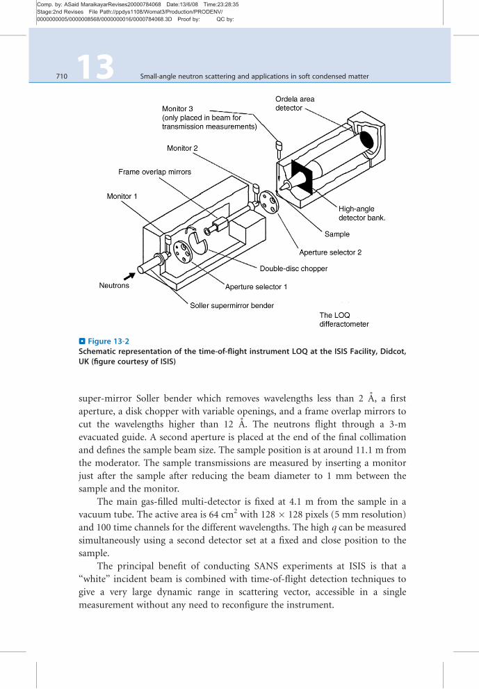
Comp. by: ASaid MaraikayarRevises20000784068 Date:13/6/08 Time:23:28:35Stage:2nd Revises File Path://ppdys1108/Womat3/Production/PRODENV/0000000005/0000008568/0000000016/0000784068.3D Proof by: QC by:
super-mirror Soller bender which removes wavelengths less than 2 A, a first
aperture, a disk chopper with variable openings, and a frame overlap mirrors to
cut the wavelengths higher than 12 A. The neutrons flight through a 3-m
evacuated guide. A second aperture is placed at the end of the final collimation
and defines the sample beam size. The sample position is at around 11.1 m from
the moderator. The sample transmissions are measured by inserting a monitor
just after the sample after reducing the beam diameter to 1 mm between the
sample and the monitor.
The main gas-filled multi-detector is fixed at 4.1 m from the sample in a
vacuum tube. The active area is 64 cm2 with 128 � 128 pixels (5 mm resolution)
and 100 time channels for the different wavelengths. The high q can be measured
simultaneously using a second detector set at a fixed and close position to the
sample.
The principal benefit of conducting SANS experiments at ISIS is that a
‘‘white’’ incident beam is combined with time-of-flight detection techniques to
give a very large dynamic range in scattering vector, accessible in a single
measurement without any need to reconfigure the instrument.
. Figure 13‐2Schematic representation of the time-of-flight instrument LOQ at the ISIS Facility, Didcot,UK (figure courtesy of ISIS)
710 13 Small-angle neutron scattering and applications in soft condensed matter

Comp. by: ASaid MaraikayarRevises20000784068 Date:13/6/08 Time:23:28:36Stage:2nd Revises File Path://ppdys1108/Womat3/Production/PRODENV/0000000005/0000008568/0000000016/0000784068.3D Proof by: QC by:
On LOQ at ISIS a pulse shaping 25 Hz disc shopper selects wavelength of
2.2–10 A, which are used simultaneously by time-of-flight.
For fixed geometry instruments working in time-of-flight mode, different
wavelength neutrons scattered at a same angle have different q values and arrive
on the detector at different times. The broader the incoming wavelength range,
the wider the q-range of the instrument. The data are saved in a 3D array with two
dimensions for the pixels of the detector and the third for the time axis.
The range of scattering vectors for time-of-flight instrument is similar to the
range of steady-state instruments. The main advantage of time-of-flight instru-
ment is that the full q-range is covered by only one instrument setting.
2.3 Detectors for SANS Instruments
Up to now, the most used detectors in SANS are gas proportional counters.
Until the end of 2003, D22 was handled with the largest area multidetector filled
with 3He as detection medium and CF4 as stopping gas. Technical data on
neutron detection are detailed in [9]. The neutron absorption by a target isotope
molecule (3He) induces a fission reaction and emission of two charged particles,
one triton and one proton, in opposite direction with a total kinetic energy of
760 keV which induces the primary ionization in gas. The stopping gas has two
roles. First it reduces the path length of the electrons for a good position
resolution and minimizes the wall effects. Secondly, in an environment of high
photon background, it has a low sensitivity to gamma and X-rays. The electrons
are accelerated to get more ionization and to amplify the signal. Near the anode
wire, where the electric field is very high, the ions produced by the electron
avalanche move away from the anode and induce a current in the cathode which
is measured.
On D22, the previous detector was composed by a network of 128 � 128
wires with a pixel size of 0.75 � 0.75 mm2. The advantages of gas-filled detectors
are their high efficiency for thermal neutrons, around 80% at a wavelength of 6 A
and a low sensitivity to g radiation.
The maximal count rate is limited by the time to collect the charges and the
electrons. The last developments on this field have permitted to decrease the dead
time down to t = 1 ns which represents a lost of 10% at 100 kHz count rate
(neutron/s). Dead time correction is possible and strongly improves the data
quality and curve overlapping. The two possible models are called paralyzable and
nonparalyzable. The ‘‘real’’ count rate Creal is calculated from the measured count
rate Cmes through the following relations.
Small-angle neutron scattering and applications in soft condensed matter 13 711

Comp. by: ASaid MaraikayarRevises20000784068 Date:13/6/08 Time:23:28:36Stage:2nd Revises File Path://ppdys1108/Womat3/Production/PRODENV/0000000005/0000008568/0000000016/0000784068.3D Proof by: QC by:
Nonparalyzable model:
Creal ¼ Cmes
1� tCmes
ð2Þ
Paralyzable model:
Creal ¼ Cmes exp �tCmesð Þ ð3ÞThe nonparalyzable model was used on D22 with the multiwire detector and is
still in use for data correction on D11 (ILL). More details can be found in [10].
Example of determination of detector dead time is presented in > Figure 13‐3.
The measurement done on the multiwires gas-filled detector from D22, consists
in measuring the attenuated direct beam through circular diaphragms and
increasing progressively the surface of the beam at the sample position. The
three attenuation factors are 147, 903, and 2,874. By considering a homogenous
beam, the flux is proportional to the beam surface. The full lines are the data
fitting with the nonparalyzable model, and the dotted lines are linear functions.
The dead time t is found at 0.91 ms, which corresponds to a lost 10% for a
measured count rate of 100 kHz (2).
Since March 2004, a new detector is operating on D22. The new detector
developed at the ILL by the detector group is a real-time neutron detector for
small-angle scattering applications, which is capable of counting 2 MHz of
neutrons on the whole detector with dead time losses of not more than 10%,
rather than the 100 kHz for the previous detector. This detector is composed of
. Figure 13‐3Dead time measurement on the gas-filled multiwire detector from D22. Flux measurementwith factor of attenuation of: (◊) F = 147, (□) F = 902, (D) F = 2874. The dotted lines are linearfunctions and full lines the fitting with the nonparalyzable equation (2)
712 13 Small-angle neutron scattering and applications in soft condensed matter

Comp. by: ASaid MaraikayarRevises20000784068 Date:13/6/08 Time:23:28:38Stage:2nd Revises File Path://ppdys1108/Womat3/Production/PRODENV/0000000005/0000008568/0000000016/0000784068.3D Proof by: QC by:
an array of 128 vertical tubes of 8 mm external diameter and 102 mm length
aligned side by side in a plan and brazed on both ends to a common pressure
vessel. The sensitive area is 1 m2, with a pixel size of 0.8� 0.8 mm2. The tubes are
filled with 3He and CF4 at 15 bars. The thin resistive anode wire is tightened in the
middle of the tube and relied on both sides of the amplifiers. The conversion of
neutrons to electrons follows the processes described previously. The impact
position along the tubes is now measured by charge division on the anode wire.
Finally, each tube is an independent counter able to reach 80 kHz at 10% dead
time correction. For very high count rates or localized spots due to pragg peaks
for example, a dead-time correction per tube can be performed. More details are
described in [11, 12].
For description of other neutron detectors, please refer to [9, 10, 13].
2.4 Sample Environments
The sample environment is easily versatile to match the various needs of the
users. Most of the SANS instruments possess a remotely controlled thermostatted
sample changer. Cryostats, cryofurnaces, furnaces, electromagnets are also avail-
able. A vacuum chamber can be used for very low scattering samples to reduce the
scattering from air.
The development of SANS experiments is strongly related to the develop-
ment of new sample environments, to investigate properties of sample under
nonsteady conditions. Shear apparatus, pressure cell, or stopped-flow apparatus
are more and more used routinely. Special equipments may also be developed and
designed by the scientist visitors (flash light [14], extruder [15], polarizer [16])
and adapted to the sample position.
3 Course of a SANS Experiment
3.1 Definition of the q-Vector
The schematic representation of a small-angle scattering experiment is presented
in > Figure 13‐4. In an ideal case, the neutron beam can be viewed as an assembly
of particles flying in parallel directions at a same speed. It can be described by a
planar monochromatic wave which the propagation equation can be written as:
f x; tð Þ ¼ f0e�i kt�oTð Þ ð4Þ
o ¼ 2p=T is the pulsation and ki is the incident wave vector; the magnitude is
k ¼ 2p=l. An atom scattered in the beam gives raise to a spherical wave. In SANS,
only the coherent elastic interaction between the neutron beam and the sample is
Small-angle neutron scattering and applications in soft condensed matter 13 713
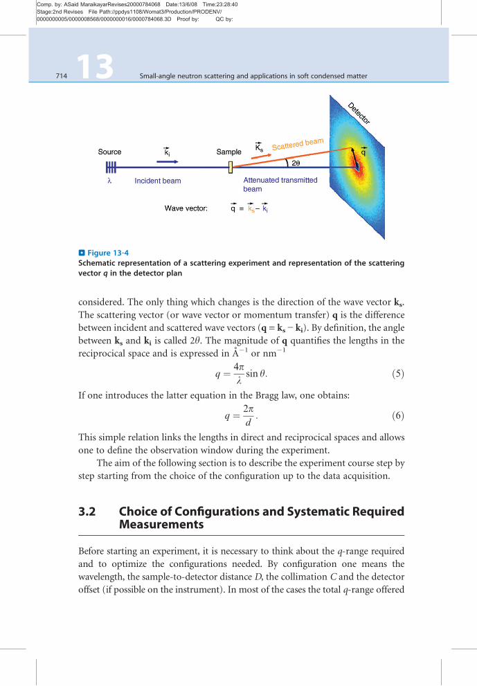
Comp. by: ASaid MaraikayarRevises20000784068 Date:13/6/08 Time:23:28:40Stage:2nd Revises File Path://ppdys1108/Womat3/Production/PRODENV/0000000005/0000008568/0000000016/0000784068.3D Proof by: QC by:
considered. The only thing which changes is the direction of the wave vector ks.
The scattering vector (or wave vector or momentum transfer) q is the difference
between incident and scattered wave vectors (q = ks − ki). By definition, the angle
between ks and ki is called 2y. The magnitude of q quantifies the lengths in the
reciprocical space and is expressed in A�1 or nm�1
q ¼ 4plsin y: ð5Þ
If one introduces the latter equation in the Bragg law, one obtains:
q ¼ 2pd: ð6Þ
This simple relation links the lengths in direct and reciprocical spaces and allows
one to define the observation window during the experiment.
The aim of the following section is to describe the experiment course step by
step starting from the choice of the configuration up to the data acquisition.
3.2 Choice of Configurations and Systematic RequiredMeasurements
Before starting an experiment, it is necessary to think about the q-range required
and to optimize the configurations needed. By configuration one means the
wavelength, the sample-to-detector distance D, the collimation C and the detector
offset (if possible on the instrument). In most of the cases the total q-range offered
. Figure 13‐4Schematic representation of a scattering experiment and representation of the scatteringvector q in the detector plan
714 13 Small-angle neutron scattering and applications in soft condensed matter
Comp. by: ASaid MaraikayarRevises20000784068 Date:13/6/08 Time:23:28:49Stage:2nd Revises File Path://ppdys1108/Womat3/Production/PRODENV/0000000005/0000008568/0000000016/0000784068.3D Proof by: QC by:
by the instrument is not necessary, and the limited beam time allocated per
experiment does not allow the users to investigate all the instrument possibilities.
If the largest size L of scatterers is roughly known (from any other tech-
nique), an evaluation of the minimum q is obtained by π/L. With a steady-state
instrument, it is recommended if possible to keep the wavelength constant and to
vary the sample-to-detector distance to cover the needed q-range. This choice
avoids repeating the transmission measurements and the calibrations that are
wavelength-dependent. It also facilitates the data treatment.
3.2.1 Collimation
The choice of the collimation distance is a compromise between the size of the
direct beam (and thus the resolution, see > Section 6 ) and the flux. Usually,
a collimation distance matching the sample-to-detector distance is used.
Nevertheless, for strong scatterer like water and/or short sample-to-detector
distance, larger collimation distances can be used to reduce the flux and the
scattering and to avoid detector saturation and damage.
A frequently chosen set of configurations onD22 is: l = 6 A,D = 17.5, 5, and 1.4
with an offset of the detector of 400mm to cover a q-range from 2 10�3 to 0.65 A�1.
The beginning of an experiment for each configuration requires, the alignment
of the beam-stop and measurement of beam center, electronic background, scatter-
ing of the sample empty cell and of a standard sample for absolute calibration.
3.2.2 Beam Center Determination
An attenuator is set in the direct beam and the beam-stop is removed. The
attenuated direct beam is measured through an empty position during several
tens of seconds. The beam center of gravity is calculated with standard routines
and further used for radial averaging. The integrated number of neutrons in the
direct beam allows one to calculate the flux if the attenuation factor is known.
3.2.3 Beam-Stop Alignment
The position of the direct beam on the detector varies with the sample-to-
detector distance, the collimation, and in an important way with the wavelength
since neutrons fall under gravity. Thus, the beam-stop position varies and the
Small-angle neutron scattering and applications in soft condensed matter 13 715
Comp. by: ASaid MaraikayarRevises20000784068 Date:13/6/08 Time:23:28:52Stage:2nd Revises File Path://ppdys1108/Womat3/Production/PRODENV/0000000005/0000008568/0000000016/0000784068.3D Proof by: QC by:
alignment has to be checked for each configuration, especially for large wave-
lengths and large sample-to-detector distances. A strong forward scatterer (teflon,
graphite, etc.) allows one to clearly see the shadow of the beam-stop, which is
correctly aligned when the same number of neutrons is counted on the beam-stop
edges (or on the first significant channel).
3.2.4 Electronic Background
The background is measured by stopping the incoming beam with a piece B4C or
Cadmium, which are both strong neutron absorbers (but Cd creates gammas). In
consequence what is measured on the detector comes from electronic noise,
cosmic, and instrument environment. These backgrounds are generally low.
Measurements are really important for weak scattering samples.
3.2.5 Standard for Calibration
The use of a standard has two functions: correction of the variation in cell
efficiency and normalization in absolute unit. Another possibility to get the
absolute scaling is to use standards with known cross section [17, 18]. For
SANS, samples with predominant incoherent scattering such as water (H2O) or
vanadium are currently used for the absolute scaling. With an ideal detector,
water shows a flat scattering independent from the scattering angle.
The water scattering is not measured at large sample-to-detector distances and
long collimation because the low flux would require several hours of acquisition to
get a good signal to noise ratio. The normalization and correction of cell efficiency
are done with a water run measured in another configuration but with the same
wavelength. The correction of flux and solid angle is explained in the next section.
It is recommended to perform the instrument calibrations and standard
measurements at the beginning of the experiment. Indeed, in case of instrument
failure, it will be nevertheless possible to treat the data recorded.
3.2.6 Transmission
The sample transmission is the ratio between the flux through the sample and the
incident flux at q = 0. The attenuated flux by the sample is measured in the same
way and conditions as the direct beam. A transmission measurement lasts less
than 5 min.
716 13 Small-angle neutron scattering and applications in soft condensed matter

Comp. by: ASaid MaraikayarRevises20000784068 Date:13/6/08 Time:23:28:52Stage:2nd Revises File Path://ppdys1108/Womat3/Production/PRODENV/0000000005/0000008568/0000000016/0000784068.3D Proof by: QC by:
3.2.7 Counting Time
For many samples, the scattering at large angles is strong but mainly due to
incoherent scattering coming from the sample and the solvent, especially for
hydrogenated solvent. Depending on the instrument and on the detector it is
known that a certain total number of neutrons NT on the whole detector area
will give after the radial averaging (in case of isotropic scattering) a good
statistics, i.e., small error bars and smooth shape of the curve. For example, on
D22, NT = 4,000,000 counts give good statistics. Short acquisitions of 10 s or less
allow one to estimate the sample count rate c/s. NT divided by c/s gives an
estimation of the acquisition time. The development of new ‘‘intelligent pro-
gram’’ able to stop an acquisition when a certain number of neutrons is reached
on the whole detector or in a defined area will be discussed in the last section
‘‘future and development.’’
The relevant count rate is the difference of count rates between the sample
and the solvent (mainly coming from incoherent diffusion). A too short mea-
surement especially at high q where the coherent intensity decreases give large
error bars on the absolute intensity and even negative values after subtraction of
background and incoherent scattering. It is recommended to measure the solvent
at large angles to have an experimental determination of the level of incoherent
scattering.
The number NT is of course just an indication that must be modulated in
function of the kind of information needed and also in function of the allocated
beam time. It can be reduced if statistics is not really needed (for example,
measurement of a slope) or increased in contrary if statistics is required (deter-
mination of a minimum, shape of Bragg peaks, etc.).
3.2.8 Command Files
Once the previous steps have been done, the configuration settings and the
acquisitions can be programmed in command files.
3.3 Conclusion
The choice of the configurations may be a determining factor for further analysis
and data fitting. It is a compromise between flux, resolution, beam time allocated,
and number of samples.
Small-angle neutron scattering and applications in soft condensed matter 13 717

Comp. by: ASaid MaraikayarRevises20000784068 Date:13/6/08 Time:23:28:53Stage:2nd Revises File Path://ppdys1108/Womat3/Production/PRODENV/0000000005/0000008568/0000000016/0000784068.3D Proof by: QC by:
4 From Raw Data to Absolute Scaling
The instruments from different Institutes have developed data treatment programs,
which can be adapted to other instruments after minor modifications for the
reading of data and parameters. The principle remains similar. For the ILL SANS
instruments see [19] for the standard programs in use. The different steps consist in:
� Calculating the beam center for the different configurations used.
� Creating mask files to hide cells behind the beam stop as well as potential ‘‘bad cells’’
� Calculating transmissions.
� Performing radial averaging giving the intensity as a function of q in case of isotropic
scattering. Depending on the programs, what is called ‘‘intensity’’ at this step can be
a number of neutrons, or a count rate per second or per monitor unit.
� The last step to obtain the absolute intensity is more delicate and its description is
the aim of the following section.
(1) Note: The two last points can be performed in the reverse order. Absolute
scaling can be performed on the 2D image, before radial or section averaging for
anisotropic data.
When a coherent beamwith a fluxFo illuminates a sample of volume Vand a
thickness e, during a time t, a given fraction of the incident flux DN is elastically
scattered in the direction q within a solid angle DΩ:
DN ¼ F0tTrdsdO
ðqÞDO; ð7Þwhere Tr is the transmission of the sample.
dsdO ðqÞ is the differential scattering cross section characteristic of elastic
interaction between sample and neutrons. Then the intensity I scattered per
unit volume is
I cm�1� � ¼ 1
V
dsdO
ðqÞ ¼ DN qð ÞF0Tr DOð Þ:t:e
dSdO
� �Total
¼ N qð ÞFo:DO qð Þ:Tr:t:e ¼
1
FoDO qð Þ:Tr qð Þ:t:e qð Þ I qð Þ: ð8Þ
In soft condensed matter, the samples are generally filled in a quartz cell that
contributes slightly to the general scattering. The scattering from the empty cell
(EC) is subtracted from the total scattering as follows:
dSdO
� �sample
¼ 1
esample
Nsample qð ÞFo:DO qð Þ:Trsample:tsample
� NEC qð ÞFo:DO qð Þ:TrEC:tEC
" #sample
¼ 1
esampleFo
Nsample qð ÞDO qð Þ:Trsample:tsample
� NEC qð ÞDO qð Þ:TrEC:tEC
" # ð9Þ
718 13 Small-angle neutron scattering and applications in soft condensed matter

Comp. by: ASaid MaraikayarRevises20000784068 Date:13/6/08 Time:23:28:57Stage:2nd Revises File Path://ppdys1108/Womat3/Production/PRODENV/0000000005/0000008568/0000000016/0000784068.3D Proof by: QC by:
(2) In the case of a solid sample, which does not necessitate a cell, the scattering
from air has to be removed.
The transmissions are calculated with respect to the empty beam.
We now turn to the description, calculation, or measurement of the different
terms of the previous equation.
4.1 Determination of the Incident Flux F0
In (7), the incident flux F0 is the number of neutrons per second at the sample
position for a given aperture. The flux can be measured directly with a calibrated
monitor installed at the sample position. The other possibility is to measure the
direct beam on the detector through a calibrated attenuator. This approach calls
SEB, the sum of neutrons integrated in the surface of the direct beam, tEB, the
acquisition time, and F, the factor of attenuation. Then, taking into account the
detector dead time t
F0 n=sð Þ ¼ FSEB=tEB
1� tSEB=tEB: ð10Þ
Thanks to the development of new fast detectors like the one on D22 at the ILL,
the dead time correction is not necessary in most of the cases. For classical gas
detectors, the dead time is of the order of few tens of microseconds and corre-
sponds to a lost of 10% of neutrons at count rates of 100 kHz.
4.2 Normalization with a Standard Sample
Samples with predominant incoherent scattering such as light water (H2O) or
vanadium are used for the absolute scaling and to correct the variations in
efficiency of the cells.
dSdO
� �sample
¼ Isample
Istandard
dSdO
� �standard
ð11Þ
A water sample of thickness e = 0.1 cm is frequently used as standard because
water is easy to find, the liquid is homogenous at the scales of SANS, and the
scattering is mainly incoherent. However, due to inelastic and multiple scattering
effects, the water scattering is not totally isotropic, but stronger in the forward
direction. The assumption that the neutrons that are not transmitted are scattered
uniformly in 4p steradians is wrong. A wavelength-dependent correction factor
g(l) has to be introduced to write the real scattering cross section
Small-angle neutron scattering and applications in soft condensed matter 13 719
Comp. by: ASaid MaraikayarRevises20000784068 Date:13/6/08 Time:23:29:00Stage:2nd Revises File Path://ppdys1108/Womat3/Production/PRODENV/0000000005/0000008568/0000000016/0000784068.3D Proof by: QC by:
dSdO
� �real
H20
¼ g lð Þ 1� Tr
4p:e:Tr: ð12Þ
In SANS there is no universal calibration curves. The water scattering measured on
two instruments may vary significantly. Because of multiple scattering and inelastic
effects, scattering depends on the wavelength distribution, on the geometry and
configuration, and on the detector. Between D11 and D22, when both instruments
are working with a gas-filled detector, the difference of g(l) values was of the orderof few percents. As long as possible, it is thus extremely important to carry out the
calibrations in the same setting conditions as the samples.
dS=dOð ÞrealH2Ocan be calculated using (9). It is also possible to recalculate
dS=dOð ÞrealH2Oby measuring standards (polymer) from samples with a known
cross section [17, 18].
dS=dOð ÞrealH2Oas a function of l may be empirically extrapolated with a
polynomial function:
dS=dOð ÞrealH2O¼ Aþ B:lþ C:l2 þD:l3
The water cross-section increases with the wavelength and varies slightly with
temperature. The values are close to 1 cm�1.
Sample normalization using water as standard is obtained according the
following equation:
dSdO
� �sample
¼ 1
Fsc
dSdO
� �real
H2O
Isample � IB4C
Trsample
� Isample�EC � IB4C
Trsample�EC
� �1
esample
IH2O�IB4C
TrH2O� IH2O�EC�IB4C
TrH2O�EC
h i1
eH2O
ð13Þ
The subscript EC refers to the empty cell. Tr is the transmission with respect to
the empty beam, I is the number of neutrons per second. Fsc is a scaling
coefficient equal to 1 when the water and the sample are measured in the same
instrument configuration. For large sample-to-detector distance (D > 10 m) and
thus large collimation, the flux and water count rates are too low to get a good
statistics in a reasonable time. A water run measured in a configuration with
higher flux (at shorter sample to detector distance) but the same l is used to
correct the variations of detector efficiency. Then, the scaling factor Fsc corrects
the flux that varies with the collimation and the solid angle according to
F ¼ F0DOð Þsample
F0DOð ÞH2O
¼ CollH2ODH2O
CollsampleDsample
� �2
¼ Fsample
FH2O
DH2O
Dsample
� �2
; ð14Þ
where Dsample and Dwater are the sample-to-detector distances; Collsample and
Collwater are the collimations, and Fsample and Fwater are the fluxes at the sample
position in the two configurations.
720 13 Small-angle neutron scattering and applications in soft condensed matter

Comp. by: ASaid MaraikayarRevises20000784068 Date:13/6/08 Time:23:29:06Stage:2nd Revises File Path://ppdys1108/Womat3/Production/PRODENV/0000000005/0000008568/0000000016/0000784068.3D Proof by: QC by:
The other possibility to calculate dS=dOð ÞrealH2Ois to apply (2), the delicate
point being the accurate measurement of Fo.
4.3 Solid Angle DV(Q)
> Figure 13‐5 presents the geometry of a scattering experiment when the detector
is close to the sample position. The scales are not respected in order to put in
evidence the different angles and distances. O is the origin of the scattered beams
(sample position) and O0 the image of the direct beam on the detector. 2y is the
scattering angle O 0OO 00, also equal to the angle defined by ADA0. The sample-to-
detector distance is represented by the segment D 2yð Þ ¼ OO 0 0 and p ¼ A0B 0 isthe pixel size. D 0ð Þ ¼ OO0
The sample-to-detector distance and the solid angle are function of
2y according to
DO 2yð Þ ¼ AB2.
D 2yð Þ½ �2
;
D 2yð Þ ¼ D 2y ¼ 0ð Þ=cos 2yð Þ and AB ¼ p2 cos 2yð Þ:Finally
DO 2yð Þ ¼ p2 cos3 2yð ÞD 2y ¼ 0ð Þ : ð15Þ
Equation (15) shows that the solid angle value decreases with q. An example is
shown in > Figure 13‐6, where water was measured with the following configura-
tion: D = 1.4 m, C = 17.6 m, and l = 6 A. The data are normalized in absolute
. Figure 13‐5Geometric representation of scattered beams: determination of detector distance and solidangle as a function of 2u, the scattering angle
Small-angle neutron scattering and applications in soft condensed matter 13 721

Comp. by: ASaid MaraikayarRevises20000784068 Date:13/6/08 Time:23:29:12Stage:2nd Revises File Path://ppdys1108/Womat3/Production/PRODENV/0000000005/0000008568/0000000016/0000784068.3D Proof by: QC by:
scale according to (8). The hollow diamonds are obtained taking the solid angle as
a constant. One observes a strong decrease of the intensity as q increases. The full
symbols are calculated using (15) which allows one to get the flat scattering
expected for incoherent scatterers. The slight decrease still remaining at high q
can be due to inelastic effects in light water.
4.4 Transmission
4.4.1 Definition
The transmission is the ratio of the intensities at q = 0 between the beam through
the sample and the white beam. It depends on the sum of coherent, incoherent,
and absorption cross-sections and also from the scattering angle.
Tr 2y; lð Þ ¼ I 2yð ÞI0
¼ exp �m lð Þe 2yð Þð Þ;
TrðlÞ ¼ Ið0ÞI0
¼ exp �Ns lð Þe 2yð Þð Þ ¼ exp �m lð Þe 2yð Þð Þ ¼ exp �e 2yð Þ=L lð Þð Þ;ð16Þ
Where m lð Þ, the mass adsorption coefficient is wavelength-dependant andL lð Þ isthe mean free path of the radiation in the sample. s lð Þ can be calculated from the
transmission measured at y = 0 and is the sum of three terms:
s lð Þ ¼Xi
scoh;i þ sincoh;i þ sabs;i lð Þ ð17Þ
. Figure 13‐6Water scattering measured on D22 at short sample-to-detector distance, D = 1.4 m,C = 17.6 m, l = 6 A. The raw data are normalized in absolute scale according to (1.8).(◊) DV kept constant at p2/D(0)2; (♦) DV calculated with (15) to correct from geometricdistortion
722 13 Small-angle neutron scattering and applications in soft condensed matter
Comp. by: ASaid MaraikayarRevises20000784068 Date:13/6/08 Time:23:29:12Stage:2nd Revises File Path://ppdys1108/Womat3/Production/PRODENV/0000000005/0000008568/0000000016/0000784068.3D Proof by: QC by:
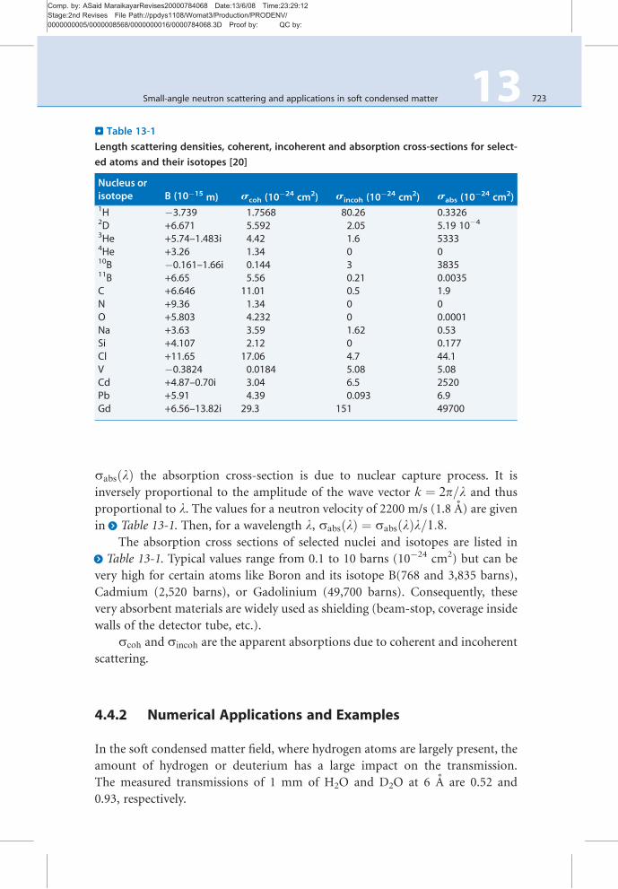
sabs lð Þ the absorption cross-section is due to nuclear capture process. It is
inversely proportional to the amplitude of the wave vector k ¼ 2p=l and thus
proportional to l. The values for a neutron velocity of 2200 m/s (1.8 A) are given
in >Table 13-1. Then, for a wavelength l, sabs lð Þ ¼ sabs lð Þl=1:8.The absorption cross sections of selected nuclei and isotopes are listed in
>Table 13-1. Typical values range from 0.1 to 10 barns (10�24 cm2) but can be
very high for certain atoms like Boron and its isotope B(768 and 3,835 barns),
Cadmium (2,520 barns), or Gadolinium (49,700 barns). Consequently, these
very absorbent materials are widely used as shielding (beam-stop, coverage inside
walls of the detector tube, etc.).
scoh and sincoh are the apparent absorptions due to coherent and incoherent
scattering.
4.4.2 Numerical Applications and Examples
In the soft condensed matter field, where hydrogen atoms are largely present, the
amount of hydrogen or deuterium has a large impact on the transmission.
The measured transmissions of 1 mm of H2O and D2O at 6 A are 0.52 and
0.93, respectively.
. Table 13‐1Length scattering densities, coherent, incoherent and absorption cross-sections for select-
ed atoms and their isotopes [20]
Nucleus orisotope B (10�15 m) scoh (10
�24 cm2) sincoh (10�24 cm2) sabs (10
�24 cm2)1H �3.739 1.7568 80.26 0.33262D +6.671 5.592 2.05 5.19 10�4
3He +5.74–1.483i 4.42 1.6 53334He +3.26 1.34 0 010B �0.161–1.66i 0.144 3 383511B +6.65 5.56 0.21 0.0035C +6.646 11.01 0.5 1.9N +9.36 1.34 0 0O +5.803 4.232 0 0.0001Na +3.63 3.59 1.62 0.53Si +4.107 2.12 0 0.177Cl +11.65 17.06 4.7 44.1V �0.3824 0.0184 5.08 5.08Cd +4.87–0.70i 3.04 6.5 2520Pb +5.91 4.39 0.093 6.9Gd +6.56–13.82i 29.3 151 49700
Small-angle neutron scattering and applications in soft condensed matter 13 723
Comp. by: ASaid MaraikayarRevises20000784068 Date:13/6/08 Time:23:29:12Stage:2nd Revises File Path://ppdys1108/Womat3/Production/PRODENV/0000000005/0000008568/0000000016/0000784068.3D Proof by: QC by:
The absorption of air is of 1% per meter. For long instruments as SANS
spectrometers, it is then important to keep the neutron guides and the detector
tankunder vacuum. In some cases, 4He is used to fill the neutron guides. A guide of
1 m length filled with 4He at atmospheric pressure is considered. Helium density
is d = 0.2 g/cm3. The molecule number per cm3 is dN ¼ dNa=M, with Na the
Avogadro number andM the molar mass. For a length of 1 m, the transmission is
Tr¼ exp �dNsTLð Þ, with dN = 0.301 � 1020 mol/cm3, sT = 1.34 � 10�24 cm2,
and L = 100 cm, then Tr = 0.996. The absorption is nearly negligible, muchweaker
than air. Nowwith 3He in the same conditions, sT �sa ¼ 5333� 10�24l=1:8cm2
and Tr � 10�7.
4.4.3 Transmission at Large Angles
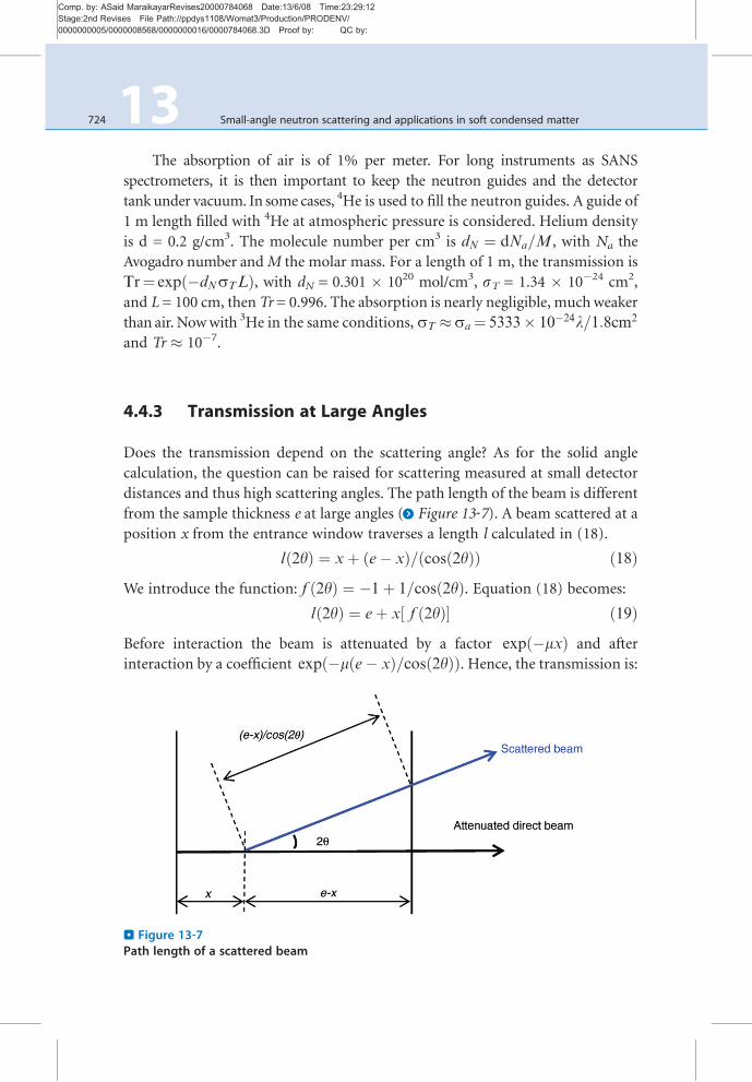
Does the transmission depend on the scattering angle? As for the solid angle
calculation, the question can be raised for scattering measured at small detector
distances and thus high scattering angles. The path length of the beam is different
from the sample thickness e at large angles (> Figure 13‐7). A beam scattered at a
position x from the entrance window traverses a length l calculated in (18).
l 2yð Þ ¼ xþ e� xð Þ= cos 2yð Þð Þ ð18ÞWe introduce the function: f 2yð Þ ¼ �1þ 1=cos 2yð Þ. Equation (18) becomes:
l 2yð Þ ¼ eþ x f 2yð Þ½ � ð19ÞBefore interaction the beam is attenuated by a factor exp �mxð Þ and after
interaction by a coefficient exp �m e� xð Þ=cos 2yð Þð Þ. Hence, the transmission is:
. Figure 13‐7Path length of a scattered beam
724 13 Small-angle neutron scattering and applications in soft condensed matter

Comp. by: ASaid MaraikayarRevises20000784068 Date:13/6/08 Time:23:29:17Stage:2nd Revises File Path://ppdys1108/Womat3/Production/PRODENV/0000000005/0000008568/0000000016/0000784068.3D Proof by: QC by:
Tr 2yð Þ ¼ 1e
Ðe0
exp �m eþ xf 2yð Þð Þ½ �dx ¼ 1eexp �með Þ Ðe
0
exp �mxf 2yð Þ½ �dxTr 2yð Þ ¼ mef 2yð Þ½ ��1
exp �með Þ 1� exp �mef 2yð Þ½ �f gð20Þ
The dependence of transmission as a function of 2y and q , is presented for light
and heavy water in > Figure 13‐8. At q = 0.8 A−1 the diminution of the transmis-
sion is of only 3% for D2O and can be neglected. The decrease is of 23% for
H2O and a connection must be taken into account during data reduction.
4.5 Multiple Scattering
Multiple scattering occurs when a scattered neutron is scattered again in the sample.
There is always a probability that such event occurs but it must not dominate the
total scattering.Multiple scattering smears the true intensity since the total intensity
is the sum of intensities due to single, twice, or more scattering vectors at unknown
angles. The data interpretation becomes nearly impossible or wrong, if the multiple
scattering is not detected. Suspicion of multiple scattering can be done in case of
low transmission (<0.5) and strong scattering intensity at low q (>104 cm�1).
There is no general method to correct data from multiple scattering but in case of
‘‘weak’’ multiple scattering, different methods are proposed [21]. A criterion to
. Figure 13‐8Transmission of light and heavy water as a function of the scattering angle and scatteringvector. For l = 6 A, m(H2O) = −6.539 cm−1 and m(D2O) = −0.726 cm−1 calculated fromexperimental transmission measurements on D22
Small-angle neutron scattering and applications in soft condensed matter 13 725

Comp. by: ASaid MaraikayarRevises20000784068 Date:13/6/08 Time:23:29:18Stage:2nd Revises File Path://ppdys1108/Womat3/Production/PRODENV/0000000005/0000008568/0000000016/0000784068.3D Proof by: QC by:
avoid multiple scattering has been given in [22] and says that ‘‘part of attenuation
of the direct beam due to coherent scattering should not be <9.’’ This result has
been established with studies on interpenetrating polymer networks.
4.5.1 Transmission at Large Angles
In case of low multiple scattering, the effect is not easily detected. Different
scattering distortions are observed. First evidence is that several curves measured
at different configurations do not overlap. In case of fractal dimension, at low q, the
multiple scattering induces a lowering of the intensity that could be confused with a
plateau. Artifacts due to multiple scattering are presented in > Figure 13-9. The
sample consists in a dispersion of carbon black particles in amatrixmade of styrene-
butadiene rubber [23]. The green squares (□) corresponds to a sample thickness
e=1.3mm,measured at l = 20 A (transmission Tr= 0.02). The data reach a plateau
at q = 0.01 A�1. The blue diamond (◊) have been obtained with a half-thickness
sample, e = 0.63 mm and l = 20 A (Tr = 0.08). The down-turn is less pronounced
but still present. The last curve (○) where the thickness is only 1 mmwas measured
at l = 5 A (Tr = 0.88). After comparison with X-ray data (not shown), it has been
proved that only the latter curve does not suffer from multiple diffusion.
With concentrated microemulsions, it has been observed on the contrary, an
increase in the low q scattering and of the width of the correlation peak, with a
. Figure 13‐9Evidence of multiple scattering on a sample made of carbon black particles dispersed in anelastomer matrix. (□) e = 1.3 mm, l = 20 A; (◊) e = 0.63 mm, l = 20 A: (○) e = 1 mm, l = 5 A
726 13 Small-angle neutron scattering and applications in soft condensed matter

Comp. by: ASaid MaraikayarRevises20000784068 Date:13/6/08 Time:23:29:19Stage:2nd Revises File Path://ppdys1108/Womat3/Production/PRODENV/0000000005/0000008568/0000000016/0000784068.3D Proof by: QC by:
multiple image of the main scattering peak and an increase of the incoherent
background [24].
4.5.2 How to Prevent Multiple Scattering?
� Use thinner sample, use diluted sample (if dilution does not induce phase transition)
� Use shorter wavelength to increase the mean free path Λ(l)� Decrease the contrastDr (for example, use deuterated compound in deuteratedmatrix)
4.6 Subtraction of Incoherent Background
The incoherent scattering, mainly coming from the hydrogen molecules, gives
raise to a flat background that is necessary to subtract before the data analysis.
The subtraction is a delicate point, since an under or upper estimation of the
incoherent background may vary a slope or the position of a minimum in q and
thus alter the data interpretation. Different methods are then employed.
� The incoherent background can be estimated with the measurement at the highest
possible scattering vector q (>0.4 A�1) because in most of the cases in soft
condensed matter the objects are big and the coherent scattering becomes negligible.
� In case of very dilute deuterated compound in hydrogenated solvent, the subtraction
of the scattering from the solvent will be sufficient.
� A reference sample with no structure and containing the same amount of H and D
molecules (for example, a mixture of H2O/D2O) can be measured. This requires to
know exactly the sample composition or to prepare a mixture having the same
transmission as the sample.
� If the scattering cross section as a q dependence, one can write:
dSdO / Aq�d þ B; where B represents the background. At high q, one can
suppose that the Porod regime is reached, then dS�dOq4 / Aþ Bq4. The slope
gives the value of the incoherent background. This simple empirical method gives
reasonable results.
� The incoherent background can be calculated in principle with the tabulated values of
binc. Nevertheless, the values are given for bound atoms, and are smaller than the real
ones. Moreover, the incoherent contribution coming from the spin is not taken into
account.
Small-angle neutron scattering and applications in soft condensed matter 13 727
Comp. by: ASaid MaraikayarRevises20000784068 Date:13/6/08 Time:23:29:19Stage:2nd Revises File Path://ppdys1108/Womat3/Production/PRODENV/0000000005/0000008568/0000000016/0000784068.3D Proof by: QC by:
4.7 Conclusion
The data reduction is a crucial step before data analysis. Particular care must
be taken in the high-angle scattering due to corrections for the solid angle,
transmission and the incoherent scattering, as described in a recent article [24].
The importance of the absolute calibration is obvious. SANS curves obtained
on different spectrometers or in different q-ranges can be joined together and
compared. Absolute intensity allows one to calculate molecular mass, volume
fraction, specific area of scattering elements, etc. It also can prove the presence of
multiple scattering, repulsive or attractive forces, unexpected aggregation, or
sample degradation. In addition length scattering densities can be extracted and
hydration numbers deduced.
The experimental intensity in absolute scale cm�1 as a function of the
scattering vector q is now established. The standard models to be compared
with the experiment will be described in the following section.
5 Modeling of the Scattered Intensity
A detailed theory of small-angle scattering can be found in [2, 25]. In this section,
only the basis equations will be introduced and stress will be put on analytic
expressions widely used and illustrated by recent experiments.
The interaction with the neutron beam depends on the kind of atom i. The
scattering probability is proportional to a surface sis, characteristic from the
interaction between the radiation and the atom. This surface is the scattering
cross section and corresponds to the atom surface seen by the radiation. The cross
section is equal to sis ¼ 4p bij j2
D E. bi is the scattering length which characterizes
the range of interaction. The scattering length density (SLD) is then equal to
r rð Þ ¼Pi
ri rð Þbi; where ri rð Þ is the local density of atom i. Basic relationships
between the neutron scattering lengths and cross sections, dependencies on the
spin and values are tabulated in [20]. Some of them are given in >Table 13-1.
The differential cross-section is related to the amplitude of the scattered
wave by
dsdO
¼ bj j2:
5.1 Rules of Thumb in Small-Angle Scattering
We consider a statically isotropic system where the particle positions are not
correlated at long range. In the Born approximation, the interaction with a
728 13 Small-angle neutron scattering and applications in soft condensed matter

Comp. by: ASaid MaraikayarRevises20000784068 Date:13/6/08 Time:23:29:20Stage:2nd Revises File Path://ppdys1108/Womat3/Production/PRODENV/0000000005/0000008568/0000000016/0000784068.3D Proof by: QC by:
scatterer does not depend on the scattering by the other scatterers. In this case,
the amplitude scattered by the different particles can be added. For a particle
of length scattering density r(r), the amplitude is given by:
A qð Þ ¼ðV
r rð Þe�iqrdr ð21Þ
r rð Þ describes the distribution of length densities in the particle and is directly
related to the chemical composition. It is convenient to split r rð Þ into two parts
and to put in evidence the fluctuations around an average value:
r rð Þ ¼ rh i þ dr rð Þ: ð22Þ
The contribution from the average term is null for q > 0, then
A qð Þ ¼ðV
dr rð Þe�iqrdr: ð23Þ
The detector measures the intensity which is the absolute square of the ampli-
tude. The scattered intensity per unit volume is:
I qð Þ ¼ A qð ÞA� qð ÞV
¼ 1
V
ððVV
dr rð Þdr r0ð Þe�iqðr�r0Þdrdr0: ð24Þ
In the simplest case where the system is made of two phases, one of length
scattering density rp and the second one of length scattering density rs, (24)becomes:
I qð Þ ¼ 1
Vrp � rS 2 ð
Vp
ðVp
e�iq r�r0ð Þdrdr0 ¼ 1
VDr2
ðVp
ðVp
e�iq r�r0ð Þdrdr0 ð25Þ
Dr is the difference of length scattering densities between particle and matrix. An
assembly of Np identical particles is next considered. Equation (25) can be
rewritten as:
I qð Þ ¼ V 2p
VNpDr2 F qð Þ½ �2; with F qð Þ ¼ 1
Vp
ðVp
e�iqrdr; ð26Þ
Finally, with the usual notations, one gets:
I qð Þ ¼ FVpDr2P qð Þ ð27Þ
Small-angle neutron scattering and applications in soft condensed matter 13 729

Comp. by: ASaid MaraikayarRevises20000784068 Date:13/6/08 Time:23:29:20Stage:2nd Revises File Path://ppdys1108/Womat3/Production/PRODENV/0000000005/0000008568/0000000016/0000784068.3D Proof by: QC by:
P(q) is called the particle form factor and describes the geometry of the scattering
object. P(q) tends to 1 for q = 0.
We consider now an assembly of Np identical particles correlated in space.
The measured intensity is equal to the statistical average over all the particle
positions and orientations in a volume V:
I qð Þ ¼ A qð ÞA� qð ÞV
¼ 1
V
ðV
r rð Þe�iqrdr
ðV
r r0ð Þe�iqr0dr0* +
ð28Þ
Let us write r as r = ri + u,
I qð Þ ¼ 1
V
Xi
e�iqri
ðVp
r uð Þe�iquduXj
e�iqrj
ðVp
r vð Þe�iqvdv
* +ð29Þ
For spherical particles with identical interactions, the average of the product is
equal to the product of the averages, then:
I qð Þ ¼ N
V
1
N
XNi¼1
XNj¼1
e�iq ri�rjð Þ" # ð
Vp
ðVp
r uð Þr vð Þe�iqðu�vÞdudv
264
375
* +: ð30Þ
One recognizes in the second term the particle form factor. The first term is the
structure factor S(q) describing the correlation between particle mass centers. If
one excludes the case ri = rj then the expression for the structure factor becomes:
S qð Þ ¼ 1þ 1
N
XNi¼1
Xj 6¼i
e�iq ri�rjð Þ* +
: ð31Þ
In a continuous medium, (31) can be written as:
S qð Þ ¼ 1þN � 1
V
ðV
g rð Þe�iqrdr; ð32Þ
where g(r) is the correlation function between particle mass centers. At q = 0,
according to (31) S(q) = N.
We define the following function Sm qð Þ as
Sm qð Þ ¼ S qð Þ �N � 1
Vd qð Þ: ð33Þ
With d the Dirac function. Then,
Sm qð Þ ¼ 1þN � 1
V
ðV
g rð Þ � 1½ �e�iqrdr: ð34Þ
730 13 Small-angle neutron scattering and applications in soft condensed matter
Comp. by: ASaid MaraikayarRevises20000784068 Date:13/6/08 Time:23:29:20Stage:2nd Revises File Path://ppdys1108/Womat3/Production/PRODENV/0000000005/0000008568/0000000016/0000784068.3D Proof by: QC by:
In the case of isotropic interactions, azimuthal (radial) averaging reduces (34) to:
Sm qð Þ ¼ 1þN � 1
V
ðV
4pr2 g rð Þ � 1½ � sin qrqr
dr: ð35Þ
To summarize, the intensity per unit volume V of Np homogeneous isotropic
scatterers of volume Vp and coherent length scattering density rp dispersed in a
medium of length scattering density r is the product of the form factor and the
structure factor weighted by a contrast factor Kc follows:
I qð Þ ¼ FVpDr2P qð ÞS qð Þ ¼ KcP qð ÞS qð Þ: ð36ÞIn the following, the three relevant parts of the above equation, r, P(q), and S(q)
will be detailed and numerical applications will be described to aid in the
understanding and interpretation of scattering curves.
5.2 SLD, Contrast Variation, and Isotopic Labeling
The SLD from a molecule with xi, atoms i and molecular volume vp is:
rp ¼Pi
xibi
vpð37Þ
bi is the coherent neutron scattering length of atom i. Only coherent scattered
neutrons carry information about structure. The molecular volume vp requires
knowledge of the bulk density of the molecule. It can be difficult to measure and
is a source of inaccuracy on the SLD value. r is usually expressed in cm�2 or A�2.
The calculation of the atomic bi is not trivial and values are experimentally
determined and tabulated [20]. The magnitude is determined by the quantum
mechanics of the neutron–nucleus interaction. It varies in an unsystematic way
with the atomic number, depending on the direction of the nuclear spin and
drastic variations can be found between two isotopes, the main example being the
difference of value and sign between hydrogen and deuterium atoms. A negative
value signifies a shift of p of the phase on scattering.
This last property is of great importance and opens the possibility of what is
called ‘‘contrast variation.’’ The principle is to substitute one atom by one of its iso-
topes to induce a strong variation in the scattering length, assuming that no drastic
perturbation of the properties (physical, chemical, etc.) of the sample occurs.
In soft condensed matter, the compounds of interest (colloids, emulsions,
surfactants, polymers, etc.) contain a large quantity of hydrogen molecules which
can be substituted in principle by deuterium atoms and bH = �0.374 10�12 cm�2
Small-angle neutron scattering and applications in soft condensed matter 13 731
Comp. by: ASaid MaraikayarRevises20000784068 Date:13/6/08 Time:23:29:20Stage:2nd Revises File Path://ppdys1108/Womat3/Production/PRODENV/0000000005/0000008568/0000000016/0000784068.3D Proof by: QC by:
and bD = 6.37 10�12 cm�2. This feature is at the origin of many SANS experi-
ments and important advancements have been done in the description of mole-
cular assemblies. One of the pioneering studies using the contrast variation
method has been carried out by Stuhrmann in 1974 at the ILL [3–5] to investigate
the structure of biological macromolecule like ferritin. In the first article the
author concludes that ‘‘the most promising domain of neutron small-angle
scattering seems to be the study of H-D exchange of reactions of macromolecules
in dilute solutions.’’ Thirty years later, this conclusion is still relevant.
Isotopic substitution can be used to create a contrast inside a particle by a
specific labeling of a part of the molecule. In the field of polymer science, the
technique is widely used. For example, the difference in length scattering density
between hydrogenated and deuterated polystyrene (rPSH = 1.42� 1010 cm�2 and
rPSD = 6.42 � 1010 cm�2) was used to follow the chain conformation during
extrusion of a polymer melt made of a few percent (ca. 5%) of hydrogenated
polystyrene mixed with deuterated polystyrene [15].
5.2.1 The Zero Average Contrast Method
For semidiluted polymer or polyelectrolyte solutions, both intra- and intercorre-
lations between the polymer chains contribute to the scattered intensity. The zero
average contrast (ZAC) method allows the elimination of the signal coming from
the structure factor (the intercorrelations) to see only the form factor from a
single chain. The method consists in the exchange of hydrogen by deuterium
atoms in the polymer chain and the modification of the length scattering density
of solvent by a mixture of hydrogenated and deuterated molecules.
We consider a polymer solution containing Nh and Nd, H- and D-polymer
chains, with Nh and Nd monomers, respectively. The volume fraction of deuter-
ated monomers is called F. The ZAC is obtained when the following condition is
fulfilled:
1� Fð ÞDrH þ FDrD ¼ 0; ð38Þwhere DrH and DrD are the differences of length scattering densities from the
H- and D- monomers and the solvent, respectively. Different examples of ZAC
applications are illustrated by the references given in [27]. The experiments have
demonstrated the vermicular form factors of fully charged PSSNa polymer
chains. Reference [28] presents a study of polystyrene in diethylphalate in good
solvant where the form factor of a single chain as a function of the shear rate is
investigated.
732 13 Small-angle neutron scattering and applications in soft condensed matter

Comp. by: ASaid MaraikayarRevises20000784068 Date:13/6/08 Time:23:29:20Stage:2nd Revises File Path://ppdys1108/Womat3/Production/PRODENV/0000000005/0000008568/0000000016/0000784068.3D Proof by: QC by:
5.2.2 Contrast Variation Technique
One of the main applications is found in multiple component systems to match a
compound or a part of aggregate with a specific isotopic mixture of solvent. This
technique called ‘‘contrast match’’ has been successfully used to elucidate the
structure of particles composed of different layers, as for example, in microemul-
sions; to investigate surfactant layers adsorbed around mineral particles [29]; and
for characterization of complex systems [30].
We recall that the scattered intensity for a dilute system without interaction is:
I qð Þ ¼ FVp Drð Þ2P qð Þ: ð39ÞAt q = 0, P(q) tends to 1 and
I 0ð Þ ¼ FVp Drð Þ2¼ FVp rp � rs 2
: ð40Þ
rp is the average scattering density of the solute and rs that of solvent or matrix.
The knowledge of the molecular volume is sometimes a delicate point,
and the calculation of rp is extremely sensitive to Vp, the volume in bulk and
thus to the density d since Vp ¼ M=d , M being the molar mass. In such cases
d can be accurately determined by measuring the length scattering density of the
molecule.
The average length scattering density of a H/D mixture is:
rs ¼ xrDs þ 1� xð ÞrHs ð41Þwith x the volume fraction of deuterated solvent.
ffiffiffiffiffiffiffiffiffiffiffiffiffiffiffiffiffiffiffiI q ! 0ð Þp / � Drð Þ is linear
as a function of x if the particles are monodisperse. At contrast match I(0) = 0 one
can deduce x and rp. For polydisperse particles in solution, the intensity is never
zero, and only a minimum is obtained.
Experimentally, a contrast variation experiment consists in measuring the
scattered intensity at the lowest possible q. The samples prepared at the same
concentration in different mixtures of D/H solvent, from fully deuterated to fully
hydrogenated solvent. The following example presents an experimental determi-
nation of the SLD of laponite particles from a contrast variation experiment
(> Figure 13‐10). Laponite is a synthetic clay which the particles have been
characterized by other techniques as well (cryofracture and TEM [32]; AFM
[31]). The particles can be described as monodisperse disks of 1 nm thickness
and 30 nm diameter. The general composition is Si8Mg5.45Li0.4H4O24Na0.7, den-
sity 2.65, and the volume of the unit cell is 4.7847 10�22 cm3. One gets
rlaponite = 3.94.1010 cm�2.
Small-angle neutron scattering and applications in soft condensed matter 13 733

Comp. by: ASaid MaraikayarRevises20000784068 Date:13/6/08 Time:23:29:20Stage:2nd Revises File Path://ppdys1108/Womat3/Production/PRODENV/0000000005/0000008568/0000000016/0000784068.3D Proof by: QC by:
The contrast match point is found at volume fraction of D2O of 0.673,
corresponding to r = 4.11 1010 cm�2, in good agreement with the previously
calculated value.
5.2.3 Contrast and Background
The contrast is strongly increased when one of the compounds (solvent or solute)
is deuterated. Then one has to select a sample composition with fewer hydrogen
molecules to reduce the incoherent background. In general, one chooses deuter-
ated solvents because many of them can be purchased even if they remain
expensive. On the other hand, deuterated molecules are less commonly used
and require a good knowledge of chemistry to synthesize. Secondly, in dilute or
semidilute solution, the main source of hydrogen comes from the solvent.
5.2.4 Limits of Isotopic Labeling
In general, one assumes that there is no drastic change of the properties of
the samples after isotopic substitution. Nevertheless, it is known that physical
and chemical properties may slightly vary. The y-temperature, the melting
. Figure 13‐10Contrast variation experiment from an aqueous solution of Laponite,F = 0.75%. The squareroot of the absolute intensity at low of plotted versus the volume fraction of D2O [31].
734 13 Small-angle neutron scattering and applications in soft condensed matter

Comp. by: ASaid MaraikayarRevises20000784068 Date:13/6/08 Time:23:29:20Stage:2nd Revises File Path://ppdys1108/Womat3/Production/PRODENV/0000000005/0000008568/0000000016/0000784068.3D Proof by: QC by:
temperature, the temperature of phase transitions may change from few degrees.
The CMC (critical micellar concentration) is decreased by replacing D2O by H2O.
For example, the CMC of the nonionic surfactant C12E4 varies from 4.91 10�5
mol/L in H2O to 5.65 10�5 mol/L in D2O at 25C [33].
Phase separation has been observed in binary mixtures of deuterated and
hydrogenated polymer as mentioned in [34] with polybutadiene and can lead to
incorrect interpretations of sample behavior if extrapolated to fully protonated
samples.
A significant q-dependence has been measured in hydrogenated and deuter-
ated mixtures of alkanes (n-decane and isooctane) whereas the scattering of pure
hydrogenated and deuterated solvent gives flat isotropic scattering. Alkane mole-
cules are relatively large and there is no exchange of H and D as in light and heavy
water mixtures. Consequently, there is a coherent term resulting from the sum of
scattering due to density and composition fluctuations [35].
Labile hydrogens from alcohol, acid or base functions can be exchanged
between solute and solvent. They have to be taken into account in contrast match
experiments. Examples of length scattering variations for various amino acids in
D2O/H2O mixtures are plotted in [36].
5.3 Analytical Expressions of Particle Form Factors
Two possible approaches may be applied to determine the particle form factor.
The direct method consists in calculating analytical expressions which are com-
pared to the experimental data by varying parameters (radius, length, polydis-
persity, etc) in order to minimize the w2:
w2 ¼XN�x
Imodel qð Þ � Iexp qð Þ� ��EðqÞ� 2
= N � xð Þ: ð42Þ
E(q) is the error on experimental intensity; x is the number of variables.
In most of the cases, when no interaction peak is present, the intensity falls
quickly with q. Equation (36) assigns a larger weight to the accurate agreement
between experiment and model at low q values. Taking the logarithm of the
intensity will enhance the weight of points at high q and improve the fitting at
large angles.
The indirect methods treat the inverse Fourier transform of the data. A
detailed review of particle form factors can be found in [37]. In the following,
only the most used equations are recalled and illustrated by typical selected
examples, the following list is of course not exhaustive.
Small-angle neutron scattering and applications in soft condensed matter 13 735

Comp. by: ASaid MaraikayarRevises20000784068 Date:13/6/08 Time:23:29:20Stage:2nd Revises File Path://ppdys1108/Womat3/Production/PRODENV/0000000005/0000008568/0000000016/0000784068.3D Proof by: QC by:
5.3.1 Sphere
The form factor of homogeneous sphere of radius R is known since 1951 [38]:
FS q;Rð Þ ¼ 3sin qRð Þ � qRð Þ cos qRð Þ
qRð Þ3" #
and PS q;Rð Þ ¼ FS q;Rð Þ½ �2: ð43Þ
The P(q) of the sphere is equal to zero for qR = 4.493, 7.725, etc.
This form factor can be applied to describe surfactant micelles in solu-
tion, colloidal particles (latex, ferrofluid, silica beads), or globular protein
in biology.
5.3.2 Concentric Shells and Hollow Sphere
The case of sphere can be extended to spherical concentric shells. N shells
are considered, with radii Ri and scattering densities ri, R1 being the outer
radius, then:
P qð Þ ¼ F2 qð Þ ¼XNi¼1
Vi ri�1 � rið ÞFS q;Rið Þ" #2
; r0 ¼ rs; the solvent SLD:
ð44ÞIn the case of two concentric shells of radii R1 and R2, R1 > R2, the previous
equation is reduced to:
P qð Þ ¼ F2 qð Þ ¼ r1 � rSð ÞV1FS q;R1ð Þ þ r2 � r1ð ÞV2FS q;R2ð Þr1 � rSð ÞV1 þ r2 � r1ð ÞV2
� �2: ð45Þ
The core-shell model describes accurately colloidal particles composed of a core
and a shell. An example combining SAXS and SANS can be found in [39], where
PNIPA chains are grafted on a solid poly(styrene) core.
Even if a single spherical model gives reasonable fittings in many systems like
micelles in solution, the data fitting is considerably improved by the use of a
two-shell model. Indeed, due to hydration of the polar heads, the length scatter-
ing densities of the core and of the hydrophilic parts are significantly different.
A recent article deals with the modeling of core-shell spherical micelles made of
the ionic surfactant (or small polymer) C18E100, which possesses a huge head
group in comparison with the hydrophobic core [40]. A detailed model for the
scattering intensity is developed there. Instead of a two-shell model, the authors
add to the classical form factor from a sphere a smoothly decaying scattering
density at the surface, a more realistic model, to represent roughness between core
and shell and water penetration in the first Angstroms of the hydrophilic part.
736 13 Small-angle neutron scattering and applications in soft condensed matter

Comp. by: ASaid MaraikayarRevises20000784068 Date:13/6/08 Time:23:29:20Stage:2nd Revises File Path://ppdys1108/Womat3/Production/PRODENV/0000000005/0000008568/0000000016/0000784068.3D Proof by: QC by:
Taking r2 = rs, the last equation represents a hollow sphere with an envelop
thickness of R1�R2.
P qð Þ ¼ F2 qð Þ ¼ r1 � rSð ÞV1 � V2
V1FS q;R1ð Þ � V2FS q;R2ð Þð Þ� �2
: ð46Þ
This model can describe, for example, the scattering of vesicles (liposomes).
Many examples are found in literature due to the increased interest of such
assemblies which may mimic biomembranes.
Another example of an applicationof this equation is found formicroemulsion.
In oil in water emulsions, oil droplets are dispersed in a continuous medium of
water, the interface between the two media is composed of a monolayer of sur-
factantmolecules. The SLD profile exhibits three steps. By contrast variation experi-
ments, it is then possible to match the surfactant layer or on the contrary to only
see it. An illustration canbe seen in [41]with the ternary systemAOT/Water/Decane.
5.3.3 Cylinder
The expression for a cylinder with radius R and length 2L was calculated in 1951
by Fournet [42]
PðqÞ ¼ðP=2
0
sin2ðqL cos aÞðqL cos aÞ2
4J21 ðqr sinaÞðqr sinaÞ2 sinada: ð47Þ
a is the angle between the normal to the particle and the scattering vector q. J1 is
the first order Bessel function. Below q = p/R, the P(q) reaches a plateau. For
highly asymmetrical particles, with e/R<< 1, and q> p/R, the scattering intensitydecreases as q�2. The minima of the function are found for qR = 3.83, 7.01, etc.
Catanionic mixtures of surfactants exhibit rich phase diagrams, where vesi-
cles, elongated and flat micelles, or lamellar phases are formed as a function of the
surfactant composition. An example of cylindrical micelles formed by catanionic
surfactants in water can be found in [43]. Flat rigid nanodisks have been reported
in [44], where the SANS curves exhibit a q�2 decrease over more than two
decades. Flat rigid particles as clay (laponite) are also well-fitted by equation
(47) [32, Mourchid et al.].
5.3.4 Ellipsoid
Let us consider an ellipsoid of revolution with semi-axis R, R, and eR. Theexpression calculated by Guinier [1] is:
Small-angle neutron scattering and applications in soft condensed matter 13 737

Comp. by: ASaid MaraikayarRevises20000784068 Date:13/6/08 Time:23:29:20Stage:2nd Revises File Path://ppdys1108/Womat3/Production/PRODENV/0000000005/0000008568/0000000016/0000784068.3D Proof by: QC by:
P q;R; eð Þ ¼ðp=20
PS q; r R; e;að Þð Þ sinadawith r R; e;að Þ ¼Rffiffiffiffiffiffiffiffiffiffiffiffiffiffiffiffiffiffiffiffiffiffiffiffiffiffiffiffiffiffiffiffisin2 aþ e2 cos2 a
p:
ð48ÞPs is the form factor from a sphere (43). Oblate or prolate ellipsoidal objects are
easily formed by nonionic surfactant micelles [45]. The mixture of different
surfactant or the addition of host molecules can induce a change in shape from
sphere to ellipsoid due to modifications of interactions between surfactant head
groups [46]. Another example is the polymerization of styrene in vesicle bilayer
which creates oblate particles, clearly visible by SANS experiments [47].
5.3.5 The Guinier Approximation
When q tends to 0, in the range where qR < 1, Guinier has shown that P(q) has a
general form which depends only on the radius of gyration of the particle Rg:
P qð Þ ¼ FVp 1� qRg
� �23
þ :::
" #� FVp exp � qR
g
� �23
!: ð49Þ
This powerful approximation allows one to obtain geometric information by
looking only at the behavior at small angles. Nevertheless one should keep in
mind that it is only valid at qR < 1 for systems without interactions. The plot of
ln(I) as a function of q2 gives a linear function, where Rg2 is given by the slope.
5.3.6 The Zimm Approximation
For macromolecules in solution, an often used approximation, also coming from
limited development of I(q), is the Zimm’s approximation:
c
I qð Þ ¼1
I01þ qR
g
� �23
!: ð50Þ
5.3.7 Fractals
One of the most beautiful examples of a fractal in everyday life is the Romanesco
cabbage (> Figure 13‐11). Fractals are defined by a self-similar structure in a given
738 13 Small-angle neutron scattering and applications in soft condensed matter
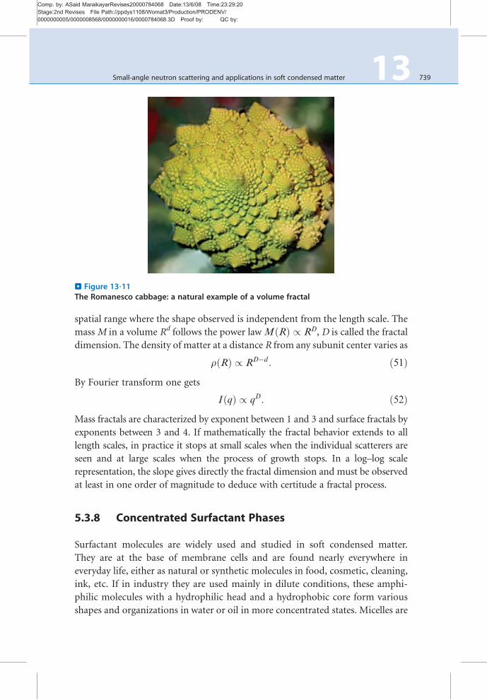
Comp. by: ASaid MaraikayarRevises20000784068 Date:13/6/08 Time:23:29:20Stage:2nd Revises File Path://ppdys1108/Womat3/Production/PRODENV/0000000005/0000008568/0000000016/0000784068.3D Proof by: QC by:
spatial range where the shape observed is independent from the length scale. The
massM in a volume Rd follows the power lawM Rð Þ / RD, D is called the fractal
dimension. The density of matter at a distance R from any subunit center varies as
r Rð Þ / RD�d : ð51ÞBy Fourier transform one gets
I qð Þ / qD: ð52ÞMass fractals are characterized by exponent between 1 and 3 and surface fractals by
exponents between 3 and 4. If mathematically the fractal behavior extends to all
length scales, in practice it stops at small scales when the individual scatterers are
seen and at large scales when the process of growth stops. In a log–log scale
representation, the slope gives directly the fractal dimension and must be observed
at least in one order of magnitude to deduce with certitude a fractal process.
5.3.8 Concentrated Surfactant Phases
Surfactant molecules are widely used and studied in soft condensed matter.
They are at the base of membrane cells and are found nearly everywhere in
everyday life, either as natural or synthetic molecules in food, cosmetic, cleaning,
ink, etc. If in industry they are used mainly in dilute conditions, these amphi-
philic molecules with a hydrophilic head and a hydrophobic core form various
shapes and organizations in water or oil in more concentrated states. Micelles are
. Figure 13‐11The Romanesco cabbage: a natural example of a volume fractal
Small-angle neutron scattering and applications in soft condensed matter 13 739

Comp. by: ASaid MaraikayarRevises20000784068 Date:13/6/08 Time:23:29:21Stage:2nd Revises File Path://ppdys1108/Womat3/Production/PRODENV/0000000005/0000008568/0000000016/0000784068.3D Proof by: QC by:
generally formed at low concentrations. At higher concentrations, or in presence
of salt or by varying the temperature, lamellar, sponge, cubic, or hexagonal phases
are formed. All of these phases give typical patterns, where the form factor is
modulated by the structure factor. In concentrated and well-ordered systems
several Bragg peaks can be measured (see for example, > Figure 13‐13). Fromtheir shape and size, the bending modulus and the rigidity of membranes can be
extracted. For interested readers the following articles and lectures are recom-
mended [45, 46].
5.3.9 Case of Polymers
SANS experiments have greatly contributed to a deeper understanding of the
phase behavior and the structure of polymer melts and solutions. Please refer to
the articles published in this book from G. Berry (vol I, chap 2), C. Giacomeli and
R. Borsali (vol I, chap 3), S. Pederson (vol I, cahp 4), Y. Nakamaru/Norisuye
(vol I, chap 5), I. Hamley & V. Castelletto (vol II, chap 8).
5.3.10 Case of Interfaces
We consider a two-phase system. At large q vectors, the interface is observed at a
small scale. Now if the scattering vector is much larger than the characteristic
curvature of the interfaces, they appear flat and the intensity is proportional to
the total surface area S, independently of the shape of the two phases.
The so-called Porod limit (1951) says that for a sharp interface (in the
normal direction but smooth in any parallel direction) the intensity decreases
as q�4 at large q as
S ¼ 1
2p Dr2ð Þ limq!1 I qð Þq4; ð53Þ
where S is the specific area, i.e, the surface developed by the interface per unit
volume in m2/m3.
Assuming a spherical geometry of the particles, the radius can be deduced as:
R ¼ 3FS
: ð54Þ
In the case of particles of typical size R, measuring in the Porod limit means that
the q-range has to be extended up to q value around qR = 10.
A precise determination of the specific area is closely related to the precision
of the absolute scaling. The equation allows one to determine the size of very large
particles up to the order of micrometers.
740 13 Small-angle neutron scattering and applications in soft condensed matter

Comp. by: ASaid MaraikayarRevises20000784068 Date:13/6/08 Time:23:29:21Stage:2nd Revises File Path://ppdys1108/Womat3/Production/PRODENV/0000000005/0000008568/0000000016/0000784068.3D Proof by: QC by:
An example of an application is the measurement of the droplet size in the
spontaneous emulsion formed by the well-known beverage ‘‘Pastis’’ [50]. The
emulsion is formed by anethol droplets in a continuous medium of water and
ethanol. The radius of droplets is of the order of micrometers and increases
with time and temperature. Even on D22, the complete form factor is not
accessible by SANS. Only the last part of the form factor, decreasing as q�4 is
viewed and from this discrepancy it is possible to deduce the radii of the particles.
The porod law has been used to analyze data from mesoporous materials (or
cement), which develop a large interface with closed pores not accessible with
other techniques (as gaseous absorption, for example). Other applications con-
cern pores in alumine [51], surfactant phases [52], gels [53], or emulsions [54].
Correction of the Porod limit becomes necessary when the modulus of the
scattering vector is of the same order as the surface curvature (surface roughness).
Different corrections are detailed in [55].
The different form factors (sphere, hollow sphere, ellipsoid, cylinder, and
disk) are illustrated in > Figure 13‐12a and b. The calculation is done for radius
or length of 150 A and layer thickness of 20 A, in order to compare for identical
parameters the variation of the scattering curves induced by the different shapes.
The ellipsoidal shape is calculated for R = 150 A and e = 3. For a more realistic
representation, the form factors are smeared by a log-normal polydispersity
function, as will be explained in the next section. The log–log representation
puts clearly into evidence different regimes. At low q, for qR < 1, the scattering
curves reach a plateau and are in the so-called ‘‘Guinier’’ regime. Then the first
oscillation is related to the larger dimension of the scatterers (outer radius,
cylinder length, etc). At intermediary range, the double logarithmic representa-
tion appears as a linear slope which is related to the aggregate shape:
q−1 slope: 1D object like rigid fibers.
q−2 slope: 2D object or locally planar, as for example, membrane, flat
colloidal particle.
At high q, the minimum of the oscillation is related to the lowest dimension
of the objects (vesicle bilayer, disk thickness, etc.), followed by a q−4 slope,
characteristic of the interface between the objects and the solvent.
5.4 Indirect Fourier Transform Method
The following method has been developed by O. Glatter. The details of calculation
are explained in journal articles [56] and in a book of lecture notes [57]. In this
approach, there is no hypothesis a priori on the size, shape, and polydispersity of
the scattered objects. It consists of an inverse Fourier transformation of the
Small-angle neutron scattering and applications in soft condensed matter 13 741

Comp. by: ASaid MaraikayarRevises20000784068 Date:13/6/08 Time:23:29:21Stage:2nd Revises File Path://ppdys1108/Womat3/Production/PRODENV/0000000005/0000008568/0000000016/0000784068.3D Proof by: QC by:
experimental scattering curves which yields the pair distance distribution
function p(r). The PDDF gives information of the structure in the real space
and needs to be compared with calculated models, as spheres, cylinders, etc.
It is also possible to construct amodel based on an analytical form for the objects
with complex shapes and inhomogeneous density. The validity of themodel is tested
by calculation of the PDDF and I(q) and comparison with the experimental data.
Every model that can fit within the errors is acceptable. Additional parameters
(obtained with other techniques) will be needed to select the right model.
More recently, the generalized indirect Fourier transform (GIFT) aims to
determine simultaneously the form factor and the structure factor in case of
interacting particles [58]. The pertinent use of the program package requires
training; it is then an extremely powerful tool for SANS data analysis.
. Figure 13‐12Comparison of form factors. Figure 12 (a) sphere (grey) smeared with a function of poly-dispersity (grey), hollow sphere (red); Figure 12 (b) ellipsoid (green), disk (black) andcylinder (red)
742 13 Small-angle neutron scattering and applications in soft condensed matter

Comp. by: ASaid MaraikayarRevises20000784068 Date:13/6/08 Time:23:29:22Stage:2nd Revises File Path://ppdys1108/Womat3/Production/PRODENV/0000000005/0000008568/0000000016/0000784068.3D Proof by: QC by:
Ab initio analysis of particle shape and domain structure programs has been
developed by D. Svergun as well. The approach based on IFT is explained in detail
in [59]. The powerful algorithms are used in soft condensed matter but also for
biological samples, as for example, to refine the configuration of proteins in
solutions.
5.5 Structure Factors of Colloids
A detailed lecture on interacting colloidal suspensions can be found in [60]. S(q)
is related to the pair correlation function g(r), which describes the local order of
the scatterers, i.e., the probability of finding a particle at a given distance from
another one. g(r) depends on the interaction potential.
g rð Þ ¼ e�V rð Þ
kBT ; ð55Þwhere V(r) is the mean field potential. In case of relatively dilute systems,
V(r) = U(r), the interaction pair potential.
Assuming that N > >1, the structure factor can be written as
S qð Þ ¼ 1þN
V
ðV
g rð Þ � 1ð Þe�iqrdr: ð56Þ
Or in case of isotropic interactions (56) becomes
S qð Þ ¼ 1þ 4pN
V
ðV
g rð Þ � 1ð Þr2 sin qrqr
dr: ð57Þ
Typically, the structure factor is a dimensionless oscillatory function that tends to
unity at high q and equals 1 for dilute solutions. The first maximum at q0 is
related to the distance between the nearest neighbors by 2p=q0. The experimental
structure factors can be obtained by measuring the absolute intensity at two
particle concentrations and by dividing the scattering at the highest concentra-
tion by the one at lowest concentration, in dilute condition. The resulting curve
can be then compared with existing models, trying different pair potential.
Attractive interactions or biphasic samples induce an increase of the intensity at
low q, whereas a decrease of the intensity is the signature of repulsive interactions.
In > Figure 13‐13 an example of aggregation and attractive interaction in lamellar
phase is presented. The lamellar La phase is made by dilution in D2O of AOT, an
anionic surfactant with C12E4, a nonionic surfactant (molar surfactant ratio 1:1).
For a total volume fraction of surfactant of 24%, micelles and La are in osmotic
equilibrium, the sample is slightly turbid and a q �3 upturn is observed at low q.
As soon as the single-phase regime is reached, the low q intensity strongly
Small-angle neutron scattering and applications in soft condensed matter 13 743

Comp. by: ASaid MaraikayarRevises20000784068 Date:13/6/08 Time:23:29:22Stage:2nd Revises File Path://ppdys1108/Womat3/Production/PRODENV/0000000005/0000008568/0000000016/0000784068.3D Proof by: QC by:
decreases. On the other hand, in > Figure 13‐14, the lowering of the low q
intensity is due to the repulsive interaction between charged micelles. The red
curve represents the fitted form factor and the green one is the experimental
structure factor.
. Figure 13‐14Scattering from AOT micelles,F = 1%. ((◊) Experimental points; (▬) Best-fit obtained usingthe form factor of ellipsoid (48), R = 15.7 A, ε = 1.15; (▬) Experimental structure factorobtained by dividing the experimental scattering form by the fitted form factor. Thelowering of the intensity traduces repulsive interactions and the peak position is relatedto the mean distance between micelles
. Figure 13‐13Lamellar phases made by mixing charged (AOT) and uncharged (C12E4) surfactant mole-cules [28]. The molar ratio between AOT and C12E4 is. F is the total volume fraction ofsurfactant in D2O. (◊) F = 24%, (◊) F = 30%. The strong increase of the intensity as a q�3
slope is characteristic from a biphasic sample
744 13 Small-angle neutron scattering and applications in soft condensed matter
Comp. by: ASaid MaraikayarRevises20000784068 Date:13/6/08 Time:23:29:24Stage:2nd Revises File Path://ppdys1108/Womat3/Production/PRODENV/0000000005/0000008568/0000000016/0000784068.3D Proof by: QC by:
Most of the expressions are calculated in the frame of statistical mechanics
and liquid state theory for particles with spherical symmetry and interacting
with a symmetric potential. The pair correlation function g(r) is calculated by
means of the Ornstein–Zernike integral equations with an additional equation
known as the closure equation to describe the pair potential of the system under
investigation.
The wide variety of colloids yields to very different kind of interactions from
hard sphere to long-range soft potentials. There are only few cases where an
analytical expression exists. For all the others, numerical calculations need to be
performed.
For hard-sphere systems, the expression is calculated with the Perkus–Yevick
approximation for the closure relation. The system is fully described by the hard
sphere radius and volume (RSH and FSH) [61].
A widely used analytic expression for charged colloids in a repulsive
screened Coulomb potential has been given by Hayter and Penfold in 1981,
where the OZ equation is solved in the Mean Spherical Approximation theory
(MSA) [62]. The equations are mainly valid in the case of relatively high colloid
concentrations. In 1982, the model has been extended to dilute systems. The new
closure equation is known as the ‘‘Rescaled Mean Spherical Approximation’’
(RMSA) [63].
The model has been successfully applied for charged micelles or colloids. The
variable parameters are the ionic strength (cs), the volume fraction (F), the colloidcharge (s), and the radius (R). Some of these parameters are known from
the sample preparation (cs, F). In many cases, the radius can be extracted
from the form factor. Then structure factor fitting allows one to estimate the
rate of counter-ion dissociation or the screening length, for example. Important
progresses in the understanding of counter-ion role have been so realized and
compared to behavior described by the Hofmeister series.
6 Instrument Resolution and Polydispersity
In the latter chapter, ideal form factors have been presented. However, in most of
the cases, these form factors do not fit the experimental data as well as expected.
Instrument resolution and polydispersity of the scatterers have to be introduced
in the model [64, 65]. Here, the effect of instrumental resolution and polydisper-
sity will be compared.
To illustrate the effects, the model of a spherical shell is used: the outer radius
R1 is fixed at 220 A and layer thickness at 20 A (45). Dr is set at 1 so that P(0) = 1.
A background of 10�3 is added to cut the very deep oscillations at large q (down
Small-angle neutron scattering and applications in soft condensed matter 13 745
Comp. by: ASaid MaraikayarRevises20000784068 Date:13/6/08 Time:23:29:25Stage:2nd Revises File Path://ppdys1108/Womat3/Production/PRODENV/0000000005/0000008568/0000000016/0000784068.3D Proof by: QC by:
to 10�8), to reduce the amplitude of the intensity axis and to see better the
differences between the simulations.
The resolution is the uncertainty of the measured q value and indicates the
possibility to resolve sharp features such as oscillations or Bragg peaks. As shown
below, Dq/q depends partially on the wavelength spread, which is quite different
between time-of-flight and steady-state instruments. The following considers
only the latter kind of instruments. Resolution calculation for time-of-flight
spectrometers is detailed in [66].
The smearing of the ideal scattered intensity has three factors: the finite size
of the incident beam, the wavelength resolution, and the pixel size on the detector
[65]. Only the first two points will be considered since the pixel size (max
10 � 10 mm2) has a negligible effect.
The q-resolution at a given qmay bewritten according to a Taylor expansion as:
Dq ¼ �qdll
� �þ 4p
l
� �cos yDy: ð58Þ
Hence,
Dq2 ¼ q2dll
� �2
þ 4pl
� �2
cos2 yDy2 ¼ Dq2 lð Þ þ Dq2 yð Þ
¼ q21
2ffiffiffiffiffiffiffiffiffiffiffi2 ln 2
p Dll
� �2" #
þ 4pl
� �2
�q2
" #Dy2:
ð59Þ
Dl/l is related to the FWHM (full width at half maximum) value of the triangular
function describing the wavelength distribution by FWHM = l0 (Dl/l). Dy is
related the width of the direct beam (> Figure 13‐15). A detailed description of
Dl/l (δl/l) and Dy is given in Appendix (6.7).
From (59), one can see clearly that Dq2 depends on the wavelength spread
and also on q value. The contribution from Dy is quasi-constant versus q, the
one from l increases with q. At low q (<10�2 A�1), the uncertainly is domi-
nated by the distribution in angle. At large q-values, Dq is due to the wavelength
spread.
The resolution function R(q0, q, Dq) describes the distribution of the q
vectors at a given instrumental configuration. The experimental intensity Iexp is
the real intensity scattered by the sample KcF2(q, ro) (36) smeared by the resolu-
tion function R(q0, q, Dq):
Iexp qð Þ ¼ðq0 þ 1q0 � 1Rðq0; q;DqÞIðq0Þdq0: ð60Þ
Assuming a Gaussian function for the resolution, (60) yields:
746 13 Small-angle neutron scattering and applications in soft condensed matter

Comp. by: ASaid MaraikayarRevises20000784068 Date:13/6/08 Time:23:29:25Stage:2nd Revises File Path://ppdys1108/Womat3/Production/PRODENV/0000000005/0000008568/0000000016/0000784068.3D Proof by: QC by:
Iexp qð Þ ¼ðq0!þ1
q0!�1
1
Dqffiffiffiffiffiffi2p
p exp � q0 � qð Þ22 Dqð Þ2
!IðqÞdq0: ð61Þ
In practice, the range of integration q0 � 1, q0 + 1 is replaced by q0 � a, q0 + a
where a depends on the width of the Gaussian function, i.e., on Dq2. The higherDq2, the larger is the integration range which has to be used. A too small
integration range would yield to an underestimation of the smearing, particularly
at high q, where the function is broader.
6.1 Effect of the Beam Divergence and Size:u Resolution
As shown in (76), Dy varies between 8 � 10�4 and 2.6 � 10�3 rad on D22. These
smearing effects are presented in > Figure 13‐16. In insert, a zoom of the low q
region is presented; the direct beam width is compared to the width of the first
oscillation of the ideal form factor and the resulting smeared curve is drawn. The
direct beam size has a large influence at small angles inducing an intensity
decrease of the plateau and smoothing the first oscillations with a shift of the
minima toward higher q.
6.2 Effect of the l Distribution
In > Figure 13-17, one sees that on such a sample, the effects are most noticeable
for Dl/l > 20%. Above this value, the oscillations vanish. Below 20%, the
. Figure 13‐15Contributions of D l/l (D), Du (+) to the total q-distribution, D q2 (♦). Curves are calculatedfor l = 6 A, D l/l = 10%, and Du = 10�3 rad
Small-angle neutron scattering and applications in soft condensed matter 13 747
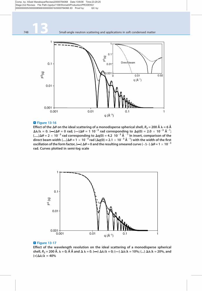
Comp. by: ASaid MaraikayarRevises20000784068 Date:13/6/08 Time:23:29:25Stage:2nd Revises File Path://ppdys1108/Womat3/Production/PRODENV/0000000005/0000008568/0000000016/0000784068.3D Proof by: QC by:
. Figure 13‐16Effect of the Du on the ideal scattering of a monodisperse spherical shell, R2 = 200 A l = 6 ADl/l = 0. (▬)Du = 0 rad; (▬)Du = 1 10�3 rad corresponding to Dq(0) = 2.0 � 10�3 A�1;(.....)Du = 2 � 10�3 rad corresponding to Dq(0) = 4.2 10�3 A �1 In insert, comparison of thedirect beam width (....)Du = 1� 10�3 rad (Dq(0) = 2.1� 10�3 A�1) with the width of the firstoscillation of the form factor, (▬)Du = 0 and the resulting smeared curve (�D�)Du= 1� 10�3
rad. Curves plotted in semi-log scale
. Figure 13‐17Effect of the wavelength resolution on the ideal scattering of a monodisperse sphericalshell, R2 = 200 A. l = 0; A A andD l = 0. (▬)Dl/l = 0; (▬)Dl/l = 10%; (...) Dl/l = 20%, and(+)Dl/l = 40%
748 13 Small-angle neutron scattering and applications in soft condensed matter
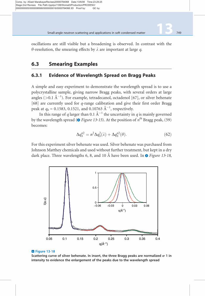
Comp. by: ASaid MaraikayarRevises20000784068 Date:13/6/08 Time:23:29:25Stage:2nd Revises File Path://ppdys1108/Womat3/Production/PRODENV/0000000005/0000008568/0000000016/0000784068.3D Proof by: QC by:
oscillations are still visible but a broadening is observed. In contrast with the
y-resolution, the smearing effects by l are important at large q.
6.3 Smearing Examples
6.3.1 Evidence of Wavelength Spread on Bragg Peaks
A simple and easy experiment to demonstrate the wavelength spread is to use a
polycrystalline sample, giving narrow Bragg peaks, with several orders at large
angles (>0.1 A�1). For example, tetradecanol, octadenol [67], or silver behenate
[68] are currently used for q-range calibration and give their first order Bragg
peak at qb = 0.1583, 0.1521, and 0.10763 A�1, respectively.
In this range of q larger than 0.1 A�1 the uncertainty in q is mainly governed
by the wavelength spread (> Figure 13‐15). At the position of nth Bragg peak, (59)
becomes:
Dqn2b ¼ n2Dq2b lð Þ þ Dqn2b yð Þ: ð62Þ
For this experiment silver behenate was used. Silver behenate was purchased from
Johnson Matthey chemicals and used without further treatment, but kept in a dry
dark place. Three wavelengths 6, 8, and 10 A have been used. In > Figure 13‐18,
. Figure 13‐18Scattering curve of silver behenate. In insert, the three Bragg peaks are normalized s 1 inintensity to evidence the enlargement of the peaks due to the wavelength spread
Small-angle neutron scattering and applications in soft condensed matter 13 749

Comp. by: ASaid MaraikayarRevises20000784068 Date:13/6/08 Time:23:29:26Stage:2nd Revises File Path://ppdys1108/Womat3/Production/PRODENV/0000000005/0000008568/0000000016/0000784068.3D Proof by: QC by:
the scattering curve obtained at l = 6 A, D = 2 m, and C = 14.4 m is presented.
Three Bragg peaks are visible. In insert, the width of the peaks normalized s 1 in
intensity is compared.
The Bragg peaks are fitted with a Gaussian function given Dqnb� �
expequals to
0.0066, 0.011, 0.017 A�2 for n = 1, 2, and 3, respectively. A full series of
measurements at different wavelengths and collimations and calculation details
are presented in [69].
In powder diffraction, the width of the Bragg peak and the enlargement is
related to the mosaicity. In soft condensed matter for lamellar phases, the Bragg
peak shape is related to bending constant and elasticity of bilayer. The presented
example shows the importance of the knowledge of the instrument resolution for
accurate determination of parameters.
Inversely, a well-known crystal with a very small mosaicity giving sharp
Bragg peaks can be used to determine the wavelength spread.
6.3.2 Importance of the Choice of InstrumentConfigurations
The choice of instrument configuration can strongly affect the data analysis. An
example is given in > Figure 13‐19. Calibrated monodisperse latex particles were
purchased by Aldrich (ref cat 46,169-5, R = 430 A, σ = 0.006, size determined by
. Figure 13‐19Scattering of monodisperse spheres of latex at two configurations. l = 6 A, (D), D = 17.6 mand C = 17.6 m, (◊), D = 5.6 m and C = 5.6 m
750 13 Small-angle neutron scattering and applications in soft condensed matter
Comp. by: ASaid MaraikayarRevises20000784068 Date:13/6/08 Time:23:29:27Stage:2nd Revises File Path://ppdys1108/Womat3/Production/PRODENV/0000000005/0000008568/0000000016/0000784068.3D Proof by: QC by:
TEM measurements by Aldrich) and used as received. The two instrument
configurations used optimize the flux at the sample position: D = 17.6 and
C = 17.6 m for the low angles and D = 5.6 and C = 5.6 m, with a wavelength
l = 6 A. The scattering curves are shifted of a factor of 5 in intensity. The form
factor oscillations are clearly visible in the low q configuration, whereas, they are
totally smeared in the other configuration where only the curve envelop is seen. In
such case, data fitting gives very large uncertainly on the radius, around 40% and
sometimes never converges.
6.4 Polydispersity
Most colloidal suspensions are composed of polydisperse objects. The form
factor of monodisperse particles F2(q,R2) is smeared with the size distribution
function G(R2, r, x), where x is the parameter characterizing the width of the
distribution:
Ipoly q;R2ð Þ ¼ð10
GðR2; r; xÞIðq; r2Þdr: ð63Þ
Gaussian, log-normal functions or Schultz distribution are often used to repre-
sent the size spread, around an average value R2. The normalized expressions
(Ð10
GðrÞdr ¼ 1) are given here; their shapes and principal properties are com-
pared in > Figure 13‐20.
. Figure 13‐20Comparison of the three size distribution laws. R2 = 200 A; Dro = 40 A (gaussian); so = 0.2(log-normal), and Z = 90 (Schultz)
Small-angle neutron scattering and applications in soft condensed matter 13 751

Comp. by: ASaid MaraikayarRevises20000784068 Date:13/6/08 Time:23:29:28Stage:2nd Revises File Path://ppdys1108/Womat3/Production/PRODENV/0000000005/0000008568/0000000016/0000784068.3D Proof by: QC by:
� The Gaussian function is:
GG R2; r;Dr2ð Þ ¼ 1
DR2
ffiffiffiffiffiffi2p
p exp � r� R2ð Þ22DR2
2
!; ð64Þ
where DR2 is the half-width of the Gaussian function for
GG R2;R2 þ DR2ð Þ ¼ GðR2Þ expð�1=2Þ ¼ 0:606. The Gaussian function is
symmetric about its maximum R2.
� The log-normal distribution is equal to:
GLN R2; r;soð Þ ¼ 1
rso
ffiffiffiffiffiffi2p
p exp � 1
2s2o
lnR2
r
� �2 !
; ð65Þ
s0 is the standard mean deviation, related to the half-width by Dr0 = s0r0. Themaximum of the function is found for r ¼ ro exp �s2
o
� �.
� The Schultz distribution is:
GS R2; r;Zð Þ ¼ Zþ1R2
Zþ1
exp �R2rð Þ=G Z þ 1ð Þ; with
G Zð Þ ¼ Ð e�ttZ�1dt; the gamma function:ð66Þ
The root mean square deviation from the mean is s ¼ R2= Z þ 1ð Þ1=2. Themaximum of the curve is found at R ¼ ZR2= Z þ 1ð Þ:
The three functions are plotted in > Figure 13‐20. R2 is fixed at 200 A. For
the log-normal and the Schultz functions, the maximum of the curves are slightly
smaller than R2. The half-widths at GðR2Þ expð�1=2Þare related by:
DR2 Gaussianð Þ ¼ soR2 Log�Normalð Þ ¼ R2= Z þ 1ð Þ1=2ðSchultzÞ: ð67ÞFinally, these three expressions yield very similar numerical values (> Figure 13‐20)and it is certainly not possible to distinguish them by a SANS experiment.
In the following, a log-normal law will be used to illustrate the effects of
polydispersity. The effect of polydispersity on the form factor of a spherical shell
of inner radius of 200 A is illustrated in > Figure 13‐21. It is clearly visible for
s0 > 10%. The oscillations vanish and the minimum of the first oscillation is
shifted to higher q values.
6.5 Instrumental Resolution and Polydispersity
If one compares > Figure 13‐17 and > Figure 13‐21, the effects of polydispersity orinstrument resolution are very similar. Indeed, mathematically, the smearing
752 13 Small-angle neutron scattering and applications in soft condensed matter

Comp. by: ASaid MaraikayarRevises20000784068 Date:13/6/08 Time:23:29:28Stage:2nd Revises File Path://ppdys1108/Womat3/Production/PRODENV/0000000005/0000008568/0000000016/0000784068.3D Proof by: QC by:
equations (61) and (63) are similar. An experimental curve results from the
smearing of the ideal intensity both by the resolution and the polydispersity
functions:
Iexp qo;R2ð Þ ¼ð10
R qo; q0ð Þð10
KcGðR2; r;DR2ÞF2ðr; qÞdr� �
dq0 ð68Þ
As q and R2 are independent variables, (68) is also equal to:
Iexp qo;R2ð Þ ¼ðR!1
R¼0
ðq!þ1
q!�1KcRðqo; qÞGðR2; r;DR2ÞF2ðr; qÞdrdq ð69Þ
Remark: Taking a Gaussian law for the polydispersity, the total resolution func-
tion is symmetrical according to the variables q and r. Thus, the smearing effects
due to Dro or Dqo may be equivalent.
6.6 Conclusion
The contribution of the instrumental resolution to the scattering pattern is a
general question. This knowledge is crucial for the data analysis because instru-
mental resolution and sample polydispersity have similar smearing effects on the
SANS data. Smoothing of the form factor oscillations, broadening of Bragg peaks
or of the maxima are observed. Plotting I(q) versus q in a log–log representation
may show a decrease of the initial slope, due to a smearing by a large direct beam
. Figure 13‐21Effect of the polydispersity on the ideal scattering of a monodisperse spherical shell,R2 = 200 A. (▬) s0 = 0; (▬) s0 = 10%; (....) s0 = 20%
Small-angle neutron scattering and applications in soft condensed matter 13 753

Comp. by: ASaid MaraikayarRevises20000784068 Date:13/6/08 Time:23:29:28Stage:2nd Revises File Path://ppdys1108/Womat3/Production/PRODENV/0000000005/0000008568/0000000016/0000784068.3D Proof by: QC by:
may also be present [64]. As shown with simulation, 20% is the limiting value
above which the smearing effect by the wavelength becomes drastic and yields to a
real change in the scattered pattern.
The choice of collimation is a compromise between the flux and the resolu-
tion that has to be considered for each experiment.
6.7 Appendix: Definition of Du and Dl/l; Comparisonbetween Triangle and Gaussian Functions
In the entire text, Gaussian functions are used to describe the wavelength and
the angular distribution. We define here how the widths Dx0 of the Gaussian
functions are calculated. Dl/l usually given is the FWHM which is different
from Dx0We recall that a Gaussian function centered on xo of half width Dx0 at the
value
Gðx;x0;Dx0Þ ¼ 1ffiffiffiffiffiffi2p
pDx0
exp �1=2ð Þ
is given by:
G x;x0;Dx0ð Þ ¼ 1ffiffiffiffiffiffi2p
pDx0
exp � x� x0ð Þ22Dx20
!: ð70Þ
The FWHM of a Gaussian is
FWHM ¼ 2Dx0ffiffiffiffiffiffiffiffiffiffiffi2 ln 2
p: ð71Þ
6.7.1 Wavelength Distribution
The wavelength distribution is ideally triangular but experiments show that
Gaussian fits give reasonable results and improve the numerical treatment [65].
Dl/l is deduced from the FWHM of the triangular function. It is usually
between 5 and 20% with a neutron velocity selector, a value determined by
time-of-flight measurements. Gaussian and triangular functions are compared
in > Figure 13‐22.A triangular function of unit area, centered on lo of FWHM lo(Dl/l) is
given by:
754 13 Small-angle neutron scattering and applications in soft condensed matter

Comp. by: ASaid MaraikayarRevises20000784068 Date:13/6/08 Time:23:29:28Stage:2nd Revises File Path://ppdys1108/Womat3/Production/PRODENV/0000000005/0000008568/0000000016/0000784068.3D Proof by: QC by:
T lð Þ ¼ 1
l0 Dl=lð Þ½ �2 lþl0 1� Dl=lð Þð Þ
l0 Dl=lð Þ½ �2 ; l l0
T lð Þ ¼ �1
l0 Dl=lð Þ½ �2 lþl0 1þ Dl=lð Þð Þ
l0 Dl=lð Þ½ �2 ; l � l0
ð72Þ
The calculation uses a Gaussian function where the relevant parameter is σl, thehalf width at the value 1ffiffiffiffi
2pp
slexp �1=2ð Þ.
We replace the triangular function by a Gaussian one with the same FWHM.
From (71), one deduces:
sl ¼ l0 Dl=lð Þ2ffiffiffiffiffiffiffiffiffiffiffi2 ln 2
p : ð73Þ
Thus, the relative wavelength spread introduces in (59) is:
dl=lð Þ ¼ Dl=lð Þ2ffiffiffiffiffiffiffiffiffiffiffi2 ln 2
p : ð74Þ
6.7.2 Angular Distribution
The angular distribution Dy is deduced from the width of the direct beam. For
q = 0 y = 0 and (58) is reduced to:
. Figure 13‐22Comparison between triangular and Gaussian functions with the same areas used torepresent the wavelength distribution
Small-angle neutron scattering and applications in soft condensed matter 13 755

Comp. by: ASaid MaraikayarRevises20000784068 Date:13/6/08 Time:23:29:28Stage:2nd Revises File Path://ppdys1108/Womat3/Production/PRODENV/0000000005/0000008568/0000000016/0000784068.3D Proof by: QC by:
Dq 0ð Þ ¼ 4plDy: ð75Þ
On D22, the measurements show that reasonable fits are obtained with a Gauss-
ian function, even if deviation is observed in the tails. In these conditions Dq(0) isequivalent to Dx0 in (70) and one easily deduce Dy with (75).
Example of experimental direct beam shapes for l = 6 A at various collima-
tion distances C are presented in > Figure 13‐23.Dy can also be calculated in a theoretical way from the geometry of the
instrument. It is a function of: source diameter (S1), diameter of the aperture in
front of the sample (S2), collimation (C), and sample-to-detector (D) distances.
Details of calculations are given in [67, 68]. As a crude approximation, Dy can be
estimated with:
Dy ¼ S1=C: ð76Þ
7 Present Future and Perspective
7.1 Recent Developments
The new generation of SANS diffractometers like D22 at the ILL (Institut Laue
Langevin, Grenoble) with very high flux at the sample position (up to 108
neutrons/s/cm2) combined with a large sensitive detector area permit very
short acquisition times of the order of a few hundreds of milliseconds [72].
. Figure 13‐23Shape and size of the direct beam of D22 at l = 6 A for the different possible collimationdistances. Dotted lines are a guide for the eyes
756 13 Small-angle neutron scattering and applications in soft condensed matter

Comp. by: ASaid MaraikayarRevises20000784068 Date:13/6/08 Time:23:29:28Stage:2nd Revises File Path://ppdys1108/Womat3/Production/PRODENV/0000000005/0000008568/0000000016/0000784068.3D Proof by: QC by:
The development of new experiments is closely related to instrument
improvement and development of new sophisticated sample environments.
Great progress has been realized in the detector field and electronics as already
presented in > Section 2. In the last few years, complex environments such as
stopped-flow device, shear apparatus, extruder equipment, and flash light opened
the possibility of new kind of investigations.
The last decade has seen the development of kinetics experiments. By rapid,
one means acquisition of the order of hundred milliseconds in order to reach
the early stages of formation of a sample. Real-time means a movie of the sample,
just after a perturbation (dilution, pH jump, temperature change, application of
a magnetic field, etc.). The knowledge of the early stage of sample formation
can be crucial to understand and act on the equilibrium state. One crucial step
with such experiments is to trigger the acquisition with the experimental
setup to insure the reproducibility of the measurement. Small acquisition times
require repeating several times the experiment and adding data to increase the
statistics.
Real-time experiments carried out with the stopped-flow technique have
allowed the study of intermediary or metastable states during the formation of
vesicles [73–75], or to measure characteristic times for formation and growth
of mesoporous materials [76].
In a recent experiment, the changes of conformation of the Photoactive
Yellow Protein were followed during 1.053 s after illumination by a flash light
[17]. The first acquisition time was only 50 ms, a time competitive with what is
done on SAXS instruments on synchrotron sources. The analysis by IFT has
shown an increase of the radius of gyration corresponding to an opening of the
conformation just after illumination followed by a return to the equilibrium state
within a second.
7.2 Future Developments
7.2.1 Interactive Instrument Control
The future of SANS experiments will require the development of new ‘‘intelli-
gent’’ softwares that will be able not only to control the instrument and to set the
configurations but also to pilot the acquisition. A major question, for example, is
how to optimize the acquisition time by keeping good statistics. Future software
will be able to calculate on line statistics and errors and to stop the acquisition
when given conditions defined by the scientist (for example, a given number
of neutrons) will be reached.
Small-angle neutron scattering and applications in soft condensed matter 13 757

Comp. by: ASaid MaraikayarRevises20000784068 Date:13/6/08 Time:23:29:28Stage:2nd Revises File Path://ppdys1108/Womat3/Production/PRODENV/0000000005/0000008568/0000000016/0000784068.3D Proof by: QC by:
7.2.2 Lenses and Focusing
The limiting factors in neutron experiments are the flux, the smallest scattering
vector (qmin), and the resolution, three parameters that can be linked and simul-
taneously improved if focusing devices would exist. The recent investigations consist
in sets of biconcave lenses installed just before the sample [77]. Very encouraging
results have been obtained as described by Choi et al. [78] with test experiments
carried out on the 30-m SANS instrument at NIST [78]. The authors show the
gain of flux, ofminimum q and resolution after correction of chromatic aberration
due to gravity. Nevertheless, some restrictions must be pointed out [79]. Mainly,
such equipment decreases the instrument flexibility such as it is optimized for
one wavelength and one sample-to-detector distance which must match the
focusing point.
Sets of MgF Compound Refractive Lens (CRL) are available on D22
(obtained from PSI). Installed after the sample position they were used to
magnify the sample. Example are given in [80] obtained with Al CRL.
7.2.3 Ultra Small-Angle Scattering (USANS)
At very low q SANS experiments meet the limits of light scattering experiments.
Micro-size particles can be analyzed by techniques like electronic microscopy,
AFM, light scattering or USAXS but in some cases these techniques are not
applicable (opaque sample for SALS, low contrast, etc.). USANS offers the
possibility to investigate very large structures. Worm-like micelles, microemul-
sions, colloidal crystals, porous material as found in cement or rocks are possible
applications in USANS.
USANS instruments can cover a q-range from 2 10�4 to 5 10�3 A�1. They
operate mainly according two principles. The Bonse–Hart setup consists in
two channel-cut perfect crystals mounted in parallel, one is the monochromator,
the second one is the analyzer and the sample is positioned in between.
The q-dependence of the scattered intensity is measured by rocking the crys-
tals [78]. Bonse–Hart-type instruments exist on PCD at the NIST (USA), on
S18 at the ILL (France), on ECHO at SINQ (Switzerland), on KWS-3 in the
FZ-Julich (Germany), and will also be built in Jaeri the new spallation source
in Japan.
The second possible setup is a pinhole geometry, where the beam is colli-
mated in the two directions by a series of small diaphragms or slits. This geometry
has been selected at the LLB (France) for the instrument ‘‘TPA’’ in commissioning
at the date of this review [83] [84].
758 13 Small-angle neutron scattering and applications in soft condensed matter

Comp. by: ASaid MaraikayarRevises20000784068 Date:13/6/08 Time:23:29:29Stage:2nd Revises File Path://ppdys1108/Womat3/Production/PRODENV/0000000005/0000008568/0000000016/0000784068.3D Proof by: QC by:
One main limiting factor in USANS experiments is the low flux at the sample
position.
Nevertheless the new high flux reactors and spallation sources render the
experiments possible. The use of multiple small beams further focused at
the sample position is an efficient way to increase the flux.
7.2.4 Polarization and SANS
Some SANS spectrometers1 offer now a polarization option opening new possible
fields of research. The polarization has a strong influence on the contrast between
nuclear and magnetic scattering contribution. The incident polarized beam is
produced by a supermirror. Polarization alone can be used as a way to vary the
contrast of the sample. The principle of a ‘‘polarization plus analysis’’ experiment
consists in applying a magnetic field to the sample and to analyze the spin states
before and after the scattering. Complementary to conventional SANS, additional
information magnetization profiles in samples are obtained. Recent outcomes on
ferrofluids are described in [16].
Another application comes from the large spin-dependent scattering length
from 1H. Consequently, polarized SANS can find strong application in soft
condensed matter and biology where hydrogen is a main component. Contrast
variation can be done once again using hydrogen 1H and deuterium 2H which
exhibit strong differences in spin-dependence [82].
Nanotechnologies using magnetism and new biotechnologies will certainly
benefit from polarized SANS, opening new approaches for the sample character-
ization.
7.3 General Conclusion
SANS is a powerful technique to analyze the size, the shape, the intra- and
interstructures of complex systems with typical size ranging from a few nanometres
down to tenths of a micrometer. The lowest flux and the larger beam size compared
to X-ray source is balanced by the unique feature of isotopic substitution which has
been of particular importance in the understanding of biological systems.
In comparison with light or X-ray scattering, small-angle neutron scattering
is a relatively recent technique, still in evolution. Technical progresses are also
closely linked to electronics improvements. Progress in computing permits more
1 PAPOL, LLB, France; SANSPOL, HMI, Germany; SANS-I at SINQ, Switzerland, NG3 30m at
NIST, United States
Small-angle neutron scattering and applications in soft condensed matter 13 759
Comp. by: ASaid MaraikayarRevises20000784068 Date:13/6/08 Time:23:29:29Stage:2nd Revises File Path://ppdys1108/Womat3/Production/PRODENV/0000000005/0000008568/0000000016/0000784068.3D Proof by: QC by:
and more accurate fittings with numerical resolution of nonlinear equations
involved in theoretical models.
SALS, SAXS, and SANS techniques are not in competition but really com-
plementary. Moreover microscopy techniques (in the real space) are often carried
out in parallel to validate the models deduced from scattering experiments.
Reference [41] illustrates nicely the complementarities of freeze-fracture electron
microscopy and SANS.
The increasing number of proposals submitted per year demonstrates the
relevance of this technique. The future developments and the broad field of
research investigated insure a bright future for SANS experiments.
Acknowledgements
I would warmly thank Dr. S King and Dr R. Heenan (ISIS), for the documents
supplied on LOQ. I am grateful to P. Van Esch (ILL, Grenoble) for the technical
explanations on detectors. I am grateful to Ron Ghosh (Institut Laue Langevin)
for discussion on instrument resolution. I would like to thank Bruno Deme for
helpful discussions in perspective and application for USANS instruments.
Thanks to C. Dewhurst for the manuscript reading and comments on data
analysis. I thank R. May for the training on D22 at the ILL and all fruitful
discussions.
References
1. Guinier, A. (1939) Ann. Phys. Paris., 12,
161–237.
2. Guinier, A., Fournet, G. 1955 Small Angle
Scattering of X-Rays. Wiley, New York.
3. Stuhrmann, H.B. (1974) Neutron Small-
angle scattering of biological macromole-
cules in solution. J. Appl. Cryst., 7,
173–178.
4. Stuhrmann, H.B. and Duee, E.D. (1975)
The determination of the scattering den-
sity distribution of polydisperse solutions
by contrast variation: a neutron scatter-
ing study of ferritin. J. Appl. Cryst., 8,
538–542.
5. Ibel, K. and Stuhrmann, H.B. (1975)
J. Mol. Biol., 93, 255–265.
6. http://www.ill.eu/lss/more/world-directory-
of-sans-instruments/ and http://www.
isis.rl.ac.uk/LargeScale/LOQ/other/World_
Directory_of_SANS_Instruments.htm.
7. Glinka, C.J., Barker, J.G., Hammouda, B.,
Krueger, S., Moyer, J.J., and Orts,
W.J. (1998) The 30 m small angle neutron
scattering experiments at the national
institute of standards and technology.
J. Appl. Cryst., 31, 430–445.
8. Heenan, R.K., Penfold, J., King, S.M
(1997) SANS at pulsed neutron sources:
present and future prospects. J. Appl.
Cryst., 30, 1140–1147 (http://www.isis.rl.
ac.uk/largescale/loq/loq.htm).
760 13 Small-angle neutron scattering and applications in soft condensed matter
Comp. by: ASaid MaraikayarRevises20000784068 Date:13/6/08 Time:23:29:31Stage:2nd Revises File Path://ppdys1108/Womat3/Production/PRODENV/0000000005/0000008568/0000000016/0000784068.3D Proof by: QC by:
9. Knoll, G.F. and Wihley J.(1989) Position-
sensitive detection of thermal neutrons.
In Convert, P. and Forsyth, J.B. (ed.),
Radiation Detection and Measurement.
Academic Press, New York.
10. Knoll, G.F. 1989. Radiation Detection and
Measurement, Chap. 7, 2nd ed. Wiley,
New York; P. Lindner, Dead time of the
BF3 detector at D11, ILLTechnical report,
ILL98/LI 12 T (1998).
11. Van Esc, P., Gahl, T., Guerard, B. (2004)
Design criteria for electronics for resistive
charge division in thermal neutron detec-
tion. Nucl. Instr. Meth. Phys., Res. A, 526,
493–500.
12. Van Esch, P. and Millier, F. (2003) Opti-
mal lookup table construction with respect
to efficiency flatness. Rev. Sci. Instrum., 74,
5058–5061.
13. Scherm, R. and Fak, B. (1993). Neutron
and synchrotron radiation for condensed
matter studies. In Baruchel, J. Hodeau,
J.L., Lehmann, M.S., Regnard, J.R., and
Schlenker C. (eds.), Theory, instruments
and methods. Les Editions de physique,
Vol 1, Chap. 5. Springer, Berlin.
14. May, R., Hendriks, J., and Crielaard, W.
(2005) Real-time neutron scattering
investigations of biological signal trans-
duction dynamics. In Proceedings of the
International Symposium on Research Re-
actor and Neutron Science, Daejeon,
Korea, pp 777–781.
15. Bent, J., Hutchings, L.R., Richards, R.W.,
Cough, T., Spares, R., Coates, P.D., Grillo,
I., Harlen, O.G., Read, D.J., Graham, R.S.,
Likhtman, A.E.,Groves, D.J., and Nichol-
son, T.M (2003) Neutron -mapping poly-
mer flow: scattering flow visualization
and molecular theory. T.C.B. McLeish
Sci., 301, 1691–1695 (abstract).
16. Heinemann, A., Wiedenmann, A. (2005)
Insight into the formation of partially
ordered structures in Co-based ferro-
fluids. J. Magn. Magn. Mater., 289,
149–151.
17. Jacrot, B. and Zaccai, G. (1981) Deter-
mination of molecular weight by
neutron scattering.Biopolymers, 20,
2413–2426.
18. Lindner, P. (2000) Water calibration at
D11 verified with polymer samples.
J. Appl. Crystallogr., 33, 807–811.
19. Gosh, R.E, Egelhaaf, S.U., and Rennie,
A.R. (1998) A computing guide for
Small-Angle Scattering Experiments; ILL
report ILL98GH14T. GRASP for Gra-
phical Reduction and analysis SANS pro-
gram for Matlab™ by C. Dewhurst (http://
www.ill.eu/sites/grasp/grasp_main.html).
20. Sears, V.F. (1992) Neutron scattering
lengths and crossed sections. Neutron
News, 3, 26–37.
21. Schelten, J. and Schmatz, W. (1980) Mul-
tiple scattering treatment for small-angle
scattering problems. J. Appl. Crystallogr.,
13, 385–390; Goyal, P.S., King, J.S., and
Summerfield, G.C. (1983) Multiple scat-
tering in small-angle neutron scattering
measurements on polymers. Polymer, 24,
131–134; Berk, N.F. and Hardman-Rhyne,
K.A. (1988) Analysis of SAS data domi-
nated by multiple scattering. J. Appl. Crys-
tallogr., 21, 645–651.
22. Lal, J., Widmaier, J.M., Bastide, J., and
Boue, F. (1994) Determination of an
interpenetrating network structure by
small angle neutron scattering. Macromo-
lecules, 27, 6443–6451.
23. Morfin, I., Ehrburger-Dolle, F., Grillo, I.,
Livet, F., and Bley, F. (2006) ASAXS, SAXS
and SANS investigations of vulcanized
elastomers filled with carbon black. Part
6, 445–452.
24. Brulet, A., Lairez, D., Lapp, A., Cotton, J.P.
(2007) Improvement of data treatment in
small-angle neutron scattering J Appl
Cryst. 40, 165–177.
25. Silas, J.A. and Kaler, E.W. (2003). Effect of
multiple scattering from bicontinuous
microemulsions. J. Colloid Interface Sci.,
257, 291–298.
26. Glatter, O. and Kratky, O. 1982 Small
Angle X-Ray Scattering. Academic Press,
London.
27. Boue, F., Cotton, J.P., Lapp, A., and
Jannink, G. (1994) A direct measurement
of the polyion conformation in aqueous
solutions at different temperatures. Small
angle neutron scattering of PSSNa using
Small-angle neutron scattering and applications in soft condensed matter 13 761

Comp. by: ASaid MaraikayarRevises20000784068 Date:13/6/08 Time:23:29:34Stage:2nd Revises File Path://ppdys1108/Womat3/Production/PRODENV/0000000005/0000008568/0000000016/0000784068.3D Proof by: QC by:
zero average and full contrast. J. Chem.
Phys., 101, 2562–2568; Brulet, A., Boue,
F., Cotton, J.P. (1996) About the experi-
mental determination of the persistence
length of wormlike chains of polystyrene.
J. Phys. II France, 6, 885–891; Spiteri, M.N.,
Boue, F., Lapp, A., and Cotton, J.P. (1996)
Persistence length for a PSSNA Polyion
in semidilute solution as a function of
the ionic strength. Phys. Rev. Lett., 77,
5218–5220.
28. Morfin, I., Lindner, P., and Boue, F. (2004)
Shear–induced concentration fluctua-
tions and form factor changes in polymer
solution in the good-solvent regime. Eur.
Phys. J. E., 15, 41–45.
29. Oberdisse, J. (2007) Current Opinion in
Colloid an Interface Science. Adsorption
grafting on colloidal interfaces studied by
scattering techniques. 12, 3–8.
30. Boue, F., Cousin, F., Gummel, J., Ober-
disse, J., Carrot, G., El Harrack, A.
(2007) Small angle scatteing from soft
matter – application to complex mixed
systems. C.R. Phys 8, 821–844.
31. Balnois, E., Durand-Vidal, S., and Levitz, P.
(2003) Probing the morphology of Lapo-
nite clay colloids by atomic force micros-
copy. Langmuir, 19, 6633–6637.
32. Mourchid, A., Delville, A., Lambard, J.,
Lecolier, E., and Levitz, P. (1995)
Phase diagram of colloidal dispersions
of anisotropic charged particles: equilibri-
um properties, structure and rheology
of laponite suspensions. Langmuir, 11,
1942–1950.
33. Grillo, I. (personal communication).
34. Bates,F.S.,Wignall,G.D., and Koehler,W.C.
(1985) Critical behavior of binary liquid
mixtures of deuterated and protonated
polymer. Phys. Rev. Lett., 55, 2425.
35. Arleth, L. and Pedersen, J.S. (2000)
Scattering vector dependence of the
small-angle scattering from mixtures of
hydrogenated and deuterated organic sol-
vents. J. Appl. Crystallogr., 33, 650–652.
36. Jacrot, J. (1976) The study of bio-
logical structures by neutron scattering
from solution. Rep. Prog. Phys., 39,
911–953.
37. Pedersen J. (1997) Analysis of small-
angle scattering data from colloids and
polymer solutions: modeling and least-
squares fitting. Adv. Colloid Interface Sci.,
70, 171–210.
38. Rayleigh, L. (1911)The Incidence of Light
upon a Transparent Sphere of Dimensions
Comparable with the Wave-Length. Proc.
Royal. Soc. Lodon. Ser. A., 84, 25–38.
39. Dingenouts, N., Selenmeyer, S., Deike, I.,
Roseneldt, S., Ballauf, M., Lindner, P., and
Narayanan, T. (2001) Analysis of thermo-
sensitive core-shell colloids by small-angle
neutron scattering including contrast
variation. Phys. Chem. Chem. Phys., 3,
1169–1174.
40. Sommer, C., Pedersen, J.S., and Garamus,
V.M. (2005) Sructure and interaction of
block copolymermicelles of Brij 700 studied
by combining small-angle X-ray and neu-
tron scattering. Langmuir, 21, 2137–2149.
41. Bumajdad, A., Eastoe, J., Nave, S., Steytler,
D.C., Heenan, R.K., and Grillo, I. (2003)
Compositions of mixed surfactant layers
in microemulsions determined by SANS.
Langmuir, 19, 2560–2567.
42. Fournet, G. (1951) Bull. Soc. Fr. Miner.
Crist., 74, 39–113.
43. Eastoe, J., Rogueda, P., Shariatmadai, D.,
and Heenan, R. (1996) Micelles of asym-
metric chain catanionic surfactants. Col-
loids surf. A Physicochem. Eng. Asp., 117,
215–225.
44. Zemb, T., Dubois, M., Deme, B.,
and Gulik-Krzywicki, T. (1999) Self-
assembly of flat nanodiscs in salt-free
catanionic surfactant solutions. Science,
283, 816–819.
45. Coulombeau, H., Testard, F., Zemb, T.,
and Larpent, C. (2004) Effect of recog-
nized and unrecognized salt on the
self-assembly of new thermosensitive
metal-chelating surfactants. Langmuir,
20, 4840–4850.
46. Simmons, B., Agarwal, V., McPherson, G.,
John, V., and Bose, A. (2002) Small angle
neutron scattering study of mixed AOT +
lecithin reverse micelles. Langmuir, 18,
8345–8349.
47. Jung, M., Robinson, B.H., Steytler, D.C.,
German, A.L, and Heenan, R.K. (2002)
Polymerization of styrene in DODAB
vesicles: a small-angle neutron scattering
study. Langmuir, 18, 2873–2879.
762 13 Small-angle neutron scattering and applications in soft condensed matter
Comp. by: ASaid MaraikayarRevises20000784068 Date:13/6/08 Time:23:29:39Stage:2nd Revises File Path://ppdys1108/Womat3/Production/PRODENV/0000000005/0000008568/0000000016/0000784068.3D Proof by: QC by:
48. Caille, A. (1972) X-ray scattering by
smectic-A crystals. C. R. Hebd. Acad. Sci.
Paris B., 274, 891–893.
49. Nallet, F., Laversanne, R., and Roux, D.
(1993) Modelling X-ray or neutron scat-
tering spectra of lyotropic lamellar phases.
Interplay between form and structure fac-
tors. J Phys. II, 3, 487–502.
50. Grillo, I. (2003) Small angle neutron scat-
tering of a world-wide known emulsion:
Le Pastis Colloids surf. A Physicochem. Eng.
Asp., 225, 153–160.
51. Marchal, D., Bourdillon, C., and Deme
Small-Angle, B. (2003) Neutron scattering
by highly oriented hybrid bilayer mem-
branes confined in anisotropic porous
alumine. Langmuir, 26, 8313–8320.
52. Deme, B. and Zemb, T. (2000) Measure-
ment of sugar depletion from uncharged
lamellar phases by SANS contrast varia-
tion. J. Appl. Cryst., 33, 569–573.
53. Kanaya, T., Ohkura, M., Takeshita, H.,
Kaji, K., Furusaka, M., Yamaoka, H., and
Wignall, G.D. (1995) Gelation process of
poly(vinyl alcohol) as studied by small-
angle neutron and light scattering.Macro-
molecules, 28, 3168. The Netherlands,
Amsterdam.
54. Steytler, D.C., Dowding, P.J., Robinson,
B.H., Hague, J.D., Rennie, J.H.S., Leng,
C.A., Eastoe, J., and Heenan R.K. (1998)
Characterization of water-in-oil microe-
mulsions formed in silicone oils. Lang-
muir, 14 3517–3523.
55. Auvray, L. and Auroy, P. (1991) Neutron,
X-Ray and light scattering: introduction
to an investigative tool for colloidal and
polymeric systems. In Lindner, P. and
Zemb, T. (eds.), North Holland delta se-
ries. III. Scattering by interfaces: variation
on Porod’s law. The Netherlands, North
Holland delta series, Amsterdam.
56. Glatter, O. (1977) Data evaluation in
small-angle scattering, calculation of
radial electron density distribution by
means of indirect fourier transformation.
Acta Phys. Austriaca, 47, 83–102;
Glatter, O. (1977) New method for evalu-
ation of small angle scattering data.
J. Appl. Crystallogr., 10, 415–421; Glatter,
O. (1980) Determination of particle size
distribution functions from small-angle
scattering by means of the indirect trans-
formation method. J. Appl. Crystallogr.,
13, 7–11.
57. Lindner, P., and Zemb, T. (eds.) (2002)
Neutron, X-rays and light: scattering
methods applied to soft condensed mat-
ter, chaps. 4 and 5. Elsevier. The Nether-
lands, Amsterdam.
58. Weyerich, B., Brunner-Popela, J., and
Glatter, O. (1999) Small-angle scattering
of interacting particles. II. Generalized in-
direct Fourier transformation under con-
sideration of the effective structure factor
for polydisperse systems. J. Appl. Crystal-
logr., 32, 197–209.
59. Svergun, D.I. and Koch, M.H.J., (2003)
Small-angle scattering studies of
biological macromolecules in solution.
Rep. Prog. Phys., 66, 1735–1782.
60. Lindner, P. and Zemb, T. (eds.) (2002)
Neutron, X-rays and Light: Scattering
Methods Applied to Soft Condensed Mat-
ter, chapters 14. Elsevier.
61. Percus, J.K and Yevick, G.J. (1958) Analy-
sis of classical mechanics by means of
collective coordinates. Phys Rev., 1, 1–13.
62. Hayter, J.B. and Penfold, J. (1981) An
analytic structure factor for macroion
solutions. Mol. Phys., 42, 109–118.
63. Hansen, J.P. and Hayter, J.B. (1982) A
rescaled MSA structure factor for dilute
charged colloidal dispersions. Mol. Phys.,
46, 651–656.
64. Schmatz, W., Springer, T., Schelten, J., and
Ibel, K. (1974) Neutron small-angle scat-
tering - Experimental techniques and
applications. J. Appl. Cryst., 7, 96–116;
Wignall, G.D., Christen, D.K., and
Ramakrishnan V. (1988) Instrumental reso-
lution affects in small-angle neutron scat-
tering J. Appl. Cryst., 21, 438–451; Milder,
D.F.R. (1990) Design optimization of a
small-angle neutron scattering spectrom-
eter. Nucl. Instrum. Methods Phys. Res. A,
290, 259–262.
65. Pedersen, J.S., Posselt, D., and Mortensen,
K. (1990) Analytical treatment of the res-
olution function for small-angle scatter-
ing. J. Appl. Crystallogr. 23, 321–333.
66. Mildner, D.F.R., Carpenter, J.M., and
Worcester, D.L. (1986) Measurement and
calculation of resolution of time-of-flight
Small-angle neutron scattering and applications in soft condensed matter 13 763
Comp. by: ASaid MaraikayarRevises20000784068 Date:13/6/08 Time:23:29:44Stage:2nd Revises File Path://ppdys1108/Womat3/Production/PRODENV/0000000005/0000008568/0000000016/0000784068.3D Proof by: QC by:
small-angle neutron scattering J. Appl.
Crystallogr., 19, 311–319.
67. Ne, F., Grillo, I., Tache, O., and Zemb,
T.H. (2000) De l’intensite brute a l’inten-
site absolue, calibration d’une camera
Guinier-Mering. J. Phys. IV., 10, 403–413.
68. Huang, T.C., Toraya, H., Blanton, T.N.,
and Wu, Y (1993) J. Appl. Crystallogr.,
26, 180–184.
69. Grillo, I. (2001) ILL technical Report
ILL01GR08T, Effect of instrumental reso-
lution and polydispersity on ideal form
factor in Small Angle Neutron Scattering.
70. Mildner, B.F.R. and Carpenter, J.M.
(1984) Optimization of the experimental
resolution for small-angle scattering.
J. Appl.Crystallogr., 17, 249–256.
71. Lairez, D. (1999) Resolution d’un spectro-
metre de diffusion de neutrons aux petits
angles. J. Phys. IV France, 9, 67–81.
72. http://www.ill.ev/dzz/documentation/.
73. Egelhaaf, S.U., Olsson, U., and Schurte-
berger, P. (2000) Time resolved SANS for
surfactant phase transitions. Physica B,
276–278, 326–329.
74. Grillo, I., Kats, E.I., and Muratov, A.R.
(2003) Formation and growth of anionic
vesicles followed by small-angle neutron
scattering. Langmuir, 19, 4573–4581.
75. Gradzielski, M., Grillo, I., and Narayanan,
T. (2004) Dynamics of structural transi-
tions in amphiphilic systems monitored
by scattering techniques. Prog. Colloid.
Polym. Sci., 129, 32–39.
76. Ne, F., Testard, F., Zemb, T., et al. (2003)
How does ZrO2/surfactant mesophase
nucleate? Formation mechanism. Lang-
muir, 19, 8503–8510.
77. Williams, R.E. and Michael Rowe J.
(2002) Developments in neutron beam
devices and in advanced cold source for
the NIST research reactor. Physica B, 311,
117–122.
78. Choi, S.M., Barker, J.G., Glinka, C.J.,
Cheng, Y.T., and Gammel, P.L. (2000)
Focusing cold neutrons with multiple
biconcave lenses for small-angle neutron
scattering. J. Appl. Crystallogr., 33,
793–796.
79. Littrell, K.C. (2004) A comparison of dif-
ferent methods for improving flux and
resolution on SANS instrument. Nucl.
Instrum. Methods Phys. Res. A, 529, 22–27.
80. Dewhurst, C.D., Anderson, I., and
Beguiristain, R. (2001) ILL Annual Re-
port. In Cicognani, G. and Vettier, C.
(ed.), Imaging with a Neutron Lens.
81. Bonse, U. and Hart, M. Small-Angle
X-Ray Scattering. In Brumberger, H.
(ed.), Gordon and Breach, New York,
pp 121.
82. Stuhrmann, H.B., Van der Brandt, B.,
Hautle, P., Konter, J.A., Ninikoski, T.O.,
Schmitt, M., Willumeit, R. Zhao, J., and
Mango, S. (1997) Polarized neutron scat-
tering from polarized nuclei near para-
magnetic centres. J. Appl. Crystallogr., 30,
839–843.
83. Desert, S., Thevenot, J., Oberdisse, A.,
Brulet, J. (2007) The new very-small-
angle neutron scattering spectrometer at
Laboratoire Leon Brillouin. J. Appl. Cryst.
40, S471–S473.
84. Brulet, A., Thevenot, V., Lairez, D.,
Lecommandoux, S., Agut, W., Armes, S.P.,
Du, L.Z., Desert, S. (2008) Toward a new
lower limit for the minimum scattering
vector on the very small angle neutron
scattering spectrometer at Laboratoire
Leon Brillouin. J. Appl. Cryst. 41, 161–166.
764 13 Small-angle neutron scattering and applications in soft condensed matter
List of Contributors
BALLAUFF, MATTHIAS
University of Beyreuth
Bayreuth
Germany
BERRY, GUY C.
Carnegie Mellon University
Pittsburgh, PA
USA
BORSALI, REDOUANE
CERMAV, CNRS-UPR 5301 and Joseph
Fourier University
Grenoble Cedex
France
BURCHARD, WALTHER
Albert-Ludwig-University of Freiburg
Freiburg
Germany
CASTELLETTO, VALERIA
University of Leeds
Leeds
UK
CHOI, YOUNG-WOOK
Hanyang University
Seoul
South Korea
CHU, BENJAMIN
Stony Brook University
Stony Brook, NY
USA
COHEN-BOUHACINA, TOURIA
University of Bordeaux 1
Pessac Cedex
France
DAS, RHIJU
Stanford University
Stanford, CA
USA
DEFFIEUX, ALAIN
University of Bordeaux I
Pessac, Cedex
France
DOBEREINER, HANS-GUNTHER
Columbia University
New York, NY
USA
DONIACH, SEBASTIAN
Stanford University
Stanford, CA
USA

DOUCET, GARRETT J.
Louisiana State University
Baton Rouge, LA
USA
DUXIN, NICOLAS
McGill University
Montreal, QC
Canada
EDWIN, NADIA
Louisiana State University
Baton Rouge, LA
USA
EISENBERG, ADI
McGill University
Montreal, QC
Canada
ESAKI, SIEJI
Osaka University
Osaka
Japan
GIACOMELLI, CRISTIANO
University of Caxias do Sul (UCS)
Caxias do Sul
Brazil
GRILLO, ISABELLE
Institute Laue Langevin
Grenoble Cedex
France
GRUBEL, GERHARD
Hasylab/DESY
Hamburg
Germany
HAMLEY, IAN
University of Leeds
Leeds, UK
HASHIMOTO, TAKEJI
Kyoto University
Katsura, Kyoto
Japan
HAUSTEIN, ELKE
Biotec TU Dresden
Dresden
Germany
HOLM, CHRISTIAN
Max-Planck-Institute for Polymer
Research
Mainz
Germany
ISHII, YOSHIHARU
Osaka University
Osaka
Japan
KOZUKA, JUN
Japan Science and Technology Agency
Osaka
Japan
LAZZARONI, ROBERTO
University of Mons-Hainaut
Mons
Belgium
MAALI, ABDELHAMID
University of Bordeaux I
Pessac, Cedex
France
xii List of contributors

MADSEN, ANDERS
European Synchrotron Radiation Facility
Grenoble Cedex
France
NAKAMURA, YO
Kyoto University
Kyoto
Japan
NARAYANAN, T.
European Synchrotron Radiation Facility
Grenoble Cedex
France
NOIREZ, LAURENCE
Laboratory Leon Brillouin
Cedex
France
NORISUYE, TAKASHI
Osaka University
Osaka
Japan
PECORA, ROBERT
Stanford University
Stanford, CA
USA
PEDERSEN, JAN SKOV
University of Aarhus
Aarhus
Denmark
QIU, JIANHONG
Louisiana State University
Baton Rouge, LA
USA
REITER, GUNTER
Institute of Chemistry of Surfaces and
Interfaces
Cedex
France
RICKGAUER, JOHN PETER
University of California – San Diego
San Diego, CA
USA
ROBERT, AYMERIC
European Synchrotron Radiation Facility
Grenoble Cedex
France
RUSSO, PAUL S.
Louisiana State University
Baton Rouge, LA
USA
SCHAPPACHER, MICHEL
University of Bordeaux 1
Pessac Cedex
France
SCHARTL, WOLFGANG
Johannes-Gutenberg-University Mainz
Mainz
Germany
SCHWILLE, PETRA
Biotec TU Dresden
Dresden
Germany
SHIBAYAMA, MITSUHIRO
University of Tokyo
Tokyo
Japan
List of contributors xiii

SMITH, DOUGLAS E.
University of California – San Diego
San Diego, CA
USA
SOHN, DAEWON
Hanyang University
Seoul
South Korea
TIRRELL, MATTHEW
University of California – Santa Barbara
Santa Barbara, CA
USA
TOOMEY, RYAN
University of South Florida
Tampa, FL
USA
VIVILLE, PASCAL
University of Mons-Hainaut
Mons
Belgium
YANAGIDA, TOSHIO
Osaka University
Osaka
Japan
xiv List of contributors