predictive qsar tools to aid in early process development

Predictive QSAR tools to aid in early process

development of monoclonal antibodies

John Micael Andreas Karlberg

Published work submitted to Newcastle University for the degree of

Doctor of Philosophy in the School of Engineering

November 2019

i

Abstract

Monoclonal antibodies (mAbs) have become one of the fastest growing markets for diagnostic

and therapeutic treatments over the last 30 years with a global sales revenue around $89 billion

reported in 2017. A popular framework widely used in pharmaceutical industries for designing

manufacturing processes for mAbs is Quality by Design (QbD) due to providing a structured

and systematic approach in investigation and screening process parameters that might influence

the product quality. However, due to the large number of product quality attributes (CQAs) and

process parameters that exist in an mAb process platform, extensive investigation is needed to

characterise their impact on the product quality which makes the process development costly

and time consuming. There is thus an urgent need for methods and tools that can be used for

early risk-based selection of critical product properties and process factors to reduce the number

of potential factors that have to be investigated, thereby aiding in speeding up the process

development and reduce costs.

In this study, a framework for predictive model development based on Quantitative Structure-

Activity Relationship (QSAR) modelling was developed to link structural features and

properties of mAbs to Hydrophobic Interaction Chromatography (HIC) retention times and

expressed mAb yield from HEK cells. Model development was based on a structured approach

for incremental model refinement and evaluation that aided in increasing model performance

until becoming acceptable in accordance to the OECD guidelines for QSAR models.

The resulting models showed that it was possible to predict HIC retention times of mAbs based

on their inherent structure. Further improvements of the models are suggested due to

performance being adequate but not sufficient for implementation as a risk assessment tool in

QbD. However, the described methodology and workflow has been proven to work for retention

time prediction in a HIC column and is therefore likely to be applicable to other purification

columns.

iii

List of publications resulting from this research

Karlberg, M., von Stosch, M. and Glassey, J., 2018. “Exploiting mAb structure characteristics

for a directed QbD implementation in early process development.” Critical reviews in

biotechnology, 38(6), pp.957-970

Kizhedath, A., Karlberg, M. and Glassey, J., 2019. “Cross interaction chromatography based

QSAR model for early stage screening to facilitate enhanced developability of monoclonal

antibody therapeutics”. Biotechnology journal, Accepted

Karlberg, M., Kizhedath, A., Glassey, J., 2019. “QSAR model for Hydrophobic Interaction

Chromatography behaviour from primary sequence of monoclonal antibodies”. Biotechnology

Journal, Submitted

Karlberg, M., de Souza, J., Kizhedath, A., Bronowska, A, Glassey, J., 2019. “QSAR model for

Hydrophobic Interaction Chromatography behaviour from 3D structure of monoclonal

antibodies”. Biotechnology Journal, Submitted

List of conference contributions

Karlberg, M, von Stosch, M, McCreath, G, Glassey, J. “Early Bioprocess development using

PAT approaches”, ESBES, Sep 2016, Dublin, Ireland

Karlberg, M, “Exploiting mAb structure characteristics for a directed QbD implementation in

process development”, XIII BioProcess UK”, Nov 2016, Newcastle, UK

Karlberg, M, Kizhedath, A., von Stosch, M, Wilkinson, S, Glassey J. “Exploiting mAb structure

characteristics for rapid screening and a directed QbD implementation in process

development”, ACS Biot 253rd meeting, Apr 2017, San Francisco, USA

Karlberg, M, von Stosch, M, Glassey, J. “Exploiting mAb structure characteristics for a directed

QbD implementation in process development”, WCCE ECAB, Oct 2017, Barcelona, Spain

Karlberg, M and Glassey, J. “Exploiting MAB structure characteristics for a directed QbD

implementation in process development”, ESBES, Sep 2018, Lisbon, Portugal

v

Acknowledgements

Many people have supported me during the past three years, and I have greatly enjoyed working

with all of them. Especially, I would like to thank my main supervisor and friend, Jarka Glassey

for pushing me to always do better and for providing encouragement to keep on going. Without

this, I would not have learned as much as I now know today for which I am truly grateful. I

would like to thank secondary supervisor Agnieszka Bronowska for showing me the cool world

of Molecular Dynamics and the endless potential it holds for use in process development of

biologics. I also want to thank Joao Victor de Souza Cunha for taking the time in teaching me

the theory and application of Molecular Dynamics which added great value to the project. I also

want to thank my former supervisor Moritz von Stosch for all the fruitful discussion on

multivariate data analysis.

In the city of Newcastle and at Newcastle University, I would like to thank my friends Arathi,

Andre, Ana, Sylvester and Joao, who made every day an adventure. I truly enjoyed coming to

university every day.

From Fujifilm Diosynth in Billingham, UK, I would also like to thank the people who supported

and helped me during my secondment. I truly appreciate the industrial insight and fruitful

discussion that they provided as this clarified the problem statement of this project and

encouraged me to continue research on this topic.

I would also like to thank my family and friends in Sweden for their continued support and

encouragement when writing up this thesis. During the three years of the project I had the

pleasure and honour of becoming godfather to my beloved nephew Gabriel and niece Maja for

which I will definitely tell tall tales and stories about my great adventure across the seas.

This project received funding from the European Union’s Horizon 2020 Research and

Innovation Programme under the Marie Skłodowska-Curie Grant Agreement No 643056

(Biorapid project).

vii

Table of Contents

Abstract ...................................................................................................................................... i

List of publications resulting from this research .................................................................. iii

List of conference contributions ............................................................................................. iii

Acknowledgements ................................................................................................................... v

List of Figures ......................................................................................................................... xv

List of Tables ......................................................................................................................... xxv

Abbreviations ....................................................................................................................... xxix

Nomenclature ..................................................................................................................... xxxiii

Introduction .............................................................................................................................. 1

Thesis structure ....................................................................................................................... 2

Chapter 1: Literature Review .............................................................................................. 2

Chapter 2: Modelling Development and Assessment ......................................................... 2

Chapter 3: Primary Sequence-based Descriptors ................................................................ 2

Chapter 4: Impact of mAb isotypes and species origins on primary sequence-based

descriptors ........................................................................................................................... 3

Chapter 5: QSAR model development: Primary sequence-based descriptors .................... 3

Chapter 6: 3D Structure Descriptors ................................................................................... 3

Chapter 7: QSAR model development: 3D Structure Descriptors ...................................... 3

Chapter 8: Conclusion and Future Perspectives .................................................................. 3

Chapter 1 Literature review .................................................................................................... 5

1.1 Antibody Market ............................................................................................................... 5

1.2 State of the Art in mAb manufacturing............................................................................. 7

1.2.1 Implementation of QbD ............................................................................................. 8

1.2.2 Challenges in QbD implementation ......................................................................... 14

1.2.3 Current Focus and Improvements in Process Development .................................... 15

1.3 Quantitative Structure-Activity Relationship ................................................................. 19

viii

1.3.1 Descriptor generation ............................................................................................... 19

1.3.2 QSAR for protein behaviour prediction .................................................................. 22

1.4 Towards mAb process development by bridging QbD and QSAR................................ 22

1.5 Scope of this study ......................................................................................................... 24

1.6 Summary ........................................................................................................................ 26

Chapter 2 Modelling Development and Assessment ........................................................... 29

2.1 Matrix, vector and index notations ................................................................................. 29

2.1.1 Independent data ...................................................................................................... 29

2.1.2 Dependent data ........................................................................................................ 30

2.2 Exploratory Data Analysis ............................................................................................. 31

2.2.1 Principal Component Analysis ................................................................................ 31

2.2.1.1 Theory ............................................................................................................... 31

2.2.1.2 Applicability of PCA in this research ............................................................... 34

2.3 Classification .................................................................................................................. 35

2.3.1 Partial Least Square – Discriminant Analysis ......................................................... 36

2.3.1.1 Theory ............................................................................................................... 36

2.3.1.2 Applicability of PLS-DA in this research ......................................................... 39

2.3.2 Support Vector Machines for Classification ............................................................ 40

2.3.2.1 Theory ............................................................................................................... 41

2.3.2.2 Soft Margin ....................................................................................................... 43

2.3.2.3 Kernel Trick for non-linearity ........................................................................... 45

2.3.2.4 Applicability of SVC in this research ............................................................... 46

2.3.3 Multiclass Classification Problems.......................................................................... 47

2.4 Regression ...................................................................................................................... 48

2.4.1 Partial Least Square Regression .............................................................................. 48

2.4.1.1 Theory ............................................................................................................... 49

2.4.1.2 Applicability of PLS in this research ................................................................ 52

2.4.2 Support Vector Machines for Regression ................................................................ 53

2.4.2.1 Theory ............................................................................................................... 53

2.4.2.2 Applicability of SVR in this research ............................................................... 55

2.5 Cross Validation ............................................................................................................. 56

2.5.1 Generalisation Error ................................................................................................. 57

ix

2.5.2 Selection of Model Complexity ............................................................................... 60

2.6 Model Validation Metrics ............................................................................................... 61

2.6.1 Regression Metrics ................................................................................................... 61

2.6.2 Classification Metrics ............................................................................................... 62

2.6.3 Y-Randomisation ..................................................................................................... 65

2.7 Data Pre-treatment .......................................................................................................... 66

2.8 Variable Reduction ......................................................................................................... 67

2.9 Variable Selection ........................................................................................................... 67

2.9.1 Recursive Partial Least Squares ............................................................................... 67

2.9.2 Genetic Algorithm .................................................................................................... 68

2.9.3 Sparse L1-SVR ......................................................................................................... 69

2.10 Summary ....................................................................................................................... 70

Chapter 3 Primary sequence-based descriptors .................................................................. 73

3.1 The Antibody Structure .................................................................................................. 73

3.1.1 The Fab region structure and function ..................................................................... 74

3.1.2 The Fc region structure and function ....................................................................... 74

3.1.3 Sequence variability in constant domains ................................................................ 75

3.1.4 Disulphide bonds ...................................................................................................... 76

3.1.5 Sequence variation from humanisation .................................................................... 78

3.2 Descriptor generation ...................................................................................................... 79

3.2.1 Software based descriptors ....................................................................................... 79

3.2.2 Amino acid scale descriptors.................................................................................... 83

3.3 Sequence preparation and conversion ............................................................................. 84

3.3.1 Domain based ........................................................................................................... 85

3.3.2 Window based .......................................................................................................... 85

3.3.3 Substructure Based ................................................................................................... 86

3.3.4 Running Sum based .................................................................................................. 87

3.3.5 Single Amino Acid based ......................................................................................... 87

3.3.6 Differences between strategies ................................................................................. 88

3.4 Summary ......................................................................................................................... 90

x

Chapter 4 Impact of mAb isotypes and species origins on primary sequence-based

descriptors............................................................................................................................... 93

4.1 Material and Methods ..................................................................................................... 93

4.1.1 Sequence gathering .................................................................................................. 93

4.1.2 Descriptor Generation .............................................................................................. 94

4.1.3 Modelling Methods .................................................................................................. 94

4.1.3.1 Principal Component Analysis.......................................................................... 94

4.1.3.2 Partial Least Square Discriminant Analysis ...................................................... 94

4.1.3.3 Support Vector Machines for Classification ..................................................... 94

4.1.4 Data Curation and Pre-treatment ............................................................................. 95

4.1.5 Model Training and Validation ............................................................................... 95

4.1.5.1 Structured data splitting .................................................................................... 95

4.1.5.2 Cross Validation ................................................................................................ 95

4.1.5.3 Model Validation .............................................................................................. 96

4.2 Results and Discussion ................................................................................................... 96

4.2.1 Domain based selection of descriptors .................................................................... 96

4.2.2 Exploration of HC Isotypes ..................................................................................... 97

4.2.3 Exploration of LC Isotypes .................................................................................... 100

4.2.4 Exploration of species origin ................................................................................. 100

4.2.5 Species origin classification .................................................................................. 101

4.3 Summary ...................................................................................................................... 104

Chapter 5 QSAR Model development: Primary sequence-based descriptors ............... 107

5.1 Material and Methods ................................................................................................... 107

5.1.1 Response Data ....................................................................................................... 107

5.1.1.1 mAb expression and extraction ....................................................................... 108

5.1.1.2 HIC .................................................................................................................. 108

5.1.1.3 Exclusion of samples ...................................................................................... 109

5.1.2 Descriptor Data Generation ................................................................................... 109

5.1.3 Modelling Methods ................................................................................................ 109

5.1.3.1 PLS .................................................................................................................. 109

5.1.3.2 SVR ................................................................................................................. 109

5.1.4 Model Training and Validation ............................................................................. 110

5.1.4.1 Structured data splitting .................................................................................. 110

xi

5.1.4.2 Cross-Validation scheme ................................................................................. 110

5.1.4.3 Model Validation ............................................................................................. 110

5.1.4.4 Y-Randomisation ............................................................................................. 110

5.1.5 Descriptor reduction and selection ......................................................................... 111

5.1.5.1 V-WSP ............................................................................................................. 112

5.1.5.2 rPLS ................................................................................................................. 113

5.1.5.3 GA ................................................................................................................... 113

5.1.5.4 LASSO ............................................................................................................ 113

5.1.6 Model Benchmarking ............................................................................................. 114

5.1.7 Statistical testing .................................................................................................... 115

5.1.7.1 Parametric methods ......................................................................................... 116

5.1.7.2 Non-parametric methods ................................................................................. 116

5.1.7.3 Multiple comparison ........................................................................................ 116

5.2 Results and discussion .................................................................................................. 117

5.2.1 Selection of samples for model development ........................................................ 117

5.2.2 Impact of species origin ......................................................................................... 119

5.2.2.1 Behaviour of species origins in PLS models ................................................... 119

5.2.2.2 Significance of species origins ........................................................................ 123

5.2.3 HIC model development on humanised samples ................................................... 123

5.2.4 mAb yield model development on humanised samples ......................................... 128

5.3 Summary ....................................................................................................................... 130

Chapter 6 3D Structure Descriptors ................................................................................... 133

6.1 Structure Generation ..................................................................................................... 133

6.1.1 Background on in silico methods ........................................................................... 134

6.2 Homology Modelling .................................................................................................... 134

6.2.1 Antibody Template Selection ................................................................................. 137

6.2.2 Pairwise Cysteine Distance Restraints ................................................................... 138

6.2.3 Model Assessment.................................................................................................. 139

6.2.4 Structure considerations ......................................................................................... 140

6.3 Protein dynamics ........................................................................................................... 141

6.3.1 Describing the system dynamics ............................................................................ 142

6.4 Molecular Dynamics ..................................................................................................... 144

xii

6.4.1 Force Fields ........................................................................................................... 146

6.4.2 The MD Algorithm and Time Integration ............................................................. 152

6.4.3 Periodic Boundary Conditions ............................................................................... 154

6.4.4 Thermodynamic macro and microstates ................................................................ 156

6.4.5 GROMACS System Equilibration ......................................................................... 158

6.5 Modifications of protein structure and solvent ............................................................. 160

6.5.1 Co-solvent preparation ........................................................................................... 160

6.5.2 Modification of residue protonation states ............................................................ 163

6.6 Descriptor Generation .................................................................................................. 165

6.6.1 Time frame selection ............................................................................................. 167

6.6.2 Descriptor software and calculations ..................................................................... 168

6.6.3 Descriptor resolution ............................................................................................. 170

6.7 Summary ...................................................................................................................... 171

Chapter 7 QSAR Model Development: 3D Structure Descriptors .................................. 173

7.1 Material and Methods ................................................................................................... 174

7.1.1 Response Data ....................................................................................................... 174

7.1.2 Descriptor Data Generation ................................................................................... 174

7.1.3 Modelling Methods ................................................................................................ 175

7.1.3.1 PCA ................................................................................................................. 175

7.1.3.2 PLS-DA ........................................................................................................... 175

7.1.3.3 SVC ................................................................................................................. 175

7.1.3.4 PLS .................................................................................................................. 175

7.1.3.5 SVR ................................................................................................................. 176

7.1.4 Data curation and pre-treatment ............................................................................ 176

7.1.5 Model Training and Validation ............................................................................. 176

7.1.5.1 Structured data splitting .................................................................................. 176

7.1.5.2 Cross-Validation scheme ................................................................................ 176

7.1.5.3 Model Validation ............................................................................................ 176

7.1.5.4 Y-Randomisation ............................................................................................ 177

7.1.6 Variable reduction and Selection ........................................................................... 177

7.1.6.1 V-WSP ............................................................................................................ 177

7.1.6.2 rPLS ................................................................................................................ 178

7.1.6.3 GA ................................................................................................................... 178

xiii

7.1.6.4 LASSO ............................................................................................................ 178

7.2 Results and Discussion ................................................................................................. 178

7.2.1 Analysis of protein dynamics ................................................................................. 178

7.2.2 Impact of the light chain isotypes .......................................................................... 181

7.2.3 Impact of species origin ......................................................................................... 183

7.2.4 HIC model development on IgG1-kappa samples ................................................. 185

7.2.5 mAb yield model development on IgG1-kappa samples ....................................... 189

7.2.6 Comparison to primary sequence-based models .................................................... 191

7.3 Summary ....................................................................................................................... 192

Chapter 8 Conclusions and Future Work .......................................................................... 195

8.1 Descriptors .................................................................................................................... 196

8.1.1 Suggestion for Improvements ................................................................................ 197

8.2 Sample Selection ........................................................................................................... 198


8.3 Model Development and Assessment ........................................................................... 199


8.4 Summary ....................................................................................................................... 202

References.............................................................................................................................. 205

Appendix A ............................................................................................................................ 237

A.1 Marketed mAbs ............................................................................................................ 237

A.2 IMGT mAbs ................................................................................................................. 240

A.3 Predictive Modelling mAbs .......................................................................................... 247

Appendix B ............................................................................................................................ 253

B.1 MATLAB Scripts ......................................................................................................... 253

B.2 GROMACS Parameters ................................................................................................ 255

Appendix C ............................................................................................................................ 261

C.1 Chapter 4 Modelling Results ........................................................................................ 261


xiv


Appendix D ........................................................................................................................... 277

D.1 Eigenvectors and Eigenvalues ..................................................................................... 277

D.2 Singular Value Decomposition .................................................................................... 279

D.3 Lagrange Multipliers in SVC ....................................................................................... 280

xv

List of Figures

Figure 1.1. Approval and market trends of mAbs. (a) History of approved mAbs by EMA

(blue) and FDA (green) annually (bars) and cumulative (lines) as well as

approved biosimilars by either EMA, FDA or both shown in red. (b) History

of market revenue from 2008 to 2018 (green bars) and prognosis of the

expected market revenue between 2019 and 2022 (red bars) where an

optimistic revenue prognosis has been included (grey bars). Based on market

data from EvaluatePharma® (2018) and Grilo and Mantalaris (2019). .................. 6

Figure 1.2. General outline of the QbD methodology. The process design space is shown

as the dashed box where the effects of process parameters and raw material

input (blue box) on the product quality is characterised. Steps highlighted in

red indicate risk assessment of either product quality attributes, process

parameters or raw materials. The green box indicates availability of clinical

data which can be used to better define the QTPP (adapted from Chatterjee

(2012)). .................................................................................................................... 8

Figure 1.3. Overview of the parallelisation between the clinical trials and the process

development (adapted from Li and Easton (2018) as well as Mercier et al.

(2013)) ................................................................................................................... 12

Figure 1.4. General overview of platform-oriented purification of mAbs. The black boxes

represent chromatographic columns and steps that are always included,

whereas the red boxes represent chromatographic polishing steps that change

depending on the behaviour and quality requirements of the mAb. The order

of the second polishing step and the viral filtration can be switched (adapted

from Shukla et al. (2017)) . .................................................................................... 16

Figure 1.5. Proposed integration of QSAR into QbD where the upper half illustrates the

simplified framework of QbD (blue) and the lower half illustrates a simplified

version of the QSAR framework (black). Transfer of characterisation data

from previous mAb processes can be used directly for model development

using QSAR. Depending on the purpose of the developed QSAR model, it

can be used to directly aid in assessing CQAs or provide insight into PPs and

ranges. .................................................................................................................... 24

xvi

Figure 2.1. Overview and critical steps of data decomposition with PCA in two

dimensions. (a) The raw data is first (b) pre-treated by mean centring the

samples around the origin. (c) Linear combinations of the original variables,

x1 and x2, known as eigenvectors are then calculated where the first

eigenvector, v1 (red), lies in the direction of the greatest data variation and

the second eigenvector, v2 (blue), in the direction of the second greatest data

variation. (d) Final transformation of samples to the PC1 (red line) and PC2

(blue line) axes where each sample is represented by its individual scores

(adapted from O'Malley (2008)) ........................................................................... 34

Figure 2.2. The structure of the response vector Y in a binary classification problem used

in PLS-DA. (a) Dummy variables are used to construct Y and assign class

memberships of samples to either C1 (blue) and C2 (red). (b) Example

predictions from the PLS regression. .................................................................... 37

Figure 2.3. Probability distributions used in Bayes theorem. (a) Examples of the

likelihood distributions of y belonging to class C1 (blue line) and C2 (red line)

centred around zero and one, respectively. The distribution of y (dashed grey

line) with equal samples sizes, PC1 = PC2 = 0.5. (b) The posterior

probabilities of a sample belonging to either to class C1 (blue line) or C2 (red

line) based on y with the decision boundary, d (dashed black line) (adapted

from Pérez et al. (2009)). ...................................................................................... 39

Figure 2.4. SVC placement of the decision boundary (black line) generated from selected

samples that act as support vectors (black circles) which maximises class

discrimination in a problem that is (a) linearly separable and (b) not linearly

separable. The SVC constraints for separating positive and negative class

samples are shown as the red dashed line and blue dashed line, respectively

(adapted from Boser et al. (1992)) ........................................................................ 41

Figure 2.5. Transformation with a non-linear mapping function, φx, from a two-

dimensional variable space to a three-dimensional feature space where the

positive samples (red) become linearly separable from the negative samples

(blue). .................................................................................................................... 45

xvii

Figure 2.6. Classification strategies for multiclass problems with (a) One versus One and

(b) One versus Rest. Decision boundaries are shown as dashed black lines

(adapted from Statnikov et al. (2004)). .................................................................. 48

Figure 2.7. Correlation of scores of the first component from the decomposed X and Y

blocks with PLS. .................................................................................................... 50

Figure 2.8. Placement of regression tube in SVR defined by two constraints (red and blue

dashed lines) that encompasses the majority of the samples and where

samples falling outside of the tube are penalised by the slack variables ξi* and

ξi. Support vectors are indicated as the filled black circles and the green vector

perpendicular to the black regression line represents the support vector

weights, ω (adapted from Drucker et al. (1997)). ................................................. 54

Figure 2.9. Splitting of all available samples in a data set into a calibration set for training

(dark box) and a test set for model validation (red box) (adapted from Raschka

(2018)). .................................................................................................................. 57

Figure 2.10. (a) Behaviour of the test or generalisation error (red line) compared to the

fitted model error (black line) with regards to increasing model complexity.

(b) Decomposition of the generalisation error (red line) into the two

components model variance (green line) and model bias (blue line) (adapted

from Hastie et al. (2009a)). .................................................................................... 58

Figure 2.11. K-fold cross-validation resampling of the calibration samples for model

training (adapted from Raschka (2018)). ............................................................... 61

Figure 2.12. Representation of a confusion matrix as an overview of model performance

for (a) multiple classes of (b) two classes (adapted from Fawcett (2006)). .......... 63

Figure 2.13. ROC curve development for two classes. The number of TP, TN, FP and FN

changes depending on to the placement of the threshold which is less drastic

in a problem with (a) well-separated class distributions compared to a

problem with (b) overlapping class distributions. ROC curves from (b) well

separated class distributions and (d) overlapping class distributions where the

black dashed line represents the AUC value of 0.5 (adapted from Marini

(2017)). .................................................................................................................. 65

xviii

Figure 2.14. The effect of pre-treatment on variables on a data set. (a) Raw or untreated

data set. (b) Mean centred data set. (c) Mean centred and scaled data set

(adapted from van den Berg et al. (2006)). ........................................................... 66

Figure 2.15. Crossover of variables between two parent chromosomes A and B resulting

in two new variable permutations in the form of child C and D. The red line

indicates the crossover site which is selected at random by the GA method

(adapted from Pandey et al. (2014)). ..................................................................... 68

Figure 2.16. Comparison of solutions for (a) L2-norm and (b) L1-norm. The red ellipses

represent the error between the predicted and measured responses in the

samples set while the green areas represent the allowed solutions for ω

(adapted from Zhu et al. (2004)). .......................................................................... 70

Figure 3.1. General structure of an IgG1 antibody. (a) Front view of the antibody showing

the separate domains of the heavy chain (VH, CH1, Hinge, CH2 and CH3)

depicted in blue as well as the separate domains of the light chain (VL and CL)

depicted in orange. (b) Side view of the antibody structure with the two

glycan structures highlighted with a red circle. Each glycan connects to

Asn297 of each heavy chain (adapted from Vidarsson et al. (2014)). .................. 74

Figure 3.2. Heavy and light chain isotypes and allotypes. (a) Sequence alignment of the

constant domains CH1, Hinge, CH2 and CH3 in the heavy chain showing all

structural differences between the isotypes IgG1, IgG2 and IgG4. Sequence

numbering follows the EU numbering scheme and positions marked as bold,

underlined and coloured red are positions with varying residues originating

from different allotypes. Positions marked with red boxes highlight residues

that are important in the Fc effector function (b) Comparison of the common

allotypes with the positions in the primary sequence isolated to illustrate the

varying residues based on given alleles. Allele names containing IGHG1 refer

to IgG1, IGHG2 to IgG2 and IGHG4 to IgG4 (c) Sequence alignment of the

constant domain CL in the light chain illustrating the structural differences

between the isotypes kappa and lambda. Positions with varying residues in

the sequences of known allotypes are marked as bold, underlined and

coloured red. (d) Comparison of most common isotypes of the CL domain

where only positions with varying residues are illustrated. Allele names

xix

containing IGKC refer to the kappa isotypes while allele names containing

IGLC refer to the lambda isotypes (adapted from Lefranc and Lefranc

(2012)). .................................................................................................................. 77

Figure 3.3. Representation of antibody modification where orange domains are expressed

domains from the animal model and blue domains are expressed from human

genome. Level of modification is presented in increasing order from fully

animal (a), to chimeric (b), to humanised (c) and finally to fully human (d)

(adapted from Absolute Antibody (2018)). ........................................................... 78

Figure 3.4. Descriptor generation workflow. a) Sequence alignment and splitting was

performed to prepare sequence fragments and amino acids for descriptor

generation of the five data blocks: Domain based, Window based,

Substructure based, Running Sum based and Single Amino Acid based. b)

Descriptors for the Domain based, Window based and Substructure based

approaches were generated from the prepared fragments with ProtDCal,

eMBOSS PEPSTAT and amino acid scales. As for the Single Amino Acid

based and Running Sum based, only the amino acids scales were used to

generate the descriptors (dashed red line). ............................................................ 81

Figure 3.5. Breakdown of the variable domains into the smaller framework (FR) and CDR

substructures. Conserved cysteines are represented as a yellow line while

conserved aromatic residues are represented as blue lines (adapted from

Lefranc et al. (2003)). ............................................................................................ 86

Figure 4.1. Descriptor selection based on the structural origin of investigated response for

(a) heavy chain isotypes, (b) light chain isotypes and (c) species origin.

Descriptors from the mAb domains used in structural exploration are coloured

red while excluded domains are coloured grey in the three presented cases. ........ 96

Figure 4.2. PCA exploration of VH, CH1, CH2 and CH3 descriptors from PSD1. (a) Score

plot of the first two principal components (PCs). The isotypes IgG1 are

coloured red, IgG2 coloured green and IgG4 coloured blue. (b) Loadings of

the first PC. (c) Loadings of the second PC. ......................................................... 99

xx

Figure 4.3. PCA analysis of VL and CL descriptors from the PSD1 descriptor set. (a) Score

plot of the first two principal components (PCs). The isotype kappa is

coloured red and lambda is coloured green. (b) Loadings of the first PC. ......... 100

Figure 4.4. PCA scores of the first and second principal components (PCs) from VH and

VL domain descriptors of PSD1. (a) chimeric (red), human (green) and

humanised (blue) samples. (b) I LC isotypes kappa (red) and lambda (green) .. 101

Figure 4.5. ROC curves and AUC for chimeric (red line), human (green line) and

humanised (blue line) samples developed on prediction data from the cross-

validation of PSD3 in (a) PLS-DA and (b) SVC. The black dashed line

represents the AUC value of 0.5 where no discrimination between classes can

be made. .............................................................................................................. 104

Figure 5.1. General summary of mAbs in the dataset from Jain et al. (2017) according to

(a) the light chain isotypes, (b) species origins and (c) clinical phase

distribution. ......................................................................................................... 108

Figure 5.2. Overview and placement consideration of the V-WSP algorithm in regards to

the data splitting and the variable selection (VS). (a) Placement of V-WSP

reduction prior to structured sample splitting results in a biased selection of

descriptors due to influence from all samples. (b) Structured splitting

performed before V-WSP reduction results in an unbiased selection of

descriptors due to being independent from the test set samples. Vertical

arrows represent selection of descriptors in the test set to match the calibration

set. ....................................................................................................................... 112

Figure 5.3. Sequential model development and evaluation for investigation of changes in

performance with descriptor reduction and selection methods. Three models

are developed on 1) all available descriptors, 2) the V-WSP reduced

descriptor set and 3) the descriptor set after supervised variable selection

(VS). .................................................................................................................... 115

Figure 5.4. Decision tree for statistical testing of response data based on normality and

number of available levels for the investigated factor. ....................................... 116

Figure 5.5. PLS error for prediction of HIC retention times in the calibration (blue line)

and the cross-validation (red line) with regards to the number of latent

xxi

variables developed from the V-WSP reduced descriptor sets of (a) PSD1, (b)

PSD2, (c) PSD3 and (d) PSD4. ........................................................................... 120

Figure 5.6. Impact of species on PLS models developed using the HIC retention times as

the modelled response where chimeric samples are coloured red, human

samples in green and humanised in blue. PLS Influence plots for PSD1 (a),

PSD2 (c), PSD3 (e) and PSD4 (g). PLS scores (T) for the individual samples

for PSD1 (b), PSD2 (d), PSD3 (f) and PSD4 (h). ............................................... 122

Figure 5.7. HIC retention time predictions of 45 IgG1-kappa humanised mAbs with PLS

model (3 LVs) developed on the PSD1 descriptor set after reduction with V-

WSP and selection with GA. (a) Measured versus predicted plot with

calibration (grey) and test (red) samples. (b) Predicted and measured HIC

retention times of test set samples. ...................................................................... 125

Figure 5.8. Regression coefficients of the PLS model (3 LVs) developed on the PSD1

descriptor set after reduction with V-WSP and selection with GA. .................... 125

Figure 5.9. mAb yield predictions of 55 IgG1-kappa humanised and chimeric mAbs with

PLS model (3 LVs) developed on the PSD4 descriptor set after reduction with

V-WSP and selection with GA. (a) Measured versus predicted plot with

calibration (grey) and test (red) samples. (b) Prediction and measured HIC

retention times of test set samples. ...................................................................... 129

Figure 6.1. Distance restraint of cysteines in adalimumab generated. Structure coloured

as orange depicts the light chain and structure coloured as blue depicts the

heavy chain (a) Homology model without added distance restraints to the

interchain cysteines. (b) Homology model with restraint between the

interchain cysteines. ............................................................................................. 139

Figure 6.2. DOPE score for generated model (orange line) and template (green line) for

the light chain (a) and heavy chain (b) for the aligned residues. Positions of

CDR loops regions are marked by name and arrows in both the heavy and

light chain. ........................................................................................................... 140

Figure 6.3. Potential dynamics of a protein. (a) A simplified energy landscape for an

arbitrary protein. Environmental changes can drastically change the

landscape as shown in the shift from the green line to the orange line with a

xxii

different conformation occupying the energy minima. (b) The time scale

needed to observe local as well as global conformational changes in a protein

(adapted from Henzler-Wildman and Kern (2007) and Adcock and

McCammon (2006)). ........................................................................................... 142

Figure 6.4. The relationship between the system size and possible simulation times for

QM, atomistic and coarse-grained simulations. Loss of information is

inevitable when moving to simplified estimation of the system such as

atomistic and coarse-grained representation which are illustrated by the green

and orange graphs, respectively (adapted from Kmiecik et al. (2016)). ............. 145

Figure 6.5. (a) The bonded interactions originating from bond stretching, angle bending

and bond torsion (rotation). (b) The non-bonded interactions originating from

electrostatic and van der Waals potentials (adapted from Allen (2004) and

Leach (2001b)). ................................................................................................... 147

Figure 6.6. Potential energy of bonded interactions. (a) An approximation of the potential

energy in the bond stretching using Hooke’s law as a function of the distance

between two bonded atoms. (b) The potential energy from angle bending as

a function of the angle between two connecting bonds and approximated with

Hooke’s law. (c) Approximation of the potential energy from bond torsion as

a function of the bond angle. Highest potential is observed in eclipsed

conformation and lowest in staggered conformation (adapted from the

GROMACS manual 5.1.4). ................................................................................. 149

Figure 6.7. Potential energy of non-bonded interactions. (a) The electric potential as a

function of distance between two charged points. (b) The van der Waals

potential approximated with Lennard-Jones potential (green line) as a

function of the distance between two non-bonded atoms. Consists of one

repulsion (orange dashed line) and one attraction (orange full line) component

(adapted from the GROMACS manual 5.1.4). ................................................... 151

Figure 6.8. Four steps of the global MD algorithm. Step 1) Positions and initial velocities

are assigned and a force field chosen. Step 2) Calculation of resulting forces

on all atoms in the system. Step 3) Updates the positions and velocities of all

atoms in the system. Step 4) Saves specified information to a log file (adapted

from the GROMACS User Manual 5.1.4). ......................................................... 153

xxiii

Figure 6.9. The application of the periodic boundary condition in a simulation. (a)

Movement of particles out of the simulation box will enter the opposite. (b)

Depicts the cut-off radius for long-range interactions as the dashed red circle

and the importance of choosing a proper box size in order to avoid overlap

and self-interaction (adapted from González (2011)). ......................................... 155

Figure 6.10. A system coupled to a virtual heating bath illustrating the heat exchange

between the heat bath and the system of interest (adapted from Ghiringhelli

(2014)). ................................................................................................................ 158

Figure 6.11. Workflows for modification of environment and protein structure. (a)

Preparation workflow of a co-solvent compound from a SMILE structure to

resulting coordinate and topology files that can be used in GROMACS with

the use of USCF Chimera and ACPYPE. (b) PDB structure modification of

pH dependent residues with htmd ProteinPrepare from Acellera. Residue

protonation states were predicted with PROPKA3.1 according to a target pH

and then assigned with the PDB2PQR function. A structural optimization is

performed to relax the structure prior to conversion to a PDB format ................ 162

Figure 6.12. Impact of pH on the electrostatic surface of adalimumab Fab fragment. At a

pH of 2 the surface is predominately positively charged (blue) and shift to

become more negatively charged (red) with increasing pH. The figure was

generated from surface renderings using USCF Chimera (version 1.13). ........... 164

Figure 6.13. Outline of protein structure prediction, protein dynamics simulation and

descriptor generation. Structure was predicted with MODELLER and

distance restraints for cysteines involved in disulphide bridges. MD

simulations were performed with GROMACS where environmental factors

such as pH and co-solvents could be added. Descriptor generation was

performed with ProtDCal and TAE calculations which modified with

individual residue SASA values obtained from GROMACS. ............................. 166

Figure 6.14. MD simulation result for adalimumab. (a) The conformational change of

adalimumab evolving over time in the production run. (b) The average

fluctuations of the individual residues in the light chain between t=5 ns and

t=50 ns. (c) The average fluctuations of the individual residues in the heavy

chain between t=5 ns and t=50 ns. ....................................................................... 168

xxiv

Figure 7.1. RMSD plots of GROMACS simulations where (a) mAbs have reached

conformational stability and (b) mAbs that have not reached conformational

stability. ............................................................................................................... 179

Figure 7.2. Displacement of the VH domain (blue arrow) in the simulation of eldelumab

from the domains original position captured at (a) 25 ns to its new placement

captured at (b) 35 ns. The heavy chain is coloured blue while the light chain

is coloured red. .................................................................................................... 180

Figure 7.3. PCA score plots of the first two components calculated from the light chain

descriptors from MSD1 (a), MSD2 (b) and MSD3 (c) where kappa and

lambda samples are coloured red and green, respectively. ................................. 182

Figure 7.4. Predictions of HIC retention times with PLS-GA model developed on the

MSD3 descriptor set (LVs = 9). (a) Measured versus predicted plot with

calibration samples in black and test set samples in red. (b) Measured (black)

and predicted (red) values of test set samples. .................................................... 187

Figure 7.5. Predictions of mAb yield with a PLS-GA model developed on the MSD3

descriptor set (LVs = 3). (a) Measured versus predicted plot with calibration

samples (black) and test set samples (red). (b) Measured (black) and predicted

(red) values of test set samples. ........................................................................... 190

xxv

List of Tables

Table 1.1. List of potential CQAs related to common structural variants in mAbs (adapted

from Alt et al. (2016)). ........................................................................................... 10

Table 1.2. Overview of the clinical phases for an mAb candidate with their corresponding

research goals and scope (adapted from the ICH E8 guidelines). ......................... 13

Table 3.1. Summary of structural differences of the constant domains in the heavy and

light chains (adapted from Lefranc et al. (2005) and Liu and May (2012)) .......... 76

Table 3.2. List of generated descriptors from ProtDCal and EMBOSS Pepstats. The stars

in the second and third columns represent which software was used for

generation of each descriptor. ................................................................................ 80

Table 3.3. Amino acid groups available in ProtDCal. RTR, BSR and AHR are based on

common residues found in secondary structure. ALR, ARM, NPR, PLR,

PCR, NCR and UCR are groups that conform to the classical amino acid

classification. PRT represents the full sequence (adapted from Ruiz-Blanco

et al. (2015))........................................................................................................... 83

Table 3.4. Amino acid scales used for descriptor generation and details on captured

information of the individual components ............................................................. 84

Table 3.5. Representation of the expected number of descriptors generated for each mAb

when using the Domain based, Window based, Substructure based, Single

AA based and Running Sum based approaches to generate descriptors. A full-

length mAb with 450 residues in the heavy chain and 230 residues in the light

chain was considered in this case. The number of sequence fragments

(Domain, Window, Substructure and Running Sum) or sequence positions

(Single AA) are listed in the parenthesis ............................................................... 90

Table 4.1. Summary of isotype and species origin diversity of the 273 gathered mAb

sequences from the IMGT database. ..................................................................... 94

Table 4.2. PCA model summary of heavy chain (HC) descriptors and light chain

descriptors (LC) according to the four descriptor resolutions PSD1, PSD2,

xxvi

PSD3 and PSD4. Models were developed to capture approximately 90% of

the total variation present in the individual descriptor sets. .................................. 97

Table 4.3. Summary of PCA analysis listing the principal components used to observe

separation of HC and LC isotypes together with the corresponding explained

data variation for each descriptor set. The last column shows the percentage

of descriptors generated from the constant domains. ............................................ 99

Table 4.4. Sample split with CADEX of the descriptor sets: PSD1, PSD2, PSD3 and

PSD4. The number of samples belonging to each individual species origin is

listed for both the calibration and test sets. ......................................................... 102

Table 4.5. Summary of model performance of PLS-DA and SVC developed on the

descriptor sets: PSD1, PSD2, PSD3 and PSD4. Performance metrics for

calibration (Cal), cross-validation (CV) and the external test (Test) set are

provided. .............................................................................................................. 103

Table 5.1. Hypothesis testing of heavy and light chain isotypes using Anderson-Darling

Normality Test with a significance level of 0.05. H0 is the hypothesis that the

data follows a normal distribution. ...................................................................... 118

Table 5.2. Hypothesis testing of with a significance level of 0.025 according to the

Bonferroni correction for multiple comparisons. H0 is the hypothesis that

there is no significant difference between means of different isotypes. Non-

parametric tests are referred to as NP and parametric test as P. ......................... 118

Table 5.3. PLS model summary developed for HIC retention time prediction using the

PSD1 descriptor set. Root Mean Square Error (RMSE), R2, Q2 and model bias

are listed for Calibration, Cross validation, Test set and Y-randomisation ........ 125

Table 5.4. PLS-GA model summary developed for mAb yield prediction using the PSD4

descriptor set. Root Mean Square Error (RMSE), R2, Q2 and model bias are

listed for Calibration, Cross validation and Test set. .......................................... 129

Table 6.1. Commonly used homology modelling software for structure prediction of

mAbs. .................................................................................................................. 136

Table 6.2. List of templates PDB structures to be used as templates for different isotype

permutations. ....................................................................................................... 138

xxvii

Table 6.3. Non-exhaustive list of popular MD simulation software. ..................................... 146

Table 6.4. Non-exhaustive list of popular force fields. .......................................................... 152

Table 6.5. List of residue protonation states ........................................................................... 163

Table 6.6. List of software packages used in this research to prepare and simulate the

protein structure and dynamics. ........................................................................... 165

Table 6.7. List of energy and topological descriptors used to describe the protein structure

............................................................................................................................. 169

Table 6.8. Number of generated descriptors based on resolution type and size of the mAb.

............................................................................................................................. 171

Table 7.1. PCA exploration summary of light chain descriptors from MSD1, MSD2 and

MSD3 where each model was developed to capture approximately 90% of

the total data variation. The last two columns show information of PCs related

to the LC isotype separation and the cumulative explained variation of those

PCs. ...................................................................................................................... 183

Table 7.2. Summary of PLS-DA and SVC model performance developed on the

descriptor sets: MSD1, MSD2, and MSD3. The MCC and ER performance

metrics for calibration (Cal), cross-validation (CV) and the external test (Test)

set are provided as well as the explained data variation of X and Y by PLS-

DA........................................................................................................................ 184

Table 7.3. PLS model summary developed for HIC retention time prediction using the

MSD3 descriptor set. Root Mean Square Error (RMSE), R2, Q2 and model

bias are listed for Calibration, Cross validation, Test set and Y-randomisation

(Y-scrambled). The Y-randomisation metrics are the average values of 50

randomised models. ............................................................................................. 187

Table 7.4. PLS model summary developed for mAb yield prediction using the MSD3

descriptor set. Root Mean Square Error (RMSE), R2, Q2 and model bias are

listed for Calibration, Cross validation and Test set. ........................................... 190

xxviii

xxix

Abbreviations

Process Development

CMO Contract Manufacturing Organisation

EMA European Medicine Agency

FDA Food and Drug Administration

PAT Process Analytical Technology

QbD Quality by Design

QTPP Quality Target Product Profile

CQA Critical Quality Attribute

QA Quality Attribute

CPP Critical Process Parameter

PP Process Parameter

FMEA Failure Mode and Effect Analysis

USP Upstream Process

DSP Downstream Process

HIC Hydrophobic Interaction Chromatography

AEX Cation Exchange Chromatography

CEX Anion Exchange Chromatography

BLA Biologics License Application

MAA Market Authorisation Application

xxx

Antibody Structure

mAb Monoclonal Antibody

Fab Antigen-Binding Fragment

Fc Crystallizable Fragment

VH Variable Domain in Heavy Chain

CH1 First Constant Domain in Heavy Chain

CH2 Second Constant Domain in Heavy Chain

CH3 Third Constant Domain in Heavy Chain

VL Variable Domain of Light Chain

CL Constant Domain in Light Chain

CDR Complementary Determining Region

FR Framework Region

VDJ Variety, Diversity and Joining gene recombination

PTM Post-Translational Modification

Predictive Modelling and Statistics

QSAR Quantitative Structure-Activity Relationship

EDA Exploratory Data Analysis

PCA Principal Component Analysis

PLS Partial Least Squares

PLS-DA Partial Least Squares Discriminant Analysis

SVM Support Vector Machines

SVC Support Vector Machines for Classification

xxxi

SVR Support Vector Machines for Regression

OvO One versus One

OvR One versus Rest

MCC Matthew Correlation Coefficient

RMSD Root Mean Square Deviation

Protein Structure Prediction

NMR Nuclear Magnetic Resonance

Cryo-EM Cryogenic-Electron Microscopy

BLAST Basic Local Alignment Search Tool

PSI-BLAST Position-Specific Iterative – Basic Local Alignment Search Tool

NCBI National Centre for Biotechnology Information

HMM Hidden Markov Model

WAM Web Antibody Modelling

PIGS Prediction of ImmunoGlobulin Structures

MOE Molecular Operating Environment

PDB Protein Data Bank

DOPE Discrete Optimisation Protein Energy

RMSD Root Mean Square Deviation

RMSF Root Mean Square Fluctuation

Protein Dynamics

QM Quantum Mechanics

TDSE Time Dependent Schrödinger Equation

xxxii

MM Molecular Mechanics

MD Molecular Dynamics

GPU Graphical Processing Unit

CPU Central Processing Unit

HPC High Performance Computing

PME Particle Mesh Edwald

PBC Periodic Boundary Condition

EM Energy Minimisation

NVT constant Number of atoms, constant Volume, constant Temperature

NPT constant Number of atoms, constant Pressure, constant Temperature

ACPYPE AnteChamber Python Parser

GAFF General Amber Force Field

HTMD High-Throughput Molecular Dynamics

RSA Relative Surface Area

SASA Solvent Accessible Surface Area

TAE Transferable Atom Equivalent

xxxiii

Nomenclature

𝑿 2-D matrix of independent variables

𝒙 1-D row or column vector containing the independent variables for

a specific sample or variable, respectively

𝒀 2-D matrix of dependent variables/responses

𝒚 1-D input vector of dependent variables/responses

𝑻 2-D matrix containing the scores of the 𝑿 block

𝒕 1-D column vector containing the scores of the 𝑿 block

𝑷 2-D matrix containing the loadings of the 𝑿 block

𝒑 1-D row vector containing the loadings of the 𝑿 block

𝑬 2-D matrix containing the residual values of the 𝑿 block

𝑼 2-D matrix containing the scores of the 𝒀 block

𝒖 1-D column vector containing the scores of the 𝒀 block

𝑸 2-D matrix containing the loadings of the 𝒀 block

𝒒 1-D row vector containing the loadings of the 𝒀 block

𝑾 2-D matrix of weights used in PLS and PLS-DA

𝒘 1-D row vector of weights used in PLS and PLS-DA

𝑯 2-D matrix containing the residual values of the 𝒀 block

𝑑(𝒙𝑖, 𝒙𝑗) Distance between sample 𝑖 and 𝑗

𝑃(𝐶𝑐|��𝑖) Posterior probability of being class 𝑐 given sample 𝑖

𝑃(��𝑖|𝐶𝑐) Likelihood of sample 𝑖 belonging to class 𝑐

𝑃(𝐶𝑐) Probability of class 𝑐 occuring

xxxiv

𝑃(��𝑖) Probability of sample 𝑖 occuring

𝚺 2-D matrix containing covariance values

𝑽 2-D matrix containing eigenvectors

𝚲 Diagonal 2-D matrix containing eigenvalues

𝝎 1-D row vector containing weights for support vectors

𝐶 and 𝜆 Regularisation parameters

𝜖 Insensitive loss

𝜉 Slack variable

𝛼 and 𝛽 Lagrange multipliers

1

Introduction

Monoclonal antibodies (mAbs) are therapeutic proteins that have gained increasing popularity

and importance over the last three decades mainly due to their clinical specificity and safety as

treatments, but also because they can be applied to a wide spectrum of different ailments. The

Process Analytical Technology (PAT) initiative and the Quality by Design (QbD) paradigm

have become an integral part of process development of mAbs in today’s pharmaceutical

industries with the goal of increasing process understanding and control in order to deliver a

consistent product quality (Rathore, 2014, Zurdo et al., 2015). Continuous improvements are

constantly being made to increase the effectiveness and applicability of these frameworks for

the production of biopharmaceuticals (Glassey et al., 2011). However, many challenges still

impede the successful implementation of QbD due to limited process and product

understanding in early process development. This has led to an increased need of tools to aid in

risk assessment of mAb candidates in order to speed up process development but also to

evaluate their manufacturing feasibility.

In the last decade, much focus has been directed to the development of in silico methods that

can aid in risk assessment and speed up the process development. The Quantitative structure-

activity relationships (QSAR) framework, which can use knowledge from previous mAb

production processes, appears to be one of the most promising frameworks for the development

of predictive tools. The main strength of the QSAR framework is its ability to effectively link

structural properties and features of the protein structure, which are commonly known as

descriptors, to those of the biological response or mAb behaviour in unit operations. This

therefore has the potential of increasing the product understanding of new mAb candidates in

early process development by aiding in the risk assessment and process route selection and

allowing for a more efficient process development.

The aim of this project was therefore to explore the available methods in the QSAR framework

that could be used to address the lack of process and product knowledge in early process

development. A list of project objectives has been presented below:

2

1. Generation and exploration of suitable structural descriptors that can be used for

predictive QSAR models.

2. Development of a robust and structured framework with critical evaluation of

classification and regression methods to determine their applicability in relevant process

development settings.

3. Testing the proposed modelling framework and descriptors generation workflow on

relevant process development data. In this research HIC retention times and mAb yields

of 137 mAbs was used and acquired from a data set published by Jain et al. (2017).

Thesis structure

The thesis starts with an extensive review of the QbD and QSAR frameworks in Chapter 1.

Methodology and implementation of predictive modelling methods and techniques are

overviewed in Chapter 2. The remaining chapters of the thesis can logically be divided into two

parts based on the methodology used to acquire structural descriptors that were used in the

predictive modelling. The first part investigates structural descriptors derived directly from the

primary sequence (amino acid sequences) of the mAbs and is described in Chapter 3, Chapter

4 and Chapter 5. The second part investigates structural descriptors derived from the 3D

structure of the mAbs and is described in Chapter 6 and Chapter 7.

Chapter 1: Literature Review

The literature review provides a background of the current state-of-the-art in process

development of mAbs according to the QbD paradigm. Attrition and current challenges in the

paradigm are addressed which mainly originates in the limited knowledge of both the process

and product available in early process development. The QSAR methodology was proposed for

predictive model development of mAb behaviour in unit operations.

Chapter 2: Modelling Development and Assessment

This chapter provides an overview of the multivariate techniques used in this research to

develop and test predictive QSAR models. Examples of successful implementation of these

methods and their applicability to specific problems are highlighted and reviewed.

Chapter 3: Primary Sequence-based Descriptors

In this chapter the structure and sources of sequence variation in a mAb are assessed and

reviewed. The methodology for generating descriptors based on the primary sequence is

presented with the corresponding software used in this research.

3

Chapter 4: Impact of mAb isotypes and species origins on primary sequence-based

descriptors

The generated descriptors from Chapter 3 are investigated with exploratory methods with

regards to structural variations related to the heavy and light chain isotype as well as the species

origins. This provided insight into sources of variations that were present in the primary

sequence-based descriptors sets and was used for identifying systematic structural variation that

negatively impacted model performance in Chapter 5.

Chapter 5: QSAR model development: Primary sequence-based descriptors

In this chapter the applicability of the primary sequence-based descriptors in predictive

modelling of HIC retention times and mAb yields was assessed. A statistical analysis

investigating the impact of the heavy and light chain isotypes as well as species origins on the

two responses was performed. The statistical analysis coupled with the exploratory analysis in

Chapter 4 was used as a foundation for sample selection in order to reduce systematic variation

in the descriptors that was detrimental to the performance of the developed models.

Chapter 6: 3D Structure Descriptors

In this chapter a methodology for generating descriptors from the 3D structure of mAbs is

presented. To this end, methods for generating 3D structures from the primary sequence is

assessed as well as options for protein dynamics simulations for structure relaxation and

modifications are reviewed and covered in detail.

Chapter 7: QSAR model development: 3D Structure Descriptors

The applicability of the 3D structure descriptors from Chapter 7 is assessed in predictive

modelling of HIC retention times and mAb yields. Exploration of structural variations related

to the light chain isotypes as well as the species origins are performed to investigate potential

systematic variation that may be detrimental to the performance of the developed models. A

comparison between models developed using the primary sequence-based descriptors and the

3D structure descriptors was carried out to evaluate their applicability in an industrial setting.

Chapter 8: Conclusion and Future Perspectives

This chapter concludes the work presented in this thesis as well as providing suggestions for

improvement with regards to both predictive modelling and descriptor generation for future

applications.

5

Chapter 1

Literature review

1.1 Antibody Market

The increasing popularity of mAbs can be seen in Figure 1.1a where the number of approved

mAbs by the European Medicine Agency (EMA) in EU (blue line) and the Food and Drug

Administration (FDA) in US (green line) has drastically increased over the last 30 years

(ACTIP, 2017, May 15, Reichert, 2012). In the last five years a new trend has emerged where

manufacturing of generic mAbs, known as biosimilars, has gained more attention due to the

expiration of patents on mAbs introduced to the market earlier. The first biosimilar of

infliximab (better known as Remicade) was first approved and then marketed in 2013 by the

EMA and later approved by FDA in 2016, thus opening the door for manufacturing of generic

mAbs. As of 2017, a total number of 11 biosimilars has been approved by either EMA, FDA or

both. These are biosimilars of infliximab, adalimumab, trastuzumab and rituximab (Grilo and

Mantalaris, 2019). A list of currently approved mAbs is presented in Table A.1 in Appendix A.

The market sales have enjoyed an increasing growth ever since the first mAb was launched in

1986. Recent reports on the mAb market show an increase in revenue from around $39 billion

in 2008 to around $89 billion in 2017 illustrated in Figure 1.1b, making mAbs one of the fastest

growing bioproduct groups (Ecker et al., 2015, Grilo and Mantalaris, 2019). The market is

expected to grow further with a predicted worldwide revenue of between $130-200 billion by

2022 (EvaluatePharma®, 2018, Grilo and Mantalaris, 2019).

6

Figure 1.1. Approval and market trends of mAbs. (a) History of approved mAbs by EMA (blue) and FDA (green)

annually (bars) and cumulative (lines) as well as approved biosimilars by either EMA, FDA or both shown in red.

(b) History of market revenue from 2008 to 2018 (green bars) and prognosis of the expected market revenue

between 2019 and 2022 (red bars) where an optimistic revenue prognosis has been included (grey bars). Based on

market data from EvaluatePharma® (2018) and Grilo and Mantalaris (2019).

Due to their popularity and market revenue, many advances in improving the mAb

manufacturing processes have been made including process optimisation (Fischer et al., 2015,

Kunert and Reinhart, 2016) and process control (Karst et al., 2017). Frameworks, such as QbD,

have gained popularity during recent years due to their ability to expedite the process

development of mAbs through increased process understanding (Rathore et al., 2018).

However, the manufacturing of mAbs is cost-intensive due to the high product quality and

regulatory requirements that must be met to make the product clinically safe. This is especially

pronounced in the downstream processes due to the need of high product purity of the end

product (Hammerschmidt et al., 2014, Hou et al., 2011). Industries still struggle with the

development of the manufacturing processes due to high complexity of both the underlying

7

biological system and the behaviour of the mAb molecules, which hampers the implementation

of PAT and QbD (Krummen, 2013, Mercier et al., 2014). In particular, the sensitivity of the

product quality in mAbs to changes in the processing conditions requires a high level of

understanding of the product and process in order to implement effective control. There is thus

an increased need for better tools to aid process development. Due to its popularity in

pharmaceutical industries, the QbD framework is reviewed in detail in this chapter and some

of its limitations and challenges are highlighted.

1.2 State of the Art in mAb manufacturing

In 2004, FDA introduced a new regulatory initiative called Process Analytical Technology

(PAT) with the aim to design and develop well understood processes that consistently ensure a

predefined quality of a drug at the end of the manufacturing process (U.S. Department of of

Health and Human Services, 2004). The PAT principles are used to gain information relating

to physical, chemical and biological attributes of the product to increase process understanding

to create a foundation for the implementation of monitoring, optimisation and control of the

process (Glassey et al., 2011). The QbD paradigm was introduced in 2004 and is a systematic

approach that aligns with the PAT principles and aims to build quality into the product through

product and process understanding. The framework is especially useful for process

development of mAbs, which consists of many different steps (unit operations). A typical mAb

process can be divided into two parts: The upstream (USP) or the cell culture where the mAbs

are expressed and the downstream (DSP) or purification where the mAbs are isolated and

contaminants removed. Typically, a mAb process will consist of between 15-20 different unit

operations which must be characterised in order to deliver consistent quality and safety of use

(Rathore et al., 2018). The guideline for implementation of QbD is outlined in the International

Conference on Harmonisation Guidelines: ICH Q8 (ICH Harmonised Tripartite Guideline,

2009), ICH Q9 (ICH Harmonised Tripartite Guideline, 2005) and ICH Q10(ICH Harmonised

Tripartite Guideline, 2008). The general outline and the nomenclature of the QbD methodology

are illustrated in Figure 1.2 and is discussed further in this chapter.

8

Figure 1.2. General outline of the QbD methodology. The process design space is shown as the dashed box where

the effects of process parameters and raw material input (blue box) on the product quality is characterised. Steps

highlighted in red indicate risk assessment of either product quality attributes, process parameters or raw materials.

The green box indicates availability of clinical data which can be used to better define the QTPP (adapted from

Chatterjee (2012)).

1.2.1 Implementation of QbD

The implementation of QbD starts by defining the Quality Target Product Profile (QTPP) which

forms the basis of the design for the development and contains information about the drug

quality criteria such as delivery mechanisms, intended use, route of administration for the

intended product to ensure clinical safety and efficacy. The QTPP is generated from knowledge

based on literature research, clinical trials and existing experience from industry or academia

(Herwig et al., 2015, Rathore, 2014). For mAbs, the QTPP relates to the product’s intended use

and properties that can affect patients and need to be clearly stated in order to avoid adverse

effects in patients. These should include antigen binding, pharmacokinetics, effector function,

stability and half-life of the mAb (Rathore, 2009, Alt et al., 2016). However, much of this

information does not become available until later when clinical data has been obtained. Thus,

instead many aspects of the QTPP are based on prior knowledge in early process development

of an mAb. Recently, computational prediction and simulation of the mAb structure have been

shown to be a valuable tool for mAb design due to their ability to provide estimates of behaviour

and protein stability which can aid in more accurate QTPP specification (Yamashita, 2018,

Tiller and Tessier, 2015).

Based on the QTPP, the Critical Quality Attributes (CQAs) are identified from a list of Quality

Attributes (QAs) using risk-based analysis in accordance with the ICH Q9 guideline to

9

investigate properties that might affect product quality. The CQAs are physical, chemical or

biological properties of the drug product that need to be within appropriate ranges to ensure the

desired product quality. These ranges, similarly to the generation of QTPP, are obtained through

literature research, clinical data and previous experience but they are also updated during the

process development as new information from characterisation studies becomes available. The

most frequently used method for risk assessment in industries is Failure Mode and Effect

Analysis (FMEA) where the impact of different unit operations in the process on the QAs are

listed. Each effect is ranked according to a Severity rating (S), an Occurrence rating (O) and a

Detectability rating (D). A final Risk Priority Number (RPN) is calculated by multiplying the

ratings which are then ranked to identify the effects that potentially affect the product quality

and efficacy (Zimmermann and Hentschel, 2011, Harms et al., 2008). Tailored risk assessment

methods have also been proposed for biopharmaceuticals by Zalai et al (2013) where the authors

argued that traditional methods do not take into account the “complexity” of how a process

might affect the product or the “uncertainty” which includes the quality of the input material as

a possible source of risk and which need to be added as additional factors to the risk assessment

(Zalai et al., 2013). A list of potential CQAs adapted from the work of Alt et al (2016) is

presented in Table 1.1 which gives a non-exhaustive overview of the different structural

variants that can occur in mAbs and can affect their structure, stability and activity. It is

therefore important that the CQAs are controlled in order to achieve the desired product quality

(Alt et al., 2016).

All categories of variants in Table 1.1, except the “structure” category, are caused by so-called

post-translational modifications (PTMs). This means that modifications of the protein structure

occurs after the mAb has been expressed in the cells and which are therefore highly dependent

on the environment (Yang et al., 2013). For clarification, a few of the PTMs are described in

more detail. The low molecular weight species (LMW) is an incomplete mAb structure where

a part or parts of the structure are missing. This is most commonly caused by missing disulphide

bonds between chains (see Section 3.1 for description of mAb structure) or enzymatic/non-

enzymatic cleavage of the amino acid sequence (Wang et al., 2018). Additionally, if cleavage

occurs at the C-terminal residue, which is most often a lysine in mAbs, a basic charge variant

will be produced as well, due to loss of a basic residue. However, other charge variants can still

occur without the sequence cleavage. For example, deamidation of sterically free asparagine

into aspartate is one such PTM which is promoted if the asparagine is followed by a glycine

(Khawli et al., 2010). It is important to remember that the majority of the PTMs require the site

or the residue that is modified to be accessible on the surface of the mAb structure and therefore

in contact with the solvent (Sydow et al., 2014). It should be noted that Table 1.1 does not take

10

into consideration the quality of the input material and its effect on the product quality as well

as various process related QAs, such as contaminants e.g. host cell proteins (HCPs) and DNA,

which also need to be characterised.

Table 1.1. List of potential CQAs related to common structural variants in mAbs (adapted from Alt et al. (2016)).

Category Quality Attribute

Size related High Molecular Weight Species (HMWs)

Low Molecular Weight Species (LMWs)

Acidic Charge Variants Deamidation in CDRs regions

Deamidation in non-CDR regions

Glycation in CDR regions

Glycation in non-CDR regions

Basic Charge Variants Aspartic Acid isomerisation in CDR regions

Aspartic Acid isomerisation in non-CDR regions

C-terminal Lysine cleavage

N-terminal leader sequence

N-terminal pyroglutamic acid

Oxidation Oxidation of Methionine and Tryptophan in CDR regions

Oxidation of Methionine in non-CDR regions

Fc Glycosylation Afucosylation

Galactosylation

High-Mannose

Sialylation

Non-glycosylated Heavy chain

Structure Cysteine variants

Sequences variants

Protein structure

Once the CQAs have been selected, a process design space is defined by screening process

parameters (PPs) for each of the unit operations in the process that have a significant effect on

the CQAs. PPs that have a significant impact on the CQAs are called Critical Process

Parameters (CPPs) and are identified and controlled through the use of the following steps:

1. Similar to identification of CQAs, risk analysis methods, such as FMEA, are used to

reduce the large number of PPs to those that may affect CQAs.

2. Systematic experimental studies using Design of Experiments (DoE) over a range of PP

settings are carried out in small scale to obtain experimental data for process

characterisation to identify CPPs and their optimal ranges which. This is referred to as

the control space.

11

3. Multivariate data analysis (MVDA) is used for implementation of appropriate real-time

monitoring and control strategies needed for the defined CQAs and CPPs to ensure

product quality. Movement outside of the defined control space would cause the product

quality to drop below that of the desired quality stated in the QTPP.

The use of statistical DoE is preferred in process development of pharmaceuticals over

univariate analysis as it can generate qualitative and quantitative information about important

process parameters and their impact on the product quality (Leardi, 2009). Response Surface

Modelling (RSM) and leverage plots are often used on generated DoE data to investigate the

significance of PPs on the explored CQAs as well as define allowed ranges for the identified

CPPs (Rathore, 2016). Several different experimental designs exists and selecting an

appropriate design is critical in order to maximise the information gained from the experiments.

Kumar et al. (2014) compared different experimental designs for the DoE of downstream unit

operations to demonstrate how these affect the response surface of each unit operation (Kumar

et al., 2014). Tai et al. (2015) showed that a well-chosen experimental design can lead to diverse

and informative data about the system and when combined with high-throughput

experimentation techniques, can be a powerful tool when defining the process design space.

Process validation is performed when the design space has been characterised to demonstrate

that the desired product quality is delivered when operated within the design space and is

usually performed on larger scale. In order to ensure consistent quality, the CQAs need to be

within the defined control space of the process. This is done through monitoring and control of

identified CPPs that have a dynamic behaviour and effect on the CQAs e.g. pH, temperature,

flow rates etc. (Read et al., 2010, Golabgir et al., 2015). MVDA methods such as Principal

Component Analysis (PCA) and Partial Least Square (PLS) are commonly employed in order

to monitor and control CQAs (Ferreira and Tobyn, 2015). For examples of MVDA

implementations for monitoring and control, refer to “modelling based approaches” under

Section 1.2.3. However, implementation of monitoring and control strategies is usually not

necessary for all CPPs e.g. trace elements in the basal media might need to be characterised,

depending on the product, to achieve the desired product quality, but they do not necessarily

need to be monitored in real time. The control of the CPPs should always be in the form of a

dynamic control scheme to ensure that product quality is kept constant, even if there is

variability introduced by the input raw materials used in the process. The QbD framework is an

iterative process where the QTTP, CQAs and CPPs need to be constantly revaluated in order to

characterise all sources of variability that can impact the final product quality.

12

As mentioned previously, many aspects of the QTPP might not be known in early process

development and only become available once clinical trials have been performed. This means

that the process development is closely linked to the clinical phases, as illustrated in Figure 1.3.

Once clinical data becomes available, better decisions regarding the potential redesign of the

product and re-evaluation of the QTPP, CQAs and CPPs can be made (Cooney et al., 2016). A

short summary of investigation goals and scope of each trial phase is presented in Table 1.2

which was based on the ICH E8 guidelines for clinical trials (ICH Harmonised Tripartite

Guideline, 1997a).

Figure 1.3. Overview of the parallelisation between the clinical trials and the process development (adapted from

Li and Easton (2018) as well as Mercier et al. (2013))

Generally, early process development always starts in small scale and is subsequently scaled

up as the mAb advances through the different clinical phases which provides two benefits: 1) it

provides an economic safety if the mAb product fails in the clinical trial and termination of the

drug candidate is likely, 2) it is more cost-effective due to the early clinical trials (pre-clinical

and phase I) not requiring large quantities of the mAb for clinical testing. Process knowledge

gained from earlier trials is used to build a foundation of process understanding and is applied

when scaling up the process which aids in reducing uncertainty in subsequent process

characterisation steps. Control and monitoring strategies for characterised CQAs and CPPs also

starts to be implemented in Phase II and III (Li and Easton, 2018). If a mAb passes Phase III in

13

the clinical trials, enough evidence is usually available to start a Biologics Licensing

Application (BLA) in the US or a Market Authorisation Application (MAA) in the EU. The

process is then transferred to full production, which is also known as Phase VI or manufacturing

phase and is implemented according to Good Manufacturing Practice (GMP). Additional

clinical data is gathered after the mAbs have been marketed in order to investigate additional

adverse effects that were not apparent during the Phase I to Phase III.

Table 1.2. Overview of the clinical phases for an mAb candidate with their corresponding research goals and scope

(adapted from the ICH E8 guidelines).

Phase Goals Scope

Pre-clinical Animal Testing

Assessment of safety

Estimation of biological activity

Laboratory and animal studies

I human Pharmacology

Assessment of tolerance and safety

Estimation of biological activity

Estimation of pharmacodynamics and

pharmacokinetics.

20-100 (healthy or with

disease/condition)

II Therapeutic Exploratory

Estimate dosage for subsequent studies

Further assessment of safety and efficacy

Side effects

Hundreds (with condition/disease)

III Therapeutic Confirmatory

Confirmation of efficacy

Establish safety profile

Establish dose-response relationship

Provide basis for benefits and risks to support

licensing

300-3000 (with condition/disease)

VI (M) Therapeutic Use

Refine understanding of benefits and risks

Identify less common side effects

Refinement of dosage

Thousands (with condition/disease)

Throughout the process development it is important to note that scale-up can have an impact

on the product quality. More generally, CPPs that have been identified to have an effect on

product quality in small scale might not necessarily have that same effect in larger scale and

may therefore impact the product quality differently. This was thoroughly investigated in the

works of Le et al. (2012) and Mercier et al. (2013), where scale dependent effects on CPPs were

characterised and had a significant effect on the product quality. This shows that the importance

and the ranges of CPPs determined in smaller scales cannot necessarily be transferred to larger

scales directly. Consequently, this implies that characterisation of these CPPs needs to be

performed every time the scale is increased.

14

A case study of QbD implementation was published in 2009 by CASSS and ISPE on A-mAb

bioprocess development (CASSS and ISPE, 2009). The study gave a broad overview from

identification and risk assessment of CQAs to the construction of the design space for both

upstream and downstream unit operations. It presented a systematic approach to designing a

well-controlled process which assures high product quality and has been used as a foundation

for applying the QbD framework to other biopharmaceutical products. Further details on the

implementation of QbD in biopharmaceutical manufacture can be found in literature (Rathore

and Winkle, 2009, Rathore, 2009, Rathore, 2014, Sadowski et al., 2016).

1.2.2 Challenges in QbD implementation

Effective implementation of QbD and PAT is still a significant challenge in biopharmaceutical

industries due to the complex relationships between PPs and product quality. This becomes

more apparent when considering the potential structural variants presented in Table 1.1 that

commonly occur during the process development. It is therefore important that sources causing

structural variability are investigated in order to minimise the risk of harmful effects on patients.

However, this requires extensive experimental studies to characterise the CPPs and ranges

(Eon-Duval et al., 2012, Mercier et al., 2014).

The glycan in the mAb structure is a good example of this due to being very important for the

efficacy and stability of the protein. It is therefore important to determine the impacting factors

which need to be monitored and controlled, but this proved to be challenging (Boyd et al., 1995,

Raju and Jordan, 2012, Costa et al., 2014). It has been shown that the glycan structure can be

controlled through changing the composition of the basal and feed media (Kildegaard et al.,

2016, Rathore et al., 2015) or optimisation of the mammalian cell line used for expression (del

Val et al., 2010) in order to drive the glycosylation towards the desired structure.

As previously described, heuristic approaches are often used by industries for process

development based on experience gained from previous process implementations. However,

these rarely succeed in delivering good correlation between PPs and QAs (Zalai et al., 2015).

An example of this was the QbD application filing of the mAb Perjeta (pertuzumab) at the end

of 2012 by Genentech & Roche (Krummen, 2013). This application was rejected due to the

design space not being properly characterised as demonstrated by the following:

1. Not all CQAs, such as the effect of different glycosylation patterns on the Antibody-

Dependent Cell-mediated Cytotoxicity (ADCC) which introduced residual clinical risks

from different glycosylation variants, were identified. This was mainly due to the

15

previous ranges from an existing mAb process being used and other CQAs not being

considered.

2. Not all CPPs were identified and the effects on the glycosylation profile could not be

determined.

3. The proposed control strategy for the CQAs was not appropriate.

Another challenge for pharmaceutical industries is the high failure rates of mAb candidates in

the clinical trials coupled together with the high development costs. DiMasi et al. (2016) state

that the failure rates of all mAb candidates in the clinical phases I, II and III were around 46%,

43% and 10%, respectively, as illustrated in Figure 1.3. An estimation of total investment

needed for a mAb to reach the market was calculated to be around $2.558 billion which includes

purchase of necessary equipment and facilities. Of this, $1.098 billion was expected to be

invested in the pre-clinical phase and includes discovery and testing of several candidates. The

remaining $1.460 billion is invested in the process development and clinical trials (Figure 1.3).

This means that the revenue of successful mAb candidates is used to drive the development of

other potential candidates making the approved mAbs usually very expensive for the consumer.

There is therefore a growing need for additional tools to aid in both clinical assessment and

process development of mAbs in order to bring development costs and times down.

1.2.3 Current Focus and Improvements in Process Development

To address the challenges presented in Section 1.2.2, many different approaches and advances

have been developed as briefly discussed in the following sections.

Cell-line and media considerations:

Grainger and James (2013) argued that a cell line selection should include product quality such

as the glycosylation and not focus only on cell growth and product yield. They illustrated the

possibility of choosing cell line and customising the media to achieve high product quality.

However, as the glycosylation is cell line specific, no one media composition fits all, but needs

to be characterised for each cell line which requires a significant number of experiments.

Bruhlmann et al. (2015), who investigated the effects of media supplements on QAs of mAbs

(i.e: post-translational modifications such as glycosylation, glycation, deamidation,

isomerisation, oxidation, aggregation, LMW species, C- and N-terminal modifications) argued,

that media development could greatly increase the quality of the product without the need for

extensive cell line engineering. However, the number of media components that need to be

characterised requires extensive experimentation to understand the impact of the components

on the CQAs. In the case of Genentech & Roche, not carrying out exhaustive studies or risk

16

assessment analysis to identify CQAs and CPPs had a negative impact on the process

understanding of how the CPPs affected the CQAs, e.g. the effect of the glycosylation profile.

Due to these reasons the highest level of PAT and QbD in the form of product and process

understanding for complex pharmaceuticals has not been reached yet (Mercier et al., 2014).

High-throughput approaches:

Sustained effort has gone into the development of more efficient high-throughput screening

methods for both upstream and downstream processing to reduce use of resources, costs and to

speed up process development (Bhambure et al., 2011). This includes high-throughput

screening of cell lines across different fed-batch scales (Rouiller et al., 2016), high-throughput

media development for increased cell growth, viability and product yield for both basal and

feed media (Rouiller et al., 2013), high-throughput screening of basal media and feed

component effects on post-translational modifications (Rouiller et al., 2014), high-throughput

process development in upstream by using parallel small scale reactor systems (Tai et al., 2015),

model-based high-throughput screening to find optimal ion exchange chromatography columns

by using both mechanistic models and experimental designs to bring down the amount of

experiments (Khalaf et al., 2016) or high-throughput screening of an ion chromatography step

for process characterisation (Bhambure and Rathore, 2013).

DSP platform orientation and streamlining:

Over the last decade, the mAb DSP have become more platform oriented and also shifted

towards continuous processing in order to reduces bottlenecks in production. Several

purification strategies used by large pharmaceutical companies, such as Amgen (Shukla et al.,

2007), Genentech (Trexler-Schmidt et al., 2009), Biogen (Ghose et al., 2013) and KBI

Biopharma (Shukla et al., 2017), indicate a general layout of the DSP platforms for mAbs that

are very similar, as illustrated in Figure 1.4.

Figure 1.4. General overview of platform-oriented purification of mAbs. The black boxes represent

chromatographic columns and steps that are always included, whereas the red boxes represent chromatographic

polishing steps that change depending on the behaviour and quality requirements of the mAb. The order of the

second polishing step and the viral filtration can be switched (adapted from Shukla et al. (2017)) .

17

As illustrated in Figure 1.4, Protein A chromatography is used almost exclusively as the first

step in the DSP due to its high specific binding to IgG1, IgG2 and IgG4 mAbs where the protein

A ligand binds primarily to the region between the CH2 and CH3 domains in the Fc part of the

antibody (see section 3.1 for more information on the antibody structure). Due to its high

binding specificity towards mAbs, protein A chromatography is able to remove the majority of

impurities such as HCPs, DNA and viruses from the cell culture supernatant. A monomeric

mAb purity between 90-95% can thus be expected in many cases where protein A

chromatography has been used (Shukla et al., 2007). Elution of the mAbs from the protein A

column is performed by lowering the pH (to 2.5 - 4.0), thereby disrupting the binding between

the protein A ligands and the mAbs.

A natural step after the protein A chromatography is the viral inactivation step, as illustrated in

Figure 1.4, due to the low pH which effectively inactivates enveloped virus particles. An

important factor in this step is the hold time which is usually around two hours in order to

inactivate the majority of the retained virus particles (Mattila et al., 2016). However, it has been

shown that low pH can promote aggregation of mAbs and it is therefore important to thoroughly

characterise both the protein A chromatography step and the viral inactivation step in order to

minimise the loss of mAb product (Mazzer et al., 2015).

Additional chromatographic steps, also known as polishing steps, are used after the viral

inactivation for further removal of contaminants and undesired mAb variants. However,

selection of chromatographic columns for polishing is very dependent on the characteristics of

the desired mAb product and remaining contaminants in order to maximise retention of the final

drug product. Commonly used columns are cation exchange chromatography (CIEX) and anion

exchange chromatography (AIEX) which can separate mAb variants according to charge and

weight as well as facilitate the additional removal of HCPs, DNA and viruses (Liu et al., 2010).

More specifically, the CIEX column contains ligands that are negatively charged and bind more

efficiently to positively charged proteins, whereas the AIEX column contains positively

charged ligands which bind more efficiently to negatively charged proteins. Therefore,

depending on the charge of the mAb, the column can be selected to promote binding. Another

commonly used polishing step is a hydrophobic interaction chromatography (HIC) which can

be used to reduce high molecular weight species and host cell proteins. The HIC column

contains hydrophobic ligands that bind to hydrophobic patches on the surface of the protein.

The binding is promoted further by adding salts, such as ammonium sulphate, that lower the

protein stability and allow for hydrophobic residues to surface (Gagnon, 1996a).

18

The viral filtration step illustrated in Figure 1.4 is performed to remove the majority of the

remaining viral particles from the product in order to reduce the risk of viral infection in patients

(ICH Harmonised Tripartite Guideline, 1997b). This step is placed towards the end of

purification in order to avoid fouling of the filtration membrane as the majority of larger

particles, such as aggregates and DNA, have been removed in earlier steps. This allows for the

desired mAb product to pass through the membrane while larger virus particles are retained in

the membrane pores or on the retention side of the membrane (Kern and Krishnan, 2006). In

the final step, ultrafiltration/diafiltration (UF/DF), as illustrated in Figure 1.4 is applied in order

to concentrate the final mAb as well as to exchange the buffer for increased stability and shelf

life time (Liu et al., 2010).

Modelling based approaches:

The use of MVDA methods for process development and monitoring of QAs increased

significantly during the last years. This gives increased insight into correlation between PPs and

QAs that might otherwise go undetected. Mercier et al. (2013) showed with PCA and PLS that

the scalability had a significant effect on performance which was not considered before.

Ivarsson et al. (2015) showed how the metabolic flux inside of the cells shifted with different

pH and how it affected growth and production rate by using Flux Metabolic Analysis (FMA)

which is especially important in scale-up where compartmentalisation of the reactor is likely to

happen. Sokolov et al. (2016) illustrated how process characterisation could be performed for

biosimilars with the use of PCA and Decision Trees (DT) on characterisation data to find

optimal set points in order to get as close as possible to quality specifics of the originator.

Rathore et al. (2015) used PCA and PLS to link PPs and amino acids concentrations in the

media to their impact on the glycosylation in batch, fed-batch and fed-batch with microaeration.

In a similar study by Green and Glassey (2015), the authors illustrated how the amino acid

concentrations in the growth media as well as process parameters could be used to predict the

glycosylation forms of mAbs with PLS. Another approach is to use knowledge-based

modelling, such as presented by Khalaf et al. (2016) where the authors used mechanistic model

whose parameters were estimated from experimental data to create a high-throughput screening

of ion exchange columns. This is similar to hybrid modelling in process monitoring and control

that is based on mechanistic models but whose parameters are estimated from a DoE data set

(Glassey and Von Stosch, 2018). The advantage is that compared to other mechanistic models

with static parameters, the hybrid models can dynamically adjust the parameters from the DoE

data set (von Stosch et al., 2014). The cause for the slow integration of other MVDA methods

19

into industries can be speculated, but one of the main reasons is the broadly formulated

framework of QbD and the lack of a clear implementation path to follow.

Product understanding:

The fundamental principle of the QbD framework is to increase process understanding in terms

of the effect that PPs have on product quality. Zurdo (2013) suggested that the QbD framework

needed to be extended to incorporate product understanding in terms of the developability of

the pharmaceutical which would include manufacturability, safety, pharmacology and

biological activity. The author argued that by using in silico risk assessment tools based on

structural features of the mAbs and historic development data, predictions concerning

manufacturability of an mAb could be made. In a later publication two case studies were

presented where structural properties of mAbs were successfully linked to CQAs related to

aggregation and half-life (Zurdo et al., 2015). Such tools can add great value to early process

development of mAbs when implementing the QbD framework where very little is known about

both the process and product. Thus, a more in-depth investigation of Quantitative Structure-

Activity Relationship (QSAR) framework and its potential benefits for QbD integration is

explored here.

1.3 Quantitative Structure-Activity Relationship

The QSAR framework relates structural properties and features (also known as descriptors) of

a compound to biological or physicochemical activity (Dehmer et al., 2012, Dudek et al., 2006).

This methodology was first introduced by Hammet in the 1930s and was later refined by Hansch

and Fujita and has become a standard tool for small drug discovery (Du et al., 2008). A method

derived from QSAR, referred to as Quantitative Sequence-Activity Modelling (QSAM), has

been introduced in recent years and focuses on relating structural descriptors of proteins,

peptides and nucleic acids to activity (Zhou et al., 2010). The only difference between QSAR

and QSAM is the development of descriptors whereas the guidelines for the predictive model

development remain the same. Given the proteinaceous character of the mAbs, the QSAM

methodology for descriptor generation will be of more relevance and the workflow described

below will therefore focus more on protein based rather than small molecule based QSAR.

1.3.1 Descriptor generation

One of the most important steps in QSAR is how the structures of the pharmaceuticals in

question can be described numerically in order to use them in correlation studies with prediction

outputs of interest. For proteins, such as mAbs, two approaches to generate descriptors are

discussed here: 1) descriptors generated from the amino acid primary sequence and 2)

20

descriptors generated from three-dimensional models of the mAbs. It has been shown that a

combination of both physicochemical and 3D structure descriptors works best and also ensures

that the model is not overly reliant on a single type of a descriptor (Hechinger et al., 2012).

Amino acid composition-based descriptor generation:

Extensive research has been carried out to develop new informative descriptors for peptides

and proteins generated from their primary sequence (Zhou et al., 2008). This was first

introduced by Sneath (1966) who derived amino acid descriptors for the 20 naturally occurring

amino acids from qualitative data. Later on, Kidera et al. (1985) used 188 properties of the 20

naturally occurring amino acids, which were converted into ten orthogonal new descriptors to

describe the amino acids. Later the Z-scale, which consists of 3 new amino acid descriptors

derived by applying PCA to 29 physiochemical properties (Hellberg et al., 1986, Hellberg et

al., 1987a), was introduced. Other amino acid scales, which were also derived through PCA,

include the extended Z-scale and T-scale (Sandberg et al., 1998, Tian et al., 2007). Other

descriptors include the so called isotropic surface area (ISA) and the electronic charge index

(ECI), which are derived from the 3D structures of the amino acids (Collantes and Dunn, 1995).

All these descriptors were tested and performed well in respective studies on small peptides. In

a two-part review by van Westen et al (2013a, 2013b) many of the existing amino acid scales

were benchmarked and compared. The authors demonstrated that the different scales described

different physiochemical and topological properties which is useful when deciding on which

scales to use (van Westen et al., 2013a, van Westen et al., 2013b). Doytchinova et al. (2005)

applied the Z-scales descriptors to successfully predict ligand binding of peptides and

Obrezanova et al. (2015) used several such amino acid scale to predict mAb aggregation

propensity based on the primary sequence. However, even though amino acid descriptors

explain the differences in the primary sequence, they do not take into consideration potential

interaction between the amino acids in or between primary chains. It has been argued that this

simplification can lead to a loss of information concerning properties of secondary and tertiary

structure in larger proteins (Zhou et al., 2008).

Descriptors can also be generated by using empirical equations on the entire primary sequence

to infer protein properties such as the isoelectric point, hydrophobicity, molecular weight,

physico-chemical properties and secondary structure content, to name a few. Many such tools

and applications are available on bioinformatics sites, such as ExPASy (Gasteiger et al., 2005)

and EMBL-EBI (Li et al., 2015).

21

Homology modelling and molecular dynamics for descriptor generation:

Descriptors capturing structural and surfaces properties can be generated by using existing

crystal or NMR structures or by building models using homology modelling. The latter is

performed by finding proteins with existing 3D structures that have a high level of similarity to

the primary sequence of the protein of interest. These proteins are then used as templates to

predict the likely structure of the queried protein (Liao et al., 2011). This has been successfully

used in many publications where information such as surface areas, angles and surface

properties were extracted (Sharma et al., 2014, Sydow et al., 2014, Buyel et al., 2013). The

method is especially useful when no crystal structure exists. Caution needs to be exercised,

however, as the homology models are only predicted structures. Breneman et al. (1995)

introduced a methodology for generating 2D surface descriptors, also called transferable atom

equivalent (TAE) descriptors, by reconstructing the electronic surface properties of the

molecular structures from a library of atomic charge density components. This has the

advantage of representing surface variations such as hydrophobicity and charge distributions

numerically, which is of great importance when studying for example protein binding to an

anion exchange chromatographic column packing using different salts (Tugcu et al., 2003).

Breneman et al. (2003) later introduced the Property-Encoded Surface Translator (PEST)

algorithm which is a further development to better describe the surfaces of the proteins when

applying the TAE molecular surface descriptors. However, it is important to note that the PEST

algorithm need 3D models in order to generate the descriptors of interest. PEST, together with

TAE descriptor, has been successfully applied in a QSAR study where the generated model was

able to accurately predict protein separation from HCPs (Buyel et al., 2013). Robinson et al.

(2017) used the TAE descriptors to relate the structural differences between several Fab

fragments to predict column performance between different chromatographic systems. It has

been argued, however, that caution needs to be exercised when using library-based descriptors

as these are usually directly related to a specific state of a compound that was measured in a

unique environment. This means that these descriptors should only be applied if experiments

were carried out in an identical or similar environment. Otherwise, this might cause the

descriptors to be biased (Hechinger et al., 2012). Other structural properties, such as molecular

angles and solvent accessible surface areas extracted from homology models, were used by

Sydow et al. (2014) to determine the risk of degradation of asparagine and aspartate in mAbs

as PTMs. Similarly, Sharma et al. (2014) investigated the risk of oxidation of surface accessible

tryptophans.

22

Due to the flexibility and size of the mAbs it is very difficult to produce good 3D structures

based on X-ray crystallography and NMR. Instead, homology modelling has proven to be a

good alternative to circumvent this problem. However, due to the size and the many flexible

parts, such as loops, in the mAbs, pure homology models might not give a sufficiently accurate

representation of the reality. Molecular dynamics (MD) is a useful tool that can be used to

minimise the energy of the entire protein and to simulate the dynamics of the protein of interest

in different environments (Brandt et al., 2010). MD simulations have also shown very high

similarities in the internal dynamics of mAbs when comparing the simulated results to those

observed in reality (Kortkhonjia et al., 2013). It can therefore be argued that MD simulation

should be applied to all homology models before descriptors are generated to mimic the

environment of the samples that are used in QSAR studies.

1.3.2 QSAR for protein behaviour prediction

The QSAR framework has been applied to a diverse range of challenges where structural

properties of pharmaceuticals have been used directly for the prediction of different process

related aspects such as the prediction of isotherm parameters in ion-exchange chromatography

(Ladiwala et al., 2005), ligand-binding in ion-exchange chromatography under high salt

concentrations (Yang et al., 2007a), binding of proteins in ion-exchange chromatography under

different pH conditions (Yang et al., 2007b), protein surface patch analysis for the choice of

purification methods (Insaidoo et al., 2015), chromatographic separation of target proteins from

HCPs (Buyel et al., 2013), viscosity, clearance and stability prediction for mAbs (Sharma et al.,

2014) and degradation prediction of asparagine and aspartate in mAbs (Sydow et al., 2014) to

mention a few. This also showcases one of the main strengths of the QSAR/QSAM framework

with its ability to link structural features to many different forms of prediction outputs. It is

important to note, however, that identical experiments must have been performed on different

pharmaceuticals in order to compare the differences in structure and their effect on the output.

Equally important is that sufficient excitation is present in the output data in order for the effects

to be linked to the corresponding structural feature (Bishop, 2006).

1.4 Towards mAb process development by bridging QbD and QSAR

There have been significant advances in computational prediction methods and they are starting

to become more common in process development (Jiang et al., 2011). As mentioned by Zurdo

et al (2015), the ability to predict product related characteristics that strongly relate to the QTPP

and/or CQAs can greatly simplify process development, especially in the early stages when the

product or process knowledge is limited. The implementation of QSAR in process related areas,

such as protein purification, has been researched extensively (Chen et al., 2008, Yang et al.,

23

2007a, Yang et al., 2007b, Ladiwala et al., 2005, Woo et al., 2015a, Hou et al., 2011, Robinson

et al., 2017). Though not all the mentioned examples concern mAbs specifically, the outlined

methodology used in the different research articles is still applicable. Given the significant

proportion of mAb development cost that is incurred during downstream processing,

considerable advantages can be gained by being able to predict the performance of

chromatographic columns and their effect on product quality early in the process development.

In the case of mAbs much of the cost is incurred during the purification due to the strict

regulations surrounding clinical safety of the end product (Hammerschmidt et al., 2014, Farid,

2007). Examples of regulations for mAbs include removal of harmful structural variants, such

as those presented in Table 1.1, while retaining the desired structure based on evidence from

clinical trials. The removal of contaminants, such as HCPs, DNA and viruses, is also necessary

in order to avoid undesired immune responses in patients. Thus, for therapeutic use, a mAb

purity of >99% is required in the final formulation (European Medicines Agency, 2016).

Therefore, the integration of QSAR into QbD is proposed based on the valuable insight that

QSAR can provide in early process development and is illustrated in Figure 1.5 which also

shows how the QbD framework can add to and improve the QSAR modelling with addition of

new data.

Two main approaches of integrating the QSAR framework into the QbD paradigm can be

considered. The first approach is by only using generated structural descriptors for development

of models able to predict protein behaviours. An example of this was published by Obrezanova

et al. (2015) where the authors developed a model with the adaBoost algorithm based on

decision trees that was able to predict the probability of mAb aggregation based on the structure

of the primary sequence. The method is however more constrained as it requires data generated

from identical experimental setups, and therefore identical PP settings in order to assume that

the observed effect is caused only by the differences in structure between the proteins.

Therefore, models developed this way are better for assessing the manufacturing feasibility

and/or potential CQAs before starting the process development. The second approach is to use

the PPs of interest, taken from previous mAb processes to use directly in the model development

by either 1) adding the PPs together with the generated structural descriptors as inputs

(Rodrigues de Azevedo et al., 2017) or 2) structural descriptors are calculated to be dependent

on the PPs, meaning that the values of the descriptors will change with changing values of the

PPs (Yang et al., 2007b). The latter is easiest done by generating descriptor from MD

simulations where changes in the soluble environment can be implemented. This however

requires that data is gathered from similar experimental setups where only the PPs of interest

have been varied. This would usually not be a problem when gathering historic data generated

24

from the QbD paradigm as it will often conform to experimental designs based on DoEs where

the experimental environment is strictly controlled. The added benefit of this approach is that

the developed model will be able to account for both the structural differences as well as the

impact from the studied PPs when predicting protein behaviour. This can potentially have great

value in process development of new mAbs as PP ranges can be assessed in silico and therefore

greatly aid in reducing the number of needed experiments, seen as grey arrows in Figure 1.5.

The methods described above provide a reference for further risk assessment and

characterisation to be performed in the QbD framework, as they provide information, such as

the behaviour of the product in different scenarios and increase the product understanding. As

additional information from new mAb processes becomes available, models can be improved

by expanding the data sets used in the model development. This in turn will aid in providing

more accurate predictions due to lowering the sparsity by incorporating more protein structures.

Available characterisation research studies can also be used as additional sources of data in

order to improve the models by expanding the data set for model development.

Figure 1.5. Proposed integration of QSAR into QbD where the upper half illustrates the simplified framework of

QbD (blue) and the lower half illustrates a simplified version of the QSAR framework (black). Transfer of

characterisation data from previous mAb processes can be used directly for model development using QSAR.

Depending on the purpose of the developed QSAR model, it can be used to directly aid in assessing CQAs or

provide insight into PPs and ranges.

1.5 Scope of this study

This study focused on developing a QSAR framework that could aid in early stage process

development of monoclonal antibody therapeutics to facilitate rapid developability. The

25

application of QSAR for proteins other than mAbs is not new and has been reported extensively

in the past. An example of this is prediction of chromatographic performance of CIEX columns

(Ladiwala et al., 2003, Malmquist et al., 2006), AIEX columns (Song et al., 2002, Tugcu et al.,

2003), HIC columns (Ladiwala et al., 2006, Chen et al., 2007, Chen et al., 2008) and multimodal

columns (Chung et al., 2010, Woo et al., 2015a, Woo et al., 2015b). In the listed examples, the

proteins used in the studies were all of unique sizes, structures and functions. However, the

implementation of QSAR for the prediction of mAb behaviour in process related settings is still

relatively new where areas such as aggregation propensity (Lauer et al., 2012, Obrezanova et

al., 2015), chromatography performance of HIC (Robinson et al., 2017), chromatography

performance of CIEX (Kittelmann et al., 2017) and degradation of solvent accessible asparagine

and aspartate in the variable regions of the mAb structure (Sydow et al., 2014) have been

explored recently.

It is important to note that descriptor generation of mAb focused research have adhered to

workflows used for QSAR models developed for the prediction of general protein behaviour

where proteins were of different sizes, properties and functions such as those examples

mentioned in the beginning of this section. However, due to the high sequence and structure

similarities between mAbs, such descriptors might not necessarily capture the more subtle

differences between mAbs that might be needed for accurate prediction with QSAR. For this

reason, descriptors in this research were developed based on structural features and properties

inherent to all mAbs as presented in Chapter 3 and Chapter 6 for primary sequence-based

descriptors and 3D structure descriptors, respectively. Also, to date, no exploration of structural

variations originating from different mAb isotypes and species origins has been performed.

These structural variations were therefore explored in order to characterise their effect on

generated descriptors (Chapter 4) and their potential impact on model performance in terms of

a response of interest (Chapter 5 and Chapter 7).

Another concern with previously published research is the lack of mAb samples used for model

development, which was in many cases below 40 samples (Robinson et al., 2017, Kittelmann

et al., 2017). Due to the large structural variability of mAbs, a smaller dataset will be limiting

and might not necessarily contain the structural variability needed for accurate model

prediction. In this study, a larger dataset published by Jain et al. (2017) was used, consisting of

137 unique mAbs with 12 experimental assays performed for each mAb. This allowed for

greater structural variation between mAbs to be included in the model development compared

to previously published research. Out of the 12 experimental assays provided by Jain et al.

(2017), HIC retention time and mAb yield were selected as responses to be used in model

26

development due to representing important factors of the DSP and USP, respectively, in

industrial process development of mAbs. As mentioned previously in Section 1.2.3, HIC is a

common polishing step in mAb purification but also allows for the investigation of their

stability based on retention times as more hydrophobic mAb would elute later (Haverick et al.,

2014). As for the mAb yield, this parameter is important in order to ensure that enough product

can be extracted cost effectively, given of course that the majority of the expressed mAb

structures fulfils the QTPP and CQA requirements for the intended drug.

The potential impact of successful prediction of mAb behaviour based on their structure is

invaluable in biopharmaceutical industry as it can provide critical information pertaining to

their stability (Obrezanova et al., 2015), behaviour in operational units (Robinson et al., 2017)

and potential structural variants (Sydow et al., 2014), to mention a few. This can aid in early

process development of new mAb candidates and in turn in a more informed risk assessment

and process route selection, thereby reducing the number of required experiments to

characterise the process, resulting in lower development costs and lead times.

1.6 Summary

Due to the high efficacy and safety of the mAbs, their market has grown considerably during

the last three decades. This has led to an increased focus on improvement and optimisation of

the process development in order to manufacture mAbs cheaper and faster.

The QbD framework was reviewed as a means to increases the process understanding through

characterisation of PPs and their effect on the product quality. However, due to the numerous

PPs that need to be characterised, the QbD framework still faces challenges in implementation.

Much research has been performed in areas such as high-throughput platforms and process

optimisation to reduce attrition in the process development. More importantly, one of the

biggest problems with QbD is the lack of knowledge about both the process and product in

early process development where the manufacturability of an mAb might not be possible.

The use of in silico methods for prediction of protein and mAb behaviour in different unit

oprations has proven to be efficient to increase product knowledge. Based on the QSAR

framework, historic process data from established and failed mAb processes can be used and

linked with structural properties of the mAbs in order to investigate potential behaviour during

processing. Different strategies for generating structural properties or descriptors of an mAb

have been suggested and reviewed based on the amino acid composition, homology modelling

and MD simulation.

27

The integration of QSAR and QbD frameworks is therefore proposed here to increase product

and process understanding which is especially important in early process development.

29

Chapter 2

Modelling Development and Assessment

In this Chapter, an overview of some of the current and more traditional techniques used for

data exploration, classification and regression is presented. The theory of each method is

explained with references to further detailed literature and some examples of applicability are

highlighted. Model training and validation with cross-validation in particular are reviewed and

their importance in model training and validation is critically discussed. The material in this

chapter acts as a foundation for all model development performed in this thesis and it also

provides a useful overview of the tools for tackling a wide variety of different modelling

problems in other disciplines and industrial sectors.

2.1 Matrix, vector and index notations

For consistency and to avoid confusion, specific naming conventions is used throughout for the

independent and dependent variables in this chapter to describe the structure of vectors and

matrices used in the different multivariate techniques explained below. Additional matrix,

vector or index notations specific to individual methods are specified and explained in

connection with the method in question.

2.1.1 Independent data

The independent data will be referred to as 𝑿 shown in eq.(2.1) where the rows correspond to

individual samples and the columns to individual independent variables. The term structural

descriptors defined in QSAR modelling is equivalent to that of the independent variables

𝑿 = [

𝑥11 𝑥12

𝑥21 𝑥22⋯

𝑥1𝑀

𝑥1𝑀

⋮ ⋱ ⋮𝑥𝑁1 𝑥𝑁2 ⋯ 𝑥𝑁𝑀

] (2.1)

30

Index notation for samples in this thesis will use 𝑖, 𝑗 = 1, … , 𝑁 where 𝑖 and 𝑗 are individual

arbitrary samples and 𝑁 is the total number of samples in the data set. Index notation for

variables/descriptors will use 𝑘, 𝑙 = 1,… ,𝑀 where 𝑘 and 𝑙 are individual arbitrary

variables/descriptors and 𝑀 is the total number of variables/descriptors in 𝑿. Small letter 𝒙 in

bold in this chapter indicates either a column vector for a single variable eq.(2.2) or a row vector

for a single sample eq.(2.3) and can be identified based on the index notation belonging to either

the variables or the samples.

𝒙𝑘 = [

𝑥1𝑘

𝑥2𝑘

⋮𝑥𝑁𝑘

] (2.2)

𝒙𝑖 = [𝑥𝑖1 𝑥𝑖2 ⋯ 𝑥𝑖𝑀] (2.3)

2.1.2 Dependent data

The dependent variables or response variables will be referred to as 𝒀 shown in eq.(2.4) where

the rows correspond to individual samples and the columns to the individual response variables.

𝒀 = [

𝑦11 𝑦12

𝑦21 𝑦22⋯

𝑦1𝐷

𝑦1𝐷

⋮ ⋱ ⋮𝑦𝑁1 𝑦𝑁2 ⋯ 𝑦𝑁𝐷

] (2.4)

Index notation for response variables will use 𝑓, 𝑔, ℎ = 1,… , 𝐷 where 𝑓, 𝑔 and ℎ are individual

arbitrary responses and 𝐷 is the total number of response variables in 𝒀. Small letter 𝒚 in bold

in this chapter indicates either a column vector for a single response eq.(2.5) or a row vector

for a single sample eq.(2.6) and can be identified based on the index notation belonging to either

the variables or the samples.

𝒚𝑓 = [

𝑥1𝑓

𝑥2𝑓

⋮𝑥𝑁𝑓

] (2.5)

𝒚𝑖 = [𝑦𝑖1 𝑦𝑖2 ⋯ 𝑦𝑖𝐷] (2.6)

31

2.2 Exploratory Data Analysis

Exploratory data analysis (EDA) is applied to better understand the main characteristics of a

data set and can therefore provide an overview of the variables and samples in a study used to

identify similarities/dissimilarities, systematic trends and outlies (Biancolillo and Marini,

2018). EDA is therefore a crucial step prior to any predictive modelling in order to identify

sources of variation that can potential impact on model performance. In this research, Principal

Component Analysis (PCA) has been reviewed due to being one of the most commonly used

techniques EDA.

2.2.1 Principal Component Analysis

PCA is one of the oldest and most widely used data exploration tools in fields of statistics,

biology and chemometrics. The idea behind PCA was first introduced by Pearson in 1901 who

proposed the that lines could be placed in a high dimensional variable space that had a best fit

to a set of sample points. The direction of the lines in the original variable space were placed in

such a way that the correlations between the lines and the original variables were maximised,

thus ensuring that most of the variation in the data was captured (Pearson, 1901). The method

was later improved upon by Hotelling in 1933 who instead of using lines, used linear

transformations to transform the data to a new coordinate system where the new axes were

linear combinations on the original variables (Hotelling, 1933).

2.2.1.1 Theory

Given a data matrix, e.g. 𝑿, a new set of variables called Principal Components (PCs) are

calculated which describe the variation of the original variables according to:

𝑿 = 𝑻𝑷𝑇 + 𝑬 = 𝒕1𝒑1

𝑇 + 𝒕2𝒑2𝑇 + ⋯+ 𝒕𝑅𝒑𝑅

𝑇 + 𝑬,

𝑟 = 1, … , 𝑅 (2.7)

where 𝑻 = [𝒕1 … 𝒕𝑅] (N x R) is the sample score matrix and R is the number of components,

𝒕𝑟 (N x 1) is the score vector of component 𝑟, 𝑷 = [𝒑1 … 𝒑𝑅] (M x R) is the loadings matrix,

𝒑𝑟 (M x 1) is the loading vector of component 𝑟 and 𝑬 (N x M) is the residual error matrix not

explained by the PCs.

The loading vectors are linear combinations of the original variables are pair-wise orthogonal.

When stronger correlations between the original variables are present, fewer PCs are required

to explain the majority of the variation in 𝑿. Also, due to the orthogonality, each PC has an

32

individual contribution to the explained variation according to eq.(2.8). Thus, increasing the

number of PCs will in turn increase the total variation explained.

‖𝑻𝑷𝑻‖𝟐 = ‖𝒕1𝒑1

𝑻‖𝟐+ ‖𝒕2𝒑2

𝑻‖𝟐+ ⋯+ ‖𝒕𝑅𝒑𝑅

𝑻‖𝟐

=

= ‖𝑿‖𝟐 − ‖𝑬‖𝟐 (2.8)

PCA relies on the calculation of the covariance matrix, 𝚺, as it describes the covariance between

pairs of variables in 𝑿. The covariance between two variables is calculated according to:

cov(𝒙𝑘, 𝒙𝑙) =

1

𝑁 − 1∑(𝑥𝑖𝑘 − ��𝑘)(𝑥𝑖𝑙 − ��𝑙)

𝑁

𝑖=1

,

𝑘, 𝑙 = 1,… ,𝑀

(2.9)

The full covariance matrix, 𝚺, is defined in eq.(2.10) where the diagonal elements become the

variances for the individual variables, cov(𝒙𝑘, 𝒙𝑘) = 𝜎𝑘2. Eq.(2.10) can be simplified as

according to eq.(2.11) by first mean-centring the 𝑿 block (see Section 2.7).

𝚺 =

[

𝜎12 cov(𝒙1, 𝒙2)

cov(𝒙2, 𝒙1) 𝜎22 ⋯

cov(𝒙1, 𝒙𝑀)

cov(𝒙2, 𝒙𝑀)

⋮ ⋱ ⋮cov(𝒙𝑀, 𝒙1) cov(𝒙𝑀, 𝒙2) ⋯ 𝜎𝑀

2 ] (2.10)

𝚺 =1

𝑁 − 1𝑿𝐶𝑒𝑛𝑡

𝑇 𝑿𝐶𝑒𝑛𝑡 (2.11)

In order to find the directions and importance of the PCs, the eigenvalues, 𝜆𝑘, and eigenvectors,

𝒗𝑘 (M x 1), are calculated from 𝚺. For details on calculation and properties of eigenvalues and

eigenvectors, refer to Appendix D.1. The eigenvectors calculated from covariance matrix play

a central role in the calculation of the PCs as they are pair-wise orthogonal and represent the

directions in the original variable space in which the data variations are the highest.

The eigenvalues on the other hand determines the importance of their corresponding

eigenvector where a higher eigenvalue indicates a larger data variation in the direction of the

eigenvector. The covariance matrix, 𝚺, can then be decomposed using the eigenvectors and

eigenvalues which is known as eigen-decomposition according to:

33

𝚺 = 𝑽𝚲𝑽𝑇 (2.12)

where 𝑽 = [𝒗1 𝒗2 … 𝒗𝑀] is the eigenvector matrix and 𝚲 = diag(𝜆1, 𝜆2, … , 𝜆𝑀) is a

diagonal matrix consisting of the eigenvalues where 𝜆1 ≥ 𝜆2 ≥ ⋯ ≥ 𝜆𝑀. Based on the

definition of PCA stated in eq.(2.7), the PC loadings are equal to the eigenvector matrix due to

their orthogonality according to eq.(2.13). An example of the placement of two eigenvectors

is illustrated in Figure 2.1c. The PC scores are then calculated as the product of the mean centred

𝑿 matrix and the loadings, 𝑷, according to eq.(2.14). Figure 2.1d illustrates the new placement

of samples on two PCs where the red and blue dashed lines represents the scores on the first PC

and second PC for sample 𝑖. The representation is also known as a score plot.

𝑷 = 𝑽 (2.13)

𝑻 = 𝑿𝐶𝑒𝑛𝑡𝑽 = 𝑿𝐶𝑒𝑛𝑡𝑷 (2.14)

Alternatively, the principal components can be calculated using Singular Value Decomposition

(SVD) which is present in Appendix D.2.

34

Figure 2.1. Overview and critical steps of data decomposition with PCA in two dimensions. (a) The raw data is

first (b) pre-treated by mean centring the samples around the origin. (c) Linear combinations of the original

variables, 𝑥1 and 𝑥2, known as eigenvectors are then calculated where the first eigenvector, 𝒗1 (red), lies in the

direction of the greatest data variation and the second eigenvector, 𝒗2 (blue), in the direction of the second greatest

data variation. (d) Final transformation of samples to the PC1 (red line) and PC2 (blue line) axes where each sample

is represented by its individual scores (adapted from O'Malley (2008))

2.2.1.2 Applicability of PCA in this research

PCA is a very useful tool for visualisation and exploration of high dimensional data set due to

its ability to reduce the variable dimensionality and to capture strong correlations between

variables which might otherwise be difficult to explore. PCA also has powerful diagnostic

capabilities for detection of outliers based on residual values and the calculation of Hotelling

T2 (Hotelling, 1933). This provides evidence for characterisation of not only ill-fitted samples

with high residual values, but can be used to identify extreme samples that are forcing the

direction of the PCs. Thus, PCA aids in the identification of samples which require further

investigation due to different behaviour compared to the other samples in the data set (Bro and

Smilde, 2014).

PCA has been extensively used over the years within bio-related research for applications

ranging from the effects of raw material variations in media composition (O’Kennedy, 2016),

characterisation of fermentation process (Sokolov et al., 2016, Rathore et al., 2015), fault

detection in fermentation (Gunther et al., 2006) and effects of scalability on bioprocesses

35

(Mercier et al., 2013) to mention a few. In all applications, PCA was shown to be an effective

method used to identify sources of variation that impacted upon the individual problem

statements. The authors also highlighted the importance of selecting the right number of

components in order to filter out noise and keep application related variation.

The selection of the number of PCs to use when decomposing 𝑿 depends mainly on the problem

statement as well as the data. In the visualisation of the scores, class information can be

incorporated by colouring samples according to the available classes which might aid in

determining the number of PCs needed to find a good separation class separation (Biancolillo

and Marini, 2018, Bro and Smilde, 2014). However, due to being unsupervised and depending

only on the data variation in 𝑿, PCA will not necessarily lead to a good separation of classes if

the data variation is not directly correlated to the class information. Alternatively, a scree test

can be performed where the eigenvalues or the captured variation are plotted against their

corresponding PCs. The number of PCs are chosen based on when the decrease in eigenvalues

becomes linear, indicating that the model is starting to capture noise (D'Agostino Sr and

Russell, 2005). Another method is the Broken stick method where a line based on the broken

stick distribution is added to the scree plot (MacArthur, 1957). The line mimics the behaviour

of eigenvalues calculated from a completely randomised data set, thus effectively representing

noise. If eigenvalues in the PCA model lies above the line this is an indication that the PC

capture structured variation. The last reviewed approach is to define a limit for the minimum

total explained variance which must be captured by the PCA model (Bro and Smilde, 2014).

In this research, a limit for the minimum total explained variance was used due to two reasons:

1) The components in PCA are additive, meaning that even if extra components are added to

the model, the structure of the initial components will remain unchanged. 2) PCA was only used

for exploration and therefore a strict number of components does not need to be defined. Bro

and Smilde (2014) argued that this allows for greater exploration of the behaviour in the

individual components. However, it is mportant to remember that it also inadvertently increases

the chances of including components that only capture noise.

It is important to note that PCA will only perform well if the relationship between correlated

variables is linear, meaning for non-linear correlations PCA will not be able to capture the

correlation between variables.

2.3 Classification

When distinct classes exist in the data set and clear discrimination is needed, dedicated

classification methods may be more appropriate for the task and can be used to investigate

36

potential correlation between variables in 𝑿 and the sample classes. The theory of the popular

classification methods PLS-DA and SVC has been covered in this research and their

applicability assessed.

2.3.1 Partial Least Square – Discriminant Analysis

PLS-DA like the name implies, is a combination of Partial Least Squares (PLS) and Linear

Discriminant Analysis (LDA). However, only LDA will be covered in this section due to being

the classifier whereas PLS is strictly a regression method (see section Section 2.4.1). As for the

LDA algorithm, Bayes decision rule was used in this research due to being better suited to the

problem statement (see Section 2.3.1.2). The method theory has been covered below

2.3.1.1 Theory

Before describing the theory of the Bayes´ method, it is important to understand the structure

of the input data into the DA algorithm. Prior to the classification, a PLS regression model will

be trained with 𝑿 and 𝒀. The matrix 𝒀 (N x C) contains the class memberships of the samples

and is represented in the form of dummy variables. An example of 𝒀 in a binary classification

problem (𝐷 = 2) with classes 𝐶1 and 𝐶2 is presented in Figure 2.2a. Two dummy variables have

been generated as column vectors representing each class where the class membership of each

sample, 𝒙𝑖, is assigned with values of either one and zero. A value of one indicates membership

to the class represented in the dummy variable while a value of zero indicates membership to

another class, e.g. if 𝑦𝑖1 = 1 then the sample 𝒙𝑖 ∈ 𝐶1.

However, the predictions from the PLS model, ��, will not be predicted perfectly as ones and

zeros but will instead have predictions close to the original values of 𝒀. An example of PLS

predictions is presented in Figure 2.2b.

37

Figure 2.2. The structure of the response vector 𝒀 in a binary classification problem used in PLS-DA. (a) Dummy

variables are used to construct 𝒀 and assign class memberships of samples to either 𝐶1 (blue) and 𝐶2 (red). (b)

Example predictions from the PLS regression.

A binary classification problem however will not need two dummy variables in order to

represent the classes due to all samples being listed as either ones or zeros in each column. The

PLS-DA algorithm will build two classifiers based on each dummy variable. The solutions of

these classifiers however will be identical due to the class membership of the samples being

retained regardless of which column in �� is used as well as the individual class means and

variances of 𝐶1 and 𝐶2 being identical in both columns (Brereton and Lloyd, 2014). Therefore,

in order to avoid confusion, Bayes method will be explained in relation to the second column

in �� which, for convenience, will be referred to as �� = (��1, ��2, … , ��𝑁).

Bayes´ theorem for discrimination of two classes can be formulated according to:

𝑃(𝐶𝑐|��𝑖) =𝑃(��𝑖|𝐶𝑐)𝑃(𝐶𝑐)

𝑃(��𝑖) ∝ 𝑃(��𝑖|𝐶𝑐)𝑃(𝐶𝑐) (2.15)

𝑃(∁𝑐|��𝑖) is the posterior probability of a sample 𝑖 belonging to class 𝐶𝑐 given a particular value

of ��𝑖 where 𝑐 = 1,2. The 𝑃(��𝑖|∁𝑐) term is the likelihood or the probability of observing ��𝑖

given 𝐶𝑐. The 𝑃(𝐶𝑐) term is the prior probability of class 𝐶𝑐, or more specifically, the

probability of observing class 𝐶𝑐. 𝑃(��𝑖) is the probability of observing ��𝑖. The posterior

probability is directly proportional to the numerator in eq.(2.15) due to that 𝑃(��𝑖) will not

change regardless of the class defined in the posterior.

The likelihood, 𝑃(��𝑖|∁𝑐), can be defined as a gaussian function according to:

38

𝑃(��𝑖|∁𝑐) =1

√2𝜋𝜎𝑐2exp (−

(��𝑖 − ��𝑐)2

𝜎𝑐2

) (2.16)

where 𝜎𝑐 is the standard deviations of samples belonging to class 𝐶𝑐 and ��𝑐 is the sample mean

of class 𝐶𝑐. An example of the likelihood functions is illustrated in Figure 2.3a for class 𝐶1 (blue

line) and 𝐶2 (red line) where the predicted values are centred around zero and one, respectively.

The prior class probabilities are calculated as the ratio of samples belonging to a specific class

and all samples in the data set according to:

∑𝑃(∁𝑐)

2

𝑐=1

= 1, 𝑃(∁𝑐) =𝑁𝑐

𝑁 (2.17)

where 𝑁𝑐 is the number of samples belonging to class 𝐶𝑐. The sum of all priors needs to be

equal to one. The probability of observing ��𝑖 is the sum of the likelihoods weighted by their

corresponding class priors according to:

𝑃(��𝑖) = ∑𝑃(��𝑖|𝐶𝑐)𝑃(𝐶𝑐)

2

𝑐=1

(2.18)

An example of the distribution of 𝑃(��𝑖) is illustrated in Figure 2.3a as the grey dashed line and

it can be observed that the peaks of the likelihoods are preserved in the distribution which was

weighted with 𝑃(𝐶1) = 𝑃(𝐶2) = 0.5 in order for the distribution area to become equal to one.

The posterior probabilities for class 𝐶1 and 𝐶2 are illustrated in Figure 2.3b as the blue and red

line, respectively. It can be observed that samples around zero on the �� axis will be classified

as 𝐶1 while samples around one be classified as 𝐶2. A point of interest is where 𝑃(𝐶1|��) =

𝑃(𝐶2|��), which is known as the decision boundary, 𝑑.

39

Figure 2.3. Probability distributions used in Bayes theorem. (a) Examples of the likelihood distributions of y

belonging to class C1 (blue line) and C2 (red line) centred around zero and one, respectively. The distribution of y

(dashed grey line) with equal samples sizes, P(C1) = P(C2) = 0.5. (b) The posterior probabilities of a sample

belonging to either to class C1 (blue line) or C2 (red line) based on y with the decision boundary, d (dashed black

line) (adapted from Pérez et al. (2009)).

Two options exist for classification of samples once the posterior probability functions have

been calculated: 1) the decision boundary can used directly to determine the class of a sample

𝑖 based on ��𝑖 from the PLS model, or 2) the probabilities of a sample 𝑖 is calculated using the

posterior probability function according to eq.(2.15) and the class with the highest probability

is assigned to the sample. In this research, the latter option has been used.

2.3.1.2 Applicability of PLS-DA in this research

If the goal is to investigate discrimination between sample classes, PLS-DA will be much more

useful compared to PCA due to the maximisation of covariance between 𝑿 and 𝒀 (Ballabio and

Consonni, 2013).Numerous PLS-DA algorithms with different decision boundary rules and

their application in the PLS algorithm have been developed in the past (Povey et al., 2014, Chen

et al., 2018). It is therefore important to consider the different aspects and choices available for

PLS-DA with regards to the problem statement in order to develop meaningful models. Several

decision rules exist which can be used in PLS-DA to generate the decision boundary where the

two most common ones are: 1) Fisher’s LDA which minimises the variance in the individual

classes while maximising the distance between the class means and assumes Gaussian

distribution and equal variance between classes (Barker and Rayens, 2003). 2) Bayes decision

rule which allows for prior class probabilities to be used. Bayes rule applies Gaussian

distribution fit to the individual classes, but does not assume the class variances to be equal

(Indahl et al., 2007, Pérez et al., 2009). For LDA, class imbalances have a negative impact on

the model due to that the decision boundary will be moved closer to the class containing the

most samples which consequently can cause a higher misclassification rate if the class variance

is large (Brereton and Lloyd, 2014). This is however not a problem with Bayes rule due to

40

assignment of class weights based on the prior probabilities of the class occurrence within the

data set as seen in eq. (2.15). As a result, Bayes decision rule will modify and place the decision

boundary in the centre between the two classes (Indahl et al., 2007). For this reason, Bayes

decision rule was therefore chosen in this research as the data set available from Jain et al.

(2017) demonstrated uneven class representation.

Kjeldahl and Bro (2010) as well as Gromski et al. (2015) reported on a common misconception

about PLS-DA where many publications report model performance based on 𝑅2 and 𝑄2 (see

Section 2.6.1). This is often misleading as these describes the model fit with regards to

regression and give no information pertaining to correct classification and misclassification of

a sample. In this research, performance metrics conforming to classification problem statements

are strictly used (see Section 2.6.2).

Another important aspect to consider is the contribution of random chance-correlation between

𝑿 and 𝒀 in PLS-DA. Perez and Narasimhan (2018) showed that the accuracy of PLS-DA fitted

on randomly generated variables increased when the number of variables became much greater

than the number of samples in the data set (𝑀 ≫ 𝑁). This is caused by random chance-

correlation between 𝑿 and 𝒀, thus making it appear as if PLS-DA resulted in a clear

discrimination of classes but where in reality, none should exist. Perez and Narasimhan (2018)

as well as Westerhuis et al. (2008) highlighted the importance of rigorous cross-validation (see

Section 2.5) in order to ensure that PLS-DA captures the true underlying pattern in the data.

In reviews by Gromski et al. (2015) and Brereton and Lloyd (2014), the authors stated that PLS-

DA is often outperformed by other classification methods such as Support Vector Machines for

classification (SVC). PLS-DA might therefore not be the optimal choice of classifier to apply

in many problem statements. However, PLS-DA has unparalleled diagnostic capabilities

compared to other methods due to the PLS component in the algorithm which can assess sample

and variable contributions to the predictions (see Section 2.4.1 for more information).

Therefore, PLS-DA should be seen as an intermediate step in classification model development

to be used for outlier detection and investigation of highly contributing variables prior to model

development with an alternative classifier (Brereton and Lloyd, 2014, Gromski et al., 2015).

2.3.2 Support Vector Machines for Classification

Support Vector Machines (SVM) for classification (SVC) were first introduced by Boser et al.

(1992) as a linear or non-linear classification method that maximises the separation of classes

through calculation of optimal placement of the decision boundary. The method is based on the

41

original work of Vapnik who first introduced the method in 1963 as the “generalised portrait

algorithm” (Vapnik and Lerner, 1963).

The aspect that the SVC algorithm addresses, that many classification techniques do not, is that

of over-fitting. As previously discussed, when training a classifier to maximise correct

classification it is possible to fit the classifier over-fit to the training set. This has the effect of

degrading the performance of the classifier when presented with unseen data. In a binary

classification problem, the SVC algorithm trains a decision function that maximises the

generalisation between the classes. In doing so, this makes the algorithm more robust.

In literature, the abbreviations of SVM and SVC are used interchangeably so in order to avoid

confusion, this research uses SVC to distinguish SVM for classification from that of SVM for

regression (SVR) which has also been applied in this research (see Section 2.4.2).

2.3.2.1 Theory

In a binary classification problem that is linearly separable, for any given data set, e.g. 𝑿, where

each sample is assigned a class according to 𝑦𝑖 ∈ {−1,1}, the SVC algorithm will always find

the largest margin or the “widest street” that separates the two classes. The separation is

illustrated in Figure 2.4a of positive samples (red dots) and negative samples (blue dots)

according to a defined hyperplane shown as the black line.

Figure 2.4. SVC placement of the decision boundary (black line) generated from selected samples that act as

support vectors (black circles) which maximises class discrimination in a problem that is (a) linearly separable and

(b) not linearly separable. The SVC constraints for separating positive and negative class samples are shown as

the red dashed line and blue dashed line, respectively (adapted from Boser et al. (1992))

The SVC algorithm defines the boundaries for each class according to:

42

𝝎 ∙ 𝒙𝑖+ + 𝑏 ≥ 1 (2.19)

𝝎 ∙ 𝒙𝑖− + 𝑏 ≤ −1 (2.20)

where 𝝎 = (𝜔1, 𝜔2, … , 𝜔𝑀) (M x 1) is the normal vector of the desired hyperplane, 𝑏 is the

distance from the origin to the hyperplane and is parallel to 𝝎, 𝒙𝑖+ are samples for which 𝑦𝑖 = 1

and 𝒙𝑖− are samples for which 𝑦𝑖 = −1. For simplicity, eq.(2.19) and eq.(2.20) can be rewritten

as a single expression through multiplication of 𝑦𝑖 according to:

𝑦𝑖(𝝎 ∙ 𝒙𝑖 + 𝑏) − 1 ≥ 0 (2.21)

The orientation and placement of the hyper plane in the variable space is defined by a subset of

samples, positive and negative, called support vectors (SVs) that defines the boundaries

according to:

𝑦𝑆𝑉(𝝎 ∙ 𝒙𝑆𝑉 + 𝑏) − 1 = 0 (2.22)

The maximal width of the margin is defined by the SVs and will always be equal to 2 ‖𝝎‖2⁄

where ‖𝝎‖2 is the magnitude of 𝝎. Therefore, in order to maximise the separation of samples,

‖𝝎‖2 needs to be minimised. Based on the defined width of the margin and the decision

boundary in eq.(2.21), the primal optimisation problem can be formulated according to:

minimise

𝝎,𝑏=

1

2‖𝝎‖2

2

subject to = 𝑦𝑖(𝝎 ∙ 𝒙𝑖 + 𝑏) − 1 ≥ 0

(2.23)

where 1

2‖𝝎‖2

2 is the objective function for which 𝝎 and 𝑏 are the variables that needs to be

optimised and eq.(2.21) has been added as linear constraints. As can be observed, the original

minimisation of ‖𝝎‖2 has been slightly modified to ‖𝝎‖22 instead which transforms the

optimization into a quadratic programming (QP) problem, meaning that the solution space

becomes convex and a global solution can always be produced. The primal can be solved

directly using QP designed solvers to find the minimum value in the objective function.

However, solving the primal can be computationally cumbersome if 𝑀 is large which is usually

43

the case where data sets today can consist of thousands of variables. The QP problem in

eq.(2.23) can instead be reformulated by using Lagrange Multipliers to define the dual problem

according to:

maximise𝜶

= 𝑊(𝜶) = ∑𝛼𝑖

𝑁

𝑖=1

−1

2∑ 𝛼𝑖𝛼𝑗𝑦𝑖𝑦𝑗𝒙𝑖 ⋅ 𝒙𝑗

𝑁

𝑖,𝑗=1

subject to = 𝛼𝑖 ≥ 0, 𝑖 = 1,… ,𝑁

= ∑𝛼𝑖𝑦𝑖

𝑁

𝑖=1

= 0

(2.24)

where 𝑊(𝜶) is the new optimisation function called Wolf’s dual and 𝜶 = (𝛼1, 𝛼2, … , 𝛼𝑁) (N

x 1) are multipliers for the constraints in expression eq.(2.23). For detailed formulation of the

dual with Lagrange Multipliers (see Appendix D.3). It can be observed in expression eq.(2.24)

that the dual is only dependent on the samples in the data set to form of the inner product

between pairs of samples. This is an especially beneficial quality of the dual formulation due

to 𝑁 ≪ 𝑀 in many data sets today. For support vectors, the values of 𝛼𝑖 will be non-zero and

𝒙𝑖 ∈ 𝒙𝑆𝑉 while samples laying further away from the boundaries will have 𝛼𝑖 equal to zero.

The optimal solution for 𝜶 is obtained by using the Sequential Minimal Optimisation (SMO)

algorithm which is specially designed to handle QP problems in SVC for both classification

and regression (Platt, 1998, Shevade et al., 2000). The variables 𝝎 and 𝑏 can then be solved

using the identified support vectors.

Class prediction of an unknown sample, 𝒙𝑢, can then be performed according to:

𝐷(𝒙) = sign(𝝎 ∙ 𝒙 + 𝑏) = sign (∑𝛼𝑖𝑦𝑖𝒙𝑖

𝑁

𝑖=1

⋅ 𝒙𝑢 + 𝑏) (2.25)

where 𝐷(𝒙) is the decision function for a sample 𝒙. Substitution of 𝝎 has been performed with

eq.(D.13) in the last equality of eq.(2.25). This also shows that the solution of the hyper plane

is dependent only on the samples.

2.3.2.2 Soft Margin

So far only cases that are linearly separable have been discussed. For non-separable

classification problems such as the example illustrated in Figure 2.4b where a positive sample

(red) is mixed in with the negative samples (blue) the QP problem in eq.(2.23) will fail. Cortes

44

and Vapnik adjusted for this by introducing slack variables, 𝜉𝑖, to allow for some

misclassification and is known as soft margin classifier (Cortes and Vapnik, 1995). The QP

problem in eq.(2.23) then becomes:

minimise𝝎,𝑏,𝝃

=1

2‖𝝎‖2

2 + 𝐶 ∑𝜉𝑖

𝑁

𝑖=1

subject to = 𝑦𝑖(𝝎 ∙ 𝒙𝑖 + 𝑏) ≥ 1 − 𝜉𝑖

= 𝜉𝑖 ≥ 0

(2.26)

where 𝐶 is the cost parameter which is a regularisation term used to penalise the QP problem

and must be greater than zero. The second term in the objective function of eq.(2.26) is known

as the loss function and controls the misclassification of samples. It can be observed from the

constraints in eq.(2.26) that samples now are allowed to fall inside of the margin, 𝜉𝑖 < 1, as

well as to be misclassified, 𝜉𝑖 > 1. The cost parameter, 𝐶, controls the flexibility where a small

value introduces more slack, meaning more samples will have 𝜉𝑖 > 0 and therefore allows for

more misclassification. A large value of 𝐶 on the other hand forces the slack variables to

become closer to zero and classification becomes stricter. If 𝐶 is set to infinity the QP problem

in eq.(2.26) becomes equivalent to eq.(2.23) which appropriately is known as a hard margin

classifier.

Formulation of the Lagrange dual in eq.(2.26) then becomes:

maximise𝜶

= ℒ(𝜶) = ∑𝛼𝑖

𝑁

𝑖=1

−1


𝑁

𝑖,𝑗=1

subject to = 0 ≤ 𝛼𝑖 ≤ 𝐶, 𝑖 = 1,… ,𝑁


𝑁

𝑖=1

= 0

(2.27)

where can be observed that only the constraints for 𝛼𝑖 has changed and now has an upper limit

of 𝐶 when compared to the dual of the hard margin QP problem in eq.(2.23). The solution of 𝜶

is obtained using the SMO algorithm.

45

2.3.2.3 Kernel Trick for non-linearity

For non-linear application of SVC, the so-called Kernel trick can be used to transform the

samples from the original variable space to a higher dimensional feature space with the use of

a Kernel function, Κ, according to:

Κ(𝒙𝑖, 𝒙𝑗) = 𝜑(𝒙𝑖) ∙ 𝜑(𝒙𝑗) (2.28)

where 𝜑(𝒙𝑖) = (𝜑1(𝒙𝑖), 𝜑2(𝒙𝑖),… , 𝜑𝐿(𝒙𝑖)) is called the feature map of 𝒙𝑖 and 𝐿 is the number

of features for which 𝐿 > 𝑀. An example of a non-linear mapping from a two-dimensional to

a three-dimensional feature space is illustrated in Figure 2.5 where the classification problem

becomes linearly separable.

Figure 2.5. Transformation with a non-linear mapping function, 𝜑(𝒙), from a two-dimensional variable space to

a three-dimensional feature space where the positive samples (red) become linearly separable from the negative

samples (blue).

A requirement of the Kernel function is that the corresponding gram matrix, 𝚪, shown in

eq.(2.29) must be symmetric, e.g. Κ(𝒙1, 𝒙2) = Κ(𝒙2, 𝒙1), and positive semi-definite (Shawe-

Taylor and Cristianini, 2004).

𝚪 = [

Κ(𝒙1, 𝒙1) Κ(𝒙1, 𝒙2)

Κ(𝒙2, 𝒙1) Κ(𝒙2, 𝒙2)⋯

Κ(𝒙1, 𝒙𝑁)

Κ(𝒙2, 𝒙𝑁)⋮ ⋱ ⋮

Κ(𝒙𝑁, 𝒙1) Κ(𝒙𝑁, 𝒙2) ⋯ Κ(𝒙𝑁 , 𝒙𝑁)

] (2.29)

Two popular kernels often used in research are the polynomial kernel in eq.(2.30) where 𝑑 is

the polynomial degree and the radial basis function (RBF) kernel in eq.(2.31) where 𝜎 is the

peak spread. For convenience, the kernel parameter will be referred to as 𝛾 throughout this

thesis.

46

Κ(𝒙𝑖, 𝒙𝑗) = (𝒙𝑖 ⋅ 𝒙𝑗 + 1)𝑑

= (∑𝑥𝑖𝑘𝑥𝑗𝑘

𝑀

𝑙=1

+ 1)

𝑑

(2.30)

Κ(𝒙𝑖, 𝒙𝑗) = exp(−‖𝒙𝑖 − 𝒙𝑗‖2

2

2𝜎2) = exp(−

1

2𝜎2∑(𝑥𝑖𝑘−𝑥𝑗𝑘)

2𝑀

𝑙=1

) (2.31)

Cortes and Vapnik showed in 1995 that the dot products in the dual formulations of the hard

margin in eq.(2.24) and the soft margin in eq.(2.27) classifiers could effectively be replaced

with a kernel function, Κ, in order to train the SVC algorithm (Cortes and Vapnik, 1995). The

decision boundary function in eq.(2.25) can then be reformulated to include the non-linear

hyper plane for classification of the samples according to:

𝐷(𝒙) = sign(∑𝛼𝑖𝑦𝑖

𝑁

𝑖=1

Κ(𝒙𝑖, 𝒙) + 𝑏) (2.32)

2.3.2.4 Applicability of SVC in this research

The main strength of SVC is that the method is robust in high-dimensional problems where the

placement of the decision boundary is decided by a small subset of samples (support vectors).

This results in better generalisation performance compared to that of PLS-DA (Gromski et al.,

2015). However, a disadvantage of SVC is that the interpretation of important variables is

difficult due to lack of supporting statistics of variable contribution to the response and can only

be assessed based on the magnitude of the weights, 𝝎. This becomes even more difficult if a

non-linear kernel is applied due to the generation of extra variables and the non-linear nature

of the decision boundary (Maldonado and Weber, 2009).

Multiple toolboxes exist for implementation of SVM. In a study by Steinwart and Thomann

(2017), the authors compared to execution times and performances of several popular SVM

toolboxes that are available for free. In this research, the LibSVM toolbox was applied, though

not being the fastest, is has been extensively documented and continuously updated in order to

provide more robust solutions (Chang and Lin, 2011).

Similar to that of PLS-DA, class imbalances present in the data set of interest need to be

considered when using soft-margin SVC. Several strategies exist to approach this where

separate cost values, 𝐶, for each class can be applied, similar to that of prior probabilities in

PLS-DA discussed in Section 2.3.1.2 (Akbani et al., 2004). Alternatively, a higher loss penalties

47

can be assigned to the minority class samples, thus effectively changing the optimal solution to

the QP problem to accept less misclassification of the minority class (Hsu et al., 2003). In this

research, the former approach was used due to being similar to that of Bayes rule used in PLS-

DA, thus allowing for a fairer comparison between the classification methods.

Another important consideration is the selection of the cost parameter 𝐶 and potential kernel

parameters which greatly affects the performance of the model. Several alternatives for

optimisation of are available but where the grid search method (Hsu et al., 2003) and Bayesian

optimisation (Cawley and Talbot, 2007, Czarnecki et al., 2015) are most commonly used. In

the grid search approach, ranges containing several values for each of the parameters are

defined to form a grid of different parameter permutations which are validated via cross-

validation in order to identify the best parameters (see Section 2.5). The Bayesian optimisation

on the other hand uses the information available from previous parameter evaluations as well

as local gradient approximations which allows the algorithm to find a parameter solution with

relatively few evaluations and thus resulting in being faster than the grid search approach

(Snoek et al., 2012). However, due to the fact that the solution space of the parameters is often

non-convex, the Bayesian optimisation approach is at risk of selecting a local solution. The grid

search approach was therefore used in this research due to being more robust and extensive in

evaluation of parameter permutations (Hsu et al., 2003).

2.3.3 Multiclass Classification Problems

Many classification problems usually consist of more than two classes which need to be

separated. However, many classification techniques, including SVC, will only work for binary

classification problems. To circumvent this problem, two approaches referred to as “One versus

Rest” (OvR) and “One versus One” (OvO) are often applied in research (Statnikov et al., 2004,

Galar et al., 2011).

In the OvO strategy, illustrated in Figure 2.6a, an individual classification model is developed

for each unique class-pair. This results in a total of 1

2𝑐(𝑐 − 1) models where 𝑐 is the number of

classes in the data set. Class assignment of samples is decided by the number of times a class

has been chosen in the developed models. This method tends to work best with an odd number

of classes due to a lower risk of a sample being unassigned if the sample proves difficult to

classify.

In the OvR strategy, illustrated in Figure 2.6b, an individual model is developed for each class

with the remaining classes pooled together which results in a total of 𝑐 models being developed.

Class assignment can be performed using the intrinsic properties of the used classification

48

method. For PLS-DA, class assignment can be performed using the generated posterior

probabilities which will be closer to one in the model representing the class of interest while

being closer to zero in the remaining models. In SVC, class assignment can be performed using

the generated decision values which will be positive in the model representing the class of

interest while having negative values in the remaining models.

In a study performed by Hsu and Lin (2002), both OvR and OvO were extensively tested on

several different data set with SVC. It was observed that both strategies had comparable

performance thus making it difficult to identify the superior strategy. In this research, the OvR

strategy was selected due to two reasons: 1) Each class is represented by an individual model,

thus making the evaluation of the individual classes simpler due to that none of the samples

will be unassigned a class. 2) There is less risk of over-fitting of the model due to lack of

samples (see Section 2.5).

Figure 2.6. Classification strategies for multiclass problems with (a) One versus One and (b) One versus Rest.

Decision boundaries are shown as dashed black lines (adapted from Statnikov et al. (2004)).

2.4 Regression

QSAR model development linking the measurements of the selected response data to the

structural descriptors of mAbs was performed with dedicated regression methods. In this

research, the theory of PLS and SVR have been covered and their applicability to QSAR

modelling have been reviewed.

2.4.1 Partial Least Square Regression

PLS is one of the most widely used regression tools in the field of chemometrics due to its

simplicity and strong diagnostic capabilities. PLS was first introduced by Wold as a method to

model the relationship between 𝑿 and 𝒀 through matrix decomposition similar to that of PCA

(Wold et al., 1984). Unlike Multiple Linear Regression (MLR), PLS will still work even if the

49

variables are more numerous than the samples (N > M), the variables are correlated and noisy.

The PLS algorithm is also able to model several response (dependent) variables in 𝒀 (D > 1)

simultaneously (Wold et al., 2001). Two common algorithms used to perform PLS modelling

are NIPALS (Geladi and Kowalski, 1986) and SIMPLS (De Jong, 1993). In this section, PLS

implementation will be explained according to the NIPALS algorithm.

2.4.1.1 Theory

Like PCA, PLS will find a set of new variables which are linear combinations of the original

variables in 𝑿 and the response variables in 𝒀 according to eq.(2.33) and eq.(2.34), respectively.

These new variables are called Latent Variables (LVs) but will be referred to as components

throughout this section.

𝑿 = 𝑻𝑷𝑇 + 𝑬 = ∑𝒕𝑟𝒑𝑟𝑇

𝑅

𝑟=1

+ 𝑬 (2.33)

𝒀 = 𝑼𝑸𝑇 + 𝑯 = ∑𝒖𝑟𝒒𝑟𝑇

𝑅

𝑟=1

+ 𝑯 (2.34)

where 𝑻 (N x R) and 𝑼 (N x R) are the score matrices of 𝑿 and 𝒀, respectively, and where 𝒕𝑟

(N x 1) and 𝒖𝑟 (N x 1) are the individual scores for component 𝑟, 𝑷 (M x R) and 𝑸 (D x R) are

the loading matrices of 𝑿 and 𝒀, respectively, where 𝒑𝑟 (M x 1) and 𝒒𝑟 (D x 1) are the individual

loadings for component 𝑟. 𝑬 (N x M) and 𝑯 (N x D) are the residual matrices of 𝑿 and 𝒀,

respectively. In order to have good prediction of 𝒀, the corresponding components in the score

matrices, 𝑻 and 𝑼, needs to be calculated in such a way so that the relationship between them

becomes linear and is illustrated in Figure 2.7 for the first component.

50

Figure 2.7. Correlation of scores of the first component from the decomposed 𝑿 and 𝒀 blocks with PLS.

Eq.(2.34) can then be reformulated according to:

𝒀 = 𝑻𝑸𝑇 + 𝑭 = ∑𝒕𝑟𝒒𝑟𝑇

𝑅

𝑟=1

+ 𝑭 (2.35)

𝑻 ≠ 𝑿𝑷 (2.36)

where 𝑭 (N x D) is the new residual matrix of 𝒀. This means that the X-loadings, 𝒑𝑟 and the

Y-loadings, 𝒒𝑟, of a component 𝑟 needs to be calculated so that the captured variation in 𝑿 is

correlated to the captured variation in 𝒀. Thus, 𝑻 cannot be calculated in the same was as in

PCA eq.(2.36). Instead, PLS introduces a new variable, 𝑾 (M x R), which are known as weights

that describes the relationship between 𝑿 and 𝒀. The weights of the first component, 𝒘1, are

calculated as the first eigenvector, 𝒗1, from 𝑿𝑇𝒀𝒀𝑇𝑿 which is proportional to the product of

the combined covariance matrix, 𝚺𝑋𝑌 (M x D) according to:

𝚺𝑋𝑌𝚺𝑋𝑌𝑇 =

1

(𝑁 − 1)2𝑿𝑇𝒀𝒀𝑇𝑿 ∝ 𝑿𝑇𝒀𝒀𝑇𝑿 (2.37)

Eq.(2.37) is only valid if both 𝑿 and 𝒀 have been centred prior to the calculation (see Section

2.7). For more information on eigenvectors, refer to Appendix D.1. It can be shown that the

calculation of 𝒘1 can be simplified by using 𝚺𝑋𝑌 directly according to:

𝒘1 =𝑿𝑇𝒀𝑓

‖𝑿𝑇𝒀𝑓‖2

(2.38)

51

where 𝒀𝑓 is the response variable with the largest magnitude when D > 1. If only one response

variable is available (D = 1), then 𝒀𝑓 = 𝒀. The X-scores, 𝒕1, can be calculated once 𝒘1

according to eq.(2.39). The X-loadings can then be acquired by projecting 𝑿 onto 𝒕1 according

to (2.40).

𝒕1 = 𝑿𝒘1 (2.39)

𝒑1 =𝑿𝑇𝒕1

𝒕1𝑇𝒕1

(2.40)

Trough substitution of eq.(2.39) into eq.(2.35), the Y-loadings and Y-scores can be calculated

by projection of 𝒀 onto 𝒕1 and 𝒒1 according to expression (2.41) and (2.42), respectively.

𝒒1 =𝒀𝑇𝒕1

𝒕1𝑇𝒕1

(2.41)

𝒖1 =𝒀𝑇𝒒1

𝒒1𝑇𝒒1

(2.42)

𝑿 and 𝒀 are then deflated in order to calculate following components according to eq.(2.43)

and eq.(2.44), respectively.

𝑬1 = 𝑿 − 𝒕1𝒑1𝑇 (2.43)

𝑭1 = 𝒀 − 𝒖1𝒒1𝑇 (2.44)

Where 𝑬1 and 𝑭1 are the residual matrices of 𝑿 and 𝒀, respectively after deflation with the first

component. The weights for the second component are then calculated according to eq.(2.45)

where 𝒕2, 𝒑2, 𝒒2 and 𝒄2 are calculated as previously shown with regards to 𝑬1 and 𝑭1 instead

of 𝑿 and 𝒀.

𝒘2 =𝑬1

𝑇𝑭1

‖𝑬1𝑇𝑭1‖2

(2.45)

52

However, due to the deflation of 𝑿, the individual component weights, 𝒘𝑟, will not be directly

related to 𝑿 but instead related to the corresponding residual matrix from the previous

component, 𝑬𝑟−1. The weights can however be transformed to directly relate to 𝑿 according

to:

𝑾∗ = 𝑾(𝑷𝑇𝑾)−1 (2.46)

where 𝑾∗ (M x R) is directly related to 𝑿. The X-scores in expression (2.39) can then be

reformulated to:

𝑻 = 𝑿𝑾∗ = 𝑿𝑾(𝑷𝑇𝑾)−1 (2.47)

The prediction of 𝒀 in eq.(2.35) can then be rewritten to the more formal expression:

𝒀 = 𝑿𝑩 + 𝑭 (2.48)

where the regression coefficients, 𝑩, are estimated according to:

𝑩 = 𝑾(𝑷𝑇𝑾)−1𝑸𝑇 (2.49)

2.4.1.2 Applicability of PLS in this research

The main strength of PLS is its simplicity and diagnostic capabilities. Due to being a

decomposition method, the diagnostic capabilities that are inherent in the PCA are also a feature

of PLS (Bro and Smilde, 2014). This greatly aids in identification of outliers and samples that

need to be further investigated. Contribution of variables to the prediction can be directly

assessed in the PLS model with Variable Importance in Projection (VIP) and Selective Ratio

(SR) (Farres et al., 2015). It is, however important to remember that both VIP and SR are linked

to the performance of the model and therefore if low, the resulting VIP and SR values will be

meaningless (Andersen and Bro, 2010). Alternatively, the contributions from individual

components can be explored based on the corrected weights, 𝑾∗, as they represent the linear

combinations of variables related to the scores, 𝑻.

A common problem when PLS is used in QSAR applications is the sheer number of

independent variables that are used as input. This can be potentially detrimental and PLS

53

models can become over-fitted due to chance-correlation between redundant or noisy

descriptors in 𝑿 and the response, 𝒀 (Faber and Rajko, 2007). Therefore, in many QSAR

instances, variable selection strategies become necessary in order to reduce the number of

redundant or noisy variables (see Section 2.9). Bauer et al. (2017)applied PLS for prediction of

protein diffusion coefficients used to understand protein-protein interactions based on

independent variables generated from protein crystal structures. The authors used the VIP

Scores to select highly contributing descriptors in order to increase model performance to a 𝑅2

value of 0.9, thus indicating high correlation between 𝑿 and 𝒀 (refer to Section 2.6.1 for more

information on 𝑅2). In another study, Mazza et al. (2001) applied PLS for prediction of retention

times in ion-exchange chromatography based on independent variables generated from protein

crystal structures (Mazza et al., 2001). The authors applied Genetic Algorithm to reduce the

number of noisy independent variables which resulted in a model performance of 𝑅2 value

around 0.94. Application of PLS in this research was therefore performed with variable

reduction (see Section 2.8) and variable selection (see Section 2.9) in order to reduce noise and

redundancy able to affect model performance.

2.4.2 Support Vector Machines for Regression

SVM for regression (SVR) is an extension of SVC which was first introduced by Drucker et al.

(1997). This method applies the same fundamental principles that were used in SVC and does

not depend on the variable dimensionality but only on the samples that are presented to the

algorithm.

2.4.2.1 Theory

The theory for SVR is very similar to that of SVC (see Section 2.3.2.1). The main difference is

that instead of defining the largest margin used to separate the samples, SVR will define a tube

in which the majority of the samples will be located. The tube is defined by the two constraints

shown in eq.(2.50) and eq.(2.51) and illustrated in Figure 2.8 as the dashed blue line and the

dashed red line, respectively.

𝑦𝑖 − 𝝎𝑇𝒙𝑖 − 𝑏 ≤ 𝜖 (2.50)

𝝎𝑇𝒙𝑖 + 𝑏 − 𝑦𝑖 ≤ 𝜖 (2.51)

𝜖 is called the insensitive loss where 𝜖 > 0 and is set be the user. As can be observed in Figure

2.8, the width of the tube is defined by the insensitive loss and will be equal to 2𝜖. In SVR,

54

slack variables (𝜉𝑖∗ and 𝜉𝑖) are commonly introduced due to noise normally being present in

both 𝑿 and 𝒀 which can be difficult for a hard margin regressor to fit.

Figure 2.8. Placement of regression tube in SVR defined by two constraints (red and blue dashed lines) that

encompasses the majority of the samples and where samples falling outside of the tube are penalised by the slack

variables 𝜉𝑖∗ and 𝜉𝑖. Support vectors are indicated as the filled black circles and the green vector perpendicular to

the black regression line represents the support vector weights, 𝝎 (adapted from Drucker et al. (1997)).

A QP problem can then be formulated according to eq.(2.52) which is very similar to the QP

problem stated in eq.(2.26) for SVC. The only difference is the addition of an extra constraint

in order to penalise samples on either side of the tube.

minimise𝝎,𝑏,𝝃

=1

2‖𝝎‖2

2 + 𝐶 ∑(𝜉𝑖 + 𝜉𝑖∗)

𝑁

𝑖=1

subject to = 𝝎𝑇𝒙𝑖 + 𝑏 − 𝑦𝑖 ≤ 𝜖 + 𝜉𝑖

= 𝑦𝑖 − 𝝎𝑇𝒙𝑖 − 𝑏 ≤ 𝜖 + 𝜉𝑖∗

= 𝜉𝑖 , 𝜉𝑖∗ ≥ 0

(2.52)

For samples that are placed above or below the tube the slack variables 𝜉𝑖 and 𝜉𝑖∗ respectively,

will become non-zero. For samples placed inside of the tube, 𝜉𝑖 and 𝜉𝑖∗ will equal zero and thus

not affect the loss and is known as hinge or 𝑙1-loss (Rosasco et al., 2004). The Lagrange dual

to eq.(2.52) then becomes:

55

maximise𝜶,𝜶∗

=𝑊(𝜶, 𝜶∗) = −𝜖 ∑(𝛼𝑖∗ + 𝛼𝑖)

𝑁

𝑖=1

+ ∑𝑦𝑖(𝛼𝑖∗ + 𝛼𝑖)

𝑁

𝑖=1

= 𝑊(𝜶, 𝜶∗) = −1

2∑ (𝛼𝑖

∗ + 𝛼𝑖)(𝛼𝑖∗ + 𝛼𝑖)𝒙𝑖 ⋅ 𝒙𝑗

𝑁

𝑖,𝑗=1

subject to = 0 ≤ 𝛼𝑖 , 𝛼𝑖∗ ≤ 𝐶, 𝑖 = 1,… ,𝑁

= ∑𝛼𝑖

𝑁

𝑖=1

= ∑ 𝛼𝑖∗

𝑁

𝑖=1

(2.53)

where 𝛼𝑖 and 𝛼𝑖∗ are the Lagrange multipliers to the constraints in eq.(2.50) and eq.(2.51),

respectively, and will both consist of N elements. For more information on Lagrange

Multipliers, refer to Appendix D.3. The SMO algorithm is commonly used to solve for 𝜶 and

𝜶∗ due to being a QP problem (Platt, 1998). Similar to SVC, samples with non-zero values in

𝛼𝑖 or 𝛼𝑖∗ in the solution will be support vectors and used to define 𝝎 and 𝑏. Prediction of an

unknown sample, 𝒙𝑢, can then be performed according to eq.(2.54) for linear regression.

𝑓(𝒙𝑢) = 𝝎𝑇𝒙𝑢 + 𝑏 = ∑(𝛼𝑖∗ + 𝛼𝑖)𝒙𝑖

𝑁

𝑖=1

⋅ 𝒙𝑢 + 𝑏 (2.54)

Or according to (2.55) for non-linear regression with a Kernel (see Section 2.3.2.3).

𝑓(𝒙𝑢) = 𝝎𝑇𝜑(𝒙𝑢) + 𝑏 = ∑(𝛼𝑖∗ + 𝛼𝑖)

𝑁

𝑖=1

Κ(𝒙𝑖, 𝒙𝑢) + 𝑏 (2.55)

2.4.2.2 Applicability of SVR in this research

Many of the listed strengths and caveats presented for SVC will apply to SVR. This means that

SVR has a high generalisation performance due to the selection of a small subset of samples

that act as support vectors which also makes the method robust in high-dimensional problems.

This makes SVR a popular choice in QSAR applications and it has been used extensively for

prediction of chromatographic column performance (Robinson et al., 2017, Ladiwala et al.,

2006, Chen et al., 2008, Woo et al., 2015a, Woo et al., 2015b, Chung et al., 2010). However,

the authors highlighted that an initial variable selection step is necessary in order to reduce the

number of non-correlated descriptors in order to increase performance.

56

Like the PLS method, the performance of SVR will suffer if too many redundant variables are

present in data set, thus masking the independent variables that are correlated to the response.

It has therefore been suggested to use variable selection techniques in order to reduce the

number of redundant variables in high-dimensional data when using Support Vector Machine

based methods (Zhang et al., 2016).

Determination of model parameters (𝐶, 𝛾 and 𝜖) in SVR can be performed through grid search

with predefined ranges just as described in Section 2.3.2.4 for SVC. However, defining the

range for 𝜖 is more complex due to being related to the intrinsic variation in the data. This is

easier understood when observing the width of the tube in Figure 2.8 where the majority of

samples are placed within the tube. More intuitively, this requires knowledge about the

distribution of the residual values, 𝜀𝑖, pertaining to any given prediction according to eq.(2.56)

and should conform to 𝜀𝑖~𝑁(0, 𝜎𝜀).

𝑦𝑖 = ��𝑖 + 𝜀𝑖 (2.56)

Cherkassky and Ma (2004) proposed that a linear model could be fitted to the data prior to

applying SVR in order to investigate the distribution of the residuals (Cherkassky and Ma,

2004).

2.5 Cross Validation

Larson (1931) discovered that when training a model through “resubstitution” where all

samples in a data set are used for both training and performance validation, the resulting model

became heavily biased due to memorising the noise present in the data which led to extremely

poor predictions of future samples. In order to circumvent this issue, cross-validation was

introduced which provided a framework to train and validate models more robustly. Cross-

validation has two main goals to achieve (Raschka, 2018):

1. Estimation of the generalisation error, i.e. the predictive performance of the model on

future (unseen) data.

2. Model selection or tuning of the model complexity to increase model performance. This

refers to the number of components to use in PCA, PLS and PLS-DA as well as selection

of 𝐶, 𝜖 and kernel parameters in SVC and SVR to achieve optimal model performance.

In literature, model complexity is also commonly referred to as the model

hyperparameters. However, throughout this thesis the term model complexity will be

used.

57

The core philosophy of cross validation (CV) lies in the practise of splitting the available data

in order to train and validate a model. The core concepts will therefore first be explained with

regards to the generalisation error and then how CV can be used to select model complexity.

2.5.1 Generalisation Error

One of the simplest and most commonly used technique to estimate the generalisation error of

a model is the hold-out method. The method effectively splits the available data set into two

parts where one is used to train the model and the other is used for validation. These will be

referred to as the calibration set and test set illustrated in Figure 2.9 and will contain 𝑁𝐶𝑎𝑙 and

𝑁𝑇𝑒𝑠𝑡 samples, respectively.

Figure 2.9. Splitting of all available samples in a data set into a calibration set for training (dark box) and a test set

for model validation (red box) (adapted from Raschka (2018)).

Generally, the generalisation error can be estimated as the mean squared error (MSE) for

regression problems which is presented in expression eq.(2.57) and illustrated as the red line in

Figure 2.10a.

𝑀𝑆𝐸𝑇𝑒𝑠𝑡 =1

𝑁𝑇𝑒𝑠𝑡∑ (𝑦𝑖 − ��𝑖)

2

𝑁𝑇𝑒𝑠𝑡

𝑖=1

(2.57)

In eq.(2.57), ��𝑖 = 𝑓(𝒙𝑖), and is the predicted value of 𝑦𝑖 based on a defined function such as

one generated from PLS or SVR. For a classification problem, the generalisation error can be

estimated based on the error rate presented in eq.(2.62) in Section 2.6.2 for methods such as

PLS-DA and SVC. Similarly, the calibration error can be estimated by using the calibration

samples instead and is shown as the black line in Figure 2.10a. As can be observed, the error of

the test set will be large if the model complexity is to low which in turn also results in high

calibration error. This usually occurs when the model fails to capture the correlation between

𝑿 and 𝒀. Alternatively, the error of the test set will be high when the model is fitted to noise or

redundant variables in the calibration samples, thus generating a small calibration error.

58

Figure 2.10. (a) Behaviour of the test or generalisation error (red line) compared to the fitted model error (black

line) with regards to increasing model complexity. (b) Decomposition of the generalisation error (red line) into the

two components model variance (green line) and model bias (blue line) (adapted from Hastie et al. (2009a)).

Eq.(2.57) can be further decomposed into the irreducible error (𝜎𝑖𝑟𝑟2 ), the variance of the error

(Var𝜀) and the bias of the error (Bias𝜀) according to:

ErrorTest = 𝜎𝑖𝑟𝑟2 + Var𝜀 + Bias𝜀

2 (2.58)

The irreducible error is inherent to the available data and cannot be removed from the model

whereas the variance and bias are dependent on the model complexity as is illustrated in Figure

2.10b. More specifically, the bias is directly related to the fit of the model where a high bias

means that the model fails to capture the relation between 𝑿 and 𝒀 and the model becomes

under-fitted. The variance, on the other hand, gives an estimation of the error related to

fluctuations in samples where a high variance means that the model has been fitted to random

noise and is therefore over-fitted. When selecting the model complexity, both the variance and

bias should be as low as possible which is usually indicated as the minimum value of the error

versus the model complexity illustrated as the red line in Figure 2.10b. This is more specifically

referred to as the variance-bias trade-off and implies that a model cannot be trained perfectly

and will always include some bias and variance (Hastie et al., 2009a).

It should be noted that the generalisation error is heavily dependent on the samples in the test

as well as the sample sizes of the calibration and test sets. This is better understood when

considering the resubstitution method investigated by Larson in 1931 where the model became

59

heavily biased due to being trained and validated with the same samples. If most of the samples

are kept for model training, the test set might no longer be representative of the full sample

population which might cause the model to become over-fitted. This is more commonly referred

to as optimistic bias. Alternatively, if the majority of samples is placed in the test set for

validation, then the model training might be negatively impacted due to lack of variability as

the calibration set no longer represents the full sample population. This is more commonly

referred to as pessimistic bias. The number of samples to use in the test and calibration set is

widely discussed but a usual rule of thumb is to keep the majority of samples in the calibration

set, thereby including most of the data variability for training. Usual calibration/test splits are

70/30 and 80/20 (Raschka, 2018).

In classification problems, it is important to consider the class distributions in the test and

calibration sets which preferably should be conserved in the test and calibration sets when

compared to the full sample set. This is known as sample stratification which ensures that class

distributions are conserved in the test and calibration set. Not using sample stratification can

have a negative impact on the model performance due to misrepresentation of available classes

which becomes especially critical in unbalanced data sets where big difference in sample sizes

can be present between specific classes. In the worst case, this might mean that a class is left

out entirely from the test set and model validation based on the generalisation error becomes

biased (Shahrokh and Dougherty, 2013).

Several strategies exist for splitting the available samples into calibration and test sets (Martin

et al., 2012). One of the most common methods is random splitting where samples for the

calibration and test sets are selected at random and only the number of samples belonging to

each set needs to be specified. For the purposes of this research, the structured splitting

approach of the Kennard-Stone algorithm (CADEX) has been applied due to being better suited

to QSAR modelling problems compared to random splitting (Kennard and Stone, 1969, Martin

et al., 2012). The CADEX algorithm selects samples based on the Euclidean distance between

pairs of samples over the variable space of 𝑿. Pair-wise samples with high distances are placed

in the calibration set while pair-wise samples that have a short distance will have one sample

placed in the test set and the other in calibration set. Thus, the CADEX algorithm ensures that

most of the variability in the variable space is presented to the model during training as well as

that selected test samples are represented by similar samples in the calibration set (Kennard and

Stone, 1969).

60

2.5.2 Selection of Model Complexity

As mentioned previously, the calibration set is used to train the model. This means that selected

calibration samples are explicitly used to tune the model complexity. This has an added benefit

of model tuning being separate from the estimation of the generalization error and thus having

lower risk of generating a biased model. Similar to the splitting of the full data set into a

calibration and test set, the calibration set is further divided into smaller subsets or splits which

are used to train the model and is known as re-sampling. An example of re-sampling for model

training based on the K-fold method is presented in Figure 2.11. As can be observed the

available samples in the calibration set is split into K smaller subsets. A sub-model is generated

on all subsets except one (shown in red in Figure 2.11) which instead is used to validate the

sub-model in the same way as the test set is used to estimate the generalization error described

previously. This is repeated until all subsets have been used for validation once, thus resulting

in K sub-models and K error estimations. The described repletion of sub-model development

and validation is usually referred to as the inner cross validation loop. An average is usually

calculated from the sub-model errors and represents the model performance for a specific

selection of model complexity. The estimated error will behave similarly to the generalisation

error illustrated in Figure 2.10a and Figure 2.10b and can be decomposed in the same way as

shown in eq.(2.58). This means that both the bias and variance can be controlled explicitly

through choice of the model complexity where the optimal model parameter set will have the

lowest error illustrated in Figure 2.10b as the red line. It is important to note, however, that the

minimum of the test error and the minimum of the cross-validation error is not guaranteed to

overlap with each other with regards to the model complexity. This is a complex problem which

is very dependent on the splitting of samples into calibration and test sets as well as the re-

sampling method used for training the model.

61

Figure 2.11. K-fold cross-validation resampling of the calibration samples for model training (adapted from

Raschka (2018)).

Several strategies for the inner cross validation loop exist where some of the most commonly

used are Leave-One-Out (LOO), K-fold and repeated K-fold (Wong, 2015).

2.6 Model Validation Metrics

In order to accurately evaluate trained models, several metrics for both regression and

classification have been presented below.

2.6.1 Regression Metrics

The root mean squared error (RMSE) represents the variation of the error observed between the

measured and predicted responses and is shown in eq.(2.59). The RMSE is commonly used to

assess the model complexity due to direct evaluation of the differences between measured and

predicted values.

𝑅𝑀𝑆𝐸 = (𝑀𝑆𝐸)12 = (

1

𝑁∑(𝑦𝑖 − ��𝑖)

2

𝑖

)

12

(2.59)

The squared Pearson Correlation coefficient (𝑅2) provides a measure of the correlation between

the measured and predicted responses and is presented in eq.(2.60). The 𝑅2 metric can take on

values between zero and one where a value closer to zero represents low correlation and poor

model fit while a zero closer to one indicates strong correlation and a good model fit.

62

𝑅2 =

(

∑ (𝑦𝑖 − 𝐸(𝑦))(��𝑖 − 𝐸(��))𝑖

√(∑ 𝑦𝑖2

𝑖 − 𝐸(𝑦)2)√(∑ ��𝑖2

𝑖 − 𝐸(��)2))

2

(2.60)

where = 𝐸(𝑦) =1

𝑁∑𝑦𝑖

𝑁

𝑖=1

and = 𝐸(��) =1

𝑁∑��𝑖

𝑁

𝑖=1

The coefficient of determination (𝑄2) provides a measure of well the model is able to explain

the variation in the response vector and has been presented in eq.(2.61). 𝑄2 can attain negative

values which is an indication that the model performs worse than if all responses would have

been predicted as the mean of the measured responses, in which case the 𝑄2 would attain a

value of zero. A value closer to one indicates good model fit and that high correlation between

𝑿 and 𝒀.

𝑄2 = 1 −𝑆𝑆𝑟𝑒𝑠

𝑆𝑆𝑡𝑜𝑡= 1 −

∑ (𝑦𝑖 − ��𝑖)2𝑁

𝑖=1

∑ (𝑦𝑖 − 𝐸(𝑦))2𝑁

𝑖=1

(2.61)

2.6.2 Classification Metrics

Validation of classification models are fundamentally different from regression models where

instead the performance is evaluated based on the number of correctly classified and

misclassified samples. In a binary classification problem, the classes are usually referred to as

positive and negative. The predictions can therefore be categorised according to four definition

depending on the true class of the samples: True positives (TP) are the number of positive

samples that were correctly classified, False positives (FP) are the number of negative samples

incorrectly classified as positive, True negatives (TN) are the number of negative samples

correctly classified as positive and False negatives (FN) are the number of positive samples

incorrectly classified as negative. These four values lie at the core of all model evaluation for

classification problem and is usually presented in the form of a confusion matrix. For evaluation

of a multiple classification problems, the OvR strategy can be implemented in order to generate

a confusion matrix for each class. An example of this is presented in Figure 2.12a in which the

predictions of three classes have been presented in a confusion matrix. By defining Class 1 as

63

the positive class and the negative class as Class 2 and Class 3, a binary representation for the

predictions of class 1 can be evaluated which is illustrated in Figure 2.12b.

Figure 2.12. Representation of a confusion matrix as an overview of model performance for (a) multiple classes

of (b) two classes (adapted from Fawcett (2006)).

A common classification metric used in research is the Error rate (ER) which represents the

proportion of samples which were incorrectly classified and can take a value between 0 (all

samples misclassified) and 1 (all samples correctly classified). Calculation of ER was

performed according to eq.(2.62).

ER = 𝐹𝑃 + 𝐹𝑁

𝑇𝑃 + 𝑇𝑁 + 𝐹𝑃 + 𝐹𝑁 (2.62)

The Sensitivity (Sen) represents the proportion of positive cases that were correctly identified

and can take a value between 0 (all samples misclassified) and 1 (all samples correctly

classified). Calculation of Sen was performed according to eq.(2.63).

Sen =𝑇𝑃

𝑇𝑃 + 𝐹𝑁 (2.63)

The Specificity (Spec) represents the proportion of negatives cases that were classified correctly

and can take a value between one (all samples correctly classified) and zero (all samples

misclassified). Calculation of Spec was performed according to eq.(2.64).

Spec =𝑇𝑁

𝑇𝑁 + 𝐹𝑃 (2.64)

64

The Matthews Correlation coefficient (MCC) considers all aspects of the confusion matrix (TP,

TN, FP and FN) and is regarded as a balanced measure that can be used even if the sample sizes

of the different classes are very different (Jurman et al., 2012, Gorodkin, 2004). MCC can take

a value between -1 and 1 where a value of 1 means that all samples have been correctly

classified and a value between -1 to 0 means that all samples have been misclassified. For a

binary confusion matrix, the MCC was calculated according to eq.(2.65).

MCC =𝑇𝑃 ∗ 𝑇𝑁 − 𝐹𝑃 ∗ 𝐹𝑁

√(𝑇𝑃 + 𝐹𝑃)(𝑇𝑃 + 𝐹𝑁)√(𝑇𝑁 + 𝐹𝑃)(𝑇𝑁 + 𝐹𝑁) (2.65)

The MCC metric can be extended for use on multiple classes according to eq.(2.66).

𝑀𝐶𝐶 =∑ 𝐶𝑘𝑘𝐶𝑚𝑙 − 𝐶𝑙𝑘𝐶𝑘𝑚

𝑐𝑘,𝑙,𝑚

√∑ [(∑ 𝐶𝑙𝑘𝑐𝑙=1 )(∑ 𝐶𝑔𝑓

𝑐𝑓,𝑔=1|𝑓≠𝑘 )]𝑐

𝑘=1 √∑ [(∑ 𝐶𝑘𝑙𝑐𝑙=1 )(∑ 𝐶𝑓𝑔

𝑐𝑓,𝑔=1|𝑓≠𝑘 )]𝑐

𝑘=1

(2.66)

Individual class performances were also evaluated with receiver operating characteristics

(ROC) curves which explores the separation of the classes according to the predicted class

distributions. More specifically, the “area under the curve” (AUC) can be used as a performs

metric of the class separation where a value of one indicates perfect classification and a value

of 0.5 which indicates that no separation of the classes have been observed (Fawcett, 2006). In

PLS-DA, the class distributions can be defined based on the calculated posterior probabilities

in eq.(2.18) while in SVC, the distributions can be defined according to the calculated decision

values in eq.(2.25). The ROC curve is calculated by sliding a threshold boundary over the class

distributions thus allowing for the TP, TN, FP and FP which results in differing values of the

sensitivity and specificity depending on the threshold value. For classes that are well separated

as illustrated in Figure 2.13a, the resulting ROC curve will take on a shape as illustrated Figure

2.13b where the AUC value is close to one. In cases where class distributions are harder to

separate as illustrated in Figure 2.13c, the resulting ROC curve will be closer the dashed black

line indicating a AUC value closer to 0.5 which is illustrated in Figure 2.13d.

65

Figure 2.13. ROC curve development for two classes. The number of TP, TN, FP and FN changes depending on

to the placement of the threshold which is less drastic in a problem with (a) well-separated class distributions

compared to a problem with (b) overlapping class distributions. ROC curves from (b) well separated class

distributions and (d) overlapping class distributions where the black dashed line represents the AUC value of 0.5

(adapted from Marini (2017)).

2.6.3 Y-Randomisation

Due to the large number of descriptors often used in QSAR modelling, it is important to

evaluate if the correlation between 𝑿 and 𝒀 captured by the model is related to the true

underlying pattern or if it was caused by chance correlation of noisy descriptors. Y-

Randomisation is a tool used in validation of QSAR models which compares the performance

of models trained with randomised response vectors to that of a model trained with an unaltered

response vector (Rücker et al., 2007). A number of randomised models are usually developed

and the performance metric of interest is then averaged. If the averaged performance metric

shows good performance, the trained model was likely fitted to noisy and redundant descriptors

and can therefore not be used. For regression the metrics 𝑄2 and 𝑅2 are often used while in

classification the metrics ER of MCC can be used. In this research 50 models were developed

on individually randomised response vectors where the metric of interest was then averaged.

66

2.7 Data Pre-treatment

As previously mentioned in the theory of PCA and PLS, it is important to mean-centre 𝑿 and

𝒀 prior to developing the model in order for these methods to work. More generally, an action

that modifies the data prior to model development is called pre-treatment or pre-processing and

is used to increase the interpretation of the data sets (van den Berg et al., 2006). This is more

simply understood when considering the influence of the variables in model development. As

an example, when evaluating untreated data set each individual variable will conform to some

specific distribution (normal distribution was used in this example) where 𝒙𝑘~𝑁(𝜇𝑘, 𝜎𝑘2) where

𝜇1 ≠ 𝜇2 ≠ ⋯ ≠ 𝜇𝑀 and 𝜎12 ≠ 𝜎2

2 ≠ ⋯ ≠ 𝜎𝑀2 which is illustrated in Figure 2.14a. For PCA and

PLS, mean centring is a required step due to that the methods being dependent on the calculation

of the covariance, which assumes that the data is centred around the origin. If models are

developed on an uncentred data set with PCA or PLS, the first component will always be placed

so it points from the origin to the centre of the data in the variable space in order to correct for

the offset (Bro and Smilde, 2014). The effect will not be as pronounced for SVC or SVR which

can adjust for uncentred data by correcting with the offset variable, 𝑏, of the hyperplane or the

tube, respectively. An example of a set of the mean centred variables is illustrated in and Figure

2.14b where the distribution of each variable now conforms to 𝒙𝑘~𝑁(0, 𝜎𝑘2).

Figure 2.14. The effect of pre-treatment on variables on a data set. (a) Raw or untreated data set. (b) Mean centred

data set. (c) Mean centred and scaled data set (adapted from van den Berg et al. (2006)).

Another important factor is the scaling of the descriptors. Commonly in many data sets, the

ranges in the variables will be very different when compared to each other. This gives variables

with a larger variation a bigger chance to influence the model compared to variables with a

much smaller variation (Bro and Smilde, 2014). Thus, all variables are commonly scaled to

67

have equal variation or range in order for them to equally impact the model structure. In this

research, the autoscaling method was used for pre-treatment of all data except class labels. The

method both mean centres all variables as well as scales them according to the standard

deviation of each variable according to eq.(2.67). This means that all variables in the data set

will conform to 𝒙𝑘~𝑁(0,1).

𝑥𝑖𝑘

(𝑎𝑢𝑡𝑜)=

𝑥𝑖𝑘 − ��𝑘

𝜎𝑘=

𝑥𝑖𝑘 − ��𝑘

√ 1𝑁 − 1

∑ (𝑥𝑖𝑘 − ��𝑘)2𝑁𝑖=1

(2.67)

In eq.(2.67), 𝑥𝑖𝑘(𝑎𝑢𝑡𝑜)

is an auto-scaled element in 𝑿, ��𝑘 and 𝜎𝑘 are the mean and the standard

deviation of variable 𝑘. An example of autoscaled variables is presented in Figure 2.14c.

2.8 Variable Reduction

Due to the large number of variables (descriptors) that are generated in QSAR modelling, it is

often beneficial to use unsupervised methods to remove collinear variables prior to further

variable selection or model development. The V-WSP algorithm was applied to the 𝑿 block in

order to select a representative set of variables. This V-WSP algorithm works by replacing a

group of variables with high multi-collinearity with a single variable from the group if the

correlation between the variables is larger than a predefined threshold (Ballabio et al., 2014).

The Procrustes index was used to evaluate the loss of information between the non-reduced and

the reduced 𝑿 block. The Procrustes index takes on values between zero and one where a value

of zero indicates that no information loss has occurred while a value closer to one indicates that

the majority of information in 𝑿 has been lost (Peres-Neto and Jackson, 2001).

2.9 Variable Selection

Supervised variable selection methods were applied in this research to further reduce the

number of variables in order to increase correlation between 𝑿 and 𝒀. Three different methods

were applied for which short descriptions have been given below.

2.9.1 Recursive Partial Least Squares

The Recursive Partial Least Squares (rPLS) is a variable selection method which iteratively

reweights the variables in 𝑿 through multiplication with a matrix 𝑨 in which the diagonal

elements 𝑎𝑘𝑘 = |𝑏𝑘| from the regression coefficients vector 𝑩 generated from the PLS model.

A new PLS model is developed on reweighted 𝑿 and this is repeated until a minimum in the

cross-validation error has been reached. By iteratively updating 𝑩 and 𝑿 as described, the

68

regression coefficients of variables with small contributions to the predictions will be forced to

zero whereas those for variables with high contribution become larger. The stopping criterion

in rPLS is based on the calculated cross-validation error at each iteration which will be forced

to stop once the error start rising (Rinnan et al., 2014).

The method is however reliant on the model performance prior to variable selection. This means

that if the model performance is poor prior to selection, the rPLS algorithm will not be able to

select the correct variables. This is similar to that of variable evaluation with VIP and SR in

PLS (Andersen and Bro, 2010).

2.9.2 Genetic Algorithm

The genetic algorithm (GA) is based on the evolutionary principle of “survival of the fittest”

(Leardi, 2007). GA works by generating subsets of variables where each subset usually contains

between 30-50% of all available variables in the data set. Such a subset can be seen as a logical

vector consisting of 𝑀 elements, identical to that of the number of variables, where an element

value of one or zero indicates inclusion or exclusion, respectively, of the variable in the subset.

Each subset is often referred to as chromosome or individual and all the generated subsets is

referred to as a population. An individual model is trained on each chromosome and evaluated

according to the cross-validation error as an estimation of the fitness. A new population

(generation) is then produced through crossover illustrated in Figure 2.15 where two

chromosomes (parents) are used to generate two new chromosomes (children). Many methods

for selecting the parent chromosomes exist but where the Roulette Wheel is one of the most

commonly used. The parent chromosomes are selected at random but where chromosomes with

a better fit have a higher chance of being selected (Pandey et al., 2014). The parent selection

and crossover are repeated until the number of children equals that of the original population

size. New models are trained on the children chromosomes and the full process is iterated.

Figure 2.15. Crossover of variables between two parent chromosomes A and B resulting in two new variable

permutations in the form of child C and D. The red line indicates the crossover site which is selected at random by

the GA method (adapted from Pandey et al. (2014)).

One of the main strengths of GA is the ability to test many different variable permutations and

select variables highly correlated to the response. However, one of the biggest drawbacks with

69

the method is the low reproducibility of generated results due to many aspects of the algorithm

is based on random selection. A common method to increase reproducibility is to repeat the GA

for several iterations in order to find variables that are most commonly selected. It has also been

suggested that no more than 200 variables should be used in GA due to potential over-fitting

(Leardi, 2000). Another drawback with the method is defining the many parameters such as:

population size, single or double crossover, mutation rate and number of variables to include in

the initial chromosome to mention a few.

The modelling method used in GA is commonly referred to as the fitness function which is not

restricted to any particular method and can be either a classification or regression method.

However, the fitness function should be sufficiently fast to train due to the numerous models

that needs to be developed in order for GA to not become to computationally intensive (Niazi

and Leardi, 2012).

2.9.3 Sparse L1-SVR

L1-SVR or more commonly referred to as LASSO-SVR is based on similar theory to that of

SVR discussed in Section 2.4.2. The main difference is that the minimisation problem in

eq.(2.52) uses the L1-norm, ‖𝝎‖1, instead of the squared L2-norm, ‖𝝎‖22. This, however, has

a significant effect on the normal vector, 𝝎, which will become sparse. Meaning that many

elements in 𝝎 will attain a value of zero. This is easier understood using Figure 2.16 for a

regression problem with two variables. The red ellipses illustrated in the figure indicate the loss

function or the error between the predicted and measured responses. First, considering the L2-

norm illustrated in Figure 2.16a, the possible solutions for 𝝎 will take the shape of a circle seen

in green, the radius of which is determined by the constraints and the value of 𝐶. It can be

observed that the optimal solution consists of non-zero values in 𝝎, meaning that both variables

will contribute to the prediction. In the case of the L1-norm, the solutions for will take the shape

of a diamond illustrated as the green area in Figure 2.16b. Because of this shape, the optimal

solution with the smallest error will be where 𝜔2 is non-zero and 𝜔1 is equal to zero (Zhu et

al., 2004).

70

Figure 2.16. Comparison of solutions for (a) L2-norm and (b) L1-norm. The red ellipses represent the error

between the predicted and measured responses in the samples set while the green areas represent the allowed

solutions for 𝝎 (adapted from Zhu et al. (2004)).

It is important to remember when using LASSO that the so-called “irrepresentable condition”

must hold true which indicates that correlation between redundant and important variables must

be low (Zhao and Yu, 2006).

2.10 Summary

This chapter laid the foundation of the multivariate methods and techniques used in this thesis.

From the literature review of the methods in this chapter, it is apparent that each method has

associated advantages and limitations. However, considerations regarding their application,

training and validation have been made in order to increase the chance for successful

implementation.

As discussed, the classification methods were selected to better handle uneven class balances

that were present in the data set from Jain et al (2017). For this purpose, PLS-DA with Bayes

decision rule and SVC with defined cost function values for each class were selected. The two

methods are also complementary to each other, where PLS-DA can provide insight to potential

outliers and have higher transparency in regards to variable contribution to the response

whereas SVC usually have higher generalisation performance due to only using a subset of

samples as support vectors.

Similarly, all regression methods in this chapter were reviewed and evaluated in order to

conform to QSAR modelling. The two methods, PLS and SVR were selected due to having

been applied successfully in similar QSAR implementations as have been demonstrated in

literature. The methods are also complementary to each other where PLS have higher

transparency in regards to sample and variable contribution and SVR a higher generalisation

performance.

71

Due to the large number of descriptors needed to capture the structural information of the mAb

structures, it became clear that variable reduction and selection techniques had to be applied.

The unsupervised reduction method V-WSP was reviewed and included model development

process in order to reduce the number of highly correlated descriptors. In addition, three

variable selection methods: rPLS, GA and LASSO were reviewed, and their strengths and

weaknesses listed. These methods were selected due to being slightly different in how they

select variables. The rPLS and LASSO algorithms are highly dependent on the number of

redundant variables in the descriptor set which can greatly decrease their performance if to

many redundant variables are present. The GA algorithm instead selects variables based on a

brute-force approach were multiple variable subsets are tested and evaluated.

73

Chapter 3

Primary sequence-based descriptors

In order to develop predictive models that can aid in mAb process development, structural

descriptors need to be generated in order to compare the different mAbs. In this chapter the

general structure of mAbs and common sources of structural variations that might impact the

descriptors are highlighted and discussed. Four novel strategies have been developed for

primary sequence preparation and descriptor calculation which are discussed in detail.

3.1 The Antibody Structure

There are five main heavy chain classes of antibodies: IgA, IgD, IgE, IgG and IgM where IgG

have the highest occurrence in the human body with around ~75% of all antibodies found in

the human serum (Schroeder and Cavacini, 2010). In this research, an extensive search was

performed using the IMGT database to investigate the diversity of different antibody classes in

clinical phases as well as manufacturing. The search criteria were specified to find all full-

length IgA, IgD, IgE, IgG and IgM antibodies while excluding fusion proteins and fragments.

Of the total 555 antibodies that met the search requirements, 543 were of the IgG class (~98%).

Due to these findings, IgG antibodies are the focus of this dissertation. The IgG class can be

further divided into four subclasses or so-called isotypes: IgG1, IgG2, IgG3 and IgG4. Of these,

the IgG1, IgG2 and IgG4 isotypes are further investigated in this chapter due to being the most

common according to the IMGT search with 74% being IgG1, 12% being IgG2 and 13% being

IgG4 out of all IgG antibodies.

Figure 3.1 represents the structure of an IgG1 antibody. In general, the IgG antibody consists

of four amino acid chains, of which two are heavy chains (50kDa and ~450 residues long each)

and two are light chains (25 kDa and ~230 residues long each). The heavy chain can be divided

into the four domains: the variable region (VH), first constant domain (CH1), second constant

domain (CH2) and third constant domain (CH3) where a Hinge region connects the CH1 and CH2

74

domains of the heavy chain. The light chain can be divided in a similar manner into two

domains: the light chain variable domain (VL) and a constant domain (CL). Like the heavy chain,

the light chain has two naturally occurring isotypes: kappa and lambda. Each of the mentioned

domains in the antibody contains ~110 residues whereas the hinge has 15 residues in the IgG1

isotype compared to 12 residues in the IgG2 and IgG4 isotypes (Janeway Jr et al., 2001).

3.1.1 The Fab region structure and function

The VH and CH1 domains of the heavy chain together with the VL and CL domains of the light

chain make up the Fab region of the antibody. This is also known as the binding region of the

antibody that binds to a specific target protein (antigen) e.g. a membrane protein on a pathogen.

The binding occurs specifically in the variable domains VH and VL which contain six sequence

loops (three for each variable domain) called Complementarity-determining regions (CDRs)

that bind to a specific antigen. Antibodies can be grouped into so called idiotypes based on a

group of antibodies that bind to a specific antigen and share similar structural characteristics in

the variable domains and CDRs.

Figure 3.1. General structure of an IgG1 antibody. (a) Front view of the antibody showing the separate domains

of the heavy chain (VH, CH1, Hinge, CH2 and CH3) depicted in blue as well as the separate domains of the light

chain (VL and CL) depicted in orange. (b) Side view of the antibody structure with the two glycan structures

highlighted with a red circle. Each glycan connects to Asn297 of each heavy chain (adapted from Vidarsson et al.

(2014)).

3.1.2 The Fc region structure and function

The CH2 and CH3 domains of both heavy chains are called the Fc region of the antibody. The

Fc region determines the type of response that is triggered in the immune system, the so-called

Fc effector function, and has been covered elsewhere (Rajpal et al., 2014, Kizhedath et al.,

75

2017). An important part of this region is asparagine 297, which is strictly conserved in all IgG

isotypes. It serves as an attachment point for glycans in the CH2 domain of each heavy chain

(see Figure 3.1b). The glycan structures have been shown to increase the overall stability of the

IgG (Zheng et al., 2011) as well as playing an integral part in the activity of the antibody

(Ferrara et al., 2011).

3.1.3 Sequence variability in constant domains

Most of the sequence variability between antibodies is found in the variable domains VH and

VL. The variability is caused mainly by the unique structure of the CDR loops which gives them

their high specificity to different antigens. Variability in sequences is also encountered in the

constant domains when comparing the different isotypes in the heavy and light chain separately

(see Figure 3.2). However, the extent of the variability is not as pronounced as when comparing

sequences of the variable domains between antibodies. The amino acid differences between the

isotypes in the heavy chain are illustrated in Figure 3.2a. EU numbering has been used to

illustrate each of the residue positions in the sequence alignment (Edelman et al., 1969). The

positions highlighted with red boxes are positions that play a vital role in the Fc effector

function (Kizhedath et al., 2017). Positions coloured in red and underlined mark the positions

of amino acids that vary between different allotypes and are slightly different in the sequence

that can be found between different populations (Vidarsson et al., 2014). A more extensive view

of allotypes occurring in the heavy chain isotypes is illustrated in Figure 3.2b. In total, including

the allotypes, only 44 residues of a total of ~340 residues from the constant domains and hinge

are different in the heavy chain between isotypes.

In addition to the variations caused by the allotypes in the heavy chain, a common modification

in design of IgG4 antibodies is the mutation of the wildtype hinge residue Serine 228 to a

Proline. The mutation stabilises the hinge region which becomes more rigid and more similar

to that of the IgG1 hinge (Aalberse and Schuurman, 2002). This also has the effect of increasing

the efficacy of the IgG4 antibodies by preventing Fab arm exchange with other IgG4 antibodies

(Silva et al., 2015).

The sequence variability between kappa and lambda is however more pronounced with 74

residues being different out of the total ~110 residues in the CL domain, with reported allotypes

positions marked as red an underlined (see Figure 3.2c). No allotypes have been reported for

kappa and lambda but residue variability is present between different light chain isotypes which

is illustrated in Figure 3.2d. All information related to the allotypes in the heavy and light chain

were acquired from the IMGT database (Lefranc and Lefranc, 2012).

76

3.1.4 Disulphide bonds

The heavy and light chains are linked with a single disulphide bond between the CL and CH1

domains that prevents the two chains from separating. In addition, the two heavy chains are

also connected by disulphide bonds in the region surrounding the hinge. In IgG1 and IgG4 the

heavy chains are linked with two disulphide bonds whereas IgG2 antibodies have a total of four

disulphide bonds linking the two heavy chains (Liu and May, 2012). The structural differences

and the sequence variability of the constant domains in the heavy and light chain are

summarised in Table 3.1.

Table 3.1. Summary of structural differences of the constant domains in the heavy and light chains (adapted from

Lefranc et al. (2005) and Liu and May (2012))

Heavy Chain IgG1 IgG2 IgG4

CH1 residues 98 98 98

Hinge residues 15 12 12

CH2 residues 110 109 110

CH3 residues ~110 ~110 ~110

Allotypes 7 4 3

Disulphide bonds in hinge 2 4 2

Light chain kappa lambda

CL residues ~107 ~106

Allotypes 3 5

77

Figure 3.2. Heavy and light chain isotypes and allotypes. (a) Sequence alignment of the constant domains CH1,

Hinge, CH2 and CH3 in the heavy chain showing all structural differences between the isotypes IgG1, IgG2 and

IgG4. Sequence numbering follows the EU numbering scheme and positions marked as bold, underlined and

coloured red are positions with varying residues originating from different allotypes. Positions marked with red

boxes highlight residues that are important in the Fc effector function (b) Comparison of the common allotypes

with the positions in the primary sequence isolated to illustrate the varying residues based on given alleles. Allele

names containing IGHG1 refer to IgG1, IGHG2 to IgG2 and IGHG4 to IgG4 (c) Sequence alignment of the

constant domain CL in the light chain illustrating the structural differences between the isotypes kappa and lambda.

Positions with varying residues in the sequences of known allotypes are marked as bold, underlined and coloured

red. (d) Comparison of most common isotypes of the CL domain where only positions with varying residues are

illustrated. Allele names containing IGKC refer to the kappa isotypes while allele names containing IGLC refer

to the lambda isotypes (adapted from Lefranc and Lefranc (2012)).

78

3.1.5 Sequence variation from humanisation

Many antibodies are produced by using animal models such as house mouse. In this process

antibodies are developed as part of the animal’s immune system when presented with an antigen

of interest. B cells expressing antibodies specific to the antigen are harvested and antibodies

with high specificity are retained for further evaluation (see Figure 3.3a) (Laffleur et al., 2012).

However, these antibodies cannot be used due to slight differences in the structure of the Fc

region which will cause undesired binding when presented in a human environment and thereby

causing adverse effects (Hansel et al., 2010). Often in order to be able to use the antibodies

clinically they first need to be modified to become more human-like. Boulianne et al (1984)

circumvented this problem by replacing the constant domains (CH1, hinge, CH2, CH3 and CL)

of a mouse antibody with those of human counterparts and thereby producing a chimeric

antibody (see Figure 3.3b) with high specificity and lowered immunogenicity (Boulianne et al.,

1984). An improvement of this was made by Jones et al (1986) where instead of retaining the

full variable domains of the animal antibody, a humanised antibody (see Figure 3.3c) could be

produced by retaining only the CDRs which were grafted onto the framework regions of human

variable domains (Jones et al., 1986). This has the effect of lowering the immunogenicity

further by reducing the animal components that can cause adverse effects, but can also lower

the specificity towards the antigen (Hwang and Foote, 2005). Fully human antibodies (see

Figure 3.3d) can be expressed through the use of transgenic animals which have been modified

to express human antibodies upon immunisation (Green et al., 1994, Mompo and Gonzalez-

Fernandez, 2014).

Figure 3.3. Representation of antibody modification where orange domains are expressed domains from the animal

model and blue domains are expressed from human genome. Level of modification is presented in increasing order

from fully animal (a), to chimeric (b), to humanised (c) and finally to fully human (d) (adapted from Absolute

Antibody (2018)).

The humanisation of antibodies introduces an interesting artefact in the sequence variability of

the variable domains which originates from the modification used to design the antibody

79

(animal, chimeric, humanised and human). In this dissertation, only antibodies with human

constant domains will be used in order to decrease sources of variability. However, for chimeric

antibodies there will be an effect originating from the species used to express the variable

domains compared to that of humanised and human antibodies. As mentioned above, just as the

chimeric antibodies can cause adverse effects through unwanted binding, it might also impact

on the performance in operational units in a bioprocess e.g. binding in chromatographic

columns.

3.2 Descriptor generation

All antibody sequences that were used in modelling in the subsequent chapters were obtained

from the IMGT database unless another means of acquisition is specified. Figure 3.4 illustrates

an overview of the applied workflow for the generation of descriptors. An initial isotype

classification of the sequences was performed by using recognition sequences for each isotype

based on the human hinge region and the beginning of the human constant CL domain to identify

the isotype of the heavy and light chain, respectively. For IgG4, an additional recognition

sequence was added to incorporate the Ser228Pro mutation.

Descriptors were generated by either using 1) software to estimate protein properties with

FASTA as input format or 2) conversion of each selected residue into numerical values with so

called amino acid scales illustrated in Figure 3.4b. Prior to the descriptor generation, a sequence

preparation step was performed in order to generate four different data sets illustrated in Figure

3.4a which is explained further in Section 3.3. Explanation of the descriptor generation is given

first in order to facilitate the comparison of the different sequence preparation strategies.

3.2.1 Software based descriptors

In order to generate meaningful descriptors from the sequences to be used in modelling,

dedicated software was used. In this dissertation, ProtDCal 3.5 (Ruiz-Blanco et al., 2015) and

a standalone version of EMBOSS Pepstats 6.5 (McWilliam et al., 2013) were considered and

used to generate the descriptors presented in Table 3.2.

80

Table 3.2. List of generated descriptors from ProtDCal and EMBOSS Pepstats. The stars in the second and third

columns represent which software was used for generation of each descriptor.

Descriptor ProtDCal Pepstats Type Description

𝑮𝑾(𝑼) ● Folding energy Index of the contribution to the free energy

from the entropy of the first shell of water

molecules in an unfolded state

𝑮𝒔(𝑼) ● Folding energy Index of the interfacial free energy of an

unfolded state

𝑾(𝑼) ● Folding energy Number of water molecules close to a residue

in an unfolded state

𝑴𝑾 ● Physiochemical Molecular weight of the protein

𝑯𝑷 ● Physiochemical Hydrophobicity by the Kyte-Doolittle scale

𝑰𝑷 ● Physiochemical Isoelectric point of the protein

𝚫𝑯𝒇 ● Physiochemical Heat of Formation

𝑬𝑪𝑰 ● Physiochemical Electronic Charge Index

𝑰𝑺𝑨 ● Physiochemical Isotropic Surface Area

𝑨𝒑𝒐𝒍𝒂𝒓 ● Physiochemical Polar area of each amino acid in unfolded

state

𝑪𝒉𝒂𝒓𝒈𝒆 ● Physiochemical The sum of all charges in sequence

𝑨𝑹𝑾 ● Physiochemical Average residue weight

𝑹𝒆𝒔𝒊𝒅𝒖𝒆𝒔 ● Physiochemical Number of residues in sequence

ProtDCal is a freely available tool specifically designed to generate descriptors for multivariate

modelling of proteins by using either the primary sequences in FASTA format or 3D structures

in PDB format. It has been applied successfully in machine learning environments for the

identification of functional protein residues (Corral-Corral et al., 2017) and prediction of N-

glycosylation sites on proteins (Ruiz-Blanco et al., 2017) to mention a few. ProtDCal allows

for generation of a variety of descriptors ranging from thermodynamic, topological (only for

3D structures) to physiochemical properties. For the purposes of this research however,

descriptors were selected focusing on properties present on the surface such as charge and

polarity as well as descriptors for protein stability such as folding energies and hydrophobicity

due to the interest in developing models can accurately predict external behaviour of mAbs

such as chromatographic column performance (Gagnon, 1996b) or self-association (Li et al.,

2016).

81

Fig

ure

3.4

. D

escr

ipto

r g

ener

atio

n w

ork

flo

w.

a)

Seq

uen

ce a

lig

nm

ent

and

sp

litt

ing

was

per

form

ed t

o p

rep

are

seq

uen

ce f

rag

men

ts a

nd

am

ino

aci

ds

for

des

crip

tor

gen

erat

ion

of

the

fiv

e d

ata

blo

cks:

Do

mai

n b

ased

, W

ind

ow

bas

ed,

Su

bst

ruct

ure

bas

ed,

Ru

nn

ing

Su

m b

ased

an

d S

ing

le A

min

o A

cid b

ased

. b

) D

escr

ipto

rs f

or

the

Do

mai

n b

ased

, W

ind

ow

bas

ed a

nd

Su

bst

ruct

ure

bas

ed a

pp

roac

hes

wer

e g

ener

ated

fro

m t

he

pre

par

ed f

rag

men

ts w

ith

Pro

tDC

al,

eMB

OS

S P

EP

ST

AT

an

d a

min

o a

cid

sca

les.

As

for

the

Sin

gle

Am

ino

Aci

d b

ased

an

d R

unn

ing

Sum

bas

ed,

on

ly t

he

amin

o a

cid

s sc

ales

wer

e u

sed

to

gen

erat

e th

e d

escr

ipto

rs (

das

hed

red

lin

e).

82

It is important to note that ProtDCal will calculate physiochemical descriptors based on indexed

values for each residue when using the primary sequences as input. This means that no

assumptions are made in ProtDCal regarding environmental factors in the solution surrounding

the protein. For calculation of full protein descriptors, ProtDCal provides different calculation

modes or so-called aggregation techniques which determines how the descriptors are put

together based the indexed residue values (Ruiz-Blanco et al., 2015). In this research

considerations were given to two such methods: the sum and the Euclidean distance of the

generated indices. The Manhattan distance was selected due to the descriptors being additive in

nature, meaning that an approximation of a descriptor for the full protein is that of the

summation of the individual amino acids. The Euclidean distance was used in addition to give

more information of the magnitude of the descriptors when multiple residues are used for

descriptor generation. Specifics on when the different aggregation methods were applied can

be found in Section 3.3 below. The calculation of the folding energy descriptors in ProtDCal,

on the other hand, is based on empirical equations which are dependent on adjacent residues as

well as the temperature (Ruiz-Blanco et al., 2013). In this research, the default value of 25 ºC

(298.15 ºK) was used.

In addition, ProtDCal is also able to generate descriptors for specified groups of amino acids

seen in Table 3.3. These groups are based on amino acid composition of secondary structure

(Otaki et al., 2010) and classical amino acid classification according to the side chain polarity,

charge, aromatic structure and so on (Taylor, 1986). By generating the ProtDCal descriptors in

Table 3.2 based on selected amino acids specified in a group, greater utilisation of the input

sequence is achieved as specific properties can be quantified more easily e.g. calculation of

descriptor based only on polar residues (PLR). All 12 presented groups in Table 3.3 were used

to generate descriptors from ProtDCal thus resulting in 120 unique descriptors (10 descriptors

per group) for each sequence input.

83

Table 3.3. Amino acid groups available in ProtDCal. RTR, BSR and AHR are based on common residues found

in secondary structure. ALR, ARM, NPR, PLR, PCR, NCR and UCR are groups that conform to the classical

amino acid classification. PRT represents the full sequence (adapted from Ruiz-Blanco et al. (2015))

Amino acid

group

Description Residues

RTR Common residues in reverse

turn structure

Secondary structure Asn, Asp, Gly, Pro and Ser

BSR Common residues in Beta

Sheet structure

Secondary structure Ile, Phe, Thr, Trp, Tyr and

Val

AHR Common residues in Alfa

Helix structures

Secondary structure Ala, Cys, Gln, Glu, His,

Leu, Lys and Met

ALR Aliphatic residues Residue classes Ala, Gly, Ile, Leu and Val

ARM Aromatic residues Residue classes His, Phe, Trp and Tyr

NPR Non-polar residues Residue classes Ala, Gly, Ile, Leu, Met, Phe,

Pro, Trp and Val

PLR Polar residues Residue classes Arg, Asn, Asp, Cys, Gln,

Glu, His, Lys, Ser, Thr and

Tyr.

PCR Positively charged residues Residue classes Arg, His and Lys

NCR Negatively charged residues Residue classes Asp and Glu

UCR Uncharged polar residues Residue classes Asn, Cys, Gln, Ser,Thr,Tyr

UFR Unfolding residues Residue classes Gly and Pro

PRT Whole protein Whole protein All residues

EMBOSS Pepstats was used to provide additional descriptors to the data set. Though not as

extensive as ProtDCal, the total charge, the average residue weight and the number of residues

in the sequence was calculated by Pepstats. In Pepstats, the molecular weight of the sequence

was calculated with the assumption of no N- or C-terminal modifications being present in the

sequence whereas the isoelectric point (pI) and charge were calculated based on the

physiological pH of 7.4.

3.2.2 Amino acid scale descriptors

Many advancements have been made in developing new informative descriptors to be used in

the QSAR modelling framework. For modelling of proteins and peptides, so called amino acid

scales were first developed and introduced by Sneath in order to numerically convert the

residues into meaningful values (Sneath, 1966). A large number of physiochemical descriptors

were generated for the 20 naturally occurring amino acids. These were then reduced into four

vectors (components) using PCA (see Section 2.2.1) for dimensionality reduction and thus

allowing the components to capture the overall differences and similarities between the amino

acids based on the used descriptors. This led to a reduction in the number of descriptors that

were used in QSAR modelling due to a large number of descriptors being replaced by unique

84

values for each amino acid in the sequences. Many new and specialised amino acid scales have

since been developed to capture different properties of the amino acids. A comparison of 13

different scales was performed by van Westen et al (2013) in order to find complementary

scales to be used in modelling (van Westen et al., 2013b, van Westen et al., 2013a). Based on

these findings and for the purposes of this dissertation, the Z-scale (Hellberg et al., 1986,

Hellberg et al., 1987b), the T-scale (Tian et al., 2007) and the MSWHIM scale (Zaliani and

Gancia, 1999) were chosen to be used for numerical conversion of sequence residues as they

capture physiochemical, topological and electrostatic properties, respectively (see Table 3.4).

In total, 11 descriptors based on the three chosen amino acid scales were used for numerical

conversion of each residue.

Table 3.4. Amino acid scales used for descriptor generation and details on captured information of the individual

components

Scale Description Method Number of

Components

Component Component descriptions

Z-Scale Physiochemical PCA 3 Z1 Contains information related

to the hydrophobicity

Z2 Contains information related

to size, hydrophobicity and

hydrophilicity

Z3 Contains information related

to pH and NMR values

T-scale Topological PCA 5 T1 No information given

T2 No information given




MSWHIM Electrostatic

potential

PCA 3 MS1 Contains information related

to the charge and size

MS2 Contains information for

further separation of

positively charged residues

MS3 Contains information for

further separation of

negatively charged residues

3.3 Sequence preparation and conversion

Normally, in any given problem statement where protein descriptors are used to develop a

model with the goal of being able to predict some process related performance metric e.g.

aggregation, retention time etc, a subset of specific structural features in the protein will be

directly related to that output. Using the full antibody sequence to generate descriptors in such

cases would confound the information due to the majority of the residues being redundant and

more likely to introduce noise in the descriptors. Therefore, prior to the generation of the

85

descriptors, five novel preparation strategies were considered in order to address this issue of

resolution: Domain based, Window based, Single Amino Acid based and Running Sum based

strategies which are illustrated in Figure 3.4a. These five strategies were developed and

considered in order to reduce the noise from the redundant residues and enhance the information

from the residues related to an output of interest.

3.3.1 Domain based

In the Domain based approach, all sequences were split into smaller fragments corresponding

to the antibody domains (VH, CH1, Hinge, CH2, CH3, VL and CL). The start and the end positions

for each domain were generated based on the initial isotype classification, thus finding the

positions of the hinge and the start of the constant domain CL and then using the specific domain

lengths specified in Table 3.1.

Descriptors were generated using both software and amino acid scales, see Figure 3.4b. In

ProtDcal, descriptors were generated based on the 12 amino acid groups presented in Table 3.3

resulting in 120 unique descriptors. This to further extract more information from the domains

but also capture the slight differences in the amino acid compositions in the domains. Global

versions of the amino acid scale descriptor were generated by summing the individual

component values of all residues. This was as all components are orthogonal to each other in

each of the amino acid scales due to have been generated from PCA (Bro and Smilde, 2014).

This therefore allows each component to be additive without influencing the other components.

In total 136 descriptor for each domain was generated for the Domain based approach (5 from

EMBOSS Pepstats, 120 from ProtDCal and 11 from the amino acid scales).

3.3.2 Window based

In the Window based approach, a multiple sequence alignment (MSA) was first performed with

all sequences used in a study of interest in order to overlap regions with high similarity between

antibodies. BLOSUM80 was used as the amino acid substitution matrix due to the antibodies

sharing high sequence similarity (Henikoff and Henikoff, 1992). When aligning antibodies,

longer consecutive gaps are expected in the variable regions due to the unique structure and

differences in length of the CDR loops. However, in order to avoid misalignment of more

conserved regions in the variables domains, control checks were implemented to ensure that

that conserved cysteine and tryptophan residues were aligned in the variable regions which are

illustrated in Figure 3.5 (Lefranc et al., 2003). From the resulting alignment, a window was

defined based the longest consecutive gap region plus two additional residues, one on either

side of the gap region. The full sequence was then divided based on the specified window, thus

86

generating smaller fragments of sequences equal in size to the specified window. As an

example, if the window was specified to 25 residues, the first fragment would contain residues

1 to 25, the second fragment residues 26 to 50 and so on. The addition of the two extra residues

to the window ensures that no single fragment would contain only gaps.

Similar to the Domain based approach, descriptors were generated using both the software and

amino acid scales. However, due to the sequence fragments being much smaller than the domain

sequences only the PRT options from the amino acid groups was used to generating descriptors.

Instead, both Manhattan distance and Euclidean distance were used as aggregation methods to

generate descriptor in ProtDCal resulting in 16 unique descriptors. In total 32 descriptors were

generated for each sequence fragment that was created in the Window based approach (5 from

EMBOSS Pepstats, 16 from ProtDCal and 11 from the amino acid scales).

3.3.3 Substructure Based

In the Substructure based approach the identified domains were further broken down into

smaller substructures which are consistent across all full chain IgG antibodies. For the variable

domains, the CDR loops and frameworks (FRs) were identified by utilising highly conserved

residues present in these domains as well as applying specified rules for CDR loop identification

presented in (Lefranc et al., 2003). A breakdown of the substructures in the variable domains is

illustrated in Figure 3.5 showing the IMGT numbering and usual residue length for each

substructure as well as conserved cysteines and aromatic residues.

In a similar manner, the identification of the substructural components in the constant domains

were identified by using the IMGT numbering scheme presented in (Lefranc et al., 2005). The

sequence splitting of the constant domains is more straight forward to implement due to amino

acid composition and domain lengths being highly conserved in these domains. This resulted

in 43 unique primary sequence fragments from a full-length mAb where 14 originated from the

variables domains (VH and VL), 28 from the constant domains (CH1, CH2, CH3 and CL) and one

from the hinge region.

Figure 3.5. Breakdown of the variable domains into the smaller framework (FR) and CDR substructures.

Conserved cysteines are represented as a yellow line while conserved aromatic residues are represented as blue

lines (adapted from Lefranc et al. (2003)).

87

The descriptor generation in the Substructure based approach was identical to that of the

Window based approach where a total of 36 descriptor were generated for each substructure

sequence (5 from EMBOSS Pepstats, 20 from ProtDCal and 11 from the amino acid scales).

3.3.4 Running Sum based

In the Running Sum based approach, an alignment was first carried out by using the IMGT

numbering scheme. To properly align the CDR loops, gaps was introduced in order to convert

all corresponding CDRs to be of equal length. This was performed by assigning a constant

maximum length to each CDR substructure and introducing gaps in sequences if the CDR

sequence was shorter than the specified maximum length for the specific CDR loop. The lengths

assigned were 15 residues for CDR1, 15 residues for CDR2 and 25 residues for CDR3. These

lengths were based on the maximum observed CDR lengths of 297 mAb sequences taken from

the IMGT mAb database where a maximum of 12, 12 and 23 residues were observed in CDR1,

CDR2 and CDR3 loops, respectively. The lengths were rounded upwards to the closest whole

five in order to account for future samples that might have longer CDR gaps.

In comparison, the difference in the lengths of the framework substructures is caused by

systematic addition/elimination of residues whose locations in the sequence are known (Lefranc

et al., 2003). For sequences that were shorter than the maximum length of a framework

substructure, gaps were systematically introduced in these positions thus conforming all

sequences for a specified framework substructure to the same length.

A window was defined similar to that of the Window based approach. The width of the window

was set to 13 residues to be about half of the longest defined CDR loop of 25 residues. The

window was then used to generate smaller fragments by sliding it upstream in the sequence one

residue at a time from the beginning to the end of the alignments. As an example, the first

fragment will contain residues 1 to 13, the second fragment will contain residues 2 to 14 and so

on.

In this approach, only the amino acid scales were used to generate descriptors for the antibodies.

Each component from the individual amino acid scales was summed based on the amino acid

composition of the input fragment as described in Section 3.3.1.

3.3.5 Single Amino Acid based

Similar to the Running Sum based approach all sequences were aligned by using the IMGT

numbering scheme prior to extracting any information. In the Single Amino Acid based

approach however, positions of individual residues that varied between mAb samples were

identified in the resulting alignment and used for descriptor generation. To include positions

88

with gaps, smaller sequence fragments were generated in order to avoid information loss. For

positions with systematic gaps such as in the variable domain frameworks and in the constant

domains, fragments were generated by adding one residue before and after the start and end of

the gap, respectively. The CDR loops was used directly without modification due to their high

sequence variability and length.

Similar to the Running Sum based approach, only the amino acid scales were used to generate

descriptors. All identified positions with varying residues in the IMGT alignment were directly

converted into numerical values using the amino acid scales. Generated fragments containing

gaps and the CDR loops were converted using Manhattan distance to sum the up the individual

components.

3.3.6 Differences between strategies

In the Domain based, Window based and Substructure based approaches descriptors were

generated by using both software and amino acid scales Figure 3.4b due to the treatment of

longer sequence fragments. Because of the long sequence fragments used in the Domain based

approached there was a high probability that information from critical residues, important to

the model output, would be confounded by redundant residues. The Window based approach

was considered to improve the Domain based approach in order to reduce the amount of noise

introduced by calculating the descriptors with fewer residues in each fragment e.g. 25 compared

to that of the Domain based where the full domain, e.g. ~110 residues, was used to calculate

descriptors. In this way, a data set with higher resolution of the impact from each residue could

generated. However, a big disadvantage with the Window based approach is that the descriptors

generated become unique to the samples in the data set which is caused by the multiple sequence

alignment (MSA). More specifically, the MSA algorithm (BLOSUM80) will try to align

provided sequences and maximise the alignment score by increasing residue matches and

decreasing residue mismatches between sequences. This alignment becomes unique to the

samples that were provided and will not necessarily be identical when new samples are added.

This means the generated fragments from the Window based approach and the descriptors

generated from these will be highly dependent on the form the alignment takes. This creates

problems if descriptors for future samples need to be generated as these might not fit in in the

previous alignment due to longer or shorter sequence regions and a manual alignment of these

samples would be required. Due to this disadvantage, the Window based approach was

discarded. Instead, the Substructure based approach was considered as an alternative to address

this issue. By identifying and using the smaller substructures that make up the domains to

generate descriptors, the resolution could be improved due to fewer residues being used

89

compared to the Domain based approach. This also ensures that comparable descriptors for

future samples can be generated due the same substructures existing in all antibodies that are

of the same conformation.

The two remaining approaches Running Sum and Single AA were developed to investigate the

impact of individual residues in the sequence. The use of the IMGT numbering scheme instead

of MSA ensured that corresponding residues in different sequences would be aligned correctly

and be reproducible. The Running Sum based approach can be considered as an alternative to

the Substructure based approach due to larger fragments still being handled. The biggest

difference however is that each residue was represented multiple times in slightly different

sequence variations thus allowing important residues to have an increased impact in the model

development. The Single AA based approach is fundamentally different from the previously

mentioned strategies as only residues that varied between antibodies in the alignment were used

for descriptor generation. This was to investigate if only the varying regions in the primary

sequence were the only information necessary in order to produce models with high fit and

accuracy.

The impact of the sequence splitting on the number of descriptors per mAb can be observed in

Table 3.5 for the different approaches. Table 3.5 also provides estimates of the potential number

of descriptors per mAb based on which domains of the mAb are used for descriptor generation

(VH/VL, Fab and Full length). It is important to note that, though higher resolution can be

attained by reducing the length of the sequence fragments, the total number of descriptors

increases in turn as a result of increased number of fragments which occurs in the higher

resolution descriptor sets. The largest increase in descriptors can be seen in the Running sum

due to more sequence fragments being generated in both the heavy and the light chains. This is

more easily understood if considering descriptor generation for a full structure mAb with ~450

residues in the heavy chains and ~230 residues in the light chains. This would generate closer

to 700 unique fragments when including gaps introduced by the IMGT sequence alignment.

Therefore, in this approach, only the amino acid scales were used to generate descriptors in

order to avoid generating an excessive number of descriptors.

90

Table 3.5. Representation of the expected number of descriptors generated for each mAb when using the Domain

based, Window based, Substructure based, Single AA based and Running Sum based approaches to generate

descriptors. A full-length mAb with 450 residues in the heavy chain and 230 residues in the light chain was

considered in this case. The number of sequence fragments (Domain, Window, Substructure and Running Sum)

or sequence positions (Single AA) are listed in the parenthesis

Method VH/VL Fab Full length Input type Descriptors per

input

Domain 272 (2) 544 (4) 952 (7) (4) Domain 136

Window (1) 320 (10) 640 (20) 896 (28) Fragment 32

Substructure 448 (14) 896 (28) 1376 (43) Substructure 32

Running Sum (2) 2486 (226) 4686 (426) 7216 (656) Fragment 11

Single AA (3) 1452 (132) 1540 (140) 1628 (148) Position 11

(1) Calculated with a window width of 25 residues (2) Calculated with a window width of 13 residues and without gaps in the sequence (3) Calculated based on 80% similarity between mAbs with the majority of the variability in the variable domains (4) 136 descriptors are generated for the Hinge which was treated as a domain

3.4 Summary

From the proposed methods able to generate descriptors described in this chapter it is clear that

each strategy has its advantages and disadvantages. However, specific sequence preparation

strategies might be better suited for different purposes as “no one size fits all”. This makes the

proposed descriptor generation highly customisable and can be adapted to specific needs in the

model development. The described workflow for descriptor generation using the primary

sequence of mAbs has been applied as described in Chapter 4 where the intrinsic variation

originating from the mAb isotypes and species origins has been explored. The suitability if

these descriptors for prediction of HIC retention times and mAb yields is addressed in Chapter

5.

93

Chapter 4

Impact of mAb isotypes and species origins on

primary sequence-based descriptors

In this chapter, the potential structural variations in the generated primary sequence-based

descriptors presented in the previous chapter was investigated with regards to the mAb isotypes

and species origins. Due to many residues being conserved in individual isotypes based on the

sequence alignment in the previous chapter, it was expected that descriptors generated from the

constant domains of the heavy or light chain would impact on the generated descriptors. This

was more uncertain in the case of the species origins due to the variable domains containing the

majority of the sequence variability in the mAb primary sequence and therefore critical residues

were likely to be confounded. Exploration was performed with PCA to characterise the impact

of the heavy and light chain isotypes while more dedicated classification methods such as PLS-

DA and SVC were used to establish potential correlation between the sequence structure and

the species origins.

4.1 Material and Methods

4.1.1 Sequence gathering

Primary sequences of therapeutic based mAbs were collected from the IMGT database accessed

in March 2017. Only sequences of full chain mAbs were collected where mixed heavy chain

isotypes, such as IgG2/4, and mixed species origins, such as chimeric-humanised samples, were

excluded. In total, 273 mAb sequences were collected and stored in a database along with key

information pertaining to the heavy and light chain isotypes as well as the species origin (see

Table A.2 in Appendix A). Table 4.1 lists the number of mAbs out of the collected 273

belonging to a specific isotype or species origin.

94

Table 4.1. Summary of isotype and species origin diversity of the 273 gathered mAb sequences from the IMGT

database.

Chain/Species Isotype/Origin Number of Samples

HC

IgG1 197

IgG2 35

IgG4 41

LC kappa 242

lambda 31

Species

chimeric 35

human 122

humanised 116

4.1.2 Descriptor Generation

Structural descriptors for the 𝑿 block were generated using the methodology presented in

Section 3.2 with four unique primary sequence-based descriptor (PSD) sets prepared: Domain

based (PSD1), Substructure based (PSD2), Single AA based (PSD3) and Running Sum based

(PSD4).

4.1.3 Modelling Methods

4.1.3.1 Principal Component Analysis

Principal Component Analysis (PCA) was used as an exploratory analysis tool to investigate

the four descriptor sets and the relationship between descriptors and different chain isotypes

and species origins. Each model was selected to contain 90% of the total variation contained in

the descriptor set of interest. PCA implementation was performed using the PLS Toolbox

version 8.6.1 (Eigenvector Research, Inc). For more details on PCA, see Section 2.2.1.

4.1.3.2 Partial Least Square Discriminant Analysis

The NIPALS algorithm was used to develop a PLS regression model for predicting the dummy

variables generated from the class information pertaining to the species origin of the mAbs.

Discriminant Analysis (DA) was then applied to create decision thresholds in order to classify

the predictions of the developed PLS model. For more information on PLS-DA, refer to Section

2.3.1.

4.1.3.3 Support Vector Machines for Classification

The LibSVM toolbox was used and implemented in MATLAB 2016a for SVC model

development (Chang and Lin, 2011). The C-SVM function in LibSVM uses by default the One-

vs-One (OvO) strategy for multiclass classification problems. A shell script was developed to

95

implement the One-vs-Rest (OvR) classification strategy instead in order to reliably compare

SVC to PLS-DA and this is presented in Appendix B.1. Optimisation of the model parameter

𝐶 was performed using a grid search approach on defined points over specified ranges for each

parameter (for details on parameters see Section 2.3.2). The grid points used for 𝐶 was

[10-5, 10-4, 10-3, 10-2, 10-1, 100, 101, 102, 103, 104].

4.1.4 Data Curation and Pre-treatment

All descriptor sets were first curated by removing columns containing null values, coded as -

999. Furthermore, descriptors with a standard deviation below 0.0001 were also removed as

they did not contain sufficient variation for the model development. The standard deviation for

a descriptor, 𝑘, was calculated according to equation 4.1 where 𝑁 is the number of samples in

the dataset and ��𝑘 is the average value of the descriptor 𝑘. All data blocks were auto-scaled

before being used in model development in order to centre the data around zero as well as to

scale all descriptors to unit variance (see Section 2.7).

𝜎𝑘 = √1

𝑁 − 1∑(𝑥𝑖𝑘 − ��𝑘)2

𝑁

𝑖=1

(4.1)

4.1.5 Model Training and Validation

4.1.5.1 Structured data splitting

Prior to model development with PLS-DA and SVC the data set was split into a calibration set

and an external test set to represent future samples. The Kennard-Stone (CADEX) algorithm

was used for this purpose which divides the samples according to structural similarity, in the

form of Euclidean distance, between samples in the descriptor space (see Section 2.5.1 for more

details). 80% of the samples were retained for model calibration and the remaining 20% were

kept for external testing and model validation.

4.1.5.2 Cross Validation

A repeated k-fold cross validation scheme was applied for model development for PLS-DA and

SVC where k was chosen to be five in order to get an 80/20 sample split ratio between training

and validation samples, respectively. 20 iterations were performed to better utilise the data set

and decrease the potential impact of outliers in the data on the cross validation.

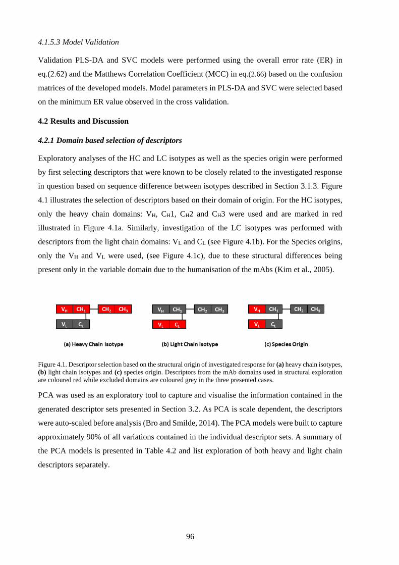
96

4.1.5.3 Model Validation

Validation PLS-DA and SVC models were performed using the overall error rate (ER) in

eq.(2.62) and the Matthews Correlation Coefficient (MCC) in eq.(2.66) based on the confusion

matrices of the developed models. Model parameters in PLS-DA and SVC were selected based

on the minimum ER value observed in the cross validation.

4.2 Results and Discussion

4.2.1 Domain based selection of descriptors

Exploratory analyses of the HC and LC isotypes as well as the species origin were performed

by first selecting descriptors that were known to be closely related to the investigated response

in question based on sequence difference between isotypes described in Section 3.1.3. Figure

4.1 illustrates the selection of descriptors based on their domain of origin. For the HC isotypes,

only the heavy chain domains: VH, CH1, CH2 and CH3 were used and are marked in red

illustrated in Figure 4.1a. Similarly, investigation of the LC isotypes was performed with

descriptors from the light chain domains: VL and CL (see Figure 4.1b). For the Species origins,

only the VH and VL were used, (see Figure 4.1c), due to these structural differences being

present only in the variable domain due to the humanisation of the mAbs (Kim et al., 2005).

Figure 4.1. Descriptor selection based on the structural origin of investigated response for (a) heavy chain isotypes,

(b) light chain isotypes and (c) species origin. Descriptors from the mAb domains used in structural exploration

are coloured red while excluded domains are coloured grey in the three presented cases.

PCA was used as an exploratory tool to capture and visualise the information contained in the

generated descriptor sets presented in Section 3.2. As PCA is scale dependent, the descriptors

were auto-scaled before analysis (Bro and Smilde, 2014). The PCA models were built to capture

approximately 90% of all variations contained in the individual descriptor sets. A summary of

the PCA models is presented in Table 4.2 and list exploration of both heavy and light chain

descriptors separately.

97

Table 4.2. PCA model summary of heavy chain (HC) descriptors and light chain descriptors (LC) according to the

four descriptor resolutions PSD1, PSD2, PSD3 and PSD4. Models were developed to capture approximately 90%

of the total variation present in the individual descriptor sets.

Chain Descriptor

Set

Number of

Descriptors

Principal

Components

Explained

Variation (%)

HC

PSD1 543 19 89.96

PSD2 817 27 90.14

PSD3 1625 68 90.02

PSD4 4367 41 90.02

LC

PSD1 272 12 90.20

PSD2 490 20 90.19

PSD3 1601 43 90.06

PSD4 2387 26 89.92

4.2.2 Exploration of HC Isotypes

In the case of the heavy chain, all samples formed three clearly defined groups when analysing

the scores from the PCA models. The PCA results of PSD1 is illustrated in Figure 4.2 where

the scores and loadings of the two first components were enough to characterise the structural

difference between the heavy chain isotypes. It can be observed that IgG1 samples are separated

from IgG2 and IgG4 samples in the first PC which explains 34.34% of the total data variation

in the descriptor set illustrated in Figure 4.2a. The second component further separates IgG2

from IgG4 samples and explained an additional 17.03% of the total data variation in the PSD1

descriptor set. The subsequent components showed no further separation of the heavy chain

isotypes but instead captured varying degrees of variation linked to the sequence variability of

the variable domain, VH (data not shown). From the loadings of the first and second PCs

illustrated in Figure 4.2b and Figure 4.2c it can be observed that the constant domains: CH1,

CH2 and CH3 contribute more significantly to the separation observed in the score plot while

the loadings of the descriptors in the variable domain VH remain close to zero. This

phenomenon is explained by investigating the VDJ gene recombination responsible for

expressing the heavy and light chain of the mAbs. All genes encoding for the full heavy chain

are located on chromosome 14 in the human genome where the VDJ region codes for the

diversity of the VH domain. Genes encoding for constant domains are located further

downstream and contain information for encoding all heavy chain isotypes (Jung and Alt, 2004,

Schroeder and Cavacini, 2010). This means the primary sequence of the VH domain cannot be

used to infer the isotype of the heavy chain due to being shared between IgG1, IgG2 and IgG4

98

and it is therefore the reason for the low contribution of the VH domain in the loadings plots

illustrated in Figure 4.2b and Figure 4.2c.

Identical observations were made for the other descriptor sets: PSD2 (see Figure C.1a and

Figure C.1b), PSD3 (see Figure C.1c and Figure C.1d) and PSD4 (see Figure C.1e and Figure

C.1f) presented in Appendix C, where the structural differences between the HC isotypes

formed distinct groups in the score plots. Some differences in explained data variation was

however observed. When using PSD1, PSD2 and PSD4, the first two PCs explained between

35-50% of the total data variation. In the PSD3 descriptor set however, PC1 and PC4 contained

the information for heavy chain isotype separation which also had a lower cumulative explained

variation of 17.08% of the total data variation. PC2 and PC3 described variation pertaining to

the sequence variability in the variable domain, VH (data not shown). The primary reason for

the lower explained variation in PSD3 compared to the other descriptor sets was due to the high

resolution where each amino acid is represented individually. This led to a higher exclusion of

descriptors from the constant domains during the data curation with more static descriptors

being removed in PSD3 compared to the descriptor sets PSD1, PSD2 and PSD4. In the latter

descriptor sets all descriptors are a sum of multiple residues and therefore contain more

variation. A summary of the PCA analysis of the four descriptor sets exploring the components

involved in the separation of the HC isotypes is presented in Table 4.3.

99

Figure 4.2. PCA exploration of VH, CH1, CH2 and CH3 descriptors from PSD1. (a) Score plot of the first two

principal components (PCs). The isotypes IgG1 are coloured red, IgG2 coloured green and IgG4 coloured blue.

(b) Loadings of the first PC. (c) Loadings of the second PC.

Table 4.3. Summary of PCA analysis listing the principal components used to observe separation of HC and LC

isotypes together with the corresponding explained data variation for each descriptor set. The last column shows

the percentage of descriptors generated from the constant domains.

Chain Descriptor

Set

Principal

Components

Explained

Variation (%)

Number of

Descriptors

Constant Domain

Descriptors (%)

HC

PSD1 1, 2 51.37 543 74.95

PSD2 1, 2 42.93 817 70.13

PSD3 1, 4 17.08 1625 45.17

PSD4 1, 2 35.57 4367 68.26

LC

PSD1 1 52.23 272 50.00

PSD2 1 54.29 490 50.20

PSD3 1 49.81 1601 47.09

PSD4 1 52.61 2387 47.47

100

4.2.3 Exploration of LC Isotypes

Similarly to the heavy chain, a very clear separation of the light chain isotypes, kappa and

lambda, was observed in the first PC for the PSD1 descriptor set seen in Figure 4.3a which

explained 52.23% of the data variation. However, contributions to the separation were not only

caused by the constant domain CL but the variable domain VL also contributed to the separation

of kappa and lambda seen in Figure 4.3b. Identical trends of PCA scores and loadings were also

observed in the other three descriptor sets: PSD2 (see Figure C.2a and Figure C.2b), PSD3 (see

Figure C.2c and Figure C.2d) and PSD4 (see Figure C.2e and Figure C.2f) presented in

Appendix C where the first principal component explained 54.29%, 49.81% and 52.61% of the

data variation, respectively. The contribution of the VH domain to the separation is due to the

fact that the VJ gene recombination of the light chain occurs at two separate chromosomes

where lambda is encoded on chromosome 2 and kappa on chromosome 22. Both chromosomes

have an individual VJ region for encoding the VL domain whose primary sequence thus

becomes dependent on the isotype that is expressed (Jung and Alt, 2004, Schroeder and

Cavacini, 2010). It therefore becomes possible to infer the light chain isotype based on the

primary sequence of the VL domain alone. This is further supported by the fact that the

explained variation of the first PC in all descriptor sets is larger than the percentage of

descriptors originating from the constant domain CL as presented in Table 4.3.

Figure 4.3. PCA analysis of VL and CL descriptors from the PSD1 descriptor set. (a) Score plot of the first two

principal components (PCs). The isotype kappa is coloured red and lambda is coloured green. (b) Loadings of the

first PC.

4.2.4 Exploration of species origin

Compared to previous observations on HC and LC isotype analysis, the PCA analysis of the

VH and VL domain descriptors did not yield a clear separation between chimeric, human and

humanised samples as can be observed for the PSD1 descriptor set in Figure 4.4a. Instead,

101

structural features related to the LC isotypes had a big influence on the captured data variation

and this was a driving force in the separation of samples as can be observed in Figure 4.4b for

descriptor set PSD1. Similar observations were made for the three other descriptors sets and are

presented in Appendix C for PSD2 (see Figure C.3a and Figure C.3b), PSD3 (see Figure C.3c

and Figure C.3d) and PSD4 (see Figure C.3e and Figure C.3f). This was not unexpected

however due to the contribution of the VL domain descriptors observed in Figure 4.3b and that

the expression of kappa and lambda light chain occurs at different Chromosomes. Another

impacting factor is the high diversity of the CDR regions in the variable domains which are the

main source of data variation in the four descriptor sets and therefore makes it difficult to

observe any species origin related separation with PCA. Even when exploring principal

components of higher order, no defined separation of the species origins can be observed in the

descriptor sets. Therefore, PLS-DA was used for classification in order to explore the extent of

data variation related to the species origins. SVC was also applied as an additional classification

method to evaluate the effect of the descriptor sets on model performance and accuracy between

methods.

Figure 4.4. PCA scores of the first and second principal components (PCs) from VH and VL domain descriptors of

PSD1. (a) chimeric (red), human (green) and humanised (blue) samples. (b) I LC isotypes kappa (red) and lambda

(green)

4.2.5 Species origin classification

To evaluate developed supervised models, the sample set was split into a calibration and test

sets with an 80/20 ratio using the CADEX algorithm in order to retain the majority of samples

and data variation for training. Using the CADEX algorithm also assured that samples in the

test set would be structurally similar to the samples in in the calibration set with regards to the

descriptor space. Table 4.4 lists the splits of the four descriptor sets with regards to the species

origins. It can be observed that the ratio of test set samples was retained at around 0.2 for the

102

three individual species origins in the four descriptor sets thus retaining representation in the

test set.

Table 4.4. Sample split with CADEX of the descriptor sets: PSD1, PSD2, PSD3 and PSD4. The number of samples

belonging to each individual species origin is listed for both the calibration and test sets.

Descriptor Set Number of

Descriptors Species Origin Calibration Test Set

Sample

Ratio (Test)

PSD1 272

chimeric 28 7 0.20

human 95 27 0.22

humanised 95 21 0.18

PSD2 488

chimeric 26 9 0.26

human 98 24 0.21


PSD3 1738

chimeric 28 7 0.20

human 92 30 0.25


PSD4 2640

chimeric 29 6 0.17

human 93 29 0.24


A summary of the performance of the developed PLS-DA and SVC models is shown in Table

4.5 for each of the four descriptor sets. In general, models developed with SVC showed a little

higher performance compared to PLS-DA in both the cross-validation and test set, thus

indicating slightly better generalisation which was most pronounced in the PSD1 and PSD2

descriptor sets. A potential reason for this may be due to the fact that all samples impact on the

on the regression prediction in PLS-DA model and therefore it is more likely to be influenced

by noisy samples. On the other hand, SVC models are developed only on an optimal subset of

the samples (support vectors) used for defining the decision boundary which thereby reduces

the influence of noisy samples on the model performance. Notwithstanding this, all models had

excellent performance in the external test set with MCC values well above 0.7 except for the

PLS-DA model developed using PSD1. Due to the differences in sample sizes between

chimeric, human and humanised samples, the MCC metric is preferred as it gives fair

representation of all classes regardless of samples size (Jurman et al., 2012). The high MCC

values are therefore an indication of strong correlation between the structural descriptors of the

VH and VL domains and the species origin. As no descriptor reduction or selection has been

performed on the descriptor sets prior to model development, a strong correlation between the

primary sequence and the species origin can be assumed.

103

In addition, the developed PLS-DA models also give an indication of the extent of the data

variation in the VH and VL domain descriptors that are correlated to the species origin. From

Table 4.5 it can be observed that roughly a quarter of the total data variation in PSD2, PSD3

and PSD4 is used for class prediction by the models whereas the variation used inPSD1 is

slightly higher with 35.93%. Thus, an estimation of the structural variation from the VH and VL

domains correlated to species origin can be inferred based on the used data variation by the

developed PLS-DA models.

Table 4.5. Summary of model performance of PLS-DA and SVC developed on the descriptor sets: PSD1, PSD2,

PSD3 and PSD4. Performance metrics for calibration (Cal), cross-validation (CV) and the external test (Test) set

are provided.

Method Descriptor

Set

Explained 𝑿 Variation (%)

Cal CV Test

MCC ER MCC ER MCC ER

PLS-DA

PSD1 35.93 0.82 0.11 0.68 0.19 0.68 0.20

PSD2 22.21 0.77 0.14 0.62 0.23 0.79 0.13

PSD3 28.70 0.95 0.03 0.75 0.15 0.96 0.04

PSD4 24.41 0.88 0.07 0.71 0.18 0.91 0.05

SVC

PSD1 - 0.92 0.05 0.72 0.17 0.85 0.09

PSD2 - 0.93 0.04 0.72 0.17 0.94 0.04

PSD3 - 0.99 0.01 0.74 0.15 0.94 0.04

PSD4 - 0.95 0.03 0.79 0.13 0.94 0.04

In addition, individual classification performance in relation to the chimeric, human and

humanised samples was assessed with receiver operating characteristics (ROC) curves on the

cross-validation results in order to understand the slightly lower MCC values compared to those

in the calibration and test set. More specifically, the area under the curve (AUC) was used as a

performance metric with a value of 0.5 indicating poor classification accuracy and a value of

one indicating perfect classification (Fawcett, 2006). The AUC values obtained from the cross-

validation on PLS-DA model developed using PSD3 data set are illustrated in Figure 4.5a and

the equivalent SVC model in Figure 4.5b. The black dashed line represents the AUC value of

0.5 thus indicating a reference border where no discrimination between classes are possible (see

Section 2.6.2). Clearly these were all above 0.9 thus indicating high accuracy. It can be observed

that most of the misclassification occurs in the humanised samples (blue line) whose AUC

values are lower compared to those of the chimeric and human samples. This is the cause for

the lower MCC values in the cross-validation compared to the calibration and external test set,

where the misclassification of humanised samples was lower (data not shown). This trend was

also observed in the cross-validation results of PLS-DA and SVC ROC curves for the remaining

three descriptor sets of PSD1, PSD2 and PSD4, illustrated in Figure C.4 in Appendix C. A

104

closer inspection of the resulting confusion matrices from the cross-validation of the four

descriptor sets showed that the misclassified humanized samples were classified as a mix of

chimeric and human (data not shown). Therefore, no particular preference was observed of the

misclassified samples that leaned more towards the chimeric class or the human class. A

potential reason for this could be due to the mix of chimeric CDRs and the human framework

regions which in unique instances, have a higher resemblance to that of fully chimeric or fully

human sequences.

Figure 4.5. ROC curves and AUC for chimeric (red line), human (green line) and humanised (blue line) samples

developed on prediction data from the cross-validation of PSD3 in (a) PLS-DA and (b) SVC. The black dashed

line represents the AUC value of 0.5 where no discrimination between classes can be made.

4.3 Summary

Based on the results presented in this chapter, the developed primary sequence-based

descriptors from Chapter 3 work well for identifying more apparent structural differences such

as the HC and LC isotypes through exploration techniques such as PCA. More advanced

supervised methods had to be used, however, to successfully separate and classify the species

origin of the used samples in order to reach higher accuracy. These exploration and

classification results were not unexpected based on the evident differences in the primary

sequence of the constant domains and the structural variation originating from humanisation of

mAbs presented in Section 3.1.5 (see Figure 3.2). Instead, the descriptor sets applicability to

these problems indicates that the developed descriptors reflect the underlying biological

features and thus the development of more advanced predictive models can be attempted. The

next logical step would be to try to develop models for prediction of mAb behaviour in more

complex experimental environments where the structural correlation to the response might be

more elusive.

105

The second important finding in this chapter is the characterisation of sources of structural

variation correlated to mAb isotypes and species origins that greatly impact the descriptors. The

described workflow in this chapter can therefore be used to determine sources of systematic

variation that is present in the mAb structure. Characterisation of such variation becomes vital

in model development as it can negatively impact model performance if the variation is

unrelated to the response which is explored in the next chapter.

107

Chapter 5

QSAR Model development: Primary sequence-based

descriptors

In Chapter 3, a novel workflow was presented for the generation of descriptor sets, capturing

varying sequence resolutions, were developed from the primary sequences of mAbs. In this

chapter the four primary sequence-based descriptor sets were investigated and applied in the

prediction of HIC retention times and mAb yields. These were chosen as response vectors for

model development due to being important parameters in pharmaceutical industries for the

assessment of productivity and product stability, respectively. The structural variation related

to the heavy and light chain isotypes as well as species origins present in the primary sequence-

based descriptor sets observed in Chapter 4 were further explored with regards to the chosen

responses. A benchmarking scheme for sequential improvement and comparison of the models

with regards to descriptor reduction and selection is also developed and presented in this

chapter.


5.1.1 Response Data

In this research, the quantitative process data published by Jain et al. (2017) was used to develop

predictive models (Jain et al., 2017). It is important to note that all constant domains in the

heavy chain were expressed as IgG1 for the heavy chain with allele IGHG1*01. The original

isotype of the light chain was retained in the explored samples where two alleles were used for

expressing either kappa (IGKC*01) or lambda (IGLC1*01) conformation.

The diversity of the of Jain dataset is illustrated in Figure 5.1 which shows the distribution of

Kappa and Lambda mAbs (Figure 5.1a), the distribution of human, humanized and chimeric

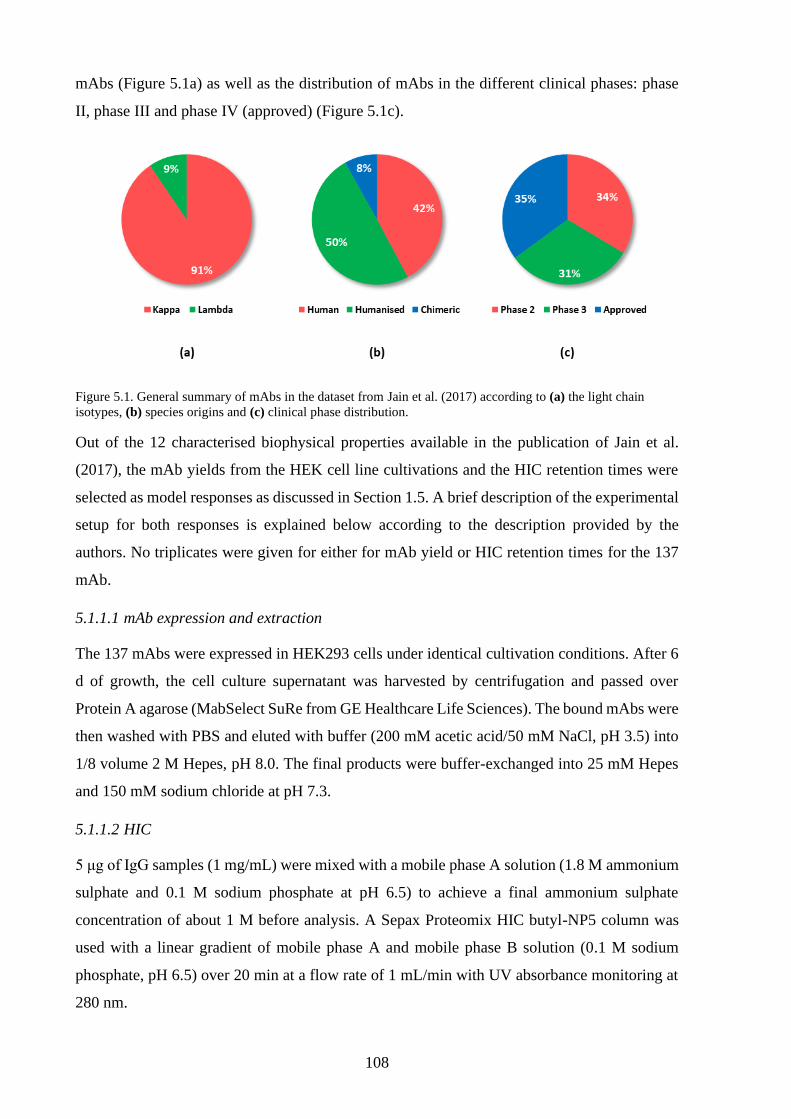
108

mAbs (Figure 5.1a) as well as the distribution of mAbs in the different clinical phases: phase

II, phase III and phase IV (approved) (Figure 5.1c).

Figure 5.1. General summary of mAbs in the dataset from Jain et al. (2017) according to (a) the light chain

isotypes, (b) species origins and (c) clinical phase distribution.

Out of the 12 characterised biophysical properties available in the publication of Jain et al.

(2017), the mAb yields from the HEK cell line cultivations and the HIC retention times were

selected as model responses as discussed in Section 1.5. A brief description of the experimental

setup for both responses is explained below according to the description provided by the

authors. No triplicates were given for either for mAb yield or HIC retention times for the 137

mAb.

5.1.1.1 mAb expression and extraction

The 137 mAbs were expressed in HEK293 cells under identical cultivation conditions. After 6

d of growth, the cell culture supernatant was harvested by centrifugation and passed over

Protein A agarose (MabSelect SuRe from GE Healthcare Life Sciences). The bound mAbs were

then washed with PBS and eluted with buffer (200 mM acetic acid/50 mM NaCl, pH 3.5) into

1/8 volume 2 M Hepes, pH 8.0. The final products were buffer-exchanged into 25 mM Hepes

and 150 mM sodium chloride at pH 7.3.

5.1.1.2 HIC

5 μg of IgG samples (1 mg/mL) were mixed with a mobile phase A solution (1.8 M ammonium

sulphate and 0.1 M sodium phosphate at pH 6.5) to achieve a final ammonium sulphate

concentration of about 1 M before analysis. A Sepax Proteomix HIC butyl-NP5 column was

used with a linear gradient of mobile phase A and mobile phase B solution (0.1 M sodium

phosphate, pH 6.5) over 20 min at a flow rate of 1 mL/min with UV absorbance monitoring at

280 nm.

109

5.1.1.3 Exclusion of samples

Out of the 137 available mAbs in the data set, 6 mAbs were excluded based on one of the

following reasons:

1) Original mAb was not of IgG class e.g. IgM

2) Original mAb was of a hybrid conformation e.g. IgG2/4

3) Experimental data for mAb was not available

This resulted in 131 mAbs being selected for further evaluation and are listed in Appendix A,

Table A.3 with corresponding experimental measurements for HIC retention times and mAb

yields.

5.1.2 Descriptor Data Generation

Structural descriptors for the 𝑿 block were generated based on the methodology presented in

Chapter 3 where four unique descriptor sets were attained: Domain based (PSD1), Substructure

based (PSD2), Single AA based (PSD3) and Running Sum based (PSD4) where PSD is short

for “Primary sequence-based descriptors”. All sequences for the variable domains VH and VL

were provided as supplementary information in the study from Jain et al (2017). Final heavy

chain sequences for descriptor generation were prepared by attaching the allele sequence

IGHG1*01 representing IgG1 isotype to the VH domains. The allele sequences IGLK1*01 and

IGLC1*01 were used and attached to VL domains of kappa and lambda isotype, respectively.


5.1.3.1 PLS

Partial Least Squares regression was performed using the NIPALS algorithm. The first 20 latent

variables were calculated to allow for a majority of the data variation in 𝑿 and 𝒀 to be captured.

A higher number of latent variables is usually not recommended as they commonly only

improve fitting of individual samples, thus causing over-fitting (Wold et al., 2001). For more

information on PLS, refer to Section 2.4.1.

5.1.3.2 SVR

Optimisation of the model parameters 𝐶 and 𝜖 was performed by using a grid search approach

on defined points over specified ranges for each parameter (for details on parameters see

Section 2.4.2). The grid points used for 𝐶 were [10-5, 10-4, 10-3, 10-2, 10-1, 100, 101, 102, 103,

104] whereas the grid points used for 𝜖 were [10-3, 10-2.5, 10-2, 10-1.5, 10-1, 10-0.5, 100, 100.5, 101].

This resulted in 90 different parameter permutations that were evaluated in the cross validation.

110



Prior to model development the data set was split into a calibration set and an external test set

to represent future samples. The Kennard-Stone (CADEX) algorithm was used to divide the

samples according to structural similarity in the form of Euclidean distance between samples

in the descriptor space (see Section 2.5.1 for more details). 80% of the samples were retained

for model calibration where the remaining 20% was kept for external testing and model

validation.

5.1.4.2 Cross-Validation scheme

A repeated k-fold cross validation scheme was applied for model development where k was

chosen to be five in order to get an 80/20 sample split ratio between training and validation

samples, respectively. 20 iterations were performed to better utilise the data set and decrease

potential impacts of outliers in the data on the cross validation. For more information, see

Section 2.5.2.


All models were validated adhering to the OECD guidelines for 𝑅2 and 𝑄2 in QSAR/QSPR

models (Veerasamy et al., 2011, Alexander et al., 2015). The guidelines state that 𝑅2 and 𝑄2

should be greater than 0.5 and 0.6 in the cross-validation and external prediction, respectively.

The thresholds for 𝑅2 and 𝑄2 in the OECD guidelines are intended to be used for early model

development to explore potential correlation of factors and descriptors related to the modelled

responses. Once characterised, additional descriptor development and adjustments can be

performed to further improve model performance. For more information on 𝑅2 and 𝑄2, refer to

Section 2.6.1.

5.1.4.4 Y-Randomisation

Y-randomisation was used to evaluate the presence of random correlation between a descriptor

set and a randomised response vector. The response vector was randomised 50 times and an

individual model was developed on each permutation. Calculated 𝑅2 and 𝑄2 values from the

50 models were then averaged. If no chance correlation is present in the descriptor set both the

averaged 𝑅2 and 𝑄2 values will be low. For more details on Y-randomisation, refer to Section

2.6.3.

111

5.1.5 Descriptor reduction and selection

The placement of the unsupervised V-WSP reduction algorithm in the model development

pipeline needed to be considered in order to generate an unbiased test set, as discussed in

Section 2.5.1. Two approaches were considered where the first scenario places the V-WSP

reduction prior to the structured data splitting using CADEX illustrated in Figure 5.2a. This

sequence however, introduces a bias due to collinearity reduction of descriptors with all

available samples in the data set. This means, that even after splitting the data set into a

calibration set (black box) and a test set (red box), the selection of the test set samples might

have been affected by the descriptor reduction of all samples. The descriptor reduction is thus

influenced by all samples and therefore becomes biased. Instead, the second scenario illustrated

in Figure 5.2b has the V-WSP reduction placed after the data splitting which ensures that only

selected calibration samples influence the descriptor reduction. This approach is thus unbiased

as it keeps the external test set samples separate throughout the model development pipeline

where descriptor reduction and selection were performed only on the calibration set. For these

reasons, development of all models in this chapter was performed adhering to the workflow

illustrated in Figure 5.2b.

112

Figure 5.2. Overview and placement consideration of the V-WSP algorithm in regards to the data splitting and the

variable selection (VS). (a) Placement of V-WSP reduction prior to structured sample splitting results in a biased

selection of descriptors due to influence from all samples. (b) Structured splitting performed before V-WSP

reduction results in an unbiased selection of descriptors due to being independent from the test set samples. Vertical

arrows represent selection of descriptors in the test set to match the calibration set.

5.1.5.1 V-WSP

The V-WSP algorithm was applied as an unsupervised reduction method to reduce the number

of descriptors in the 𝑿 block by only keeping descriptors with low correlation between them

(Ballabio et al., 2014). Procrustes goodness of fit was used as a metric to investigate how much

of the information between the original and reduced data was retained after the variable

reduction with the V-WSP algorithm (Peres-Neto and Jackson, 2001, Kendall, 1989). A

Procrustes value of zero means that the information in the data sets is identical and a value of

one means that the data sets a completely dissimilar. In the absence of any published acceptable

correlation thresholds, the thresholds for each domain were selected by empirically testing all

values from 0.5 to 0.99 with increments of 0.01. The correlation threshold was chosen based

on guidelines from Ballabio et al. (2014) where the goal of the reduction is the elimination of

redundant information and not the preservation of the data structure.

To this end, the correlation thresholds were chosen on a case by case basis for each individual

group of descriptors defined by the domains in PSD1 or the substructures in PSD2, PSD3 and

113

PSD4 therefore corresponding to inherent structural blocks in the mAbs. This was done in order

to preserve vital information present in each individual structural block of the mAb structure

and at the same time reduce the number of redundant descriptors. Reduction with V-WSP was

performed prior to any supervised variable selection method used in this research according to

Figure 5.2b.

5.1.5.2 rPLS

Supervised variable selection with rPLS was performed with PLS Toolbox 8.6.1 (Eigenvector

Research Inc) together with MATLAB 2016a (Mathworks®). An initial PLS model was

developed with selected descriptors from V-WSP reduction and the latent variable with the

smallest RMSECV was selected as a starting point for the rPLS selection. For more information

on rPLS, refer to Section 2.9.1.

5.1.5.3 GA

Supervised variable selection with Genetic Algorithm (GA) was performed using PLS Toolbox

8.6.1 (Eigenvector Research Inc) together with MATLAB 2016a (Mathworks®) and PLS as

the fitness function. A population size of 100 was used and the maximum number of generations

was set to 100. The convergence for the GA algorithm was set to 50%. Default values for the

mutation rate and the ratio of kept variables in the initial models was kept as 0.5% and 30%,

respectively. For more information on the GA algorithm, refer to Section 2.9.2.

5.1.5.4 LASSO

Supervised variable selection with L1-norm regularisation (LASSO) with SVR was applied

using the function fitrlinear in MATLAB 2016a (Mathworks®) where SVR was set as the

learner and lasso set as the regularisation method. A grid search was performed similar to that

of SVR method in Section 5.1.3.2 above in order to optimise the parameter selection. The

fitrlinear function uses 𝜆 according to eq.(5.1) instead of 𝐶 as a regularisation term as

previously described in Section 2.4.2.1.

min𝒘,𝑏,𝝃,𝝃∗

𝜆‖𝒘‖1 +1

𝑛∑(ξ𝑖 + ξ𝑖

∗)2

𝑛

𝑖=1

(5.1)

The relationship between 𝐶 and 𝜆 is described in eq.(5.2) where 𝑛 is the number of samples

(Rifkin, 2002). The relationship was used to convert the previously used 𝐶 values to that of 𝜆

instead.

114

𝐶 =1

2𝜆𝑛 (5.2)

For more details on the LASSO method, refer to Section 2.9.3.

5.1.6 Model Benchmarking

In this research, descriptor reduction and selection were performed and evaluated in subsequent

steps (Figure 5.3) in order to better investigate their impact on the model performance. For each

descriptor set, the CADEX algorithm was applied to split the available samples into a

calibration set for training (80%) and a test set for model validation (20%). Following the

outline in Figure 5.3, an initial model was developed with all descriptors in the descriptor set

of interest. A second model was then developed after V-WSP reduction had been performed on

the descriptor set. A final model was then developed after variable selection with either rPLS,

LASSO or GA had been performed on the V-WSP reduced descriptor set. The performance

metrics of 𝑅2 and 𝑄2 of the cross-validation and the test set from each of the three model were

then compared to evaluate the effect of the descriptor reduction and selection methods. This

process was repeated for each of the four descriptor sets: PSD1, PSD2, PSD3 and PSD4 when

using either PLS or SVR as modelling method.

In total, 32 models were developed in order to compare the performance of different

permutations of the presented methods. It is important to note that LASSO was only applied

when SVR was used as modelling method whereas rPLS was only applied when PLS was used

as modelling method.

115

Figure 5.3. Sequential model development and evaluation for investigation of changes in performance with

descriptor reduction and selection methods. Three models are developed on 1) all available descriptors, 2) the V-

WSP reduced descriptor set and 3) the descriptor set after supervised variable selection (VS).

5.1.7 Statistical testing

In Chapter 4, strong correlations were observed between the individual chains and their

corresponding isotypes based on exploratory analysis with PCA (see Section 4.2.2 for the heavy

chain and Section 4.2.3 for the light chain). A strong correlation was also observed between the

variable domains and the species origin when explored with PLS-DA and SVC (see Section

4.2.5). Statistical models were therefore used to establish if any significant differences were

present between groups (statistical factors) of responses. In this research the factors were

defined as the heavy chain, the light chain and the species origin of the mAbs. The heavy chain

factor consisted of three levels being: IgG1, IgG2 or IgG4. The light chain factor consisted of

two levels being: kappa or lambda. Finally, the species factor consisted of three levels being:

chimeric, human or humanised. Figure 5.4 illustrates a decision tree for choosing an appropriate

test depending on the normality and the available number of levels in the investigated factor.

Normality was tested using the Anderson-Darling test with a significance level of 0.05

(Anderson and Darling, 1952). H0 is the hypothesis that the data is normally distributed whereas

H1 is the alternative hypothesis that the data follows another distribution.

116

Figure 5.4. Decision tree for statistical testing of response data based on normality and number of available levels

for the investigated factor.

5.1.7.1 Parametric methods

Two different parametric tests were used for data that conformed to a normal distribution where

the number of available levels in the factor of interest determined which test to use. If two levels

were available, a 2-sample t-test was used to test for any significant differences between the

group means whereas if three levels were available, a 1-way Analysis of Variance (ANOVA)

was used (Krzywinski and Altman, 2014a).

5.1.7.2 Non-parametric methods

Non-parametric tests were used if the data did not conform to a normal distribution. Similar to

the parametric methods, the number of available levels in the factor of interest determined

which statistical test would be performed. A Mann-Whitney rank test was performed for factors

with two levels and a Kruskal-Wallis test was performed for factors with three levels

(Krzywinski and Altman, 2014b).

5.1.7.3 Multiple comparison

Two statistical tests were performed for each individual response, one for testing the significant

difference between the heavy chain isotypes and the other to test the significant differences

between the light chain isotypes. However, performing multiple inferences on the same data set

can cause Type I error (incorrectly rejecting H0). This is due to that fact that when the number

of statistical tests increases, the probability of any one of them being significant increases. To

adjust for this, the Bonferroni correction was used to modify the significance level according

to eq.(5.3) which gives the effective significance level for which each test needs to be tested

against (Sedgwick, 2014).

𝛼(𝑝𝑒𝑟 𝑐𝑜𝑚𝑝𝑎𝑟𝑖𝑠𝑜𝑛) =𝛼

𝑚 (5.3)

117

where 𝛼 is the desired significance level, 𝑚 is the number of performed tests and

𝛼(𝑝𝑒𝑟 𝑐𝑜𝑚𝑝𝑎𝑟𝑖𝑠𝑜𝑛) is the effective significance level.

5.2 Results and discussion

5.2.1 Selection of samples for model development

From Chapter 4 it was observed that much of the data variation in the descriptors had a strong

relationship to the heavy chain and light chain isotypes according to the PCA score plots

illustrated in Figure 4.2 and Figure 4.3, respectively. This variation is systematic and originates

from the unique structure and amino acid composition found in the individual mAb isotypes

illustrated in Figure 3.2 in Chapter 3. This is of importance as systematic variation in the 𝑿

block that is unrelated to the responses can have a negative impact on the developed models

and cause large prediction errors (Wold et al., 1998, Trygg and Wold, 2002). Therefore, prior

to model development a statistical analysis was performed to test if a significant difference was

present between response measurements related to different isotypes of the heavy and light

chain. Due to the lack of samples in the IgG2-lambda and IgG4-lambda permutations (two

samples in each group), two-factor hypothesis testing methods such as the parametric two-way

ANOVA (Fisher, 1992) or its non-parametric equivalent, the Schreier-Ray-Hare test (Sokal and

Rohlf, 1969) could not be reliably used. The unequal samples sizes can lead to a decrease in

statistical power, meaning that it becomes increasingly difficult to correctly reject H0 and thus

causing a Type II error (Rusticus and Lovato, 2014). Instead, multiple comparisons of single

factors (heavy or light chain) were performed in order to increase the sample sizes in each factor

level. Appropriate statistical tests were chosen according to the decision tree illustrated in

Figure 5.4.

Normality testing was performed for all mAb isotypes groups (kappa, lambda, IgG1, IgG2 and

IgG4) for both the HIC retention times and the mAb yields with the results presented in Table

5.1. For the HIC retention times data, normality could not be assumed for the IgG1 and IgG2

isotypes in the heavy chain as well as the kappa isotype in the light chain due to 𝑝 < 0.05.

Due to the lack of normality, non-parametric statistical methods were applied were a Kruskal-

Wallis test and a Mann-Whitney test were used for significance testing of the heavy chain

isotypes and the light chain isotypes, respectively. For the mAb yield data, normality could be

assumed in all isotypes and thus parametric statistical methods were applied in these instances.

A one-way ANOVA and a two-Sample t-test were used for significance testing of the heavy

chain isotypes and the light chain isotypes, respectively.

118

Table 5.1. Hypothesis testing of heavy and light chain isotypes using Anderson-Darling Normality Test with a

significance level of 0.05. H0 is the hypothesis that the data follows a normal distribution.

Factor

(Chain)

Level

(Isotype) Samples

HIC Yield

p Decision p Decision

LC kappa 119 0.0005 Reject H0

0.4310 Keep H0

lambda 12 0.1498 Keep H0 0.0648 Keep H0

HC

IgG1 89 0.0005 Reject H0 0.1709 Keep H0

IgG2 20 0.0097 Reject H0 0.8839 Keep H0

IgG4 22 0.1990 Keep H0 0.9414 Keep H0

Results of the statistical tests are presented in Table 5.2. The effective significance level for

each test was set to 0.025 according to the Bonferroni correction due to two multiple

comparison being performed for each response. The analysis showed that the isotype had no

significant impact on the measured responses for either the HIC retention times or the mAb

yields. Due to these findings only IgG1-kappa samples were kept for model development due

to being the most numerous in the present data set. In addition, this is also the predominantly

preferred conformation of new mAbs in clinical trials according to the IMGT database search

in Chapter 3. This resulted in 81 samples being selected from the 131 samples in the original

data set.

Table 5.2. Hypothesis testing of with a significance level of 0.025 according to the Bonferroni correction for

multiple comparisons. H0 is the hypothesis that there is no significant difference between means of different

isotypes. Non-parametric tests are referred to as NP and parametric test as P.

Response Factor

(Chain)

Levels

(Isotypes) Type Test

Equal

Variance p Decision

HIC HC 3 NP Kruskal-Wallis - 0.1201 Keep H0

LC 2 NP Mann-Whitney - 0.0721 Keep H0

Yield HC 3 P 1-Way ANOVA Yes (p=0.2270) 0.8532 Keep H0

LC 2 P 2-Sample T-test Yes (p=0.8052) 0.6326 Keep H0

It is important to remember that the heavy chain constant domains in all mAbs in the study of

Jain et al (2017) were expressed as IgG1, which introduces a bias in the statistical testing of the

heavy chain isotypes. As for the light chain, as the original isotypes were kept mostly intact

through expression with one allele for kappa and another for lambda, the impact of the light

chain isotypes on the measurements becomes more representative. As the statistical testing

above was performed through the partitioning of mAbs according to their original isotype, the

lack of significance might not hold true if identical experiments were to be performed with

unaltered mAbs. The selection of IgG1-kappa mAb samples in this case therefore ensures that

119

the measurements are more representative in terms of the original mAb structures due to less

sequence alteration.

In retrospect, even though the alteration of the original mAbs introduced a bias in the statistical

testing of the heavy chain, it gives an alternative approach for investigation of potential

variation when combined with exploratory analysis methods such as PCA, PLS-DA or SVC.

This to better control the introduction of potential systematic variation in the 𝑿 block prior to

use in model development in order to improve the prediction accuracy of the resulting models.

This becomes more relevant in environments such as industrial or clinical settings where the

original mAb structures are kept intact in order to infer information.

5.2.2 Impact of species origin

Multiple models were developed on the retained 81 IgG1-kappa samples according to the

benchmarking scheme presented in Section 5.1.6 which resulted in unique 32 models. The

model performance of each individual model is presented in Table C.4a and Table C.5a in

Appendix C for the HIC retention times and mAb yields, respectively. As can be observed,

models developed from the full descriptor set or the V-WSP reduced descriptor sets resulted in

a poor fit in terms of the cross validation 𝑅2 (0.04 – 0.22) and 𝑄2 (-0.06 – 0.15) suggesting that

the models were unable to capture the underlying correlation within the data. Adequate

improvements were first seen after a variable selection step had been performed with the GA

selection proving to be superior compared to that of rPLS and L1-SVR variable selection in

both PLS and SVR generated models. A concern, however, is the poor 𝑅2 and 𝑄2 values of the

external test set, which never reached satisfactory levels for models with adequate cross

validation metrics. All developed models therefore failed the OECD criteria of having a 𝑅2 and

𝑄2 > 0.5 in the cross validation as well as a 𝑅2 and 𝑄2 > 0.6 in the external test set.

5.2.2.1 Behaviour of species origins in PLS models

PLS was used as a diagnostic tool to further investigate the cause of the poor validation in the

test set. It was observed that initial of models for HIC retention time prediction developed on

the V-WSP reduced descriptor sets only had one component. From the error plots generated by

PLS, it was observed that the lowest RMSE value was attained with one component which

otherwise increased with higher model complexity for PSD1 (Figure 5.5a), PSD2 (Figure 5.5b),

PSD3 (Figure 5.5c) and PSD4 (Figure 5.5d). The same trends in the error was also observed

for PLS models developed for prediction of mAb yields and is presented in Figure C.5 in

Appendix C.

120

Figure 5.5. PLS error for prediction of HIC retention times in the calibration (blue line) and the cross-validation

(red line) with regards to the number of latent variables developed from the V-WSP reduced descriptor sets of (a)

PSD1, (b) PSD2, (c) PSD3 and (d) PSD4.

Further investigation was performed where a PLS models with two components were developed

for each descriptor set in order to closer investigate the samples residuals and scores. This

showed that the residuals and PLS scores were greatly affected by the species origin of the

mAbs which is illustrated in Figure 5.6 for the HIC retention times. Models used in the Figure

5.6 were developed after V-WSP reduction had been performed and they show the impact of

the species origin for the individual descriptor sets. From the influence plots for PSD1 (Figure

5.6a), PSD2 (Figure 5.6c), PSD3 (Figure 5.6e) and PSD4 (Figure 5.6g) it can be observed that

the chimeric samples tend to have higher residual values compared to humanised and human

samples. This becomes increasingly apparent with higher primary sequence resolution

illustrated in PSD2 (Figure 5.6c), PSD3 (Figure 5.6e) and PSD4 (Figure 5.6g) where the

chimeric samples are further removed from the humanised and human samples compared to

PSD1 (Figure 5.6a). As discussed in Section 3.1.5, this variation originates from the species

origin that was used to design the mAbs where mAbs originating from mouse will differ slightly

in amino acid composition compared to human mAbs in the framework regions of the variable

domains. The retained data variation from the descriptor sets used in the trained PLS models is

also affected by the systematic variation caused by the different species origins. This is

121

illustrated as score plots for PSD1 (Figure 5.6b), PSD2 (Figure 5.6d), PSD3 (Figure 5.6f) and

PSD4 (Figure 5.6h). The same trends in the residuals and PLS scores were also observed for

PLS models developed for the prediction of the mAb yield measurements where the chimeric

samples separated from the human and humanised samples which is presented in Figure C.6 in

Appendix C.

The PLS scores (𝑻) were used in this analysis as they provide better insight into the rotation of

the Latent variables e.g. what is captured by the model with respect to the PLS loadings (𝑾∗)

in the descriptor space according to the relationship 𝑻 = 𝑿𝑾∗ (Wold et al., 2001).The PLS

algorithm tries to maximise the co-variance between 𝑿 and 𝒀 but can become confused if there

is a systematic variation in 𝑿 unrelated to 𝒀 (Trygg and Wold, 2002). A separation of chimeric

samples can be observed through groupings in the lower right quadrant which is most evident

in PSD3 and PSD4 with the highest sequence resolution. This illustrates that the PLS model

becomes influenced by the different species origins and tries to separate the samples

accordingly.

122

Figure 5.6. Impact of species on PLS models developed using the HIC retention times as the modelled response

where chimeric samples are coloured red, human samples in green and humanised in blue. PLS Influence plots for

PSD1 (a), PSD2 (c), PSD3 (e) and PSD4 (g). PLS scores (T) for the individual samples for PSD1 (b), PSD2 (d),

PSD3 (f) and PSD4 (h).

123

5.2.2.2 Significance of species origins

As the variable domains were kept unaltered in the study of Jain et al (2017), additional

significance testing according to the species origins was performed to investigate potential

differences in the responses between chimeric, human and humanised samples. The study was

performed in the same way as described previously in Section 5.2.1 and is therefore only

covered briefly here. From the study, it was shown that no significant difference between the

HIC retention time means of mAbs from various species origins was observed (Table C.2 in

Appendix C) whereas a significant difference (𝑝 = 0.0093 < 0.0133) was observed between

chimeric and humanised samples for the mAb yield measurements (Table C.3 in Appendix C).

In Section 4.2.5 it was shown that classification of the chimeric, human and humanised samples

was possible with PLS-DA and SVC due to systematic structural differences in the primary

sequences of the VH and VL domains. Therefore, combined with the supporting evidence from

the diagnostic PLS models in Section 5.2.2.1 and the statistical significance testing of the

species origins, an additional sample selection was performed. For the development of models

with the HIC retentions time measurements only the humanised samples were retained (𝑁 =

45). For model development the mAb yield measurements, only chimeric and humanised

samples were retained (𝑁 = 55).

5.2.3 HIC model development on humanised samples

The cross validation and test set validation for all developed models for the HIC retention time

prediction is presented in Table C.4b in Appendix C. Models developed with PLS and SVR

using the full and V-WSP reduced descriptor sets still show a poor fit in the Cross-validation

with values around or below 0.3 and 0.2 for 𝑅2 and 𝑄2, respectively, for all descriptor sets.

Adequate Cross-validation performance was first observed after variable selection where GA

especially performed well with both PLS and SVR according to the OECD guidelines

(Veerasamy et al., 2011, Alexander et al., 2015). The SVR models developed after variable

selection with LASSO never attained good cross-validation performance in any of the data sets.

A potential cause to this might be due to that the descriptor sets contains redundant descriptors

with differing levels of collinearity toward response correlated descriptors. For the LASSO

algorithm to work properly, only a small degree of collinearity can exist between redundant and

response correlated descriptors in order for appropiate selection to be performed which is

known as the “Irrepresentable Condition” (Meinshausen and Yu, 2009).

Out of the four benchmarked descriptor sets, only the PLS and SVR models developed using

PSD1 (Domain based) and PSD4 (Running sum) passed the OECD criteria for both cross

124

validation (𝑅2 and 𝑄2 > 0.5) and external testing (𝑅2 and 𝑄2 > 0.6). Due to similar model

performance between the PLS and SVR, model selection was based on diagnostic capabilities

where the PLS models are preferred due to easier evaluation of residuals and descriptor

contribution towards 𝒀. PSD1 was selected as the preferred descriptor set due to two reasons:

1. The interpretability of descriptors in PSD1 is higher due to most of them being

physiochemical in nature. The PSD4 descriptor set in comparison consists entirely of

descriptors generated from three amino acid scales (Z-scale, T-scale and MS-WHIM).

Each descriptor represents a score generated from PCA on a set of physiochemical (Z-

scale), topological (T-scale) or electrostatic (MS-WHIM) properties and is thus a linear

combination of larger descriptor sets (see Section 3.2.2 for more details).

2. The PLS model developed on PSD1 had a lower model complexity compared to the

PLS model developed on PSD4 based on the selection of Latent variables (LVs) from

the cross validation. Three LVs were selected for the PLS model developed on PSD1

compared to 12 LVs for the PLS model developed on PSD4. This makes interpretability

of the contribution from the individual LVs more difficult in the case of PSD4 due to

the fact that deflation of 𝑿 and 𝒀 occurs each time a LV is extracted in the PLS algorithm

and models with lower complexity are preferred (Wold et al., 2001).

From the original 272 descriptors present in the full PSD1 descriptor set, 51 were retained from

the V-WSP reduction thus effectively reducing the number of descriptors by ~80%. Procrustes

index was used to evaluate the loss of information when comparing the full and V-WSP reduced

PSD1 descriptor sets. A value of 0.1434 was obtained, thus indicating that only a small portion

of the information was lost in the reduction step (Ballabio et al., 2014). This can also be

observed in Table C.4b in Appendix C for PSD1 where the of 𝑅2 and 𝑄2 values in the cross

validation and the test set remained mostly unchanged after the reduction. Out of the 51

remaining descriptors, GA selected a subset of 17 descriptors used to develop the final PLS

model. Model predictions of the calibration and test set samples are shown in Figure 5.7a as a

measured vs predicted plot. The test samples are further illustrated in Figure 5.7b as a bar plot

for easier comparison of the measured and predicted values. The model performance is

summarised in Table 5.3. The PLS regression coefficients for the selected descriptors are

illustrated in Figure 5.8.

125

Figure 5.7. HIC retention time predictions of 45 IgG1-kappa humanised mAbs with PLS model (3 LVs) developed

on the PSD1 descriptor set after reduction with V-WSP and selection with GA. (a) Measured versus predicted plot

with calibration (grey) and test (red) samples. (b) Predicted and measured HIC retention times of test set samples.

Figure 5.8. Regression coefficients of the PLS model (3 LVs) developed on the PSD1 descriptor set after reduction

with V-WSP and selection with GA.

Table 5.3. PLS model summary developed for HIC retention time prediction using the PSD1 descriptor set. Root

Mean Square Error (RMSE), R2, Q2 and model bias are listed for Calibration, Cross validation, Test set and Y-

randomisation

PLS

RMSE R2 Q2 Bias

Calibration 0.47 0.84 0.84 0.00

Cross Validation 0.67 0.63 0.62 0.01

Test 0.51 0.78 0.69 -0.27

Y-scrambled

(Average) 1.42 0.05 -0.63 0.01

Many of the test set samples were slightly over predicted which resulted in a negative bias (-

0.27). The reason for this is not known but could be a slight indication of over-fitting of the

calibration samples due to the difference in bias between the cross-validation and test set (Hastie

et al., 2009a).

126

A general trend observed in the descriptors showed that residue groups consisting mainly of

polar and charged residues such as AHR (common residues in alfa helix), NCR (negatively

charged residues) UCR (uncharged residues), PLR (polar residues), and RTR (common

residues in reverse turn/loops) had a negative contribution on the prediction, thus indicating

that mAbs with a high number of polar residues tend to have lower retention times. This is

illustrated by the negative coefficients values of the isoelectric point (Ip), charge (ECI), and

hydrophobicity (HP) where lower values in these descriptors increases the predicted retention

time. This is supported by literature where higher concentrations of salts are required to

neutralise the protein polarity in order to expose hydrophobic patches that can bind to the HIC

column (Gagnon, 1996a).

The summed molecular weight of the residues in the UCR group in the VH chain had a positive

contribution to the HIC retention time. The UCR group contains tyrosine which has the highest

weight among all the group constituents and is also the only residue with a benzene ring, thus

making it slightly hydrophobic. This indicates that with increasing number of tyrosine residues,

the HIC retention time will increase. This is supported by the descriptor describing the

theoretical number of water molecules surrounding a residue, W(U), for the UCR residues in

the VH chain where more polar residues tended to have more surrounding water molecules

compared to tyrosine. W(U) was also shown to have a strong negative correlation to the

retention time in both the VH and VL chain for polar residues further indicating a correlation

between hydrophobic residues and longer retention times, which is supported by literature

(Kennedy, 1990).

The polar area of residues (Ap) was also shown to be an important factor where larger areas

contributed to lower retention times for RTR and PLR residues due to these groups containing

mostly polar residues (see Table 3.3 in Section 3.2.1). The opposite was observed in the VL

chain where the polar area of aliphatic residues (ALR) contributed to higher retention times.

Glycine has the highest indexed polar area value in ProtDCal of all residues in the ALR group

(see Table 3.3 in Section 3.2.1) which indicates that a higher number of glycine residues in the

VL chain contributes to a higher retention time. Glycine and proline are known as unfolding

residues which indicates that a higher number of glycine residues aids in decreasing the protein

stability and thus increase binding in HIC due to exposure of the hydrophobic patches. This is

supported by literature where glycine was shown to have a negative impact on alfa helix

stability when introduced (Scott et al., 2007). This is further supported by the model where the

molecular weight (Mw) of ALR residues in the VL chain has a negative correlation to the

retention time indicating that other residues besides glycine contribute to lower retention times.

127

Also, a potential reason for the higher performance achieved with PSD1 compared to higher

resolution datasets, such as PSD2 (substructure based) and PSD3 (single amino acid based),

could be due to the introduction of more redundant descriptors in PSD2 and PSD3 which has

been shown to negatively impact model performance and descriptor selection algorithms

(Donoho, 2000, Fan and Lv, 2010). This is especially true for descriptors generated based on

the amino acid composition of the sequence where each residue in the mAb structure equally

impacts the resulting descriptors. Therefore, through generation of descriptors based on the

individual domains, a reduction of the number of redundant descriptors present in the datasets

can be achieved compared to descriptor generation for each substructure (PSD2) or each amino

acid in the sequence (PSD3).

Y-Randomisation (or Y-Scrambling) was used as a final validation step to evaluate the selection

of the descriptors (Rücker et al., 2007). A PLS model was trained on a randomised (scrambled)

HIC response vector while the sample order in the PSD1 descriptor set was kept unchanged.

This was repeated 50 times and the average of 𝑅2 and 𝑄2 for the cross validation was calculated.

A 𝑅2 value of 0.05 and a 𝑄2 value of -0.63 was obtained. This indicates that no chance

correlation is present and that the selected descriptors are important to describe the relationship

between the structure of the mAbs and HIC responses. Results are summarised in Table 5.3.

In order to appropriately evaluate if a mAb can cause potential problems in processing, a

threshold needs to be defined based on the mAb HIC retention times. In the research of Jain et

al (2017) the authors defined an upper threshold for the HIC retention time as a confidence

interval of 11.7 ± 0.6 minutes which was based on the retention times of 48 approved mAbs in

their full data set of 137 mAbs. The remaining 89 mAbs in the data set are all pending in clinical

phase II or phase III. Thus, any mAbs with a predicted HIC retention time falling above the

lower confidence limit (11.1 minutes) could be flagged due to potential risk of being

problematic in process development while mAbs falling below can be considered well-behaved.

When applying the threshold on the predictions from the PLS-GA model developed on the

PSD1 descriptor set, eight mAbs were flagged due to above the lower confidence limit:

atezolizumab, bevacizumab, certolizumab, enokizumab, obinutuzumab, otlertuzumab,

ranibizumab and tildrakizumab. Five of these mAbs have been approved while three are still in

clinical trials. However, this does not necessarily indicate that predictions falling inside or

above the threshold confidence interval will definitely fail in process development as there are

a number of factors involved that are not accounted for in this evaluation. However, historical

data in this context from approved products can be used to develop predictive models that would

128

allow for risk evaluation in early process development and thereby reduce the load on the

bioprocess pipeline.

5.2.4 mAb yield model development on humanised samples

The cross validation and test set validation for all developed models for the prediction of the

mAb yields are presented in Figure C.5b in Appendix C. The developed models behaved

similarly to the models for the prediction of the HIC retention times, where adequate

performance in the cross validation was only achieved after variable selection had been

performed. GA selection and rPLS achieved good performance for all descriptor sets while

LASSO selection suffered due to collinearity between redundant and response-correlated

descriptors explained in Section 2.9.3.

Unfortunately, no model performed well on the external test set. PLS-GA model developed

using PSD3 had a high 𝑅2 value of 0.69 but a 𝑄2 value of 0.35 in the test set thus indicating a

high offset of the predictions compared to the measured values. The difference between 𝑅2 and

𝑄2 is also greater than 0.3 thus failing the OECD criteria of |𝑅2 − 𝑄2| < 0.3 (Veerasamy et al.,

2011). PLS-GA model developed using PSD4 had similar 𝑅2 and 𝑄2 values of around 0.5 in

the test set, but this is below the desired value of 0.6 according to the OECD guidelines.

Predictions of PLS-GA model developed using PSD4 are illustrated in Figure 5.9a. It can be

observed that all calibration samples fall directly on the parity line whereas the predictions of

the test set samples have large differences between predicted and measured values as illustrated

in Figure 5.9b. This is usually an indication of the model being overfitted where the model fits

the random pattern in the noisy variables of the calibration data set (Lever et al., 2016). The

model performance is summarised in Table 5.4.

129

Figure 5.9. mAb yield predictions of 55 IgG1-kappa humanised and chimeric mAbs with PLS model (3 LVs)

developed on the PSD4 descriptor set after reduction with V-WSP and selection with GA. (a) Measured versus

predicted plot with calibration (grey) and test (red) samples. (b) Prediction and measured HIC retention times of

test set samples.

Table 5.4. PLS-GA model summary developed for mAb yield prediction using the PSD4 descriptor set. Root Mean

Square Error (RMSE), R2, Q2 and model bias are listed for Calibration, Cross validation and Test set.

PLS

RMSE R2 Q2 Bias

Calibration 1.51 1.00 1.00 0.00

Cross Validation 15.58 0.95 0.94 -0.68

Test 47.56 0.51 0.50 1.90

Several factors might impact the model development. All mAbs were expressed recombinantly

using mammalian expression vectors where the heavy and light chain were expressed from

individual cassettes (Jain et al, 2017). It has been shown that excess expression of the LC chain

compared to the expression of the HC chain facilitates higher cell productivity and mAb yield

(Bayat et al., 2018, Bhoskar et al., 2013). However, due to the unique structure of the variable

domains in the mAbs, differences in folding efficiency in the endoplasmic reticulum might

prevent an excess expression of the LC chain (Braakman and Bulleid, 2011). This is especially

important in the model development which assumes that all measured yields had identical

experimental setup which probably does not hold true as the HC:LC expression ratios will be

different between mAbs. The HC:LC ratio might therefore be an important measurement

needed for the improved model performance and can be used either as an extra input in the 𝑿

block along with the structural descriptors or, used as an additional dependent variable along

with the mAb yields.

Another potential cause for the poor performance in the test set might be the lack of necessary

variation in the data. In the case of the 𝑿 block, by using the primary sequence to generate

structural descriptors, no information can be gained regarding higher order structural

130

information such as secondary or tertiary structure and potential intra-protein interactions. More

samples might also be needed to better represent the range of 𝒀 responses, but also to introduce

more structural variation in the 𝑿 block. Noise and descriptor collinearity are also influencing

factors in the model development where the descriptor selection methods can suffer and the

wrong descriptors are thus selected (Fan and Lv, 2010).

5.3 Summary

The regulatory and quality assurance requirements for the process development of therapeutic

mAbs are becoming more stringent to ensure high product specificity and clinical safety. This

has in turn led to an increase in the number of experiments needed to characterise the design

space of a process in order to investigate the impact of process parameters on the product

quality. Today, platform approaches are becoming increasingly popular for process

development of therapeutic mAbs which limits the number of operational units that needs to be

characterised (Shukla et al., 2017). However, even with platform approaches the number of

experiments needed for process characterisation is still cumbersome and costly. This is

especially true in early process development where uncertainty is high with regards to the

manufacturability of the mAb and where the effective processing routes might not be clear.

Over recent years, the QSAR framework for in silico model development has become

increasingly popular for end point predictions of aggregation (Obrezanova et al., 2015) as well

as downstream applications (Robinson et al., 2017, Woo et al., 2015a). This makes the QSAR

framework a potentially valuable tool that can aid risk assessment in early process development

to better direct experimental designs and thus reduce costs (Karlberg et al., 2018). The use of

in silico approaches allows for more informed estimates of the potential behaviour of an mAb

in different unit operations of the process. This becomes possible by efficiently making use of

historic process data from previously established mAb manufacturing processes and therefore

constructing an expert system.

In this Chapter the importance of exploring systematic variations as a source of noise in QSAR

model development has been shown and should be considered as a critical step in the model

development. A combination of PLS and statistical testing of the responses was performed to

decrease the impact of systematic variation originating from the chain isotypes and species

origin. This had a beneficial effect on the model performance in both the cross validation and

external test set prediction after sample reduction with regards to the species origin. However,

due to the alteration of the constant domains in the original mAb structures, no conclusive

results could be drawn regarding the impact of systematic variation related to the heavy chain

isotypes IgG2 and IgG4 and the light chain isotype lambda. The workflow presented in this

131

Chapter, however, provides a structured approach for selecting samples and reducing

systematic variation that could negatively impact the model performance. In the work of

Andersen and Bro (2010), the authors stated that removal of outliers is a vital step prior to

variable selection due to the high sensitivity these methods have towards outliers. Thus, the

removal of samples with systematic variation uncorrelated to the response greatly aids variable

selection and reduces the risk of potential selection of uncorrelated variables.

Further, an efficient benchmarking scheme is presented here to validate several modelling

methods, descriptor sets and incremental descriptor reduction and selection. A model was

successfully developed for predicting HIC retention times and conformed to the model

validation scheme presented in the OECD guidelines for cross-validation (𝑅2 and 𝑄2 > 0.5)

and the test set (𝑅2 and 𝑄2 > 0.5). Though not all variation has been explained by the model,

the presented workflow is intended as an early model development step to evaluate useful

descriptors and factors affecting model performance. Additional descriptor generation and

modification might therefore help in improving model accuracy further. Based on the defined

confidence interval of 11.7 ± 0.6 from Jain et al (2017), sample predictions can easier be

assessed as potentially problematic if the prediction falls above the lower confidence limit (11.1

minutes). This however does not indicate that they are certain to fail but that caution should be

exercised and further studies are needed to characterise potential problems.

Unfortunately, no satisfactory model could be developed for the prediction of mAb yields as

indicated by the signs of overfitting evidenced by the poor test set results. A potential cause

could be the simplicity of the descriptor generation based on the primary sequence which does

not take into account higher ordered structure and stability. This is investigated further in

Chapter 7, where 3D structure descriptors will be evaluated in model development.

133

Chapter 6

3D Structure Descriptors

In this chapter descriptor generation with regards to the protein structure and dynamics is

assessed as an alternative to the primary sequence descriptors generated in Chapter 3. An

overview of protein structure model development is presented and key aspects such as the

linkage of cysteines to form disulphide bridges and structure evaluation are assessed. The

generated protein structures were used as inputs to molecular dynamics simulations in order to

relax the protein structure as well as to capture conformational dynamics of the mAbs. The

theory and implementation of molecular dynamics has been assessed in detail in order to create

a wide knowledge base to produce more realistic simulations of the mAb structures that were

used in this research but as well for future applications. In addition, strategies for modification

of protein charges with regards to the pH as well as addition of co-solvents to the simulation

system has been proposed.

The methodology for generating 3D structure descriptors follows the same approach as in

Section 3.3 in order to generate descriptor set of different resolutions. Three resolutions were

generated for the 3D structure descriptors based on the full chains, the individual domains and

the substructures. ProtDCal was implemented to generate the 3D structure descriptors but were

modified with the solvent accessible surface area of the superficial residues in order to represent

the surface properties of the mAbs.

6.1 Structure Generation

In order to generate meaningful descriptors for model development, structures need to be

available. Usually structure determination of proteins is performed by using either X-ray

crystallography or Nuclear Magnetic Resonance (NMR) which both can give a very high

atomistic resolution of the structure. Another method called Cryogenic-Electron Microscopy

(Cryo-EM) has been making its impact within this area as well due to the many improvements

134

that has been made over the years to the method and the analytical software to refine the

atomistic resolution (Carroni and Saibil, 2016, Merk et al., 2016). These methods are however

very time consuming and expensive due to the specific requirements of the methods and are not

always guaranteed to succeed (Krishnan and Rupp, 2012). Instead, the use of in silico methods

provides an alternative to estimate the protein structure and has therefore become popular in

structure determination.

6.1.1 Background on in silico methods

In silico structure prediction can roughly be divided into two schools:

1. Ab initio methods where the secondary and tertiary structure is predicted directly from

the primary sequence

2. Comparative or homology modelling where templates of existing structures are used to

predict the structure of proteins of interest.

Due to the high complexity in protein folding, pure ab initio methods do exist today but have

low accuracy and are limited to smaller proteins (< 120 residues). Extremely high

computational resources are also required in order to predict the protein folding with ab initio

methods (Lee et al., 2017). More recently, a new method based on deep learning called

AlphaFold has shown promising results and predicts likely distances between residues as well

as potential angles between chemical bonds (Evans et al., 2018).

Instead, homology modelling has been shown to offer good prediction accuracy when protein

templates exist and can be used. The high structural accuracy in homology modelling is based

on the principle that high primary sequences similarity results in high tertiary structure

similarity (Venclovas, 2011).

6.2 Homology Modelling

The approach for predicting structures in homology modelling can be broken down into five

individual steps (Marti-Renom et al., 2000):

1. Identification of evolutionary related proteins to a target protein that can be used as

templates (also known as homologs).

2. Alignment of the target protein sequence to the template.

3. Model building of target protein structure based on available structural information in

the template.

4. Error estimation of target model structure.

5. Scoring of models for comparison

135

Step one and two can usually be done in parallel where many different techniques exist to find

templates. Depending on the sequence identity that can be achieved between the target protein

and template however, alternative approaches need to be considered. When the sequence

identity is greater than 40% which is also known as the daylight zone (Rost, 1999), the search

and selection of templates can be performed using pairwise sequence alignment tools such as

Basic Local Alignment Search Tool (BLAST) (Johnson et al., 2008) or FASTA (Pearson, 1998)

from the National Centre for Biotechnology Information (NCBI). At lower sequence identity

(25-40%, also known as the twilight zone), methods such as position-specific iterated BLAST

(PSI-BLAST) (Altschul et al., 1997) or Hidden Markov Models (HMMs) (Eddy, 1998) can be

used instead for more sensitive searches to find homologs.

Different approaches exist to build the target model from the templates in step three. Commonly

used approaches are modelling by assembly of rigid bodies (Sutcliffe et al., 1987), modelling

by segment matching or coordinate reconstruction (Levitt, 1992) and modelling by satisfaction

of spatial restraints (Sali, 1995).

An initial error estimation of the produced model can usually be carried out by inspecting the

differences between the target protein sequence and that of the template. It is commonly known

that when the similarities in the alignment between the template and the target protein decrease,

the errors in the model will increase in turn. These errors originate from five sources (Fiser,

2010) related to:

1. Side-chain packing

2. Structural prediction of regions in the target protein that has shifted but otherwise

correctly aligned with the template structure

3. Structural prediction of regions in the target protein that does not have an alignment

4. Structural prediction of regions in the target protein that are misaligned in the template

structure

5. Structural prediction of target protein with wrong templates

As mentioned, the error is highly dependent on the sequence identity of the target protein and

the template. If the sequence similarity is greater than 40%, approximately 75-90% of the

predicted model structure will overlap, with an offset error of the peptide chain atoms of roughly

1 Å from their true positions. If sequence similarity goes lies in between 30-40%, the structure

overlap decreases in turn and drops to 50-75% with an offset of 3 Å in the peptide chain atoms

(Sanchez and Sali, 1998). This therefore shows the importance of appropriate selection of good

templates to be used in homology modelling. It has also been shown that the model accuracy

136

increases by using multiple templates to estimate the target protein structure (Fernandez-

Fuentes et al., 2007).

Table 6.1 lists some of the most commonly used software for model generation for mAbs. This

list is by no means exhaustive of all the different web services and stand-alone software used

for homology modelling.

Table 6.1. Commonly used homology modelling software for structure prediction of mAbs.

Software Description Reference

Web Antibody Modelling

(WAM)

Canonical modelling of CDR loops L1-3 and H1-

2 and template search for H3. CDRs are grafted

onto template frameworks

(Whitelegg and Rees,

2000)

Prediction of ImmunoGlobulin

Structure (PIGS)

Canonical modelling of all CDR loops and

grafted onto template frameworks.

(Marcatili et al.,

2014)

Rosetta Antibody Grafts selected CDR templates onto template

framework regions and energy optimises all

residues in model. Further refinement of resulting

model is performed using Monte Carlo

minimisation.

(Sircar et al., 2009)

Molecular Operating

Environment (MOE)

Antibody Modeller

Grafts selected CDR templates onto framework

templates. Energy minimisation with AMBER99

forcefields is performed to relax structure and

resolve steric clashes in grafted regions.

(Almagro et al.,

2011)

Modeller One or more templates used to represent the full

structure. Imposes conformational and sterically

restraints in the target model according to the

templates.

(Webb and Sali,

2014)

All software packages in Table 6.1, except Modeller, are specialised model generation for mAbs

and perform a separate template search for the individual framework regions and CDRs. Both

WAM and PIGS are very similar in execution when generating a target model as both methods

use canonical structure prediction of the CDR loops. This means that the CDR loops can only

assume a limited number of conformations based on the length of the loop and on the identity

of specific residues at key positions (Chothia and Lesk, 1987). The PIGS web service is,

however, more preferable as its reference database and canonical structure definitions are

frequently updated (Marcatili et al., 2014). Compared to the canonical approaches, Rosetta

Antibody focuses on resolving steric clashes in the target model that arises from the grafting of

the CDR loops onto the framework regions as well as residue overlap caused by the use

different templates (Sivasubramanian et al., 2009). The MOE Antibody Modeller is similar to

that of Rosetta Antibody, but does not perform such an extensive refinement and focuses mostly

on the regions where the CDRs were grafted onto the framework regions.

137

Research published in Almagro et al. (2011) benchmarked four antibody structure prediction

tools where PIGS, Rosetta Antibody and MOE Antibody Modeller were included and tested on

nine Fv antibody structures (VH and VL). The authors showed that accurate predictions could be

generated for most of the structure except for the H3 loop, which was distinctly different

compared to the experimental structures. It was also shown that Rosetta Antibody produced

models with fewer steric clashes compared to PIGS and MOE Antibody Modeller.

In this research, Modeller (version 9.20) was selected to generate structures for the mAbs due

to the in-house expertise available in the School of Natural and Environmental Sciences at

Newcastle University. Modeller can also be locally installed and prediction of structures can be

performed without connecting to the web server. This is usually desirable for Contract

Manufacturing Organisations (CMOs) that deal with third party sequences and therefore face

restrictions in the use of web services. Though the use of PIGS and Rosetta Antibody may have

been preferred for better accuracy in the structures of the CDR loops, these methods were

excluded due to being web services. However, further molecular dynamics simulations were

performed of the generated structures to minimise the structure energy and resolved steric and

conformational clashes (see Section 6.4).

6.2.1 Antibody Template Selection

To simplify the structure generation, it was decided to only model the Fab regions (VH, CH1,

VL and CL domains) of the mAbs due to two reasons:

1. The mAb data sets used in this research were modified and expressed with selected

allotypes (see Section 5.1.1). The heavy chain was expressed as IgG1 with allotype

IGHG1*01 whereas in the light chain the allotypes IGKC*01 and IGLC2*01 were used,

respectively, for kappa and lambda chains (Jain et al., 2017). Thus, except for the

sequence variability originating from the CL, the main source of variability originated

from the variable domains VH and VL.

2. Structure preparation of full-length mAbs is much more complex due to consisting of

four individual chains and two glycans attached in the Fc region. Information about the

glycan profiles is also extremely limited.

The template search was performed using BLAST where homologs with high sequence identity

and existing structures in the Protein Data Bank (PDB) (Berman et al., 2000) were identified.

Individual searches of the heavy and light chain of the Fab fragments always yielded template

candidates with more than 80% sequence identity. Based on this, it was decided to select a

single template for each isotype permutation of the Fab fragments for simplicity and due to

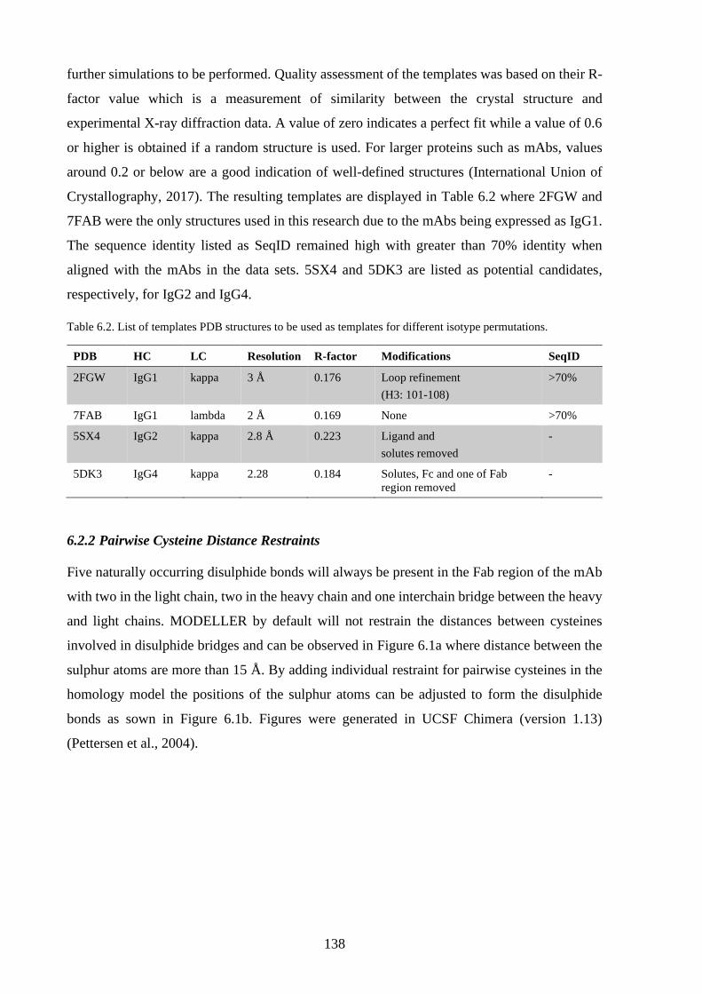
138

further simulations to be performed. Quality assessment of the templates was based on their R-

factor value which is a measurement of similarity between the crystal structure and

experimental X-ray diffraction data. A value of zero indicates a perfect fit while a value of 0.6

or higher is obtained if a random structure is used. For larger proteins such as mAbs, values

around 0.2 or below are a good indication of well-defined structures (International Union of

Crystallography, 2017). The resulting templates are displayed in Table 6.2 where 2FGW and

7FAB were the only structures used in this research due to the mAbs being expressed as IgG1.

The sequence identity listed as SeqID remained high with greater than 70% identity when

aligned with the mAbs in the data sets. 5SX4 and 5DK3 are listed as potential candidates,

respectively, for IgG2 and IgG4.

Table 6.2. List of templates PDB structures to be used as templates for different isotype permutations.

PDB HC LC Resolution R-factor Modifications SeqID

2FGW IgG1 kappa 3 Å 0.176 Loop refinement

(H3: 101-108)

>70%

7FAB IgG1 lambda 2 Å 0.169 None >70%

5SX4 IgG2 kappa 2.8 Å 0.223 Ligand and

solutes removed

-

5DK3 IgG4 kappa 2.28 0.184 Solutes, Fc and one of Fab

region removed

-

6.2.2 Pairwise Cysteine Distance Restraints

Five naturally occurring disulphide bonds will always be present in the Fab region of the mAb

with two in the light chain, two in the heavy chain and one interchain bridge between the heavy

and light chains. MODELLER by default will not restrain the distances between cysteines

involved in disulphide bridges and can be observed in Figure 6.1a where distance between the

sulphur atoms are more than 15 Å. By adding individual restraint for pairwise cysteines in the

homology model the positions of the sulphur atoms can be adjusted to form the disulphide

bonds as sown in Figure 6.1b. Figures were generated in UCSF Chimera (version 1.13)

(Pettersen et al., 2004).

139

Figure 6.1. Distance restraint of cysteines in adalimumab generated. Structure coloured as orange depicts the light

chain and structure coloured as blue depicts the heavy chain (a) Homology model without added distance restraints

to the interchain cysteines. (b) Homology model with restraint between the interchain cysteines.

6.2.3 Model Assessment

Due to the difference in the amino acid composition and the length between the template and

the mAb sequences used in this research, direct comparison with root mean square deviation

(RMSD) of atom positions is not possible. Instead initial model assessment was performed with

the inherent metric Discrete Optimised Protein Energy (DOPE) in Modeller (Shen and Sali,

2006) which is used to assess the energy of a structure or the residues in a structure. It is often

used to select a model or structure from several predictions where a lower DOPE value relates

to a more stable structure.

Figure 6.2 illustrates the normalised DOPE profiles for the template 2FGW (green line) and

adalimumab (orange line) for the heavy and light chain. As can be observed, the DOPE profiles

of the template and predicted structure overlap in most regions. The largest differences between

the template and predicted model can be observed in the regions containing the CDR loops (H1,

H2, H3 and L3) which have the highest deviation from template and thus are structurally

different. This is, however, expected due to differing amino acid compositions in the CDR

regions between adalimumab and the template. To date, accurate prediction of the CDR loops

with homology modelling is still very difficult, especially in the case of the H3 loop which has

the highest degree of varying amino acid composition and length when compared between

mAbs (Almagro et al., 2011). In comparison, the structure of the constant domains CL and CH1

overlaps in Figure 6.2a and Figure 6.2b, respectively, due to a higher sequence identity between

the template and protein target. The trends observed between the generated structure of

adalimumab and the templates were also broadly observed in all generated mAb structures in

this research.

140

Figure 6.2. DOPE score for generated model (orange line) and template (green line) for the light chain (a) and

heavy chain (b) for the aligned residues. Positions of CDR loops regions are marked by name and arrows in both

the heavy and light chain.

6.2.4 Structure considerations

It is possible to use the generated homology structures of the mAbs to generate structural

descriptors. However, four key considerations of the generated structured needed to be

addressed before doing so:

1. Origin of the templates

2. The structure is biased towards the template

3. The structure is not completely relaxed

4. Residue states in the structure might not be accurately represented

The first point involves faults or assumptions that are present in the acquired experimental

structures which might not necessarily represent reality. In the case of X-ray crystallography,

the mAbs are never naturally packed in close proximity to each other in a physiological

environment. The close proximity as a result of the crystallisation might introduce structural

artefacts in the generated 3D structures and therefore may not be completely accurate. In the

case of NMR, the structures are determined in a dynamic system where the proteins have less

self-interaction. However, the acquired 3D structures will be heavily biased towards the

environment in which the structure determination was performed e.g. pH, temperature, molality

etc.

Point two and three originate from structure generation in Modeller which estimates the target

protein structure based on the used template. Compared to specialised software, such as Rosetta

Antibody and PIGS which use unique templates for individual framework regions and CDR

141

loops in the mAbs, Modeller was used to predict the mAb structure with a single template. This

constrains the structure towards the used template and might not necessarily represent the true

structure, especially of the CDR loops. It can also cause the structure to not be in a non-relaxed

state, especially in regions where a difference in length exists between the target protein and

template. Caution thus needs to be exercised as these differences might have an impact on the

generated descriptors if the homology model if used directly for descriptor generation.

The fourth point relates to the impact of the environmental factors that can change structural

conformation and dynamics of the mAbs. In mAb manufacturing, drastic changes in the

environment are common in many operational units in the downstream process. The pH and

molality are common process factors that are changed to enhance binding and elution of mAbs

in different chromatographic columns that can drastically impact the conformation of the

protein structure.

6.3 Protein dynamics

Proteins have since long ago been described as being static structures with a specific function.

The reality however is that proteins are dynamic in nature with small structural fluctuations

over time. This is highly related to the folding energy landscape of a protein, where at a stable

conformation, many structurally similar states exist separated by small thermodynamic free

energy barriers (Bryngelson et al., 1995). Figure 6.3a illustrates a simplified example of the

energy landscape of a protein. As can be observed, fluctuations between the different states

depends heavily on the magnitude of the free energy barrier where transitions to similar state

are more frequent due to a smaller energy barrier (𝛥𝐺𝐿𝑜𝑐𝑎𝑙) whereas larger conformational

changes require more energy (𝛥𝐺𝐺𝑙𝑜𝑏𝑎𝑙). The magnitude of time is also an important factor that

needs to be considered where transition between larger conformational states takes longer due

to the cumulative kinetic energy required to overcome the large energy barriers. Figure 6.3b

illustrates changes in structural states related to the different timescale and was adapted from

the work of Henzler-Wildman and Kern (2007) as well as the work of Adcock and McCammon

(2006). It can be observed that smaller changes, such as bond vibrations and methyl rotations,

occurs at shorter timescales whereas rotation of larger solvent accessible side-chains and loop

motions lies on a timescale of nanoseconds due to larger energy differences in the barriers.

Changes in environmental factors, such as temperature, pH and molality to name a few, are also

important to consider, as they will inevitably result in a change of the energy landscape of the

protein which is illustrated as a shift from its original conformation (green line) to that new

conformation (orange line) in Figure 6.3a. This can also have an effect on the protein function

142

that is active in the original environment and inactive in the changed environment due to

conformational change.

Figure 6.3. Potential dynamics of a protein. (a) A simplified energy landscape for an arbitrary protein.

Environmental changes can drastically change the landscape as shown in the shift from the green line to the orange

line with a different conformation occupying the energy minima. (b) The time scale needed to observe local as

well as global conformational changes in a protein (adapted from Henzler-Wildman and Kern (2007) and Adcock

and McCammon (2006)).

6.3.1 Describing the system dynamics

Accurate insight into the protein dynamics can today be gained through the use of

computational simulations. The complexity of the simulations can usually be divided into four

levels of resolutions to observe a system where a short description on each has been given

below.

Quantum mechanics

The atom nuclei and electrons of a system can be described by solving the time-dependent

Schrödinger equation (TDSE) for a single particle.

Ĥ𝜓(𝒓, 𝑡) = {−

ħ2

2𝑚∇2 + 𝑉}𝜓(𝒓, 𝑡) = 𝑖ħ

𝜕𝜓(𝒓, 𝑡)

𝑑𝑡 (6.1)

𝑤ℎ𝑒𝑟𝑒 ∇2 = (

𝜕2

𝜕𝑥2+

𝜕2

𝜕𝑦2+

𝜕2

𝜕𝑧2)

143

where Ĥ is the Hamiltonian operator which corresponds to the total energy of the system, ψ the

wave function, 𝒓 the position vector of the particle (𝒓 = 𝑥𝒊 + 𝑦𝒋 + 𝑧𝒌), 𝑡 the time, ħ the reduced

Planck constant, m the mass of the particle, 𝑉 the potential energy and 𝑖 the imaginary number.

However, the TDSE is not practical for describing structure dynamics due to being

computationally intensive and it is more commonly applied for studies of faster phenomena

such a light emission absorption and emission. Instead, the time-independent form is more

commonly used to describe structure dynamics according to:

{−

ħ2

2𝑚∇2 + 𝑉}𝜓(𝒓) = 𝐸𝜓(𝒓) (6.2)

The quantum mechanics (QM) simulations provide highly detailed information about the

dynamics of the system but are also able to incorporate chemical reactions due to the

approximations of the electron orbitals. However, only smaller systems with a few atoms can

be simulated with QM due to the high complexity and computationally cumbersome

calculations (Leach, 2001d).

Classical/Molecular mechanics

Simulate the atomistic positions and movement in space by solving Newtons equations of

motion for individual particles in the system:

𝑭𝑖 = 𝑚𝑖𝒂𝑖 = 𝑚𝑖

𝑑2𝒓𝑖

𝑑𝑡2 (6.3)

where 𝑭 is the force, 𝑚 the mass of the atom, and 𝒂 the acceleration of the particle. The

atomistic interactions are approximated by using empirical force fields that describe the

potential energies of the system (see Section 6.4.1). This allows for longer simulation times up

to the scale of microseconds and even milliseconds when coarse-grained force fields are used.

A drawback with molecular mechanics (MM) is its inability to break or create covalent bonds

(Adcock and McCammon, 2006). Molecular mechanics simulations are also referred to as

Molecular Dynamics (MD).

Hybrid QM/MM

Can be used to simulate systems that are too computational expensive for standard QM but

where chemical reactions are important such as enzymatic reactions. The protein structure or

system is divided into two parts where a smaller part is simulated with QM which encloses the

144

structure responsible for the chemical reaction whereas the larger part is simulated with MM

(Liu et al., 2001).

Monte Carlo

Instead of using a deterministic system such as MD which is reliant on a time component,

Markov Chain Monte Carlo (MCMC) is a statistical approach that samples the conformation

space by randomly moving the system atoms. This means that the atom movement in a MCMC

simulation is only dependent on its immediate predecessor and therefore no temporal

relationship exists between the trials (Leach, 2001e). A drawback with MCMC is that the

simulation can become computationally expensive with increased number of atoms in the

systems due to the exponential increase in degrees of freedoms in the system if not properly

restrained.

Selection of simulation resolution

Information gained through computational molecular simulations can answer many questions

regarding the protein dynamics due to the high level of detail captured. Most commonly used

are the MD simulations which allows for longer simulation times and the ability to follow

conformational events due to being deterministic. In this research, the focus has been placed on

MD simulations due to being faster and that chemical reactions are not required for the

descriptor generation.

6.4 Molecular Dynamics

Many advancements have been made over the years to MD simulations such as theoretical

improvements with new empirical force fields as well as practical improvements of simulation

speed and increase the system size (Rauscher et al., 2015). One such advancement is the

incorporation of Graphical Processing Units (GPUs). State-of-the art graphics cards contains

thousands of cores which can be used to divide the molecular system into smaller parts which

can be run in parallel. This shifts the workload from the Central Processing Unit (CPU) to the

GPU which calculates the forces on the atoms whereas the CPU is free to allocate data and

combine the results of the smaller parts (Loukatou et al., 2014).

Improvements in simulation time can also be gained through simplification of the system with

a so-called coarse-grained approach. Instead of representing all atoms in the system (referred

to as all-atom or atomistic), a coarse-grained simulation may represent each amino acid side-

chain as a single cluster with their corresponding force fields. This drastically reduces the

degrees of freedom in the system (see Section 7.2.2.1) which in turn decreases the necessary

145

number of calculations that needs to be performed (Kmiecik et al., 2016). One of the most

commonly used coarse-grained force fields is MARTINI which has been shown to achieve

simulation results close to that of atomistic simulations (May et al., 2013). Figure 6.4 illustrates

the applicability domains of atomistic and coarse-grained models with regards to the system

size and simulation time (adapted from Kmiecik et al (2016)).

Figure 6.4. The relationship between the system size and possible simulation times for QM, atomistic and coarse-

grained simulations. Loss of information is inevitable when moving to simplified estimation of the system such as

atomistic and coarse-grained representation which are illustrated by the green and orange graphs, respectively

(adapted from Kmiecik et al. (2016)).

As shown, larger systems and longer simulation times become possible when moving from

more computationally intensive QM calculations towards system approximations with MM

calculations. With further decrease in degree of freedoms in a system resulting from the move

from an atomistic to a coarse-grained setup, the system size and simulation times can be

increased even further. However, caution needs to be exercised as a system simplification step

inevitably leads to a loss of information of protein dynamics which will no longer be captured

in the simulations. This can easily be visualised when comparing the energy landscapes of an

atomistic model to those of a coarse-grained model represented as the green and orange energy

graphs in Figure 6.4, respectively. In the atomistic model, the rotations of the side chains and

bond vibrations will more or less be intact resulting in many local conformational minima in

the energy landscape. In a coarse-grained model however, side-chains are treated as a single

cluster and therefore lack many of the local motions. The energy landscape of a coarse-grained

will therefore be smoother but will follow the general trend of an atomistic model. Therefore,

it is advised to choose the simulation resolution based on the area of investigation where an

atomistic model is recommended to capture local motions and a coarse-grained model

recommended to capture global motions.

146

A popular approach to increase the resolution is to use multiscale modelling where major events

are first captured with a coarse-grained model. Events of interest can be further modelled by

reconstructing the coarse-grained model to atomistic resolution at specified time points (Heath

et al., 2007). This allows for more detailed information about the system to be captured and

avoids the need of performing longer atomistic simulations in the beginning.

A list of commonly used MD software packages is presented in Table 6.3. For the purpose of

this research, GROMACS (version 5.1.4) was selected due to the in-house expertise available

at Newcastle University. In addition, GROMACS is able to incorporate the MARTINI force

field used for coarse-grained modelling. This is of added benefit due to the increasing popularity

of MARTINI and the many advancements made to the force field which have increased the

model accuracy to almost rival that of atomistic (Marrink and Tieleman, 2013).

Table 6.3. Non-exhaustive list of popular MD simulation software.

Software Atomistic Coarse-

Grained

GPU

support

OS Availability Reference

AMBER YES NO YES Window,

Linux

Commercial (Salomon‐Ferrer

et al., 2013)

CHARMM YES NO YES Linux Commercial (1) (Brooks et al.,

2009)

GROMACS YES YES (2) YES Linux Free (Van Der Spoel

et al., 2005)

MOE YES NO YES Windows,

Linux

Commercial (MOE, 2018)

NAMD YES YES (2) YES Windows,

Linux

Free (Phillips et al.,

2005)

(1) A reduced version of CHARMM can be acquired for free. (2) Uses the MARTINI force fields

6.4.1 Force Fields

In order to calculate the forces acting in a system, the potential energy, 𝑈(𝒓𝑁), for each atom

needs to be defined where 𝒓𝑁 = (𝒓1, 𝒓2, … , 𝒓𝑁) are the Cartesian coordinates for the N atoms

in the system. The molecular interactions can be approximated with mathematical expressions

to represent different interactions of the system. An equation for approximation of the total

potential energy in a system can be written as (Leach, 2001b):

𝑈(𝒓𝑁) = 𝑈𝑏𝑜𝑛𝑑𝑠 + 𝑈𝑎𝑛𝑔𝑙𝑒𝑠 + 𝑈𝑡𝑜𝑟𝑠𝑖𝑜𝑛𝑠 + 𝑈𝑐𝑜𝑙𝑢𝑚𝑏 + 𝑈𝑣𝑑𝑤 (6.4)

147

As shown, the interactions can be divided into two categories of bonded (green solid lines) and

non-bonded (red and black dashed lines) interactions shown in Figure 6.5a and Figure 6.5b,

respectively.

Figure 6.5. (a) The bonded interactions originating from bond stretching, angle bending and bond torsion

(rotation). (b) The non-bonded interactions originating from electrostatic and van der Waals potentials (adapted

from Allen (2004) and Leach (2001b)).

The bonded interactions represent the potential energies originating from the covalent bonds

and steric conformation of the structure in the form of bond stretching, angle bending and

torsion from bond rotations. Resulting potential energies from the bonded interactions are

shown in Figure 6.6 and were adapted from the GROMACS manual 5.1.4 (Abraham et al.,

2016).

The potential from the bond stretching between two atoms is approximated using Hooke’s law

for harmonic potentials (see Figure 6.6a) to define the potential well:

𝑈𝑏𝑜𝑛𝑑𝑠(𝑟𝑖𝑗) =

1

2𝑘𝑖𝑗

𝑏 (𝑟𝑖𝑗 − 𝑟𝑒𝑞)2 (6.5)

where 𝑟𝑖𝑗 = |𝒓𝑖𝑗| and 𝒓𝑖𝑗 = 𝒓𝑖 − 𝒓𝑗

which in turn takes on the following expression for the force:

𝑭𝑏𝑜𝑛𝑑𝑠𝑖 (𝒓𝑖𝑗) = −𝑘𝑖𝑗

𝑏 (𝑟𝑖𝑗 − 𝑟𝑒𝑞)𝒓𝑖𝑗

𝑟𝑖𝑗 (6.6)

148

The constant 𝑘𝑖𝑗𝑏 is the spring constant where a higher value prevents greater bond stretching.

The variable 𝒓𝑖𝑗 is the bond vector between two atom positions with the magnitude or bond

length 𝑟𝑖𝑗. The constant 𝑟𝑒𝑞 is usually referred to the natural bond length where the potential

energy is at its lowest.

The potential energy from angle bending (see Figure 6.6b) is also frequently described using

Hooke’s law but uses the angle between two bonds instead of the bond length:

𝑈𝑎𝑛𝑔𝑙𝑒𝑠(𝜃𝑖𝑗𝑘) =

1

2𝑘𝑖𝑗𝑘

𝜃 (𝜃𝑖𝑗𝑘 − 𝜃𝑒𝑞)2 (6.7)

The potential energy of the angle bending takes on the following expression for the force:

𝑭𝑎𝑛𝑔𝑙𝑒𝑠

𝑖 (𝜃𝑖𝑗𝑘) = −𝑑𝑈𝑎𝑛𝑔𝑙𝑒𝑠(𝜃𝑖𝑗𝑘)

𝑑𝒓𝑖

𝑭𝑎𝑛𝑔𝑙𝑒𝑠𝑘 (𝜃𝑖𝑗𝑘) = −

𝑑𝑈𝑎𝑛𝑔𝑙𝑒𝑠(𝜃𝑖𝑗𝑘)

𝑑𝒓𝑘

𝑭𝑎𝑛𝑔𝑙𝑒𝑠𝑗

(𝜃𝑖𝑗𝑘) = −𝑭𝑎𝑛𝑔𝑙𝑒𝑖 − 𝑭𝑎𝑛𝑔𝑙𝑒

𝑘

(6.8)

where 𝜃𝑖𝑗𝑘 = arccos (

𝒓𝑖𝑗 ∙ 𝒓𝑘𝑗

𝑟𝑖𝑗𝑟𝑘𝑗)

The constant 𝑘𝑖𝑗𝑘𝜃 is the spring constant where higher values prevent bending making the

structure more rigid. The variable 𝜃𝑖𝑗𝑘 is the angle between two connecting bonds from three

atomic positions. The constant 𝜃𝑒𝑞 represents the natural angle based on the atom types of the

three atoms.

The torsion potential is almost always expressed as a cosine Fourier series expansion with m =

1,2,… ,M (Leach, 2001b). The torsion is defined by three connecting bonds and therefore

involves four atomic coordinates (see Figure 6.5a) according to:

𝑈𝑡𝑜𝑟𝑠𝑖𝑜𝑛𝑠(𝜑𝑖𝑗𝑘𝑙) =

1

2∑𝑘𝑖𝑗𝑘𝑙

𝜑,𝑚(1 − cos(𝑚𝜑𝑖𝑗𝑘𝑙 − 𝛾𝑚))

𝑚

(6.9)

The expression for the resulting torsion force is not shown due to being much more extensive

than previous forces. The constant 𝑘𝑖𝑗𝑘𝑙𝛷,𝑚

is the magnitude of the torsion potential, m represents

149

the which series in the series expansion, the variable 𝜑𝑖𝑗𝑘𝑙 is the torsion angle and 𝛾𝑚 is the

phase factor which describes at which angle the potential energy is at its lowest. Figure 6.6c

shows the potential energy from the torsion of an arbitrary molecule bond where the energy is

at its lowest when with less steric clashes occurs (staggered conformation) and at its highest

when more steric clashes occurs (eclipsed conformation).

Figure 6.6. Potential energy of bonded interactions. (a) An approximation of the potential energy in the bond

stretching using Hooke’s law as a function of the distance between two bonded atoms. (b) The potential energy

from angle bending as a function of the angle between two connecting bonds and approximated with Hooke’s law.

(c) Approximation of the potential energy from bond torsion as a function of the bond angle. Highest potential is

observed in eclipsed conformation and lowest in staggered conformation (adapted from the GROMACS manual

5.1.4).

The non-bonded interactions represent the potential energies originating from electrostatic and

van der Waals interactions. These include both internal interactions in the protein as well as

external interactions from the solvate. Resulting potential energies from the non-bonded

150

interactions are shown in Figure 6.7 and were adapted from the GROMACS manual (Abraham

et al., 2016).

Potential energies originating from van der Waals interactions are commonly described by

using the Lennard-Jones (Jones, 1924) equation:

𝑈𝑣𝑑𝑤(𝑟𝑖𝑗) = 4𝜀 [(

𝜎

𝑟𝑖𝑗)

12

− (𝜎

𝑟𝑖𝑗)

6

] (6.10)

The potential energy takes on the following form for the resulting force:

𝑭𝑣𝑑𝑤

𝑖 (𝑟𝑖𝑗) = 4𝜀 [12𝜎12

𝑟𝑖𝑗13 − 6

𝜎6

𝑟𝑖𝑗7]

𝒓𝑖𝑗

𝑟𝑖𝑗 (6.11)

The constant 𝜀 defines the depth of the potential well whereas the constant 𝜎 defines the

distance between two atoms when the potential is at a minimum. It can be observed in Figure

6.7b that an arbitrary attraction occurs when the distance is 3 Å between two atoms, this is

similar to that of the Morse potential seen in Figure 6.6a but lacks a physical bond. The

magnitude of the Lennard-Jones potential is also much lower compared to that of the Morse

potential.

The electrostatic potential energy between two charged atoms in the system can be described

by using the following expression:

𝑈𝑐𝑜𝑙𝑢𝑚𝑏(𝑟𝑖𝑗) =

1

4𝜋𝜀0

𝑞𝑖𝑞𝑗

𝑟𝑖𝑗 (6.12)

The electrical potential takes on the familiar expression of coulombs law when converted into

the resulting force:

𝑭𝑐𝑜𝑙𝑢𝑚𝑏

𝑖 (𝒓𝑖𝑗) =1

4𝜋𝜀0

𝑞𝑖𝑞𝑗

𝑟𝑖𝑗2

𝒓𝑖𝑗

𝑟𝑖𝑗 (6.13)

The variable 𝑞 is the charge of the atom and 𝜀0 is known as the permittivity constant. It can be

observed through Figure 6.7b that the potential energy increases with shorter distance between

charges. When of same charge the atoms will repel each other while different charges will

attract each other.

151

Figure 6.7. Potential energy of non-bonded interactions. (a) The electric potential as a function of distance between

two charged points. (b) The van der Waals potential approximated with Lennard-Jones potential (green line) as a

function of the distance between two non-bonded atoms. Consists of one repulsion (orange dashed line) and one

attraction (orange full line) component (adapted from the GROMACS manual 5.1.4).

It should be mentioned that the hydrogen bond, which is a common non-bonded interaction in

proteins, is not treated as a separate bond type in the force fields but rather as a combination of

Lennard-Jones and electrostatic potential instead.

In comparison to the bonded interactions, the number of non-bonded interactions that needs to

be evaluated in a system increases with the order of 𝑁2 due to the fact, that any pair of atoms

in the system can interact. To avoid time-consuming simulations or, in worst cases, system

crashes, cut-off schemes are used to reduce the number of potential long-range calculations that

needs to be performed. Commonly applied is Particle Mesh Ewald (PME) summations which

consists of short-range contributions and long-range contributions. Short-range interactions are

determined by a predefined cut-off radius (commonly 1 nm) to identify neighbouring atoms to

the atom of interest. If the distance is less than the defined cut-off radius, the atom is included

in the force calculation and a so-called neighbours list is created that specifies the neighbouring

atoms to the atom of interest which was first proposed by Verlet (1968). Long-range

interactions are atoms with distances exceeding the defined cut-off radius from the atom of

interest and are instead calculated with Fourier transform from the real space to the reciprocal

space which allows for faster computation.

As can be observed, equations (7.5), (7.7), (7.9), (7.10) and (7.12) contain parameters for

optimal bond lengths, angles, potential wells, force constants etc that needs to be specified. Put

in simple terms, a force field is a list of parameter values for different atom types with

corresponding equations that are used to calculate the potential energy of the system (Allen,

152

2004). Ii is important to note that an atom type should not be confused with an element from

the periodic table. The definition of an atom type here involves the hybridisation state and/or

the charge of the atom as well as the type of connected atoms. For example, carbon will have

several atom types which describe different hybridisation states and surroundings. This in turn

means that they will behave slightly different from each other and therefore need to be described

with a unique set of parameters for each atom type. This also makes the number of atom types

listed in the force fields much more numerous than the number of elements in the periodic

system.

Table 6.4 gives a non-exhaustive list of popular force fields that are used in MD simulations

currently where several different versions of the AMBER, CHARMM and GROMOS force

fields exists. Only slight variations exist between the different force fields which include

differences in parameter values or slight differences in the potential energy equations, usually

in the non-bonded interactions (Allen, 2004). The estimation of the parameters for different

atom types are almost always carried out with QM calculations or taken from experimental

measurements (Kmiecik et al., 2016).

Table 6.4. Non-exhaustive list of popular force fields.

Force Field Parameter determination Reference

AMBER Multi-purpose force field widely used for proteins and DNA

simulations

(Cornell et al., 1995)

CHARMM Multi-purpose force field widely used for both small and

macromolecule simulations

(Brooks et al., 1983)

GROMOS First developed for simulations of protein or DNA in

hydrophobic solvent. Now the force field is multi-purpose.

(Oostenbrink et al.,

2004)

OPLS-AA Multi-purpose force field (Jorgensen et al., 1996)

In this research, the atomistic amber99sb-ILDN force field was used to simulate the dynamics

of the antibody Fab fragments. The authors Lindorff‐Larsen et al. (2010) modified the original

amber99sb force field to more accurately describe side chain torsions in a protein.

6.4.2 The MD Algorithm and Time Integration

The global MD algorithm is shown in Figure 6.8 and consists of four steps (adapted from the

GROMACS User Manual 5.1.4 (Abraham et al., 2016)).

In the initial step of any MD simulation, the positions and velocities for each atom in the system

need to be specified. Atom positions can be acquired through PDB files from either

experimental data or a predicted structure (see Section 6.2). Usually no velocities are available

when starting a new simulation project unless it is a continuation of a previous simulation. In

153

these cases, the Maxwell-Boltzmann distribution can be used to randomly assign initial

velocities to all atoms in the system at a given temperature T.

𝑝(𝑣𝑖) = √

𝑚𝑖

2𝜋𝑘𝑇exp (−

𝑚𝑖𝑣𝑖2

2𝑘𝑇) (6.14)

Lastly, a force field needs to be selected to describe the potential energy function and

interactions in the system and will not be changed throughout the simulation.

The forces in the system are then calculated from the potential energy of the system in step two.

The resulting force on each atom is calculated as a vector sum based on all interactions from

surrounding atoms (see Section 6.4.1). This step also involves all corrections applied to the

system in order to maintain or change the thermodynamic macrostate by controlling the system

volume, temperature and pressure. This is further explained in Section 6.4.4.

Figure 6.8. Four steps of the global MD algorithm. Step 1) Positions and initial velocities are assigned and a force

field chosen. Step 2) Calculation of resulting forces on all atoms in the system. Step 3) Updates the positions and

154

velocities of all atoms in the system. Step 4) Saves specified information to a log file (adapted from the

GROMACS User Manual 5.1.4).

The third step in the MD algorithm updates the positions of all atoms in the system based on

the calculated forces in step two. This is done by numerical integration in order to approximate

the resulting velocities and positions of the atoms in the system. Two popular approaches that

commonly used to perform the integration are the Verlet velocity algorithm (Swope et al., 1982)

and the Verlet leapfrog algorithm (Hockney and Eastwood, 1988) where the later will be

investigated more thoroughly. The leapfrog algorithm updates the atom position and velocity

according to:

𝒗𝑖 (𝑡 +

1

2∆𝑡) = 𝒗𝑖 (𝑡 −

1

2∆𝑡) +

𝑭𝑖(𝑡)

𝑚𝑖∆𝑡 (6.15)

𝒓𝑖(𝑡 + ∆𝑡) = 𝒓𝑖(𝑡) + 𝒗𝑖 (𝑡 +

1

2∆𝑡) ∆𝑡 (6.16)

where 𝒗𝑖 and 𝒓𝑖 are the velocity and the position of atom 𝑖 and ∆𝑡 is the timestep used in the

numerical integration. In the leapfrog algorithm, positions are updated at each full time-step

(𝑡 + ∆𝑡) (6.15) while the velocities are updated at each half time-step (𝑡 + ∆𝑡/2) (6.16) thus

making the atomic position and velocity jumping over each other like two leaping frogs. This

allows for more accurate calculations of the velocities as compared to if the positions and

velocities would have been synchronised.

In MD simulations, the time step ∆𝑡 needs to be sufficiently large in order to efficiently simulate

the protein dynamics without unnecessary resampling of the conformational space. However,

if a too big a time step is selected it can cause instability and inaccuracies when the subsequent

atom positions are calculated resulting in unfavourable conformations and high potential

energies. A rule of thumb is to adapt the time step to the smallest local motion in the system in

order to avoid this problem. Usually, a default time step of 2 fs is used in MD simulations today.

It is important to note that the vibration period of the hydrogen bonds is shorter than the timestep

of 2 fs and therefore cannot be accurately sampled. In order to avoid instability, the hydrogen

bonds are constrained with the LINCS algorithm which keeps the length of the hydrogen bond

constant throughout the simulation.

6.4.3 Periodic Boundary Conditions

Even with advancement of computational power the actual size of the system to be simulated

is extremely small compared to a real-world setting. This also means that the surface to volume

155

ratio in the simulation is much higher compared to a real experimental setup which can

introduce artefact caused by surface effects. Unless this is the aim with the simulation, a way

to avoid this problem is to use so called Periodic Boundary Conditions (PBCs). In the event

where a molecule exits the simulation box it will automatically re-enter the system on the

opposite side with its trajectory preserved as can be seen in Figure 6.9a. This effectively means

that the system has been enlarged by infinity. Caution needs to be exercised in order to avoid

self-interaction of example a protein. This is commonly avoided by making sure that the

distance between the protein to the edge of the simulation box is at least three solvation layers

wide which roughly translates to 0.9 – 1.0 nm (González, 2011). This concept is shown in

Figure 6.9b where the cut-off radius is illustrated as the dashed red circles surrounding a particle

of interest. The system size is adequately chosen in this case where the particle of interest will

not self-interact as well as overlap between the circles have been avoided thus making sure that

potential water molecules in the systems are not affected by the particle from adjacent boundary

cells (adapted from (González, 2011)).

Figure 6.9. The application of the periodic boundary condition in a simulation. (a) Movement of particles out of

the simulation box will enter the opposite. (b) Depicts the cut-off radius for long-range interactions as the dashed

red circle and the importance of choosing a proper box size in order to avoid overlap and self-interaction (adapted

from González (2011)).

The shape of the PBC can also be changed in order to optimise the simulation if a rectangular

box introduces too many water molecules into the system when solvated. Preferably, the shape

of the PBC should be chosen so it reflects the underlaying geometry of the macromolecule e.g.

a Truncated Octahedron or a Rhombic Dodecahedron can be used for simulation of globular

156

proteins whereas a hexagonal prism can be used for simulation of a rod like protein or DNA

(Leach, 2001a).

6.4.4 Thermodynamic macro and microstates

In order to properly simulate a system, it is important to make sure that the simulation accurately

captures its thermodynamic properties. So far, the main discussion has been about atom

interactions and motions in a system of interest. The positions and velocities of the atoms are

commonly referred to as thermodynamic microstate variables, which in turn define the

thermodynamic macrostate properties of volume, pressure and temperature in a system. It is

important to remember that a macrostate with a set volume, temperature and pressure can be

described by several different microstates whereas the opposite is not possible where instead

one microstate will have single corresponding macrostate. This is easier understood when

considering a smaller system containing a few atoms with defined positions and velocities. If

two of the atoms were to swap velocity directions and magnitudes, the microstate of the system

would change due to the change in the microstates variables whereas the macrostate will still

be conserved.

This is an important aspect that needs to be considered in order to correctly simulate a real-

world experiment where a specific temperature, volume and pressure are used. The absolute

temperature of a system can be calculated by using the total kinetic energy shown in (6.17)

below.

𝐸𝐾𝑖𝑛 =1

2∑𝑚𝑖𝑣𝑖

2

𝑁

𝑖=1

=𝑘𝐵𝑇

2(3𝑁 − 𝑁𝐶) (6.17)

𝑘𝐵is Boltzmann’s constant, 𝑁𝐶 is the number of constraints applied on the system and 3𝑁 − 𝑁𝐶

is the total number of degrees of freedom in the system. The pressure, 𝑝, can be calculated by

using the total kinetic energy and the virial of the system shown in (6.18) below.

𝑝 =

2

3𝑉(𝐸𝐾𝑖𝑛 − ⟨𝑇⟩) (6.18)

⟨𝑇⟩ = −

1

2∑∑⟨𝐹𝑖𝑗𝑟𝑖𝑗⟩

𝑁

𝑗>𝑖

𝑁

𝑖

(6.19)

157

𝑉 is the system volume and ⟨𝑇⟩ is the virial or the expected value of the sum of products between

atom coordinates and the forces acting on them (Berendsen et al., 1984). The brackets represent

the average value over time.

When performing a MD simulation, several different simulation ensembles are available that

that restrains the system by keeping some of the thermodynamic properties constant while

allowing other to fluctuate. The choice of which ensemble to use depends heavily on how the

system should behave and the aim of investigation. Three commonly used ensembles are NVE,

NVT and NPT where all ensembles have a constrained number of atoms (N). The NVE

ensemble is a so-called micro-canonical ensemble with constrained volume (V) and energy (E)

and is most often used to study the conformational energy landscape. The NVE ensemble

should never be used to equilibrate a system as the desired temperature can never be reached

when the energy is conserved. The NVT ensemble is a canonical ensemble and thus in thermal

equilibrium with constrained volume and temperature (T). This type of ensemble is often used

to simulate biological reactions. The NPT ensemble is an isothermal–isobaric ensemble with

constrained pressure (p) and temperature and is commonly used to simulate chemical reactions

in environments where the pressure is maintained such as open atmosphere reactions. Both the

NVT and NPT ensembles are commonly used for system equilibration to reach specified

temperature and pressure in order to replicate experimental environments. More detailed

descriptions on the different ensembles are reviewed elsewhere (Brown and Clarke, 1984).

In order to maintain the desired thermodynamic parameters of a system in a simulation, the use

of so-called coupling schemes becomes necessary in order to control parameters of interest such

as the temperature and pressure of the system.

The temperature can be controlled by using thermostats. The Berendsen (Berendsen et al., 1984)

and Velocity-rescaling thermostats (Bussi et al., 2007) controls the temperature by directly

scaling the velocities of the atoms in the system through first-order decay. The Berendsen and

Velocity-rescaling thermostats are known as coupling methods. Alternatively, the Nosé-Hoover

thermostat (Nosé, 1984, Hoover, 1985) can be used and works by adding an extra correction

term to the Newton’s equation of motion seen in Figure 6.8 which subtracts or adds to the atom

velocities in the system if the temperature is too warm or too cold, respectively. The Nosé-

Hoover thermostat is a so-called extended system dynamics method. The three listed

thermostats are virtually linked to a heat bath with constant temperature through which heat is

exchanged as illustrated in Figure 6.10. This also means that the energy will no longer be

conserved in the system and will change depending on the temperature difference between the

heat bath and the system of interest.

158

Figure 6.10. A system coupled to a virtual heating bath illustrating the heat exchange between the heat bath and

the system of interest (adapted from Ghiringhelli (2014)).

The pressure, similarly to the temperature, is controlled by using barostats. A commonly used

weak coupling method is the Berendsen barostat (Berendsen et al., 1984) which is similar to

the Berendsen thermostat but instead scales the dimensions of the system in order to achieve

the desired reference pressure. Alternatively, the Parrinello-Rahman barostat is an extended

system dynamics method similar to that of the Nosé-Hoover thermostat where the volume

becomes and extra variable (Parrinello and Rahman, 1981). This allows the system size to vary,

thus contracting or expanding the system if the pressure is too low or too high, respectively,

compared to the desired reference pressure.

6.4.5 GROMACS System Equilibration

In this research, the GROMACS guidelines for system equilibration were used prior to any

production runs in order to emulate real-world experimental conditions (Abraham, 2014). Four

equilibration steps were performed with a final production run at the end according to the steps

below:

1. Solvation of the system

2. Energy minimisation (EM)

3. Temperature increase to target value through NVT ensemble

4. Adjustment of pressure to target value through NPT ensemble

5. MD production run

The first step involves specifying the periodic boundary conditions to define the simulation box

and then filling the empty space with water molecules and counter ions to buffer the system. A

common practice is to add chloride and sodium ions to counter the charges of the protein to get

a system with a net charge of zero.

The EM is a crucial step that prevents the system from “blowing up” when equilibrated due to

potential close proximities and steric clashes between atoms which can result in large forces.

These clashes originate partly from the protein structure that, if predicted, might not be

159

completely relaxed and therefore structurally unfavourable (see Section 6.2.4). Another source

is clashes originating from the addition of the solvate to the system where potentially some

water molecules might have been placed too close to the protein. The energy minimisation

conformationally resolves these clashes by relaxing the system through rotational and

directional motions of the clashing atoms, thus lowering the energy of the system (Leach,

2001c). Several methods exist to perform the EM where derivative minimisation methods are

most commonly used. First-order methods such as steepest descent and conjugate gradient are

fast methods that use the first derivative or gradient to find the energy minima but with the

drawback that they can get stuck in local minima. Second-order derivative methods, such as

quasi-Newton and L-BFGS, include information about the energy curvature and are less likely

to get stuck at local minima but are more computationally intensive due to the need to calculate

the Hessian matrix (second derivative matrix). For more detailed information on the listed

minimisation methods, refer to the following work (Schlick, 1992). The steepest descent

minimisation was used in all simulations due to its speed compared to quasi-Newton and L-

BFGS.

In the third equilibration step, an NVT ensemble was used to raise the temperature of the system

to a desired target value. Initial velocities in the system were assigned with the Maxwell-

Boltzmann distribution presented in eq.(6.14) according to a target temperature of 300 ºK.

Position restraints were added to the backbone of the proteins in order to avoid structural

collapse due to the rapid heating of the system. The restraints added followed Hooke’s law

where a virtual spring was attached between the backbone atoms and their original position in

space as described by eq.(6.6). A high value was used for the spring constant to keep the

backbone rigid. This allowed for further relaxation of the protein side-chains and solvent

molecules while the system is heated as well as avoids large conformational changes of the

protein structure caused by rapid heating. The ensemble was allowed to run until the

temperature of the system had reached the desired target value with little fluctuation. This step

was performed using the Velocity-rescaling thermostats in all simulations.

Due to the volume being kept constant in the NVT ensemble, the resulting pressure will be

offset compared to the desired target value at the end the NVT run. Therefore, in the fourth

equilibration step, a NPT ensemble was used to adjust the pressure in the system to 1 bar with

the Parrinello-Rahman barostat. The system temperature was kept constant through continued

use with the Velocity-rescaling thermostat. By correcting the pressure, the volume of the system

will inevitably change and will no longer conform to the initially defined dimensions. This

however is of little consequence as the goal is to emulate the temperature and pressure in a real-

160

world experiment. Additionally, similar to the previous step the backbone was kept restrained

in order to avoid structural collapse while equilibrating the pressure.

In the fifth and final step, a production run was performed as a continued NPT ensemble with

a temperature of 300 ºK and a pressure of 1 bar. The backbone constraints on the proteins were

removed to allow the protein to adjust to the environment. In order to capture the dynamics of

the system a simulation time of 50 ns was used.

6.5 Modifications of protein structure and solvent

In addition to steps described in Section 6.4.5, two more considerations were made to increase

the fidelity of the performed simulations.

6.5.1 Co-solvent preparation

The standard simulations in GROMACS are performed in water together with the counter ions

sodium and chloride. Real experiments however will usually have additional ions and

molecules that are added to either influence the stability of the protein or due to being necessary

in particular experiments/process steps. A workflow depicting the preparation of small

molecule co-solvents is illustrated in Figure 6.11a. In this research the ChemSpider database

was used to find structural information of co-solvents of interest (Pence and Williams, 2010).

ChemSpider provides the SMILE format for all listed small molecules which describes the

connectivity properties between the atoms in the compound. The Build Structure feature in

USCF Chimera (version 1.13) was then used to convert the SMILE format into a MOL2 format

which in addition to describing the connectivity have generated space coordinates for the atoms

in the compound (Pettersen et al., 2004). Alternatively, OpenBabel can be used instead of

Chimera which is more specialised and allows for conversion of nearly all the chemical formats

for small molecules (O'Boyle et al., 2011).

In GROMACS when reading in a protein structure, the software will generate a corresponding

structure file (e.g. protein.gro) as well as a topology file (topol.top). The structure file will

contain the coordinates for all atoms in the system, including all atoms in the protein, solvate

and co-solvents. If a previous simulation of the system has been performed such as EM, NVT

or NPT, the structure file will also contain the initial velocities for each atom in the system that

will be used for the next chronological simulation. The topology file on the other hand is a list

that describes the properties of all the atoms in the system such as the atom types, masses and

charges. The topology file also lists the connectivity of the atoms in the system to describe all

pair-wise bonds (two atoms), angles (three atoms) and torsions (four atoms) with corresponding

force field parameters. These are used to perform the calculations of the potential energies

161

described in Section 6.4.1. Any additions to the simulation system in the form of solvents or

other particles will also be included in the topology file and their properties described. For

proteins that consist of multiple chains that are connected with disulphide bonds such as mAbs,

all chains can be merged into a single structure. This allows for cysteines between chains to be

connected and is necessary in order to properly represent the mAb structure. This in turn will

generate a single topology file for the merged structure. Alternatively, multiple chains can be

represented by using multiple topology files that describe the individual chains. However,

interchain disulphide bonds cannot be defined if used, thus increasing the risk of system

instability.

In the last step when adding a custom co-solvent, the AnteChamber PYthon Parser interface

(ACPYPE) was used in order to generate additional structure and topology files for the co-

solvent that could be used in the simulation (Sousa da Silva and Vranken, 2012). For the

purposes of this research the topologies were generated using the General Amber Force Field

(GAFF) for small molecules with AM1-BCC calculations for estimation of charges (Wang et

al., 2004). The co-solvent topology file was then referenced in the protein topology file in order

for GROMACS to be able to use the new co-solvent.

To acquire the correct concentration of co-solvent in the simulation there was a need to calculate

the number of molecules to be added to the simulation box. This was based on the total number

of water molecules present in the simulation box and calculated according to stoichiometric

formula in (6.20) below.

𝑁𝑐𝑠 =

𝑁𝑤𝑎𝑡𝑒𝑟𝑀𝑤𝑎𝑡𝑒𝑟

𝜌𝑤𝑎𝑡𝑒𝑟𝐶𝑐𝑠 (6.20)

𝑁𝑐𝑠 is the total number of co-solvent molecules, 𝑁𝑤𝑎𝑡𝑒𝑟 is the total number of water molecules,

𝑀𝑤𝑎𝑡𝑒𝑟 is molar mass of water (18.0153 g/mol), 𝜌𝑤𝑎𝑡𝑒𝑟 is the water density at 300 ºK (997 g/l)

and 𝐶𝑐𝑠 is the target concentration of the co-solvent (mol/l). The calculated number of molecules

were then added to the simulation box by using the insert-molecule function in GROMACS

with the generated co-solvent structure file from ACPYPE as input.

162

Fig

ure

6.1

1. W

ork

flo

ws

for

mo

dif

icat

ion

of

env

iro

nm

ent

and

pro

tein

str

uct

ure

. (a

) P

rep

arat

ion

wo

rkfl

ow

of

a co

-so

lven

t co

mpo

un

d f

rom

a S

MIL

E s

tru

ctu

re t

o r

esu

ltin

g c

oord

inat

e

and

to

po

log

y f

iles

th

at c

an b

e u

sed

in

GR

OM

AC

S w

ith

th

e u

se o

f U

SC

F C

him

era

and

AC

PY

PE

. (b

) P

DB

str

uct

ure

mo

dif

icat

ion

of

pH

dep

end

ent re

sid

ues

wit

h h

tmd

Pro

tein

Pre

par

e

fro

m A

cell

era.

Res

idu

e p

roto

nat

ion

sta

tes

wer

e p

red

icte

d w

ith

PR

OP

KA

3.1

acc

ord

ing

to

a t

arg

et p

H a

nd

th

en a

ssig

ned

wit

h t

he

PD

B2

PQ

R f

un

ctio

n.

A s

tru

ctu

ral

op

tim

izat

ion

is

per

form

ed t

o r

elax

th

e st

ruct

ure

pri

or

to c

onv

ersi

on

to a

PD

B f

orm

at

163

6.5.2 Modification of residue protonation states

Another parameter that is often likely to change is different experimental setups and operational

units in industrial processes is the pH which affects the protonation states of ionisable residues.

Most often when running a MD simulation, the default protonation states in the acquired

structure are used. This might not, however, represent the true protein structure due to

differences between the protonation states in an experiment and that of the simulation. This can

have a negative impact on the dynamics due to wrong assumptions are made in the electrostatic

interactions.

The workflow illustrated in Figure 6.11b was used to modify the protein structure to better

conform to a specific pH. In this research, a local installation of the ProteinPrepare suite which

is part of the High-Throughput Molecular Dynamics (HTMD) environment (Acellera Ltd) was

used to modify the protonation states of acidic and basic residues in the protein structures prior

to simulations (Martinez-Rosell et al., 2017). More specifically, ProteinPrepare makes use of

PROPKA (version 3.1) to predict the pKa values of any acidic and basic residues that are present

in the protein (Olsson et al., 2011, Sondergaard et al., 2011). The PROPKA tool takes into

consideration the locations of the acid/base residues as well as surrounding residues that can

impact on the pKa. For buried residues the pKa value is adjusted in order to drive charged

residue to become more neutral. Buried negatively charged residues (acids) have increased pKa

values while buried positively charged residues (bases) have their pKa value lowered. This is

also impacted by proximity of other ionisable residues which further modifies the pKa values

of the residues. ProteinPrepare then compares the predicted pKa values towards that of a target

pH value in order to assign the protonation states of the residues. Table 6.5 lists all ionisable

residues together with the three-letter code for the different protonation states.

Table 6.5. List of residue protonation states

Amino acid Type Protonation states

Positive Neutral Negative

Aspartic acid Acid - ASH ASP

Cysteine (1) Acid - CYS/CYX CYM

Glutamic acid Acid - GLH GLU

Tyrosine (2) Acid - TYR TYM

Arginine (3) Base ARG AR0 -

Histidine Base HIP HID/HIE -

Lysine (3) Base LYS LYN -

(1) Cysteines involved in disulphide bridges are coded as CYX while free cysteine is coded as CYS. (2) Does not naturally occur as negatively charged which requires very high pH values (3) Does not naturally occur as neutral which requires very high pH values

164

If two cysteines are in close proximity then ProteinPrepare will assign them as CYX, meaning

that they are involved in a disulphide bridge. The software will assign a pKa value of 99 to all

CYX residues in order to avoid deprotonation in the event when a high target pH is used.

Caution should be exercised as well when a high target pH value is used that drives tyrosine to

become charged as well as arginine and lysine to become neutral. The resulting structure will

not be useable in any MD simulation due to that the topologies for these protonation states will

not exist in any force field.

Protonation of residues according to the predictions from PROKPKA were performed with

PDB2PQR (version 2.1) inside of ProteinPrepare (Dolinsky et al., 2004, Dolinsky et al., 2007).

As a final step, PDB2PQR performed an energy minimisation of the structure by rotating and

flipping the side-chains to allow the structure to become more relaxed where the AMBER99

force field was used. The final structure was then exported as a PDB file.

The effect of assigning different environmental pH values is illustrated in Figure 6.12 where

the electrostatic surface of adalimumab Fab fragment is shown with positive charges depicted

in blue, neutral in white and negative charges in red. When the pH is low (=2) the negatively

charged residues (acids) become neutral due to becoming protonated resulting in a highly

positively charged surface. Through incremental increase of the pH it can be observed the

negatively charged residues and positively charged residues (bases) become deprotonated

resulting in a more negatively charged surface.

Figure 6.12. Impact of pH on the electrostatic surface of adalimumab Fab fragment. At a pH of 2 the surface is

predominately positively charged (blue) and shift to become more negatively charged (red) with increasing pH.

The figure was generated from surface renderings using USCF Chimera (version 1.13).

The structure optimisation step with PDB2PQR is not necessarily needed due to the energy

minimisation that is performed when equilibrating the system in GROMACS. An alternative

approach would be to use PROPKA3.1 to predict the pKa values for the residues and manually

165

assign the protonation states of the residues according to a target pH by using the optional inputs

in the pdb2gmx function in GROMACS.

6.6 Descriptor Generation

A summary of the software packages that have been used in this research for the preparation

and the simulation of proteins structures and dynamics is listed in Table 6.6. A general overview

of the protein preparation and simulation is also illustrated in Figure 6.13 which shows the

protein structure prediction with MODELLER, the protein dynamic simulation with

GROMACS as well as the descriptor generation from the resulting output from GROMACS.

In order to generate meaningful descriptors, it was necessary to first extract a structure from the

production run simulations that were in conformational equilibrium. This section describes in

detail how the final structure was acquired from the GROMACS simulations as well as how 3D

structure descriptors were generated.

Table 6.6. List of software packages used in this research to prepare and simulate the protein structure and

dynamics.

Software Version Description

MODELLER 9.20 Used for structure prediction from primary sequence with the help of PDB

templates. Implemented to restrain distances between cysteines involved in

disulphide bridges.

GROMACS 5.1.4 Simulation software to estimate the protein dynamics of a target protein

structure in a defined environment.

CHIMERA 1.13 Visualisation and analysis software. Useful for editing structure and fill in

missing loops.

VMD 1.9.2 Visualisation and analysis software. Useful for calculation of protein

RMSD and RMSF as well as visualising the dynamic of the protein

through a playback function of the trajectories.

ACPYPE 0.1.0 Software that simplifies the generation of small molecule topologies and

parameters that are compatible with many existing forcefields such as

AMBER and CHARMM.

PROPKA 3.1 Software for the prediction of pKa values of acidic and basic residues in a

protein structure. PROPKA takes into account if the residue is buried or

accessible on the surface in order to perform more accurate calculations.

PDB2PQR 2.1 Fills in any missing heavy atoms and adds hydrogen atoms according to

protonation states computed from PROPKA. Also optimises structure by

resolving residues involved in steric clashes.

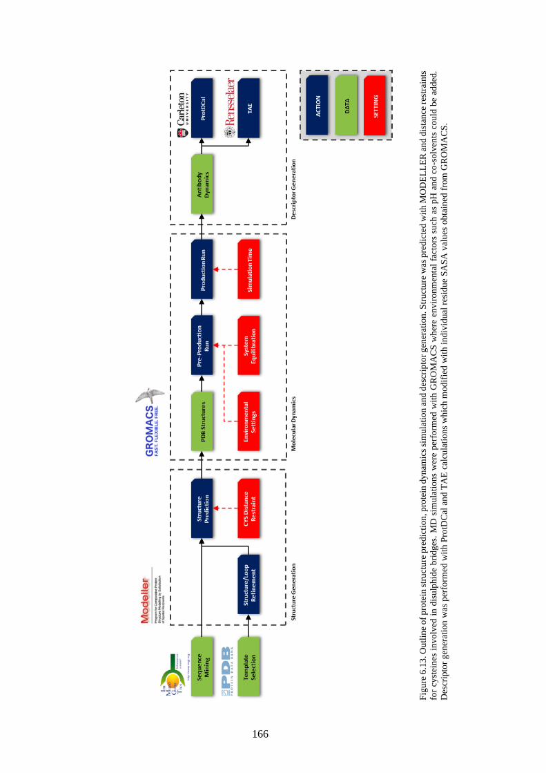
166

Fig

ure

6.1

3. O

utl

ine

of

pro

tein

str

uct

ure

pre

dic

tion

, p

rote

in d

yn

amic

s si

mu

lati

on

an

d d

escr

ipto

r g

ener

atio

n. S

tru

ctu

re w

as p

red

icte

d w

ith

MO

DE

LL

ER

an

d d

ista

nce

res

trai

nts

for

cyst

ein

es i

nv

olv

ed i

n d

isu

lph

ide

bri

dg

es.

MD

sim

ula

tio

ns

wer

e p

erfo

rmed

wit

h G

RO

MA

CS

wh

ere

env

iro

nm

enta

l fa

cto

rs s

uch

as

pH

an

d c

o-s

olv

ents

co

uld

be

add

ed.

Des

crip

tor

gen

erat

ion

was

per

form

ed w

ith

Pro

tDC

al a

nd

TA

E c

alcu

lati

on

s w

hic

h m

od

ifie

d w

ith

in

div

idu

al r

esid

ue

SA

SA

val

ues

ob

tain

ed f

rom

GR

OM

AC

S.

167

6.6.1 Time frame selection

Due to the constraints placed on the backbone in production run, relaxation of the structures

occurred in the beginning of the simulation for each mAb. This is illustrated in Figure 6.14

which shows the conformational change of adalimumab simulated in water. It can be observed

in Figure 6.14a that a conformational shift occurs from its original conformation (t=0) to a more

relaxed conformation (t=5) which is then retained throughout the rest of the simulation

indicating that an equilibrium has been reached. The RMSD used in the figure is a measurement

of atomistic deviation over time from a reference structure where the constrained structure from

the previous NPT equilibration was used. This conforms to the idea of the energy landscape

illustrated in Figure 6.3a where the protein structure will strive to attain as low conformational

energy as possible. It also illustrates the structure bias from MODELLER where the predicted

structure is biased towards the template and not necessarily in a relaxed state.

Further analysis showed that the smaller fluctuations (vibrations) observed in Figure 6.14a were

due to local motions of the loops and turns in the mAb and are illustrated as the peaks in Figure

6.14b and Figure 6.14c for the light chain and heavy chain, respectively. The RMSF values

used in the figures are temporal averages of the atomic trajectories (i.e. motions) in space of the

residues, thus capturing the residue fluctuation over time. The RMSF values in the figures were

calculated from the protein motions acquired after equilibrium had been reached until the end

of the simulation.

Based on these facts, the extraction of the structure was therefore performed by selecting a time

frame located in the equilibrium interval of the simulations. The timeframe was selected

towards the end of each simulation in order to allow the structures to relax and reach

conformational stability. This was due to the fact that relaxation times between mAbs varied,

thus introducing uncertainty of conformational stability if earlier timeframes were used. This is

covered more in detail in Section 7.1.2 which discusses the simulation results for the 137 mAbs

in the publication of Jain et al. (2017).

168

Figure 6.14. MD simulation result for adalimumab. (a) The conformational change of adalimumab evolving over

time in the production run. (b) The average fluctuations of the individual residues in the light chain between t=5

ns and t=50 ns. (c) The average fluctuations of the individual residues in the heavy chain between t=5 ns and t=50

ns.

6.6.2 Descriptor software and calculations

Similar to the primary sequence-based descriptors, ProtDCal was used for generation of 3D

structure descriptor by using the acquired PDB structures from the MD simulations as input

(Ruiz-Blanco et al., 2015). GROMACS was used to generate the solvent accessible surface area

(SASA) for the residues in the mAbs which were used as basis or modification of many of the

generated descriptors. Table 6.7 lists the descriptors. Focus was placed on descriptors pertaining

to the surface, shape and energies that were impossible to capture when using the primary

sequence.

169

Table 6.7. List of energy and topological descriptors used to describe the protein structure

Descriptor ProtDCal GROMACS Type Description

𝑮𝒄(𝑭) ● Energy Contribution to the free energy from the

conformational entropy in a folded state

𝑮𝑾(𝑭) ● Energy Contribution to the free energy from the

entropy of the first shell of water

molecules in a folded state

𝑮𝒔(𝑭) ● Energy Interfacial free energy of a folded state

𝑾(𝑭) ● Energy Number of water molecules close to a

residue in a folded state

𝑯𝑩𝒅 ● Energy Number of hydrogen bond in the

backbone of the protein

𝚫𝑮𝒔 ● Energy Variation of the interfacial free energy

between folded and unfolded states

𝚫𝑮𝑾 ● Energy Contribution to the folding free energy

of the first shell off water molecules

𝚫𝑮𝒆𝒍 ● Energy Free energy contribution of the charge

distribution within the protein

𝚫𝑮𝑳𝑱 ● Energy Contribution of the Van der Waals

interaction to the folding free energy

𝚫𝑮𝒕𝒐𝒓𝒔 ● Energy Contribution of the dihedral torsion

potential to the folding free energy

𝑺𝑨𝑺𝑨𝒑𝒐𝒍𝒂𝒓 ● Topological The total solvent accessible surface area

from the polar residues

𝑺𝒑𝒐𝒍𝒂𝒓 ● Topological The effective surface polarity from the

charged and polar residues

𝑺𝑨𝑺𝑨𝒏𝒐𝒏−𝒑𝒐𝒍𝒂𝒓 ● Topological The total solvent accessible surface area

from the non-polar residues

𝑺𝒏𝒐𝒏−𝒑𝒐𝒍𝒂𝒓 ● Topological The effective surface hydrophobicity

from the non-polar residues

𝒍𝒏(𝑭𝑫) ● Topological Logarithm of the folding degree

In addition, 37 Transferable Atom Equivalent (TAE) descriptors were used in order to describe

electron and charge densities of the mAbs. TAE is in simple terms a library of empirical atomic

charge density components that are used to construct electron densities able to describe the

protein surface of individual amino acids (Breneman and Rhem, 1997).

The TAE descriptors used in this research were available in ProtDCal as listed value for each

amino acid. This meant that the generated TAE descriptors were based on the amino acid

composition in ProtDCal rather than feature of the protein and therefore no different from using

the primary sequence as input. In order to conform these descriptors to represent the surface of

the mAb the generated SASA values from GROMACS were used according to eq.(6.21). The

equation calculates the fraction of each amino acid that is accessible to solvent and is known as

170

the relative surface area (RSA) and ranges from zero (the residue is completely buried) to one

(maximum exposure).

𝑇𝐴𝐸𝑘

𝑆𝑢𝑟𝑓𝑎𝑐𝑒= ∑

𝑆𝐴𝑆𝐴𝑖

𝑀𝑎𝑥𝐴𝑆𝐴𝑖𝑇𝐴𝐸𝑖𝑘 =

𝑖

∑𝑅𝑆𝐴𝑖 ∙ 𝑇𝐴𝐸𝑖𝑘

𝑖

(6.21)

𝑇𝐴𝐸𝑘𝑆𝑢𝑟𝑓𝑎𝑐𝑒

is the resulting 𝑘𝑡ℎ TAE descriptor for the surface, 𝑆𝐴𝑆𝐴𝑖 is the solvent accessible

surface area of residue 𝑖, 𝑀𝑎𝑥𝐴𝑆𝐴𝑖 is the maximum accessible surface area of a residue 𝑖,

𝑇𝐴𝐸𝑖𝑘 it the 𝑘𝑡ℎ listed TAE descriptor for residue 𝑖 and 𝑅𝑆𝐴𝑖 is the relative surface area of

residue 𝑖. The 𝑀𝑎𝑥𝐴𝑆𝐴 value is defined as the accessible surface area of an amino acid X in a

Gly-X-Gly tripeptide conformation. Published empirical values from Tien et al. (2013) were

used to calculate the descriptor in this research.

In a similar fashion, descriptors for describing the hydrophobicity, eq.(6.22), and the polarity,

eq.(6.23), of the surface were generated by using the Kyte-Doolittle scale. Specifically, the

hydrophobicity of the surface was calculated by using the nine in the NPR amino acid group in

Table 3.3 in Chapter 3 and the polarity was calculated using the 11 residues in the PLR amino

acid group.

𝑆𝑛𝑜𝑛−𝑝𝑜𝑙𝑎𝑟 = ∑


𝑀𝑎𝑥𝐴𝑆𝐴𝑖𝑘𝑖

𝐾𝐷

𝑖 ∈ 𝑁𝑃𝑅𝑝

(6.22)

𝑆𝑝𝑜𝑙𝑎𝑟 = ∑


𝑀𝑎𝑥𝐴𝑆𝐴𝑖𝑘𝑖

𝐾𝐷

𝑖 ∈ 𝑃𝐿𝑅𝑝

(6.23)

𝑆𝑛𝑜𝑛−𝑝𝑜𝑙𝑎𝑟is the surface descriptor describing the hydrophobicity, 𝑆𝑝𝑜𝑙𝑎𝑟is the surface

descriptor describing the surface polarity and 𝑘𝑖𝐾𝐷 is the Kyte-Doolittle value for residue 𝑖.

No treatment was needed for the generated energy descriptors from ProtDCal as these are

calculated based on the surrounding environment.

6.6.3 Descriptor resolution

Similar to the primary sequence-based descriptor, strategies for defining the descriptor

resolution was used where selection of residues to use were based on the intrinsic structural

features of all mAbs (see Section 3.3). Three different resolutions were considered when

171

generating 3D structure descriptors: Chain, Domain and Substructure. Table 6.8 lists the

number of generated descriptors for the three resolution in a VH/VL and a Fab configuration.

Table 6.8. Number of generated descriptors based on resolution type and size of the mAb.

Method VH/VL Fab Input type Descriptors per

input

Chain Skipped (1) 104 (2) Chain 52

Domain 104 (2) 208 (4) Domain 52

Substructure 728 (14) 1456 (28) Substructure 52

(1) Is identical to the domain resolution when VH/VL is used

6.7 Summary

In this chapter a workflow for generating and simulating mAb structures has been presented.

Due to the high structural similarities shared between mAbs and availability of structure

templates, the homology modelling approach with MODELLER was selected for initial

prediction of the mAb structure. However, due to the high sequence dissimilarity in the variable

regions between the predicted structure and the template it was assumed that predicted

structures would have an unfavourable energetic state and therefore not be relaxed. MD

simulations with GROMACS was therefore performed as a subsequent step after the homology

modelling in order to relax the predicted structures.

Descriptor were then generated with ProtDCal but modified with residue SASA values from

GROMACS in order to only capture the surface properties. Generated descriptors presented in

this chapter has been applied and assessed on prediction of HIC retention times and mAb yields

in Chapter 7.

173

Chapter 7

QSAR Model Development: 3D Structure

Descriptors

In Chapter 6, a workflow for the generation of novel 3D structure descriptors was presented

which provided an alternative approach to describe the mAb structure compared to the

previously explored descriptors generated from the primary sequences described in Chapter 3.

The 3D structure descriptors were designed to represent the surface properties as well as the

stability properties of the mAbs. Three different 3D structure descriptor resolutions were

investigated which were generated based on the full chains, the individual domains and the

individual substructures present in the mAb structure (from the lowest to the highest resolution).

The new 3D structure descriptors were first evaluated for potential systematic variation

originating from the unique structure of the light chain isotypes with the use of PCA. In

addition, the potential variation originating from the species origins was also explored with

classification methods such as PLS-DA and SVC. These were important factors in the

development of the predictive models presented in Chapter 5 where the primary sequence-based

descriptors contained systematic variation uncorrelated to the investigated responses.

HIC retention times and mAb yields were chosen as response vectors for model development

due to being important parameters in pharmaceutical industries for the assessment of

productivity and product stability, respectively. All models were developed according to the

benchmarking scheme first presented in Chapter 5. PLS and SVR were used as modelling

methods. Model optimisation was performed in incremental steps where V-WSP was used for

initial variable reduction. rPLS, LASSO and GA was then applied for subsequent variable

selection on the V-WSP reduced descriptor set in order to increase correlation between

descriptors and responses.

174


7.1.1 Response Data

In this research quantitative process data published by Jain et al (2017) was used to develop

predictive models for HIC retention times and mAb yields. For more details on the dataset and

experimental setup of the mAb yield and HIC, refer to Section 5.1.1. Out of the 137 available

mAbs in the data set, 131 were retained based on the reasoning discussed in Section 5.1.1.3.

7.1.2 Descriptor Data Generation

Fab fragments of the mAbs were prepared for simulation using the available sequences of the

variable domains VH and VL provided as supplementary information in the study of Jain et al

(2017). The heavy chain was prepared by attaching an IgG1 CH1 sequence obtained from allele

sequence IGHG1*01 to the provided VH domains. Similarly, the light chain was prepared by

attaching a CL domain sequence to the provided VL domains obtained from either allele

sequence IGLK1*01 (kappa) or IGLC1*01 (lambda).

Homology models were generated using MODELLER version 2.17 (Webb and Sali, 2014) with

a single template where PDB 2FGW and 7FAB were used for Fab fragments of kappa and

lambda isotypes, respectively (see Table 6.2 in Chapter 6). Pair-wise cysteines involved in

disulphide bridges were restrained where the sulphur atoms were placed at a distance of 2 Å

from each other in order to properly connect the cysteine residues. Two mAbs (muromonab and

teplizumab) were excluded in this process due to having cysteines in the CDR regions which

caused MODELLER to form incorrect disulphide bridges, thus misrepresenting the structure.

Atomistic simulations of the Fab fragments were performed with GROMACS (version 5.1.4)

and simulated in water with a concentration of 0.1 M NaCl in order to stabilise surface charges.

Prior to the production run, the system was equilibrated to a temperature of 25 oC and pressure

of 1 bar. In this research, the high-performance computing (HPC) service ROCKET at

Newcastle University was used run the production simulation. Each Fab fragment was

simulated for a total of 50 ns to allow structure to reach conformational equilibrium described

in Section 6.6.1. Atezolizumab was excluded in this process due to causing critical failures in

the simulation. Several attempts were performed to re-simulate atezolizumab but all failed due

to high system instability.

Structural descriptors for the remaining mAbs were generated based on the methodology

presented in Section 6.6 where three unique descriptor sets were obtained: Chain based

(MSD1), Domain based (MSD2) and Substructure based (MSD3) where MSD is short for

“Molecular Structure Descriptors”. In total, this resulted in 128 mAbs being selected for further

175

evaluation as listed in Table A.3 in Appendix A with corresponding experimental

measurements for HIC retention times and mAb yields.


7.1.3.1 PCA

PCA was used as an exploratory analysis tool to investigate the three descriptor sets and the

relationship between descriptors and the light chain isotypes as well as the species origins. PCA

implementation was performed using the PLS Toolbox version 8.6.1 (Eigenvector Research,

Inc). For more details on PCA, see Section 2.2.1.

7.1.3.2 PLS-DA

The NIPALS algorithm was used to develop a PLS regression model for predicting the dummy

variables generated from the class information pertaining to the species origin of the mAbs.

Discriminant Analysis (DA) was then applied to create decision thresholds in order to classify

the predictions of the developed PLS model. For more details on PLS-DA, see Section 2.3.1.

7.1.3.3 SVC

The LibSVM toolbox was used and implemented in MATLAB 2016a for SVC model

development (Chang and Lin, 2011). The C-SVM function in LibSVM was used for multiclass

classification problems. A shell script was developed to implement the OvR multiclass strategy

in SVC instead of using the default OvO strategy in LibSVM in order to reliably compare SVC

to PLS-DA. The shell scripts for model fitting and prediction are presented in Appendix B,

Code B.1 and Code B.2, respectively. Optimisation of the model parameter 𝐶 was performed

using a grid search approach on defined points over specified ranges for each parameter (for

details on parameters see Section 2.3.2). The grid points used for 𝐶 were

[10-5, 10-4, 10-3, 10-2, 10-1, 100, 101, 102, 103, 104].

7.1.3.4 PLS

Partial Least Squares regression was performed using the NIPALS algorithm. The first 20 latent

variables were calculated to allow for a majority of the data variation in 𝑿 and 𝒀 to be captured.

A higher number of latent variables is often not recommended as they usually only improve

fitting of individual samples, thus causing over-fitting (Wold et al., 2001). For more information

on PLS, refer to Section 2.4.1.

176

7.1.3.5 SVR

The optimisation of the model parameters 𝐶 and 𝜖 was performed by using a grid search

approach on defined points over specified ranges for each parameter (for details on parameters,

see Section 2.4.2). The grid points used for 𝐶 were [10-5, 10-4, 10-3, 10-2, 10-1, 100, 101, 102, 103,

104] whereas the grid points used for 𝜖 were [10-3, 10-2.5, 10-2, 10-1.5, 10-1, 10-0.5, 100, 100.5, 101].

This resulted in 90 different model parameter permutations that were evaluated in the model

cross validation.

7.1.4 Data curation and pre-treatment

An initial data curation step was performed where descriptors with a standard deviation lower

than 0.0001 were removed as they were considered to be static and thus not contributing

informational content to the model.

Both the descriptor set (𝑿 block) and the response vector (𝒀 block) were autoscaled when used

in regression models in order to allow the descriptors to influence the resulting model equally

(see Section 2.7). In classification models, only the 𝑿 block was autoscaled whereas the class

labels were assigned as zero and one in PLS-DA and minus one and one in SVC.



Prior to model development the data set was split into a calibration set and an external test set

to represent future samples. The Kennard-Stone (CADEX) algorithm was used to divide the

samples according to structural similarity based on the Euclidean distance between samples in

the descriptor space (see Section 2.5.1 for more details). 80% of the samples were retained for

model calibration and the remaining 20% were used for external testing and model validation.

7.1.5.2 Cross-Validation scheme

A repeated k-fold cross validation scheme was applied for model development where k was

chosen to be five in order to get an 80/20 sample split ratio between training and validation

samples, respectively. 20 iterations were performed to better utilise the data set and to decrease

the potential impacts of outliers in the data on the cross validation. For more information, see

Section 2.5.2.


The validation of PLS-DA and SVC models was performed using the overall error rate (ER)

and the Matthews Correlation Coefficient (MCC) based on the confusion matrices of the

177

developed models. The appropriate model complexity of the PLS-DA and SVC models was

determined through the selection of model complexity with the lowest ER in the cross

validation. For more information on the classification metrics, refer to Section 2.6.2.

All regression models were validated using the OECD guidelines for 𝑅2 and 𝑄2 for QSAR

models (Veerasamy et al., 2011, Alexander et al., 2015). The guidelines state that 𝑅2 and 𝑄2

should be greater than 0.5 and 0.6 in the cross-validation and external prediction, respectively.

In addition, the difference between 𝑅2 and 𝑄2 should not exceed 0.3. The thresholds 𝑅2 and

𝑄2 in the OECD guidelines are intended to be used for early model development to explore

potential correlation of factors and descriptors related to the modelled responses. Once

characterised, additional descriptor development and adjustments can be performed to further

improve model performance. For more information on the regression metrics, refer to Section

2.6.1.

7.1.5.4 Y-Randomisation

Y-randomisation was used to evaluate the presence of random correlation between a descriptor

set and a randomised response vector. The response vector was randomised 50 times and an

individual model was developed on each permutation. Calculated 𝑅2 and 𝑄2 values from the

50 models were then averaged. If no chance correlation is present in the descriptor set, both the

averaged 𝑅2 and 𝑄2 values will be low. For more details on Y-randomisation, refer to Section

2.6.3.

7.1.6 Variable reduction and Selection

7.1.6.1 V-WSP

The V-WSP algorithm was applied as an unsupervised variable reduction method to remove

collinear descriptors present in the 𝑿 block. Implementation of V-WSP was performed in the

same way as described in Section 5.1.5.1.

In order to avoid removal of collinear descriptors belonging to different chains, domains or

substructure, the V-WSP reduction was performed on groups of descriptors defined by the

resolution of the descriptor set. In MSD1, the groups were defined as individual chains. In

MSD2, the groups were defined as individual domains. In MSD3, the groups were defined as

individual substructures. This was done in order to avoid excessive information loss and to

represent each group individually. Reduction with V-WSP was performed prior to any

supervised variable selection method.

178

7.1.6.2 rPLS

Supervised variable selection with rPLS was performed using PLS Toolbox 8.6.1 (Eigenvector

Research Inc) together with MATLAB 2016a (Mathworks®). An initial PLS model was

developed with selected descriptors from V-WSP reduction and the latent variable with the

smallest RMSECV was selected as a starting point for the rPLS selection. For more information

on rPLS, refer to Section 2.9.1.

7.1.6.3 GA

Supervised variable selection with Genetic Algorithm (GA) was performed using PLS Toolbox

8.6.1 (Eigenvector Research Inc) together with MATLAB 2016a (Mathworks®) and PLS as

the fitness function. A population size of 100 was used and the maximum number of generations

was set to 100. The convergence for the GA algorithm was set to 50%. Default values for the

mutation rate and the ratio of kept variables in the initial models was kept as 0.5% and 30%,

respectively. For more information on GA, refer to Section 2.9.2.

7.1.6.4 LASSO

The LASSO algorithm was implemented using the function fitrlinear in MATLAB 2016a

(Mathworks®) where SVR was set as the learner and LASSO selected as the regularisation

method. A grid search was performed in the same fashion to that of SVR described in Section

5.1.5.4 in order to optimise the parameter selection.

7.2 Results and Discussion

7.2.1 Analysis of protein dynamics

The evaluation of the simulations was performed by observing the generated RMSD plots for

the 128 mAb simulations which are shown in Figure 7.1. The majority of the mAb structures

reached conformational stability after 15 ns which can be observed as the plateaus in Figure

7.1a. However, four mAb structures failed to reach conformational stability during the

simulation where the RMSD value instead kept increasing as illustrated in Figure 7.1b.

Interestingly, three of these mAbs: briakinumab, fezakinumab and tralokinumab are of lambda

conformation whereas eldelumab is of kappa conformation. It has been shown in research that

light chains of the lambda isotype in general are more unstable than kappa which might explain

why conformational stability were not reached in the simulations (Rouet et al., 2014).

179

Figure 7.1. RMSD plots of GROMACS simulations where (a) mAbs have reached conformational stability and

(b) mAbs that have not reached conformational stability.

In addition to the plots, the standard deviation of the RMSD, 𝜎𝑅𝑀𝑆𝐷, was calculated from the

snapshots obtained between 15 ns and 50 ns in the simulations according to equation (7.1).

𝜎𝑅𝑀𝑆𝐷 = (1

𝑁𝑓𝑟𝑎𝑚𝑒𝑠 − 1∑ (𝑅𝑀𝑆𝐷𝑡 − 𝐸(𝑅𝑀𝑆𝐷))

250 𝑛𝑠

𝑡=15 𝑛𝑠

)

12

(7.1)

where 𝑁𝑓𝑟𝑎𝑚𝑒𝑠 is the number of snapshots between 15 ns and 50 ns, 𝑅𝑀𝑆𝐷𝑡 is the RMSD value

at time 𝑡 and 𝐸(𝑅𝑀𝑆𝐷) is the expected value or average of the RMSD according to equation

(7.2).

𝐸(𝑅𝑀𝑆𝐷) =1

𝑁𝑓𝑟𝑎𝑚𝑒𝑠∑ 𝑅𝑀𝑆𝐷𝑡

50 𝑛𝑠

𝑡=15 𝑛𝑠

(7.2)

The 𝜎𝑅𝑀𝑆𝐷 value thus represents the variability of the RMSD curve in the simulation interval

between 15 ns and 50 ns where stability had been reached for the majority of mAb structures.

Therefore, in a more indirect manner, the 𝜎𝑅𝑀𝑆𝐷 value can be used to infer conformational

stability of a protein where a low value represents a stable conformation whereas a high value

represents conformational change. The four mAb structures: briakinumab, fezakinumab,

tralokinumab and eldelumab illustrated in Figure 7.1b had 𝜎𝑅𝑀𝑆𝐷 values above 0.12 with the

highest value of 0.21 (fezakinumab). The mAb structures that were considered stable all had

values below 0.07, thus having less conformational variation occurring after the structure had

been relaxed (data not shown). Further inspection of eldelumab was performed in order to

180

investigate the second plateau illustrated in Figure 7.1b between 30 ns and 50 ns of the

simulation. It was observed that the rise in RMSD occurring at 30 ns was caused by the VH

domain slightly twisting upwards in the Fab fragment as illustrated in Figure 7.2 where Figure

7.2a and Figure 7.2b are snapshots taken at the 25 ns and 35 ns timeframes of the simulation

respectively. The new structural conformation of eldelumab illustrated in Figure 7.2b then

remained stable throughout the rest of the simulation. In the case of briakinumab, fezakinumab

and tralokinumab, twisting occurred in all domains where the VH and VL domains packed closer

to the CL and CH1 domains respectively, thus resulting in a more compact and spherical

structure (data not shown). The observed conformational change of the structures were gradual

throughout the simulations which also explains the continued increase of the RMSD values for

briakinumab, fezakinumab and tralokinumab.

Figure 7.2. Displacement of the VH domain (blue arrow) in the simulation of eldelumab from the domains original

position captured at (a) 25 ns to its new placement captured at (b) 35 ns. The heavy chain is coloured blue while

the light chain is coloured red.

For all simulations except briakinumab, eldelumab, fezakinumab and tralokinumab, the

structures remained stable throughout the simulation and no conformational changes occurred.

The last timeframe in each of these simulations was therefore used to generate a PDB structure

from which descriptors were later generated (see Section 6.6). For eldelumab, the last timeframe

was used due to that the second plateau remained stable from 30 ns until the end of the

simulation. Preferably, continued simulation of briakinumab, fezakinumab and tralokinumab

would be desirable in order to allow the structures to converge to a stable conformation.

However, due to time constraints within the project, the last timeframe in the simulations (50

ns) were used to generate the descriptors. Though it introduces some uncertainty regarding

181

briakinumab, fezakinumab and tralokinumab structural stability, it was believed that if the

simulations were allowed to run further, they would converge to a stable conformation.

Therefore by selecting the last timeframe in the simulation, it could be assumed that the

structures would be closer to the stable conformations than they were prior to the simulations.

7.2.2 Impact of the light chain isotypes

Similar to the exploratory analysis performed in Chapter 4 on the 273 mAb sequences obtained

from the IMGT database, the impact of the light chain isotypes, kappa and lambda, on the

generated 3D structure descriptors described in Chapter 6 was explored with PCA. Only

descriptors generated from the light chain were used in this exploratory analysis because no

structural information relating to the heavy chain isotype were present in the structures due to

all mAbs being expressed as IgG1. The number of principal components (PCs) was

incrementally increased until approximately 90% of the data variation in the descriptors sets

had been explained. This was done due to the light chain isotype being expected to have a strong

impact on the generated descriptors in a similar fashion as was observed in Chapter 4 for the

primary sequence-based descriptors.

A clear diagonal separation of kappa and lambda could be observed in the first and second PCs

in MSD1 (Figure 7.3a), MSD2 (Figure 7.3b) and MSD3 (Figure 7.3c) with an explained

variation of 81.18%, 72.0.3% and 42.45%, respectively. However, not all of the explained

variation of the first two PCs can be attributed entirely to the separation of the isotypes which

also separates the individual samples from each other due to their unique surface properties. It

is difficult to estimate to what extent the VL and CL domains influence the separation. However,

a clear contribution from both domains could be observed when investigating the loadings of

PC1 and PC2, as illustrated in Figure C.7 in Appendix C. The remaining PCs showed no further

separation of the light chain isotypes and were therefore assumed to capture variation related to

individual samples instead (data not shown). A short summary of the PCA results is presented

in Table 7.1.

The statistical analysis on the response vectors of the HIC retention time and mAb yield

performed in Section 5.2.2 is still valid due to being independent from the generated descriptors

and only investigates the behaviour of the responses according to the isotypes. Just as with the

primary sequence-based descriptors, a strong impact of the isotypes on the generated 3D

structure descriptors was evident (see Figure 7.3). This can potentially act as a systematic

variation that is uncorrelated to the response and can have a negative impact on the performance

of developed regression models (Wold et al., 1998). It is important to remember that the heavy

chain was modified by Jain et al (2017) where all heavy chain constant domains were expressed

182

as IgG1 regardless of their original conformation. Therefore, no conclusions can be drawn with

regards to the impact of the original heavy chain isotypes on the responses. For these reasons,

only IgG1-kappa samples were used for further model development, resulting in 79 samples

being retained from the previously 128 selected samples.

As previously described in Chapter 4, the amino acid composition of the primary sequence in

the VL domain will be different between kappa and lambda due to being expressed from

separate genes in the VJ recombination (Jung and Alt, 2004). This had a significant impact on

the generated 3D structure descriptors from the VL domain which had high contributions to the

loadings of the PC1 and PC2 (see Figure C.7 in Appendix C). This indicates that a fraction of

residues directly related to the light chain isotype are present on the surface and it further

highlights the need for an appropriate selection of samples in order to avoid introduction of

uncorrelated systematic variation prior to model development.

Figure 7.3. PCA score plots of the first two components calculated from the light chain descriptors from MSD1

(a), MSD2 (b) and MSD3 (c) where kappa and lambda samples are coloured red and green, respectively.

183

Table 7.1. PCA exploration summary of light chain descriptors from MSD1, MSD2 and MSD3 where each model

was developed to capture approximately 90% of the total data variation. The last two columns show information

of PCs related to the LC isotype separation and the cumulative explained variation of those PCs.

Descriptor

Set

Number of

Descriptors

Principal

Components

Explained

Variation (%)

LC Isotype

separating

components

Explained

Variation (%) by

selected component

MSD1 50 4 90.04 1 and 2 81.18

MSD2 100 6 90.24 1 and 2 72.03

MSD3 632 26 90.12 1 and 2 42.45

7.2.3 Impact of species origin

To explore the potential impact of the species origin, classification methods such as PLS-DA

and SVC were applied to the 79 selected IgG1-kappa samples. All 100 descriptors in MSD1

were used in the model development due to having been calculated on the full heavy or light

chains where separation of constant and variable domains is not possible (see Section 6.6.3).

As for MSD2 and MSD3, only descriptors belonging to the variable domains VH and VL were

used which resulted in 100 and 644 descriptors being used, respectively. The CADEX algorithm

was used to split the data into 80/20 for calibration and test, respectively, according to the

structural information contained in the individual descriptor sets MSD1, MSD2 and MSD3.

When CADEX was used directly, the algorithm produced a skewed split of species origins in

the calibration and test sets in all individual descriptor sets. This was especially pronounced for

the chimeric species origin where only one sample was placed in the test set for MSD2 and

MSD3 while no samples were placed in the test set for MSD1. Instead, a sample stratification

strategy was implemented to ensure that all species origins were appropriately represented in

the test set (Shahrokh and Dougherty, 2013). This was performed by applying the CADEX

algorithm individually on the three species origins where 80% were retained for training and

20% for model validation in the test set. A summary of the sample splitting is presented in Table

C.6 in Appendix C.

A summary of the performance of the developed PLS-DA and SVC models is presented in

Table 7.2 for the three descriptor sets. None of the developed models performed well in the

cross-validation where the error rates were close to 0.4 regardless of modelling method or

descriptor set, meaning that approximately 40% of the samples were classified incorrectly. The

corresponding MCC values showed an indication of a weak correlation (0.2-0.3) between the

generated descriptors and the species origin classes, thus indicating a lack of correlation in the

data (Jurman et al., 2012). This is further supported through investigation of the individual AUC

values of the three species origins obtained from the ROC curves illustrated in Figure C.8 in

184

Appendix C. For both PLS-DA and SVC models developed on the MSD1 and MSD2 descriptor

sets, the AUC values tended to be placed around 0.65 for the chimeric and human species

origins while the humanised species origin was around 0.75. For PLS-DA and SVC models

developed on the MSD3 descriptor set, the AUC value of the chimeric species origin tended to

be around 0.8 while the human and humanised classes had values around 0.7. The AUC values

are considered to be relative and dependent on the data set used. However, as a rule of thumb

AUC values above 0.8 can be considered as a reasonable performance while values below 0.8

can be considered poor (Fawcett, 2006). Thus, none of the developed classification models were

able to identify an underlaying correlation between the generated 3D structure descriptors and

the species origins.

Compared to the cross-validation, the results observed in the test set tended to vary a bit more.

In general, SVC models tended to have slightly higher MCC values and lower ER values

compared to PLS-DA. The best performance was observed in the SVC model developed on

the MSD3 descriptor set with a MCC value of 0.75 and an ER value of 0.18. However, due to

the poor performance in cross-validation this model cannot be considered to produce accurate

predictions in future samples.

Table 7.2. Summary of PLS-DA and SVC model performance developed on the descriptor sets: MSD1, MSD2,

and MSD3. The MCC and ER performance metrics for calibration (Cal), cross-validation (CV) and the external

test (Test) set are provided as well as the explained data variation of 𝑿 and 𝒀 by PLS-DA.

Method Descriptor

Set

Explained 𝑿

Variation (%)

Explained 𝒀

Variation (%)

Cal CV Test

MCC ER MCC ER MCC ER

PLS-DA

MSD1 86.68 62.27 0.86 0.08 0.19 0.48 0.29 0.41

MSD2 76.59 45.97 0.72 0.16 0.20 0.48 0.07 0.53

MSD3 26.95 57.52 0.78 0.13 0.26 0.42 0.59 0.24

SVC

MSD1 - - 0.89 0.06 0.28 0.40 0.48 0.29

MSD2 - - 0.92 0.05 0.32 0.37 0.37 0.35

MSD3 - - 0.97 0.02 0.26 0.40 0.75 0.18

When compared to the classification results in Section 4.2.5 where primary sequence-based

descriptors had a strong correlation to the species origin classes, the 3D structure descriptors

investigated in this chapter could not be directly linked to the species origin. A plausible cause

for this could be that the necessary information needed for a reliable classification becomes

buried inside the protein structure. Compared to the primary sequence-based descriptors, where

each residue in the VH and VL domains had equal representation, in the 3D structure descriptors

the species origin related residues might no longer be represented due to having been modified

to conform to the solvent accessible surface area. Thus, the systematic variation related to the

185

species origins observed in Section 4.2.5 becomes nearly negligible when 3D structure

descriptors are used.

It is important to note that there was no significant statistical difference between the means of

the HIC retention time between the three species origins whereas for the mAb yields, a

significant statistical difference between the means of the chimeric and humanised samples was

observed (see Section 5.2.2). However, due to the lack of systematic variation present in the 3D

structure descriptors related to the species origin, all 79 IgG1-kappa samples were retained for

further model development presented in Table A.3 in Appendix A.

7.2.4 HIC model development on IgG1-kappa samples

The same structured approach for model benchmarking described in Chapter 5 was applied for

regression fitting with regards to the HIC retention times. The CADEX algorithm was used to

divide the 79 retained IgG1-kappa samples into a calibration set for training (80%) and a test

set for model validation (20%). PLS and SVR were used as modelling methods. A first set of

initial models was developed on all available descriptors in MSD1, MSD2 and MSD3. A second

set of models was developed with collinearity reduction using the V-WSP algorithm to reduce

the number of descriptors in MSD1, DS and MSD3. Lastly, a final set of models was developed

on the retained descriptors from the V-WSP reduction using rPLS, LASSO and GA for variable

selection to reduce the number of descriptors even further. The model quality metrics on cross

validation and test set validations for all developed models are presented in Table C.7a in

Appendix C. These were benchmarked according to the OECD guidelines.

Models developed on the MSD1 never attained good performance and the cross-validation of

𝑅2 and 𝑄2 remained below or around 0.2 regardless of the modelling method or the level of

reduction of the descriptors. Models developed on MSD2 followed a similar trend as MSD1

but had slightly increased 𝑅2 and 𝑄2 values of 0.39 and 0.34, respectively, in PLS whereas

values of 0.30 and 0.29 were obtained in SVR after variable selection with GA. Adequate cross-

validation performance was first observed when models were developed on MSD3 in the

following cases: 1) PLS model after descriptor selection with rPLS, 2) PLS model after

descriptor selection with GA and 3) SVR model after descriptor selection with GA. Out of these

three, only descriptor selection with GA demonstrated satisfactory performance in the external

test with a 𝑅2 and 𝑄2 of 0.66 and 0.65, respectively, for PLS and a 𝑅2 and 𝑄2 of 0.64 and 0.63,

respectively, for SVR. Neither rPLS nor LASSO performed as well as GA for variable selection

on the MSD3 descriptor set. LASSO especially had poor performance in both the cross-

validation and test set whereas rPLS had acceptable performance in terms of the OECD

guidelines in the cross-validation but poor performance in the test set. A potential cause to this

186

might be due to the descriptor sets containing redundant descriptors with differing levels of

collinearity toward response correlated descriptors. Especially for the LASSO algorithm to

work properly, only a small degree of collinearity can exist between redundant and response

correlated descriptors in order for the appropriate selection to be performed (Meinshausen and

Yu, 2009). In conclusion, only the PLS and SVR models developed using MSD3 (Substructure

based) and optimised with GA fulfilled the OECD criteria for both cross validation (𝑅2 and

𝑄2 > 0.5) and external testing (𝑅2 and 𝑄2 > 0.6) (Veerasamy et al., 2011, Alexander et al.,

2015). Due to similar model performance, both the PLS and SVR models can be used for the

prediction of HIC retention times. However, the PLS model is preferred in an industrial setting

due to being more straightforward to train where only one model parameter needs to be

specified. The PLS model also have stronger diagnostic capabilities where the investigation of

sample and descriptor contribution towards 𝒀 is more intuitive.

The selected model was developed initially from the original 1163 descriptors available in the

full MSD3 descriptor set where 319 were retained from the V-WSP reduction, thus effectively

reducing the number of descriptors by ~70%. The Procrustes index was used to evaluate the

loss of information when comparing the full and V-WSP reduced MSD3 descriptor sets. A

value of 0.0638 was obtained, indicating that only a small fraction of the information was lost

in the reduction step (Ballabio et al., 2014). This can also be observed in benchmark table for

MSD3 (see Table C3.2a in Appendix C) where the of 𝑅2 and 𝑄2 values in the cross validation

and the test set remained mostly unchanged after the reduction. Out of the 319 remaining

descriptors, GA selected a subset of 51 descriptors used to develop the final PLS model. A full

list of the selected descriptors is presented in Table C.8 in Appendix C. Model predictions of

the calibration samples (dark circles) and test samples (red circles) are shown in Figure 7.4a as

a measured vs predicted parity plot. The test samples from Figure 7.4a are further illustrated in

Figure 7.4b as a bar plot for easier comparison of the measured and predicted values for

individual mAbs. The model performance is summarised in Table 7.3.

Y-Randomisation (or Y-Scrambling) was used as a final validation step to evaluate the selection

of the descriptors (Rücker et al., 2007). A PLS model was trained on a randomised (scrambled)

HIC response vector while the sample order in the MSD3 descriptor set was kept unchanged.

This was repeated 50 times and the average of 𝑅2 and 𝑄2 for the cross validation was calculated.

A resulting 𝑅2 value of 0.03 and a 𝑄2 value of -3.94 was obtained. This indicates that no chance

correlation is captured by the model and that the selected descriptors are important to describe

the relationship between the structure of the mAbs and HIC responses. The results are

summarised in Table 7.3.

187

Figure 7.4. Predictions of HIC retention times with PLS-GA model developed on the MSD3 descriptor set (LVs

= 9). (a) Measured versus predicted plot with calibration samples in black and test set samples in red. (b) Measured

(black) and predicted (red) values of test set samples.

Table 7.3. PLS model summary developed for HIC retention time prediction using the MSD3 descriptor set. Root

Mean Square Error (RMSE), R2, Q2 and model bias are listed for Calibration, Cross validation, Test set and Y-

randomisation (Y-scrambled). The Y-randomisation metrics are the average values of 50 randomised models.

PLS

RMSE R2 Q2 Bias

Calibration 0.13 0.98 0.98 0.00

Cross Validation 0.51 0.75 0.71 0.02

Test 0.59 0.66 0.65 -0.11

Y-scrambled

(Average) 2.01 0.03 -3.94 -0.01

The developed PLS model has signs of slight over-fitting when observing the calibration

samples (dark) and the test set samples (red) in Figure 7.4a. The calibration samples showed a

low RMSE value of 0.13 compared to the test set with an RMSE value of 0.59, which is also

indicated by a greater distance of these samples from the parity line. This is an indication of

over-fitting as the RMSE values between the calibration and test set should be ideally similar

to each other (Lever et al., 2016). A likely reason for this is that a small number of redundant

or noisy descriptors were selected by the GA algorithm to better fit the calibration samples in

the cross-validation which in turn resulted in a high calibration fit with 𝑅2 and 𝑄2 values of

0.98 and 0.98, respectively (Leardi, 2000). However, though not perfect, the underlaying

correlation between the mAb structures and the HIC retention times has been captured by the

PLS model as indicated by 𝑅2 and 𝑄2 values greater than 0.6 for the test set (Veerasamy et al.,

2011)

188

A general trend observed in the descriptors was that about 45% of all descriptor belonged to

the CDR regions, 31% to the framework regions and the remaining 24% belonged to both the

constant domains of CH1 and CL (see Table C.8 in Appendix C). This indicates the importance

of the structural information contained in the variable domains. This is sensible as the CDRs

are the source of the greatest sequence variability in the entire mAb structure which in turn

affects surface and structure related properties of both the CDRs as well as framework regions

in the variable domains (Lefranc et al., 2003). The effect will likely not be as pronounced in the

constant domains of the 79 IgG1-kappa samples due to having identical primary sequence.

Instead, the variability present in the 3D structure descriptors of the constant domains are likely

to be related to conformational differences originating from the molecular dynamics

simulations. However, it is important to note that the descriptors from the constant domains

cannot be disregarded due to dynamic interactions between the constant and variable domains

which in turn will affect the generated descriptors (Feige et al., 2010).

A closer inspection of the descriptors revealed that selected descriptors describing the polar

surface areas (Spolar and SASApolar) and non-polar surface areas (Snon-polar and SASAnon-polar)

belonged almost exclusively to the CDR regions. Representation of the volume (VOLTAE) and

the electrostatic potential (SIEP) generated as part of the TAE descriptors were also commonly

found belonging to the CDRs. This is consistent with published research where the CDRs have

a pivotal role in binding to the HIC column resin with stronger binding usually occurring when

the CDRs are long and hydrophobic (Hebditch et al., 2018).

In addition, the stability of the mAb structures played a central role for prediction of the

retention times represented mostly by energy-based descriptors. 11 of the 24 GA selected

energy descriptors were related to the conformational entropy Gc(F), which describes the

stability of the protein with regards to the hydrophobic interactions in the protein core which

were selected for the CDRs, framework regions and the constant domains. Other important

energy descriptors of note were the number of estimated water molecules surrounding the

surface, W(F), and the interfacial free energy, ΔGs, representing the energy contribution from

interactions between polar residues and surrounding water molecules. This is supported by

published literature where the protein stability has been reported to play a pivotal role in HIC

binding (Beyer and Jungbauer, 2018). This is further elucidated when considering that salt is

added to promote binding in HIC columns and more stable mAbs require higher concentration

of salt to disrupt electrostatic forces on the surface in order to expose hydrophobic patches

(Gagnon, 1996a).

189

In retrospect, a replacement for the TAE descriptors might help to improve model performance.

This is due to the TAE descriptors consisting of static values for the individual amino acids

which will be identical regardless of the environment they are in (Breneman and Rhem, 1997).

Similarly, an alternative to the ProtDCal descriptors describing the energy and stability of the

structure might also improve model performance due to being based on simplified empirical

calculations. It was shown that they can provide a fair and often good approximation of stability

energies when compared to experimental results. However, their applicability was not suited

for all protein structures where large differences were observed between predicted and observed

experimental energies in some cases (Ruiz-Blanco et al., 2013). A suggestion would be to

perform surface properties and energy calculations directly in GROMACS or similar software

as will be discussed further in Section 8.1.

7.2.5 mAb yield model development on IgG1-kappa samples

An identical benchmarking scheme as described at the start of Section 7.2.4 was performed to

fit the MSD1, MSD2 and MSD3 descriptor sets to the mAb yield response. The cross validation

and test set validation for all developed models are presented in Appendix C, Table C.7b. The

developed models behaved similarly to the models for the prediction of the HIC retention times,

where adequate performance in the cross validation was only achieved after variable selection

had been performed. GA selection and rPLS achieved acceptable performance with 𝑅2 and 𝑄2

greater than 0.6 for both PLS and SVR developed using MSD3 descriptor set. Selection with

LASSO however suffered due to correlation between redundant and response-correlated

descriptors as explained in Section 2.9.3.

Unfortunately, none of the developed models had an adequate performance in the external test

set regardless of which permutation of modelling, reduction or variable selection method was

used. The predictions from the PLS model developed using MSD3 and optimised with GA is

illustrated in Figure 7.5a. The test samples (red circles) from Figure 7.5a are further illustrated

in Figure 7.5b as a bar plot for easier comparison of the measured and predicted values for

individual mAbs.It can be observed that many of the test set samples have been underpredicted

which resulted in low 𝑅2 and 𝑄2 values of 0.11 and -0.92, respectively. The model performance

is summarised in Table 7.4.

190

Figure 7.5. Predictions of mAb yield with a PLS-GA model developed on the MSD3 descriptor set (LVs = 3). (a)

Measured versus predicted plot with calibration samples (black) and test set samples (red). (b) Measured (black)

and predicted (red) values of test set samples.

Table 7.4. PLS model summary developed for mAb yield prediction using the MSD3 descriptor set. Root Mean

Square Error (RMSE), R2, Q2 and model bias are listed for Calibration, Cross validation and Test set.

PLS

RMSE R2 Q2 Bias

Calibration 20.09 0.90 0.90 0

Cross Validation 36.42 0.69 0.68 -2.73

Test 74.25 0.11 -0.92 49.55

It is difficult to identify the true reason for the poor performance in the test set although a

potential cause may be the lack of necessary variation in the data. Addition of extra samples to

the data set might aid to better represent the range of 𝒀 responses, but also to introduce more

structural variation in the 𝑿 block. Noise and descriptor collinearity are also influencing factors

in the model development where the descriptor selection methods can suffer where the wrong

descriptors are selected thus leading to fitting of noise uncorrelated to the samples in the test

set (Fan and Lv, 2010). A nested cross-validation approach might help in improving the model

generalisation due to using all the available data but at the loss of a dedicated test set (Cawley

and Talbot, 2010). Another approach would be to try ensemble techniques such as bagging or

boosting where multiple models are developed on separate sample subsets which have been

shown to improve model performance and generalisation (Drucker, 1997).

From a more biological perspective, transcription and translation of the heavy and light chains

occurs separately within the cell which usually result in a higher concentration of light chains

being expressed compared to the heavy chains. The structure of the mAbs might therefore not

be directly related to the mAb yields (Bayat et al., 2018, Bhoskar et al., 2013). In Pybus et al.

(2014), the authors investigated the mAb expression with regards to the corresponding mRNA

191

structure in CHO cells. They found that expression was significantly impacted by the stability

of the mRNA structure where less stable mRNA structures resulted in lower yields. The mRNA

sequence also determines which RNA codons are used during translation which has a

significant impact on the expression as also reported by the authors. Optimisation of the

nucleotide sequence is therefore vital in order to have an efficient expression of mAbs. The

sequence variation in the variable domains has also been shown to impact expression in CHO

cells which relates back to the mRNA and RNA codons (Mason et al., 2012). The sequence

variation can impact the protein folding in the endoplasmic reticulum which in turn can become

overloaded due to the accumulation of unfolded or misfolded proteins, thus leading to lower

expression rates (Braakman and Bulleid, 2011, Stoops et al., 2012). Based on these facts, it is

therefore difficult to accurately predict the yields based on the mAb structure alone, but

information pertaining to the mRNA sequences would be needed as well (Pybus et al., 2014).

7.2.6 Comparison to primary sequence-based models

Initially, a model comparison for HIC retention time prediction of the developed primary

sequence-based model presented in Section 5.2.3 and the developed 3D structure model

presented in Section 7.2.4 was supposed to be performed with an independent external data set.

Due to using CADEX, different samples were selected for the test set in the two models which

meant that an unbiased evaluation using the samples from the data set provided by Jain et al.

(2017) could not be performed. Instead, HIC retention times for humanised mAbs from the

Advanced Manufacturing Supply Chain Initiative (AMSCI) data were supposed to be used

(CPI, 2015). However, due to project time constraint and the lengthy process to draw up

confidentiality agreements, the AMSCI sequences and HIC retention times could not be

accessed in time and a direct comparison between the models was therefore no longer possible.

However, some conclusions regarding the applicability can be made. As was observed in

Chapter 5, when all species origins were used in model development, none of the resulting

models had adequate performance with regards to the OECD criteria due to poor performance

in the test set (𝑅2 and 𝑄2 < 0.6). This was caused by the systematic variation in the primary

sequence-based descriptors that originated from structural differences between the species

origins which were uncorrelated to the HIC response (see Section 5.2.2). Adequate performance

was not reached until only humanised samples had been selected, significantly increasing the

model performance in both the cross validation and test set when primary sequence-based

descriptors were used. In comparison, due to the negligible systematic variation present in the

generated 3D structure descriptors from the species origins, model development could proceed

with all available IgG1-kappa samples as well as achieving adequate performance in both the

192

cross-validation and test set (see Section 7.2.4). The use of 3D structure descriptors therefore

increases the applicability of the QSAR model to the point where the species origin can be

ignored. However, stronger systematic variations originating from the different mab isotypes

still needs to be considered and therefore the model will only be able to predict accurately on

IgG1-Kappa samples.

From the perspective of a pharmaceutical industry, neither the primary sequence-based model

or the 3D structure descriptor model has adequate performance to be used as a predictive tool

in QbD risk assessment as of yet. This would require a higher model performance with 𝑅2 and

𝑄2 values of at least 0.8 in both the cross-validation and test set in order to decrease the offset

between measured and predicted values thus increasing the confidence in the predictions.

However, based on the acquired results, both the primary sequence-based descriptors and the

3D structure descriptors shows promise for further improvements. In this research, the initial

descriptor sets were developed to capture a wide range of different properties and features in

although the majority of these were discarded in the model optimisation with V-WSP reduction

and GA selection. Further model development is therefore recommended by re-evaluating the

properties of the selected descriptors in order to expand and incorporate more related structural

properties and features in the descriptor sets. It is important to note that the 3D structure

descriptors are more flexible than the primary sequence-based descriptors. This is due to that

process related information regarding the environment e.g. temperature, pH, molality etc can

be incorporated in the MD simulations and their effects on the protein structure can be

approximated (see Section 6.5). This is not possible with the primary sequence-based

descriptors due to being static.

7.3 Summary

In this chapter the 3D structure descriptors, developed from mAb structures simulated with

GROMACS, were explored and used for the development of predictive models for the

prediction of HIC retention times and mAb yields.

Exploration of the 3D structure descriptors of the light chain with PCA showed a strong

correlation to the kappa and lambda isotypes which were present in all of the three generated

descriptor sets. Based on previous results from the statistical hypothesis testing in Section 5.2.2,

no correlation between the light chain isotypes and responses of HIC retention times as well as

mAb yields could be significantly proven. As described in Section 7.1.1, modification of the

heavy chain was made by Jain et al (2017) as they expressed all IgG2 and IgG4 mAbs as IgG1.

If the original isotypes were preserved, though unknown, it could have potentially altered the

measured experimental responses. For this reason, only IgG1 samples were selected due to the

193

uncertainty of the true behaviour of the IgG2 and IgG4 mAbs. Contrary to the previously

explored primary sequence-based descriptors, only negligible correlation between the

generated 3D structure descriptors and the species origins was observed through classification

models based on PLS-DA and SVC. As a result, selection of a subset of 79 IgG1-kappa samples

of all species origins from the available 128 samples was used in order to reduce harmful

systematic variation uncorrelated to the response vectors as well as keeping the samples true to

their original conformations.

In this chapter, it has been shown that a model for predicting the HIC retention times could be

developed with 3D structure descriptors generated from the individual substructures (MSD3)

of a Fab fragment. Both PLS and SVR models developed on the MSD3 descriptor set after

descriptor selection with GA had similar performance, but the PLS model was selected due to

more straightforward implementation. The PLS model had adequate performance in accordance

with the OECD guidelines for QSAR models with a 𝑅2 and 𝑄2 of 0.75 and 0.71, respectively,

in the cross validation and a 𝑅2 and 𝑄2 of 0.66 and 0.65, respectively, in the test set. Though

not all variation was explained by the model, it provided valuable insight into important

descriptors and factors affecting model performance.

No satisfactory model could be developed for the prediction of mAb yields as indicated by the

signs of overfitting evidenced by the poor test set results. A potential cause could be that

structural information alone might not be directly correlated to the yield and other factors

related to the expression from the cell might be missing.

Unfortunately, no direct comparison could be made between the selected primary sequence-

based model in Chapter 5 and the 3D structure model in this chapter for prediction of HIC

retention times as explained above. However, the model developed using the 3D structure

descriptors showed broader applicability due to being unconstrained in regards to the species

origins. In comparison, the model developed on the primary sequence-based descriptors was

trained on humanised samples only and would not be able to reliably predict retention times for

chimeric and human samples. Further improvement of the developed models is still necessary

in order to increase prediction accuracy prior to application in risk assessment.

195

Chapter 8

Conclusions and Future Work

In this project the QbD framework was reviewed due to being commonly used in process

development for mAbs and provides a systematic approach to increases process understanding

through characterisation of process parameters and their effect on the product quality. However,

due to the numerous process parameters that need to be characterised, the QbD framework still

faces challenges in implementation. Much research has been focused in areas such as high-

throughput platforms and process optimisation to reduce attrition in the process development.

However, it was identified that one of the biggest challenges in QbD implementation is the lack

of knowledge about both the process and product in early process development where the

manufacturability of an mAb might not be possible.

In the literature review, it was shown that the QSAR framework for in silico model development

has become increasingly popular for end point predictions of protein behaviour in different unit

operations. This makes the QSAR framework a potentially valuable tool which can aid risk

assessment in early process development to better direct experimental designs and thus reduce

costs. The use of in silico approaches therefore allows for more informed estimates of the

potential behaviour of a mAb in different unit operations of the process. This could become

possible by efficiently making use of historic prosses data from previously established mAb

manufacturing processes and constructing an expert system. The integration of QSAR into the

QbD framework was therefore proposed in order to increase product understanding which is

especially important in early process development.

In this research, an extensive framework was developed based on QSAR in order to address the

challenges facing mAb process development. The framework can roughly be divided into three

parts according to: 1) Generation of descriptors relating both to the primary sequence as well

as the 3D structure of mAbs. 2) Exploration and statistical assessment of generated descriptor

and responses, respectively, for elimination of detrimental systematic variation. 3) Model

196

development and validation coupled with descriptor reduction and selection. The

implementation of such frameworks is becoming increasingly important in pharmaceutical

industries in order to speed up development and lower the costs of new biopharmaceuticals.

Due to the shifts toward high-throughput technology that has occurred during the recent years

in both upstream and downstream of the mAb process, the increased availability of process data

introduces and excellent starting point for the implementation of the presented framework.

In this research, focus was placed on the development of predictive models assessing HIC

retention times and mAb yields due to these important factors for protein stability and

productivity assessment in process development. The highlights from the different chapters in

this thesis and potential improvements are addressed according to the following areas: 1)

Descriptors, 2) Sample Selection and 3) Model Development and Assessment for easier

evaluation.

8.1 Descriptors

Two different approaches for generating descriptors for development of predictive models was

reviewed and implemented in this project. The first approach presented in Chapter 3, used the

primary sequence of the mAbs where descriptors were produced using EMBOSS Pepstats,

ProtDCal and amino acid scales. These descriptors were designed to capture structural

variations based on differences in amino acid compositions between mAbs. The second

approach presented in Chapter 6, was based on development of 3D structure from the primary

sequences. Due to the lack of published structures, homology modelling was applied to produce

approximations of the 3D structures for all mAbs used in this research. Molecular Dynamics

simulations was then performed to relax the homology structures. Descriptors were then

developed with GROMACS and ProtDCal and captured properties related to the surface and

stability of the mAbs.

In both approaches, descriptor sets of different resolutions were generated. For the primary

sequence-based descriptors, the lowest resolution was attained when descriptors were

calculated from all residues in an individual domain which meant that each domain could be

represented individually. The highest resolution was attained when descriptors were generated

for each individual residue in the primary sequence. For the 3D structure descriptors, the lowest

resolution was calculated from each individual chain while the highest was calculated from the

individual substructures present in the mAb structure. By comparing the different resolutions

in the developed predictive models, a trade-off could be made in order to investigate the

required resolution for adequate model performance. More explicitly, a too low resolution

would often confound important structural properties while to high resolution would introduce

197

noise in the form of redundant descriptors into the developed models where in both cases lead

to poor model performance.

8.1.1 Suggestion for Improvements

One of the biggest weaknesses with the generated descriptors is the absence of data on protein

modifications such as the mAb glycan structure which has a major impact on the mAb stability.

Due to that the upstream environment was identical for all mAbs in data set acquired from Jain

et al. (2017), it was assumed that the glycan structure would be similar between the mAbs used

for model development in this research. However, this assumption cannot be made in an

industrial setting where the glycan structure is likely to be different between mAbs and therefore

must be considered as a source of variability and represented in the modelling data.

In this research atomistic simulations using GROMACS were performed on all mAbs in order

to relax the structure and capture the structure dynamics. However, as presented in Section

7.2.1, three mAbs failed to converge to a stable conformation. It was suggested that continued

simulation would be necessary in order for the structure to converge to a stable conformation.

In retrospect, a longer simulation time, such as 100 ns as well as multiple runs for each structure,

would be beneficial for all structures as it allows for more structural variation to be captured

while at the same time minimises the risk of simulations ending at conformational transition

points. However, running all simulations at atomistic resolution for 50 ns takes considerable

amounts of time. An alternative would be to investigate coarse-grained simulations which will

run much faster due to the protein structure being simplified thus resulting in less particles in

the simulation system. A comparison would need to be made to ensure that the protein dynamics

of coarse-grained simulation is representative to that of the atomistic simulation in order to not

bias the resulting structure. The use of coarse-grained simulation would also allow for longer

simulations to be run, thus generating a stronger foundation for understanding to structure

dynamics.

3D structure descriptor in this research were generated from a PDB structure acquired from a

single time-frame from the MD simulation. However, due to the structure being dynamic and

changing slightly over time, only using single time-frame might not accurately represent the

surface and stability of the structure. An alternative would be to generate descriptors on all

available time frames from when the structure has reached conformational stability to the end

of the simulation and then average the descriptors over time. This would probably result in

more stable and representative descriptors due to conforming to the dynamics of the mAb

structure.

198

As mentioned earlier in Chapter 7, the calculation of energy descriptor through ProtDCal are

based on simplified empirical mathematical models which might not accurately represent the

environment in which the mAbs are simulated. It is therefore proposed that stability and energy

related descriptors are calculated directly in GROMACS or equivalent software which can take

into consideration many different interactions between the atoms in the system. GROMACS

also supports energy calculations of predefined groups of residues, thus allowing for calculation

of descriptors conforming to the different descriptor set resolutions presented in Chapter 6.

Though never implemented, a workflow of modifying the titration states of residues in the mAb

structure as well as adding co-solvents to the system was presented in Chapter 6. It would be

interesting to see how the descriptors change in response to the change in pH and co-solvent

concentration. If the HIC elution curves were available for the mAbs in Jain et al. (2017) instead

of just the end point retention times, several simulations with differing salt concentrations could

have been performed and linked to the cumulative elution, thus expanding the data set.

Alternatively, the proposed methodology could be used on published experimental data which

follows DoE experimental design.

8.2 Sample Selection

Selection of samples played a critical role in the model development in order to reduce

systematic variation uncorrelated to the response vectors where a structured approach for

investigating sources of variation was proposed. Two sources of variation were identified early

on where the first originated from the unique structures of the heavy chain isotypes IgG1, IgG2

and IgG4 whereas the second originated from the unique structure of the light chain isotype

kappa and lambda. Exploration of the primary sequence-based descriptor with PCA on the

gathered 273 IMGT sequences presented in Chapter 4 revealed that both the heavy and light

chain isotypes had a clear and strong separation. Further analysis showed that a significant

portion of the data variation in the descriptors were used to explain the observed separations.

Similar results were observed when exploring the 3D structure descriptors of the 128 samples

acquired from Jain et al. (2017) presented in Chapter 7, where a clear separation of light chain

isotypes kappa and lambda were observed with PCA. However, due to the alteration of the

heavy chain constant domains in the original mAb structures which were all expressed as IgG1,

no conclusive results could be drawn regarding isotypes IgG2 and IgG4.

The statistical analysis performed in parallel on the response vectors of HIC retention times and

the mAb yields from the data set provided by Jain et al. (2017) showed that no differences could

be significantly proven in either of the responses when the heavy or light chain isotypes were

compared. Important to note is that the statistical analysis performed on the heavy chain

199

isotypes was biased due to all samples being expressed as IgG1 and was therefore not likely to

show a significant difference between the isotypes. However, due to the clear separation of

IgG1, IgG2 and IgG4 that was observed in Chapter 4 when exploring the primary sequence-

based descriptors, it was impossible to know if the unaltered mAbs would have an effect on the

responses.

A similar analysis of the species origins was performed by exploring data variation in the

generated descriptor correlated to that of the species origins. These analyses were performed

with classification methods such as PLS-DA and SVC instead of PCA due to higher degree of

variability in the explored descriptors. A strong correlation was observed between the species

origins and the primary sequence-based descriptors but not with the 3D structure descriptors.

Elimination of systematic variation uncorrelated to the responses was performed by removing

groups of samples belonging to a specific isotype or species origin which were strongly

correlated with the descriptors but where a difference between responses could not be

significantly proven in the statistical analysis. It is important to mention that the reasoning of

selecting the IgG1 in this research was based on the assumption that the experimental

measurements of the response vectors might have been different for the IgG2 and IgG4 samples

if they were not expressed as IgG1. The IgG1 samples were therefore selected due to their heavy

chain isotype not having been altered.


Though it was never followed up due to time constraints, the good classification performance

observed when predicting the species origins in Chapter 4 might be interesting to look into. It

is often assumed that there is no intrinsic difference between humanised and human samples.

However, the prediction accuracy was high in both the cross-validation and the test set, thus

indicating that a structural difference between human and humanised samples are present.

Homology models and MD simulations of true IgG2 and IgG4 mAbs were never performed in

this research. It was shown that only a negligible correlation was present between the 3D

structure descriptors and the light chain isotypes. It would therefore be interesting to observe if

the performance of classification models developed on a mix of IgG1, IgG2 and IgG4 mAbs

where 3D structure descriptors are used as model input would be different.

8.3 Model Development and Assessment

Model development on the significantly larger data set provided by Jain et al. (2017) allowed

for more advanced testing and benchmarking. In Chapter 5 and Chapter 7, predictive models

for HIC retention times and mAb yields were developed with primary sequence-based

200

descriptors and 3D structure descriptors, respectively. Due to the larger sample sets that were

retained after samples selection a dedicated test set could be used to validate the developed

models properly. A model development framework was proposed for testing different

permutation of modelling methods with descriptor reduction and selection methods. In this

research, an initial model was developed on the full descriptor set. The unsupervised V-WSP

algorithm was then applied to decrease the number of collinear descriptors where a new model

was developed on the reduced descriptor set. A subsequent descriptor selection was performed

on the reduced descriptor set with supervised descriptor selection techniques such as rPLS,

LASSO and GA which resulted in three new models being developed. This process was

performed for all available descriptor sets in order to identify needed resolution for adequate

model performance in both the cross-validation and the test set. The performance of all models

was evaluated based on the OECD guidelines for QSAR models.

Predictive models for HIC retention times were successfully developed for both the primary

sequence-based descriptors and the 3D structure descriptors. The model developed on the 3D

structure descriptors had a larger applicability due to having been trained on all chimeric,

human and humanised samples and passed the OECD criteria. The model developed on the

primary sequence-based descriptors was more constrained due to having been trained solely on

the humanised samples due to a poor performance of the model when different samples were

included into model calibration. The reason for this was due systematic variation originating

from the species origins which was much more pronounced in the primary sequence-based

descriptors due to capturing all information from the primary sequence. For the 3D descriptors

however, due to being buried inside of the protein structure, residue related to the species origin

class did not translate over to the descriptors due to their SASA values being close to zero (see

Section 6.6.2). This resulted in 79 mAbs being used to train the 3D structure-based model

compared to 45 mAbs being used for training the primary sequence-based model. Much more

structural variability is therefore introduced in the 3D structure based-model which increases

the model’s robustness when predicting retention times for future samples.

In the paper of Robinson et al. (2017), a QSAR model was developed for predicting the elution

salt concentration in a HIC column where the authors developed descriptors generated from 3D

structures of Fab fragments which was then trained with SVR. The authors reported that a R2

of 0.60 was observed in the cross-validation while a R2 of 0.44 was observed in the external

test set. Both the primary sequence-based model and 3D structure-based model presented in

Chapter 5 and Chapter 7, respectively in this research, attained a higher R2 in both the cross-

validation and external test set compared to Robinson et al. (2017).

201


In this research much focus was placed on developing a single model by splitting all available

samples once into a calibration set and a test set. However, alternative training approaches for

model development exist such as nested cross-validation which consist of two validation loops:

an outer loop for model validation and an inner loop for model training. The available samples

are often split at random in the outer loop which can be repeated any number of times and have

shown to produce models with good generalisation (Raschka, 2018). Other alternatives are

ensemble techniques such as bagging and boosting which have also been shown to produce

models with good generalisation capabilities. A drawback with these methods is that no

dedicated test set will be available to substitute as future samples.

A recommendation from Leardi (2000) was that the GA algorithm should not be used on

problems with more than 200 descriptors which can result in over-fitting which was observed

in the mAb yield models. A work-around would be to modify the GA algorithm to generate

random descriptor subsets based on groups instead of the individual descriptors. The descriptors

used in this research can all be grouped according to the structure they were generated from e.g.

chain, domain, substructure etc as well as the type of the descriptor e.g. topological, energy

based etc. This would not only make GA selection faster but the importance of the individual

structures of the mAb as well as the descriptor types could be assessed more efficiently.

As mentioned in this research, the V-WSP algorithm was applied to reduce the number of highly

correlated descriptors. The implementation however, is very dependent on the data set where

the correlation thresholds were selected in order to minimise loss of information. The resulting

reduction might therefore be slightly different if performed on another data set and is therefore

subjective. However, in both the primary sequence-based descriptors and 3D structure

descriptors, it was observed that the constant domains generally had a lower correlation

threshold applied (~0.6-0.7) resulting in less descriptors being retained, while the variable

domains generally had a higher correlation threshold applied (~0.8-0.9) resulting in more

descriptor being retained (data not shown). A recommendation would be to use static correlation

thresholds when reducing the descriptor sets based on the observed values for the constant and

variable domains. This would in turn lead to a more objective reduction of descriptors

regardless of the data set used.

A common problem encountered model development is that the distribution of response data if

often skewed. This if often true in experimental data of mAbs where the majority of samples

are well-behaved whereas only a few are flagged as problematic. The CADEX algorithm used

in this research only takes into account the structural descriptors when selecting samples for

202

training and validation. For a more controlled selection, a stratification strategy with regards to

the response distribution could be applied in order to split the distribution in to three to four

equal sample sizes in which the CADEX algorithm is applied individually.

8.4 Summary

In summary, the work presented in this thesis has provided an extensive framework for

generation of structural descriptor and predictive model development that can be applied for

prediction of mAb behaviour in processing. As was demonstrated, successful model

development was achieved for prediction of HIC retention times. Though the model

performance can be further improved, it allows for further study into development of new

descriptors and approaches for which several suggestions for improvement on the defined

framework have been given. The framework is therefore very promising due to that only the

structural information of the mAbs is needed in order to predict chromatographic behaviour.

The applied descriptor generation and modelling frameworks has therefore the potential to work

in other chromatographic systems such as AIEX, CEX, etc where column binding is dependent

on the structural features of the mAbs, which has also been supported by literature. Therefore,

continued development and implementation of the proposed framework could be used to

acquire a foundation of risk assessment tools to aid in early process development of new drug

candidates and used to investigate potential processing behaviour and process route selection.

This has the added value of increasing the process and product understanding which can

potentially lower the number of required experiments in order to characterise the process design

space and in turn lower development costs. As stated by DiMasi et al. (2016), the expected total

cost from clinical phase I to market release was approximated to $1.460 billion. Even if the

proposed implementation of QSAR modelling into the QbD framework only reduces cost by 1-

2% at minimum, this is still a reduction of $14.6-29.2 million.

A continued development and expansion of QSAR risk assessment tools, not only in process

development, but for clinical safety and biological activity as well, might allow for prediction

of mAb developability (Zurdo et al., 2015). This means, that based on the potential risk of a

mAb candidate to fail due to lack of clinical safety, problematic in manufacture or lack of

biological activity, a more informed decision can be made to either fail or proceed with the

candidate. This can therefore aid in reducing attrition as well as prevent large investments from

being made on mAb candidates with low developability.

205

References

AALBERSE, R. C. & SCHUURMAN, J. 2002. IgG4 breaking the rules. Immunology, 105, 9-

19.

ABDI, H. 2007. The eigen-decomposition: Eigenvalues and eigenvectors. Encyclopedia of

measurement and statistics, 304-308.

ABRAHAM, M. 2014. Steps to Perform a Simulation [Online]. Available:

http://www.gromacs.org/Documentation/How-tos/Steps_to_Perform_a_Simulation

[Accessed November 7 2017].

ABRAHAM, M., VAN DER SPOEL, D., LINDAHL, E. & HESS, B. 2016. GROMACS User

Manual version 5.1.4 [Online]. Available: www.gromacs.org [Accessed May 5 2017].

ABSOLUTE ANTIBODY. 2018. Humanization [Online]. Available:

https://absoluteantibody.com/antibody-resources/antibody-engineering/humanisation/

2018, February].

ACTIP. 2017, May 15. Monoclonal Antibodies Approved by the EMA and FDA for Therapeutic

Use [Online]. Available: http://www.actip.org/products/monoclonal-antibodies-

approved-by-the-ema-and-fda-for-therapeutic-use/.

ADCOCK, S. A. & MCCAMMON, J. A. 2006. Molecular dynamics: survey of methods for

simulating the activity of proteins. Chem Rev, 106, 1589-615.

AKBANI, R., KWEK, S. & JAPKOWICZ, N. Applying support vector machines to imbalanced

datasets. European conference on machine learning, 2004. Springer, 39-50.

ALEXANDER, D., TROPSHA, A. & WINKLER, D. A. 2015. Beware of R 2: simple,

unambiguous assessment of the prediction accuracy of QSAR and QSPR models.

Journal of chemical information and modeling, 55, 1316-1322.

ALLEN, M. P. 2004. Introduction to molecular dynamics simulation. In: ATTIG, N., BINDER,

K., GRUBMULLER, H. & KREMER, K. (eds.) Computational soft matter: from

synthetic polymers to proteins. Juelich, Germany: John von Neumann Institute for

Computing (NIC).

ALMAGRO, J. C., BEAVERS, M. P., HERNANDEZ-GUZMAN, F., MAIER, J.,

SHAULSKY, J., BUTENHOF, K., LABUTE, P., THORSTEINSON, N., KELLY, K.,

TEPLYAKOV, A., LUO, J., SWEET, R. & GILLILAND, G. L. 2011. Antibody

modeling assessment. Proteins, 79, 3050-66.

http://www.gromacs.org/Documentation/How-tos/Steps_to_Perform_a_Simulation

http://www.gromacs.org/

http://www.actip.org/products/monoclonal-antibodies-approved-by-the-ema-and-fda-for-therapeutic-use/

http://www.actip.org/products/monoclonal-antibodies-approved-by-the-ema-and-fda-for-therapeutic-use/

206

ALT, N., ZHANG, T. Y., MOTCHNIK, P., TATICEK, R., QUARMBY, V.,

SCHLOTHAUER, T., BECK, H., EMRICH, T. & HARRIS, R. J. 2016. Determination

of critical quality attributes for monoclonal antibodies using quality by design

principles. Biologicals, 44, 291-305.

ALTSCHUL, S. F., MADDEN, T. L., SCHAFFER, A. A., ZHANG, J., ZHANG, Z., MILLER,

W. & LIPMAN, D. J. 1997. Gapped BLAST and PSI-BLAST: a new generation of

protein database search programs. Nucleic Acids Res, 25, 3389-402.

ANDERSEN, C. M. & BRO, R. 2010. Variable selection in regression-a tutorial. Journal of

Chemometrics, 24, 728-737.

ANDERSON, T. W. & DARLING, D. A. 1952. Asymptotic theory of certain" goodness of fit"

criteria based on stochastic processes. The annals of mathematical statistics, 193-212.

BALLABIO, D. & CONSONNI, V. 2013. Classification tools in chemistry. Part 1: linear

models. PLS-DA. Analytical Methods, 5, 3790-3798.

BALLABIO, D., CONSONNI, V., MAURI, A., CLAEYS-BRUNO, M., SERGENT, M. &

TODESCHINI, R. 2014. A novel variable reduction method adapted from space-filling

designs. Chemometrics and Intelligent Laboratory Systems, 136, 147-154.

BARKER, M. & RAYENS, W. 2003. Partial least squares for discrimination. Journal of

Chemometrics: A Journal of the Chemometrics Society, 17, 166-173.

BAUER, K. C., HAEMMERLING, F., KITTELMANN, J., DUERR, C., GOERLICH, F. &

HUBBUCH, J. 2017. Influence of structure properties on protein–protein interactions—

QSAR modeling of changes in diffusion coefficients. Biotechnology and

bioengineering, 114, 821-831.

BAYAT, H., HOSSIENZADEH, S., POURMALEKI, E., AHANI, R. & RAHIMPOUR, A.

2018. Evaluation of different vector design strategies for the expression of recombinant

monoclonal antibody in CHO cells. Preparative Biochemistry and Biotechnology, 48,

160-164.

BERENDSEN, H. J., POSTMA, J. V., VAN GUNSTEREN, W. F., DINOLA, A. & HAAK, J.

1984. Molecular dynamics with coupling to an external bath. The Journal of chemical

physics, 81, 3684-3690.

BERMAN, H. M., WESTBROOK, J., FENG, Z., GILLILAND, G., BHAT, T. N., WEISSIG,

H., SHINDYALOV, I. N. & BOURNE, P. E. 2000. The Protein Data Bank. Nucleic

Acids Res, 28, 235-42.

BEYER, B. & JUNGBAUER, A. 2018. Conformational changes of antibodies upon adsorption

onto hydrophobic interaction chromatography surfaces. Journal of Chromatography A,

1552, 60-66.

207

BHAMBURE, R., KUMAR, K. & RATHORE, A. S. 2011. High-throughput process

development for biopharmaceutical drug substances. Trends in Biotechnology, 29, 127-

135.

BHAMBURE, R. & RATHORE, A. S. 2013. Chromatography process development in the

quality by design paradigm I: Establishing a high-throughput process development

platform as a tool for estimating "characterization space" for an ion exchange

chromatography step. Biotechnol Prog, 29, 403-14.

BHOSKAR, P., BELONGIA, B., SMITH, R., YOON, S., CARTER, T. & XU, J. 2013. Free

light chain content in culture media reflects recombinant monoclonal antibody

productivity and quality. Biotechnology progress, 29, 1131-1139.

BIANCOLILLO, A. & MARINI, F. 2018. Chemometric methods for spectroscopy-based

pharmaceutical analysis. Frontiers in chemistry, 6.

BISHOP, C. M. 2006. Introduction. Pattern recognition and machine learning. Springer.

BOSER, B. E., GUYON, I. M. & VAPNIK, V. N. A training algorithm for optimal margin

classifiers. Proceedings of the fifth annual workshop on Computational learning theory,

1992. ACM, 144-152.

BOULIANNE, G. L., HOZUMI, N. & SHULMAN, M. J. 1984. Production of functional

chimaeric mouse/human antibody. Nature, 312, 643.

BOYD, P. N., LINES, A. C. & PATEL, A. K. 1995. The effect of the removal of sialic acid,

galactose and total carbohydrate on the functional activity of Campath-1H. Molecular

Immunology, 32, 1311-1318.

BRAAKMAN, I. & BULLEID, N. J. 2011. Protein folding and modification in the mammalian

endoplasmic reticulum. Annual review of biochemistry, 80, 71-99.

BRANDT, J. P., PATAPOFF, T. W. & ARAGON, S. R. 2010. Construction, MD simulation,

and hydrodynamic validation of an all-atom model of a monoclonal IgG antibody.

Biophys J, 99, 905-13.

BRENEMAN, C. M. & RHEM, M. 1997. QSPR analysis of HPLC column capacity factors for

a set of high‐energy materials using electronic van der waals surface property

descriptors computed by transferable atom equivalent method. Journal of

computational chemistry, 18, 182-197.

BRENEMAN, C. M., SUNDLING, C. M., SUKUMAR, N., SHEN, L., KATT, W. P. &

EMBRECHTS, M. J. 2003. New developments in PEST shape/property hybrid

descriptors. J Comput Aided Mol Des, 17, 231-40.

208

BRENEMAN, C. M., THOMPSON, T. R., RHEM, M. & DUNG, M. 1995. Electron-Density

Modeling of Large Systems Using the Transferable Atom Equivalent Method.

Computers & Chemistry, 19, 161-&.

BRERETON, R. G. & LLOYD, G. R. 2014. Partial least squares discriminant analysis: taking

the magic away. Journal of Chemometrics, 28, 213-225.

BRO, R. & SMILDE, A. K. 2014. Principal component analysis. Analytical Methods, 6, 2812-

2831.

BROOKS, B. R., BROOKS, C. L., 3RD, MACKERELL, A. D., JR., NILSSON, L.,

PETRELLA, R. J., ROUX, B., WON, Y., ARCHONTIS, G., BARTELS, C.,

BORESCH, S., CAFLISCH, A., CAVES, L., CUI, Q., DINNER, A. R., FEIG, M.,

FISCHER, S., GAO, J., HODOSCEK, M., IM, W., KUCZERA, K., LAZARIDIS, T.,

MA, J., OVCHINNIKOV, V., PACI, E., PASTOR, R. W., POST, C. B., PU, J. Z.,

SCHAEFER, M., TIDOR, B., VENABLE, R. M., WOODCOCK, H. L., WU, X.,

YANG, W., YORK, D. M. & KARPLUS, M. 2009. CHARMM: the biomolecular

simulation program. J Comput Chem, 30, 1545-614.

BROOKS, B. R., BRUCCOLERI, R. E., OLAFSON, B. D., STATES, D. J.,

SWAMINATHAN, S. A. & KARPLUS, M. 1983. CHARMM: a program for

macromolecular energy, minimization, and dynamics calculations. Journal of

computational chemistry, 4, 187-217.

BROWN, D. & CLARKE, J. 1984. A comparison of constant energy, constant temperature and

constant pressure ensembles in molecular dynamics simulations of atomic liquids.

Molecular Physics, 51, 1243-1252.

BRUHLMANN, D., JORDAN, M., HEMBERGER, J., SAUER, M., STETTLER, M. &

BROLY, H. 2015. Tailoring recombinant protein quality by rational media design.

Biotechnol Prog, 31, 615-29.

BRYNGELSON, J. D., ONUCHIC, J. N., SOCCI, N. D. & WOLYNES, P. G. 1995. Funnels,

pathways, and the energy landscape of protein folding: a synthesis. Proteins: Structure,

Function, and Bioinformatics, 21, 167-195.

BUSSI, G., DONADIO, D. & PARRINELLO, M. 2007. Canonical sampling through velocity

rescaling. The Journal of chemical physics, 126, 014101.

BUYEL, J. F., WOO, J. A., CRAMER, S. M. & FISCHER, R. 2013. The use of quantitative

structure-activity relationship models to develop optimized processes for the removal

of tobacco host cell proteins during biopharmaceutical production. Journal of

Chromatography A, 1322, 18-28.

209

CARRONI, M. & SAIBIL, H. R. 2016. Cryo electron microscopy to determine the structure of

macromolecular complexes. Methods, 95, 78-85.

CASSS & ISPE. 2009. A-Mab: a case study in bioprocess development [Online]. Available:

http://www.casss.org/associations/9165/files/A-Mab_Case_Study_Version_2-1.pdf

[Accessed 15 November 2015].

CAWLEY, G. C. & TALBOT, N. L. 2007. Preventing over-fitting during model selection via

Bayesian regularisation of the hyper-parameters. Journal of Machine Learning

Research, 8, 841-861.

CAWLEY, G. C. & TALBOT, N. L. 2010. On over-fitting in model selection and subsequent

selection bias in performance evaluation. Journal of Machine Learning Research, 11,

2079-2107.

CHANG, C.-C. & LIN, C.-J. 2011. LIBSVM: a library for support vector machines. ACM

transactions on intelligent systems and technology (TIST), 2, 27.

CHATTERJEE, S. 2012. Design Space Considerations. QbD Works.

CHEN, H., TAN, C., LIN, Z. & WU, T. 2018. Classification and quantitation of milk powder

by near-infrared spectroscopy and mutual information-based variable selection and

partial least squares. Spectrochimica Acta Part A: Molecular and Biomolecular

Spectroscopy, 189, 183-189.

CHEN, J., YANG, T. & CRAMER, S. M. 2008. Prediction of protein retention times in gradient

hydrophobic interaction chromatographic systems. Journal of Chromatography A,

1177, 207-214.

CHEN, J., YANG, T., LUO, Q., BRENEMAN, C. M. & CRAMER, S. M. 2007. Investigation

of protein retention in hydrophobic interaction chromatographic (HIC) systems using

the preferential interaction theory and quantitative structure property relationship

models. Reactive and Functional Polymers, 67, 1561-1569.

CHERKASSKY, V. & MA, Y. 2004. Practical selection of SVM parameters and noise

estimation for SVM regression. Neural networks, 17, 113-126.

CHOTHIA, C. & LESK, A. M. 1987. Canonical structures for the hypervariable regions of

immunoglobulins. J Mol Biol, 196, 901-17.

CHUNG, W. K., HOU, Y., HOLSTEIN, M., FREED, A., MAKHATADZE, G. I. & CRAMER,

S. M. 2010. Investigation of protein binding affinity in multimodal chromatographic

systems using a homologous protein library. Journal of Chromatography A, 1217, 191-

198.

http://www.casss.org/associations/9165/files/A-Mab_Case_Study_Version_2-1.pdf

210

COLLANTES, E. R. & DUNN, W. J. 1995. Amino-Acid Side-Chain Descriptors for

Quantitative Structure-Activity Relationship Studies of Peptide Analogs. Journal of

Medicinal Chemistry, 38, 2705-2713.

COONEY, B., JONES, S. D. & LEVINE, H. L. 2016. Quality By Design for Monoclonal

Antibodies, Part 1: Establishing the Foundations for Process Development. Future.

CORNELL, W. D., CIEPLAK, P., BAYLY, C. I., GOULD, I. R., MERZ, K. M., FERGUSON,

D. M., SPELLMEYER, D. C., FOX, T., CALDWELL, J. W. & KOLLMAN, P. A.

1995. A second generation force field for the simulation of proteins, nucleic acids, and

organic molecules. Journal of the American Chemical Society, 117, 5179-5197.

CORRAL-CORRAL, R., BELTRAN, J. A., BRIZUELA, C. A. & DEL RIO, G. 2017.

Systematic Identification of Machine-Learning Models Aimed to Classify Critical

Residues for Protein Function from Protein Structure. Molecules, 22.

CORTES, C. & VAPNIK, V. 1995. Support-vector networks. Machine learning, 20, 273-297.

COSTA, A. R., RODRIGUES, M. E., HENRIQUES, M., OLIVEIRA, R. & AZEREDO, J.

2014. Glycosylation: impact, control and improvement during therapeutic protein

production. Crit Rev Biotechnol, 34, 281-99.

CPI. 2015. CPI led UK Biotech consortium secures £6.2m investment [Online]. Available:

https://www.uk-cpi.com/news/cpi-led-uk-biotech-consortium-secures-6-2m-

government-investment.

CZARNECKI, W. M., PODLEWSKA, S. & BOJARSKI, A. J. 2015. Robust optimization of

SVM hyperparameters in the classification of bioactive compounds. Journal of

cheminformatics, 7, 38.

D'AGOSTINO SR, R. B. & RUSSELL, H. K. 2005. Scree test. Encyclopedia of Biostatistics,

7.

DE JONG, S. 1993. SIMPLS: an alternative approach to partial least squares regression.

Chemometrics and intelligent laboratory systems, 18, 251-263.

DEHMER, M., VARMUZA, K., BONCHEV, D. & EBRARY ACADEMIC COMPLETE

INTERNATIONAL SUBSCRIPTION COLLECTION. 2012. Statistical modelling of

molecular descriptors in QSAR/QSPR. Quantitative and network biology v 2.

Weinheim: Wiley-Blackwell,.

DEL VAL, I. J., KONTORAVDI, C. & NAGY, J. M. 2010. Towards the implementation of

quality by design to the production of therapeutic monoclonal antibodies with desired

glycosylation patterns. Biotechnol Prog, 26, 1505-27.

http://www.uk-cpi.com/news/cpi-led-uk-biotech-consortium-secures-6-2m-government-investment

http://www.uk-cpi.com/news/cpi-led-uk-biotech-consortium-secures-6-2m-government-investment

211

DIMASI, J. A., GRABOWSKI, H. G. & HANSEN, R. W. 2016. Innovation in the

pharmaceutical industry: new estimates of R&D costs. Journal of health economics, 47,

20-33.

DOLINSKY, T. J., CZODROWSKI, P., LI, H., NIELSEN, J. E., JENSEN, J. H., KLEBE, G.

& BAKER, N. A. 2007. PDB2PQR: expanding and upgrading automated preparation

of biomolecular structures for molecular simulations. Nucleic Acids Res, 35, W522-5.

DOLINSKY, T. J., NIELSEN, J. E., MCCAMMON, J. A. & BAKER, N. A. 2004. PDB2PQR:

an automated pipeline for the setup of Poisson-Boltzmann electrostatics calculations.

Nucleic Acids Res, 32, W665-7.

DONOHO, D. L. 2000. High-dimensional data analysis: The curses and blessings of

dimensionality. AMS Math Challenges Lecture, 1, 32.

DOYTCHINOVA, I. A., WALSHE, V., BORROW, P. & FLOWER, D. R. 2005. Towards the

chemometric dissection of peptide - HLA-A*0201 binding affinity: comparison of local

and global QSAR models. Journal of Computer-Aided Molecular Design, 19, 203-212.

DRUCKER, H. Improving regressors using boosting techniques. ICML, 1997. 107-115.

DRUCKER, H., BURGES, C. J., KAUFMAN, L., SMOLA, A. J. & VAPNIK, V. Support

vector regression machines. Advances in neural information processing systems, 1997.

155-161.

DU, Q. S., HUANG, R. B. & CHOU, K. C. 2008. Recent advances in QSAR and their

applications in predicting the activities of chemical molecules, peptides and proteins for

drug design. Current Protein & Peptide Science, 9, 248-259.

DUDEK, A. Z., ARODZ, T. & GALVEZ, J. 2006. Computational methods in developing

quantitative structure-activity relationships (QSAR): A review. Combinatorial

Chemistry & High Throughput Screening, 9, 213-228.

ECKER, D. M., JONES, S. D. & LEVINE, H. L. 2015. The therapeutic monoclonal antibody

market. mAbs, 7, 9-14.

EDDY, S. R. 1998. Profile hidden Markov models. Bioinformatics, 14, 755-63.

EDELMAN, G. M., CUNNINGHAM, B. A., GALL, W. E., GOTTLIEB, P. D.,

RUTISHAUSER, U. & WAXDAL, M. J. 1969. The covalent structure of an entire

gammaG immunoglobulin molecule. Proc Natl Acad Sci U S A, 63, 78-85.

EON-DUVAL, A., BROLY, H. & GLEIXNER, R. 2012. Quality attributes of recombinant

therapeutic proteins: an assessment of impact on safety and efficacy as part of a quality

by design development approach. Biotechnol Prog, 28, 608-22.

212

EUROPEAN MEDICINES AGENCY 2016. Guideline on development, production,

characterisation and specification for monoclonal antibodies and related products.

Committee for medicinal products for human use (CHMP).

EVALUATEPHARMA® 2018. World Preview (2018) Outlook to 2024, EvaluatePharma®.

EVANS, R., JUMPER, J., KIRKPATRICK, J., SIFRE, L., GREEN, T., QIN, C., ZIDEK, A.,

NELSON, A., BRIDGLAND, A. & PENEDONES, H. 2018. De Novo structure

prediction with deep-learning based scoring. Thirteenth Critical Assessment of

Techniques for Protein Structure Prediction (Abstracts).

FABER, N. M. & RAJKO, R. 2007. How to avoid over-fitting in multivariate calibration - The

conventional validation approach and an alternative. Analytica Chimica Acta, 595, 98-

106.

FAN, J. & LV, J. 2010. A selective overview of variable selection in high dimensional feature

space. Statistica Sinica, 20, 101.

FARID, S. S. 2007. Process economics of industrial monoclonal antibody manufacture. Journal

of Chromatography B-Analytical Technologies in the Biomedical and Life Sciences,

848, 8-18.

FARRES, M., PLATIKANOV, S., TSAKOVSKI, S. & TAULER, R. 2015. Comparison of the

variable importance in projection (VIP) and of the selectivity ratio (SR) methods for

variable selection and interpretation. Journal of Chemometrics, 29, 528-536.

FAWCETT, T. 2006. An introduction to ROC analysis. Pattern recognition letters, 27, 861-

874.

FEIGE, M. J., HENDERSHOT, L. M. & BUCHNER, J. 2010. How antibodies fold. Trends in

biochemical sciences, 35, 189-198.

FERNANDEZ-FUENTES, N., RAI, B. K., MADRID-ALISTE, C. J., FAJARDO, J. E. &

FISER, A. 2007. Comparative protein structure modeling by combining multiple

templates and optimizing sequence-to-structure alignments. Bioinformatics, 23, 2558-

65.

FERRARA, C., GRAU, S., JAGER, C., SONDERMANN, P., BRUNKER, P., WALDHAUER,

I., HENNIG, M., RUF, A., RUFER, A. C., STIHLE, M., UMANA, P. & BENZ, J. 2011.

Unique carbohydrate-carbohydrate interactions are required for high affinity binding

between Fc gamma RIII and antibodies lacking core fucose. Proceedings of the National

Academy of Sciences of the United States of America, 108, 12669-12674.

FERREIRA, A. P. & TOBYN, M. 2015. Multivariate analysis in the pharmaceutical industry:

enabling process understanding and improvement in the PAT and QbD era.

Pharmaceutical development and technology, 20, 513-527.

213

FISCHER, S., HANDRICK, R. & OTTE, K. 2015. The art of CHO cell engineering: A

comprehensive retrospect and future perspectives. Biotechnology Advances, 33, 1878-

1896.

FISER, A. 2010. Template-based protein structure modeling. Methods Mol Biol, 673, 73-94.

FISHER, R. A. 1992. Statistical methods for research workers. Breakthroughs in statistics.

Springer.

GAGNON, P. 1996a. Hydrophobic Interaction Chromatography. Purification tools for

monoclonal antibodies. (Tucson) Arizona: Validated Biosystems Inc.

GAGNON, P. 1996b. Purification tools for monoclonal antibodies, (Tucson) Arizona,

Validated Biosystems Inc.

GALAR, M., FERNÁNDEZ, A., BARRENECHEA, E., BUSTINCE, H. & HERRERA, F.

2011. An overview of ensemble methods for binary classifiers in multi-class problems:

Experimental study on one-vs-one and one-vs-all schemes. Pattern Recognition, 44,

1761-1776.

GASTEIGER, E., HOOGLAND, C., GATTIKER, A., DUVAUD, S. E., WILKINS, M. R.,

APPEL, R. D. & BAIROCH, A. 2005. Protein identification and analysis tools on the

ExPASy server, Springer.

GELADI, P. & KOWALSKI, B. R. 1986. Partial least-squares regression: a tutorial. Analytica

chimica acta, 185, 1-17.

GHIRINGHELLI, L. 2014. Statistical Mechanics and Molecular Dynamics [Online]. Institute

for Pure & Applied Mathematics (IPAM) at UCLA. Available:

http://helper.ipam.ucla.edu/publications/gss2014/gss2014_12140.pdf [Accessed

November 2 2018].

GHOSE, S., TAO, Y., CONLEY, L. & CECCHINI, D. Purification of monoclonal antibodies

by hydrophobic interaction chromatography under no-salt conditions. MAbs, 2013.

Taylor & Francis, 795-800.

GLASSEY, J., GERNAEY, K. V., CLEMENS, C., SCHULZ, T. W., OLIVEIRA, R.,

STRIEDNER, G. & MANDENIUS, C. F. 2011. Process analytical technology (PAT)

for biopharmaceuticals. Biotechnology Journal, 6, 369-377.

GLASSEY, J. & VON STOSCH, M. 2018. Hybrid Modeling in Process Industries, CRC Press.

GOLABGIR, A., HOCH, T., ZHARIY, M. & HERWIG, C. 2015. Observability analysis of

biochemical process models as a valuable tool for the development of mechanistic soft

sensors. Biotechnol Prog, 31, 1703-15.

GONZÁLEZ, M. 2011. Force fields and molecular dynamics simulations. École thématique de

la Société Française de la Neutronique, 12, 169-200.

http://helper.ipam.ucla.edu/publications/gss2014/gss2014_12140.pdf

214

GORODKIN, J. 2004. Comparing two K-category assignments by a K-category correlation

coefficient. Computational biology and chemistry, 28, 367-374.

GRAINGER, R. K. & JAMES, D. C. 2013. CHO cell line specific prediction and control of

recombinant monoclonal antibody N-glycosylation. Biotechnol Bioeng, 110, 2970-83.

GREEN, A. & GLASSEY, J. 2015. Multivariate analysis of the effect of operating conditions

on hybridoma cell metabolism and glycosylation of produced antibody. Journal of

Chemical Technology and Biotechnology, 90, 303-313.

GREEN, L. L., HARDY, M. C., MAYNARD-CURRIE, C. E., TSUDA, H., LOUIE, D. M.,

MENDEZ, M. J., ABDERRAHIM, H., NOGUCHI, M., SMITH, D. H., ZENG, Y.,

DAVID, N. E., SASAI, H., GARZA, D., BRENNER, D. G., HALES, J. F.,

MCGUINNESS, R. P., CAPON, D. J., KLAPHOLZ, S. & JAKOBOVITS, A. 1994.

Antigen-specific human monoclonal antibodies from mice engineered with human Ig

heavy and light chain YACs. Nat Genet, 7, 13-21.

GRILO, A. L. & MANTALARIS, A. 2019. The increasingly human and profitable monoclonal

antibody market. Trends in biotechnology, 37, 9-16.

GROMSKI, P. S., MUHAMADALI, H., ELLIS, D. I., XU, Y., CORREA, E., TURNER, M. L.

& GOODACRE, R. 2015. A tutorial review: Metabolomics and partial least squares-

discriminant analysis–a marriage of convenience or a shotgun wedding. Analytica

chimica acta, 879, 10-23.

GUNTHER, J. C., SEBORG, D. E. & BACLASKI, J. 2006. Fault detection and diagnosis in

industrial fed-batch fermentation. 2006 American Control Conference, 6.

HAMMERSCHMIDT, N., TSCHELIESSNIG, A., SOMMER, R., HELK, B. &

JUNGBAUER, A. 2014. Economics of recombinant antibody production processes at

various scales: Industry-standard compared to continuous precipitation. Biotechnology

Journal, 9, 766-775.

HANSEL, T. T., KROPSHOFER, H., SINGER, T., MITCHELL, J. A. & GEORGE, A. J. 2010.

The safety and side effects of monoclonal antibodies. Nat Rev Drug Discov, 9, 325-38.

HARMS, J., WANG, X., KIM, T., YANG, X. & RATHORE, A. S. 2008. Defining process

design space for biotech products: case study of Pichia pastoris fermentation. Biotechnol

Prog, 24, 655-62.

HASTIE, T., TIBSHIRANI, R. & FRIEDMAN, J. 2009a. Model assessment and selection. The

elements of statistical learning. 2nd ed.: Springer.

HASTIE, T., TIBSHIRANI, R. & FRIEDMAN, J. 2009b. Support vector machines and flexible

discriminants. The elements of statistical learning. 2nd ed.: Springer.

215

HAVERICK, M., MENGISEN, S., SHAMEEM, M. & AMBROGELLY, A. Separation of

mAbs molecular variants by analytical hydrophobic interaction chromatography HPLC:

overview and applications. MAbs, 2014. Taylor & Francis, 852-858.

HEATH, A. P., KAVRAKI, L. E. & CLEMENTI, C. 2007. From coarse-grain to all-atom:

toward multiscale analysis of protein landscapes. Proteins, 68, 646-61.

HEBDITCH, M., ROCHE, A., CURTIS, R. A. & WARWICKER, J. 2018. Models for

Antibody Behavior in Hydrophobic Interaction Chromatography and in Self-

Association. Journal of pharmaceutical sciences, 108(4), 1434-1441.

HECHINGER, M., LEONHARD, K. & MARQUARDT, W. 2012. What is Wrong with

Quantitative Structure-Property Relations Models Based on Three-Dimensional

Descriptors? Journal of Chemical Information and Modeling, 52, 1984-1993.

HELLBERG, S., SJOSTROM, M., SKAGERBERG, B. & WOLD, S. 1987a. Peptide

Quantitative Structure-Activity-Relationships, a Multivariate Approach. Journal of

Medicinal Chemistry, 30, 1126-1135.

HELLBERG, S., SJOSTROM, M., SKAGERBERG, B. & WOLD, S. 1987b. Peptide

quantitative structure-activity relationships, a multivariate approach. J Med Chem, 30,

1126-35.

HELLBERG, S., SJOSTROM, M. & WOLD, S. 1986. The prediction of bradykinin

potentiating potency of pentapeptides. An example of a peptide quantitative structure-

activity relationship. Acta Chem Scand B, 40, 135-40.

HENIKOFF, S. & HENIKOFF, J. G. 1992. Amino acid substitution matrices from protein

blocks. Proc Natl Acad Sci U S A, 89, 10915-9.

HENZLER-WILDMAN, K. & KERN, D. 2007. Dynamic personalities of proteins. Nature,

450, 964-72.

HERWIG, C., GARCIA-APONTE, O. F., GOLABGIR, A. & RATHORE, A. S. 2015.

Knowledge management in the QbD paradigm: manufacturing of biotech therapeutics.

Trends Biotechnol, 33, 381-7.

HOCKNEY, R. W. & EASTWOOD, J. W. 1988. Computer simulation using particles, CRC

Press.

HOOVER, W. G. 1985. Canonical dynamics: Equilibrium phase-space distributions. Phys Rev

A Gen Phys, 31, 1695-1697.

HOTELLING, H. 1933. Analysis of a complex of statistical variables into principal

components. Journal of educational psychology, 24, 417.

216

HOU, Y., JIANG, C. P., SHUKLA, A. A. & CRAMER, S. M. 2011. Improved Process

Analytical Technology for Protein A Chromatography Using Predictive Principal

Component Analysis Tools. Biotechnology and Bioengineering, 108, 59-68.

HSU, C.-W., CHANG, C.-C. & LIN, C.-J. 2003. A practical guide to support vector

classification [Online]. Department of Computer Science and Information Engineering,

National Taiwan University, Taipei, Taiwan. Available:

https://www.csie.ntu.edu.tw/~cjlin/papers/guide/guide.pdf.

HSU, C. W. & LIN, C. J. 2002. A comparison of methods for multiclass support vector

machines. IEEE transactions on Neural Networks, 13, 415-425.

HWANG, W. Y. & FOOTE, J. 2005. Immunogenicity of engineered antibodies. Methods, 36,

3-10.

ICH HARMONISED TRIPARTITE GUIDELINE. 1997a. General considerations for clinical

trials - E8 [Online]. International Conference on Harmonization of Technical

Requirements for Registration of Pharmaceuticals for Human Use. Available:

https://www.ich.org/fileadmin/Public_Web_Site/ICH_Products/Guidelines/Efficacy/E

8/Step4/E8_Guideline.pdf.

ICH HARMONISED TRIPARTITE GUIDELINE. 1997b. Viral safety evaluation of

biotechnology products derived from cell lines of human or animal origin - Q5A(R1)

[Online]. International Conference on Harmonization of Technical Requirements for

Registration of Pharmaceuticals for Human Use. Available: http://www.gmp-

compliance.org/guidemgr/files/MEDIA425.PDF.

ICH HARMONISED TRIPARTITE GUIDELINE. 2005. Quality Risk Management - Q9

[Online]. International Conference on Harmonization of Technical Requirements for

Registration of Pharmaceuticals for Human Use. Available:

http://www.ich.org/fileadmin/Public_Web_Site/ICH_Products/Guidelines/Quality/Q9/

Step4/Q9_Guideline.pdf.

ICH HARMONISED TRIPARTITE GUIDELINE. 2008. Pharmaceutical Quality Systems -

Q10 [Online]. International Conference on Harmonization of Technical Requirements

for Registration of Pharmaceuticals for Human Use. Available:

http://www.ich.org/fileadmin/Public_Web_Site/ICH_Products/Guidelines/Quality/Q1

0/Step4/Q10_Guideline.pdf.

ICH HARMONISED TRIPARTITE GUIDELINE. 2009. Pharmaceutical Development -

Q8(R2) [Online]. International Conference on Harmonization of Technical

Requirements for Registration of Pharmaceuticals for Human Use. Available:

http://www.csie.ntu.edu.tw/~cjlin/papers/guide/guide.pdf

http://www.ich.org/fileadmin/Public_Web_Site/ICH_Products/Guidelines/Efficacy/E8/Step4/E8_Guideline.pdf

http://www.ich.org/fileadmin/Public_Web_Site/ICH_Products/Guidelines/Efficacy/E8/Step4/E8_Guideline.pdf

http://www.gmp-compliance.org/guidemgr/files/MEDIA425.PDF

http://www.gmp-compliance.org/guidemgr/files/MEDIA425.PDF

http://www.ich.org/fileadmin/Public_Web_Site/ICH_Products/Guidelines/Quality/Q9/Step4/Q9_Guideline.pdf




217

http://www.ich.org/fileadmin/Public_Web_Site/ICH_Products/Guidelines/Quality/Q8

_R1/Step4/Q8_R2_Guideline.pdf.

INDAHL, U. G., MARTENS, H. & NÆS, T. 2007. From dummy regression to prior

probabilities in PLS‐DA. Journal of Chemometrics: A Journal of the Chemometrics

Society, 21, 529-536.

INSAIDOO, F. K., RAUSCHER, M. A., SMITHLINE, S. J., KAARSHOLM, N. C.,

FEUSTON, B. P., ORTIGOSA, A. D., LINDEN, T. O. & ROUSH, D. J. 2015. Targeted

Purification Development Enabled by Computational Biophysical Modeling.

Biotechnology Progress, 31, 154-164.

INTERNATIONAL UNION OF CRYSTALLOGRAPHY. 2017. R-Factor [Online].

International Union of Crystallography,. Available:

http://reference.iucr.org/dictionary/R_factor 2018].

IVARSSON, M., NOH, H., MORBIDELLI, M. & SOOS, M. 2015. Insights into pH-induced

metabolic switch by flux balance analysis. Biotechnol Prog, 31, 347-57.

JAIN, T., SUN, T., DURAND, S., HALL, A., HOUSTON, N. R., NETT, J. H., SHARKEY,

B., BOBROWICZ, B., CAFFRY, I., YU, Y., CAO, Y., LYNAUGH, H., BROWN, M.,

BARUAH, H., GRAY, L. T., KRAULAND, E. M., XU, Y., VASQUEZ, M. &

WITTRUP, K. D. 2017. Biophysical properties of the clinical-stage antibody landscape.

Proc Natl Acad Sci U S A, 114, 944-949.

JANEWAY JR, C. A., TRAVERS, P., WALPORT, M. & SHLOMCHIK, M. J. 2001. The

structure of a typical antibody molecule. In: JANEWAY JR, C. A., TRAVERS, P.,

WALPORT, M. & SHLOMCHIK, M. J. (eds.) Immunobiology: The Immune System in

Health and Disease. 5 ed. New York: Garland Science.

JIANG, W. L., KIM, S., ZHANG, X. Y., LIONBERGER, R. A., DAVIT, B. M., CONNER, D.

P. & YU, L. X. 2011. The role of predictive biopharmaceutical modeling and simulation

in drug development and regulatory evaluation. International Journal of

Pharmaceutics, 418, 151-160.

JOHNSON, M., ZARETSKAYA, I., RAYTSELIS, Y., MEREZHUK, Y., MCGINNIS, S. &

MADDEN, T. L. 2008. NCBI BLAST: a better web interface. Nucleic Acids Res, 36,

W5-9.

JONES, J. E. 1924. On the determination of molecular fields.—II. From the equation of state

of a gas. Proc. R. Soc. Lond. A, 106, 463-477.

JONES, P. T., DEAR, P. H., FOOTE, J., NEUBERGER, M. S. & WINTER, G. 1986. Replacing

the complementarity-determining regions in a human antibody with those from a mouse.

Nature, 321, 522.

http://www.ich.org/fileadmin/Public_Web_Site/ICH_Products/Guidelines/Quality/Q8_R1/Step4/Q8_R2_Guideline.pdf

http://www.ich.org/fileadmin/Public_Web_Site/ICH_Products/Guidelines/Quality/Q8_R1/Step4/Q8_R2_Guideline.pdf

http://reference.iucr.org/dictionary/R_factor

218

JORGENSEN, W. L., MAXWELL, D. S. & TIRADO-RIVES, J. 1996. Development and

testing of the OPLS all-atom force field on conformational energetics and properties of

organic liquids. Journal of the American Chemical Society, 118, 11225-11236.

JUNG, D. & ALT, F. W. 2004. Unraveling V(D)J recombination; insights into gene regulation.

Cell, 116, 299-311.

JURMAN, G., RICCADONNA, S. & FURLANELLO, C. 2012. A comparison of MCC and

CEN error measures in multi-class prediction. PloS one, 7, e41882.

KARLBERG, M., VON STOSCH, M. & GLASSEY, J. 2018. Exploiting mAb structure

characteristics for a directed QbD implementation in early process development.

Critical reviews in biotechnology, 38, 957-970.

KARST, D. J., STEINEBACH, F., SOOS, M. & MORBIDELLI, M. 2017. Process

performance and product quality in an integrated continuous antibody production

process. Biotechnology and bioengineering, 114, 298-307.

KENDALL, D. G. 1989. A survey of the statistical theory of shape. Statistical Science, 87-99.

KENNARD, R. W. & STONE, L. A. 1969. Computer aided design of experiments.

Technometrics, 11, 137-148.

KENNEDY, R. M. 1990. [27] Hydrophobic chromatography. Methods in enzymology. Elsevier.

KERN, G. & KRISHNAN, M. 2006. Virus removal by filtration: points to consider. BioPharm

Int, 19, 32-41.

KHALAF, R., HEYMANN, J., LESAOUT, X., MONARD, F., COSTIOLI, M. &

MORBIDELLI, M. 2016. Model-based high-throughput design of ion exchange protein

chromatography. J Chromatogr A, 1459, 67-77.

KHAWLI, L. A., GOSWAMI, S., HUTCHINSON, R., KWONG, Z. W., YANG, J., WANG,

X., YAO, Z., SREEDHARA, A., CANO, T. & TESAR, D. B. Charge variants in IgG1:

Isolation, characterization, in vitro binding properties and pharmacokinetics in rats.

MAbs, 2010. Taylor & Francis, 613-624.

KIDERA, A., KONISHI, Y., OKA, M., OOI, T. & SCHERAGA, H. A. 1985. Statistical-

Analysis of the Physical-Properties of the 20 Naturally-Occurring Amino-Acids.

Journal of Protein Chemistry, 4, 23-55.

KILDEGAARD, H. F., FAN, Y. Z., SEN, J. W., LARSEN, B. & ANDERSEN, M. R. 2016.

Glycoprofiling Effects of Media Additives on IgG Produced by CHO Cells in Fed-Batch

Bioreactors. Biotechnology and Bioengineering, 113, 359-366.

KIM, S. J., PARK, Y. & HONG, H. J. 2005. Antibody engineering for the development of

therapeutic antibodies. Molecules & Cells (Springer Science & Business Media BV), 20.

219

KITTELMANN, J., LANG, K. M., OTTENS, M. & HUBBUCH, J. 2017. Orientation of

monoclonal antibodies in ion-exchange chromatography: A predictive quantitative

structure–activity relationship modeling approach. Journal of Chromatography A,

1510, 33-39.

KIZHEDATH, A., WILKINSON, S. & GLASSEY, J. 2017. Applicability of predictive

toxicology methods for monoclonal antibody therapeutics: status Quo and scope. Arch

Toxicol, 91, 1595-1612.

KJELDAHL, K. & BRO, R. 2010. Some common misunderstandings in chemometrics. Journal

of Chemometrics, 24, 558-564.

KMIECIK, S., GRONT, D., KOLINSKI, M., WIETESKA, L., DAWID, A. E. & KOLINSKI,

A. 2016. Coarse-grained protein models and their applications. Chemical reviews, 116,

7898-7936.

KORTKHONJIA, E., BRANDMAN, R., ZHOU, J. Z., VOELZ, V. A., CHORNY, I.,

KABAKOFF, B., PATAPOFF, T. W., DILL, K. A. & SWARTZ, T. E. 2013. Probing

antibody internal dynamics with fluorescence anisotropy and molecular dynamics

simulations. mAbs, 5, 306-22.

KRISHNAN, V. & RUPP, B. 2012. Macromolecular structure determination: Comparison of

x-ray crystallography and nmr spectroscopy. eLS (John Wiley & Sons Ltd, Chichester,

2012). http://www. els. net. doi, 10, a0002716.

KRUMMEN, L. 2013. Lessons Learned from Two Case Studies in the FDA QBD Biotech Pilot.

Case study presentation at CMC Forum Europe 2013.

KRZYWINSKI, M. & ALTMAN, N. 2014a. Points of significance: Analysis of variance and

blocking. Nature Methods, 11, 699–700.

KRZYWINSKI, M. & ALTMAN, N. 2014b. Points of significance: nonparametric tests.

Nature Methods, 11, 467–468.

KUHN, H. W. & TUCKER, A. W. 2014. Nonlinear programming. Traces and emergence of

nonlinear programming. Springer.

KUMAR, V., BHALLA, A. & RATHORE, A. S. 2014. Design of Experiments Applications in

Bioprocessing: Concepts and Approach. Biotechnology Progress, 30, 86-99.

KUNERT, R. & REINHART, D. 2016. Advances in recombinant antibody manufacturing.

Applied microbiology and biotechnology, 100, 3451-3461.

LADIWALA, A., REGE, K., BRENEMAN, C. M. & CRAMER, S. M. 2003. Investigation of

mobile phase salt type effects on protein retention and selectivity in cation-exchange

systems using quantitative structure retention relationship models. Langmuir, 19, 8443-

8454.

http://www/

220

LADIWALA, A., REGE, K., BRENEMAN, C. M. & CRAMER, S. M. 2005. A priori

prediction of adsorption isotherm parameters and chromatographic behavior in ion-

exchange systems. Proceedings of the National Academy of Sciences of the United

States of America, 102, 11710-11715.

LADIWALA, A., XIA, F., LUO, Q., BRENEMAN, C. M. & CRAMER, S. M. 2006.

Investigation of protein retention and selectivity in HIC systems using quantitative

structure retention relationship models. Biotechnology and bioengineering, 93, 836-

850.

LAFFLEUR, B., PASCAL, V., SIRAC, C. & COGNÉ, M. 2012. Production of human or

humanized antibodies in mice. Antibody Methods and Protocols. Springer.

LARSON, S. C. 1931. The shrinkage of the coefficient of multiple correlation. Journal of

Educational Psychology, 22, 45.

LAUER, T. M., AGRAWAL, N. J., CHENNAMSETTY, N., EGODAGE, K., HELK, B. &

TROUT, B. L. 2012. Developability index: a rapid in silico tool for the screening of

antibody aggregation propensity. Journal of pharmaceutical sciences, 101, 102-115.

LE, H., KABBUR, S., POLLASTRINI, L., SUN, Z., MILLS, K., JOHNSON, K., KARYPIS,

G. & HU, W. S. 2012. Multivariate analysis of cell culture bioprocess data--lactate

consumption as process indicator. J Biotechnol, 162, 210-23.

LEACH, A. R. 2001a. Computer Simulation Methods. Molecular modelling: principles and

applications. 2nd ed. Harlow, England: Pearson Education Ltd.

LEACH, A. R. 2001b. Emperical Force Field Models: Molecular Mechanics. Molecular

modelling: principles and applications. 2nd ed. Harlow, England: Pearson Education

Ltd.

LEACH, A. R. 2001c. Energy Minimisation and Related Methods for Exploring the Energy

Surface. Molecular modelling: principles and applications. 2nd ed. Harlow, England:

Pearson Education Ltd.

LEACH, A. R. 2001d. An Introduction to Computational Quantum Mechanics. Molecular

modelling: principles and applications. 2nd ed. Harlow, England: Pearson Education

Ltd.

LEACH, A. R. 2001e. Monte Carlo Simulation Methods. Molecular modelling: principles and

applications. 2nd ed. Harlow, England: Pearson Education Ltd.

LEARDI, R. 2000. Application of genetic algorithm–PLS for feature selection in spectral data

sets. Journal of Chemometrics, 14, 643-655.

LEARDI, R. 2007. Genetic algorithms in chemistry. Journal of Chromatography A, 1158, 226-

233.

221

LEARDI, R. 2009. Experimental design in chemistry: A tutorial. Anal Chim Acta, 652, 161-72.

LEE, J., FREDDOLINO, P. L. & ZHANG, Y. 2017. Ab initio protein structure prediction.

From protein structure to function with bioinformatics. Springer.

LEFRANC, M.-P. & LEFRANC, G. 2012. Human Gm, Km, and Am allotypes and their

molecular characterization: a remarkable demonstration of polymorphism.

Immunogenetics. Springer.

LEFRANC, M. P., POMMIE, C., KAAS, Q., DUPRAT, E., BOSC, N., GUIRAUDOU, D.,

JEAN, C., RUIZ, M., DA PIEDADE, I., ROUARD, M., FOULQUIER, E.,

THOUVENIN, V. & LEFRANC, G. 2005. IMGT unique numbering for

immunoglobulin and T cell receptor constant domains and Ig superfamily C-like

domains. Dev Comp Immunol, 29, 185-203.

LEFRANC, M. P., POMMIE, C., RUIZ, M., GIUDICELLI, V., FOULQUIER, E., TRUONG,

L., THOUVENIN-CONTET, V. & LEFRANC, G. 2003. IMGT unique numbering for

immunoglobulin and T cell receptor variable domains and Ig superfamily V-like

domains. Dev Comp Immunol, 27, 55-77.

LEVER, J., KRZYWINSKI, M. & ALTMAN, N. 2016. Points of significance: model selection

and overfitting. Nature Methods, 13, 703-704.

LEVITT, M. 1992. Accurate modeling of protein conformation by automatic segment

matching. J Mol Biol, 226, 507-33.

LI, W., COWLEY, A., ULUDAG, M., GUR, T., MCWILLIAM, H., SQUIZZATO, S., PARK,

Y. M., BUSO, N. & LOPEZ, R. 2015. The EMBL-EBI bioinformatics web and

programmatic tools framework. Nucleic acids research, 43, W580-W584.

LI, W., PRABAKARAN, P., CHEN, W., ZHU, Z., FENG, Y. & DIMITROV, D. S. 2016.

Antibody aggregation: insights from sequence and structure. Antibodies, 5, 19.

LI, Z. & EASTON, R. Practical considerations in clinical strategy to support the development

of injectable drug-device combination products for biologics. mAbs, 2018. Taylor &

Francis, 18-33.

LIAO, C., SITZMANN, M., PUGLIESE, A. & NICKLAUS, M. C. 2011. Software and

resources for computational medicinal chemistry. Future Med Chem, 3, 1057-85.

LINDORFF‐LARSEN, K., PIANA, S., PALMO, K., MARAGAKIS, P., KLEPEIS, J. L.,

DROR, R. O. & SHAW, D. E. 2010. Improved side‐chain torsion potentials for the

Amber ff99SB protein force field. Proteins: Structure, Function, and Bioinformatics,

78, 1950-1958.

222

LIU, H., ELSTNER, M., KAXIRAS, E., FRAUENHEIM, T., HERMANS, J. & YANG, W.

2001. Quantum mechanics simulation of protein dynamics on long timescale. Proteins,

44, 484-9.

LIU, H. & MAY, K. 2012. Disulfide bond structures of IgG molecules: structural variations,

chemical modifications and possible impacts to stability and biological function. mAbs,

4, 17-23.

LIU, H. F., MA, J., WINTER, C. & BAYER, R. Recovery and purification process

development for monoclonal antibody production. MAbs, 2010. Taylor & Francis, 480-

499.

LOUKATOU, S., PAPAGEORGIOU, L., FAKOURELIS, P., FILNTISI, A.,

POLYCHRONIDOU, E., BASSIS, I., MEGALOOIKONOMOU, V., MAKAŁOWSKI,

W., VLACHAKIS, D. & KOSSIDA, S. 2014. Molecular dynamics simulations through

GPU video games technologies. Journal of molecular biochemistry, 3, 64.

MACARTHUR, R. H. 1957. On the relative abundance of bird species. Proceedings of the

National Academy of Sciences of the United States of America, 43, 293.

MALDONADO, S. & WEBER, R. 2009. A wrapper method for feature selection using support

vector machines. Information Sciences, 179, 2208-2217.

MALMQUIST, G., NILSSON, U. H., NORRMAN, M., SKARP, U., STRÖMGREN, M. &

CARREDANO, E. 2006. Electrostatic calculations and quantitative protein retention

models for ion exchange chromatography. Journal of Chromatography A, 1115, 164-

186.

MARCATILI, P., OLIMPIERI, P. P., CHAILYAN, A. & TRAMONTANO, A. 2014. Antibody

modeling using the Prediction of ImmunoGlobulin Structure (PIGS) web server. Nature

protocols, 9, 2771.

MARINI, F. 2017. Discrimination and classification in nir spectroscopy [Online]. Heliospir.

Available: http://www.heliospir.net/medias/upload/files/18RENC.comMarini.pdf.

MARRINK, S. J. & TIELEMAN, D. P. 2013. Perspective on the Martini model. Chem Soc Rev,

42, 6801-22.

MARTI-RENOM, M. A., STUART, A. C., FISER, A., SANCHEZ, R., MELO, F. & SALI, A.

2000. Comparative protein structure modeling of genes and genomes. Annu Rev Biophys

Biomol Struct, 29, 291-325.

MARTIN, T. M., HARTEN, P., YOUNG, D. M., MURATOV, E. N., GOLBRAIKH, A., ZHU,

H. & TROPSHA, A. 2012. Does rational selection of training and test sets improve the

outcome of QSAR modeling? Journal of Chemical Information and Modeling, 52,

2570-2578.

http://www.heliospir.net/medias/upload/files/18RENC.comMarini.pdf

223

MARTINEZ-ROSELL, G., GIORGINO, T. & DE FABRITIIS, G. 2017. PlayMolecule

ProteinPrepare: A Web Application for Protein Preparation for Molecular Dynamics

Simulations. J Chem Inf Model, 57, 1511-1516.

MASON, M., SWEENEY, B., CAIN, K., STEPHENS, P. & SHARFSTEIN, S. T. 2012.

Identifying bottlenecks in transient and stable production of recombinant monoclonal‐

antibody sequence variants in Chinese hamster ovary cells. Biotechnology progress, 28,

846-855.

MATTILA, J., CLARK, M., LIU, S., PIERACCI, J., GERVAIS, T. R., WILSON, E.,

GALPERINA, O., LI, X., ROUSH, D. & ZOELLER, K. 2016. Retrospective evaluation

of low-pH viral inactivation and viral filtration data from a multiple company

collaboration. PDA journal of pharmaceutical science and technology, 70, 293-299.

MAY, A., POOL, R., VAN DIJK, E., BIJLARD, J., ABELN, S., HERINGA, J. & FEENSTRA,

K. A. 2013. Coarse-grained versus atomistic simulations: realistic interaction free

energies for real proteins. Bioinformatics, 30, 326-334.

MAZZA, C. B., SUKUMAR, N., BRENEMAN, C. M. & CRAMER, S. 2001. Prediction of

protein retention in ion-exchange systems using molecular descriptors obtained from

crystal structure. Analytical chemistry, 73, 5457-5461.

MAZZER, A. R., PERRAUD, X., HALLEY, J., O’HARA, J. & BRACEWELL, D. G. 2015.

Protein A chromatography increases monoclonal antibody aggregation rate during

subsequent low pH virus inactivation hold. Journal of Chromatography A, 1415, 83-90.

MCWILLIAM, H., LI, W., ULUDAG, M., SQUIZZATO, S., PARK, Y. M., BUSO, N.,

COWLEY, A. P. & LOPEZ, R. 2013. Analysis Tool Web Services from the EMBL-

EBI. Nucleic Acids Res, 41, W597-600.

MEINSHAUSEN, N. & YU, B. 2009. Lasso-type recovery of sparse representations for high-

dimensional data. The Annals of Statistics, 37, 246-270.

MERCIER, S. M., DIEPENBROEK, B., DALM, M. C., WIJFFELS, R. H. & STREEFLAND,

M. 2013. Multivariate data analysis as a PAT tool for early bioprocess development

data. J Biotechnol, 167, 262-70.

MERCIER, S. M., DIEPENBROEK, B., WIJFFELS, R. H. & STREEFLAND, M. 2014.

Multivariate PAT solutions for biopharmaceutical cultivation: current progress and

limitations. Trends in Biotechnology, 32, 329-336.

MERK, A., BARTESAGHI, A., BANERJEE, S., FALCONIERI, V., RAO, P., DAVIS, M. I.,

PRAGANI, R., BOXER, M. B., EARL, L. A., MILNE, J. L. S. & SUBRAMANIAM,

S. 2016. Breaking Cryo-EM Resolution Barriers to Facilitate Drug Discovery. Cell, 165,

1698-1707.

224

MOE 2018. Chemical Computing Group ULC. 1010 Sherbooke St. West, Suite #910, Montreal,

QC, Canada, H3A 2R7.

MOMPO, S. M. & GONZALEZ-FERNANDEZ, A. 2014. Antigen-specific human monoclonal

antibodies from transgenic mice. Methods Mol Biol, 1060, 245-76.

NIAZI, A. & LEARDI, R. 2012. Genetic algorithms in chemometrics. Journal of

Chemometrics, 26, 345-351.

NOSÉ, S. 1984. A unified formulation of the constant temperature molecular dynamics

methods. The Journal of chemical physics, 81, 511-519.

O'BOYLE, N. M., BANCK, M., JAMES, C. A., MORLEY, C., VANDERMEERSCH, T. &

HUTCHISON, G. R. 2011. Open Babel: An open chemical toolbox. J Cheminform, 3,

33.

O'MALLEY, C. J. 2008. Information extraction for enhanced bioprocess development. UCL

(University College London).

O’KENNEDY, R. D. 2016. Multivariate analysis of biological additives for growth media and

feeds. BioProcess Int, 14.

OBREZANOVA, O., ARNELL, A., DE LA CUESTA, R. G., BERTHELOT, M. E.,

GALLAGHER, T. R. A., ZURDO, J. & STALLWOOD, Y. 2015. Aggregation risk

prediction for antibodies and its application to biotherapeutic development. mAbs, 7,

352-363.

OLSSON, M. H., SONDERGAARD, C. R., ROSTKOWSKI, M. & JENSEN, J. H. 2011.

PROPKA3: Consistent Treatment of Internal and Surface Residues in Empirical pKa

Predictions. J Chem Theory Comput, 7, 525-37.

OOSTENBRINK, C., VILLA, A., MARK, A. E. & VAN GUNSTEREN, W. F. 2004. A

biomolecular force field based on the free enthalpy of hydration and solvation: the

GROMOS force-field parameter sets 53A5 and 53A6. J Comput Chem, 25, 1656-76.

OTAKI, J. M., TSUTSUMI, M., GOTOH, T. & YAMAMOTO, H. 2010. Secondary structure

characterization based on amino acid composition and availability in proteins. J Chem

Inf Model, 50, 690-700.

PANDEY, H. M., CHAUDHARY, A. & MEHROTRA, D. 2014. A comparative review of

approaches to prevent premature convergence in GA. Applied Soft Computing, 24,

1047-1077.

PARRINELLO, M. & RAHMAN, A. 1981. Polymorphic transitions in single crystals: A new

molecular dynamics method. Journal of Applied physics, 52, 7182-7190.

225

PEARSON, K. 1901. LIII. On lines and planes of closest fit to systems of points in space. The

London, Edinburgh, and Dublin Philosophical Magazine and Journal of Science, 2,

559-572.

PEARSON, W. R. 1998. Empirical statistical estimates for sequence similarity searches. J Mol

Biol, 276, 71-84.

PENCE, H. E. & WILLIAMS, A. 2010. ChemSpider: an online chemical information resource.

ACS Publications.

PERES-NETO, P. R. & JACKSON, D. A. 2001. How well do multivariate data sets match?

The advantages of a Procrustean superimposition approach over the Mantel test.

Oecologia, 129, 169-178.

PEREZ, D. R. & NARASIMHAN 2018. So you think you know PLS-DA? bioRxiv.

PÉREZ, N. F., FERRÉ, J. & BOQUÉ, R. 2009. Calculation of the reliability of classification

in discriminant partial least-squares binary classification. Chemometrics and Intelligent

Laboratory Systems, 95, 122-128.

PETTERSEN, E. F., GODDARD, T. D., HUANG, C. C., COUCH, G. S., GREENBLATT, D.

M., MENG, E. C. & FERRIN, T. E. 2004. UCSF Chimera--a visualization system for

exploratory research and analysis. J Comput Chem, 25, 1605-12.

PHILLIPS, J. C., BRAUN, R., WANG, W., GUMBART, J., TAJKHORSHID, E., VILLA, E.,

CHIPOT, C., SKEEL, R. D., KALE, L. & SCHULTEN, K. 2005. Scalable molecular

dynamics with NAMD. J Comput Chem, 26, 1781-802.

PLATT, J. 1998. Sequential minimal optimization: A fast algorithm for training support vector

machines.

POVEY, J. F., O’MALLEY, C. J., ROOT, T., MARTIN, E. B., MONTAGUE, G. A., FEARY,

M., TRIM, C., LANG, D. A., ALLDREAD, R. & RACHER, A. J. 2014. Rapid high-

throughput characterisation, classification and selection of recombinant mammalian cell

line phenotypes using intact cell MALDI-ToF mass spectrometry fingerprinting and

PLS-DA modelling. Journal of biotechnology, 184, 84-93.

PYBUS, L. P., JAMES, D. C., DEAN, G., SLIDEL, T., HARDMAN, C., SMITH, A.,

DARAMOLA, O. & FIELD, R. 2014. Predicting the expression of recombinant

monoclonal antibodies in Chinese hamster ovary cells based on sequence features of the

CDR3 domain. Biotechnology progress, 30, 188-197.

RAJPAL, A., STROP, P., YEUNG, Y. A., CHAPARRO‐RIGGERS, J. & PONS, J. 2014.

Introduction: Antibody structure and function. Therapeutic Fc-Fusion Proteins, 1-44.

RAJU, T. S. & JORDAN, R. E. 2012. Galactosylation variations in marketed therapeutic

antibodies. Mabs, 4, 385-391.

226

RASCHKA, S. 2018. Model evaluation, model selection, and algorithm selection in machine

learning. arXiv preprint arXiv:1811.12808.

RATHORE, A. S. 2009. Roadmap for implementation of quality by design (QbD) for

biotechnology products. Trends Biotechnol, 27, 546-53.

RATHORE, A. S. 2014. QbD/PAT for bioprocessing: moving from theory to implementation.

Current Opinion in Chemical Engineering, 6, 1-8.

RATHORE, A. S. 2016. Quality by design (QbD)-based process development for purification

of a biotherapeutic. Trends in biotechnology, 34, 358-370.

RATHORE, A. S., KUMAR SINGH, S., PATHAK, M., READ, E. K., BRORSON, K. A.,

AGARABI, C. D. & KHAN, M. 2015. Fermentanomics: Relating Quality Attributes of

a Monoclonal Antibody to Cell Culture Process Variables and Raw Materials Using

Multivariate Data Analysis. Biotechnology Progress, 31, 1586-1599.

RATHORE, A. S., SINGH, S. K., KUMAR, J. & KAPOOR, G. 2018. Implementation of QbD

for Manufacturing of Biologics—Has It Met the Expectations? Biopharmaceutical

Processing. Elsevier.

RATHORE, A. S. & WINKLE, H. 2009. Quality by design for biopharmaceuticals. Nature

Biotechnology, 27, 26-34.

RAUSCHER, S., GAPSYS, V., GAJDA, M. J., ZWECKSTETTER, M., DE GROOT, B. L. &

GRUBMULLER, H. 2015. Structural ensembles of intrinsically disordered proteins

depend strongly on force field: a comparison to experiment. Journal of chemical theory

and computation, 11, 5513-5524.

READ, E. K., PARK, J. T., SHAH, R. B., RILEY, B. S., BRORSON, K. A. & RATHORE, A.

S. 2010. Process Analytical Technology (PAT) for Biopharmaceutical Products: Part I.

Concepts and Applications. Biotechnology and Bioengineering, 105, 276-284.

REICHERT, J. M. Marketed therapeutic antibodies compendium. MAbs, 2012. Taylor &

Francis, 413-415.

RIFKIN, R. M. 2002. Everything old is new again: a fresh look at historical approaches in

machine learning. MaSSachuSettS InStitute of Technology.

RINNAN, A., ANDERSSON, M., RIDDER, C. & ENGELSEN, S. B. 2014. Recursive

weighted partial least squares (rPLS): an efficient variable selection method using PLS.

Journal of Chemometrics, 28, 439-447.

ROBINSON, J. R., KARKOV, H. S., WOO, J. A., KROGH, B. O. & CRAMER, S. M. 2017.

QSAR models for prediction of chromatographic behavior of homologous Fab variants.

Biotechnology and bioengineering, 114, 1231-1240.

227

RODRIGUES DE AZEVEDO, C., VON STOSCH, M., COSTA, M. S., RAMOS, A. M.,

CARDOSO, M. M., DANHIER, F., PREAT, V. & OLIVEIRA, R. 2017. Modeling of

the burst release from PLGA micro- and nanoparticles as function of physicochemical

parameters and formulation characteristics. Int J Pharm, 532, 229-240.

ROSASCO, L., VITO, E. D., CAPONNETTO, A., PIANA, M. & VERRI, A. 2004. Are loss

functions all the same? Neural Computation, 16, 1063-1076.

ROST, B. 1999. Twilight zone of protein sequence alignments. Protein Eng, 12, 85-94.

ROUET, R., LOWE, D. & CHRIST, D. 2014. Stability engineering of the human antibody

repertoire. FEBS letters, 588, 269-277.

ROUILLER, Y., BIELSER, J. M., BRUHLMANN, D., JORDAN, M., BROLY, H. &

STETTLER, M. 2016. Screening and assessment of performance and molecule quality

attributes of industrial cell lines across different fed-batch systems. Biotechnol Prog,

32, 160-70.

ROUILLER, Y., PERILLEUX, A., COLLET, N., JORDAN, M., STETTLER, M. & BROLY,

H. 2013. A high-throughput media design approach for high performance mammalian

fed-batch cultures. mAbs, 5, 501-11.

ROUILLER, Y., PERILLEUX, A., VESIN, M. N., STETTLER, M., JORDAN, M. & BROLY,

H. 2014. Modulation of mAb quality attributes using microliter scale fed-batch cultures.

Biotechnol Prog, 30, 571-83.

RÜCKER, C., RÜCKER, G. & MERINGER, M. 2007. y-Randomization and its variants in

QSPR/QSAR. Journal of chemical information and modeling, 47, 2345-2357.

RUIZ-BLANCO, Y. B., MARRERO-PONCE, Y., GARCIA-HERNANDEZ, E. & GREEN, J.

2017. Novel "extended sequons" of human N-glycosylation sites improve the precision

of qualitative predictions: an alignment-free study of pattern recognition using ProtDCal

protein features. Amino Acids, 49, 317-325.

RUIZ-BLANCO, Y. B., MARRERO-PONCE, Y., PAZ, W., GARCÍA, Y. & SALGADO, J.

2013. Global stability of protein folding from an empirical free energy function. Journal

of theoretical biology, 321, 44-53.

RUIZ-BLANCO, Y. B., PAZ, W., GREEN, J. & MARRERO-PONCE, Y. 2015. ProtDCal: A

program to compute general-purpose-numerical descriptors for sequences and 3D-

structures of proteins. BMC Bioinformatics, 16, 162.

RUSTICUS, S. A. & LOVATO, C. Y. 2014. Impact of sample size and variability on the power

and type I error rates of equivalence tests: A simulation study. Practical Assessment,

Research & Evaluation, 19, 2.

228

SADOWSKI, M. I., GRANT, C. & FELL, T. S. 2016. Harnessing QbD, Programming

Languages, and Automation for Reproducible Biology. Trends Biotechnol, 34, 214-27.

SALI, A. 1995. Comparative protein modeling by satisfaction of spatial restraints. Mol Med

Today, 1, 270-7.

SALOMON‐FERRER, R., CASE, D. A. & WALKER, R. C. 2013. An overview of the Amber

biomolecular simulation package. Wiley Interdisciplinary Reviews: Computational

Molecular Science, 3, 198-210.

SANCHEZ, R. & SALI, A. 1998. Large-scale protein structure modeling of the Saccharomyces

cerevisiae genome. Proc Natl Acad Sci U S A, 95, 13597-602.

SANDBERG, M., ERIKSSON, L., JONSSON, J., SJOSTROM, M. & WOLD, S. 1998. New

chemical descriptors relevant for the design of biologically active peptides. A

multivariate characterization of 87 amino acids. Journal of Medicinal Chemistry, 41,

2481-2491.

SCHLICK, T. 1992. Optimization methods in computational chemistry. In: LIPOKOWITZ, K.

& BOYD, D. (eds.) Reviews in computational chemistry. John Wiley & Sons.

SCHROEDER, H. W., JR. & CAVACINI, L. 2010. Structure and function of immunoglobulins.

J Allergy Clin Immunol, 125, S41-52.

SCOTT, K. A., ALONSO, D. O., SATO, S., FERSHT, A. R. & DAGGETT, V. 2007.

Conformational entropy of alanine versus glycine in protein denatured states.

Proceedings of the National Academy of Sciences, 104, 2661-2666.

SEDGWICK, P. 2014. Multiple hypothesis testing and Bonferroni's correction. BMJ: British

Medical Journal (Online), 349.

SHAHROKH, E., MOHAMMAD & DOUGHERTY, E. R. 2013. Effect of separate sampling

on classification accuracy. Bioinformatics, 30, 242-250.

SHARMA, V. K., PATAPOFF, T. W., KABAKOFF, B., PAI, S., HILARIO, E., ZHANG, B.,

LI, C., BORISOV, O., KELLEY, R. F., CHORNY, I., ZHOU, J. Z., DILL, K. A. &

SWARTZ, T. E. 2014. In silico selection of therapeutic antibodies for development:

viscosity, clearance, and chemical stability. Proc Natl Acad Sci U S A, 111, 18601-6.

SHAWE-TAYLOR, J. & CRISTIANINI, N. 2004. Properties of kernels. Kernel methods for

pattern analysis. Cambridge university press.

SHEN, M. Y. & SALI, A. 2006. Statistical potential for assessment and prediction of protein

structures. Protein Sci, 15, 2507-24.

SHEVADE, S. K., KEERTHI, S. S., BHATTACHARYYA, C. & MURTHY, K. R. K. 2000.

Improvements to the SMO algorithm for SVM regression. IEEE transactions on neural

networks, 11, 1188-1193.

229

SHUKLA, A. A., HUBBARD, B., TRESSEL, T., GUHAN, S. & LOW, D. 2007. Downstream

processing of monoclonal antibodies—application of platform approaches. Journal of

Chromatography B, 848, 28-39.

SHUKLA, A. A., WOLFE, L. S., MOSTAFA, S. S. & NORMAN, C. 2017. Evolving trends in

mAb production processes. Bioengineering & translational medicine, 2, 58-69.

SILVA, J. P., VETTERLEIN, O., JOSE, J., PETERS, S. & KIRBY, H. 2015. The S228P

mutation prevents in vivo and in vitro IgG4 Fab-arm exchange as demonstrated using a

combination of novel quantitative immunoassays and physiological matrix preparation.

J Biol Chem, 290, 5462-9.

SIRCAR, A., KIM, E. T. & GRAY, J. J. 2009. RosettaAntibody: antibody variable region

homology modeling server. Nucleic Acids Res, 37, W474-9.

SIVASUBRAMANIAN, A., SIRCAR, A., CHAUDHURY, S. & GRAY, J. J. 2009. Toward

high-resolution homology modeling of antibody Fv regions and application to antibody-

antigen docking. Proteins, 74, 497-514.

SNEATH, P. H. 1966. Relations between chemical structure and biological activity in peptides.

J Theor Biol, 12, 157-95.

SNOEK, J., LAROCHELLE, H. & ADAMS, R. P. 2012. Practical bayesian optimization of

machine learning algorithms. Advances in neural information processing systems, 2951-

2959.

SOKAL, R. R. & ROHLF, F. J. 1969. The principles and practice of statistics in biological

research, WH Freeman and company San Francisco:.

SOKOLOV, M., RITSCHER, J., MACKINNON, N., BIELSER, J. M., BRUHLMANN, D.,

ROTHENHAUSLER, D., THANEI, G., SOOS, M., STETTLER, M., SOUQUET, J.,

BROLY, H., MORBIDELLI, M. & BUTTE, A. 2016. Robust factor selection in early

cell culture process development for the production of a biosimilar monoclonal

antibody. Biotechnol Prog.

SONDERGAARD, C. R., OLSSON, M. H., ROSTKOWSKI, M. & JENSEN, J. H. 2011.

Improved Treatment of Ligands and Coupling Effects in Empirical Calculation and

Rationalization of pKa Values. J Chem Theory Comput, 7, 2284-95.

SONG, M., BRENEMAN, C. M., BI, J., SUKUMAR, N., BENNETT, K. P., CRAMER, S. &

TUGCU, N. 2002. Prediction of protein retention times in anion-exchange

chromatography systems using support vector regression. Journal of chemical

information and computer sciences, 42, 1347-1357.

SOUSA DA SILVA, A. W. & VRANKEN, W. F. 2012. ACPYPE - AnteChamber PYthon

Parser interfacE. BMC Res Notes, 5, 367.

230

STATNIKOV, A., ALIFERIS, C. F., TSAMARDINOS, I., HARDIN, D. & LEVY, S. 2004. A

comprehensive evaluation of multicategory classification methods for microarray gene

expression cancer diagnosis. Bioinformatics, 21, 631-643.

STEINWART, I. & THOMANN, P. 2017. liquidSVM: A fast and versatile SVM package.

arXiv preprint arXiv:1702.06899.

STOOPS, J., BYRD, S. & HASEGAWA, H. 2012. Russell body inducing threshold depends

on the variable domain sequences of individual human IgG clones and the cellular

protein homeostasis. Biochimica et Biophysica Acta (BBA)-Molecular Cell Research,

1823, 1643-1657.

SUTCLIFFE, M. J., HANEEF, I., CARNEY, D. & BLUNDELL, T. L. 1987. Knowledge based

modelling of homologous proteins, Part I: Three-dimensional frameworks derived from

the simultaneous superposition of multiple structures. Protein Eng, 1, 377-84.

SWOPE, W. C., ANDERSEN, H. C., BERENS, P. H. & WILSON, K. R. 1982. A computer

simulation method for the calculation of equilibrium constants for the formation of

physical clusters of molecules: Application to small water clusters. The Journal of

Chemical Physics, 76, 637-649.

SYDOW, J. F., LIPSMEIER, F., LARRAILLET, V., HILGER, M., MAUTZ, B., MOLHOJ,

M., KUENTZER, J., KLOSTERMANN, S., SCHOCH, J., VOELGER, H. R.,

REGULA, J. T., CRAMER, P., PAPADIMITRIOU, A. & KETTENBERGER, H. 2014.

Structure-based prediction of asparagine and aspartate degradation sites in antibody

variable regions. PLoS One, 9, e100736.

TAI, M., LY, A., LEUNG, I. & NAYAR, G. 2015. Efficient high-throughput biological process

characterization: Definitive screening design with the Ambr250 bioreactor system.

Biotechnology Progress, 31, 1388-1395.

TAYLOR, W. R. 1986. The classification of amino acid conservation. J Theor Biol, 119, 205-

18.

TIAN, F. F., ZHOU, P. & LI, Z. L. 2007. T-scale as a novel vector of topological descriptors

for amino acids and its application in QSARs of peptides. Journal of Molecular

Structure, 830, 106-115.

TIEN, M. Z., MEYER, A. G., SYDYKOVA, D. K., SPIELMAN, S. J. & WILKE, C. O. 2013.

Maximum allowed solvent accessibilites of residues in proteins. PLoS One, 8, e80635.

TILLER, K. E. & TESSIER, P. M. 2015. Advances in antibody design. Annual review of

biomedical engineering, 17, 191-216.

231

TREXLER-SCHMIDT, M., SZE-KHOO, S., COTHRAN, A. R., THAI, B. Q., SARGIS, S.,

LEBRETON, B., KELLEY, B. & BLANK, G. S. 2009. Purification strategies to process

5 g/L titers of monoclonal antibodies. BioPharm Intl Supplement March, 8-15.

TRYGG, J. & WOLD, S. 2002. Orthogonal projections to latent structures (O‐PLS). Journal of

Chemometrics: A Journal of the Chemometrics Society, 16, 119-128.

TUGCU, N., SONG, M. H., BRENEMAN, C. M., SUKUMAR, N., BENNETT, K. P. &

CRAMER, S. M. 2003. Prediction of the effect of mobile-phase salt type on protein

retention and selectivity in anion exchange systems. Analytical Chemistry, 75, 3563-

3572.

U.S. DEPARTMENT OF OF HEALTH AND HUMAN SERVICES, FOOD AND DRUG

ADMINISTRATION 2004. Guidance for Industry PAT — A Framework for Innovative

Pharmaceutical Development, Manufacturing, and Quality Assurance

VAN DEN BERG, R. A., HOEFSLOOT, H. C., WESTERHUIS, J. A., SMILDE, A. K. & VAN

DER WERF, M. J. 2006. Centering, scaling, and transformations: improving the

biological information content of metabolomics data. BMC genomics, 7, 142.

VAN DER SPOEL, D., LINDAHL, E., HESS, B., GROENHOF, G., MARK, A. E. &

BERENDSEN, H. J. 2005. GROMACS: fast, flexible, and free. J Comput Chem, 26,

1701-18.

VAN WESTEN, G. J. P., SWIER, R. F., CORTES-CIRIANO, I., WEGNER, J. K.,

OVERINGTON, J. P., IJZERMAN, A. P., VAN VLIJMEN, H. W. T. & BENDER, A.

2013a. Benchmarking of protein descriptor sets in proteochemometric modeling (part

2): modeling performance of 13 amino acid descriptor sets. Journal of Cheminformatics,

5.

VAN WESTEN, G. J. P., SWIER, R. F., WEGNER, J. K., IJZERMAN, A. P., VAN VLIJMEN,

H. W. T. & BENDER, A. 2013b. Benchmarking of protein descriptor sets in

proteochemometric modeling (part 1): comparative study of 13 amino acid descriptor

sets. Journal of Cheminformatics, 5.

VAPNIK, V. & LERNER, A. Y. 1963. Recognition of patterns with help of generalized

portraits. Avtomat. i Telemekh, 24, 774-780.

VEERASAMY, R., RAJAK, H., JAIN, A., SIVADASAN, S., VARGHESE, C. P. &

AGRAWAL, R. K. 2011. Validation of QSAR models-strategies and importance.

International Journal of Drug Design & Discovery, 3, 511-519.

VENCLOVAS, Č. 2011. Methods for sequence–structure alignment. Homology Modeling.

Springer.

232

VERLET, L. 1968. Computer" experiments" on classical fluids. II. equilibrium correlation

functions. Physical Review, 165, 201.

VIDARSSON, G., DEKKERS, G. & RISPENS, T. 2014. IgG subclasses and allotypes: from

structure to effector functions. Front Immunol, 5, 520.

VON STOSCH, M., OLIVEIRA, R., PERES, J. & DE AZEVEDO, S. F. 2014. Hybrid semi-

parametric modeling in process systems engineering: past, present and future.

Computers & Chemical Engineering, 60, 86-101.

WALL, M. E., RECHTSTEINER, A. & ROCHA, L. M. 2003. Singular value decomposition

and principal component analysis. A practical approach to microarray data analysis.

Springer.

WANG, J., WOLF, R. M., CALDWELL, J. W., KOLLMAN, P. A. & CASE, D. A. 2004.

Development and testing of a general amber force field. Journal of computational

chemistry, 25, 1157-1174.

WANG, S., LIU, A. P., YAN, Y., DALY, T. J. & LI, N. 2018. Characterization of product-

related low molecular weight impurities in therapeutic monoclonal antibodies using

hydrophilic interaction chromatography coupled with mass spectrometry. Journal of

pharmaceutical and biomedical analysis, 154, 468-475.

WEBB, B. & SALI, A. 2014. Comparative protein structure modeling using MODELLER.

Current protocols in bioinformatics, 47, 5.6. 1-5.6. 32.

WESTERHUIS, J. A., HOEFSLOOT, H. C., SMIT, S., VIS, D. J., SMILDE, A. K., VAN

VELZEN, E. J., VAN DUIJNHOVEN, J. P. & VAN DORSTEN, F. A. 2008.

Assessment of PLSDA cross validation. Metabolomics, 4, 81-89.

WHITELEGG, N. R. & REES, A. R. 2000. WAM: an improved algorithm for modelling

antibodies on the WEB. Protein Eng, 13, 819-24.

WOLD, S., ANTTI, H., LINDGREN, F. & ÖHMAN, J. 1998. Orthogonal signal correction of

near-infrared spectra. Chemometrics and Intelligent laboratory systems, 44, 175-185.

WOLD, S., RUHE, A., WOLD, H. & DUNN, I., WJ 1984. The collinearity problem in linear

regression. The partial least squares (PLS) approach to generalized inverses. SIAM

Journal on Scientific and Statistical Computing, 5, 735-743.

WOLD, S., SJÖSTRÖM, M. & ERIKSSON, L. 2001. PLS-regression: a basic tool of

chemometrics. Chemometrics and intelligent laboratory systems, 58, 109-130.

WONG, T.-T. 2015. Performance evaluation of classification algorithms by k-fold and leave-

one-out cross validation. Pattern Recognition, 48, 2839-2846.

WOO, J., PARIMAL, S., BROWN, M. R., HEDEN, R. & CRAMER, S. M. 2015a. The effect

of geometrical presentation of multimodal cation-exchange ligands on selective

233

recognition of hydrophobic regions on protein surfaces. Journal of Chromatography a,

1412, 33-42.

WOO, J. A., CHEN, H., SNYDER, M. A., CHAI, Y., FROST, R. G. & CRAMER, S. M. 2015b.

Defining the property space for chromatographic ligands from a homologous series of

mixed-mode ligands. Journal of Chromatography A, 1407, 58-68.

YAMASHITA, T. 2018. Toward rational antibody design: recent advancements in molecular

dynamics simulations. International immunology, 30, 133-140.

YANG, T., BRENEMAN, C. M. & CRAMER, S. M. 2007a. Investigation of multi-modal high-

salt binding ion-exchange chromatography using quantitative structure-property

relationship modeling. Journal of Chromatography A, 1175, 96-105.

YANG, T., SUNDLING, M. C., FREED, A. S., BRENEMAN, C. M. & CRAMER, S. M.

2007b. Prediction of pH-dependent chromatographic behavior in ion-exchange systems.

Analytical Chemistry, 79, 8927-8939.

YANG, X., XU, W., DUKLESKA, S., BENCHAAR, S., MENGISEN, S., ANTOCHSHUK,

V., CHEUNG, J., MANN, L., BABADJANOVA, Z. & ROWAND, J. Developability

studies before initiation of process development: improving manufacturability of

monoclonal antibodies. MAbs, 2013. Taylor & Francis, 787-794.

ZALAI, D., DIETZSCH, C. & HERWIG, C. 2013. Risk-based Process Development of

Biosimilars as Part of the Quality by Design Paradigm. PDA J Pharm Sci Technol, 67,

569-80.

ZALAI, D., GOLABGIR, A., WECHSELBERGER, P., PUTICS, A. & HERWIG, C. 2015.

Advanced Development Strategies for Biopharmaceutical Cell Culture Processes. Curr

Pharm Biotechnol, 16, 983-1001.

ZALIANI, A. & GANCIA, E. 1999. MS-WHIM scores for amino acids: A new 3D-description

for peptide QSAR and QSPR studies. Journal of Chemical Information and Computer

Sciences, 39, 525-533.

ZHANG, X., WU, Y., WANG, L. & LI, R. 2016. Variable selection for support vector machines

in moderately high dimensions. Journal of the Royal Statistical Society: Series B

(Statistical Methodology), 78, 53-76.

ZHAO, P. & YU, B. 2006. On model selection consistency of Lasso. Journal of Machine

learning research, 7, 2541-2563.

ZHENG, K., BANTOG, C. & BAYER, R. 2011. The impact of glycosylation on monoclonal

antibody conformation and stability. mAbs, 3, 568-576.

ZHOU, P., CHEN, X., WU, Y. Q. & SHANG, Z. C. 2010. Gaussian process: an alternative

approach for QSAM modeling of peptides. Amino Acids, 38, 199-212.

234

ZHOU, P., TIAN, F. F., WU, Y. Q., LI, Z. L. & SHANG, Z. C. 2008. Quantitative Sequence-

Activity Model (QSAM): Applying QSAR Strategy to Model and Predict Bioactivity

and Function of Peptides, Proteins and Nucleic Acids. Current Computer-Aided Drug

Design, 4, 311-321.

ZHU, J., ROSSET, S., TIBSHIRANI, R. & HASTIE, T. J. 1-norm support vector machines.

Advances in neural information processing systems, 2004. 49-56.

ZIMMERMANN, H. F. & HENTSCHEL, N. 2011. Proposal on How To Conduct a

Biopharmaceutical Process Failure Mode and Effect Analysis (FMEA) as a Risk

Assessment Tool. PDA J Pharm Sci Technol, 65, 506-12.

ZURDO, J. 2013. Surviving the valley of death. Eur Biopharmaceutical Rev, 195, 50-4.

ZURDO, J., ARNELL, A., OBREZANOVA, O., SMITH, N., DE LA CUESTA, R. G.,

GALLAGHER, T. R. A., MICHAEL, R., STALLWOOD, Y., EKBLAD, C.,

ABRAHMSEN, L. & HOIDEN-GUTHENBERG, I. 2015. Early Implementation of

QbD in Biopharmaceutical Development: A Practical Example. Biomed Research

International.

237

Appendix A

A.1 Marketed mAbs

Table A.1. List of market approved and withdrawn mAbs in the EU and the US between 1986-2017 with their

corresponding approval years from EMA and FDA, respectively. mAbs highlighted in blue are biosimilars.

Trade Name INN EMA Approval FDA Approval Comment

Amjevita adalimumab 2017 2016 Biosimilar, same as Humira

Cyltezo adalimumab 2017 2017 Biosimilar, same as Humira

Imraldi adalimumab 2017 Not approved Biosimilar, same as Humira

Zinplava bezlotoxumab 2017 2016

Bavencio avelumab Not approved 2017

Dupixent dupilumab Not approved 2017

Imfinzi durvalumab Not approved 2017

Ocrevus ocrelizumab Not approved 2017

Siliq brodalumab Not approved 2017

Cinqair reslizumab 2016 2016

Lartruvo olaratumab 2016 2016

Darzalex daratumumab 2016 2015

Empliciti elotuzumab 2016 2015

Portrazza necitumumab 2016 2015

Inflectra (US),

Remsima (EU)

infliximab 2013 2016 Biosimilar, same as Remicade

Ixifi infliximab Not approved 2017 Biosimilar, same as Remicade

Flixabi (EU),

Renflexis (US)

infliximab 2016 2017 Biosimilar, same as Remicade

Anthim obiltoxaximab Not approved 2016

Tecentriq atezolizumab Not approved 2016

Cosentyx secukinumab 2015 2015

Nucala mepolizumab 2015 2015

Opdivo nivolumab 2015 2015

Praluent alirocumab 2015 2015

Praxbind idarucizumab 2015 2015

Repatha evolocumab 2015 2015

Unituxin dinutuximab 2015 2015 Withdrawn from use in the

European Union

Blincyto blinatumomab 2015 2014

Mvasi (US) bevacizumab Not approved 2017 Biosimilar, same as Avastin

Keytruda pembrolizumab 2015 2014

Cyramza ramucirumab 2014 2014

Entyvio vedolizumab 2014 2014

Sylvant siltuximab 2014 2014

Lemtrada alemtuzumab 2013 2014

238


Kadcyla trastuzumab

emtansine

2013 2013 Conjugated antibody

Perjeta pertuzumab 2013 2012

Gazyvaro obinutuzumab Not approved 2013

Adcetris brentuximab

vedotin


Abthrax raxibacumab Not approved 2012

Benlysta belimumab 2011 2011

Vervoy ipilimumab 2011 2011

Xgeva denosumab 2011 2011

Prolia denosumab 2010 2010

Arzerra ofatumumab 2010 2009

Scintimun besilesomab 2010 Not approved

RoActemra tocilizumab 2009 2010

Ilaris canakinumab 2009 2009

Simponi golimumab 2009 2009

Stelara ustekinumab 2009 2009

Cimzia certolizumab

pegol

2009 2008 PEG conjugated Fab fragment

Removab catumaxomab 2009 Not approved

Soliris eculizumab 2007 2007

Lucentis ranibizumab 2007 2006 Fab fragment

Vectibix panitumumab 2007 2006

Tysabri natalizumab 2006 2004

Proxinium catumaxomab 2005 2005

Avastin bevacizumab 2005 2004

Xolair omalizumab 2005 2003

Erbitux cetuximab 2004 2004

Raptiva efalizumab 2004 2003 Voluntarily withdrawn from

the market in EU in 2009 and

in US in 2009

Zevalin ibritumomab

tiuxetan


NeutroSpec fanolesomab Not approved 2004

Humira adalimumab 2003 2002

Bexxar tositumomab Not approved 2003

Campath alemtuzumab 2001 2001

Herceptin trastuzumab 2000 1998

Ogivri trastuzumab Not approved 2017 Biosimilar, same as Herceptin

Ontruzant trastuzumab 2017 Not approved Biosimilar, same as Herceptin

Mylotarg gemtuzumab

ozogamicin

Not approved 2000 Conjugated antibody.

Voluntarily withdrawn from

the market in US in 2010.

239


Remicade infliximab 1999 1998

Synagis palivizumab 1999 1998

Zenapax daclizumab 1999 1997 Withdrawn from the market

for commercial reasons in EU

in 2009 and in US in 2009

Simulect basiliximab 1998 1998

Rituxan,

MabThera

rituximab 1998 1997

Rixathon rituximab 2017 Not approved Biosimilar, same as Rituxan

Truxima rituximab 2017 Not approved Biosimilar, same as Rituxan

Humaspect votumumab 1998 Not approved Withdrawn from the market in

EU in 2003

LeukoScan sulesomab 1997 Not approved

CEA-scan arcitumomab 1996 1996 Withdrawn from the market in

EU in 2005

MyoScint imiciromab Not approved 1996 Has been discounted

ProstaScint capromab Not approved 1996

Verluma nofetumomab Not approved 1996

ReoPro abciximab 1995 1994 Country-specific approval

(prior to EMA Centralized

Procedure).

OncoScint satumomab Not approved 1992

Orthoclone

OKT3

muromonab-

CD3

1986 1986 Country-specific approval

(prior to EMA Centralized

Procedure).

Panorex edrecolomab 1995 Not approved Withdrawn from the market in

EU in 2006

Centoxin nebacumab 1991 Not approved Withdrawn from the market in

EU in 1993

240

A.2 IMGT mAbs

Table A.2. List of 273 mAbs collected from the IMGT database. The original chain isotypes, species origin and

development status are given for each antibody.

INN HC LC Species Origin Development Status

abituzumab IgG2 kappa humanised Phase I

abrilumab IgG2 kappa human Phase II

actoxumab IgG1 kappa human Phase III

adalimumab IgG1 kappa human Phase M

aducanumab IgG1 kappa human Phase III

afasevikumab IgG1 kappa human Phase I

alemtuzumab IgG1 kappa humanised Phase M

alirocumab IgG1 kappa human Phase I

amatuximab IgG1 kappa chimeric Phase II

andecaliximab IgG4 kappa chimeric Phase II

anifrolumab IgG1 kappa human Phase III

anrukinzumab IgG1 kappa humanised Phase II

aprutumab IgG1 lambda human Phase I

ascrinvacumab IgG2 kappa human Phase II

atezolizumab IgG1 kappa humanised Phase III

atinumab IgG4 kappa human Phase I

avelumab IgG1 lambda human Phase III

bapineuzumab IgG1 kappa humanised Discontinued

basiliximab IgG1 kappa chimeric Phase M

bavituximab IgG1 kappa chimeric Phase II

benralizumab IgG1 kappa humanised Phase III

bevacizumab beta IgG1 kappa humanised Phase III

bevacizumab IgG1 kappa humanised Phase M

bezlotoxumab IgG1 kappa human Phase M

bimagrumab IgG1 lambda human Phase II

bimekizumab IgG1 kappa humanised Phase III

bleselumab IgG4 kappa human Phase II

blosozumab IgG4 kappa humanised Phase II

bococizumab IgG2 kappa humanised Phase III

brazikumab IgG2 lambda human Phase II

brentuximab vedotin IgG1 kappa chimeric Phase II

briakinumab IgG1 lambda human Phase I

brodalumab IgG2 kappa human Phase II

brontictuzumab IgG2 lambda humanised Phase I

burosumab IgG1 kappa human Phase II

cabiralizumab IgG4 kappa humanised Phase I

camrelizumab IgG4 kappa humanised Phase I

241


canakinumab IgG1 kappa human Phase II

cantuzumab ravtansine IgG1 kappa humanised Phase II

carlumab IgG1 kappa human Phase II

carotuximab IgG1 kappa chimeric Phase II

cergutuzumab amunaleukin IgG1 kappa humanised Phase II

cetuximab IgG1 kappa chimeric Phase M

cixutumumab IgG1 lambda human Phase II

clazakizumab IgG1 kappa humanised Phase II

clivatuzumab tetraxetan IgG1 kappa humanised Phase II

codrituzumab IgG1 kappa humanised Phase II

coltuximab ravtansine IgG1 kappa chimeric Phase II

conatumumab IgG1 kappa human Discontinued

concizumab IgG4 kappa humanised Phase I

cosfroviximab IgG1 kappa chimeric Phase I/II

crenezumab IgG4 kappa humanised Phase III

crizanlizumab IgG2 kappa humanised Phase II

crotedumab IgG4 kappa human Phase I

dacetuzumab IgG1 kappa humanised Phase I

daclizumab IgG1 kappa humanised Phase M

dalotuzumab IgG1 kappa humanised Phase I

daratumumab IgG1 kappa human Phase M

dectrekumab IgG1 kappa human Phase II

demcizumab IgG2 kappa humanised Phase I

denintuzumab mafodotin IgG1 kappa human Phase I

denosumab IgG2 kappa humanised Phase III

dezamizumab IgG1 kappa humanised Phase I

dinutiximab beta IgG1 kappa chimeric Phase I

dinutuximab IgG1 kappa chimeric Phase M

diridavumab IgG1 lambda human Not Stated

domagrozumab IgG1 kappa humanised Phase II

drozitumab IgG1 lambda human Phase I

duligotuzumab IgG1 kappa humanised Phase II

dupilumab IgG4 kappa human Phase III

durvalumab IgG1 kappa human Phase III

dusigitumab IgG2 lambda human Phase II

efalizumab IgG1 kappa humanised Withdrawn

eldelumab IgG1 kappa human Phase II

elezanumab IgG1 lambda human Phase I

elgemtumab IgG1 kappa human Phase I

elotuzumab IgG1 kappa humanised Phase M

242


emactuzumab IgG1 kappa humanised Phase I

emapalumab IgG1 lambda human Phase III

emibetuzumab IgG4 kappa humanised Phase II

emicizumab IgG4 kappa humanised Phase M

enavatuzumab IgG1 kappa humanised Phase I

enfortumab vedotin IgG1 kappa human Phase I

enoblituzumab IgG1 kappa humanised Phase I

enokizumab IgG1 kappa humanised Phase II

enoticumab IgG1 kappa human Phase I

ensituximab IgG1 kappa chimeric Phase II

eptinezumab IgG1 kappa humanised Phase III

erenumab IgG2 lambda human Phase III

etaracizumab IgG1 kappa humanised Phase II

etrolizumab IgG1 kappa humanised Phase III

evinacumab IgG4 kappa human Phase II

evolocumab IgG2 lambda human Phase M

farletuzumab IgG1 kappa humanised Phase III

fasinumab IgG4 kappa human Phase III

fezakinumab IgG1 lambda human Not Stated

ficlatuzumab IgG1 kappa humanised Phase I

figitumumab IgG2 kappa human Phase I

firivumab IgG1 kappa human Not Stated

flanvotumab IgG1 kappa human Phase I

fletikumab IgG4 kappa human Phase II

foralumab IgG1 kappa human Phase I

foravirumab IgG1 kappa human Phase II

fremanezumab IgG2 kappa humanised Phase III

fresolimumab IgG4 kappa human Phase I

fulranumab IgG2 kappa human Phase III

futuximab IgG1 kappa chimeric Phase II

galcanezumab IgG4 kappa humanised Phase II

ganitumab IgG1 kappa human Phase I

gantenerumab IgG1 kappa human Phase III

gatipotuzumab IgG1 kappa humanised Phase I

gedivumab IgG1 kappa human Phase II

gemtuzumab ozogamicin IgG4 kappa humanised Phase M

gevokizumab IgG2 kappa humanised Phase II

girentuximab IgG1 kappa chimeric Phase III

glembatumumab vedotin IgG2 kappa human Phase III

glembatumumab IgG2 kappa human Phase II

243


guselkumab IgG1 lambda human Phase M

ibalizumab IgG4 kappa humanised Phase III

icrucumab IgG1 kappa human Phase II

ifabotuzumab IgG1 kappa humanised Phase I/II

imalumab IgG1 kappa human Not Stated

imgatuzumab IgG1 kappa humanised Phase II

inclacumab IgG4 kappa human Phase II

indatuximab ravtansine IgG4 kappa chimeric Phase II

indusatumab vedotin IgG1 kappa human Phase I

indusatumab IgG1 kappa human Not Stated

inebilizumab IgG1 kappa humanised Phase II

infliximab IgG1 kappa chimeric Phase M

intetumumab IgG1 kappa human Not Stated

ipilimumab IgG1 kappa human Phase M

iratumumab IgG1 kappa human Phase II

isatuximab IgG1 kappa chimeric Phase III

itolizumab IgG1 kappa humanised Phase II

ixekizumab IgG4 kappa humanised Phase II

labetuzumab govitecan IgG1 kappa humanised Phase II

lacnotuzumab IgG1 kappa humanised Phase II

lanadelumab IgG1 kappa human Phase III

landogrozumab IgG4 kappa humanised Phase II

laprituximab emtansine IgG1 kappa chimeric Phase I

laprituximab IgG1 kappa chimeric Phase I

larcaviximab IgG1 kappa chimeric Phase I/II

lebrikizumab IgG4 kappa humanised Phase III

lenzilumab IgG1 kappa human Phase II

lesofavumab IgG1 kappa human Preclinical

lexatumumab IgG1 lambda human Phase I

lifastuzumab vedotin IgG1 kappa humanised Phase II

ligelizumab IgG1 kappa humanised Not Stated

lirilumab IgG4 kappa human Phase II

lodelcizumab IgG1 kappa humanised Phase II

lorvotuzumab mertansine IgG1 kappa humanised Phase I/II

lucatumumab IgG1 kappa human Phase I

lumretuzumab IgG1 kappa humanised Phase I

lupartumab amadotin IgG1 lambda human Phase I

lupartumab IgG1 lambda human Phase I

margetuximab IgG1 kappa chimeric Phase II

mavrilimumab IgG4 lambda human Phase II

244


milatuzumab doxorubicin IgG1 kappa humanised Phase I

mirvetuximab soravtansine IgG1 kappa chimeric Phase III

mirvetuximab IgG1 kappa chimeric Phase I

modotuximab IgG1 kappa chimeric Phase II

mogamulizumab IgG1 kappa humanised Phase I

monalizumab IgG4 kappa humanised Phase I

motavizumab IgG1 kappa humanised Phase III

namilumab IgG1 kappa human Phase I

naratuximab IgG1 kappa chimeric Phase II

narnatumab IgG1 kappa human Phase I

natalizumab IgG4 kappa humanised Phase M

navivumab IgG1 kappa human Not Stated

necitumumab IgG1 kappa human Phase M

nemolizumab IgG2 kappa humanised Phase II

nesvacumab IgG1 kappa human Phase I

nimotuzumab IgG1 kappa humanised Phase M

nivolumab IgG4 kappa human Phase M

obiltoxaximab IgG1 kappa chimeric Phase I/II

obinutuzumab IgG1 kappa humanised Phase M

ocaratuzumab IgG1 kappa humanised Phase I/II

olaratumab IgG1 kappa human Phase II

oleclumab IgG1 lambda human Phase I

olokizumab IgG4 kappa humanised Phase I

omalizumab IgG1 kappa humanised Phase M

onartuzumab IgG1 kappa humanised Phase M

opicinumab IgG1 kappa human Phase II

orticumab IgG1 lambda human Phase II

oxelumab IgG1 kappa human Discontinued

ozanezumab IgG1 kappa humanised Phase I

pamrevlumab IgG1 kappa human Phase I

parsatuzumab IgG1 kappa humanised Phase II

pateclizumab IgG1 kappa humanised Phase II

patritumab IgG1 kappa human Phase III

pembrolizumab IgG4 kappa humanised Phase III

perakizumab IgG1 kappa humanised Phase I

pidilizumab IgG1 kappa humanised Phase II

pinatuzumab vedotin IgG1 kappa humanised Phase I

plozalizumab IgG1 kappa humanised Phase II

polatuzumab vedotin IgG1 kappa humanised Phase I

ponezumab IgG2 kappa humanised Phase II

245


porgaviximab IgG1 kappa chimeric Phase I/II

prezalumab IgG2 kappa human Phase I

pritoxaximab IgG1 kappa chimeric Phase II

quilizumab IgG1 kappa humanised Phase II

rafivirumab IgG1 lambda human Phase II

ralpancizumab IgG2 kappa humanised Phase I

ramucirumab IgG1 kappa human Phase II

refanezumab IgG1 kappa humanised Phase II

rilotumumab IgG2 kappa human Phase II

rinucumab IgG4 kappa human Phase I

risankizumab IgG1 kappa humanised Phase III

rituximab IgG1 kappa chimeric Phase M

robatumumab IgG1 kappa human Preclinical

roledumab IgG1 kappa human Phase II

romosozumab IgG2 kappa humanised Phase III

rontalizumab IgG1 kappa humanised Phase II

rosmantuzumab IgG1 kappa humanised Phase I

rovalpituzumab IgG1 kappa humanised Not Stated

sacituzumab govitecan IgG1 kappa humanised Phase III

sacituzumab IgG1 kappa humanised Not Stated

sarilumab IgG1 kappa human Phase M

satralizumab IgG2 kappa humanised Phase III

secukinumab IgG1 kappa human Phase M

selicrelumab IgG2 kappa human Phase I

seribantumab IgG2 lambda human Phase II

setoxaximab IgG1 kappa chimeric Phase II

sifalimumab IgG1 kappa human Phase I

siltuximab IgG1 kappa chimeric Phase II

simtuzumab IgG4 kappa humanised Phase II

sirukumab IgG1 kappa human Phase III

solanezumab IgG1 kappa humanised Phase III

suptavumab IgG1 kappa human Discontinued

suvizumab IgG1 kappa humanised Phase I

suvratoxumab IgG1 kappa human Phase II

tabalumab IgG4 kappa human Phase III

tanezumab IgG2 kappa humanised Phase III

tarextumab IgG2 kappa human Phase I/II

telisotuzumab IgG1 kappa humanised Phase I

teplizumab IgG1 kappa humanised Phase III

teprotumumab IgG1 kappa human Phase I

246


tesidolumab IgG1 lambda human Phase II

tezepelumab IgG2 lambda human Phase III

TGN1412 IgG4 kappa humanised Phase III

tigatuzumab IgG1 kappa humanised Phase II

tildrakizumab IgG1 kappa humanised Phase III

timigutuzumab IgG1 kappa humanised Phase I

timolumab IgG4 kappa human Phase I

tisotumab IgG1 kappa human Not Stated

tocilizumab IgG1 kappa humanised Phase M

tomuzotuximab IgG1 kappa chimeric Phase II

tosatoxumab IgG1 lambda human Phase I/II

tovetumab IgG2 kappa human Phase I/II

tralokinumab IgG4 lambda human Withdrawn

trastuzumab emtansine IgG1 kappa humanised Phase III

trastuzumab IgG1 kappa humanised Phase M

tregalizumab IgG1 kappa humanised Phase II

tremelimumab IgG2 kappa human Phase III

trevogrumab IgG4 kappa human Phase II

ublituximab IgG1 kappa chimeric Phase I

ulocuplumab IgG4 kappa human Phase I

urelumab IgG4 kappa human Phase II

ustekinumab IgG1 kappa human Phase M

utomilumab IgG2 lambda human Phase I

vadastuximab talirine IgG1 kappa chimeric Phase III

vadastuximab IgG1 kappa chimeric Not Stated

vantictumab IgG2 lambda human Phase I

varisacumab IgG1 kappa human Phase I

varlilumab IgG1 kappa human Phase I

vatelizumab IgG4 kappa humanised Phase I

vedolizumab IgG1 kappa humanised Phase M

veltuzumab IgG1 kappa humanised Phase I

vesencumab IgG1 kappa human Phase I

vonlerolizumab IgG1 kappa humanised Phase I

vorsetuzumab IgG1 kappa humanised Phase I

vunakizumab IgG1 kappa humanised Not Stated

xentuzumab IgG1 lambda human Phase I

247

A.3 Predictive Modelling mAbs

Table A.3. List of 137 mAbs from Jain et al (2017) “Biophysical properties of the clinical-stage antibody

landscape” PNAS. The original chain isotypes and species origin is given for each mAb along with the

corresponding experimental measurements for melting point (Tm), HIC retention times and mAb yield from HEK

cell line. The two last columns indicate if either primary sequence-based or MD based descriptors were generated

for a sample and then used for model development.

Name HC LC Species Origin Tm HIC Yield Primary MD

abituzumab IgG2 kappa humanised 75.50 9.23 89.56 ● ●

abrilumab IgG2 kappa human 71.00 9.41 100.22 ● ●

adalimumab IgG1 kappa human 71.00 8.82 134.93 ● ●

alemtuzumab IgG1 kappa humanised 74.50 8.77 144.65 ● ●

alirocumab IgG1 kappa human 71.50 9.04 69.23 ● ●

anifrolumab IgG1 kappa human 62.50 8.80 82.05 ● ●

atezolizumab IgG1 kappa humanised 73.50 13.35 164.09 ●

bapineuzumab IgG1 kappa humanised 73.00 8.86 151.09 ● ●

basiliximab IgG1 kappa chimeric 60.50 9.58 107.46 ● ●

bavituximab IgG1 kappa chimeric 59.50 11.50 45.11 ● ●

belimumab IgG1 lambda human 60.00 10.46 10.47 ● ●

benralizumab IgG1 kappa humanised 76.00 9.47 146.71 ● ●

bevacizumab IgG1 kappa humanised 63.50 11.77 49.98 ● ●

bimagrumab IgG1 lambda human 72.00 10.13 150.24 ● ●

blosozumab IgG4 kappa humanised 70.50 9.24 120.01 ● ●

bococizumab IgG2 kappa humanised 67.00 10.18 95.79 ● ●

brentuximab IgG1 kappa chimeric 72.00 10.54 268.06 ● ●

briakinumab IgG1 lambda human 71.50 9.36 121.99 ● ●

brodalumab IgG2 kappa human 74.50 9.08 150.86 ● ●

canakinumab IgG1 kappa human 72.00 9.32 45.72 ● ●

carlumab IgG1 kappa human 69.50 11.17 243.32 ● ●

certolizumab IgG1 kappa humanised 81.50 11.48 186.71 ● ●

cetuximab IgG1 kappa chimeric 68.50 10.11 109.16 ● ●

cixutumumab IgG1 lambda human 73.50 11.76 154.26 ● ●

clazakizumab IgG1 kappa humanised 69.50 9.57 113.48 ● ●

codrituzumab IgG1 kappa humanised 73.00 8.84 66.35 ● ●

crenezumab IgG4 kappa humanised 72.00 10.03 149.27 ● ●

dacetuzumab IgG1 kappa humanised 68.00 8.47 128.45 ● ●

daclizumab IgG1 kappa humanised 74.00 9.29 245.11 ● ●

dalotuzumab IgG1 kappa humanised 77.00 9.89 82.42 ● ●

daratumumab IgG1 kappa human 71.00 9.51 233.33 ● ●

denosumab IgG2 kappa human 69.50 8.50 134.17 ● ●

dinutuximab IgG1 kappa chimeric 69.00 9.83 76.43 ● ●

drozitumab IgG1 lambda human 63.00 9.29 22.07 ● ●

duligotuzumab IgG1 kappa humanised 67.50 10.21 192.58 ● ●

248


dupilumab IgG4 kappa human 76.50 10.16 163.55 ● ●

eculizumab IgG2/G4 kappa humanised 66.00 10.61 226.47

efalizumab IgG1 kappa humanised 72.50 8.67 166.99 ● ●

eldelumab IgG1 kappa human 59.50 12.42 89.25 ● ●

elotuzumab IgG1 kappa humanised 83.50 10.31 213.19 ● ●

emibetuzumab IgG4 kappa humanised 71.50 9.64 98.75 ● ●

enokizumab IgG1 kappa humanised 68.00 12.93 239.82 ● ●

epratuzumab IgG1 kappa humanised 65.00 9.19 78.23 ● ●

etrolizumab IgG1 kappa humanised 76.00 9.32 173.84 ● ●

evolocumab IgG2 lambda human 65.00 10.36 260.68 ● ●

farletuzumab IgG1 kappa humanised 75.50 9.49 220.82 ● ●

fasinumab IgG4 kappa human 71.00 10.03 110.37 ● ●

fezakinumab IgG1 lambda human 69.00 11.80 141.45 ● ●

ficlatuzumab IgG1 kappa humanised 75.00 9.42 249.03 ● ●

figitumumab IgG2 kappa human 66.50 10.75 119.92 ● ●

fletikumab IgG4 kappa human 71.50 11.04 220.38 ● ●

foralumab IgG1 kappa human 66.00 9.84 174.44 ● ●

fresolimumab IgG4 kappa human 74.00 10.88 166.04 ● ●

fulranumab IgG2 kappa human 68.50 9.33 142.02 ● ●

galiximab IgG1 lambda chimeric 67.50 12.20 174.12 ● ●

ganitumab IgG1 kappa human 78.50 9.33 229.44 ● ●

gantenerumab IgG1 kappa human 77.50 9.00 162.66 ● ●

gemtuzumab IgG4 kappa humanised 72.50 12.26 171.30 ● ●

gevokizumab IgG2 kappa humanised 71.50 8.83 136.36 ● ●

girentuximab IgG1 kappa chimeric 63.00 9.08 30.72 ● ●

glembatumumab IgG2 kappa human 70.50 13.68 152.71 ● ●

golimumab IgG1 kappa human 70.00 11.36 163.24 ● ●

guselkumab IgG1 lambda human 69.50 11.40 167.34 ● ●

ibalizumab IgG4 kappa humanised 72.00 10.24 133.28 ● ●

imgatuzumab IgG1 kappa humanised 71.50 10.09 187.71 ● ●

infliximab IgG1 kappa chimeric 64.50 10.36 6.58 ● ●

inotuzumab IgG4 kappa humanised 83.00 9.72 169.77 ● ●

ipilimumab IgG1 kappa human 73.00 11.57 169.56 ● ●

ixekizumab IgG4 kappa humanised 83.00 10.94 97.28 ● ●

lampalizumab IgG1 kappa humanised 67.00 9.25 187.08 ● ●

lebrikizumab IgG4 kappa humanised 66.00 12.38 61.61 ● ●

lenzilumab IgG1 kappa human 74.00 8.72 184.74 ● ●

lintuzumab IgG1 kappa humanised 75.50 10.87 229.97 ● ●

lirilumab IgG4 kappa human 70.00 25.00 270.48

lumiliximab IgG1 kappa chimeric 64.50 9.55 86.27 ● ●

249


matuzumab IgG1 kappa humanised 72.00 9.84 224.33 ● ●

mavrilimumab IgG4 lambda human 68.50 10.30 150.55 ● ●

mepolizumab IgG1 kappa humanised 78.50 9.24 221.48 ● ●

mogamulizumab IgG1 kappa humanised 68.50 9.64 89.77 ● ●

motavizumab IgG1 kappa humanised 86.00 9.69 133.55 ● ●

muromonab IgG2 kappa chimeric 74.50 8.90 113.52 ●

natalizumab IgG4 kappa humanised 79.50 9.70 251.75 ● ●

necitumumab IgG1 kappa human 76.50 10.81 198.60 ● ●

nimotuzumab IgG1 kappa humanised 65.50 25.00 15.13

nivolumab IgG4 kappa human 66.00 9.02 178.81 ● ●

obinutuzumab IgG1 kappa humanised 73.00 10.64 176.44 ● ●

ocrelizumab IgG1 kappa humanised 70.50 9.91 137.77 ● ●

ofatumumab IgG1 kappa human 68.00 9.73 249.75 ● ●

olaratumab IgG1 kappa human 62.50 10.61 141.94 ● ●

olokizumab IgG4 kappa humanised 69.00 9.91 115.26 ● ●

omalizumab IgG1 kappa humanised 77.50 9.52 150.45 ● ●

onartuzumab IgG1 kappa humanised 80.00 9.92 147.93 ● ●

otelizumab IgG1 lambda humanized/

chimeric 75.50 9.08 152.08

otlertuzumab IgG1 kappa humanised 68.50 10.96 149.60 ● ●

ozanezumab IgG1 kappa humanised 67.00 10.03 97.07 ● ●

palivizumab IgG1 kappa humanised 79.50 9.33 243.12 ● ●

panitumumab IgG2 kappa human 78.50 9.48 179.59 ● ●

panobacumab IgM kappa human 69.00 9.83 107.60

parsatuzumab IgG1 kappa humanised 64.50 9.11 40.02 ● ●

patritumab IgG1 kappa human 71.50 10.15 68.77 ● ●

pembrolizumab IgG4 kappa humanised 66.00 11.07 64.91 ● ●

pertuzumab IgG1 kappa humanised 78.50 10.11 31.43 ● ●

pinatuzumab IgG1 kappa humanised 79.00 9.22 130.58 ● ●

polatuzumab IgG1 kappa humanised 74.00 8.76 225.06 ● ●

ponezumab IgG2 kappa humanised 61.00 10.50 16.96 ● ●

radretumab IgE kappa human 77.00 9.51 151.17

ramucirumab IgG1 kappa human 66.00 9.43 90.67 ● ●

ranibizumab IgG1 kappa humanised 65.00 12.14 41.45 ● ●

reslizumab IgG4 kappa humanised 75.50 9.82 191.57 ● ●

rilotumumab IgG2 kappa human 79.00 12.63 173.08 ● ●

rituximab IgG1 kappa chimeric 69.00 10.80 164.14 ● ●

robatumumab IgG1 kappa human 80.00 9.51 117.12 ● ●

romosozumab IgG2 kappa humanised 76.00 9.18 227.69 ● ●

sarilumab IgG1 kappa human 64.00 8.99 181.79 ● ●

250


secukinumab IgG1 kappa human 72.00 11.39 148.96 ● ●

seribantumab IgG2 lambda human 77.50 10.42 189.98 ● ●

sifalimumab IgG1 kappa human 67.00 9.65 158.63 ● ●

siltuximab IgG1 kappa chimeric 64.50 11.00 95.67 ● ●

simtuzumab IgG4 kappa humanised 66.50 10.41 191.44 ● ●

sirukumab IgG1 kappa human 68.00 11.26 109.81 ● ●

tabalumab IgG4 kappa human 64.00 10.85 121.60 ● ●

tanezumab IgG2 kappa humanised 75.50 12.39 48.86 ● ●

teplizumab IgG1 kappa humanised 64.50 8.79 150.88 ●

tigatuzumab IgG1 kappa humanised 64.50 10.02 178.97 ● ●

tildrakizumab IgG1 kappa humanised 77.50 11.08 181.89 ● ●

tocilizumab IgG1 kappa humanised 91.50 9.09 139.65 ● ●

tovetumab IgG2 kappa human 63.50 8.67 277.18 ● ●

tralokinumab IgG4 lambda human 63.00 10.26 121.43 ● ●

trastuzumab IgG1 kappa humanised 78.50 9.66 159.48 ● ●

tremelimumab IgG2 kappa human 75.00 11.56 229.59 ● ●

urelumab IgG4 kappa human 66.00 11.16 143.92 ● ●

ustekinumab IgG1 kappa human 69.50 8.78 152.72 ● ●

vedolizumab IgG1 kappa humanised 80.50 10.94 221.76 ● ●

veltuzumab IgG1 kappa humanised 70.00 11.09 224.95 ● ●

visilizumab IgG2 kappa humanised 71.00 9.01 242.01 ● ●

zalutumumab IgG1 kappa human 72.50 9.34 200.51 ● ●

zanolimumab IgG1 kappa human 80.50 9.59 116.37 ● ●

253

Appendix B

B.1 MATLAB Scripts

Code B.1. MATLAB script for implementation of OVR classification strategy in SVC function from LibSVM

toolbox for model fitting.

function [assignedClass,prob,model] = fitSVC_ovr(X,labels,svmcmd)

nSam = size(X,1);

labelSet = unique(labels);

nClasses = length(labelSet);

% MEMORY ALLOCATION

SVC = cell(nClasses,1);

prob = zeros(nSam,nClasses);

decv = zeros(nSam,nClasses);

for i=1:nClasses

% MODEL DEVELOPMENT

SVC{i} = svmtrain(double(labels == labelSet(i)),pX,svmcmd);

% PREDICTION OF SAMPLES

[~,~,prob(:,i)] = svmpredict(double(labels == labelSet(i)), ...

X,SVC{i},'-q');

% DECISION VALUES

decv(:, i) = prob(:,i) * (2 * SVC{i}.Label(1) - 1);

end

% CLASS ASSIGNMENT

[~,assignedClass] = max(decv,[],2);

assignedClass = labelSet(assignedClass);

model.SVC = SVC;

model.labelSet = labelSet;

end

254

Code B.2. MATLAB script for implementation of OVR classification strategy in SVC function from LibSVM

toolbox for model prediction.

function [assignedClass,prob] = predictSVC_ovr(X,labels,model)

SVC = model.SVC;

nSam = size(X,1);

labelSet = model.labelSet;

nClasses = length(labelSet);

% MEMORY ALLOCATION

prob = zeros(nSam,nClasses);

decv = zeros(nSam,nClasses);

for i=1:nClasses

% PREDICTION OF SAMPLES

[~,~,prob(:,i)] = svmpredict(double(labels == labelSet(i)), ...

X,SVC{i},'-q');

% DECISION VALUES

decv(:, i) = prob(:,i) * (2 * SVC{i}.Label(1) - 1);

end

% CLASS ASSIGNMENT

[~,assignedClass] = max(decv,[],2);

assignedClass = labelSet(assignedClass);

end

255

B.2 GROMACS Parameters

Code B.3. Energy minimisation parameters in EM.mdp.

integrator = steep

emstep = 0.002

nsteps = 50000

emtol = 20.0

; Parameters for atom neighbour search and interaction calculations

nstxout = 800

nstlist = 1

cutoff-scheme = Verlet

ns_type = grid

coulombtype = PME

rcoulomb = 1.0

rvdw = 1.0

pbc = xyz

256

Code B.4. NVT parameters with defined volume and temperature (NVT.mdp).

title = NVT equilibration

define = -DPOSRES

; Run parameters

integrator = md ; leap-frog integrator

nsteps = 5000 ; 2 * 5000 = 10 ps

dt = 0.002 ; 2 fs

; Output control (saves coordinates, velocities and energies to log file)

nstxout = 5000

nstvout = 5000

nstenergy = 5000

nstlog = 5000

; Bond parameters

Continuation = no

constraint_algorithm = lincs

constraints = all-bonds

lincs_iter = 1

lincs_order = 4

; Neighborsearching


ns_type = grid

nstlist = 10

rcoulomb = 1.0

rvdw = 1.0

; Electrostatics

Coulombtype = PME

pme_order = 4

fourierspacing = 0.16

; Temperature coupling is on

tcoupl = V-rescale

tc-grps = Protein Non-Protein

tau_t = 0.1 0.1

ref_t = 300 300

; Pressure coupling is off

pcoupl = no

; Periodic boundary conditions

Pbc = xyz

; Dispersion correction

DispCorr = EnerPres

; Velocity generation

gen_vel = yes

gen_temp = 300

gen_seed = -1

257

Code B.5. NPT parameters with defined pressure (NPT.mdp). Resumes after end of NVT simulation.

title = NPT equilibration

define = -DPOSRES

; Run parameters


nsteps = 5000 ; 2 * 5000 = 10 ps

dt = 0.002 ; 2 fs

; Output control (saves coordinates, velocities and energies to log file)

nstxout = 5000

nstvout = 5000

nstenergy = 5000

nstlog = 5000

; Bond parameters

continuation = yes ; Restarting after NVT



lincs_iter = 1

lincs_order = 4

; Neighborsearching


ns_type = grid

nstlist = 10

rcoulomb = 1.0

rvdw = 1.0

; Electrostatics

coulombtype = PME

pme_order = 4



Tcoupl = V-rescale


tau_t = 0.1 0.1

ref_t = 300 300

; Pressure coupling is on

pcoupl = Parrinello-Rahman

pcoupltype = isotropic

tau_p = 2.0

ref_p = 1.0

compressibility = 4.5e-5

refcoord_scaling = com

258

Code B.5 Continued. NPT parameters with defined pressure (NPT.mdp). Resumes after end of NVT simulation.


pbc = xyz


DispCorr = EnerPres


gen_vel = no

259

Code B.6. Production run parameters (MD.mdp). Resumes after end of NPT simulation.

title = MD simulation

; Run parameters


nsteps = 25000000 ; 2 * 25000000 = 100 ns

dt = 0.002 ; 2 fs

; Output control

nstxout = 20000

nstvout = 20000

nstenergy = 20000

nstlog = 20000

; Bond parameters

continuation = yes ; Restarting after NPT



lincs_iter = 1

lincs_order = 4

; Neighborsearching


ns_type = grid

nstlist = 10

rcoulomb = 1.0

rvdw = 1.0

; Electrostatics

coulombtype = PME

pme_order = 4



tcoupl = V-rescale


tau_t = 0.1 0.1

ref_t = 300 300

; Pressure coupling is on

Pcoupl = Parrinello-Rahman

Pcoupltype = isotropic

tau_p = 2.0

ref_p = 1.0

compressibility = 4.5e-5


pbc = xyz


DispCorr = EnerPres


gen_vel = no

261

Appendix C

C.1 Chapter 4 Modelling Results

Figure C.1. PCA exploration of descriptors from VH, CH1, CH2 and CH3 heavy chain domains with a clear

separation of IgG1 (red), IgG2 (green) and IgG4 (blue) occurred in the scores generated from PSD2 (a), PSD3 (c)

and PSD4 (e). The vast majority of domain contribution for the HC isotype separation of the scores originated

from the constant domains for the descriptor sets PSD2 (b), PSD3 (d) and PSD4 (f).

262

Figure C.2. PCA exploration of descriptors from VL and CL light chain domains with a clear separation of kappa

(red) and lambda (green) occurred in the scores generated from PSD2 (a), PSD3 (c) and PSD4 (e). Both VL and

CL domains contributed to the LC isotype separation of the scores for the descriptor sets PSD2 (b), PSD3 (d) and

PSD4 (f).

263

Figure C.3. Impact of LC isotype from the VL domain on the PCA exploration with two principal components. No

clear separation of the species origins: chimeric (red), human (green) and humanised (blue) samples were apparent

in PSD2 (a), PSD3 (c) and PSD4 (e). Instead, structural features related to the LC isotype from the VL domain had

a larger impact on the PCA scores in descriptor set PSD2 (b), PSD3 (d) and PSD4 (f).

264

Figure C.4. ROC curves and AUC of cross-validation for chimeric (red line), human (green line) and humanised

(blue line) with PLS-DA developed on (a) PSD1, (c) PSD2 and (e) PSD4 as well as SVC developed on (b) PSD1,

(d) PSD2 and (f) PSD4.

265


Figure C.5. PLS error for prediction of mAb yields in the calibration (blue line) and the cross-validation (red line)

with regards to the number of latent variables developed from the V-WSP reduced descriptor sets of (a) PSD1, (b)

PSD2, (c) PSD3 and (d) PSD4.

266

Figure C.6. Impact of species on PLS models developed on the mAb yield where chimeric samples are coloured

red, human samples in green and humanised in blue. PLS Influence plots for PSD1 (a), PSD2 (c), PSD3 (e) and

PSD4 (g). PLS scores, 𝑻, for the individual samples for PSD1 (b), PSD2 (d), PSD3 (f) and PSD4 (h).

267

Table C.1. Hypothesis testing of heavy and light chain isotypes using Anderson-Darling Normality Test with a

significance level of 0.05. H0 represents that the data follows a normal distribution.

Factor Level Samples HIC Yield

p Decision p Decision

Species

chimeric 10 0.9900 Keep H0 0.2387 Keep H0

humanised 45 0.0007 Reject H0 0.1195 Keep H0

human 26 0.0050 Reject H0 0.8751 Keep H0

Table C.2. Hypothesis testing of with a significance level of 0.05. Ho represents that there is no significant

difference between means of different species origins. Non-parametric tests are referred to as NP and parametric

test as P.

Response Factor Levels Type Test Equal

Variance p Decision

HIC Species 3 NP Kruskal-Wallis - 0.3923 Keep H0

Yield Species 3 P 1-Way ANOVA Yes

(p=0.9315) 0.0244

Reject

H0

Table C.3. Multiple comparison hypothesis testing with 2-sample T-test with an effective significance level of

0.0133 according to Bonferroni Correction. H0 represents that no difference between means can be observed.

First Level Second Level Equal variance p Decision

chimeric human Yes (p=0.7314) 0.0313 Keep H0

chimeric humanised Yes (p=0.8420) 0.0093 Reject H0

human humanised Yes (p=0.7917) 0.6086 Keep H0

268

T

able

C.4

. M

od

el b

ench

mar

kin

g t

able

fo

r H

IC r

eten

tio

n t

imes

. (a

) P

erfo

rman

ce o

f al

l m

odel

per

mu

tati

on

s an

d d

escr

ipto

r se

ts i

n t

he

Cro

ss v

alid

atio

n a

nd

Tes

t se

t w

hen

all

sam

ple

s

wer

e u

sed

(𝑁

=81

). (

b)

Per

form

ance

of

all

mo

del

per

mu

tati

on

s an

d d

escr

ipto

r se

ts i

n t

he

Cro

ss v

alid

atio

n a

nd

Tes

t se

t af

ter

sam

ple

sel

ecti

on

(𝑛

=45

). C

olo

uri

ng

was

ap

pli

ed

con

form

ing t

o t

he

OE

CD

gu

idel

ines

. G

reen

ind

icat

es v

alu

es h

igh

er t

han

0.5

an

d 0

.6 i

n t

he

cro

ss v

alid

atio

n a

nd T

est

set,

res

pec

tiv

ely

. Y

ello

w i

nd

icat

es v

alu

es b

etw

een

0.3

an

d 0

.5

in t

he

cro

ss v

alid

atio

n a

s w

ell

as b

etw

een

0.3

an

d 0

.6 i

n t

he

Tes

t se

t. R

ed i

nd

icat

es v

alu

es b

elo

w 0

.3.

269

Tab

le C

.5.

Mo

del

ben

chm

ark

ing

tab

le f

or

mA

b y

ield

s. (

a)

Per

form

ance

of

all

mo

del

per

mu

tati

on

s an

d d

escr

ipto

r se

ts i

n t

he

Cro

ss v

alid

atio

n a

nd

Tes

t se

t w

hen

all

sam

ple

s

wer

e u

sed

(𝑁

=81

). (

b)

Per

form

ance

of

all

mo

del

per

mu

tati

on

s an

d d

escr

ipto

r se

ts i

n t

he

Cro

ss v

alid

atio

n a

nd

Tes

t se

t af

ter

sam

ple

sel

ecti

on

(𝑁

=

55

). C

olo

uri

ng

was

app

lied

co

nfo

rmin

g t

o t

he

OE

CD

gu

idel

ines

. G

reen

in

dic

ates

val

ues

hig

her

th

an 0

.5 a

nd

0.6

in

th

e cr

oss

val

idat

ion

an

d T

est

set,

resp

ecti

vel

y. Y

ello

w i

nd

icat

es v

alu

es b

etw

een

0.3

and

0.5

in

th

e cr

oss

val

idat

ion

as

wel

l as

bet

wee

n 0

.3 a

nd 0

.6 i

n t

he

Tes

t se

t. R

ed i

nd

icat

es v

alu

es b

elo

w 0

.3

270


Figure C.7. PCA loadings of light chain descriptors from MSD1, MSD2 and MSD3. The first (a) and second (b)

component of MSD1 calculated from descriptor generated from the entire light chain. The first (c) and second (d)

component of MSD2 were calculated from descriptors generated individually from the VL and CL domains. The

first (e) and second (f) component of MSD3 were calculated from descriptors generated from individual

substructures in the VL and CL domains. Domain specific descriptors are separated by the black vertical dashed

line in MSD2 and MSD3.

271

Table C.6. 80/20 sample splitting of the 79 selected IgG1-kappa samples. Splitting was performed with the

CADEX algorithm on the three descriptor resolutions MSD1, MSD2 and MSD3 generated from the variable

domains VH and VL. The splitting results of a stratified and non-stratified strategy is presented. The implemented

sample stratification strategy was designed to place approximately 20% of each species origin in the test set for

model validation.

Descriptor

Set

Species

origin

Not Stratified Stratified

Calibration Test Ratio

(Test)

Calibration Test

Ratio

(Test)

MSD1

chimeric 10 0 0.00 8 2 0.20

human 23 3 0.12 20 6 0.23

humanised 30 13 0.30 34 9 0.21

MSD2

chimeric 9 1 0.10 8 2 0.20

human 23 3 0.12 20 6 0.23

humanised 31 12 0.28 34 9 0.21

MSD3

chimeric 9 1 0.10 8 2 0.20

human 21 5 0.19 20 6 0.23

humanised 34 9 0.23 34 9 0.21

272

Figure C.8. ROC curves and AUC of cross-validation for chimeric (red line), human (green line) and humanised

(blue line) with PLS-DA developed on (a) MSD1, (c) MSD2 and (e) MDS3 as well as SVC developed on (b)

MSD1, (d) MSD2 and (f) MDS3.

273

Table C.7. Model benchmarking table for (a) HIC retention times and (b) mAb yields. Performance of all model

permutations and descriptor sets in the Cross validation and Test set developed from 79 IgG1-kappa samples have

been presented. Colouring was applied conforming to the OECD guidelines. Green indicates values higher than

0.5 and 0.6 in the cross validation and Test set, respectively. Yellow indicates values between 0.3 and 0.5 in the

cross validation as well as between 0.3 and 0.6 in the Test set. Red indicates values below 0.3.

274

Table C.8. List of descriptors from PLS model developed with GA for prediction of HIC retention times (LVs =

9). The descriptor names and types have been given as well as which domain and substructure the descriptors were

generated from.

Index Descriptor Type Domain Substructure Regression

Coefficient

1 GC(F) Energy VH FW1 0.0673

2 SIEP TAE VH FW1 -0.0892

3 W(F) Energy VH CDR1 -0.0867

4 SASAnon-polar Topo VH CDR1 0.0235

5 SIEPMax TAE VH CDR1 -0.0898


7 ΔGs Energy VH FW2 0.1245

8 ln(FD) Topo VH FW2 0.0534

9 Del(K)IA TAE VH FW2 -0.1129

10 Gc(F) Energy VH CDR2 0.2312

11 VOLTAE TAE VH CDR2 0.0738

12 SIEPMax TAE VH CDR2 0.0272

13 VOLTAE TAE VH FW3 -0.0655

14 Del(G)NMax TAE VH FW3 -0.0755

15 GC(F) Energy VH CDR3 0.1747

16 GW(F) Energy VH CDR3 0.2325

17 ΔGs Energy VH CDR3 -0.0820

18 ΔGel Energy VH CDR3 0.1667

19 SASApolar Topo VH CDR3 0.3130

20 Spolar Topo VH CDR3 0.0776

21 Snon-polar Topo VH CDR3 -0.1258

22 VOLTAE TAE VH CDR3 0.0730

23 SIEPMax TAE VH CDR3 -0.0948


25 SASApolar Topo VL FW1 0.1018

26 Gc(F) Energy VL CDR1 0.1803

27 SASAnon-polar Topo VL CDR1 0.0818

28 Snon-polar Topo VL CDR1 0.0066

29 ln(FD) Topo VL CDR1 0.1763

30 Del(Rho)NMax TAE VL CDR1 -0.1068

31 ΔGs Energy VL FW2 -0.1137

32 HBd Energy VL FW2 -0.1156

33 SIDel(K)N TAE VL FW2 -0.1292

34 ΔGTors Energy VL CDR2 0.2147

35 SASAnon-polar Topo VL CDR2 0.2519

36 Snon-polar Topo VL CDR2 0.1550

37 Gc(F) Energy VL FW3 0.1116

275

Index Descriptor Type Domain Substructure Regression

Coefficient

38 Gc(F) Energy VL FW4 0.2662

39 ΔGW Energy VL FW4 0.0374

40 GC(F) Energy CH1 A-Strand 0.1552

41 Gc(F) Energy CH1 B-Strand -0.1913

42 SIEP TAE CH1 B-Strand 0.0681

43 HBd Energy CH1 D-Strand 0.0992

44 SASApolar Topo CH1 E-Strand -0.2145

45 Del(K)Max TAE CH1 E-Strand -0.0814

46 ΔGLJ Energy CH1 G-Strand -0.1064

47 Del(K)Max TAE CH1 G-Strand -0.1336

48 Del(K)Max TAE CL A-Strand 0.1670

49 W(F) Energy CL C-Strand 0.1686

50 ΔGTors Energy CL F-Strand -0.2348

51 GC(F) Energy CL G-Strand 0.0874

277

Appendix D

D.1 Eigenvectors and Eigenvalues

Eigenvectors are a special case of matrix multiplication where a transformation of these vectors

only changes their magnitude where their original direction is retained. Eigenvectors can only

be calculated for square matrices, but it should be noted that not all square matrices have them

(Abdi, 2007). The definition of eigenvectors is presented in eq.(D.1).

𝑨𝒗 = 𝜆𝒗, 𝒗 ≠ 𝟎 (D.1)

Here, 𝑨 is an arbitrary non-symmetric transformation matrix with 𝑀 rows and 𝑀 columns, 𝒗 is

the eigenvector and 𝜆 is the eigenvalue. Given the square form of the transformation matrix, 𝑨,

there will be 𝑚 eigenvectors and eigenvalues. Eq.(D.1) can then be rewritten to include all

eigenvectors and eigenvalues according to eq.(D.2) and is referred to as the eigen space of 𝑨.

𝑨𝑽 = 𝑽𝚲 (D.2)

Where, 𝑽 = [𝒗1 … 𝒗𝑀] is the eigenvector matrix and 𝚲 = diag(𝜆1, … , 𝜆𝑀) is a diagonal

matrix consisting of the eigenvalues. 𝑽 is invertible if, and only if all eigenvectors are linearly

independent, then the transformation matrix, 𝑨 can be decomposed according to eq.(D.3) which

is also called the eigen-decomposition of 𝑨.

𝑨 = 𝑽𝚲𝑽−1 (D.3)

However, for a special type of matrices often used in statistics called positive semi-definite, the

eigen-decomposition will always exist. A matrix, 𝑨, is positive semi-definite if obtained as the

product of some matrix 𝑿 and its transpose according to eq.(D.4).

𝑨 = 𝑿𝑿𝑇 or 𝑨 = 𝑿𝑇𝑿 (D.4)

The positive semi-definite matrices are therefore always symmetric which results in all

eigenvectors becoming orthonormal, meaning that pair-wise eigenvectors are orthogonal,

eq.(D.5), and that the magnitude of each eigenvector is equal to one, eq.(D.6). The eigenvalues

obtained from a positive semi-definite matrix will always be larger or equal to zero, eq.(D.7).

278

𝒗𝑘𝑇𝒗𝑙 = 0 if 𝑘 ≠ 𝑙, 𝑘, 𝑙 = 1, … , 𝑀 (D.5)

‖𝒗𝑘‖ = 𝒗𝑘𝑇𝒗𝑘 = 1 (D.6)

𝜆𝑘 ≥ 0 (D.7)

The orthogonality of the eigenvectors implies that 𝑽−1 = 𝑽𝑇 and greatly simplifies the eigen-

decomposition of 𝑨 due to that the inverse does not need to be calculated. The expression in

eq.(D.3) can be rewritten according to eq.(D.8). In statistics, common positive semi-definite

matrices include the covariance, 𝚺, matrix and the correlation matrix.

𝑨 = 𝑽𝚲𝑽𝑇 (D.8)

279

D.2 Singular Value Decomposition

The Singular Value Decomposition (SVD) is another common technique that is used for

calculating the principal components in PCA where 𝑿 is decomposed according to:

𝑿𝐶𝑒𝑛𝑡 = 𝑼𝑺𝑽𝑇 (D.9)

where 𝑼 (N x N) is unitary matrix, 𝑺 = diag(𝑠1, 𝑠2, … , 𝑠𝑚𝑖𝑛(𝑁,𝑀)) (N x M) is a diagonal matrix

which will contain extra rows or columns of zeros if N > M or N < M, respectively. The matrix

𝑽 is the eigenvector matrix and is equal to 𝑽 in the eigen-decomposition in eq.(2.12) only when

𝑿 has been mean centred prior to SVD decomposition (Wall et al., 2003). Through substitution

of eq.(D.9) into eq.(2.11), the relationship between the eigenvalues and the and the singular

values can be calculated to:

𝚲 =𝚺2

𝑁 − 1, 𝜆𝑘 =

𝑠𝑘2

𝑁 − 1, 𝑘 = 1,… ,min (N,M) (D.10)

The PC loadings will be the eigenvector matrix as stated in eq.(2.13) which means that the PC

scores are calculated as the product of 𝑼 and 𝑺 according to:

𝑻 = 𝑼𝐒 (D.11)

280

D.3 Lagrange Multipliers in SVC

Application of Lagrange multipliers is described here for the soft-margin SVC classifier

covered in Section 2.3.2.2. In its essence the Lagrange multipliers reformulates the primal

optimisation problem by adding the constraints to the maximisation or minimisation expression

according to:

ℒ(𝝎, 𝑏, 𝝃) =1

2‖𝝎‖2

2 + C∑𝜉𝑖

𝑁

𝑖=1

− ∑𝛼𝑖(𝑦𝑖(𝝎𝑇𝒙𝑖 + 𝑏) − (1 − 𝜉𝑖))

𝑁

𝑖=1

= −∑𝛽𝑖𝜉𝑖

𝑁

𝑖=1

(D.12)

where the constraints for the class boundaries have been multiplied by 𝛼𝑖 and the constraints

for the slack variables have been multiplied by 𝛽𝑖. This is necessary in order to formulate the

dual problem where optimisation is performed with regards to the samples instead of the

variables. For the SVC algorithm to properly select the optimal solution, the Karush–Kuhn–

Tucker (KKT) conditions must hold true (Kuhn and Tucker, 2014). This means that the

resulting Lagrangian, ℒ, in expression in eq.(D.9) must be differentiable as presented in KKT

condition 1. The initial constraints from the primal must also hold true in the solution and is

represented as KKT condition 2. KKT condition 3 is called the complementary slackness

condition and is necessary in order to have a strong duality, meaning that the solution of the

dual is equal to that of the primal.

KKT condition 1

𝜕ℒ(𝝎, 𝑏, 𝝃)

𝜕𝝎= 𝝎 − ∑𝛼𝑖𝑦𝑖𝒙𝑖

𝑁

𝑖=1

= 0 (D.13)

𝜕ℒ(𝝎, 𝑏, 𝝃)

𝜕𝑏= −∑𝛼𝑖𝑦𝑖

𝑁

𝑖=1

= 0 (D.14)

𝜕ℒ(𝝎, 𝑏, 𝝃)

𝜕𝜉𝑖= 𝐶 − 𝛼𝑖 − 𝛽𝑖 = 0 (D.15)

281

KKT condition 2

𝑦𝑖(𝝎 ∙ 𝒙𝑖 + 𝑏) − 1 ≥ 0 (D.16)

𝜉𝑖 ≥ 0 (D.17)

KKT condition 3

𝛼𝑖(𝑦𝑖(𝝎𝑇𝒙𝑖 + 𝑏) − (1 − 𝜉𝑖)) = 0 (D.18)

𝛽𝑖𝜉𝑖 = 0 (D.19)

Through substitution with eq.(D.13) into eq.(D.12), the expression can be rewritten into the

form of the Wolf dual according to:

maximise𝜶

= 𝑊(𝜶) = ∑𝛼𝑖

𝑁

𝑖=1

−1


𝑁

𝑖,𝑗=1

subject to = 0 ≤ 𝛼𝑖 ≤ 𝐶


𝑛

𝑖=1

= 0

(D.20)

The resulting constraints in eq.(D.17) are formulated based on eq.(D.13) and eq.(D.14) in KKT

condition 2 as well as eq.(D.15) and eq.(D.16) in KKT condition 3. An example of the potential

solutions for the Wolf dual is illustrated in Figure D.1 which is only dependent on the values

𝛼𝑖. For more details on Lagrange multiplier in SVC, refer to the work of Hastie et al. (2009b).

282

Figure D.1. Example of optimisation solutions for the Lagrange dual which is only dependent on the values of 𝛼𝑖

as well as the samples in the data set.

predictive qsar tools to aid in early process development

Documents