predictive monitoring of basic oxygen steel refining
TRANSCRIPT

Predictive Monitoring of Basic OxygenSteel Refining
Bent Martin Dyrdal
Master of Science in Industrial Cybernetics
Supervisor: Morten Hovd, ITKCo-supervisor: Stein O. Wasbø, Cybernetica
Department of Engineering Cybernetics
Submission date: June 2018
Norwegian University of Science and Technology


Address: Cybernetica AS Leirfossveien 27 N-7038 Trondheim Norway Phone.: +47 73 82 28 70 Fax: +47 73 82 28 71
MASTER THESIS 2018
E-mail: http://contact.cybernetica.biz Bank account: 4200.40.10722 Web: http://www.cybernetica.no Org. no: 982 193 451 MVA
To: Bent Martin Dyrdal
Number of pages: 1
Date: 2018-06-12
Predictive monitoring of basic oxygen steel refining
In order to offer their clients tailored products, steel producers are dependent on being able to refine the metal to a wanted quality. This refining takes place in batch processes, usually through several steps. In this thesis there should be made an improved mathematical model of a Basic Oxygen Furnace (BOF), which is a primary steel refining process. This is the first refining step of molten iron with a carbon level at 4-5% to steel with a carbon level typically below 0.5%. The model should be validated with process data from SSAB in Raahe, Finland. In addition, the implementation of a Moving Horizon Estimator (MHE) and a Nonlinear Model Predictive Control (NMPC) should be investigated.
The project will be done in cooperation with Cybernetica AS and SSAB Europe OY.
Work objectives:
Implement a model for steel refining in Cybernetica’s tools.
Demonstrate that the model can reproduce industrial behaviour.
Develop a system for better understanding and control of the process.
Work tasks:
Literature study on steel production and refining processes.
Further develop the model of metal refining based on previous work. o Develop a model for the height of the emulsion layer in the BOF. o Evaluate different available models for phosphorus equilibrium from literature. o Validate the total energy balance, including off gas and water cooling system. o The model should handle continuous temperature monitoring between batches.
Create an MHE estimator for the process. o Validate the model using process data from real process. o Configure the MHE-estimator for the process with estimation of the parameter for O2 utilization
and possibly other parameters if needed. o Use an estimation horizon of a few previous batches with given product quality to improve
predictions of the next batch. Use simulated data for estimation.
Model predictive monitoring: o Implement the NMPC interface in CENIT for predictive monitoring. o Configure Cybernetica RealSim for demonstration with end-point prediction of metal
composition and temperature. o Demonstrate batch-wise simulation with continuous monitoring of temperature in reactor lining
between batches. Adjustments in the work tasks listed above may be done during the project.


Abstract
With the late focus on digitalisation and industry 4.0, many industries have sig-nificantly evolved. More instrumentation and automation has led to better main-tenance planning, more efficient production and increased safety. However, thesteel industry has not been a part of this digitalisation. This is mainly due toits hostile environment with extreme temperatures and pressures, making instru-mentation difficult. With few measurements available, the production of steel hasbeen based on experience. It is, therefore, preferable to combine the measurementsavailable with a mathematical model to predict the operating conditions and usethese predictions along with a controller. In this work, a first-principles model of abasic oxygen converter has been further developed from a preliminary project. Themodel is validated against process data given by SSAB and process characteristicsdescribed in literature. Using this model, the application of moving horizon estima-tor and nonlinear model predictive control have been investigated. The estimatorand controller performance was tested by using a noise corrupted process simulator.
The results from the modelling showed that the model had a good correlation re-garding steel and slag content. However, the need for testing the model againstbatches with more measurements is evident. The model has too low iron oxide con-tent during oxygen blowing, and the fume’s temperature profile does not match themeasurements from SSAB. By running test cases with more measurements duringblowing, there could be indicators as to why the model deviates from these mea-surements. For the model-based estimation and control, the estimator showed thatwith only end-point measurements it was able to estimate parameter values with aslowly varying trend, and the controller met the desired set-point. For large varia-tions in oxygen utilisation, the estimator was not able to estimate the correct valueand the controller did not achieve the desired end-point carbon content in the steel.By adding more measurements, the estimation, as expected, improved. However,the estimates were not accurate enough to achieve good end-point prediction.
i

ii

Sammendrag
Det store fokuset pa digitalisering og industri 4.0 har gjort at mange industriarhar teke store steg innan instrumentering og automatisering. Dette har ført tilat dei har forbetra vedlikehaldet, effektivisert produksjonen og auka sikkerheita.Stalindustrien har ikkje vore med pa denne digitaliseringa. Dette kjem av ek-streme temperaturar og trykk, noko som gjer instrumentering vanskeleg. Med famalingar tilgjengeleg, har produksjonen av stal blitt utført basert pa operatorenserfaringar. Ved a kombinere dei tilgjengelege malingane med ein matematisk mod-ell, kan ein estimere tilstanden i prosessen og bruke desse estimata saman medein regulator for a betre resultatet. I dette prosjektet er ein matematisk modellav ein BOF-prosess vidareutvikla fra eit tidlegare prosjekt. Modellen er validertmot prosessdata fra SSAB og prosesskarakteristikk som er beskriven i litteratur.Ved a bruke denne modellen er implementeringa av moving horizon estimator ognonlinear model predictive control studert. Estimatoren og regulatoren er testaved a bruke ein støyutsatt simulator.
Resultata fra modell-evalueringa viste at modellen hadde god korrelasjon mot stalog slag samansetninga, men det er eit behov for a teste modellen mot batcher medfleire malingar. Modellen har for lagt innhald av jernoksid under blasinga av oksy-gen og avgasstemperaturen stemmer ikkje med profilen til malingane fra SSAB. Veda køyre case-studiar med fleire malingar under prosessen, kan ein finne indikatorarpa kvifor modellen viker fra desse malingane. For estimeringa med endepunk-tsmalingar produserte estimatoren gode estimat for sakte varierande trendar, ogregulatoren nadde ønska karboninnhald. For store variasjonar i oksygenutnyttingaklarte ikkje estimatoren a produsere gode nok estimat. Dette førte til at det varstor variasjon mellom estimert- og prosessens karboninnhald. Ved a tilføre fleiremalingar blei resultata betre, men ikkje presise nok til a oppna bra endepunkts-prediksjon.
iii

iv

Preface
The work on this project started with an internship at Cybernetica AS the summerof 2017, and continued throughout the fall as a project assignment at NTNU. Dur-ing this, a model was developed and implemented in Cybernetica’s Cenit framework,for more details about the preliminary work the reader is referred to Section 1.4.1.During the preliminary work and this thesis, Cybernetica has provided software andsource code necessary to simulate, estimate and control the model. This includesthe Cenit framework in which the model has been implemented. This frameworkcontains solvers and the interfaces for configuring the simulator, estimator andcontroller. The applications used are,
• Modelfit
• Cenit
• RealSim
This is further described in Section 5.1. Cybernetica has also provided guidanceand support during the modelling and configuration of the control system.
This master thesis was written during the spring of 2018 as a compulsory partof a 2-year study program leading to an M.Sc. in Industrial Cybernetics at theNorwegian University of Science and Technology (NTNU).
I would like to express my gratitude towards my supervisor, Professor Morten Hovd,for all the support. I would like to thank Cybernetica for providing the tools andsupport necessary to complete this work. A special thanks to my co-supervisor DrStein O. Wasbø and Andreas Hammervold at Cybernetica for always being avail-able for questions and guidance. I would also like to thank SSAB and Seppo Ollilafor providing data and knowledge about the process.
Finally, I would like to thank Helena for all the love and support.
Bent Martin DyrdalJune, 2018
v

vi

Table of Contents
Abstract i
Sammendrag iii
Preface v
Table of Contents vii
List of Tables xi
List of Figures xiii
Abbreviations xv
Nomenclature xvii
1 Introduction 11.1 Steelmaking . . . . . . . . . . . . . . . . . . . . . . . . . . . . . . . . 11.2 Basic Oxygen Steelmaking . . . . . . . . . . . . . . . . . . . . . . . . 21.3 Process Control and Estimation . . . . . . . . . . . . . . . . . . . . . 41.4 Previous Work . . . . . . . . . . . . . . . . . . . . . . . . . . . . . . 6
1.4.1 Previous Related Work by the Author . . . . . . . . . . . . . 71.5 Outline of Thesis . . . . . . . . . . . . . . . . . . . . . . . . . . . . . 7
2 Process Modelling Theory 92.1 Thermodynamics . . . . . . . . . . . . . . . . . . . . . . . . . . . . . 9
2.1.1 First Law of Thermodynamics . . . . . . . . . . . . . . . . . 92.1.2 Second Law of Thermodynamics . . . . . . . . . . . . . . . . 102.1.3 Third Law of Thermodynamics . . . . . . . . . . . . . . . . . 102.1.4 Gibbs Free Energy . . . . . . . . . . . . . . . . . . . . . . . . 10
2.2 Reaction Rates . . . . . . . . . . . . . . . . . . . . . . . . . . . . . . 112.2.1 Chemical Kinetics . . . . . . . . . . . . . . . . . . . . . . . . 11
vii

2.2.2 Reaction Equilibrium Constant . . . . . . . . . . . . . . . . . 112.2.3 Activity of Solutes . . . . . . . . . . . . . . . . . . . . . . . . 11
2.3 Slag chemistry . . . . . . . . . . . . . . . . . . . . . . . . . . . . . . 132.4 Mass Balance . . . . . . . . . . . . . . . . . . . . . . . . . . . . . . . 162.5 Energy Balance . . . . . . . . . . . . . . . . . . . . . . . . . . . . . . 162.6 Heat Transfer . . . . . . . . . . . . . . . . . . . . . . . . . . . . . . . 17
3 Control Theory 193.1 Moving Horizon Estimator . . . . . . . . . . . . . . . . . . . . . . . . 193.2 Model Predictive Control . . . . . . . . . . . . . . . . . . . . . . . . 21
3.2.1 Non-linear MPC . . . . . . . . . . . . . . . . . . . . . . . . . 233.2.2 Non-linear Programming . . . . . . . . . . . . . . . . . . . . . 24
4 Modelling 254.1 Control Volumes . . . . . . . . . . . . . . . . . . . . . . . . . . . . . 254.2 Reactions . . . . . . . . . . . . . . . . . . . . . . . . . . . . . . . . . 26
4.2.1 Decarburisation . . . . . . . . . . . . . . . . . . . . . . . . . . 274.2.2 Dephosphorisation . . . . . . . . . . . . . . . . . . . . . . . . 294.2.3 Iron Oxide Rate . . . . . . . . . . . . . . . . . . . . . . . . . 304.2.4 Other Reaction Rates . . . . . . . . . . . . . . . . . . . . . . 30
4.3 Oxygen Jet . . . . . . . . . . . . . . . . . . . . . . . . . . . . . . . . 314.3.1 Emulsion and Metal-slag Interfacial Area . . . . . . . . . . . 32
4.4 Mass Transfer . . . . . . . . . . . . . . . . . . . . . . . . . . . . . . . 334.5 Dissolution of Additions and Scrap Melting . . . . . . . . . . . . . . 354.6 Heat Transfer . . . . . . . . . . . . . . . . . . . . . . . . . . . . . . . 36
4.6.1 Reaction Heat . . . . . . . . . . . . . . . . . . . . . . . . . . 374.6.2 Heating of Converter Walls . . . . . . . . . . . . . . . . . . . 38
4.7 Fume . . . . . . . . . . . . . . . . . . . . . . . . . . . . . . . . . . . . 384.7.1 Fume Composition . . . . . . . . . . . . . . . . . . . . . . . . 394.7.2 Cooling Effect . . . . . . . . . . . . . . . . . . . . . . . . . . 40
4.8 Energy balance . . . . . . . . . . . . . . . . . . . . . . . . . . . . . . 424.8.1 Consistency Check . . . . . . . . . . . . . . . . . . . . . . . . 43
4.9 Results . . . . . . . . . . . . . . . . . . . . . . . . . . . . . . . . . . . 444.9.1 Validation . . . . . . . . . . . . . . . . . . . . . . . . . . . . . 444.9.2 Phosphorus Equilibria . . . . . . . . . . . . . . . . . . . . . . 484.9.3 Emulsion Height . . . . . . . . . . . . . . . . . . . . . . . . . 504.9.4 Lining Temperature . . . . . . . . . . . . . . . . . . . . . . . 50
4.10 Discussion . . . . . . . . . . . . . . . . . . . . . . . . . . . . . . . . . 524.10.1 Model Validation . . . . . . . . . . . . . . . . . . . . . . . . . 524.10.2 Phosphorus Equilibria . . . . . . . . . . . . . . . . . . . . . . 554.10.3 Emulsion Height . . . . . . . . . . . . . . . . . . . . . . . . . 564.10.4 Lining Temperature . . . . . . . . . . . . . . . . . . . . . . . 56
4.11 Conclusions . . . . . . . . . . . . . . . . . . . . . . . . . . . . . . . . 57
viii
5 Predictive Monitoring 595.1 Setup . . . . . . . . . . . . . . . . . . . . . . . . . . . . . . . . . . . 59
5.1.1 Utilised Software . . . . . . . . . . . . . . . . . . . . . . . . . 595.1.2 Implementation . . . . . . . . . . . . . . . . . . . . . . . . . . 605.1.3 Heat Recipe . . . . . . . . . . . . . . . . . . . . . . . . . . . . 61
5.2 MHE . . . . . . . . . . . . . . . . . . . . . . . . . . . . . . . . . . . . 645.3 NMPC . . . . . . . . . . . . . . . . . . . . . . . . . . . . . . . . . . . 665.4 Simulations . . . . . . . . . . . . . . . . . . . . . . . . . . . . . . . . 685.5 Results . . . . . . . . . . . . . . . . . . . . . . . . . . . . . . . . . . . 70
5.5.1 Estimation Results . . . . . . . . . . . . . . . . . . . . . . . . 705.5.2 Control Results . . . . . . . . . . . . . . . . . . . . . . . . . . 74
5.6 Discussion . . . . . . . . . . . . . . . . . . . . . . . . . . . . . . . . . 825.6.1 Estimator Results . . . . . . . . . . . . . . . . . . . . . . . . 825.6.2 Control Results . . . . . . . . . . . . . . . . . . . . . . . . . . 83
5.7 Conclusions . . . . . . . . . . . . . . . . . . . . . . . . . . . . . . . . 85
6 Overall Conclusions and Further Work 876.1 Conclusions . . . . . . . . . . . . . . . . . . . . . . . . . . . . . . . . 876.2 Further Work . . . . . . . . . . . . . . . . . . . . . . . . . . . . . . . 88
Bibliography 91
A Model Results 95
ix

x

List of Tables
4.1 Partition Ratios Phosphorus (Drain et al., 2016) . . . . . . . . . . . 294.2 Activity Coefficients Phosphorus . . . . . . . . . . . . . . . . . . . . 304.3 Molar masses in [g/mol] for selected species (Roine and al., 2007) . . 34
5.1 Model inputs . . . . . . . . . . . . . . . . . . . . . . . . . . . . . . . 625.2 Batch details . . . . . . . . . . . . . . . . . . . . . . . . . . . . . . . 635.3 Non-zero MHE tuning parameters . . . . . . . . . . . . . . . . . . . 655.4 MHE process noise tuning parameters . . . . . . . . . . . . . . . . . 655.5 Mean and variance of measurements . . . . . . . . . . . . . . . . . . 665.6 Control and prediction horizon . . . . . . . . . . . . . . . . . . . . . 675.7 Configuration of MV and CV . . . . . . . . . . . . . . . . . . . . . . 685.8 Constraints on MV and CV . . . . . . . . . . . . . . . . . . . . . . . 685.9 Estimation and control cases with configuration of MHE . . . . . . . 695.10 Optimal control cases . . . . . . . . . . . . . . . . . . . . . . . . . . 69
xi

xii

List of Figures
1.1 Two main steelmaking routes (Mazumdar and Evans, 2010) . . . . . 21.2 Typical design of an BOF converter . . . . . . . . . . . . . . . . . . 31.3 Operation sequence in basic oxygen steelmaking . . . . . . . . . . . . 41.4 Princple of MHE . . . . . . . . . . . . . . . . . . . . . . . . . . . . . 6
2.1 Deviations from Raoult’s ideal behaviour (Shamsuddin, 2016). . . . 122.2 Liquidus isotherms of CaO-SiO2-FeO system (Turkdogan, 2010). . . 142.3 Phase equilibria with liquid iron at 1600℃(Turkdogan, 2010). . . . . 142.4 Activities of iron and calcium oxide and silicon dioxide at 1550℃(Turkdogan,
2010). . . . . . . . . . . . . . . . . . . . . . . . . . . . . . . . . . . . 152.5 Activities of iron oxide with regards to slag basicity at 1600℃(Turkdogan,
2010). . . . . . . . . . . . . . . . . . . . . . . . . . . . . . . . . . . . 16
3.1 The moving horizon estimation problem . . . . . . . . . . . . . . . . 203.2 System with estimator and controller . . . . . . . . . . . . . . . . . . 223.3 The MPC principle . . . . . . . . . . . . . . . . . . . . . . . . . . . . 23
4.1 Converter with control volumes . . . . . . . . . . . . . . . . . . . . . 264.2 Effect of bottom stirring on the oxygen efficiency . . . . . . . . . . . 284.3 Resulting mass transfer from agitation and stirring . . . . . . . . . . 334.4 Exothermic reaction . . . . . . . . . . . . . . . . . . . . . . . . . . . 374.5 Temperatures in the converters lining . . . . . . . . . . . . . . . . . 384.6 Energy flow in waste gas hood . . . . . . . . . . . . . . . . . . . . . 394.7 Exhaust cooling system . . . . . . . . . . . . . . . . . . . . . . . . . 414.8 Heat from fume to cooling water . . . . . . . . . . . . . . . . . . . . 424.9 Converter, centre and slag temperature during a batch . . . . . . . . 454.10 Content of species and oxides in metal and slag during blowing . . . 454.11 Slag reactions . . . . . . . . . . . . . . . . . . . . . . . . . . . . . . . 464.12 The simulated fume temperature against the measured temperature 474.13 Simulated versus measured fume temperature . . . . . . . . . . . . . 47
xiii

4.14 Difference in simulated and measured carbon content and tempera-ture for 14 batches . . . . . . . . . . . . . . . . . . . . . . . . . . . . 48
4.15 Reaction rates for selected phosphorus equilibria for two batches,Table 4.1 . . . . . . . . . . . . . . . . . . . . . . . . . . . . . . . . . 49
4.16 Emulsion height during blowing . . . . . . . . . . . . . . . . . . . . . 504.17 Continuous temperature profile in the converters lining . . . . . . . . 514.18 BOF trace specie and slag profile, adapted from Turkdogan (2010) . 524.19 Correlation between iron oxide and carbon content in literature (left)
and model (right), literature graph adapted from Turkdogan (2010) 54
5.1 Communication between interfaces, model and software . . . . . . . 615.2 Oxygen and lance height profile . . . . . . . . . . . . . . . . . . . . . 625.3 Injection of Argon and Nitrogen . . . . . . . . . . . . . . . . . . . . 635.4 Variation of oxygen utilisation and bottom stirring efficiency . . . . 695.5 Estimation with an initial offset in η, case 1 . . . . . . . . . . . . . . 705.6 Estimation with varying η, case 2 . . . . . . . . . . . . . . . . . . . . 715.7 Estimation with varying η and ηb, case 4 . . . . . . . . . . . . . . . . 725.8 Estimation with varying η and ηb, case 5 and 6 . . . . . . . . . . . . 725.9 Estimation results for varying ηb and η with lance measurements,
case 8 . . . . . . . . . . . . . . . . . . . . . . . . . . . . . . . . . . . 735.10 Estimation and control results with perfect model . . . . . . . . . . 745.11 Estimation and control results for 50% reduction of decarburisation
constant, case 15 . . . . . . . . . . . . . . . . . . . . . . . . . . . . . 755.12 Estimation and control results with varying ηb, case 11 . . . . . . . . 765.13 Estimation and control results for varying η and ηb with slag mea-
surements, 12 . . . . . . . . . . . . . . . . . . . . . . . . . . . . . . . 775.14 Control results for varying η and ηb with fume measurements, case 13 785.15 Control results with and without estimation for varying ηb and sine
varying η, case 14 . . . . . . . . . . . . . . . . . . . . . . . . . . . . . 795.16 Control results for varying ηb and initialization error, case 16 . . . . 805.17 Control results for initialization error, case 17 . . . . . . . . . . . . . 81
A.1 Centre reaction rates . . . . . . . . . . . . . . . . . . . . . . . . . . . 95A.2 Reaction rates for the different equilibriums, Table 4.1 and 4.2 . . . 96A.3 Selected partition ratios for two batches . . . . . . . . . . . . . . . . 97
xiv

Abbreviations
BOF/BOP/BOS Basic Oxygen Furnace/Process/SteelmakingCV Controlled VariableEAF Electric Arc FurnaceEKF Extended Kalman FilterKF Kalman FilterLD Linz-DonawitzLQG Linear Quadratic Gaussian controllerLQR Linear Quadratic RegulatorMHE Moving Horizon EstimatorMPC Model Predictive ControlMV Manipulative VariableNLP Nonlinear ProgrammingNMPC Nonlinear Model Predictive ControlODE Ordinary Differential EquationOPC Object Linking and Embedding (OLE) for Process ControlQP Quadratic ProgrammingSQL Sturctured Query LanguageSQP Sequential Quadratic Programming
xv

xvi

Nomenclature
Control Symbols
Γ Quadratic state cost MHE
ΦT Approximation of arrival cost MHE
x State estimate
L(xk, λk) Lagrangian function
ΦT Arrival cost MHE
Π State weighting MHE
θk Model parameter vector at time tk
f() Model function
g() Measurement function
h() Output function
J() Objective function MPC
lk Stage cost MHE
p SQP search direction
uk−1 Process inputs from tk−1 to tk
V Covariance matrix for process noise
vk Process noise
W Covariance matrix for measurement noise
wk Measurement noise
xk Model state vector at time tk
yk Measurement vector at time tk
zk Output vector at time tk (CV)
xvii

Reaction Symbols
(i) Slag component i
[i] Metal component i
%wti Mass percent of species i
ε Dilution factor
γ Raoultian activity coefficient
ai Activity
fi Henry’s activity coefficient
K Equilibrium constant
k Rate constant [-]
Li Partition ratio of species i
pCO,0 Reference pressure of CO
pCO Partial pressure of CO
ri Reaction rate [mol/s]
xi Molar fraction of species i
B Ratio of basic- and acidic oxides
Thermodynaic Symbols
A Area [m2]
Cp Heat capacity J/K
Fi Molecular flow [mol/s]
G Gibbs free energy [J]
H Enthalpy [J]
hc Heat transfer coefficient [W/m2K]
k Thermal conductivity [W/mK]
m Mass [kg]
Mi Molecular weight [kg/mol]
Q Volume flow [m3/s]
q Heat transfer [J/s]
xviii

R Gas constant [J/molK]
S Entropy [J]
T Temperature [K]
V Volume [m3]
w Mass flow rate [kg/s]
x Distance
xix

xx

Chapter 1Introduction
This thesis presents a full model of a Basic Oxygen Furnace (BOF). The results arevalidated against data from a plant at SSAB, Raahe. The model includes off-gasmodelling and continuous lining temperature, in addition to reaction rates and heatand mass transfer between the different control volumes. Furthermore, a MovingHorizon Estimator (MHE) together with a Nonlinear Model Predictive Control(NMPC) has been implemented. The results from the estimator and NMPC arepresented and discussed. As the model used in this thesis was first developed in thepreliminary project thesis, some parts are included such that the thesis containsa more complete description. These include, Process Modelling Theory, section 2,and parts of Modelling, section 4.
1.1 SteelmakingSteel is and has been for the last two centuries the most important material inconstruction and engineering (World Steel Organisation, n.d.). In 2016 a total of 1.6billion tons of crude steel were produced in the world, and the production is rising.Steel is composed of many different species but mainly consists of iron. Adjustingthe amounts of various alloys one can achieve different steel grades and properties.Carefully adjusting the components in the steel the producer can tailor the productproperties such as strength, ductility and durability. The steelmaking processoccurs after the production of pig iron and is categorised into three different stages,primary steelmaking, secondary steelmaking and casting. Primary steelmakingproduces the crude steel, where its composition and purity is refined. This thesisfocuses on the primary steelmaking stage.
The production of steel has evolved greatly from the industrial production in thelate 19th century. Initially, steel was made either through the open hearth, or theBessemer steelmaking process. These were the two methods of production until thediscovery of basic oxygen steelmaking was introduced in the 1960’s. Today, thereare mainly two ways of producing steel, by Electric Arc Furnace (EAF) or BOF as
1

Chapter 1. Introduction
presented in Figure 1.1. The EAF is charged with recycled scrap metal and otherraw materials, and uses electric power to melt the scrap. During melting othermetals can be added, and as with the basic oxygen process, oxygen is blown intothe furnace to purify the steel. BOF is charged with molten metal and recycledscrap metal, and exploits the heat from the exothermic oxidising reactions in theconverter. In a Linz-Donawitz process, an oxygen lance is used to blow oxygen intothe carbon-rich hot metal. The hot metal bath is often a mixture of molten metaland recycled scrap. The oxygen reacts with carbon creating CO and CO2 gas, andother impurities creating the slag phase on top of the bath. This, together withthe slag reactions, reduces the carbon content in the hot metal down below 1%,turning it into molten steel.
Figure 1.1: Two main steelmaking routes (Mazumdar and Evans, 2010)
1.2 Basic Oxygen SteelmakingMolten iron is charged into the converter from a blast furnace, where the metal isrefined under an oxidising and basic environment (Mazumdar and Evans, 2010).The oxidising of molten iron is ensured by blowing pure oxygen, ≈ 99%, into the
2

1.2 Basic Oxygen Steelmaking
molten iron by using lance which injects the oxygen with a sonic velocity. Thesonic velocity allows the oxygen to enter the bath, ensuring bath agitation andenables the oxidising reactions. The height of the lance and velocity of the oxygenjet are important factors in the steelmaking process. The jet penetration is crucialin ensuring agitation and for the efficiency of the oxidising reactions. Insufficientjet penetration causes large amounts of oxygen to escape from the bath. Thepenetration impacts the stirring, ensuring that the impurities are transferred tothe jet impact area of the bath. Lack of stirring forces will lead to heterogeneitybetween the impact area and the bath. Stirring forces also impacts the reactionbetween the slag phase and metal phase as these are dependent on the arrivalof reactants to the slag-metal interface. Typical design of a BOF converter ispresented in Figure 1.2.
Figure 1.2: Typical design of an BOF converter
The procedure of producing steel via basic oxygen furnace starts by chargingscrap into the converter followed by hot metal from the blast furnace. The amountof scrap relative to the amount of hot metal varies with each producer but is oftenin the range 10-30%. In addition to scrap, fluxes (chemical purifying agents) suchas iron ore (pellets), lime and other additions can be included from the start. Theseare often added during blowing to improve the slags basicity or the slag and metal’scomposition. The basicity of the slag, the ratio between basic oxides and acidicoxides (i.e. CaO and SiO2), is an essential factor in basic oxygen steelmaking.The basicity of the slag influences slag reactions and high basicity prevents theslag from being corrosive against the lining. After adding scrap, additives andhot metal, the lance is lowered and injects oxygen into the bath. The reactionsbetween oxygen and metal, the formation of slag and dissolution of additions start
3

Chapter 1. Introduction
immediately. The temperature of the impact area and slag increases rapidly bythe released heat from the oxidising reactions. During the blowing period, thelance height and oxygen flow are adjusted to control the oxidation rates to achievethe desired characteristics. In order to improve the homogeneity of the bath andimprove the oxygen utilisation, the converter is injected with inert gases in thebottom. These inert gases are typically N2 and Ar. After the blow, if the steelgrade is not accepted, the operator can start blowing again. Otherwise, the steelis tapped to a steel ladle for the secondary steelmaking stage. Slag is emptied,and the lining is inspected before the next heat. A typical batch is presented inFigure 1.3.
Figure 1.3: Operation sequence in basic oxygen steelmaking
Due to the hostile environment in a steelmaking process, there are few mea-surements available. At some plants, a sub-lance can be lowered towards the end ofthe main blow to measure exact composition and temperature, but this varies fromplant to plant. There have been several studies on implementing new measurementtechnologies to get time series data on the bath, but this is yet to be implemented.The most common method of measuring time series data is using the waste gas.Using waste gas measurements, the operator can extract information about thebath by using chemical analysis of the gas as well as the temperature.
Although inaccuracies in the model can be compensated for in certain controlmethods, an accurate model is preferred for better result and with the lack of onlinemeasurements. The goal of an accurate modelling is to implement a control strategythat can lead to more precise and cost-effective production of steel. In addition tothe quality and cost of steelmaking, more strict environmental constraints, forcethe companies to produce better steel at less cost with less emissions.
1.3 Process Control and EstimationAdvanced process control and estimation have excelled the last couple of decades.In many processing industries model predictive control has become the most pop-ular advance control method. The recent advances in computational power havemade it possible to do online optimisation, instead of doing an offline optimisationprior to the process. With the steel industry’s hostile environment, and in partic-ular the BOF process, there are few and infrequent measurements available. This
4

1.3 Process Control and Estimation
has led to that the process has been operated based on experience and the accu-racy of the previous batches. With model predictive control and a moving horizonestimator it may be possible to increase the efficiency and reduce both costs andemissions.
Model Predictive Control (MPC) is a form of control where the optimal controlaction is calculated online. For each sample, the MPC solves a finite horizon opti-mal control problem where the initial state is the current state of the system. Thefirst input in the sequence is applied to the system. MPC was initially developedto meet the specific control needs of power plants and refineries, but can now befound in many areas such as chemical, automotive and aerospace (Qin and Badg-well, 2003). The development of MPC began in the 1960’s with Rudolph Kalman’sdevelopment of the linear quadratic regulator, designed to minimise a quadraticobjective function. The Linear Quadratic Gaussian controller was a powerful toolin process control with its ability to estimate the plant’s state from noisy mea-surements. Although the LQG was a powerful and robust controller, it lackedthe ability to handle constraints and process non-linearities. The LQG and thedevelopment of the maximum principle, dynamic programming and numerical op-timisation methods paved the way for the MPC and its non-linear version. Thenon-linear MPC handles these strong non-linearities. However, the non-linear op-timisation problems are often non-convex, and the convergence and success of theoptimisation are highly dependent on the initial guess (Johansen, 2011).
An MPC controller needs a reasonably accurate estimate of the process’ state.Due to model errors and disturbances, it is necessary to update the model. Thereare many different kinds of state estimators, the most common and widespread isthe Kalman filter, with the unscented and extended version. This has gained itspopularity due to its simplicity and efficiency. However, with the BOF processnon-linearity, constraints and few measurements, a moving horizon estimator (alsoknown as receding horizon estimator), is preferable. The basic strategy of MHEis to estimate the state using a moving, fixed-size window of data. When a newmeasurement is available, the oldest measurement is removed from the window,and the new measurement is added.
With the few and infrequent measurements for the BOF process and the highlynonlinear model, a moving horizon estimator is more suitable. In addition, theMHE supports delayed measurements, which is beneficial with the measurementsfrom chemical analysis of the metal. The principle behind MHE is presented inFigure 1.4. At time T , the estimator only considers the previous N samples in thehorizon, while summarising the prior data in the objective function.
5

Chapter 1. Introduction
Figure 1.4: Princple of MHE
1.4 Previous WorkMuch work has been done regarding modelling different aspects of the BOF pro-cess, though there has not been done much work in creating a complete modelof the process. Hammervold made a model of the Linz-Donawitz converter andfurther developed this while creating an NMPC for the converter (Hammervold,2010). During this modelling, he created a comprehensive model describing a Linz-Donawitz converter. Kruskopf and Visuri (2017) created a BOF model based onGibbs’ energy minimisation. Sarkar et al. (2015a) made a model of an LD con-verter, also by using Gibbs’ energy minimisation. The result from Hammervold’smodel showed a good validity compared to the simulation tool at SteelUniver-sity.org and the proposed process characteristic in literature such as in Turkdogan(2010). Kruskopf and Visuri validated their results against measurements from anindustrial-scale converter. Their results showed to be well correlated with the mea-sured values and against the models proposed in literature. Comparing Kruskopfand Visuri (2017) with Sarkar et al. (2015a), their slag composition during theheat is quite different, Kruskopf and Visuri (2017) slag composition fits the mea-surements better than the model presented in Sarkar et al. (2015a). Dogan et al.(2011a) (Dogan et al. (2011b), Dogan et al. (2011c)) made a comprehensive modelincluding scrap melting, dissolution of fluxes and slag chemistry. Their final resultsshowed a good approximation compared to process data.
Concerning control and estimation, there have not been many studies on BOF.Hammervold (2011) further developed his model from (Hammervold, 2010) and
6

1.5 Outline of Thesis
investigated the control performance using a Kalman filter and an MPC. With thelate development of better artificial intelligence and more specific machine learningalgorithms, there have been some studies on implementing this on a BOF process.Han and Liu (2014) used machine learning techniques to predict the endpointmeasurements in the molten steel such as temperature and carbon content. Theresults indicated good prediction accuracy and had good application prospects.Han et al. (2014) presented a model for the control of BOF oxygen volume andadditives based on information theory and AI technology. Again, the model showedgood results. This is outside the scope of this thesis but is mentioned to identifythe potential future options.
1.4.1 Previous Related Work by the AuthorThe work on this project started as an internship position at Cybernetica AS dur-ing the summer of 2017. The work was continued throughout the fall as a projectassignment at NTNU. During this work, a first principle model and a thermody-namic library were developed. The model included an initial design of the controlvolumes in the bath, reaction kinetics between oxygen and metal, and betweenslag and metal. In addition, bottom stirring and cooling of the off-gas was im-plemented. The model in this work has been further developed in terms of moreaccurate modelling of the off-gas system, improved reaction kinetics between slagand metal and the implementation of bottom stirring efficiency, emulsion heightand continuous monitoring of converter lining temperature. In addition, the imple-mentation of MHE and NMPC has been studied. The previous work is presentedin Dyrdal (2017).
1.5 Outline of ThesisThe work in this thesis is related to a larger project where Cybernetica AS is thesupplier of the control system. The goal of this study is to create a comprehensivemodel that reproduce the process behaviour and check the improvements by con-figuring Cybernetica’s interfaces for model predictive control and moving horizonestimator. By using process data from SSAB Raahe, the results are controlledand validated. This data is also essential in adjusting the parameters used inthe model. The estimation and control of the process are demonstrated by usingsimulated data.
The thesis is divided into Process Modelling Theory, Control Theory, Modelling,Predictive Monitoring and at the end Overall Conclusions and Further Work. Theprocess modelling theory section contains the underlying theory that is needed tounderstand the physics and chemistry behind the modelling and the results. Con-trol theory presents the theory behind the implementation of the controller andestimator. Modelling includes the calculations in the model as well as the design.Predictive monitoring presents how the controller and estimator are configuredfor this model. Results, discussion and conclusions for modelling and predictivemonitoring is added at the end of its respective chapter. Finally, the overall con-
7

Chapter 1. Introduction
clusions and further work contains a summary of the conclusions and suggestedimprovements for the model, estimation and control.
8

Chapter 2Process Modelling Theory
During steelmaking there are numerous different physical and chemical processes.The processes such as melting, chemical reaction and separation involves multiphase flow, chemical kinetics, rate phenomena etc. In order to create a valid andaccurate model, one needs sound knowledge in these fields. In this chapter thetheory behind the modelling of the process is presented, and the theory needed tounderstand the process chemistry and reaction rates. The following section is fromthe preliminary project thesis and is included to create a more complete report.
2.1 Thermodynamics
2.1.1 First Law of Thermodynamics
The first law of thermodynamics is based on the concept of conservation of energy,when one system interacts with another system, the gain of energy in one systemis the loss of the other.
Enthalpy of Reaction The enthalpy change due to a reaction is given by the dif-ference in enthalpies of the products and reactants. For an isobaric and isothermalreaction,
A+B → C +D
the enthalpy change is given by:
∆H = (∆H◦C + ∆H◦D)− (∆H◦A + ∆H◦B) (2.1.1)
9

Chapter 2. Process Modelling Theory
2.1.2 Second Law of Thermodynamics
The law of dissipation of energy states that all natural processes occurring withoutexternal interference are irreversible (Turkdogan, 2010). A spontaneous processcannot be reversed without any change in the system brought about by externalinterference. In ideal cases where the system is at equilibrium or undergoing a re-versible process, the total entropy can remain constant, an increase in total entropyaccounts for the irreversibility of natural processes. The change in entropy, ∆S, isdefined such that for any isobaric and isothermal reversible process,
∆S = dH
T= Cp
TdT = Cpd(lnT ) (2.1.2)
2.1.3 Third Law of Thermodynamics
The third law of thermodynamics state that the entropy of any homogeneous orordered crystalline substance, which is in internal equilibrium, is zero at absolutezero temperature. Hence, the equation 2.1.2 has a finite value at a temperature T
ST =∫ T
0Cpd(lnT ) (2.1.3)
The entropy of reaction is
∆S =∑
S(products)−∑
S(reactants) (2.1.4)
2.1.4 Gibbs Free Energy
Combining the first and second law, Gibbs derived the free energy equation for areversible process at constant pressure and temperature
G = H − TS (2.1.5)
The variation of the standard free energy change with temperature is given by:
∆G◦T = ∆H◦298 +∫ T
298∆CP dT − T∆S◦298 − T
∫ T
298
∆CPT
dT (2.1.6)
For many reactions the temperature dependence of ∆H◦ and ∆ S◦ are similarand tend to cancel each other, hence the nonlinearity of ∆G◦ with temperature isminimized. Using average values for enthalpy and entropy, the free energy simplifiesto:
∆G◦ = ∆H◦ −∆S◦T (2.1.7)
10

2.2 Reaction Rates
2.2 Reaction Rates2.2.1 Chemical KineticsThe reaction between adsorbed species L and M on the surface, i.e. interface be-tween slag and metal, producing product Q occurs via the formation of an activatedcomplex (LM)∗.
L+M = (LM)∗ → Q (2.2.1)In terms of a single rate constant, the net reaction rate is formulated as
dn
dt= k(aLaM − (aLaM )eq) (2.2.2)
where k is the isothermal rate constant of the forward reaction and ai is the activityof species i. By using Arrhenius’ equation, the reaction rate becomes
dn
dt= ke
−E0RT (aLaM − (aLaM )eq) (2.2.3)
where E0 is the activation energy, R is the universal gas constant.
2.2.2 Reaction Equilibrium ConstantConsidering the following isobaric and isothermal reaction
mM + nN = uU + vV (2.2.4)
The equilibrium constant is defined by the following relation:
K = (aU )u(aV )v(aM )m(aN )n (2.2.5)
where aki is the corresponding activity coefficient for the species, i, and k is thestoichiometry of reaction. By using the free energy change, the equilibrium constantcan be derived:
∆G◦ = −RT lnK (2.2.6)
2.2.3 Activity of SolutesUsing equation 2.1.5 together with the definition of enthalpy and entropy for asystem doing work only against pressure, the change in Gibbs free energy can beexpressed as (Turkdogan, 2010),
dG = V dP − SdT (2.2.7)
At constant temperature and for an ideal gas mixture,
dGi = RTd(lnpi) (2.2.8)
11

Chapter 2. Process Modelling Theory
where pi is the partial pressure of vapor i. For nonideal solutions we can define theactivity of species, i, as
ai = pip◦i
(2.2.9)
where p◦i is the partial pressure of pure component i
Raoult’s LawRaoult’s law explains the relationship between vapour pressure of a solution andthe partial pressure of solutes in that solution. The law states that for an idealsolution, ai = xi, where xi is the mole fraction. In order to account for deviationsfrom the ideal solution, we introduce the Raoultian activity coefficient
γi = aixi
(2.2.10)
The variations of activity with respect to mole fraction in an ideal or nonidealsolution are shown in Figure 2.1.
Figure 2.1: Deviations from Raoult’s ideal behaviour (Shamsuddin, 2016).
Henry’s LawRaoult’s law tends to approximate the real behaviour of the solvent in a dilute solu-tion, while Henry’s law approximates the real behaviour at very low concentration.
12

2.3 Slag chemistry
Henry’s law states that for infinitely dilute solutions, the activity is proportionalto the concentration,
ai = γ◦i xi (2.2.11)
Since Henry’s law is only valid for infinitely dilute solutions, the Henry’s activitycoefficient is used to measure the deviation from Henry’s law.
fi = γiγ◦i
(2.2.12)
Partition RatioIn some solutions, it may be beneficial to describe the equilibrium of the species byusing the partition ratio. The partition ratio between slag and metal is an indexof species holding capacity in the slag, which determines the content of speciesachievable in the steel. The partition ratio is defined as,
Li = (%wti)[%wti]
(2.2.13)
where %wti is the mass percent of species i, parenthesis and brackets denote slag-and metal phase, respectively.
2.3 Slag chemistry
Slag is a mixture of various oxides and is produced during blowing of oxygen. Ad-ditions as lime, dolomite and iron ore are used to increase the concentration ofoxides such as calcium oxide, iron oxide or magnesium oxide. This phase plays animportant role in steelmaking, as slag helps remove impurities from the steel andprotect the lining of the converter. Since the slag phase is composed of severaloxides, their states are expressed using ternary or pseudoternary diagram. Infor-mation from these diagrams is essential when designing and optimising a process.The liquidus temperature is an important factor for the engineer, as it is essentialto maintain a liquid slag (Seetharaman et al., 2014). Most common oxides in slagsare FeO, CaO, SiO2 and MgO. These are for low-phosphorous processes 88% to92% of the total concentration. Hence, the simplest type of steelmaking slag to beconsidered is the CaO-MgO-FeO-SiO2 quaternary system (Turkdogan, 2010). Aternary diagram of a CaO-SiO2-FeO system is presented in Figure 2.2.
13

Chapter 2. Process Modelling Theory
Figure 2.2: Liquidus isotherms of CaO-SiO2-FeO system (Turkdogan, 2010).
In Figure 2.3 the system CaO-SiO2-FeO has four two-phase regions, dottedlines, two three-phase regions and one liquid region.
Figure 2.3: Phase equilibria with liquid iron at 1600℃(Turkdogan, 2010).
The activities in the slag are influenced by the composition in the slag, as wellas the temperature. The oxide activities in a CaO-FeO-SiO2 system is presentedin Figure 2.4.
14

2.3 Slag chemistry
Figure 2.4: Activities of iron and calcium oxide and silicon dioxide at 1550℃(Turkdogan,2010).
The basicity, the ratio of basic and acidic oxides in the slag, used in this modelis the lime basicity, given by
B = %CaO%SiO2
(2.3.1)
As presented in Figure 2.5, the activity of iron oxide is highly influenced by thebasicity of the slag.
15

Chapter 2. Process Modelling Theory
Figure 2.5: Activities of iron oxide with regards to slag basicity at 1600℃(Turkdogan,2010).
2.4 Mass BalanceThe mass of a material volume is
m =∫∫∫
Vm(t)ρ dV (2.4.1)
Hence the principle of mass conservation can be expressed as
D
Dt
∫∫∫V
ρ dV = 0 (2.4.2)
For a fixed volume the mass balance then becomes
d
dt
∫∫∫Vf
ρ dV = −∫∫∫
∂Vc
ρv>ndA (2.4.3)
where v is the flow velocity and n is the unit normal vector pointing out.
2.5 Energy BalanceThe law of conservation of energy states that for an isolated system within a frameof reference, the total energy of the system is conserved.
16

2.6 Heat Transfer
For a fixed volume the energy balance can be written on integral form as
D
Dt
∫∫∫V
ρe dV = d
dt
∫∫∫V
ρe dV +∫∫
∂V
ρev>ndA (2.5.1)
This equation can be expressed in words as,Rate of changeof total
energy inside V
=
Rate of changedue to changes
within V
+
Rate of change due to movementon the surface A of the
body or through heat transfer
(2.5.2)
The total energy, e, is defined as
e = u+ 12v
2 + φ (2.5.3)
where u is the specific internal energy
u = h+ p
ρ(2.5.4)
12v
2 is the specific kinetic energy and φ is the specific potential energy (Egeland andGravdahl, 2002). Assuming that the kinetic and potential energy for the system isnegligible, then e = u energy balance can be written as
∆E = Ein − Eout (2.5.5)
For this kind of converters it is a fair assumption as the total energy is dominatedby the enthalpy. A 100 ton converter has a specific potential energy of 13.73 J
kg
compared to the specific enthalpy of iron which is 1023.15kJkg at 1500℃.
2.6 Heat TransferThere are three elementary modes of heat transfer, conduction, radiation and con-vection. By using these forms of heat transfer, the amount of heat transferred tothe surrounds as well as the heat transferred to the solid scrap can be calculated.
Radiation Radiative heat transfer is electromagnetic waves generated by thethermal motion of the material. The propagation of the electromagnetic wavesis a result of the difference in temperature between the body and surroundings.The amount of heat lost due to radiation can easily be calculated using Stefan-Boltzmann’s law of thermal radiation (Mazumdar and Evans, 2010).
qrad = σRAθ4 (2.6.1)
Where σR is the Stefan-Boltzmann constant, A is the area and θ the temperatureof the body. This equation is with the assumption that the surface is completelyblack. To take this into account, the emissivity is introduced. By also introducing
17

Chapter 2. Process Modelling Theory
the surrounding temperature, the radiation absorbed by the environment is alsotaken into account. Then the radiative heat transfer can be expressed as,
qrad = σRεSA(θ4S − θ4
inf) (2.6.2)
Where εS is the emissivity of the surface, for non-black surfaces less than zero andθS and θinf is the surface- and surrounding temperature, i.e. room temperature.
Conduction Heat transfer by conduction is simply the transfer of energy bymolecules movement from a part with higher temperature to a part with lowertemperature. Conduction plays a crucial role in the melting of additions and scrap,where the heat is continuously transferred to the ”colder” parts of the body. Byusing Fourier’s law, the rate of heat transfer by conduction can be calculated forthe x-direction (normal to the surface A), by (Mazumdar and Evans, 2010):
qc,x = −kA∂T∂x
(2.6.3)
Where k is the thermal conductivity, A area, T temperature and x is the lengthvariable.
Convection Convective heat transfer is the heat transfer from the movement ofa fluid. The governing equation of calculating convection is based on a rigorousway of calculating the heat transfer coefficient, and this is more complex than whatis needed for this model. Therefore a simpler equation with a constant coefficientis implemented for the heat transfer calculation.
qconv = hcA(Tinf − TS) (2.6.4)
In which hc is heat transfer coefficient, A surface area, and Tinf − TS is the tem-perature difference in the flow.
18

Chapter 3Control Theory
This chapter presents the underlying control theory for understanding the config-uration of the moving horizon estimator and the model predictive control.
3.1 Moving Horizon Estimator
In most processes, the measurements are only a small subset of all the states nec-essary to model the system. In addition, the measurements and the state evolutionis affected by measurement noise and process noise. The challenge for the stateestimator is to determine a good state estimate to be used in the regulator, in thepresence of noise and incomplete information. The most well known and establishedestimator is the Kalman filter (KF) and its non-linear version, extended Kalmanfilter (EKF). The Kalman filter is the optimal estimator when the white noise has aGaussian probability distribution. The extended Kalman filter has received muchattention, mainly due to its simplicity and its effectiveness in handling non-linearsystems. However, there are some drawbacks with the EKF, the full knowledgeabout the process noise is rarely met in practice, and large initial state errors leadto inaccurate estimation and potential estimator divergence (Rawlings and Mayne,2009). With the few and infrequent measurements for the BOF process, a movinghorizon estimator is more suitable. In addition, the MHE supports delayed mea-surements, which is beneficial with the measurements from chemical analysis of themetal.
The moving horizon estimator (MHE) has become popular in recent years dueto its ability to handle explicitly non-linear systems and constraints. The basicidea of MHE is to reformulate the estimation problem as a quadratic programmingproblem using a fixed size, moving estimation window (Rao et al., 2001).
19

Chapter 3. Control Theory
Figure 3.1: The moving horizon estimation problem
MHE only considers the N most recent measurements and find the most recentN values of the state trajectory, as presented in Figure 3.1.For a linear time-invariant discrete and unconstrained system, the state estimation
problem is defined as,
Φ∗T = minx0,...,xT
Γ(x(0)) +T−1∑k=0
lk
subject toxk+1 = f(xk, uk, vk)yk = g(xk) + wk
xk ∈ Xk, vk ∈ Vk, wk ∈Wk
(3.1.1)
where ΦT is the arrival cost. We define the stage cost, lk, as,
lk(wk, vk) = w>kW−1k wk + v>k V
−1k vk (3.1.2)
Wk and Vk is the covariance matrix for the measurement and process noise, respec-tively. Both matrices are symmetric positive definite.
If the system is linear, f(xk, uk, wk) = Akxk and g(xk) = Ckxk, the priorweighting on state at time T = 0, Γ(x(0)) is defined as,
Γ(x(0)) = (x0 − x0)>Π−10 (x0 − x0) (3.1.3)
The pair (x0,Π0) summarizes the prior information at time T = 0 and is part of thedata of the state estimation problem (Rao et al., 2001). If the system in addition isunconstrained and the cost function is quadratic the solution is found recursivelyusing the matrix Riccati equation 3.1.4,
Πk+1 = GkVkG>k +AkΠkA
>k −AkΠkC
>k (Wk + CkΠkC
>k )−1CkΠkA
>k (3.1.4)
with the initial condition Π0.
20

3.2 Model Predictive Control
Consider the full information problem in Equation 3.1.1, the problem can berearranged into two pieces,
Φ∗T (x0, {vk}T−1k=0 ) = min ΦT (x0, {vk}T−1
k=0 ) = min ΦT−N (x0, {vk})+T−1∑
k=T−Nw>kW
−1k wk + v>k V
−1k vk
(3.1.5)
using forward dynamic programming, the following equivalence can be established(Rao et al., 2001),
minx0,{vk}T −1
k=0
ΦT (x0, {vk}) = minz,{vk}T −1
k=T −N
T−1∑k=T−N
w>kW−1k wk + v>k V
−1k vk
+(xT−N − xT−N )>Π−1T−N (xT−N − xT−N ) + Φ∗T−N
(3.1.6)
For a non-linear and constrained system, an algebraic expression for the arrivalcost rarely exists. One reasonable solution is to approximate the arrival cost for theconstrained problem with the arrival cost for the unconstrained problem. However,if the arrival cost is poorly approximated, instability may arise. For a constrainednon-linear system the MHE problem from T −N to T is defined as,
Φ∗T = minxT −N ,...,xT
Γ(x(T −N)) +T−1∑
k=T−Nlk (3.1.7)
with prior weighting on state at time T = T −N being,
Γ(x(T −N)) = (xT−N − xT−N )>Π−1T−N (xT−N − xT−N ) + Φ∗T−N (3.1.8)
The MHE cost Φ∗T approximates the full information cost Φ∗T by replacingΦ∗T−N with the approximation (xT−N − xT−N )>Π−1
T−N (xT−N − xT−N ) + Φ∗T−N .The pair (xT−N ,ΠT−N ) summarizes the prior information at time T = T −N andthe state vector xT−N is the moving horizon estimate at time T −N , while ΠT−Nis the solution to the matrix Ricatti equation 3.1.4 subject to the initial condition.For T ≤ N the MHE estimate is equal to the full information estimate, ΦT = ΦT(Rao et al., 2001). For details regarding the stability of the estimator the reader isreferred to Rao et al. (2003).
3.2 Model Predictive ControlModel predictive control has become a common regulator in many industries suchas refineries, chemicals, food processing and metallurgy. Model predictive controlbuilds on the concepts from optimal controller design. The combined LQR andKalman filter, LQG, was a powerful solution to control a process but lacked thesupport of non-linear models with uncertainties and constraints. Model predictivecontrol handles these systems and dynamically optimises the input over a predictionhorizon. A system with an MPC controller and estimator is presented in Figure 3.2.
21

Chapter 3. Control Theory
Figure 3.2: System with estimator and controller
A standard MPC optimisation problem takes the form,
minuJ(x, u) =
N−1∑k=0
12{(xk − xref,k)>Q(xk − xref,k) + (uk − uref,k)>P (uk − uref,k)}
+(xN − xref,N )>S(xN − xref,N )(3.2.1)
subject to
xk+1 = Akxk +Bkuk +Gvk
XL ≤ xi ≤ XU , for 0 ≤ i ≤ n+ j
UL ≤ ui ≤ UU , for 0 ≤ i ≤ n+ j
YL,i ≤ yi ≤ YU,i, for 1 ≤ i ≤ n+ j
(3.2.2)
The matrices Q and P contain the weights that penalize deviations from the ref-erence trajectory of states and inputs. The matrices P and S are assumed to besymmetric positive definite, whereas Q is assumed to be symmetric semi-positivedefinite. It may also be preferable to add constraint on the rate of change of theinputs, ∆UL ≤ uk−uk−1 ≤ ∆UU . The principle of MPC is illustrated in Figure 3.3.
22

3.2 Model Predictive Control
Figure 3.3: The MPC principle
The MPC algorithm gets the state estimate at time t∗ and solves the open loopproblem. The future control inputs are the solution to the open loop optimisationproblem at time t∗. The MPC algorithm can be summarized as (Foss and Heirung,2016),
for k = 0, 1, 2... doCompute an estimate of the current state xk based on the measured data upuntil time t∗.Solve a dynamic optimization problem on the prediction horizon from t∗ to t∗+Nwith xk as the initial condition.Apply the first control move uk from the solution above.end for
3.2.1 Non-linear MPC
Given a system xk+1 = f(xk, uk) and yk = g(xk), in which f is twice continuouslydifferentiable. System is subject to constraints on both states and control. Theoptimal control problem defined in equation 3.2.1 can be rewritten as,
minuJ(x, u) =
N−1∑k=0
12{(xk − xref,k)>Q(xk − xref,k) + (uk − uref,k)>P (uk − uref,k)}
+(xN − xref,N )>S(xN − xref,N )(3.2.3)
23

Chapter 3. Control Theory
subject to
xk+1 = f(xk, uk)XL ≤ xi ≤ XU , for 0 ≤ i ≤ n+ j
UL ≤ ui ≤ UU , for 0 ≤ i ≤ n+ j
YL,i ≤ yi ≤ YU,i, for 1 ≤ i ≤ n+ j
(3.2.4)
Since the model f(xk, uk) is nonlinear, the convex QP problem in 3.2.1 turns intoa nonlinear and nonconvex problem. This complicates the solution considerablysince it now needs a nonlinear programming solver.
3.2.2 Non-linear ProgrammingOne of the most effective solving techniques for NLP problems is Sequential QuadraticProgramming (SQP). SQP divides the problem into several subproblems and thengenerate steps. By defining a general nonlinear optimisation problem as,
minxf(x)
s.t.ce(x) = 0ci(x) ≤ 0
(3.2.5)
where f(x) is the nonlinear objective function, ce(x) and ci(x) is the nonlinearequality and inequality constraints. The SQP approach is to approximate f(x) by,
f(x) ≈ 12p>∇2
xxL(xk, λk)p+∇f(xk)>p (3.2.6)
where L(xk, λk) is the Lagrangian function and p is the direction of the next iterate.One way of finding p is Newton’s method. This method is an iterative solution tonon-linear algebraic problems. Given the objective function f(xk) and an initialguess vector x0, the search is given by (Nocedal and Wright, 2006),
pNk = −∇2f(xk)−1∇f(xk) (3.2.7)
If the initial guess is sufficiently close to the solution, the iteration xk+1 = xk + pkwill converge to the solution. Since the Hessian matrix ∇2f(xk) may not alwaysbe positive definite, Newton’s method has only local convergence.
24

Chapter 4Modelling
This chapter contains the description of how the process is modelled, and whatassumptions are made. The model validation and results are presented along witha discussion and the conclusions. As the model is adjusted to fit with the datagiven by SSAB, values used and specific details are not presented in this thesis.The parts from the preliminary report include Section 4.2.4, 4.3, 4.5, 4.6.1, firstpart of 4.7 and 4.8. For more details regarding the modelling, the reader is referredto (Dyrdal, 2017).
4.1 Control VolumesThe main phases of the converter can be divided into four: gas, slag, molten metaland solid metal. By dividing the bath into different control volumes, the hetero-geneity challenge is handled. In addition to the slag control volume, the bath isdivided into centre, bulk and bottom.
The centre control volume includes the jet penetration, oxidising reactions andbath agitation between centre and bulk. The composition of species in the centrediffers from the compositions in bulk and bottom. Towards the end of the blow,the concentration of impurities such as carbon is low and is therefore dependent onthe agitation and stirring of the bath for full decarburisation. The centre interactswith bulk and slag, which transfer oxides to slag and low carbon metal to bulk,and receives high carbon metal from bulk.
The bottom control volume handles the gas injection from the tuyeres and themass transfer between the bulk and bottom. The bulk control volume consists ofmost of the molten metal, scrap melting and includes the slag-metal reactions.
In addition to the bath control volumes, the slag control volume consists of theoxides and deals with flux dissolution and reactions with both centre and bulk.The converter control volumes are presented in Figure 4.1. The control volumes in
25

Chapter 4. Modelling
the exhaust system is presented in Section 4.7.
Figure 4.1: Converter with control volumes
4.2 Reactions
In a basic oxygen furnace, there are many reactions between trace elements andoxygen or oxides. The intermediate reactions are not included in this model, neitherare the reactions for trace species such as chromium, vanadium and aluminium.This is not entirely correct in chemical terms but is assumed accurate enough toreproduce the process’ behaviour. The model includes eleven reactions which occurin three different areas of the process.
(3.3)
26

4.2 Reactions
1. Impact surface between oxygen jet and centre control volume:
[Fe] + 12O2(g)→ (FeO) (r1)
[C] + 12O2(g)→ CO(g) (r2)
[Si] +O2(g)→ (SiO2) (r3)
[Mn] + 12O2(g)→ (MnO) (r4)
2[P ] + 52O2(g)→ (P2O5) (r5)
2. Surface area between bulk and slag control volume:
(FeO) + [C] [Fe] + CO(g) (r6)2(FeO) + [Si] 2[Fe] + (SiO2) (r7)(FeO) + [Mn] [Fe] + (MnO) (r8)5(FeO) + 2[P ] 5[Fe] + (P2O5) (r9)
(Fe2O3) + [Fe] 3(FeO) (r10)
3. Post combustion modelled in the waste gas hood control volume:
CO(g) + 12O2(g)→ CO2(g) (r11)
4.2.1 Decarburisation
The kinetics of the decarburisation is considered to be of high importance. Theamount of carbon highly influences the bath’s temperature, in addition to impactingthe final alloy’s properties such as ductility and strength. In the previous model,the activity of carbon was modelled on an approximation of the dilution of carbonin the steel. The activities were modelled as,
aC = γ◦CεC([%C])xC (4.2.2a)aCeq = γ◦CεC([%Ceq])xCeq (4.2.2b)
Where εC is the dilution of carbon. However, due to that the xCeqwas set to a
fixed value, the equilibrium did not depend on the process. Hence, a new model ofthe reaction was implemented with this in mind. The new equilibrium as definedin Turkdogan (2000) is,
[%C]eq = pCOaFeOK6
(4.2.3)
27

Chapter 4. Modelling
where the the partial pressure of CO, pCO, and the equilibrium, K6, is (Turkdogan,2010),
pCO = pCO,0r2 + r6
r2 + r6 + εFinert(4.2.4a)
logK6 = −5730T
+ 5.096 (4.2.4b)
where pCO,0 is the reference pressure of CO in the vessel and ε is the dilution ofinert gas in the CO bubbles.
Using this the reaction rate for decarburisation between slag and metal is,
r6 = k6Ae−E6RT ([%C]− [%C]eq) (4.2.5)
where k6 is the reaction parameter calculated using equation 4.3.2, A is the inter-action area between slag and metal. The activity of iron oxide, aFeO, is modelledusing the activity coefficients dependency on basicity presented in Figure 2.5.
The bottom stirring is an important process factor for the BOF converter. Thebottom stirring in this model is handled by increasing the bottom control volumeand adjusting the efficiency of the injected gases, 4.4.8. In Turkdogan (2010) andfrom the data given by SSAB, the carbon times oxygen factor is a good indicationwhether the bottom stirring is working or not. With good stirring effect, thefactor is 20, and with no or poor stirring the factor averages around 30-40. InFigure 4.2 it is visible that with no bottom stirring it is harder to reach the desiredcarbon content of, i.e. 0.03%. Under normal process condition, the CO-factor liesin between the two lines of optimal bottom stirring and no bottom stirring. Wearand tear on the bottom tuyeres can affect the efficiency of the stirring, and increasethe CO-factor.
0 0.02 0.04 0.06 0.08 0.1 0.12 0.14 0.16 0.18 0.2
0
200
400
600
800
1000
1200
1400
Figure 4.2: Effect of bottom stirring on the oxygen efficiency
28
4.2 Reactions
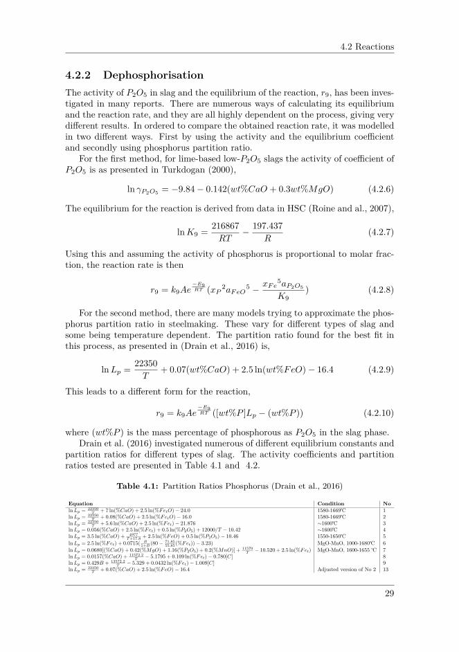
4.2.2 DephosphorisationThe activity of P2O5 in slag and the equilibrium of the reaction, r9, has been inves-tigated in many reports. There are numerous ways of calculating its equilibriumand the reaction rate, and they are all highly dependent on the process, giving verydifferent results. In ordered to compare the obtained reaction rate, it was modelledin two different ways. First by using the activity and the equilibrium coefficientand secondly using phosphorus partition ratio.
For the first method, for lime-based low-P2O5 slags the activity of coefficient ofP2O5 is as presented in Turkdogan (2000),
ln γP2O5 = −9.84− 0.142(wt%CaO + 0.3wt%MgO) (4.2.6)
The equilibrium for the reaction is derived from data in HSC (Roine and al., 2007),
lnK9 = 216867RT
− 197.437R
(4.2.7)
Using this and assuming the activity of phosphorus is proportional to molar frac-tion, the reaction rate is then
r9 = k9Ae−E9RT (xP 2aFeO
5 − xFe5aP2O5
K9) (4.2.8)
For the second method, there are many models trying to approximate the phos-phorus partition ratio in steelmaking. These vary for different types of slag andsome being temperature dependent. The partition ratio found for the best fit inthis process, as presented in (Drain et al., 2016) is,
lnLp = 22350T
+ 0.07(wt%CaO) + 2.5 ln(wt%FeO)− 16.4 (4.2.9)
This leads to a different form for the reaction,
r9 = k9Ae−E9RT ([wt%P ]Lp − (wt%P )) (4.2.10)
where (wt%P ) is the mass percentage of phosphorous as P2O5 in the slag phase.Drain et al. (2016) investigated numerous of different equilibrium constants and
partition ratios for different types of slag. The activity coefficients and partitionratios tested are presented in Table 4.1 and 4.2.
Table 4.1: Partition Ratios Phosphorus (Drain et al., 2016)
Equation Condition NolnLp = 22350
T + 7 ln(%CaO) + 2.5 ln(%FetO)− 24.0 1580-1669℃ 1lnLp = 22350
T + 0.08(%CaO) + 2.5 ln(%FetO)− 16.0 1580-1669℃ 2lnLp = 22350
T + 5.6 ln(%CaO) + 2.5 ln(%Fet)− 21.876 ∼1600℃ 3lnLp = 0.056(%CaO) + 2.5 ln(%Fet) + 0.5 ln(%P2O5) + 12000/T − 10.42 ∼1600℃ 4lnLp = 3.5 ln(%CaO) + 4977
T+17.8 + 2.5 ln(%FeO) + 0.5 ln(%P2O5)− 10.46 1550-1650℃ 5lnLp = 2.5 ln(%Fet) + 0.0715( B
1+B (80− 71.8555.85 (%Fet))− 3.23) MgO-MnO, 1000-1680℃ 6
lnLp = 0.0680[(%CaO) + 0.42(%MgO) + 1.16(%P2O5) + 0.2(%MnO)] + 11570T − 10.520 + 2.5 ln(%Fet) MgO-MnO, 1600-1655 ℃ 7
lnLp = 0.0157(%CaO) + 11572.2T − 5.1795 + 0.109 ln(%Fet)− 0.780[C] 8
lnLp = 0.429B + 13572.2T − 5.329 + 0.0432 ln(%Fet)− 1.009[C] 9
lnLp = 22350T + 0.07(%CaO) + 2.5 ln(%FeO)− 16.4 Adjusted version of No 2 13
29

Chapter 4. Modelling
Table 4.2: Activity Coefficients Phosphorus
Equation Reference Noln γP2O5 = 1.01(23NCaO + 17NMgO + 8NFeO − 26300
T + 11.2) (Turkdogan, 2000) 10ln γP2O5 = −12.6− 0.134((%CaO) + 0.33(%MgO)) (Turkdogan, 2000) 11ln γP2O5 = −1.12(22NCaO + 15NMgO + 13NMnO + 12NFeO − 2NSiO2)− 42000
T + 23.58 (Basu and Seetharaman, 2007) 12
4.2.3 Iron Oxide RateDuring blowing the operator may add pellets, which is typically used in blastfurnaces and contain 60%-75% iron. This is to adjust the chemical composition,adding more iron and oxygen to the bath. As iron oxide, FeO, is unstable at lowertemperature, these pellets contain mostly Fe2O3. When the pellets are melted intothe slag phase, it reacts with the iron in the bath, creating pure iron oxide, FeO.
r10 = k10Ae−E10
RT (xFe2O3xFe −aFeO
3
K10) (4.2.11)
where the equilibrium constant is,
lnK10 = −67595 + 84.267TRT
(4.2.12a)
4.2.4 Other Reaction RatesCentre Reactions
In the impact area of the oxygen jet, the oxygen enters the bath with supersonicvelocity. This rapidly reacts with the species in the bath, creating carbon monoxideand oxides to the slag.
The reactions between oxygen and other species are modelled with respect tothe likelihood of an oxygen molecule hitting an atom of another species. Thesereactions are modelled on the assumption that no reversible reactions occur.
α =5∑k=1
γkσkxi (4.2.13a)
rk = ηFO2
α
xiσk
(4.2.13b)
where γk and σk is the stoichiometry coefficients for the oxygen component and themetal component, respectively, in reaction k, where k = {1, 2, 3, 4, 5} for the reac-tions 4.2.1. FO2 [mol/s] is the utilised oxygen flow rate, η is the oxygen utilisationfactor and xi the molar fraction of the metal component, i, in the reaction.
Oxidation of Silicon
The activity of silicon dioxide is dependent on the concentration of the other speciesin the slag, as presented in the ternary in Figure 2.3. The reaction rate is modelledas,
r7 = k7Ae−E7RT (aSi(aFeO)2 − aSiO2(xFe)2
K7) (4.2.14)
30

4.3 Oxygen Jet
where (Ohta and Suito, 1998),
log aSiO2 = 0.036(wt%MgO) + 0.061(wt%Al2O3) + 0.123(wt%SiO2)
− 0.595B− 6.456
(4.2.15a)
log γ◦Si = −6100/T + 1.21 (4.2.15b)
lnK7 = 437846RT
− 82.544R
(4.2.15c)
Oxidation of Manganese
Assuming that the activity of manganese and iron in the metal is proportional tothe molar fraction, the reaction rate is
r8 = k8Ae−E8RT (xMnaFeO −
xFeaMnO
K8) (4.2.16)
where aMnO is dependent on the basicity and the equilibrium is,
K8 = (%MnO)(%FeO)[%Mn] (4.2.17a)
logK8 = 7452.0T
− 3.478 (4.2.17b)
Post-Combustion Rate
In this model it is assumed that there is full post-combustion, that means that allof the carbon monoxide reacts with oxygen to create carbon dioxide. Using thisassumption the reaction rate for post-combustion is,
r11 = r2 + r6 (4.2.18)
This assumption is also used later for calculating the amount of false air enteringthe waste gas hood.
4.3 Oxygen JetDeo and Boom (1993) presented different methods of calculating the penetrationdepth, the method used in this model is,
dH = Lh exp (−0.04147X2 + 1.3418X − 8.4297) (4.3.1a)
where
X = ln(M/L3h) (4.3.1b)
M = 1.421d2tp0[1− (pamb/pO)0.286] 1
2 (4.3.1c)
31

Chapter 4. Modelling
Lh is the lance height relative to the bath, dt is the throat diameter of the nozzle,pamb is the ambient pressure and pO is the oxygen pressure.
Using the penetration depth, the reaction constants are (Hammervold, 2010),
ki = ai + bidH (4.3.2)
where dH is the penetration depth found in equation 4.3.1 and ai and bi is param-eters for tuning. i is the reaction index, as listed in 4.2.1.
4.3.1 Emulsion and Metal-slag Interfacial AreaEmulsion
The emulsion height, or foam height, is an important process factor for the operatorto avoid slopping. Slopping is the event when the slag foam is forced through theconverters mouth. It is a frequent phenomenon in top-blown converters. Therehas been done some extensive work on predicting the foam height in the converter.A simple model was presented in (Sarkar et al., 2015b), but this showed too lowfoam height and was not dependent on the gas flow. Zhang and Fruehan (1995)presented a model including the gas flow, viscosity and surface tension of the slag.Defined as,
h = 115 µ1.2
D0.9b ρσ0.2 j (4.3.3)
where j is the superficial gas flow, Db is the metal droplet diameter, ρ is density ofslag, µ is the viscosity of slag and σ is the surface tension. µ, σ and Db is adaptedfrom Jung and Fruehan (2000).
Bramming (2010) did a thorough investigation in the predicting the foam height.He found that the vessel vibrations had good correlation with the foam height.Since neither vessel vibration or off-gas measurements (except temperature) areavailable, the emulsion height in this model is modelled as in equation 4.3.3.
Metal-slag Interfacial Area
For the reaction between the slag and bulk phase, the interfacial area is dependenton both the geometric area, but also the number of metal droplets in the slag phase.This can be modelled as (Subagyo et al., 2003)(Turkdogan, 2010),
A = Abulk,slag + xdropletVslagddroplet
(4.3.4)
xdroplet is the fraction of metal droplets in slag, and ddroplet is the diameter ofthe metal droplets. These values are set to fixed values, xdroplet = 0.05 andddroplet = 3mm.
In addition, it is expected that the interfacial area is also dependent on thebottom stirring. Higher stirring effect will lead to more oxides, FeO in particular,
32

4.4 Mass Transfer
circulate the bulk phase and react with the trace species in the metal. Hence,increasing the reaction rate. Including the metal droplets in slag, the area is,
A = Abulk,slag + xdropletVslagddroplet
+ xoxidewbτ
ρdoxide(4.3.5)
Where τ is a time constant for the residence time of oxides in the metal bath.
4.4 Mass TransferUsing the equation 2.4.3 in Section 2.4 and assuming the density is constant throughthe control volume the equation simplifies to
dm
dt= m = −
∫∫ρv>ndA (4.4.1)
Then the mass balance for each species in the control volume is
mi = wi,in − wi,out (4.4.2)
where i represents the species in the control volume and win and wout is the masstransfer in and out of control volume, respectively. Figure 4.3 illustrates the masstransfers between the bath control volumes.
Figure 4.3: Resulting mass transfer from agitation and stirring
The mass balance for the bulk control volume includes the scrap melting, stir-ring from centre and bottom and the reactions with the slag phase.
mFe = wFe,in − wFe,out +MFe(r6 + 2r7 + r8 + 5r9 − r10) + xFewmelt (4.4.3a)
mC = wC,in − wC,out −MCr6 + xCwmelt (4.4.3b)mSi = wSi,in − wSi,out −MSir7 + xSiwmelt (4.4.3c)
mMn = wMn,in − wMn,out −MMnr8 + xMnwmelt (4.4.3d)mP = wP,in − wP,out − 2MP r9 + xPwmelt (4.4.3e)
33
Chapter 4. Modelling
For the slag phase, the mass balance includes the dissolution of fluxes in additionto the reactions.
mFeO = MFeO(r1 − r6 − 2r7 − r8 − 5r9 + 3r10) + xFeOwdissolution (4.4.4a)
mSiO2 = MSiO2(r3 + r6) + xSiO2wdissolution (4.4.4b)mMnO = MMnO(r4 + r8) (4.4.4c)mP2O5 = MP2O5(r5 + r9) (4.4.4d)mCaO = xCaOwdissolution (4.4.4e)mMgO = xMgOwdissolution (4.4.4f)
mFe2O3 = MFe2O3(−r10) + xFe2O3wdissolution (4.4.4g)wdissolution is the dissolution rate of additive materials and xi is the molar fraction.
Only the centre reactions and the stirring affect the mass transfer for the centrecontrol volume. Hence, the mass transfer can be summarised as,
mi = wi,in − wi,out −Miσkrk (4.4.5)
where σk is the stoichiometry coefficients for the metal component in reaction rkfor k = 1, 2, 3, 4, 5. The molar masses used in the model are presented in Table 4.3
Table 4.3: Molar masses in [g/mol] for selected species (Roine and al., 2007)
Species Fe C Si Mn P FeO SiO2 MnO P2O5 CaO MgO Fe2O3Molar mass 55.85 12.01 28.09 54.94 30.97 71.85 60.08 70.94 141.94 56.08 40.30 159.69Gas species O2 CO CO2 N2 ArMolar mass 32 28.01 44.01 28.01 39.95
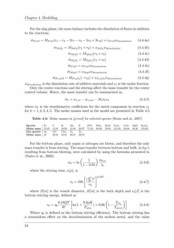
For the bottom phase, only argon or nitrogen are blown, and therefore the onlymass transfer is from stirring. The mass transfer between bottom and bulk, in kg/sresulting from bottom blowing, were calculated by using the formulas presented in(Naito et al., 2002).
wb = ln(
11− 0.95
)mtot
tb(4.4.6)
where the stirring time, tb[s], is
tb = 100[
(D2
H )2
eb
]0.337
(4.4.7)
where D[m] is the vessels diameter, H[m] is the bath depth and eb[J ] is thebottom stirring energy, defined as
eb = ηb6.18QTW
[ln(1 + 9.8ρH
Patm) + 0.06
(1− TO2
Tsteel
)](4.4.8)
Where ηb is defined as the bottom stirring efficiency. The bottom stirring hasa tremendous effect on the decarburisation of the molten metal, and the value
34

4.5 Dissolution of Additions and Scrap Melting
of this parameter is expected to vary in time due to wear on bottom tuyeres. Inreality, the converter has several tuyeres where each tuyere can be clogged or partlyclogged. As there is no data on this, the stirring efficiency parameter is expectedto reproduce same results.
4.5 Dissolution of Additions and Scrap MeltingTo achieve the desired composition and temperature of the steel bath, it is oftennecessary to add certain additions. These additions may have big influences on theslag behaviour or the molten bath behaviour. Adding scrap to the molten bathdoes not only decrease costs, but it also increases the content of iron and cools thebath. The addition of fluxes as lime and pellets gives the operator the possibilityto alter the kinetics and temperature of the slag.
Melting of scrap is a dissolution phenomenon where both heat transfer andmass transfer between solid and liquid phase takes place. Carbon governs themass transfer between the two phases if the carbon content of the liquid phaseis much higher than in the solid phase, the absorption of carbon from liquid tosolid decreases the melting temperature of solid phase (Li and Provatas, 2008). Inaddition, the added scrap, in general, has much lower temperature than the bath.Hence, there forms a solidified layer around the scrap. This layer and the additivesis then melted and diffused into the liquid phase. Both of these phenomena affectthe total melting time of the addition.
For the dissolution of solid oxides in the slag phase, it is dependent on the slagcomposition, temperature of the slag phase and the mixing between metal and slagphase (Dogan et al., 2009).
The melting and dissolution mechanism vary for the different types of additions.Here important factors are the melting temperature of the addition, grain size andsolubility of the additives. For simplification, the generation of a solid layer aroundthe addition material and the difference in carbon content is ignored. Hence themelting rate and dissolution rate can be simplified to these equations
dR
dt≈ khtc(T − Tm)ρ(∆hL + C(T − T0)) (4.5.1)
where ∆hL and khtc are the latent heat and heat transfer coefficient, respectively.Tm and T0 are the melting temperature and loading temperature of the addition.
The dissolution rate of lime is assumed to be dependent on the liquidus tem-perature of lime, while the dissolution rate of dolomite is expressed in terms of thesaturation of MgO,
wlime,dissolution = mslag
10 Klime(Tslag − Tliq) (4.5.2a)
wdolo,dissolution = mslag
10 Kdolo(MgOsat − xMgO) (4.5.2b)
where Ki is the activity coefficient, Tliq is the liquidus temperature and xMgO isthe molar fraction of MgO in slag.
35

Chapter 4. Modelling
The liquidus temperature of the slag is calculated using the equation presentedin (Seetharaman et al., 2014)
Tliq = 958+656.9xSiO2+1440.7xCaO+1091xMgO+761xMnO+522xFeO+794xFe2O3
(4.5.3)where Tliq is the liquidus temperature in Kelvin and xi is the weight fraction ofthe species. This has further been refined in order fit the phase diagram presentedin Figure 2.3 with the simulated process data during this work.
Tliq = 1131+565xSiO2+1110.7xCaO+1091xMgO+761xMnO+422xFeO+794xFe2O3
(4.5.4)With the slag composition ranging from 0% CaO to 70%CaO it is difficult to createone equation with good accuracy for all the phase fields. The equation has alsobeen averaged to fit the measured data given by SSAB.
Without knowing more about the additives with respect to their size and shapes,this is assumed to be a valid modelling of the rates. As the additives used in theprocess vary in shapes and size, it makes it hard in practice to take these factorsinto account.
4.6 Heat TransferThe majority of the heat transfers in the bath is due to radiation or conductionbefore the slag phase is created the bulk and centre control volume has a large sur-face area. During this, both the bulk and the centre loose heat to the surroundingsin the form of radiation, when the slag phase is formed the radiation from the bulkphase is practically zero. This is modelled by using Equation 2.6.2.
qrad = σRεSAi(T 4i − T 4
ref ) (4.6.1)
Where Ai is the surface area of the control volumes, the surface area for radiation iscalculated using the area of the converters mouth, such that the area of the centreis
Arad,centre = hbathhcentre
cmrAmouth (4.6.2)
Where cmr is the ratio between centre control volume mass and the total mass ofmetal. h is the height of the bath and centre. The slag area is found by taking theminimum of the cross-sectional area and slag area based on a minimum height of2 cm.
The heat transfer between the phases is due to conduction, and is calculatedby Equation 2.6.3.
For heat transfer with both convection and conduction, or through differentmaterials, one needs an averaged heat transfer coefficient. This can be calculatedas,
kave = 2k1k2
k1x1 + k2x2(4.6.3)
36

4.6 Heat Transfer
Where ki is the heat transfer coefficient or the thermal conductivity of the material,xi is the distance. For N transitions and N + 1 temperatures, the heat transfercan be generalised to
Q = T1 − TN+1∑Ni=1Ri
(4.6.4)
where
Ri ={
xi
kiA, conduction
1hiA
, convection(4.6.5)
4.6.1 Reaction HeatThe heat of reaction is the amount of heat needed to be added or withdrawn tokeep the products at the same temperature as the reactants. Assuming the pressurein the vessel is constant, this reaction heat can be calculated using enthalpy. Theheat of reaction is then either endothermic or exothermic, most of the net reactionsoccurring in a steel process are exothermic. When oxygen reacts with the speciesin the bath energy is released and the temperature of the bath increases. Figure 4.4presents the difference in energy between the reactants A and B to the product C.
Figure 4.4: Exothermic reaction
Note the increase in energy before the decrease, this comes from the heatingof reactants. Hence, the total heat of reaction can be calculating summing theheat added to the reactants and the difference in energy between the product andreactants, as formulated in (Deo and Boom, 1993).
∆H◦,reactT = ∆H◦,react298 + (H◦T2+H◦T1
)products − (H◦T2+H◦T1
)reactants (4.6.6)
Where ∆Ho,react298 is the heat of reaction when the products and reactants are in
their standard state at 298 K. By assuming that the reactions occur at the averagetemperature in their respective control volume, the heat of reactions is included inthe formulated energy balance.
37

Chapter 4. Modelling
4.6.2 Heating of Converter WallsIn order to make the simulation of the process continuous, temperature monitoringof the converter lining is added. During blowing heat transfers from the differentphases to the lining, hence the there is a difference from a batch with a cold con-verter to a batch with a warm converter. The lining of the converter consists ofdifferent materials. It is mainly divided into three different parts, working lining,safety lining and a steel cape. To make the temperature profile in the lining accu-rate, several temperatures are included in the lining. The first is at the surface ofthe working lining and will be at approximately the same temperature as the bath.The next is at 10%, and 30% in the working lining, 80% in the safety lining andthe last is at the steel cape. The temperature profile is presented in Figure 4.5.
Figure 4.5: Temperatures in the converters lining
The last two temperatures remain nearly constant through the batches, whilethe first three vary highly with the temperature of the bath and slag.
4.7 FumeThe exhaust system is divided into several sections. The first part is the lower partof the waste gas hood, placed directly above the mouth of the converter. Here thegas from the process together with some false air from the surroundings is suckedin by the exhaust system. The remaining oxygen from the bath reactions and theoxygen from the false air reacts with the carbon monoxide to create carbon dioxide,this is known as post-combustion. The gas is then cooled in the remaining wastegas hood before it gets further cooled in the exhaust system, after cooling the gasenters a scrubber for cleaning.In the steel refining process there is a limited amount of data during the blowingperiod, but by measuring the exhaust temperature and the cooling effect in theexhaust system, it is possible to withdraw information about the systems states.
38

4.7 Fume
From measuring the fume temperature in addition to the cooling effect, informa-tion about the reactions and temperature can be withdrawn and can indicate thecomposition of the bath.
4.7.1 Fume CompositionThe exhaust system is modelled in mol/s, and it is assumed that full combustiontakes place, as given from SSAB. In order to calculate the temperature changeand the composition of the gas in the exhaust, it is necessary to find the amountof false air that is sucked into the exhaust system. With the assumption of fullcombustion, this can be calculated by
Fi = Fi,in − Fi,out (4.7.1)
whereFi,in = Fi,wastegas + Fi,air (4.7.2)
An illustration of the energy and gas flow is presented in Figure 4.6.
Figure 4.6: Energy flow in waste gas hood
For each species the gas flow is
FCO,wastegas = r2 + r6 (4.7.3a)FO2,wastegas = (1− η)FO2,injection (4.7.3b)FCO2,wastegas = 0 (4.7.3c)FN2,wastegas = FN2,stirring (4.7.3d)FAr,wastegas = FAr,stirring (4.7.3e)
39

Chapter 4. Modelling
Fi,air is dependent on the needed oxygen for full combustion, η is the oxygenutilisation of the metal bath. The injection and stirring flows are all inputs to themodel. The flow out of the control volume, Fi,out, is dependent on how fast thefume flow is. Knowing the exhaust flow makes it possible to find the flow out of thevolume and hence the flow of fresh air. The fume flow consists of CO(g), CO2(g),O2(g), N2(g) and Ar(g).
As only CO(g), CO2(g) and O2(g) take part in the post combustion the molbalance of the waste gas hood becomes:
FCO = r2 + r6 (4.7.4a)
FO2 = 12r11 (4.7.4b)
FCO2 = −r11 (4.7.4c)FN2 = 0 (4.7.4d)FAr = 0 (4.7.4e)
4.7.2 Cooling Effect
The exhaust system is divided into three different control volumes, the hood abovethe converter where it is assumed that the post-combustion occurs, the upper partof the waste gas hood with cooling and the exhaust system with cooling.
Before the exhaust gas from the process enters the cleaning system, it is cooleddown by a parallel flow of water. In this u-shaped cooling stack, as illustratedin Figure 4.7, the cooling water first enters the upper part of the waste gas hoodbefore entering the cooling stack. The output flow is then measured in terms ofmass flow, temperature and the heat power generated.
40

4.7 Fume
Figure 4.7: Exhaust cooling system
In order to simplify the calculations of the cooling effect, logarithmic meantemperature difference is used instead of partial differential in the Cartesian coor-dinate system. The logarithmic mean temperature difference for a co-current flowis defined as,
TLMTD = (Th,in − Tc,in)− (Th,out − Tcout)ln (Th,in − Tc,in)− ln (Th,out − Tcout)
(4.7.5)
Where Th and Tc denote hot and cold side. Using LMTD, the heat from convectiveheat transfer can be written as,
Qc = hcATLMTD (4.7.6)
where hc is the heat transfer coefficient, and A is the surface area. The heat transfercoefficient depends on space, time, geometry, fluid properties and orientation of thesurface relative to the flow.
Since the fume temperature and cooling temperature did not correspond wellto the measurements in the previous model (Dyrdal, 2017), some adjustments aremade to slow down the system. The previous model was modelled with no materialbetween the warm fume and the cooling water. By adding a thin layer of metal,the cooling system is more accurate and slows down the temperature increase inboth the off gas and the cooling water. This is modelled as presented in Figure 4.8.
41

Chapter 4. Modelling
Figure 4.8: Heat from fume to cooling water
By assuming that the kinetic and potential energy of the water flow at theoutput is equal to the input, we can describe the temperature change in waterusing energy balance as,
T = m(h(Tin)− h(Tout)) +QcmCp
(4.7.7)
4.8 Energy balanceBy assuming that the kinetic and potential energy for the system is negligible anddensity is constant through the control volume, the energy balance becomes
d
dt(m(h(T ) + p
ρ)) +
∑ωi(hi(Ti)) = Q−Ws (4.8.1)
Index i being the species present and wi is the mass flow crossing the control volumesurface, defined positive outwards. Since no work is done on the system
d
dt(m(h(T ) + p
ρ)) +
∑ωi(hi(Ti)) = Q (4.8.2)
The fraction between pressure and density becomes relatively small compared tothe specific enthalpy, since the density of metal is large. Using the same values asin Section 2.5
p
ρ= 101325Pa
3500kg/m3 = 28.95kJ/kg
compared to the specific enthalpy 1023.15kJkg at 1500℃ of iron. Hence, the expres-sion becomes
d
dt(mh(T )) +
∑ωi(hi(Ti)) = Q (4.8.3)
42

4.8 Energy balance
By assuming the change in enthalpy is dominated by the change of temperature
d
dt(mh(T )) ≈ mh(T ) +m
∂H
∂T
dT
dt(4.8.4)
By differentiating the specific enthalpy with respect to temperature, yields thespecific heat capacity.
d
dTHi(T ) = Cp,i (4.8.5)
The energy balance then becomes∑mihi(T ) + T
∑miCp,i +
∑wi(hi(Ti)) = Q (4.8.6)
by re-arranging the energy balance, the temperature change is derived
T = Q+∑
(wi,inhi(Tin)− wi,outhi(T ))−∑mihi(T )∑
miCp,i(4.8.7)
4.8.1 Consistency CheckTo verify that the mass balance and energy balance are correctly implemented, aconsistency check is added to the model. The mass balance check for each speciesin the converter can be summarised as,
mi = mi + Mi
Mjxjwadditives + xiwscrap (4.8.8)
where i is the metal species and j is an oxide.An enthalpy check was created for both the converter and the off gas system. Thisis modelled for the converter as,
0 = Hin −Hout − (∆Hcentre + ∆Hbulk + ∆Hbottom + ∆Hslag) (4.8.9)
The energy check is modelled as,
0 = Et − E0 −∫ t
0Edt (4.8.10)
This also makes it possible to verify that the thermodynamic library and the datawritten into it is correct.
43

Chapter 4. Modelling
4.9 Results
The model results presented are simulated using SSAB’s process data. SSAB hasprovided data for many batches with inputs, measurements and initialisation. Thisfacilitated the model validation and made it possible to check whether the assump-tions made in the modelling were realistic. However, due to the harsh environmentof the BOF process, there is a lack of measurements during blowing, and the cor-rectness of the inputs and measurements are uncertain. Since the data provided bySSAB are confidential, no charge specification or input data is presented, neitherare the values for the parameters found. The time axis is defined as from 0 to100%, denoting start and end of blow respectively.
In this section, the results from the modelling and the validation against processdata is presented. Cybernetica’s model adjustment and simulation tool, Modelfit,enabled for simulation of the model. With Modelfit the user can easily change theinitial states and parameters, add their own inputs to the system or add datasetscontaining charge specification, measurements and inputs. The main parameterswere roughly tuned by using the parameter optimisation in Modelfit, trial anderror further adjusted the parameters for the reaction rates and oxygen utilisation.The results have been validated against 14 batches with different initialisation andadditions, only some of these batches included slag measurements. Results thathave not changed from the preliminary project thesis is included in Appendix A.
4.9.1 Validation
Bath and Slag Temperature
The converter, centre- and slag control volume’s temperature is presented in Fig-ure 4.9. These temperatures are highly dependent on the additions and theirmelting- or dissolution rates, in addition to the exothermic or endothermic heatfrom reactions.
44

4.9 Results
0 10 20 30 40 50 60 70 80 90 100
1200
1300
1400
1500
1600
1700
1800
1900
2000
2100
2200
2300
Figure 4.9: Converter, centre and slag temperature during a batch
Metal and Slag Composition
The composition of trace species in the metal and slag during the course of blowingis presented in Figure 4.10. Due to the equilibrium modelling of the slag reactionsthe content of these species are highly correlated. The species presented for metalare C, Si, Mn and P , for slag the species are FeO, SiO2, MnO, P2O5, CaO,MgO and Fe2O3.
0 20 40 60 80 100
0
0.1
0.2
0.3
0.4
0.5
0.6
0.7
0.8
0.9
1
0 20 40 60 80 100
0
10
20
30
40
50
60
70
80
90
100
Figure 4.10: Content of species and oxides in metal and slag during blowing
45

Chapter 4. Modelling
Slag Reactions
The slag reactions are presented in Figure 4.11. The reactions presented are r6, r7,r8, r9, r10 and r11. Since all of these reactions reacts with iron oxide, these are asexpected highly dependent on the iron oxide content in the slag.
0 10 20 30 40 50 60 70 80 90 100
-10
-5
0
5
10
15
20
25
30
35
40
Figure 4.11: Slag reactions
46

4.9 Results
Off Gas Results
The comparison of simulated- (Tfume) and measured (Tmeas) fume temperature to-gether with the correlation is presented in Figure 4.12. In Figure 4.13 the simulatedtemperature profile of waste gas hood and off gas cooling water is presented againstthe measurement. Here Tc,wgh is the waste gas hoods cooling water temperatureand Tc,fume is the off gas cooling water temperature.
0 20 40 60 80 100
100
200
300
400
500
600
700
800
900
1000
200 400 600 800 1000
100
200
300
400
500
600
700
800
900
1000
Figure 4.12: The simulated fume temperature against the measured temperature
0 20 40 60 80 100
80
90
100
110
120
130
0 20 40 60 80 100
80
90
100
110
120
130
Figure 4.13: Simulated versus measured fume temperature
47
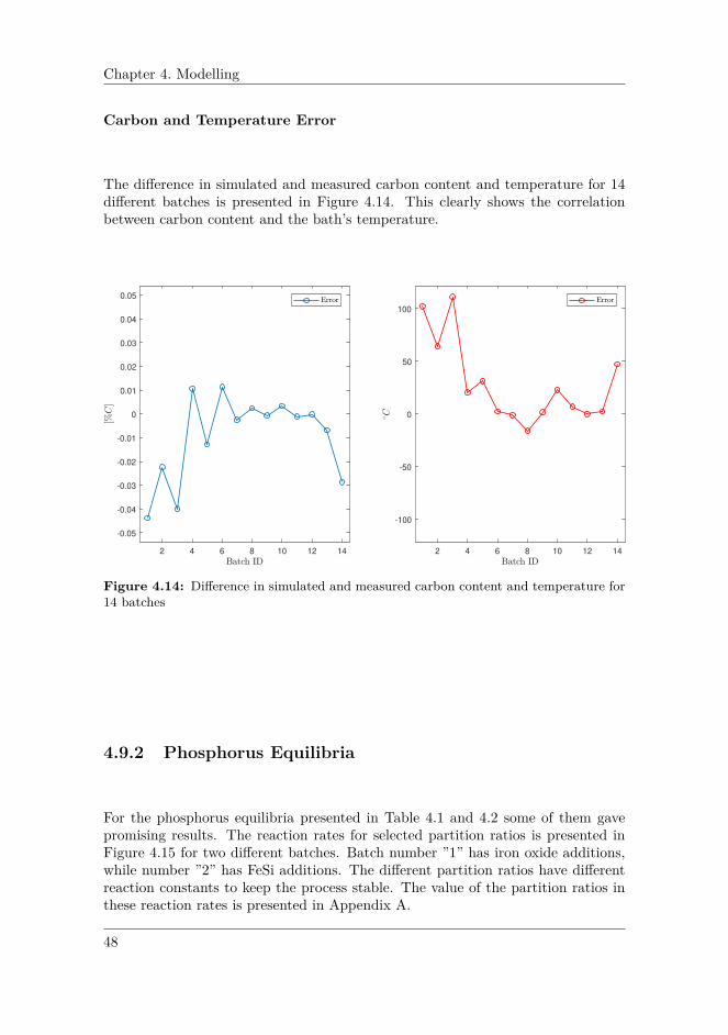
Chapter 4. Modelling
Carbon and Temperature Error
The difference in simulated and measured carbon content and temperature for 14different batches is presented in Figure 4.14. This clearly shows the correlationbetween carbon content and the bath’s temperature.
2 4 6 8 10 12 14
-0.05
-0.04
-0.03
-0.02
-0.01
0
0.01
0.02
0.03
0.04
0.05
2 4 6 8 10 12 14
-100
-50
0
50
100
Figure 4.14: Difference in simulated and measured carbon content and temperature for14 batches
4.9.2 Phosphorus Equilibria
For the phosphorus equilibria presented in Table 4.1 and 4.2 some of them gavepromising results. The reaction rates for selected partition ratios is presented inFigure 4.15 for two different batches. Batch number ”1” has iron oxide additions,while number ”2” has FeSi additions. The different partition ratios have differentreaction constants to keep the process stable. The value of the partition ratios inthese reaction rates is presented in Appendix A.
48

4.9 Results
0 20 40 60 80 100
0
1
2
3
4
5
6
7
8
No 1
0 20 40 60 80 100
0
0.5
1
1.5
2
2.5
3
3.5
No 2
0 20 40 60 80 100
0
0.5
1
1.5
2
No 3
0 20 40 60 80 100
-5
0
5
10
15
No 4
0 20 40 60 80 100
0
1
2
3
4
5
No 5
0 20 40 60 80 100
0
2
4
6
8
10
12
No 6
0 20 40 60 80 100
-2
0
2
4
6
8
10
12
No 7
0 20 40 60 80 100
-0.2
-0.1
0
0.1
0.2
0.3
0.4
No 8
0 20 40 60 80 100
-5
0
5
10
15
No 13
Figure 4.15: Reaction rates for selected phosphorus equilibria for two batches, Table 4.1
49

Chapter 4. Modelling
4.9.3 Emulsion Height
The emulsion height of a batch is presented in Figure 4.16. The y-axis representsthe height of the emulsion layer in meters.
0 10 20 30 40 50 60 70 80 90 100
0
0.2
0.4
0.6
0.8
1
1.2
Figure 4.16: Emulsion height during blowing
4.9.4 Lining Temperature
The different temperatures in the lining is presented in Figure 4.17. The tempera-tures presented are T0%, T10%, T30%, T80%, Tout as according to Figure 4.5.
50
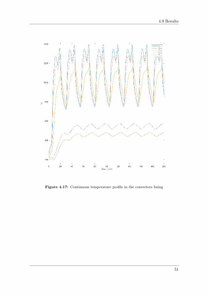
4.9 Results
Figure 4.17: Continuous temperature profile in the converters lining
51

Chapter 4. Modelling
4.10 Discussion4.10.1 Model ValidationThe goal of the modelling was to create a model which correlated well with themeasurements given by SSAB and the behaviour that is recommended in liter-ature and could further be used with an estimator and a controller. With theinfrequent and few available measurements in the BOF process, a well-correlatedmodel is beneficial in estimating the process’ states. There are different measuresto validate the model. The main focuses were the bath’s temperature, carbon-and phosphorus content. For measurements regarding the bath’s composition andtemperature, there are no measurements during the heat, the same applies to theslag phase. However, as mentioned earlier, the fume temperature and the coolingsystems temperatures are measured during the heat. By using these measurements,one could get a good indicator of whether the reaction kinetics (in particular theCO reactions) in the model is correlated with the real process.
A typical metal and slag content profile is presented in Turkdogan (2010),
Figure 4.18: BOF trace specie and slag profile, adapted from Turkdogan (2010)
Temperature Profiles
The end temperature of the bath correlated well with the measurements given bySSAB. Comparing the carbon content and the temperature against the measure-ments, the temperature of the bath is behaving as it should. Higher carbon contentthan measured yields a lower temperature than measured, and lower carbon con-tent yields a higher temperature. This is in line with the thermodynamics of the
52

4.10 Discussion
process, as the main producer of heat is the decarburisation.The bath’s temperature profile is naturally affected by the scrap melting. Whenthe bath’s temperature reaches the melting temperature of scrap, the temperatureincrease nearly stops until most of the scrap is dissolved into the molten metalbefore it increases. Comparing the bath’s temperature profile with literature andmodels presented by Kruskopf and Visuri (2017), it should, however, keep a morelinear profile. This may be solved by changing the melting kinetics of scrap to amore advanced model, taking into account an increasing temperature of the scrap.As it is modelled now, Equation 4.5.1, the temperature of the scrap remains con-stant at ambient temperature. This causes the scrap to draw more energy in thestart before it heats up and dissolves into the metal.
Metal and Slag Composition
For the metal composition, the silicon content does not decrease as rapidly as sug-gested in Turkdogan (2010). This is a consequence of the low level of iron oxide inthe slag. However, the profile fits well with other models presented in literature,such as Kruskopf and Visuri (2017) and Sarkar et al. (2015a). Here the siliconcontent decreases quickly the first 20% before remaining about constant towards80% of the blowing time.
Figure 4.14 presented the carbon and temperature error for 14 different batches.These results show high deviations from the measured results for the three firstbatches and the last batch. Discussing these batches with SSAB, it showed thatfor the first batch, the bottom stirring was almost non-existing, requiring a muchlonger blowing time. For the other batches, the source of the error is unknown. Tohave full faith in the measurements, more information about the process and themeasurements from the heat is required.
The iron oxide content in the slag is lower than what is expected, but theend-point content fits well with the few measurements given on the slag content.Comparing the profiles of CaO, SiO2 and FeO with Figure 4.18, Kruskopf andVisuri (2017) and Sarkar et al. (2015a). The profiles match well with Figure 4.18and the results presented in Sarkar et al. (2015a), with a slowly decreasing SiO2content due to the decreasing amount of Si in the metal, low FeO content in the slaguntil the carbon content approaches its equilibrium and high CaO content from theadded lime. However, it does not match well with the results presented in Kruskopfand Visuri (2017) and the model compared against in the report. It is hard to saywhich one is more accurate for this process without having measurements of theslag content during blowing. The slag weight after the heat would also be a goodindicator of which is correct.
Reaction Kinetics
The centre reaction rates are modelled the same way as in the preliminary reportand are presented in Appendix A.
53

Chapter 4. Modelling
The reaction kinetics between iron oxide and carbon is modelled with the equilib-rium depending on the partial pressure of CO-bubbles, activity of iron oxide andthe equilibrium constant. In Figure 4.19 the equilibrium, and measured data forBOP and Q-BOP are presented as in Turkdogan (2010) together with the simu-lated results from the model. The low iron oxide content in the model’s slag isevident here as well, to the match the measured carbon content, the equilibrium isadjusted down. However, at higher iron oxide content, it correlates well with themeasured Q-BOP results.
0 0.1 0.2 0.3 0.4 0.5 0.6
0
2
4
6
8
10
12
14
16
Figure 4.19: Correlation between iron oxide and carbon content in literature (left) andmodel (right), literature graph adapted from Turkdogan (2010)
In the previous model, the oxygen utilisation was set to full utilisation, usingall of the oxygen blown into the furnace. This led naturally to a higher iron oxidecontent in the slag during the heat, but it also led to that the endpoint contentof iron oxide being higher than measured. A possible way of solving this is tohave a varying degree of oxygen utilisation during the heat. Decreasing the oxygenutilisation with decreasing carbon content may cause the iron oxide content in theslag to keep a higher level during oxygen blowing and match the measurements.
Fume and Cooling System
The fume’s temperature profile matches the measurement to some degree, as pre-sented in Figure 4.12. In order to match the increasing fume and cooling watertemperature, a metal layer between the fume and cooling water was added. Thisacts as a time constant for both of the temperature profiles as this layer takessome time before reaching the fumes temperature. Even though this improved theresults, it still lacks some of the characteristics in the measurements. It is hard topinpoint the reason for this delay in temperature increase for the fume. The wastegas volume flow in the off-gas channel is not measured, nor is the power delivered tothe fan. The flow in the model is set to a constant value, but it can be expected thatthe volume flow in the channel decreases when the fume’s temperature increases.The post-combustion is modelled to occur instantly with full combustion, and thatthe reaction receives all the necessary oxygen from either the process or as false airfrom the surroundings. This may be a too strong assumption, and modelling the
54

4.10 Discussion
reaction with chemical equilibrium may improve the results. By doing this, it mayslow down the reaction until it receives enough oxygen for full combustion.
The lack of increase in fume temperature is evident in the cooling waters tem-perature as this remains at a constant level during blowing. For the waste gashood’s cooling water, the temperature does not reach the same level as the mea-surements. There are some uncertainties in the design of the cooling system, asthere is a lack of technical drawings of the system such as cooling pipe radii andthe layout of these pipes.
4.10.2 Phosphorus EquilibriaThere has been done much work in trying to find an equilibrium for the phospho-rus during the production of steel. However, these equilibria vary highly and oftenonly applies for a certain type of slag and other processing conditions. For thephosphorus partition ratios and activity coefficients presented in Table 4.1 and 4.2,only a few gave promising results that were numerical stable during simulation.It is expected that the phosphorus reaction is heavily dependent on the CaO andFeO content, and the dephosphorisation decrease with increasing temperature dueto its endothermic nature of the reaction. The reaction rate should, therefore, below during mid-heat as the slag temperature is high and the FeO content is low,while it is expected to be high at the start and end of the heat. The differentequilibria were tested with two different heats that have different additions duringthe heat. None of the activity coefficients gave promising reaction rates results. Bymodelling the reaction rate with activities of the species, the rate is very vulnerableto changes in the iron oxide content as this is raised to the power of five. Hence,small changes in the iron oxide content have large effects on the dephosphorisationrate. For the partition ratios reaction rates presented in Figure 4.15, many of themgave promising results.
For the partition ratio number three and five, the corresponding reaction ratekept a relatively high value throughout the heat, not corresponding to the expectedkinetics and resulted in too low phosphorus content, compared to measurements.For partition ratio number eight, the reaction rate was nearly linearly increasingfrom a negative rate until about 80% of the heat. Here, the reaction rate becamestiff and numerically unstable. This relates to the relatively high dependency ontotal iron in the slag phase compared to the other partition ratios, in combinationwith low CaO dependency and low constant term. Partition rate number four,seven and the adjusted version of number two, number thirteen, all correspondedwell with the kinetics given in literature and measurements given by SSAB. Thephosphorus content decreases at the start of blowing, before increasing again andremaining constant until towards the end of the heat, where it decreases to below≈ 0.01%. Number four and thirteen gave very similar results and correspondedwell with measurements. However, number thirteen was chosen as the partitionratio used for this model since it corresponded better with measurements and issimpler than number four.
55

Chapter 4. Modelling
4.10.3 Emulsion HeightThe emulsion height in the model was modelled according to Equation 4.3.3. Thevalues used for the viscosity and surface tension of the slag were averages fromseveral different slag measurements given in Jung and Fruehan (2000). SSAB doesnot have any measurements of the emulsion height during heats. Hence the heightis compared to what is expected from literature such as Bramming (2010) andwhat can be expected with regards to the converters geometry. The resultingemulsion height has a reasonable value and does not indicate slopping. The profilealso matches what could be expected, as the lance height in the start is higher,resulting in larger iron oxide production and higher decarburisation rate.
4.10.4 Lining TemperatureIt is expected that the temperature outermost in the lining remain about constantthrough and in between heats, while the temperature in the working lining varywith the temperature of the bath. This matches well with the results presentedin Figure 4.17. The temperature for T80% and Tout remains nearly constant. Thetemperature profile of T0% and T10% is highly correlated with the bath’s temper-ature profile, which is as expected as this takes up a large amount of the volumeand has a larger heat transfer coefficient than the slag and gas phase. Due to thelarge volume of the T30%, it has a slower temperature profile and does not reach aslow temperature as the two innermost temperature profiles.
56

4.11 Conclusions
4.11 ConclusionsDue to the harsh and extreme environment of the BOF process, there is a lack ofinstrumentation. For the plant studied, the measurements available for heat are theend-point steel composition, possible slag analysis and the off-gas systems temper-atures. With the lack of measurements, the BOF process has been operated basedon experience and the operator’s knowledge about the previous batches accuracy.However, with a model based control system, a state estimator can use the modelto predict the process behaviour and update the model with the available measure-ments. In this chapter, a model has been further developed and compared againstprocess data from a steel plant. The main foci of the modelling were to createa complete model which could replicate the process behaviour and correctly pre-dict the steel composition and temperature. Comparing the model results with thegiven data, the model produced good results for most of the batches simulated. Forsome batches, the model deviated from the measurements. Further investigationshowed that this might be a result of the loss of bottom stirring in the converter.For the slag composition, the model results correlated well with the batches withslag analysis. However, the iron oxide content in the slag during oxygen blowingwas lower than what is expected. The fume temperature profile does not matchthe measured temperature profile, and without more information about the off-gasduct and its cooling system, it is hard to identify the problem.
Several phosphorus equilibria were investigated with the model. Two partitionratios were found to give the best fit by comparing the results from this with theprocess data and the suggested profile in literature. Partition ratio number 4 and13. The model was augmented with continuous monitoring of the temperature inthe converters lining. The lining’s temperature matched the expectations, withhigher variations closer to the metal bath. In addition, a model for the emulsionheight was implemented. The emulsion height model produced reasonable emulsionheights that did not correspond to slopping.
57

Chapter 4. Modelling
58

Chapter 5Predictive Monitoring
This chapter describes Cybernetica’s tools for simulation, estimation and control,and how the estimator and controller has been designed. The results from theestimation and control cases is presented, followed by a discussion and conclusions.
5.1 Setup5.1.1 Utilised SoftwareCybernetica has several tools to support the development of the model, estimatorand controller.
Modelfit
For model validation and offline estimation, Cybernetica’s Modelfit is used. Mod-elfit is used for estimating the parameters assumed to be constant, which param-eters should be estimated online and designing the online estimator part of Cenitapplications. Modelfit supports multiple data sets from different operating condi-tions, allowing to find the best parameter fit for all conditions considered.
Cenit
Cenit is a powerful and versatile software suite for nonlinear model predictive con-trol. Since it uses nonlinear mechanistic models, it is a better and more robustalternative to technologies that rely on linear models. The Cenit application con-sists of a user interface and a kernel. The interface displays the measurements,estimates and control inputs. The kernel communicates with the user interface,and handles the data transfer with the OPC server, database and the processmodel. The Cenit application is built on top of Cenit SDK. Cenit SDK is a col-lection of calculation models used in estimation and nonlinear model predictivecontrol. Several interfaces can be implemented, depending on which calculation
59

Chapter 5. Predictive Monitoring
modules that shall be used. It is possible to implement different models for eachinterface, i.e. the controller has a simpler model than the simulator. Cenit SDKconsists of interfaces for simulation, Kalman filtering, moving horizon estimation,NMPC, Modelfit and async data.The model is implemented in the model template in Cenit. In this template allthe necessary calculations and the differential equations presented in the previoussection is implemented. In addition, it contains different solvers for ODE.
RealSim
Cybernetica RealSim is a plant replacement simulator used for testing of the Cenitmodules. RealSim and Cenit communicates through OPC in order to replicate adistributed control system. As mentioned, the simulator may use a different modelthan the model implemented in the controller. In this project the simulator andcontroller use the same model. The noise added to the system is implemented inRealSim’s simulator interface.
5.1.2 Implementation
Through Cybernetica’s tools, the model has been validated and adjusted, and theestimator and controller have been configured. Using Modelfit, the parametersin the model have been adjusted using an optimisation tool in addition to trialand error. After this, the results from model fitting has been validated againstthe measurements given by SSAB. These datasets are the same as used duringthe preliminary report. During simulation, RealSim and Cenit are used. RealSimsimulates the data and sends the data to the local OPC server where Cenit canread the measurements, inputs and outputs. After the estimator and controlleris finished with the calculation, Cenit sends the new control inputs to the OPCserver, and RealSim can apply this to the model. During the simulation, Cenitlogs the selected data to a local SQL database. This is illustrated in Figure 5.1.
60

5.1 Setup
Figure 5.1: Communication between interfaces, model and software
The model presented in the previous section is implemented on the followingform in Cenit SDK. The solver used for integration for this model is the 2nd orderRunge-Kutta.
xk = f(xk−1, uk−1, θ, vk−1)yk = g(xk, uk−1, θ) + wk
zk = h(xk, θ, uk−1)(5.1.1)
wherexk = Model states at time tkθ = Model parameters
uk−1 = Process inputs from [tk−1, tk]yk = Measurement at time tk
vk−1 = White process noisewk = White measurement noisezk = Output variable (CV)
(5.1.2)
5.1.3 Heat RecipeIn order to have full faith in the measurements and no uncertainties in weights orgas injected, a heat recipe was created to simulate data. This also enables to usethe waste gas measurements to indicate the possibilities with these measurements.The recipe was created by the author, and is inspired by the pattern given inliterature, such as (Turkdogan, 2010), and the data given by SSAB. In order tokeep the data from SSAB confidential, the heat recipe has been altered.
The inputs to the system (MV) is presented in Table 5.1.
61

Chapter 5. Predictive Monitoring
Table 5.1: Model inputs
Index MV Description Unit1 QO2 Oxygen blown by lance [Nm3/min]2 Lh Lance height [m]3-8 Qi Injection gases in bottom [Nm3/s]9-15 wi Addition rate [kg/s]16 Tc Cooling water inlet temperature [K]17 tO2 Oxygen blowing time [s]
The injection gases are bottom injection of different gases, only Ar and N2 areused. Addition of different fluxes such as pellets, lime and dolomite and scrap areavailable. Cooling water is the water inlet temperature in to the cooling system inthe off-gas system. tO2 is the blowing time for the batch.
The oxygen flow rate and lance height recipe is presented in Figure 5.2.
0 t
0
50
100
150
200
250
300
350
0
1
2
3
4
5
6
7
8
9
10
11
Figure 5.2: Oxygen and lance height profile
The injection of argon and nitrogen is presented in Figure 5.3.
62

5.1 Setup
Figure 5.3: Injection of Argon and Nitrogen
The amount of hot metal added to the converter with its content and the amountof additive materials is presented in Table 5.2.
Table 5.2: Batch details
InitializationHot metal 104000 kgSlag 0%C 4.5%Si 0.6%Mn 0.18%P 0.061%S 0.009Scrap 26000 kgTemperature 1350℃Total additionsLime 6500 kgPellets 3000 kg
63

Chapter 5. Predictive Monitoring
5.2 MHEIn this section, the configuration of the moving horizon estimator is presented. Thestate-space model is presented in Equation 5.1.1. The measurement and outputmodel is the same. For the estimator, the system and its parameters are subjectto additive white noise,
xk+1 = f(xk, uk, θk) + vs,k
θk+1 = θk + vp,k(5.2.1)
The state vector is augmented with the parameters to facilitate for parameterestimation. vs,k and vp,k is the noise added to the states and parameters. Thesystem is subject to the constraints
xlow ≤ x ≤ xhighθlow ≤ θ ≤ θhighulow ≤ u ≤ uhighylow ≤ y ≤ yhighvmin ≤ v ≤ vmax
(5.2.2)
The optimisation problem for the MHE then becomes,
ΦT = minx0,...,xT
Γ(x0) +T−1∑k=0
v>k V−1k vk +
T∑k=0
w>kW−1k wk (5.2.3)
whereΓ(x0) = (x0 − x0)>Π−1
0 (x0 − x0) (5.2.4)Π0 is the state covariance matrix, initialised by σx0 and σθ0 ,
Π0 = E{[x0, θ0]>[x0, θ0]} = diag([σx0 , σθ0 ])diag([σx0 , σθ0 ]) (5.2.5)
Where σx0 and σθ0 are tuning parameters for the estimator. For T > N , 0 denotesT −N .The process and measurement noise covariance matrices are defined as,
Vk = E{v>v} = diag(σv)diag(σv) (5.2.6)
Wk = E{w>w} = diag(σw)diag(σw) (5.2.7)In this project, no specific states are estimated. Instead, the parameter estimateshandle the possible deviation in measurements and estimates. By doing this, theenergy and mass balance are still valid. The parameters to be estimated in thisproject are the oxygen utilisation (η) and/or the bottom stirring efficiency (ηb).These parameters are expected to be varying between batches. The oxygen util-isation is assumed to be varying with a Gaussian distribution, while the bottomstirring efficiency is assumed to have a degrading efficiency before maintenance,where the efficiency then increases again. This assumption is based on the data
64

5.2 MHE
given by SSAB on the carbon-oxygen factor (4.2.1) for a series of batches, wherethere is a similar trend. The entries in the covariance matrix with their correspond-ing constraints is then,
Table 5.3: Non-zero MHE tuning parameters
Variable Type σ [low, high]η Parameter 0.01 [0.8, 1]ηb Parameter 0.05 [0.1, 1]
The process noise is assumed to be additive in the estimator. The noise addedto the states are listed in Table 5.4. The number of blocks are the number ofparameters used to parameterize the process noise in the horizon.
Table 5.4: MHE process noise tuning parameters
Disturbance σ Blocksvη 1.3e-5 No. of batchesvηb
1.8e-5 2
Here vη is the process noise on the oxygen utilisation parameter and vηbis the
process noise on the bottom stirring efficiency.
For the process the actual measurements are listed in Table 5.5. These mea-surements are measured after the batch is finished, hence the only measurementupdate for the MHE is after finished blowing and the system has stabilized. Thismakes the estimation problem harder as the estimator has no measurement updatesduring blowing. For the process considered the only measurements during blowingare the waste gas and cooling system measurement. Since there are some uncer-tainties with these measurements and the model’s results are not correspondingwell with the process, these measurements are not used. The uncertainty relatedto the measurements, σ, is roughly set to 1% of the final value.
65

Chapter 5. Predictive Monitoring
Table 5.5: Mean and variance of measurements
Measurement σ UnitSteelSteel mass 1000 kgC 0.0001 %Si 0.00001 %Mn 0.001 %P 0.0001 %S 0.00001 %Steel temp 10 ◦CSlagFeO 0.1 %SiO2 0.1 %MnO 0.01 %P2O5 0.01 %CaO 0.1 %MgO 0.01 %Fe2O3 0.01 %FumeFume temp 30 ◦C
5.3 NMPCThe general NMPC optimisation problem with the model given in Equation 5.1.1takes the form,
min∆U
J(Z,∆U) = min∆U
0.5(Z − Zref )>Q(Z − Zref ) + 0.5∆U>S∆U
+ r>1 ε+ 0.5ε>diag(r2)ε (5.3.1)
where
Z = [zT , zT+1, . . . , zT+N ] (5.3.2a)∆U = [∆uT ,∆uT+1, . . . ,∆uT+N ] (5.3.2b)
Z is the predicted output in the prediction horizon and Zref is the reference tra-jectory. ∆U is the optimal input trajectory for the control horizon and ε is themaximal constraint violation of each z variable. The matrices Q and S are thenormalized output and input weights and r1 and r2 are the linear and quadraticconstraint violation weights.
Objective Function
The main control objectives are to achieve steel temperature and carbon contentwithin the specification even with changing process factors such as oxygen utilisa-
66

5.3 NMPC
tion and bottom stirring efficiency. For this, the CV to be controlled is the carboncontent for the entire metal bath, and with a given recipe, this can be achievedby optimising the oxygen blowing time. Therefore the objective function can bewritten as,
J(Z,∆U) =NP∑0
0.5(%C − %Csp)2q +NC∑0
0.5∆t2O2s + r>1 ε + 0.5ε>diag(r2)ε
(5.3.3)
where NP and NC is the prediction- and control horizon. %Csp is the carboncontent set-point and tO2 is the oxygen blowing time. In addition to definingthe optimisation problem, we need to define how often the optimisation problemshould be solved. The sampling time of the controller should be fast enough toincorporate the system’s behaviour. Therefore, the sampling time should be muchshorter than the time constant of the CV we want to control. One should also keepin mind the computation time necessary to finish the optimisation problem. Thecomputational load is dependent on the free optimisation variables, the prediction-and control horizon and the parameters used to parametrise the horizon. The dy-namics of the carbon content in the metal is quite slow. Therefore the samplinginterval for the MPC can be extended. For this project, the sampling interval is 10s.
Since the control objective is focusing on the endpoint value and not the tra-jectory, it is practical to choose the prediction horizon long enough to predict theendpoint carbon content and only weight the last sample.For the control horizon, it is also favourable to have a long horizon so that the pro-cess is controlled with respect to the endpoint specification. The controller is onlyoptimising the blowing time, which should ideally keep a constant value throughoutthe batch, hence it is weighted on the current sample. For the other control inputs,they are read from the recipe, therefore these values are only weighted on the lastsample of the horizon. This is summarized in Table 5.6.
Table 5.6: Control and prediction horizon
Horizon Weighted samples LengthControl 149 24 min 50 sControl(tO2) 0 24 min 50 sPrediction 150 25 min
Configuration of MV and CV
The weights, nominal value and target of the MV and CV are listed in Table 5.7.With two variables in the objective function, it is fairly straightforward to set theweights. Since the target is to achieve the desired carbon content in the steel,the deviations from the set-point is set much higher than the cost of changingblowing oxygen. This, in addition to the nominal value of the MV, ensures thatthe controller quickly finds the optimum.
67

Chapter 5. Predictive Monitoring
Table 5.7: Configuration of MV and CV
Parameter tO2 z[%C]weight 1e-6 1e3nominal value max(tO2 , 10 min) -target - 0.035%
The constraints on the input and output are listed in Table 5.8.
Table 5.8: Constraints on MV and CV
Constraint tO2 z[%C]min 1 min 0max 30 min 100
5.4 Simulations
The tests are simulated with a fixed recipe set by the author for each heat, as pre-sented in Section 5.1.2. The main goal for the estimator is to predict the correctoxygen utilisation η, and the correct bottom stirring efficiency ηb, and hence pre-dict the correct amount of carbon content in the metal. For the controller, the aimis to calculate the optimal blowing time for the heat with the estimated parametersto achieve the desired carbon content. The estimator results are simulated usingModelfit, while the optimal control cases are simulated using RealSim and Cenit,as described in Section 5.1.2.
The variation of oxygen utilisation and bottom stirring efficiency is presentedin Figure 5.4. The degrading efficiency in the bottom stirring should replicate theprocess’ behaviour when the bottom tuyeres start getting clogged before havingmaintenance, and the efficiency improves.
68

5.4 Simulations
0 50 100 150 200 250 300 350 400 450 500
0
0.1
0.2
0.3
0.4
0.5
0.6
0.7
0.8
0.9
1
Figure 5.4: Variation of oxygen utilisation and bottom stirring efficiency
In order to demonstrate the capabilities and limitations with the estimator andlimited amount of measurements, the estimator is tested with different disturbancesand measurements. These cases are listed in Table 5.9. The optimal control casesare based on the estimator cases and are listed in Table 5.10.
Table 5.9: Estimation and control cases with configuration of MHE
Case Disturbance Estimator setupση vη Blocks σηb
vηbBlocks Horizon
1 Intial offset in η 0.01 0 1 0 0 0 3 batches2 White noise on η 0.01 1.3e-5 3 0 0 0 3 batches3 Decreasing and increasing ηb 0 0 0 0.2 0 1 3 batches4 Varying η and ηb 0.01 0 1 0.05 0 1 1 batch5 Varying η and ηb 0.01 1.3e-5 3 0.05 1.8e-4 2 3 batches6 Varying η and ηb with slag meas. 0.01 1.3e-5 3 0.05 1.8e-4 2 3 batches7 Varying η and ηb with fume meas. 0.01 1.3e-5 3 0.05 1.8e-4 2 3 batches8 Varying η and ηb with sub-lance meas. 0.01 1.2e-5 3 0.05 1.5e-4 2 3 batches9 50% reduction in carbon reaction constant 0.01 0 1 0 0 0 3 batches10 Initial error in metal content with fume meas. 0.05 1.0e-5 3 0 0 0 3 batches
Table 5.10: Optimal control cases
Case Disturbance Measurement Estimator setup Controller setup11 Decreasing and increasing ηb End point steel Case 3 zsp[%C]12 Varying η and ηb End point steel and slag Case 6 zsp[%C]13 Varying η and ηb End point steel and slag with cont. fume Case 7 zsp[%C]14 Varying ηb and sine varying η End point steel and slag Case 6 zsp[%C]15 50% reduction in carbon reaction constant End point steel and slag Case 9 zsp[%C]16 Initial error in metal content and varying ηb End point steel and slag with cont. fume Case 7 zsp[%C]17 Initial error in metal content End point steel and slag with cont. fume Case 10 zsp[%C]
69

Chapter 5. Predictive Monitoring
5.5 Results
In this section, the results from the estimation and optimal control cases in Table 5.9and 5.10 are presented.
5.5.1 Estimation Results
Estimation of η
The initial configuration of the estimator was done in Modelfit with the cases listedin Table 5.9. The estimator performance for an initial offset in oxygen utilisationis presented in Figure 5.5.
0 20 40 60 80
0.87
0.88
0.89
0.9
0.91
0.92
0.93
Figure 5.5: Estimation with an initial offset in η, case 1
Figure 5.6 presents the estimation results of applying white noise on the oxygenutilisation parameter, η. Furthermore, it presents the estimated carbon content ofthe metal against the real value.
70

5.5 Results
0 100 200 300 400 500
0.88
0.9
0.92
Figure 5.6: Estimation with varying η, case 2
Estimating η and ηb
Figure 5.7 and 5.8 presents the online estimation of the oxygen utilisation η andthe bottom stirring efficiency, ηb, for the estimation cases 4, 5 and 6. In addition,it presents the estimated carbon content of the metal and the estimation error ofcarbon.
71

Chapter 5. Predictive Monitoring
0 100 200 300 400 500
0.88
0.9
0.92
0 100 200 300 400 500
0.2
0.4
0.6
0.8
1
0 100 200 300 400 500
-0.1
0
0.1
Figure 5.7: Estimation with varying η and ηb, case 4
0 100 200 300 400 500
0.88
0.9
0.92
0 100 200 300 400 500
0.2
0.4
0.6
0.8
0 100 200 300 400 500
-0.1
0
0.1
Figure 5.8: Estimation with varying η and ηb, case 5 and 6
72

5.5 Results
Lance Measurement
Figure 5.9 presents the results from adding a sub-lance measurement of the steelfour minutes before the planned end of the heat. The same disturbances are appliedto the bottom stirring and oxygen utilisation as the earlier results without sub-lancemeasurement.
0 100 200 300 400
0.86
0.88
0.9
0.92
0.94
0 100 200 300 400
0.2
0.4
0.6
0.8
1
0 100 200 300 400
-0.1
-0.05
0
0.05
0.1
Figure 5.9: Estimation results for varying ηb and η with lance measurements, case 8
73

Chapter 5. Predictive Monitoring
5.5.2 Control ResultsPerfect model without disturbances
The control results using a perfect model without any disturbances is presented inFigure 5.10. The temperature profile of the metal bath is presented along with thefume temperature, carbon content and iron oxide content.
0 50 100 150 200 250
1400
1500
1600
1700
0 50 100 150 200 250
200
400
600
800
Figure 5.10: Estimation and control results with perfect model
74

5.5 Results
Reduction in decarburisation constant
Figure 5.11 presents the results from having an initial error in the offline estimateof the decarburisation constant.
0 10 20 30 40 50 60 70
0.89
0.9
0.91
0.92
0.93
0.94
Figure 5.11: Estimation and control results for 50% reduction of decarburisation con-stant, case 15
75

Chapter 5. Predictive Monitoring
Varying ηb
Figure 5.12 presents the results from estimating the bottom stirring efficiency withonly end-point measurements. It presents the online estimation of the bottomstirring efficiency and how the controller deviates from the set-point. The realvalues presented in the graphs are the values used by the simulator.
0 50 100 150 200 250 300 350 400 450 500
0.2
0.4
0.6
0.8
1
Figure 5.12: Estimation and control results with varying ηb, case 11
76

5.5 Results
Varying η and ηb
The control results for endpoint with slag measurement and without estimationis presented in Figure 5.13. The error plot presents the simulated carbon contentdeviation from the set-point, with and without estimation.
0 50 100 150 200 250
0.8
0.85
0.9
0.95
1
0 50 100 150 200 250
0
0.2
0.4
0.6
0.8
1
1 2 3 4 5 6 7 8 9 10
-0.05
0
0.05
0.1
0.15
Figure 5.13: Estimation and control results for varying η and ηb with slag measurements,12
77

Chapter 5. Predictive Monitoring
The results from adding the fume measurements is presented in Figure 5.14
0 50 100 150 200 250
0.8
0.85
0.9
0.95
1
0 50 100 150 200 250
0.2
0.4
0.6
0.8
1
1 2 3 4 5 6 7 8 9 10
-0.02
0
0.02
0.04
0.06
0.08
0.1
0.12
Figure 5.14: Control results for varying η and ηb with fume measurements, case 13
78

5.5 Results
Varying ηb and sine varying η
The results from applying a sinusoidal disturbance to the oxygen utilisation anda varying bottom stirring efficiency are presented against no estimation in Fig-ure 5.15.
0 100 200 300 400 500
0.8
0.85
0.9
0.95
1
0 100 200 300 400 500
0.4
0.6
0.8
1
1 2 3 4 5 6 7 8 9 1011121314151617181920
-0.02
0
0.02
0.04
0.06
Figure 5.15: Control results with and without estimation for varying ηb and sine varyingη, case 14
Initialization Error
It is expected that there are some uncertainties in the initial specification of themetal. The results from applying white noise to the initialisation of the batch arepresented in Figure 5.16 and 5.17. These are simulated with continuous fumetemperature measurement. Case 16 has also a disturbance on the bottom stirringefficiency. Towards the end of the simulation, the initial error is so significant thatboth oxygen utilisation and bottom stirring reaches its upper limit.
79

Chapter 5. Predictive Monitoring
0 100 200 300 400
0.8
0.85
0.9
0.95
1
0 100 200 300 400
0.3
0.4
0.5
0.6
0.7
0.8
0.9
1
1 2 3 4 5 6 7 8 9 10 11 12 13 14 15 16 17
-1
-0.8
-0.6
-0.4
-0.2
0
0.2
0.4
1 2 3 4 5 6 7 8 9 10 11 12 13 14 15 16 17
-0.03
-0.02
-0.01
0
0.01
0.02
0.03
Figure 5.16: Control results for varying ηb and initialization error, case 16
80

5.5 Results
0 50 100 150 200 250
0.8
0.85
0.9
0.95
1
1 2 3 4 5 6 7 8 9 10
-0.1
0
0.1
0.2
0.3
0.4
1 2 3 4 5 6 7 8 9 10
-10
-8
-6
-4
-2
0
2
410
-4
Figure 5.17: Control results for initialization error, case 17
81

Chapter 5. Predictive Monitoring
5.6 Discussion
5.6.1 Estimator Results
The availability of measurements is a crucial factor in the performance of the es-timator. This is evident in the cases tested with different measurements available.For the cases with end-point steel measurements, the estimator does not updatethe parameter estimates during the heat, and hence the end result is only affectedby the measurements given earlier in the horizon. To verify the configuration ofthe estimator, a simple case with an offset in the oxygen utilisation parameter ispresented in Figure 5.5. The estimator quickly finds the correct parameter valuewhen the measurements become available. If these parameters are affected by inde-pendent noise, the estimator is not capable of predicting the next parameter valuewithout any measurements during the heat, resulting in too low or high carboncontent. This is presented in Figure 5.6. The cases with disturbances on bothoxygen utilisation and bottom stirring is presented in Figure 5.7 and 5.8. In case4, the estimator had an estimation horizon of one batch. This resulted in that theoxygen utilisation was only updated with the previous oxygen utilisation, leadingto large errors in the carbon predictions. In case 5, the estimator had an estima-tion horizon of three batches. The estimator has issues with estimating both ηand ηb for large variations in η, this resulted in large variations in the estimatesof the bottom stirring. For the bottom stirring efficiency, it is expected that thisparameter is slowly decreasing before maintenance. This slow decrease facilitates abetter parameter estimate as presented in Figure 5.12. The results from having adisturbance trend in the horizon is also presented in Figure 5.15. Here the oxygenutilisation, η, has a varying value following a sinusoidal curve with the bottomstirring varying as previously. This results in a considerable better estimate thanfor independent disturbances, with the estimator being able to predict a reasonablevalue for both η and ηb.
Figure 5.8 presents the different estimation results for different measurements.If only measuring the end-point steel content, the estimator has an observabilityproblem when estimating both η and ηb. Decreasing the bottom stirring efficiencyleads to lower carbon content in the metal, but it also leads to a higher contentof iron oxide in the slag due to the low carbon concentration in centre and bulk.By adding a measurement of the slag at the end of the heat, in addition to thesteel, the estimator should be able to estimate a better value for these two pa-rameters, and in particular, the bottom stirring. The slag measurements improvethe estimate of the parameters, but the estimator still has issues with the largechanges in the oxygen utilisation, leading to a rather poor estimate of the carboncontent. The fume modelling results did not lead to a good representation of theprocess’ behaviour, but the results using the fume measurements are included topresent the possible improvements, the results are presented in Figure 5.14. Byusing the fume measurements, the parameter estimate has improved. The estima-tor produces reasonable parameter estimates, and the estimated fume temperaturematches the measured. With reasonable parameter estimates, the estimated car-
82

5.6 Discussion
bon content correlates well with the measured end-point content. This holds trueexcept for when the bottom stirring efficiency changes from decreasing to increas-ing efficiency, leading to considerable deviations.
There is a significant improvement by adding a sub-lance measurement fourminutes before the planned end of the heat, as presented in Figure 5.9. By addingthis, the estimator handles the significant changes in oxygen utilisation and thebottom stirring efficiency. For batch number 17, if the changes in oxygen utilisa-tion are too significant, the sub-lance measurement comes too late, resulting in aconsiderable deviation from the real value.
5.6.2 Control ResultsThe controller was configured to calculate the optimal blowing time of oxygen withrespect to the carbon content in the metal. As there was no economic perspectiveor any strict constraints on this optimisation problem, the carbon content weightswere set high enough to quickly find the optimal time without considering the cost.For a perfect internal model with no external disturbances, the controller satisfiedthe end-point carbon content specification perfectly, as presented in Figure 5.10.
Without Estimator Feedback
Since there doesn’t exist any direct measurement from the converters environment,disabling the estimator is the same as removing the feedback to the controller.Hence, the controller finds the optimal blowing time based on an erroneous model.As presented in Figure 5.14, this results in poor controller performance.
With Estimator Feedback
The ability to estimate an oxygen utilisation to compensate for errors in otherparameters was investigated in case 15. As visible in Figure 5.11, the estimatorquickly finds the oxygen utilisation to compensate for the offset and the controllerachieves the desired end-point content. The control results from using bottom stir-ring efficiency estimation are presented in Figure 5.12. The parameter estimationis, as discussed earlier, quite good. The controller achieves the desired carbon con-tent in the steel except for when the bottom stirring efficiency changes from havinga decreasing efficiency to increasing. This is as expected, as the estimator does notreceive any information about maintenance.
For the cases with significant variations in the oxygen utilisation, the estimatordoes not produce an accurate estimate of the parameters, as presented in Fig-ure 5.13. With only end-point measurements the estimator does not have enoughinformation to produce reasonable estimates of the oxygen utilisation for the batch.This is evident in the carbon error plot, in some cases the results from not having
83

Chapter 5. Predictive Monitoring
state estimation is equally good, or even better, as with state estimation. A prob-lem that may arise when estimating significant changes in the oxygen utilisation isthe stiffness of the slag reactions. During heat, the iron oxide content in the slag islower than expected. Increasing the oxygen utilisation has, therefore, a significanteffect on the slag reactions, as the iron oxide content in the slag increases. It is alsoworth noting that for the cases where the resulting carbon content is approximately0.02%, the equilibrium is reached, and the carbon content does not decrease anymore, Figure 4.2. As discussed in the previous section, the results of adding moremeasurements are much better. The estimator produces a reasonable parameterestimate, resulting in a more accurate carbon content at turn-down, as presentedin Figure 5.14.
For the initialisation errors, the simulation was subject to initial error in thetotal steel weight and the content of the trace species. In addition, the case pre-sented in Figure 5.16 has varying bottom stirring efficiency. The estimation andcontrol results were investigated with respect to the carbon content. The estimatorproblem was to estimate the oxygen utilisation and bottom stirring efficiency tocompensate for the initialisation error and the varying bottom stirring efficiency.The results showed varying precision regarding correcting for the initialisation er-ror, with the resulting end-point carbon content error shifting from negative 0.02%to almost 0.03%. The last simulated batches had a very low true carbon content,resulting in full oxygen utilisation and bottom stirring efficiency. This full utilisa-tion should alarm the operator, as it is very unlikely to have this high utilisation.It is also not expected that the error of the initialisation is in the magnitude of1% carbon. For initialisation errors of less magnitude and without bottom stirringdisturbance, the estimator was able to track the fume temperature perfectly, aspresented in Figure 5.17. However, it should be noted that by only estimating theparameter value for oxygen utilisation, the converter’s temperature will not matchthe real value. Although the estimator matches the fume temperature and achievesthe desired end-point content, it does not compensate for the difference in carboncontent in the metal, which has a significant effect on the converter’s temperature.
Computational Load
For the cases with large variations on the oxygen utilisation and the bottom stirringefficiency, a more complex noise model was needed to achieve reasonable estimatesand to increase the robustness of the estimator. With the process model developedin this work, this came at a high cost concerning computational load. For case 12with a sampling time of 10 seconds, the estimator and controller used on average30 seconds per sample. If this should be applied to a real plant, the design of thecontrol system and the model need to be considered. Creating a simpler model thatcan have a higher integration step and still replicates the process behaviour wouldlead to a considerable reduction in computation load. If neither a simpler modelor a simpler noise modelling is possible, the control systems need to be designedto handle the high computational demand.
84

5.7 Conclusions
5.7 ConclusionsIn this chapter, the use of a moving horizon estimator and model predictive controlon a BOF converter has been studied. The estimator performance was tested byestimating the parameter values for the oxygen utilisation and bottom stirring effi-ciency, in the presence of disturbances on parameter values and initialisation valuesby using a noise corrupted simulator. With an initial offset in oxygen utilisation,the estimator quickly found the correct value. For the cases with slow variationsin parameter values, the estimator produced good estimates and in combinationwith the controller achieved the desired carbon content in the steel. Independentdisturbances with high variations led to inconsistent parameter estimates and de-viations from the set-point. By adding more measurements for the estimator, theperformance improved. The conclusions from this are that for high variations be-tween batches the estimator does not have enough information from the end-pointmeasurements to provide good estimates for the next batch.
Today, the BOF process is in general controlled by static charge calculationsand the operator’s experience. In this work, the use of an NMPC to find the opti-mal oxygen blowing time is studied. The controller uses a predefined heat recipe forthe oxygen blowing rate, lance height and additions. The controller was found toperform well for the cases with accurate estimates. For the cases with significantvariations, the poor estimates led to considerable deviations from the set-point.For initialisation errors, the estimator is able to compensate for initialisation er-rors in the carbon content by estimating the oxygen utilisation. However, by onlyestimating the parameter values, the estimated converter temperature differs fromthe real value.
The computational load of using an MHE approach for estimation is consider-able. For the most complex cases, the control system is far slower than the samplingrate.
85

Chapter 5. Predictive Monitoring
86

Chapter 6Overall Conclusions and FurtherWork
6.1 Conclusions
In this thesis, a comprehensive model of the BOF process is further developed froma preliminary project. This model includes modelling of the off-gas system, continu-ous lining temperature and emulsion height, in addition to reaction kinetics betweenoxygen, metal and slag. The model has been validated against measurements givenby SSAB, Raahe. Furthermore, the implementation of moving horizon estimatorand nonlinear model predictive control is investigated. With the harsh and extremeenvironment of the BOF process, there are few measurements available. The fumetemperature is continuously measured, and the steel and slag content is measuredafter the batch is finished. By using a moving horizon approach to estimate theprocess’ state, the estimator can utilise the delayed measurements of metal- andslag analysis. Combining the estimator with an NMPC, the operator can achievea more efficient and accurate production.
The primary foci of the modelling were to develop a model which correlatedwith the measurements given by SSAB and proposed process behaviour in litera-ture. In addition, different phosphorus equilibria were evaluated, continuous liningtemperature and a model for the emulsion height were implemented. The modelresults matched well with the measurements given by SSAB in terms of steel andslag content at the end of the blow. For some batches, the model deviated from themeasurements. Further investigation showed that this could be a consequence ofthe loss of bottom stirring in the converter. The iron oxide content during oxygenblowing is considerably lower than expected, and the fume temperature profile doesnot match well with the measured temperature profile. Without more measure-ments during the process, it is hard to identify the possible problems.
87

Chapter 6. Overall Conclusions and Further Work
For the phosphorus equilibria investigated, two partition ratios were found to givethe best fit. Partition ratio number 4 and 13 correlated well with the process dataand characteristics proposed in literature. The lining’s temperature and the heightof the emulsion layer matched well with the expectations.
The estimator performance was tested by using a noise corrupted process simu-lator. The goal of the estimator was to predict the correct parameter values in thepresence of disturbances on parameter values and initialisation. For slow variationsin parameter values the estimator was able to produce reasonable estimates, andin combination with the controller achieved the desired carbon content in the steel.With independent disturbances with high variations, the estimator produced incon-sistent parameter values and substantial deviations from the set-point. By addingmore measurements for the estimator, the performance improved. The conclusionsfrom this are that for high variations from batch to batch, the estimator does nothave enough information from the end-point measurements to provide reasonableestimates for the next batch.The controller was configured to find the optimal oxygen blowing time and used apre-defined heat recipe for blowing rate, lance height and additions. The controllerperformed well for the cases with slow variations. For large variations, the poorestimates led to significant deviations from the set-point. With initialisation errorsthe estimator is able to estimate the parameter values to compensate for the dif-ference in initial carbon content, and the controller achieves the desired end-pointcontent.For the more complex test cases, the computational load was considerable, and thecomputation time was far slower than the sampling rate.
6.2 Further WorkThe model’s behaviour deviates from the measurements and expected behaviourin terms of the off-gas temperature and slag composition. To increase the valid-ity of the model, the model should be further tested against batches with moremeasurements. Running test heats at the plant with measurements during oxygenblowing by using a sub-lance would provide much-needed information about theslag and metal composition during the heat. This would also indicate whetherthe assumptions in the modelling of reaction rates and the equilibriums are accu-rate. By adding simple instrumentation in the process such as measurements ofthe fume flow or the power delivered to the fan would facilitate better validationof the off-gas modelling. Improving the accuracy of the waste gas measurementswould provide the estimator with more measurements, and improving the accuracyof the estimates.
The online estimation should be tested against real process data to study theend-point accuracy for batches with real disturbances. In addition, by furtherdeveloping the NMPC with additions of additives and scrap, the controller canimprove the accuracy regarding both carbon content and metal temperature.
88

6.2 Further Work
For implementation in a real process, the computation time needs to be de-creased. To reduce the computational load, the complexity of the model should berevised.
89

Chapter 6. Overall Conclusions and Further Work
90

Bibliography
Basu, S. and Seetharaman, S. (2007), ‘Studies on Dephosphorisation During Steel-making’, Materials Science and Engineering Ph.D.
Bramming, M. (2010), Avoiding Slopping in Top-Blown BOS Vessels.
Deo, B. and Boom, R. (1993), Fundamentals of steelmaking metallurgy, PrenticeHall International.
Dogan, N., Brooks, G. A. and Rhamdhani, M. A. (2009), ‘Kinetics of Flux Disso-lution in Oxygen Steelmaking’, ISIJ INternation 49(10), 1474–1482.
Dogan, N., Brooks, G. A. and Rhamdhani, M. A. (2011a), ‘Comprehensive Modelof Oxygen Steelmaking Part 1: Model Development and Validation’, ISIJ Inter-national 51(7), 1086–1092.
Dogan, N., Brooks, G. A. and Rhamdhani, M. A. (2011b), ‘Comprehensive Modelof Oxygen Steelmaking Part 2: Application of Bloated Droplet Theory for De-carburization in Emulsion Zone’, ISIJ International 51(7), 1093–1101.
Dogan, N., Brooks, G. A. and Rhamdhani, M. A. (2011c), ‘Comprehensive Modelof Oxygen Steelmaking Part 3 : Decarburization in Impact Zone’, ISIJ Interna-tional 51(7), 1102–1109.
Drain, P., Monaghan, B. J., Zhang, G., Longbottom, R. and Murgas, I. (2016),Development of a new phosphorus partition relation for Australian steelmakers,Technical report, Melbourne.
Dyrdal, B. M. (2017), Mathematical Modelling and Simulation of Basic OxygenFurnace, Technical report, NTNU.
Egeland, O. and Gravdahl, J. T. (2002), Modeling and Simulation for AutomaticControl, Marine Cybernetics.
Foss, B. and Heirung, T. A. N. (2016), Merging Optimization and Control.
91

Hammervold, A. (2010), Mathematical modeling of the Linz-Donawitz converter,Technical report, NTNU.
Hammervold, A. (2011), Model based estimation and control of a BOS converter(MSc thesis).
Han, M., Li, Y. and Cao, Z. (2014), ‘Hybrid intelligent control of BOF oxygenvolume and coolant addition’, Neurocomputing 123, 415–423.
Han, M. and Liu, C. (2014), ‘Endpoint prediction model for basic oxygen furnacesteel-making based on membrane algorithm evolving extreme learning machine’,Applied Soft Computing 19, 430–437.
Johansen, T. A. (2011), Introduction to Nonlinear Model Predictive Control andMoving Horizon Estimation, in ‘Selected Topics on Constrained and NonlinearControl’, chapter 5, pp. 187–233.
Jung, S. M. and Fruehan, R. J. (2000), ‘Foaming characteristics of BOF slags’,ISIJ International 40(4), 348–355.
Kruskopf, A. and Visuri, V.-V. (2017), ‘A Gibbs Energy Minimization Approachfor Modeling of Chemical Reactions in a Basic Oxygen Furnace’, Metallurgicaland Materials Transactions B 48(6), 3281–3300.
Li, J. and Provatas, N. (2008), ‘Kinetics of scrap melting in liquid steel: Multipiecescrap melting’, Metallurgical and Materials Transactions B: Process Metallurgyand Materials Processing Science .
Mazumdar, D. and Evans, J. W. (2010), Modeling of steelmaking processes, CRCPress.
Naito, K., Kitamura, S. and Ogawa, Y. (2002), ‘Effects of BOF top blowing andbottom stirring conditions on suppressing excessive oxidation’, Ironmaking &Steelmaking 29(3), 208–213.
Nocedal, J. and Wright, S. J. (2006), Numerical optimization, Springer.
Ohta, H. and Suito, H. (1998), ‘Activities of SiO2 and Al2O3 and activity coef-ficients of FetO and MnO in CaO-SiO2-Al2O3-MgO slags’, Metallurgical andMaterials Transactions B 29(1), 119–129.
Qin, S. J. and Badgwell, T. A. (2003), ‘An overview of industrial model predictivecontrol technology’, Control Engineering Practice 11(7), 733–764.
Rao, C. V., Rawlings, J. B. and Lee, J. H. (2001), ‘Constrained linear state esti-mation—a moving horizon approach’, Automatica 37(10), 1619–1628.
Rao, C. V., Rawlings, J. B. and Mayne, D. Q. (2003), ‘Constrained state estima-tion for nonlinear discrete-time systems: Stability and moving horizon approxi-mations’, IEEE Transactions on Automatic Control 48(2), 246–258.
92

Rawlings, J. B. and Mayne, D. Q. (2009), Model predictive control : theory anddesign, Nob Hill Pub.
Roine, A. and al., E. (2007), ‘HSC Chemistry’.
Sarkar, R., Gupta, P., Basu, S. and Ballal, N. B. (2015a), ‘Dynamic Modelingof LD Converter Steelmaking: Reaction Modeling Using Gibbs’ Free EnergyMinimization’, Metallurgical and Materials Transactions B 46(2), 961–976.
Sarkar, R., Gupta, P., Basu, S. and Ballal, N. B. (2015b), ‘Dynamic Modelingof LD Converter Steelmaking: Reaction Modeling Using Gibbs’ Free EnergyMinimization’, Metallurgical and Materials Transactions B 46(2), 961–976.
Seetharaman, S., McLean, A., Guthrie, R. I. L. and Sridhar, S. (2014), Treatise onprocess metallurgy, Elsevier.
Shamsuddin, M. (2016), Physical Chemistry of Metallurgical Processes, John Wiley& Sons, Inc, Hoboken, NJ.
Subagyo, Brooks, G. a., Coley, K. S. and Irons, G. a. (2003), ‘Generation ofDroplets in Slag-Metal Emulsions through Top Gas Blowing’, ISIJ International43(7), 983–989.
Turkdogan, E. (2000), ‘Assessment of P2O5 Activity Coefficients in Molten Slags’,ISIJ International 40(10), 964–70.
Turkdogan, E. T. (2010), Fundamentals of steelmaking, Institute of Materials(GreatBritain).
World Steel Organisation (n.d.), ‘About steel’.URL: https://www.worldsteel.org/media-centre/about-steel.html
Zhang, Y. and Fruehan, R. J. (1995), ‘Effect of carbonaceous particles on slagfoaming’, Metallurgical and Materials Transactions B 26(4), 813–819.
93

94

Appendix AModel Results
This appendix contains the model results that are not presented in Section 4.9.Figure A.1 presents the center reaction rates. Figure A.2 and A.3 presents thereaction rates for the different phosphorus equilibria presented in Table 4.1 and 4.2,and the partition ratios for the reaction rates presented in Section 4.9.2.
0 10 20 30 40 50 60 70 80 90 100
0
1
2
3
4
5
6
7
8
9
10
Figure A.1: Centre reaction rates
95

0 50 100
0
2
4
6
8
No 1
0 50 100
0
0.5
1
1.5
2
No 2
0 50 100
0
0.5
1
1.5
2
2.5
No 3
0 50 100
-5
0
5
10
15
No 4
0 50 100
0
1
2
3
4
No 5
0 50 100
0
2
4
6
8
10
No 6
0 50 100
-2
0
2
4
6
8
10
12
No 7
0 50 100
-0.2
-0.1
0
0.1
0.2
0.3
No 8
0 50 100
-0.2
0
0.2
0.4
0.6
0.8
1
No 9
0 50 100
-0.5
0
0.5
1
1.5
No 10
0 50 100
-0.7
-0.6
-0.5
-0.4
-0.3
-0.2
-0.1
0
No 11
0 50 100
-0.7
-0.6
-0.5
-0.4
-0.3
-0.2
-0.1
0
No 12
Figure A.2: Reaction rates for the different equilibriums, Table 4.1 and 4.2
96

0 20 40 60 80 100
101
No 1
0 20 40 60 80 100
0
0.5
1
1.5
2
No 2
0 20 40 60 80 100
101
No 3
0 20 40 60 80 100
0
20
40
60
80
100
No 4
0 20 40 60 80 100
0
20
40
60
80
100
No 5
0 20 40 60 80 100
0
20
40
60
80
100
No 6
0 20 40 60 80 100
0
20
40
60
80
100
No 7
0 20 40 60 80 100
0.5
1
1.5
2
No 8
0 20 40 60 80 100
0
20
40
60
80
100
No 13
Figure A.3: Selected partition ratios for two batches
97