predictive marine mammal modeling for queen charlotte ......predictive marine mammal modeling for...
TRANSCRIPT

Predictive Marine Mammal Modeling for Queen Charlotte Basin, British Columbia
Technical Report
Benjamin Best Patrick Halpin Marine Geospatial Ecology Lab Nicholas School of the Environment Duke University Marine Lab

Page 3 of 120
TABLE OF CONTENTS Foreword...................................................................................................................................................................2 List of Figures...........................................................................................................................................................5 List of Tables ..........................................................................................................................................................10
Introduction to the Project .......................................................................................................................................11 Survey Design.........................................................................................................................................................12 Species Observed and Conservation Status ............................................................................................................14 Abundance Estimation............................................................................................................................................19
TIER A. ESTIMATING ABUNDANCE .......................................................................... 21
Product 1. Using Conventional Distance Sampling ................................................................................................21 Methods ..................................................................................................................................................................21 Results ....................................................................................................................................................................22 Discussion...............................................................................................................................................................32
Product 2. Using Density Surface Models and Identifying Hotspots ....................................................................36 Methods ..................................................................................................................................................................36 Results ....................................................................................................................................................................40 Abundance Estimates..............................................................................................................................................42 Discussion...............................................................................................................................................................46
TIER B. COMPOSITE RISK MAP AND VESSEL ROUTING ....................................... 47
Introduction ...............................................................................................................................................................47
Methods ......................................................................................................................................................................48 Product 3. Composite Risk Map .............................................................................................................................48 Product 4. Vessel Routing.......................................................................................................................................49
Results.........................................................................................................................................................................50
Discussion ...................................................................................................................................................................55
REFERENCES.............................................................................................................. 56
APPENDIX 1. BRITISH COLUMBIA NAUTICAL CHARTS ......................................... 61
APPENDIX 2. MAPS OF OBSERVATIONS ................................................................. 68
Harbour porpoise ......................................................................................................................................................68
Dall’s porpoise ...........................................................................................................................................................69
Pacific white-sided dolphin .......................................................................................................................................70
Humpback whale .......................................................................................................................................................71
Fin whale ....................................................................................................................................................................72

Page 4 of 120
Killer whale ................................................................................................................................................................73
Minke whale ...............................................................................................................................................................74
Harbour seal, haul-out ..............................................................................................................................................75
Harbour seal, in-water ..............................................................................................................................................76
Stellar sea lion, haul-out............................................................................................................................................77
Steller sea lion, in-water............................................................................................................................................78
Elephant seal ..............................................................................................................................................................79
APPENDIX 3. MAPS OF ENVIRONMENTAL COVARIATES ...................................... 80
Depth...........................................................................................................................................................................80
Slope............................................................................................................................................................................81
Distance to Coast .......................................................................................................................................................82
Dynamic Variables: SST, Chl...................................................................................................................................83
APPENDIX 4. DENSITY SURFACE MODEL OUTPUTS ............................................. 84
Harbour Porpoise ......................................................................................................................................................84
Dall’s porpoise ...........................................................................................................................................................87
Pacific white-sided dolphin .......................................................................................................................................90
Humpback whale .......................................................................................................................................................93
Fin whale ....................................................................................................................................................................97
Killer whale ..............................................................................................................................................................100
Minke whale .............................................................................................................................................................103
Harbour seal, haul-out ............................................................................................................................................106
Harbour seal, in-water ............................................................................................................................................109
Stellar sea lion, haul-out..........................................................................................................................................112
Steller sea lion, in-water..........................................................................................................................................115
Elephant seal ............................................................................................................................................................118

Page 5 of 120
List of Figures Figure 1. Stratum ID and on-effort transects, including transit legs between design-based
transects, for all years, corresponding to Queen Charlotte Basin (1), Straits of Georgia and Juan de Fuca (2), Johnstone Strait (3), and mainland inlets (4). ................................ 13
Figure 2. Observations by species from all surveys. .................................................................... 15
Figure 3. Detection functions for conventional distance sampling (CDS) analysis. .................... 23
Figure 5. Abundance estimate comparisons between Williams & Thomas (2007) from the 2004-2005 surveys with the updated 2004-2008 survey data pooled across all strata and seasons. Note that with more data (eg 2004-2008), the confidence intervals consistently shrink. Species abbreviations are for harbour porpoise (HP), Dall's porpoise (DP), Pacific white-sided dolphin (PW), killer whale (KW), humpback whale (HW), common minke whale (MW), fin whale (FW), harbour seal (HS), Steller sea lion (SSL) and elephant seal (ES). Further abbreviations for pinnipeds denote haul-out (out), in-water (in) and total combined (tot)................................................................................................................... 33
Figure 6. Abundance with 95% confidence intervals over surveyed years and seasons in Stratum 1, including the average of all seasons. Summer averages are included for seasonal comparison with 2007 fall and spring. No significant differences were found across seasons or years per species.............................................................................................. 35
Figure 8. Average detection probabilities for density surface modeling (DSM) using the Multiple Covariate Distance Sampling (mcds) engine with the covariate size where possible, otherwise using Conventional Distance Sampling (cds) without a covariate. The detection function uses either a half-normal(“hn”) or hazard rate (“hr”) key function.................... 41
Figure 9. Comparison of abundance estimates for the entire region between conventional distance sampling from 2004 to 2005 (Williams and Thomas, 2007), conventional with the additional survey years to 2008, and density surface modeling, with 95% CI error bars.................................................................................................................................... 45
Figure 10. On the left, polygons of important areas for gray, humpback, and sperm whales derived from expert opinion in the PNCIMA Atlas (Draft 2009). On the right, proposed tanker vessel route for servicing the forthcoming Kitimat oil and gas projects (EnviroEmerg Consulting Services 2008). ....................................................................... 48
Figure 11. Weighting by BC conservation status for fin whale (FW), Steller sea lion (SSL), harbour porpoise (HP), humpback whale (HW), killer whale (KW), Elephant seal (ES), minke whale (MW), Dall’s porpoise (DP), Pacific white-sided dolphin, and harbour seal (HS)................................................................................................................................... 49
Figure 12. Conservation-weighted composite map of all marine mammal z-scored densities. ... 51
Figure 13. Conservation-weighted composite map of only large whales (killer, humpback, fin and minke) z-scored densities. .......................................................................................... 52

Page 6 of 120
Figure 14. Proposed, linear (Euclidean), and least-cost routes for Kitimat. The least-cost route uses the conservation weighted cost surface from Figure 11 pictured here. ................... 53
Figure 15. Existing, Euclidean and least-cost routes for cruise ships. The least-cost route uses a cost surface which is the sum of the conservation risk surface and a surface of distance from existing routes scaled to the equivalent range. The least cost-path is chosen which thus avoids biological hotspots while being equally attracted to existing routes. ............ 54
Figure 16. Nautical chart overview of B.C. .................................................................................. 61
Figure 17. Nautical chart for North Coast of B.C......................................................................... 62
Figure 18. Nautical chart for South Coast of B.C......................................................................... 63
Figure 19. Nautical chart for Large Scale North B.C. .................................................................. 64
Figure 20. Nautical chart for Large Scale North Vancouver Island. ............................................ 65
Figure 21. Nautical chart for Large Scale South Vancouver Island. ............................................ 66
Figure 22. Nautical chart for the Queen Charlotte Islands. .......................................................... 67
Figure 23. Observations of harbour porpoise by group size for all surveys (2004-2008), after truncating perpendicular distance (w) to within 600m. .................................................. 68
Figure 24. Observations of Dall’s porpoise by group size for all surveys (2004-2008), after truncating perpendicular distance (w) to within 700m. .................................................... 69
Figure 25. Observations of Pacific white-sided dolphin by group size for all surveys (2004-2008), after truncating perpendicular distance (w) to within 1200m................................ 70
Figure 26. Observations of humpback whale by group size for all surveys (2004-2008), after truncating perpendicular distance (w) to within 2300m. .................................................. 71
Figure 27. Observations of fin whale by group size for all surveys (2004-2008), after truncating perpendicular distance (w) to within 3900m..................................................................... 72
Figure 28. Observations of killer whale by group size for all surveys (2004-2008), after truncating perpendicular distance (w) to within 1300m. .................................................. 73
Figure 29. Observations of minke whale by group size for all surveys (2004-2008), after truncating perpendicular distance (w) to within 400m. .................................................... 74
Figure 30. Observations of harbour seal, haul-out, by group size for all surveys (2004-2008), after truncating perpendicular distance (w) to within 700m. ............................................ 75
Figure 31. Observations of harbour seal, in-water, by group size for all surveys (2004-2008), after truncating perpendicular distance (w) to within 500m. ............................................ 76

Page 7 of 120
Figure 32. Observations of Steller sea lion, haul-out, by group size for all surveys (2004-2008), after truncating perpendicular distance (w) to within 1300m. .......................................... 77
Figure 33. Observations of Steller sea lion, in-water, by group size for all surveys (2004-2008), after truncating perpendicular distance (w) to within 500m. ............................................ 78
Figure 34. Observations of elephant seal, haul-out, by group size for all surveys (2004-2008), after truncating perpendicular distance (w) to within 500m. ............................................ 79
Figure 35. Static covariate bathymetric depth at 5km grid resolution in meters. ......................... 80
Figure 36. Static covariate slope derived from bathymetric depth in percent degrees at 5km grid resolution........................................................................................................................... 81
Figure 37. Static covariate distance to coast (distcoast) in meters at 5km grid resolution. .......... 82
Figure 38. Dynamic predictor variables sea-surface temperature (sst) in degrees Celsius and chlorophyll (chl) in mg/m3 given for July, 2008 and averaged over the summer months.83
Figure 39. Density surface model of harbour porpoise, in # of individuals per square kilometer............................................................................................................................................ 84
Figure 40. Standard error for density surface of harbour porpoise............................................... 85
Figure 41. GAM predictor terms for density surface model of harbour porpoise. What is the purpose of these figures- need to be discussed. ................................................................ 86
Figure 42. Density surface model of Dall’s porpoise, in # of individuals per square kilometer. . 87
Figure 43. Standard error for distribution model of Dall's porpoise............................................. 88
Figure 44. GAM terms plot for density surface model of Dall’s porpoise. .................................. 89
Figure 45. Density surface model of Pacfic white-sided dolphin, in # of individuals per square kilometer. .......................................................................................................................... 90
Figure 46. Standard error for density surface model of Pacific white-sided dolphin. .................. 91
Figure 47. GAM terms plot for density surface model of Pacific white-sided dolphin................ 92
Figure 48. Density surface model for humpback whale, in # of individuals per square kilometer............................................................................................................................................ 93
Figure 49. Standard error for density surface model of humpback whale.................................... 94
Figure 50. GAM terms plot for humpback whale density surface model in stratum 1................. 95
Figure 51. GAM terms plot for humpback whale density surface model in strata 2,3,4.............. 96

Page 8 of 120
Figure 52. Density surface model for fin whale, in # of individuals per square kilometer. ......... 97
Figure 53. Standard error for density surface model of fin whale. ............................................... 98
Figure 54. GAM terms plot for density surface model of fin whale............................................. 99
Figure 55. Density surface model of killer whale, in # of individuals per square kilometer...... 100
Figure 56. Standard error for density surface model of killer whale. ......................................... 101
Figure 57. GAM terms plot for density surface of killer whale.................................................. 102
Figure 58. Density surface model for minke whale, in # of individuals per square kilometer... 103
Figure 59. Standard error for density surface model of minke whale. ....................................... 104
Figure 60. GAM terms plot for density surface model of minke whale. .................................... 105
Figure 61. Density surface model of harbour seal, haul-out, in # of individuals per square kilometer. ........................................................................................................................ 106
Figure 62. Standard error for density surface model of harbour seal, haul-out. ......................... 107
Figure 63. GAM terms plot for density surface model of harbour seal, haul-out....................... 108
Figure 64. Density surface model for harbour seal, in-water, in # of individuals per square kilometer. ........................................................................................................................ 109
Figure 65. Standard error for density surface model for harbour seal, in-water......................... 110
Figure 66. GAM term plots for density surface model for harbour seal, in-water. .................... 111
Figure 67. Density surface model for Steller sea lion, in # of individuals per square kilometer.112
Figure 68. Standard error for density surface model of steller sea lion, haul-out....................... 113
Figure 69. GAM terms plot for density surface model of Steller sea lion, haul-out. ................. 114
Figure 70. Density surface for Steller sea lion, in-water, in # of individuals per square kilometer.......................................................................................................................................... 115
Figure 71. Standard error for density surface model of Steller sea lion. .................................... 116
Figure 72. GAM terms plot for density surface model of Steller sea lion, in-water. ................. 117
Figure 73. Density surface for elephant seal, in # of individuals per square kilometer.............. 118
Figure 74. Standard error for density surface model of Steller sea lion. .................................... 119

Page 9 of 120
Figure 75. GAM terms plot for density surface model of elephant seal..................................... 120
Page 10 of 120
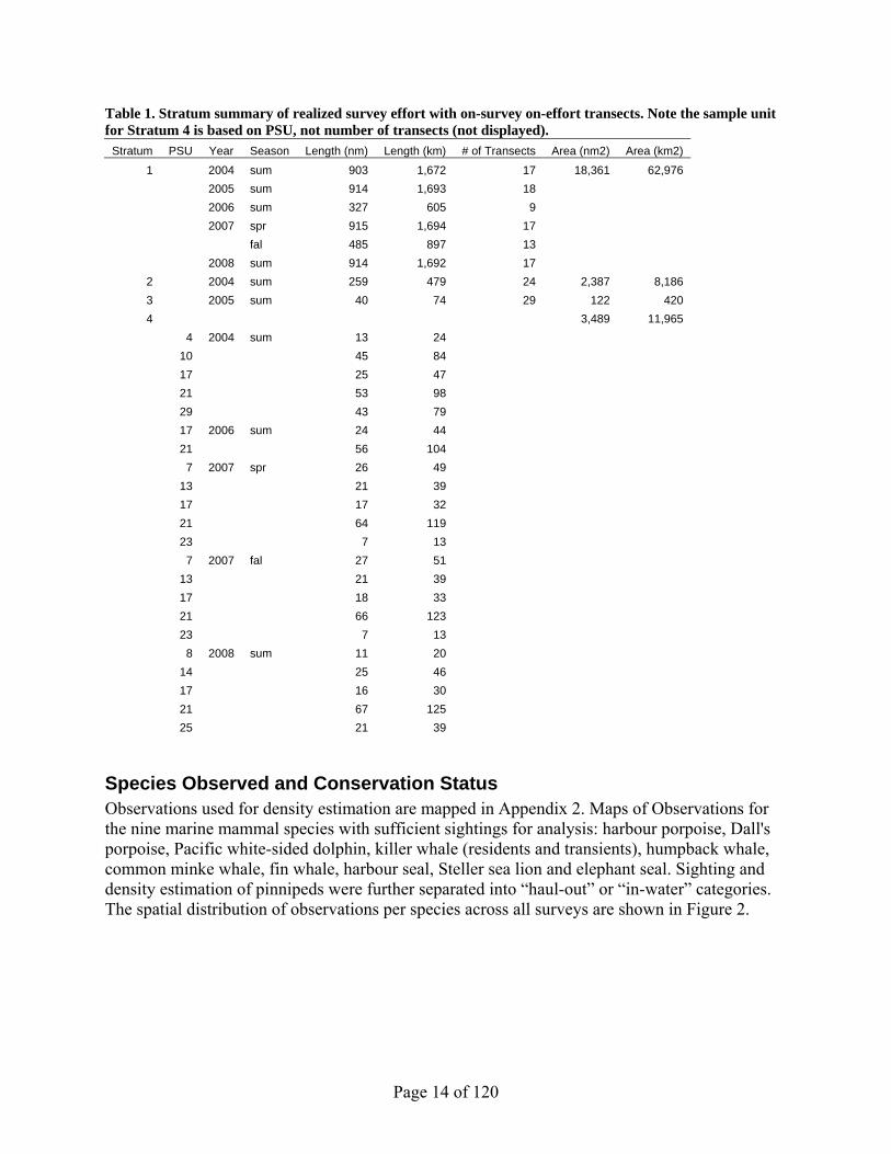
List of Tables Table 1. Stratum summary of realized survey effort with on-survey on-effort transects. Note the
sample unit for Stratum 4 is based on PSU, not number of transects (not displayed)...... 14
Table 2. Conservation status of marine mammals in British Columbia waters. Provincial BC status ranges from imperiled (S2) to secure (S5), and not applicable (SNA). Additional criteria, such as subpopulations for killer whales or breeding versus non-breeding status are specified by this criteria in some instances. National COSEWIC status ranges from Endangered (E) to Threatened (T) to Special Concern (SC) to not at risk (NAR). The IUCN status ranges from Endangered (EN) to Least Concern (LC), and data deficient (DD). Year assessed in paranthesis................................................................................... 17
Table 3. Detection function summary statistics. Truncation distance (w) with number of sightings (n) before and after truncation. Model described by key function (hazard-rate (hr), half-normal (hn), or uniform (un)) with optional series expansion terms (polynomial (poly), or cosine (cos)). The p-value for the goodness-of-fit Kolmogorov-Smirnov (K-S), and the final probability of detection p and its percent coefficient of variation (%CV ( p )). ..... 22
Table 4. Estimated school size...................................................................................................... 24
Table 5. Conventional distance sampling estimates for cetaceans in Stratum 1. ......................... 28
Table 6. Conventional distance sampling estimates for cetaceans in Strata 2,3,4, and entire region. ............................................................................................................................... 29
Table 7. Conventional distance sampling estimates for pinnipeds in Stratum 1. ......................... 30
Table 8. Conventional distance sampling estimates for pinnipeds in Strata 2,3,4, and entire region. ............................................................................................................................... 31
Table 9. Generalized Additive Model (GAM) formulation with truncation distances (w) and distance model type (Detection) for given stratum with generalized cross-validation score (GCV), deviance explained and GAM model terms. * terms were limited to 5 knots ...... 40
Table 10. Cetacean abundance estimates derived from the density surface models. ................... 43
Table 11. Pinniped abundance estimates derived from the density surface models. .................... 44
Table 12. Distances of routes in km. For the oil transportation example in and out of the Kitimat port only the conservation surface is used for generating the least-cost route, compared to the industry-proposed route and Euclidean path. The cruise ship industry path comes from existing routes, the distance from which is summed with the conservation surface to provide the total cost surface with which to route the least-cost path. Since the cruise ship route splits, the distance for the one going up Principe Channel is shown....................... 55

Page 11 of 120
Introduction to the Project Characterizing the distribution and abundance of protected species is essential to more objectively assess the risk factors related to potentially adverse interactions with human activities. Although information on animal distribution and abundance is integral to wildlife conservation and management, surprisingly few data on marine mammal distribution and abundance have been collected in the waters of Canada’s Pacific coast (Ban et al. 2008). Accordingly, spatial distribution and abundance of marine mammals in this region is poorly described. In addition, there has been little work examining and comparing the habitat preferences of different species. Although killer whales in this region are particularly well studied, abundance estimates and distribution information is not available for most cetacean and pinniped species inhabiting the region, including those species that were heavily depleted by commercial exploitation. Our goal is to build regional multi-species models that help to understand the environmental factors that influence marine mammal abundance and distribution. The habitat preferences of a species represent an important part of a species niche (Guisan and Zimmermann 2000). Although a species distribution may change in the short-term as local conditions change, its niche is likely to remain unchanged (Martínez-Meyer, Townsend Peterson, and Hargrove 2004). Therefore, an understanding of a species niche can be used to predict how a species will react to changes in its local environment over time. This is particularly important considering the likelihood of increased anthropogenic impacts in our study area, which heightens the urgency to collect baseline data on marine mammal distribution and abundance. In recent years, for example, there has been considerable discussion about lifting existing moratoria on offshore oil and gas exploration and extraction off the north and central coasts of BC (Royal Society of Canada 2004). Such changes have implications for how species interact with human activities and for determining the best approaches to the conservation and management of marine mammal populations and species. The nearshore waters of British Columbia are home to a diverse suite of marine mammals, some of whose endangered status is threatened by human activities. Whereas the Species at Risk Act (SARA) has afforded these animals protections and some conservation efforts are in place, existing and expanding activities from transportation, oil, wind, and fisheries industries may adversely impact these species (Government of British Columbia 2006; Ban & Alder 2008). Quantifying the temporal trends and spatial distribution of their abundance is essential for conservation management. The Raincoast Conservation Foundation has conducted marine mammal surveys in the nearshore BC waters between 2004 and 2008, predominately during summer, but also during spring and fall. Using the first two years of data, Williams and Thomas (2007) first characterized the abundance of marine mammals across 4 strata using design-based estimates, which assumes homogenous density within strata. Herein, we update these stratum-based estimates with subsequent years of survey effort and look at abundance across years and seasons. We then employ density surface modeling with environmental covariates to produce maps that describe the spatially heterogeneous distribution of animal density across the study area. These density surfaces are then composited into a single marine mammal hotspot map, which can be used to

Page 12 of 120
reduce risk for site-specific activities. This composite map is finally used as a cost surface for suggesting a framework to route vessel traffic around sensitive areas.
Survey Design Marine mammal surveys were conducted across the inner waters of British Columbia during the summers of 2004, 2005, 2006, and 2008 and during spring and fall for 2007. The surveys were designed to maximize coverage and minimize off-effort time over 4 strata (Figure 1) for the purposes of design-based multi-species density estimation according to Thomas et al. (2007). Zigzag configurations were applied over the open strata (1 and 2), with sub-stratification for the more topographically complex strata 2. For the narrower strata (3 and 4), parallel lines oriented perpendicular to the long axis minimized edge effects. The inlet strata (4) were further subdivided into primary sampling units (PSUs) so that for a given season, a random subsample of PSUs was selected for surveying. Total effort by length and number of transects per year and season of survey is given in Table 1. To estimate density, effort-weighted means were used for all strata, except stratum 4 which was derived from the unweighted mean of the PSUs.

Page 13 of 120
Figure 1. Stratum ID and on-effort transects, including transit legs between design-based transects, for all years, corresponding to Queen Charlotte Basin (1), Straits of Georgia and Juan de Fuca (2), Johnstone Strait (3), and mainland inlets (4).
Page 14 of 120
Table 1. Stratum summary of realized survey effort with on-survey on-effort transects. Note the sample unit for Stratum 4 is based on PSU, not number of transects (not displayed).
Stratum PSU Year Season Length (nm) Length (km) # of Transects Area (nm2) Area (km2) 1 2004 sum 903 1,672 17 18,361 62,976
2005 sum 914 1,693 18 2006 sum 327 605 9 2007 spr 915 1,694 17 fal 485 897 13 2008 sum 914 1,692 17
2 2004 sum 259 479 24 2,387 8,186 3 2005 sum 40 74 29 122 420 4 3,489 11,965
4 2004 sum 13 24 10 45 84 17 25 47 21 53 98 29 43 79 17 2006 sum 24 44 21 56 104 7 2007 spr 26 49 13 21 39 17 17 32 21 64 119 23 7 13 7 2007 fal 27 51 13 21 39 17 18 33 21 66 123 23 7 13 8 2008 sum 11 20 14 25 46 17 16 30 21 67 125 25 21 39
Species Observed and Conservation Status Observations used for density estimation are mapped in Appendix 2. Maps of Observations for the nine marine mammal species with sufficient sightings for analysis: harbour porpoise, Dall's porpoise, Pacific white-sided dolphin, killer whale (residents and transients), humpback whale, common minke whale, fin whale, harbour seal, Steller sea lion and elephant seal. Sighting and density estimation of pinnipeds were further separated into “haul-out” or “in-water” categories. The spatial distribution of observations per species across all surveys are shown in Figure 2.

Page 15 of 120
Figure 2. Observations by species from all surveys. The conservation status of species are determined globally by the United Nations body the International Union for Conservation of Nature (IUCN) and within Canada by the Committee on the Status of Endangered Wildlife in Canada (COSEWIC). The government of British Columbia also designates conservation status locally within the province. The status of the marine mammal species assessed in this study are listed in

Page 16 of 120
. Many of the threats to marine mammals are shared across species: low populations from historical hunting, incidental catch from fishing gear, depletion of prey from overfishing, chemical pollution, vessel strikes, and ship noise (Rice 1998).

Page 17 of 120
Table 2. Conservation status of marine mammals in British Columbia waters. Provincial BC status ranges from imperiled (S2) to secure (S5), and not applicable (SNA). Additional criteria, such as subpopulations for killer whales or breeding versus non-breeding status are specified by this criteria in some instances. National COSEWIC status ranges from Endangered (E) to Threatened (T) to Special Concern (SC) to not at risk (NAR). The IUCN status ranges from Endangered (EN) to Least Concern (LC), and data deficient (DD). Year assessed in paranthesis.
Provincial National Global BC Status COSEWIC IUCN Status
Harbour porpoise S3 (2006) SC (2003) LC (2008) Dall's porpoise S4S5 (2006) NAR (1989) LC (2008) Pacific white-sided dolphin S4S5 (2006) NAR (1990) LC (2008) Humpback whale S3 (2006) T (2003) LC (2008) Fin whale non-breeding S2 (2006) T (2005) EN (2008) Killer whale (res+trans) offshores S3 (2006)
transients S2 (2006) S residents S2 (2006)N residents S3 (2006)
T (2008)T (2008)E (2008)T (2008)
DD (2008)
Minke whale non-breeding S4 (2006) NAR (2006) LC (2008) Harbour seal S5 (2006) NAR (1999) LC (2008) Steller sea lion breeding S2S3 (2006)
non-breeding S3 (2006)SC (2003) EN (2008)
Elephant seal SNA (2006) NAR (1986) LC (2008)
Harbour Porpoise The Harbour porpoise (Phocoena phocoena) is listed as Vulnerable by the IUCN with a global population estimate of about 700,000 individuals (Hammond et al. 2008a). Within Canadian Pacific waters, it is recognized as a species of Special Concern (COSEWIC 2003). Found predominantly in shallow waters less than 200m in the Northern Hemisphere, 4 subspecies have been genetically identified globally (Rice 1998). Despite continuous distribution alongshore from Point Conception around the Pacific rim to the northern islands of Japan and as far north as Barrow, Alaska, many small populations appear genetically distinct, suggesting the need to consider small subpopulation management units (Chivers et al. 2002). Prior to the study conducted by Williams & Thomas (2007), the only distribution information estimated 3,000 individuals for the southern inshore portion of BC based on 1996 surveys (Baird 2003a). To the south, the stock in the coastal waters of Washington and Oregon were estimated to be around 40,000 in 1997, and to the north in southeastern Alaska to be 10,000 animals (Baird 2003a).
Dall's porpoise The Dall’s porpoise (Phocoenoides dalli) is globally abundant with an estimated population of over 1.2 million individuals and listed as a species of Least Concern by the IUCN (Hammond et al. 2008b) and not at risk within Canada. They are distributed within the North Pacific Ocean, generally in deeper waters between 30°N and 62°N (Jefferson 1988). Considered either a subspecies or color-morph the most common dalli-type resides in the NW Pacific.

Page 18 of 120
Pacific white-sided dolphin The Pacific white-sided dolphin (Lagenorhynchus obliquidens) is listed by the IUCN as a species of Least Concern with global populations estimated to be over 1 million (Hammond et al. 2008c) and not at risk in Canadian waters. They are distributed along the temperate coastal shelf waters and some inland BC waterways of the North Pacific from roughly 35°N to 47°N (Stacey and Baird 1991; Heise 1997).
Humpback whale Humpback whales (Megaptera novaeangliae) were down-listed by the IUCN in 2008 to a species of Least Concern status since current global estimates now exceed 60,000 individuals. This population level exceeds the 50% threshold of the 1940 population needed to retain its former Vulnerable status (Reilly et al. 2008a). Combined mark-recapture and photo-id analysis conducted under the “Structure of Populations, Levels of Abundance and Status of Humpback Whales in the North Pacific” (SPLASH) project estimate the population in the region to be just under 20,000, which is appoximately double the previous population estimates (Calambokidis et al. 2008). These increasing numbers have been heralded as a sign of post-whaling recovery (Dalton 2008). In southeastern Alaska, Dahlheim et al. (2009) found that humpback whale abundance over the period 1991 to 2007 increased annually by 10.6% (SE=0.015). The Canadian and Provincial designations, Special Concern (S3) and Threatened (T) respectively (Baird 2003b), have not been updated since 2006 and 2003.
Fin whale The Endangered fin whales (Balaenoptera physalus) are found globally, largely in offshore waters and less so in warm tropical regions (Reilly et al. 2008b). They are noted to occur on the middle (50–100 m) and outer shelves (100–200 m) in the eastern Bering Sea (Moore et al. 2002). In the waters off of western Alaska and the central Aleutian Islands, Zerbini et al. (2006) compared surveys from 1987 with those from 2001-2003 and found a 4.8% (95% CI = 4.1-5.4%) annual rate of increase (Zerbini et al. 2006) with population levels at 1652 (95% CI = 1142-2389) individuals. Since the 1975 north Pacific estimate of roughly 17,000 fin whales, down from an estimated 44,000 preceding intensive whaling, there has been a lack of sufficient survey data and abundance estimates (Reilly et al. 2008b) to develop estimates for the entire regional population of fin whales.
Killer whale Killer whales (Orcinus orca) occur globally in highly productive, often cooler waters, and are listed by the IUCN as Data Deficient (Taylor et al. 2008). In British Columbia there are four designated units of killer whales (with 2006 population estimates based on photo-id): 1) Northern Resident (244), 2) Southern Resident (87), 3) West Coast Transient (198), and 4) Offshore (COSEWIC 2008). All of these subunit populations are designated within Canadian waters as Threatened, except the southern residents, which are listed as Endangered. These subunit populations generally do not interact with each other, have unique habitats, forage for different prey, and can generally be identified by dorsal fin morphology (Ford et al. 2009). The residents feed on fishes, especially salmon, while the transients prey on marine mammals. The less understood offshore type probably also feed on fish, although different varieties than the transients based on stable isotope analysis (Ford et al. 2009).

Page 19 of 120
Minke whale Minke whales (Balaenoptera acutorostrata) are found globally and are listed as a species of Least Concern despite no global estimates since estimates for parts of the Northern Hemsiphere alone are over 100,000 (Reilly et al. 2008c). In Canada they are listed as a species Not at Risk.
Harbour seal Harbour seals (Phoca vitulina) inhabit the coastal parts of the Northern Hemisphere in temperate and polar areas with a global population between 350,000 to 500,000 individuals (Thompson and Härkönen 2008), and have an IUCN status of species of Least Concern and are considered Secure in Canada. Of the five subspecies, P.v. richardii is found in the eastern Pacific, which has been stable or increasing in population since the early 1990s.
Steller sea lion Steller sea lions (Eumetopias jubatus) inhabit the coastal waters of the North Pacific. They experienced a dramatic 64% decline in their population from 1960 to 1989, with a current estimate of 105,000 to 117,000 animals (Gelatt and Lowry 2008). Recognized as a species of Special Concern in British Columbia, they are found near one of three breeding grounds and 21 haul-out sites. The BC breeding population is estimated to be about 19,000 animals, out of the total Eastern population estimated to be 45,000 individuals in 2002 (COSEWIC 2003).
Elephant seal Elephant seals (Mirounga angustirostris) have recovered from virtual extinction with 2005 population estimates around 171,000 and are now listed by the IUCN as a species of Least Concern. Elephant seals range from throughout the northeastern Pacific (Campagna 2008). Within Canada’s waters they are considered Not at Risk.
Abundance Estimation Estimating the abundance of marine mammal species requires specialized techniques to objectively extrapolate from individual point observations of animals collected along line-transect surveys to broader estimates of the expected encounter rate, abundance and density. Since many marine animals are only observed at the surface for short intervals and the ability of observers is significantly influenced by sea conditions, modeling techniques must also specifically estimate the expected probability of detection (Buckland et al. 2001; Burnham et al. 1980). Traditional estimates of cetacean abundance have relied on design-based surveys covering an entire survey strata at a time and have been based on simple estimates of the detection function (Buckland et al. 2001). More recently, detection functions have been fitted using environmental covariates to provide more precise estimates (Marques and Buckland 2003). For instance, Barlow and Forney (2007) used covariates such as glare, group size and survey vessel as detection function covariates to analyze the most comprehensive set of multi-species cetacean surveys to date for the US West Coast. Even more recently, a spatial modeling component has been in development for inclusion in the Distance software (Thomas et al. 2006). Ferguson et al. (2006) used similar techniques in the Eastern Tropical Pacific to predict both encounter rates and group sizes of cetacean species using generalized additive models to link with environmental

Page 20 of 120
covariates. They tested for geographic pattern in the unexplained model residuals to control for potential autocorrelation. These methods help provide more precise and object estimates of habitat preferences. Regression-based techniques are the most common methods for determining habitat preferences of cetaceans (Redfern et al. 2006), and of these generalized additive models have the most flexibility for determining non-linear relationships. Here we use the conventional stratum-based abundance estimation with a covariate of group size and compare with the more advanced density surface, or spatial modeling, approaches using generalized additive models to estimate encounter rate.

Page 21 of 120
Tier A. Estimating Abundance
Product 1. Using Conventional Distance Sampling
Methods The design-based abundance methods of Williams and Thomas (2007) originally performed on 2004 and 2005 data were reproduced for the extended period of survey to include 2006, 2007 and 2008 data for comparison. Abundance is is estimated as the density of animals multiplied by
the applicable study area or stratum. To estimate density ( D ) the encounter rate (Ln ), or number
of schools seen (n) over the length of the transect (L), is multiplied by twice the truncation distance (w) to obtain an area and the estimated school size ( s ). ˆ D = nˆ s
L2wˆ p (1)
If all animals present within the transect area were assumed to be detected over this area, as with strip transects, we would stop here. However, we can safely assume that the probability of detecting a school decreases with distance. Accounting for this probability of detection ( p ) forms the basis of ‘conventional distance sampling’ (CDS), formally described by Buckland et al. (2001) by fitting a detection function (covered in the next section). This p term in the denominator allows for the probability of detection to decrease with distance and the estimate of density will be appropriately compensated.
Detection Functions Detection functions were estimated using the software Distance 6.0 Beta 3 (Thomas et al, 2006), which can apply several key functions (uniform, half-normal or hazard rate) and series expansion terms (polynomial or cosine) to estimate the shape of the function. The observers recorded radial distance (d) and angle (θ) during the field surveys. These relative values are then converted to perpendicular distance from the trackline using simple geometry, sin(θ)*d. All on-effort (i.e. periods when the observers were actively observing for animals) sightings, including off-transect observations, were used for detection model fitting. Models were generally selected that minimize the Akaike Information Criterion (AIC) score, which promotes explanation of deviance while penalizing the addition of terms to achieve the most parsimonious model (Akaike 1974). In addition, the Kolmogorov-Smirnov goodness-of-fit test was employed to provide a measure of agreement between the model and data (S. T. Buckland et al. 2004). If species exhibit an attraction to the survey vessel, then a spike is typically seen nearest the trackline which can inflate the density estimates by lowering the p over the rest of the strip width. As detectability drops off, inclusion of further distances in the function can similarly inflate the density so a reasonable truncation distance (w), usually excluding the furthest 5% or 10% of the observations is selected and is then rounded to the nearest 100m. These detection functions all assume perfect detection on the trackline, i.e. g(0)=1. A probability of availability is typically divided by the density to account for the fact that marine mammals are

Page 22 of 120
often below the water surface and not detected even when directly on the trackline of the observer vessel. Estimating this probability requires tracking of individuals to estimate proportion of time spent underwater (Laake et al. 1997) or multiple platforms of simultaneous, independent observation. These time and cost-intensive estimates have not yet been conducted for these species in these waters, and so are not applied. Therefore the abundance estimates developed may underestimate the true population size.
School Size School size, or group size, was estimated in Distance using the default conventional distance sampling method. We expect that the estimate of school size diminishes with observed distance, e.g. school sizes tend to be underestimated when observed from a further distance. The natural logarithm of group size is regressed on the probability of detection, and the value of ln( s ) at zero distance is back-transformed to obtain the estimated school size ( s ).
Results The final detection models selected are given in Table 3. Observations are truncated to within the perpendicular distance (w) used by the conventional distance sampling (CDS) methods for comparison (see Appendix 2. Maps of Observations). Table 3. Detection function summary statistics. Truncation distance (w) with number of sightings (n) before and after truncation. Model described by key function (hazard-rate (hr), half-normal (hn), or uniform (un)) with optional series expansion terms (polynomial (poly), or cosine (cos)). The p-value for the goodness-of-fit Kolmogorov-Smirnov (K-S), and the final probability of detection p and its percent coefficient of variation (%CV ( p )).
w (m) n before n after Model K-S p p %CV ( p )Harbour porpoise 600 128 118 (-8%) hr 0.899 0.201 24.29Dall's porpoise 700 239 221 (-8%) hn+cos(3) 0.190 0.344 9.86Pacific white-sided dolphin 1200 233 219 (-6%) hn+cos(4) 0.001 0.253 8.63Humpback whale 2300 352 325 (-8%) hn+cos(1) 0.951 0.421 6.43Fin whale 3900 91 82 (-10%) hn+cos(2) 0.375 0.270 11.01Killer whale (res+trans) 1300 29 25 (-14%) hn 0.302 0.558 16.71Minke whale 400 32 29 (-9%) un+cos(1) 0.641 0.620 13.81Harbour seal (haul-out) 700 244 212 (-13%) un+cos(1) 0.326 0.728 6.69Harbour seal (in-water) 500 774 732 (-5%) hn+cos(1) 0.030 0.477 4.74Steller sea lion (haul-out) 1300 20 17 (-15%) un+cos(1) 0.639 0.686 21.57Steller sea lion (in-water) 500 123 114 (-7%) hn 0.047 0.548 7.71Elephant seal 500 20 18 (-10%) un 0.572 1.000 0.00

Page 23 of 120
Figure 3. Detection functions for conventional distance sampling (CDS) analysis.

Page 24 of 120
Table 4. Estimated school size. Estimated school size Observed school size
s %CV ( s ) Mean %CV Maximum Harbour porpoise 1.67 4.56 1.81 4.53 5 Dall's porpoise 2.41 4.54 2.43 5.55 15 Pacific white-sided dolphin 13.53 14.77 38.27 20.41 1200 Humpback whale 1.51 2.79 1.57 3.75 8 Fin whale 1.78 6.86 1.99 12.73 20 Killer whale (res+trans) 3.67 18.26 3.80 15.27 28 Minke whale 0.99 2.36 1.03 3.33 2 Harbour seal (haul-out) 5.58 9.51 6.82 9.77 90 Harbour seal (in-water) 1.11 1.20 1.20 2.83 18 Steller sea lion (haul-out) 70.29 66.86 37.77 49.25 300 Steller sea lion (in-water) 6.11 20.31 14.41 26.89 370 Elephant seal 1 0 1 0 1
Cetaceans
Harbour porpoise Combining all surveys, 128 harbour porpoise schools were sighted (Table 3). They are distributed widely across the northern and southern extents of the study area, and are found to be more common nearshore and within inlets (Figure 2). The vast majority (122/128=95%) exhibited traveling/foraging behaviour, and only 2 feeding and 2 avoiding, so no obvious response to the observer vessel is indicated with this data.. Restricting the observations to a truncation distance of 600m excluded 10 observations, or 8% of the data collected (Table 3). The most parsimonious detection function as determined by the lowest AIC was the hazard rate model without adjustment terms (Figure 3). The data show a spike near zero, which is most appropriately fit with a hazard rate model. These spikes are typically of concern with attractive movement, but none was noted in the field, so alternate models that removed the spike were not chosen over the lower AIC criteria. The bias towards zero in the detection function may accurately reflect the small size and cryptic nature of this species. All the other models tested with higher AIC values produced smoother fits than the data or the hazard rate model, which produced a higher p and lower abundance estimate. For instance, the next lowest-AIC model (ΔAIC=8.53), uniform with 5 cosine adjustments, produced a p 41% larger (0.284 vs 0.201).
Dall’s porpoise Of the 239 Dall’s porpoise school sightings (Table 3), most occurred in the northern and southern ends of Queen Charlotte Basin, often offshore within the basin, with relatively few schools within the inlets or the southern straits (Figure 2). Whereas most observations (212/239 = 88.7%) were traveling/foraging, a noteworthy portion (11/239 = 4.6%) were approaching and the same number feeding. Other behaviours included schooling (2/239 = 0.8%), avoiding (1/239 = 0.4%) and unknown (2/239 = 0.8%). A truncation distance of 700m excluded 18 observations, or 8% of the observations from model fitting. The hazard rate function with 1 cosine adjustment fit the data best according to the AIC

Page 25 of 120
crietria, but exhibited a sharp spike near zero. Given that Dall’s porpoise were recorded with attractive behaviour and are known to bow-ride in front of boats, the next lowest-AIC model (ΔAIC=7.02), half-normal with 3 cosine adjustments, was chosen because of it’s broader shoulder which minimizes the bias near zero due to attractive behaviour (Figure 3). Turnock and Quinn (1991) also found that a half-normal corrects most for the attractive aspects, using simulations and data from Dall’s porpoises in Alaska. To further quantify a correction factor, a secondary platform of observation is recommended.
Pacific white-sided dolphin Of the 233 schools of Pacific white-sided dolphin, the majority were seen throughout the southern half of the Queen Charlotte Basin, particularly near Haida Gwaii, as well as a few observations in the inlets and northern end of the southern straits (Figure 2). This species exhibits the strongest approaching behaviour (47/233=20.2%). Other behaviours include: traveling/foraging (151/233=64.8%), feeding (18/233=7.7%), breaching (13/233=6%), socializing (1/233=0.4%), avoidance (1/233=0.4%) and uncertain (2/233=0.8%). Using a truncation distance of 1200m (Table 3), the lowest-AIC models used a hazard rate model, which followed the spike of the data near zero distance. To minimize the bias of attractive movement, the next lowest-AIC (ΔAIC=23.89) half-normal model with 4 cosine adjustments was chosen (Figure 3). This is a similar strategy for model selection as used with Dall’s porpoise.
Humpback whale The highest number of cetacean school sightings (n=352) were attributed to humpback whale (Table 3). These sightings occurred exclusively in Queen Charlotte Sound and the inlets, and not in the southern straits (Figure 2). Most Sound sightings were in deep water, with some preference towards the southern Haida Gwaii region and the northeastern Sound. Only one observation was noted for approaching behaviour (1/352=0.2%), and the rest included: traveling/foraging (265/352=75.3%), feeding (41/352=11.6%), breaching (25/352=7.1%), socializing (3/352=8.5%), and unknown (5/352=1.4%). Using a 2300m truncation distance, the lowest-AIC model was chosen using a half-normal model with one cosine adjustment term (Figure 3).
Fin whale All of the 91 school sightings of fin whale were found in Queen Charlotte Basin, with the exception of a couple of observations in the Grenville Channel inlet. Historical records reveal that fin whales were once one of the most abundant and heavily whaled marine mammals within the inshore waters British Columbia (Gregr et al. 2000). Most these sightings are in the southern end of the Queen Charlotte Islands, with another large cluster of sightings are in the north of the Sound (Figure 2). The behaviours of sightings include: traveling/foraging (73/91=80.2%), feeding (3/91=3.3%), socializing (1/91=1.1%), and other/uncertain (4/91=4.4%). A 3,900m truncation distance was applied (Table 3). The hazard rate model obtained the lowest AIC, but exhibited a spike near zero, so a half-normal model with two cosine adjustment terms (ΔAIC=1.4) was used instead (Figure 3).
Killer whale

Page 26 of 120
At 29 school sightings, the killer whale is the least common of the observed whale species (Table 3), but one of the most studied species. Most targeted killer whale studies differentially treat the resident versus transient ecotypes (Zerbini et al. 2007), but data constraints forced us to lump the two types together for this analysis. Sightings occurred in both Queen Charlotte Basin and Johnstone Strait, most commonly near shore (Figure 2). Observed behaviours include: traveling/foraging (24/29=82.7%), feeding (2/29=6.7%), socializing (1/29=3.4%) and other (2/29=6.7%). A truncation distance of 1300m was applied to provide a monotonically decreasing tail, while retaining as many observations as possible (25/29=86%). A hazard rate model best fit these data. But to offset the spike near zero, the half-normal model without adjustment terms (ΔAIC=0.53) was chosen.
Minke whale Only slightly more common (n=32) than killer whales in school sightings is the common minke whale (Table 3). All observations were widely distributed within Queen Charlotte Basin, generally offshore in deeper waters (Figure 2). All sightings were recorded as traveling/foraging behaviour, although minke whales are at surface less than other species so directionality is often difficult to determine. Of the 32 observations only 3 exceeded 400 m in perpendicular distance from the transect line (2377 m, 1888 m, and 1532 m), so a truncation distance of 400m was used. The lowest-AIC model, a uniform model with one cosine adjustment term, was chosen in this case.
Pinnipeds
Harbour seal The most commonly sighted of all marine mammals (n=1018), the harbour seal was seen most typically nearshore throughout all strata: sound, inlets, and straits (Figure 2). Harbour seals exhibited the following behaviours: traveling/foraging (701/1018=68.9%), socializing (75/1018=7.4%), feeding (13/1018=1.3%), approaching (1/1018=0.1%), and other/unknown (110/1018=10.8%). Detectability is expected to vary as a function of whether the pinniped is in or out of water, hence the separation between in-water and haul-out observations for truncation distances and detection functions (Table 3). For in-water observations, a truncation distance of 500m was used and the lowest-AIC model selected was a half-normal model with one cosine adjustment term (Figure 3). For haul-out observations, a 700m truncation was used, indicative of greater visibility when out of water, and the lowest-AIC model selected was a uniform model with one cosine adjustment. The distance data for haul-out observations exhibit a peak around 200m rather than monotonically increasing towards zero. Because most haul out sightings are to the side during along-shore transects, this off-zero peak is understandable. Roughly one quarter of the sightings were haul-out versus three quarters in-water.
Steller sea lion A total of 123 Steller sea lion schools were sighted in-water and 20 on land, all generally in the nearshore and inlet environments of the southern Queen Charlotte Basin (Figure 2). They exhibited slight responsiveness to the ship (avoidance: 3/123=24.4%; approach: 2/123=1.6%), otherwise found traveling/foraging (67/123=54.5%), socializing (10/123=8.1%), feeding (3/123=2.4%), or other/unknown (38/123=30.9%). For in-water observations, a 500m truncation distance was used and the lowest-AIC model selected was a half-normal model. For haul-out

Page 27 of 120
observations, a 1300m truncation distance was used and the lowest-AIC model selected was a uniform model with one cosine adjustment.
Elephant seal The least numerous of all the marine mammal species analyzed here (# school sightings=20), the elephant seal was observed in the open waters of Queen Charlotte Basin as well as the southern and central inlets (Figure 2). A 500m truncation distance was used, and the final model selected was a uniform model, which corresponds to a strip transect, i.e. density is assumed to not vary with distance from transect. In this case there were too few observations to construct a robust distance detection function, further evidenced by the unrealistic p value of a solid 1 (Table 3).
Abundance Estimates Abundance estimates were calculated across all surveyed seasons and strata by species, as summarized by Tables 5 through 8. During the 2006 survey, observer effort within the inlet stratum 4 was not part of a designed survey and only included effort while on passage, so this data was excluded for estimation of abundance estimates. Comparing this analysis with previous estimates (Williams and Thomas 2007), which used only survey data from 2004 and 2005; we see closer confidence intervals for the results of the overall surveyed region with the addition of recent survey data. Steller sea lions and elephant seals were included in this analysis and not in Williams and Thomas (2007) due to limited sample size.

Page 28 of 120
Table 5. Conventional distance sampling estimates for cetaceans in Stratum 1. Stratum 1 2004 2005 2006 2007 2007 2008 Average Average Estimate Summer Summer Summer Spring Fall Summer All Summers Harbour porpoise D 0.157 0.309 0 0.056 0.027 0.211 0.153 0.202 95%CI(D) 0.036 - 0.675 0.108 - 0.887 0 0.014 - 0.221 0.003 - 0.216 0.044 - 1.023 0.066 - 0.355 0.083 - 0.492 N 2,874 5,677 0 1,032 487 3,874 2,806 3,704 95%CI(N) 667 - 12,391 1,980 - 16,279 0 263 - 4,054 60 - 3,964 799 - 18,785 1,209 - 6,514 1,518 - 9,040 %CV 79.4% 54.9% 0 73.4% 125.1% 87.5% 43.2% 45.9% Dall's porpoise D 0.492 0.354 0.113 0.081 0.115 0.182 0.247 0.318 95%CI(D) 0.248 - 0.978 0.109 - 1.152 0.039 - 0.332 0.027 - 0.240 0.035 - 0.379 0.085 - 0.391 0.147 - 0.416 0.180 - 0.560 N 9,038 6,507 2,083 1,487 2,105 3,350 4,540 5,838 95%CI(N) 4,549 - 17,956 2,001 - 21,159 711 - 6,098 503 - 4,399 638 - 6,950 1,562 - 7,184 2,700 - 7,632 3,313 - 10,289 %CV 33.8% 60.9% 50.1% 55.1% 59.7% 37.7% 25.5% 27.8% Pacific white-sided dolphin D 2.196 1.762 3.415 0.858 0.085 1.582 1.566 2.013 95%CI(D) 1.048 - 4.600 0.544 - 5.705 1.107 - 10.536 0.387 - 1.901 0.007 - 1.041 0.745 - 3.361 0.928 - 2.642 1.152 - 3.517 N 40,316 32,345 62,708 15,755 1,565 29,054 28,759 36,958
95%CI(N) 19,243 - 84,464
9,988 - 104,747
20,327 - 193,448 7,111 - 34,905 128 - 19,113
13,680 - 61,706
17,047 - 48,517
21,153 - 64,573
%CV 37.2% 61.1% 53.9% 40.0% 166.2% 37.8% 26.4% 28.1% Humpback whale D 0.049 0.046 0.026 0.132 0.06 0.112 0.078 0.065 95%CI(D) 0.020 - 0.121 0.022 - 0.095 0.012 - 0.059 0.086 - 0.204 0.027 - 0.131 0.075 - 0.167 0.059 - 0.103 0.045 - 0.092 N 909 839 486 2,431 1,093 2,057 1,431 1,186 95%CI(N) 373 - 2,213 406 - 1,737 219 - 1,081 1,577 - 3,747 496 - 2,405 1,382 - 3,062 1,085 - 1,888 835 - 1,684 %CV 44.1% 35.7% 36.2% 21.0% 37.7% 19.3% 13.6% 17.0% Fin whale D 0.012 0.045 0 0.024 0.026 0.024 0.024 0.024 95%CI(D) 0.005 - 0.030 0.017 - 0.120 0 0.010 - 0.060 0.010 - 0.068 0.010 - 0.057 0.014 - 0.041 0.012 - 0.047 N 223 820 0 441 476 442 446 443 95%CI(N) 91 - 548 305 - 2,199 0 176 - 1,108 182 - 1,242 188 - 1,040 262 - 760 229 - 859 %CV 44.9% 50.0% 0 46.2% 47.1% 42.7% 26.4% 32.7% Killer whale D 0.026 0.01 0.014 0.015 0.01 0.005 0.014 0.014 95%CI(D) 0.007 - 0.100 0.002 - 0.045 0.003 - 0.073 0.005 - 0.050 0.001 - 0.138 0.001 - 0.025 0.006 - 0.032 0.005 - 0.036 N 476 188 263 282 177 94 251 253 95%CI(N) 124 - 1,829 43 - 829 51 - 1,346 86 - 921 12 - 2,527 19 - 463 107 - 585 96 - 666 %CV 72.0% 81.3% 83.6% 62.1% 186.3% 88.6% 43.4% 49.9% Minke whale D 0.029 0.02 0.045 0.02 0 0.02 0.022 0.025 95%CI(D) 0.014 - 0.058 0.007 - 0.055 0.015 - 0.136 0.007 - 0.061 0 0.005 - 0.078 0.013 - 0.037 0.014 - 0.045 N 526 371 830 371 0 371 396 466 95%CI(N) 258 - 1,071 136 - 1,013 275 - 2,505 123 - 1,119 0 96 - 1,431 231 - 678 261 - 829 %CV 35.4% 51.1% 52.1% 56.5% 0 71.2% 26.7% 28.6%

Page 29 of 120
Table 6. Conventional distance sampling estimates for cetaceans in Strata 2,3,4, and entire region. Stratum 2 Stratum 3 Stratum 4 Entire Region
Estimate 2004
Summer 2005
Summer 2004
Summer 2007
Fall&Spring 2008
Summer Average Average
Harbour porpoise D 1.342 0 0.24 0.049 0.247 0.178 0.272 95%CI(D) 0.540 - 3.334 0 0.006 - 9.643 0.001 - 1.616 0.006 - 9.903 0.012 - 2.709 0.138 - 0.536 N 3,203 0 838 170 861 622 6,631 95%CI(N) 1,289 - 7,957 0 21 - 33,641 5 - 5,639 21 - 34,546 41 - 9,449 3,366 - 13,065 %CV 47.4% 0 225.0% 317.2% 225.0% 213.6% 34.9% Dall's porpoise D 0.358 0.695 0.252 0.335 0.028 0.216 0.256 95%CI(D) 0.289 - 0.443 0.562 - 0.860 0.009 - 7.159 0.015 - 7.550 0.001 - 1.125 0.011 - 4.390 0.171 - 0.383 N 855 85 879 1,168 96 752 6,232 95%CI(N) 691 - 1,058 69 - 105 31 - 24,973 52 - 26,339 2 - 3,926 37 - 15,315 4,165 - 9,324 %CV 10.9% 10.9% 182.0% 238.4% 223.9% 267.7% 20.0% Pacific white-sided dolphin D 0.16 20.675 0 0.151 0.916 0.277 1.34 95%CI(D) 0.114 - 0.223 14.803 - 28.875 0 0.005 - 4.997 0.030 - 27.527 0.011 - 7.093 0.825 - 2.177 N 381 2,532 0 525 3,195 965 32,637 95%CI(N) 273 - 533 1,813 - 3,536 0 16 - 17,433 106 - 96,029 38 - 24,744 20,087 - 53,029 %CV 17.2% 17.1% 0 316.7% 189.2% 322.8% 24.6% Humpback whale D 0 0 0.062 0.004 0.047 0.031 0.063 95%CI(D) 0 0 0.002 - 1.711 0.000 - 0.145 0.004 - 0.615 0.002 - 0.436 0.049 - 0.082 N 0 0 216 15 164 110 1,541 95%CI(N) 0 0 8 - 5,967 0 - 505 13 - 2,146 8 - 1,521 1,187 - 2,000 %CV 0 0 178.5% 316.3% 117.1% 199.0% 12.9% Fin whale D 0 0 0 0 0 0 0.018 95%CI(D) 0 0 0 0 0 0 0.011 - 0.031 N 0 0 0 0 0 0 446 95%CI(N) 0 0 0 0 0 0 263 - 759 %CV 0 0 0 0 0 0 26.4% Killer whale D 0 0.469 0 0 0 0 0.013 95%CI(D) 0 0.287 - 0.766 0 0 0 0 0.006 - 0.027 N 0 57 0 0 0 0 308 95%CI(N) 0 35 - 94 0 0 0 0 146 - 649 %CV 0 24.8% 0 0 0 0 38.2% Minke whale D 0.014 0 0 0 0 0 0.018 95%CI(D) 0.011 - 0.019 0 0 0 0 0 0.011 - 0.029 N 34 0 0 0 0 0 430 95%CI(N) 26 - 45 0 0 0 0 0 259 - 712 %CV 14.0% 0 0 0 0 0 25.2%

Page 30 of 120
Table 7. Conventional distance sampling estimates for pinnipeds in Stratum 1.
Estimate 2004
Summer 2005
Summer 2006
Summer 2007
Spring 2007 Fall
2008 Summer
Average All
Average Summer
Harbour seal, hauled out
D 0.09 0.089 0.093 0.022 0.042 0.067 0.066 0.083 95%CI(D) 0.019 - 0.428 0.041 - 0.192 0.009 - 0.954 0.002 - 0.215 0.008 - 0.212 0.025 - 0.175 0.033 - 0.133 0.039 - 0.176 N 1,651 1,630 1,712 407 769 1,224 1,212 1,523 95%CI(N) 347 - 7,863 753 - 3,527 167 - 17,517 42 - 3,939 152 - 3,894 467 - 3,209 600 - 2,450 717 - 3,236 %CV 85.2% 38.4% 133.4% 146.7% 86.5% 48.4% 34.6% 37.2% Harbour seal, in water D 0.119 0.047 0.026 0.09 0.089 0.047 0.074 0.066 95%CI(D) 0.051 - 0.282 0.018 - 0.121 0.004 - 0.155 0.048 - 0.167 0.015 - 0.528 0.018 - 0.125 0.046 - 0.118 0.038 - 0.117 N 2,192 866 485 1,644 1,634 866 1,350 1,217 95%CI(N) 929 - 5,172 336 - 2,227 82 - 2,849 880 - 3,072 275 - 9,690 326 - 2,300 839 - 2,172 690 - 2,145 %CV 42.3% 47.2% 89.8% 30.3% 97.5% 48.7% 22.8% 27.3% Harbour seal, total D 0.209 0.136 0.12 0.112 0.131 0.114 0.14 0.149 95%CI(D) 0.089 - 0.491 0.075 - 0.246 0.019 - 0.750 0.053 - 0.235 0.035 - 0.495 0.057 - 0.226 0.093 - 0.210 0.092 - 0.241 N 3,842 2,496 2,197 2,052 2,403 2,090 2,562 2,740 95%CI(N) 1,638 - 9,016 1,379 - 4,516 350 - 13,778 974 - 4,323 635 - 9,087 1,052 - 4,154 1,704 - 3,852 1,697 - 4,426 %CV 43.8% 29.9% 105.8% 37.9% 71.9% 34.8% 20.3% 24.0% Steller sea lion, hauled out D 0 0 0 0 0.301 0.24 0.082 0.072 95%CI(D) 0 0 0 0 0.024 - 3.821 0.039 - 1.462 0.013 - 0.497 0.012 - 0.438 N 0 0 0 0 5,530 4,399 1,503 1,314 95%CI(N) 0 0 0 0 436 - 70,158 721 - 26,845 248 - 9,119 215 - 8,036 %CV 0 0 0 0 179.6% 109.6% 108.9% 109.6% Steller sea lion, in water D 0.16 0.135 0.063 0.316 0.17 0.158 0.18 0.142 95%CI(D) 0.038 - 0.664 0.060 - 0.307 0.012 - 0.334 0.132 - 0.758 0.052 - 0.553 0.059 - 0.422 0.098 - 0.333 0.067 - 0.297 N 2,936 2,485 1,160 5,797 3,126 2,901 3,314 2,601 95%CI(N) 706 - 12,200 1,096 - 5,634 219 - 6,129 2,415 - 13,914 963 - 10,145 1,087 - 7,746 1,796 - 6,116 1,239 - 5,460 %CV 76.7% 41.8% 85.1% 44.7% 60.0% 50.4% 31.3% 37.7% Steller sea lion, total D 0.16 0.135 0.063 0.316 0.471 0.398 0.262 0.213 95%CI(D) 0.038 - 0.664 0.060 - 0.307 0.012 - 0.334 0.132 - 0.758 0.071 - 3.117 0.114 - 1.388 0.121 - 0.567 0.091 - 0.498 N 2,936 2,485 1,160 5,797 8,656 7,301 4,817 3,915 95%CI(N) 706 - 12,200 1,096 - 5,634 219 - 6,129 2,415 - 13,914 1,309 - 57,235 2,092 - 25,483 2,230 - 10,403 1,675 - 9,153 %CV 76.7% 41.8% 85.1% 44.7% 116.8% 69.0% 40.2% 44.5% Elephant seal D 0.008 0.004 0 0.004 0 0 0.003 0.004 95%CI(D) 0.003 - 0.021 0.001 - 0.014 0 0.001 - 0.012 0 0 0.002 - 0.006 0.002 - 0.008 N 151 74 0 74 0 0 61 67 95%CI(N) 58 - 391 21 - 260 0 24 - 228 0 0 31 - 119 30 - 146 %CV 47.4% 64.9% 0 56.8% 0 0 32.0% 38.3%

Page 31 of 120
Table 8. Conventional distance sampling estimates for pinnipeds in Strata 2,3,4, and entire region.
Stratum 2 Stratum 3 Stratum 4 Entire Region
Estimate 2004
Summer 2005
Summer 2004
Summer 2007
Fall&Spring 2008
Summer Average Average
Harbour seal, hauled out D 1.217 0 1.567 0.3 1.437 0.844 0.29 95%CI(D) 0.968 - 1.529 0 0.090 - 27.386 0.033 - 2.773 0.059 - 34.745 0.067 - 10.642 0.225 - 0.374 N 2,904 0 5,467 1,047 5,014 2,944 7,060 95%CI(N) 2,311 - 3,649 0 313 - 95,538 113 - 9,673 207 - 121,210 233 - 37,126 5,477 - 9,101 %CV 11.7% 0 138.8% 128.1% 166.4% 185.0% 12.9% Harbour seal, in water D 1.934 0.647 1.631 1.225 0.902 1.246 0.427 95%CI(D) 1.754 - 2.133 0.588 - 0.713 0.134 - 19.808 0.220 - 6.830 0.088 - 9.234 0.240 - 6.480 0.375 - 0.485 N 4,617 79 5,689 4,275 3,145 4,348 10,394 95%CI(N) 4,187 - 5,090 72 - 87 468 - 69,099 767 - 23,827 307 - 32,212 836 - 22,606 9,143 - 11,816 %CV 5.0% 4.9% 111.8% 88.4% 101.2% 93.6% 6.5% Harbour seal, total D 3.151 0.647 3.198 1.526 2.339 2.09 0.717 95%CI(D) 2.832 - 3.506 0.588 - 0.713 0.553 - 18.492 0.373 - 6.237 0.303 - 18.047 0.424 - 10.309 0.631 - 0.814 N 7,521 79 11,156 5,322 8,159 7,292 17,454 95%CI(N) 6,760 - 8,367 72 - 87 1,929 - 64,510 1,302 - 21,757 1,057 - 62,957 1,479 - 35,964 15,362 - 19,831 %CV 5.4% 4.9% 88.7% 75.4% 109.4% 93.2% 6.5% Steller sea lion, hauled out D 0 0 0.323 0 0 0.073 0.072 95%CI(D) 0 0 0.009 - 11.304 0 0 0.002 - 2.923 0.013 - 0.391 N 0 0 1,126 0 0 256 1,759 95%CI(N) 0 0 32 - 39,433 0 0 6 - 10,196 324 - 9,534 %CV 0 0 234.4% 0 0 474.3% 99.9% Steller sea lion, in water D 0 0 0.261 0.43 0 0.271 0.175 95%CI(D) 0 0 0.013 - 5.410 0.022 - 8.249 0 0.015 - 4.804 0.101 - 0.301 N 0 0 910 1,499 0 946 4,260 95%CI(N) 0 0 44 - 18,874 78 - 28,777 0 53 - 16,760 2,472 - 7,341 %CV 0 0 155.6% 213.7% 0 240.4% 27.9% Steller sea lion, total D 0 0 0.583 0.43 0 0.345 0.247 95%CI(D) 0 0 0.051 - 6.618 0.022 - 8.249 0 0.024 - 4.860 0.125 - 0.487 N 0 0 2,035 1,499 0 1,202 6,019 95%CI(N) 0 0 179 - 23,087 78 - 28,777 0 85 - 16,956 3,056 - 11,853 %CV 0 0 147.1% 213.7% 0 214.5% 35.3% Elephant seal D 0 0 0 0.003 0 0.001 0.003 95%CI(D) 0 0 0 0.000 - 0.093 0 0.000 - 0.051 0.001 - 0.005 N 0 0 0 10 0 4 65 95%CI(N) 0 0 0 0 - 324 0 0 - 176 35 - 121 %CV 0 0 0 316.2% 0 469.0% 29.9%
Page 32 of 120
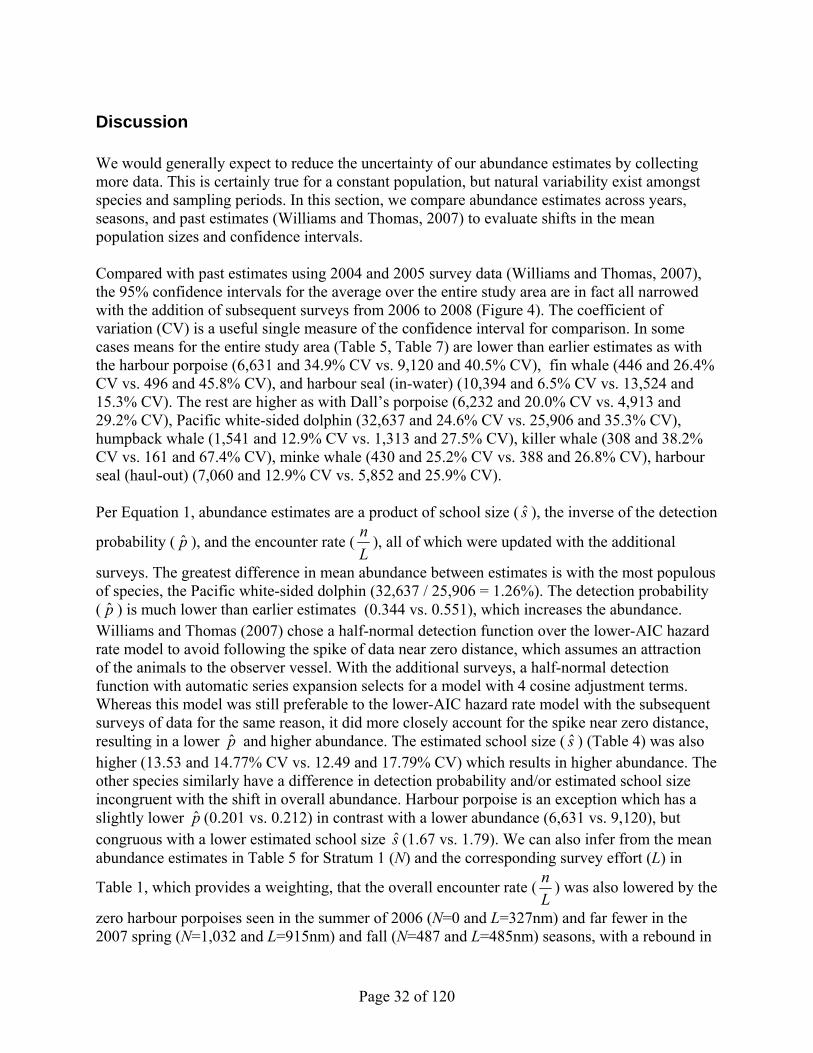
Discussion We would generally expect to reduce the uncertainty of our abundance estimates by collecting more data. This is certainly true for a constant population, but natural variability exist amongst species and sampling periods. In this section, we compare abundance estimates across years, seasons, and past estimates (Williams and Thomas, 2007) to evaluate shifts in the mean population sizes and confidence intervals. Compared with past estimates using 2004 and 2005 survey data (Williams and Thomas, 2007), the 95% confidence intervals for the average over the entire study area are in fact all narrowed with the addition of subsequent surveys from 2006 to 2008 (Figure 4). The coefficient of variation (CV) is a useful single measure of the confidence interval for comparison. In some cases means for the entire study area (Table 5, Table 7) are lower than earlier estimates as with the harbour porpoise (6,631 and 34.9% CV vs. 9,120 and 40.5% CV), fin whale (446 and 26.4% CV vs. 496 and 45.8% CV), and harbour seal (in-water) (10,394 and 6.5% CV vs. 13,524 and 15.3% CV). The rest are higher as with Dall’s porpoise (6,232 and 20.0% CV vs. 4,913 and 29.2% CV), Pacific white-sided dolphin (32,637 and 24.6% CV vs. 25,906 and 35.3% CV), humpback whale (1,541 and 12.9% CV vs. 1,313 and 27.5% CV), killer whale (308 and 38.2% CV vs. 161 and 67.4% CV), minke whale (430 and 25.2% CV vs. 388 and 26.8% CV), harbour seal (haul-out) (7,060 and 12.9% CV vs. 5,852 and 25.9% CV). Per Equation 1, abundance estimates are a product of school size ( s ), the inverse of the detection
probability ( p ), and the encounter rate (Ln ), all of which were updated with the additional
surveys. The greatest difference in mean abundance between estimates is with the most populous of species, the Pacific white-sided dolphin (32,637 / 25,906 = 1.26%). The detection probability ( p ) is much lower than earlier estimates (0.344 vs. 0.551), which increases the abundance. Williams and Thomas (2007) chose a half-normal detection function over the lower-AIC hazard rate model to avoid following the spike of data near zero distance, which assumes an attraction of the animals to the observer vessel. With the additional surveys, a half-normal detection function with automatic series expansion selects for a model with 4 cosine adjustment terms. Whereas this model was still preferable to the lower-AIC hazard rate model with the subsequent surveys of data for the same reason, it did more closely account for the spike near zero distance, resulting in a lower p and higher abundance. The estimated school size ( s ) (Table 4) was also higher (13.53 and 14.77% CV vs. 12.49 and 17.79% CV) which results in higher abundance. The other species similarly have a difference in detection probability and/or estimated school size incongruent with the shift in overall abundance. Harbour porpoise is an exception which has a slightly lower p (0.201 vs. 0.212) in contrast with a lower abundance (6,631 vs. 9,120), but congruous with a lower estimated school size s (1.67 vs. 1.79). We can also infer from the mean abundance estimates in Table 5 for Stratum 1 (N) and the corresponding survey effort (L) in
Table 1, which provides a weighting, that the overall encounter rate (Ln ) was also lowered by the
zero harbour porpoises seen in the summer of 2006 (N=0 and L=327nm) and far fewer in the 2007 spring (N=1,032 and L=915nm) and fall (N=487 and L=485nm) seasons, with a rebound in

Page 33 of 120
2004 (N=2,874 and L=903) and 2005 (N=5,677 and L=914) levels for the summer of 2008 (N=3,874 and L=914). The other two exceptions to differences in overall abundances that are not in the same direction as the differences in detection probability and/or estimated school size are with the slightly less abundant fin whale (446 vs. 496) and slightly more abundant humpback whale (1,541 vs. 1,313). These minor differences can again be attributed to fewer sightings in subsequent surveys for fin whales (eg. zero in 2006), and more with humpback whales (eg. N> 1,000 for 2007 and 2008 vs. N < 1,000 for 2004 and 2005).
Figure 4. Abundance estimate comparisons between Williams & Thomas (2007) from the 2004-2005 surveys with the updated 2004-2008 survey data pooled across all strata and seasons. Note that with more data (eg 2004-2008), the confidence intervals consistently shrink. Species abbreviations are for harbour porpoise (HP), Dall's porpoise (DP), Pacific white-sided dolphin (PW), killer whale (KW), humpback whale (HW), common minke whale (MW), fin whale (FW), harbour seal (HS), Steller sea lion (SSL) and elephant seal (ES). Further abbreviations for pinnipeds denote haul-out (out), in-water (in) and total combined (tot). Detection of changes in population requires long-term data, especially relative to the lifespan of the animal (Taylor et al. 2007). Based on plotting the abundances from Tables 5 through 8 in Figure 5, we see that almost none of the surveys have non-overlapping confidence intervals. This suggests no significant population changes between these sampling periods. When zero animals are seen, a confidence interval is not calculated. The only clearly non-overlapping confidence interval is with humpback whales which are lowest in summer 2006 (486 and 95% CI 219 – 1,081) and highest the next survey season spring 2007 (2,431 and 95% CI 1,577 – 3,747). This could be due to a seasonal difference between summer

Page 34 of 120
and spring, or demarking an overall increase in the local population since summer of 2006. The next highest summer season survey which happened in 2008 was still higher (2,057 and 95% CI 1,382 – 3,062) than summer 2006. It is worth noting that summer 2006 had the least amount of realized survey effort at 605 km versus nearly 1,700 km for all other summer surveys (Table 1). More sophisticated methods exist for estimating trends using linear and spline models (S. T. Buckland et al. 2004, 71-91), but there must be sufficient data and suggested pattern to employ these. In the case of humpback whale, a simple linear trend is non-significant, either by summer surveys (p=0.276) or inclusive of 2007 fall and spring (p=0.204). Still, the mean abundance estimates are appreciably higher more recently in 2007 to 2008 versus the earlier period 2004 to 2006.

Page 35 of 120
Figure 5. Abundance with 95% confidence intervals over surveyed years and seasons in Stratum 1, including the average of all seasons. Summer averages are included for seasonal comparison with 2007 fall and spring.
No significant differences were found across seasons or years per species.

Page 36 of 120
Product 2. Using Density Surface Models and Identifying Hotspots The conventional distance sampling (CDS) estimates of abundance from the previous section assume a homogenous density of animals across the study area. Rather than assuming an even density, desnity can be modeled to vary spatially by explicitly linking environmental predictors. This technique has been described as “density surface modeling” (S. T. Buckland et al. 2004). More specifically, we use generalized additive models to fit the environment to the observations. It can improve the precision on the final estimate (De Segura et al. 2007), include on-effort data when off the designed transect, and can help identify hotspots of density important for spatially managing natural resources.
Methods Transects were segmented into 1 nautical mile (1852 m) segments which were then associated with underlying environmental data. The response variable in this analysis is the estimated number of schools encountered per segment i, iN , given by the Horvitz-Thompson estimator (Horvitz and Thompson, 1952):
)2(,...,1,ˆ1ˆ
1vi
pN
in
j iji == ∑
=
where the inverse of the detection probability for the jth detected school in the ith segment is summed across all detected schools, ni, per segment. These data were then merged with segments without sightings (N=0). Equipped with this response data, we then fit a generalized additive model (GAM) using a logarithmic link function to relate N to the environmental predictor variables (the environmetal predictor variables are described in the next section):
ˆ N i = exp α + sk (zik ) + log(ai)k=1
q
∑⎡
⎣ ⎢
⎤
⎦ ⎥ + ei (3)
where the predictor variables, zik are fitted by a smoothing function sk, and then are summed with an intercept 0β and an offset ai , which represents the segment’s area (2wLi). We used the software DISTANCE 6.0 Beta with the R 2.8.0 statistics package for this analysis. The estimation of the smoothing functions was performed by the R library mgcv (Wood , 2001). Once the model is fitted to the observed environmental conditions, a prediction was made over the entire study area based on a snapshot of the input environmental data (z). Thus far, the response N is the number of schools detected over the area, or the school density. To obtain an estimate of abundance ( A ), we must then multiply by the estimated school size ( s ).

Page 37 of 120
Variance on this estimate is calculated with the Delta method (Seber, 1982) to combine the variance of the school density (CV ( ˆ N ) ) with that of the detection function ( CV ( ˆ p ) ) and the mean school size (CV (ˆ s )). ˆ A = ˆ N i
i=1
n
∑ ˆ s
CV ( ˆ A ) = CV ( ˆ p )2 + CV ( ˆ N )2 + CV (ˆ s )2
(4)
To estimate variance of N , the Distance software uses a moving block bootstrap resampling technique. Even for only 400 replicates, this technique can be very time consuming and often failed before reaching completion. Instead, we generated bootstraps using a multivariate normal sampler on the Bayesian posterior covariance matrix. This method is described by Wood & Augustin (2002) and also in the R documentation for the predict.gam function (see example code using Vp of the GAM model object). The set of covariates used in the final model is selected to explain the greatest deviance while minimizing unnecessary addition of parameters. Many criteria exist that variously weight these two factors against each other such as Akaike information criteria (AIC) or Bayesian information criteria (BIC). For GAMs that have a dispersion term, as with the quasipoisson response dispersion used in these models, the lowest generalized cross-validation GCV value is the preferred model selection tool (Wood 2008). The number of knots, or allowed wiggles, are further reduced in most of these models by using the non-default thin-plate spline with smoothing (ts), which adds a small penalty to additional knots, so that the whole term can be shrunk to zero, removing any contribution from the predictor. Term plots were inspected and any terms whose confidence bounds spanned 0 were then removed to allow the process to test for a model with a still lower GCV score. Models would sometimes fail to converge using this approach. In this case, attempts were then made to limit the possible number of knots to 5, and to implement the default thin-plate spline (tp) without the shrinkage term. In addition to environmental covariates, the longitude-latitude (lon,lat) bivariate term provides a spatial estimator which can identify geographic hotspots not accounted for by the other predictors. Categorical variables such as season (summer, fall, or spring) and inlet (in or out) were also tested using this approach.
Detection Functions We could not use the same detection functions for estimating p as with the conventional distance sampling (CDS), because the density surface model (DSM) module in the software Distance is currently only compatible with the multiple covariate distance modeling (MCDS) engine which only allows for half-normal (hn) and hazard rate (hr) key functions. Based on the CDS analysis the same truncation distances were used with the half-normal key function, unless a hazard rate model was used. The logic of this process is that as the school size increases, the school should become easier to detect. We account for this by adding a covariate of size with detection

Page 38 of 120
function, as is possible with the MCDS engine and not with CDS approach. When using the size covariate was not possible, we used the CDS detection function instead.

Page 39 of 120
Environmental Variables The manipulation of spatial data was performed with ESRI ArcGIS 9.2 ArcInfo license with the Spatial Analyst toolbox (ESRI 2009). Midpoints of the transect segments were used to extract the values of the environmental layers, and then sampled for use in the generalized additive model. To predict across the seascape with the fitted model, a 5km prediction raster rectangular grid was generated using the NAD 83 BC Environment Albers projection. The raster grid was converted to a polygon vector layer and the cells were clipped to the coastline and strata areas. Area was calculated per cell to be used as the offset value during prediction. The centroid location of each cell was used to extract values from the environmental layers. Static environmental variables included bathymetric depth, slope, and distance to shore. Latitude and longitude were also used, as separate variables and as a covarying term. Shoreline data was extracted from the Global Self-consistent, Hierarchical, High-resolution Shoreline (GSHHS) database (Wessel and Smith 1996) 1. Bathymetry data was extracted from the SRTM30 Plus 30-arc second resolution dataset (J. J. Becker et al. 2009) 2. Euclidean distance from shore and the local slope of the bathymetry surface were calculated in ArcGIS. The final static GIS layers were sampled into the 5km prediction grid and are depicted in Figure 35. Static covariate bathymetric depth at 5km grid resolution in meters.Figure 35 (depth), Figure 36 (slope), and Figure 37 (distcoast). The marine environment is highly dynamic, requiring us to capture this variability over the survey periods to build more temporally meaningful models. These models represent proxies for physiological or biological constraints (e.g. sea-surface temperature) and foraging patterns (e.g. primary productivity) of the species. However, attempts to incorporate dynamic variables, such as sea surface temperature (SST) and Chlorophyll-a (Chla), into the predictive model proved unsuccessful. Due to continuous cloud cover and close proximity to shore, sufficient satellite data matched to the specific observation periods of this analysis were not available for this study. So seasonally averaged approaches were attempted instead. A principal goal in this study was to predict abundance and density over the entire study area. In addition we also set out to compare the abundance estimates for the given stratum between the sum of the density surface modeling cells with the single abundance estimate from the conventional distance sampling method. To compensate for cells with missing data, several approaches were implemented: 1) kriging the data to fill in missing values with neighbours before fitting, 2) obtaining dynamic layers with less cloud cover and averaging them over the survey period, and 3) back-filling cells missing dynamic values with prediction from a model using just the static variables. First, the error with the kriging on monthly values was high, making predicted values unrealistic, especially because kriging ignores the influence of land around points and inlets. Some attempts to incorporate wrapping around land using “soap film smoothing” (Wood et al. 2008) may in the future make this more feasible. Secondly, geostationary satellites have fewer no-data values over polar-orbiting satellites due to more
1 http://www.ngdc.noaa.gov/mgg/shorelines/gshhs.html 2 http://topex.ucsd.edu/marine_topo/

Page 40 of 120
constant temporal coverage, so the NOAA Geostationary-orbiting Operational Environmental Spacecraft (GOES) satellite data were used for SST. The polar-orbiting NASA MODIS/Aqua satellite data supplied Chla. All satellite monthly data were extracted with custom Python scripts using the OPeNDAP protocol from the web services provided by Ocean Watch Live Access Server3 from the Pacific Fisheries Environmental Laboratory. However, because of cloud cover issues and proximity to land, many no-data values persisted (more so with Chla than SST). Therefore, seasonal averages for each year were calculated. The seasons correspond to the months used over the range of all surveys: spring (April-May), summer (June-September), and fall (October-November) . Finally, by accepting the missing data (averaged but not kriged) as input to fit the model, model convergence became more difficult with less data. Even if the fitted model converged, the prediction grid often contained values outside the range of the originally fitted data making prediction and variance calculations untenable. Models inclusive of dynamic variables were attempted for all species, but in the end the static variables proved to have more explanatory power in the final model selection.
Results Final models selected are shown in Table 9. In the case of harbour seal (in-water), separate models had to be fitted for stratum 1 and the other strata 2,3,4. The Humpback whale model had to be fitted with separate models for stratum 1 and stratum 4, excluding strata 2 and 3 where no observations were made. For Steller sea lion (haul-out), the log terms of depth and slope had to be used to get a fitted model. Table 9. Generalized Additive Model (GAM) formulation with truncation distances (w) and distance model type (Detection) for given stratum with generalized cross-validation score (GCV), deviance explained and GAM model terms. * terms were limited to 5 knots † terms were used with default thin-plate (tp) without smoothing (ts)
Species Name w Detection Strata GCV Dev. Expl. GAM Model Terms Harbour porpoise 600 hr 1-4 0.486 25.6% lon,lat + depth + distcoast + slope + season + inlet Dall's porpoise 700 hn 1-4 0.345 19.1% lon,lat + depth + distcoast + slope + season + inlet Pacific white-sided dolphin 1200 hn 1-4 0.377 33.4% lon,lat + depth + distcoast + slope + season + inlet Humpback whale 2300 hn 1 0.521 19.0% lon,lat + depth + distcoast + slope + season 4 0.265 11.0% depth† + distcoast† + slope† Fin whale 3900 hn 1-4 0.145 41.8% lon,lat + depth + distcoast + slope Killer whale (res + trans) 1300 hn 1-4 0.04 39.5% lon,lat† Minke whale 400 hn 1-4 0.045 32.5% lon,lat + depth + distcoast + slope Harbour seal (haul-out) 700 hn 1-4 0.188 35.6% lon,lat + depth + distcoast + slope + season + inlet Harbour seal (in-water) 500 hn 1 0.157 43.4% lon,lat + depth + distcoast + slope + season 2,3,4 1.366 23.9% lon,lat + depth + distcoast + slope + inlet Steller sea lion (haul-out) 1300 hn 1-4 0.025 26.5% log(depth)* + distcoast* + log(slope) * Steller sea lion (in-water) 500 hn 1-4 0.062 47.1% lon,lat + depth + distcoast + slope + inlet Elephant seal 500 hn 1-4 0.018 51.8% lon,lat + depth + distcoast + slope + season
3 http://las.pfeg.noaa.gov/oceanWatch

Page 41 of 120
Figure 8. Average detection probabilities for density surface modeling (DSM) using the Multiple Covariate Distance Sampling (mcds) engine with the covariate size where possible, otherwise using Conventional Distance Sampling (cds) without a covariate. The detection function uses either a half-normal(“hn”) or hazard rate (“hr”) key function.
Perpendicular Distance (m)
Det
ectio
n P
roba
bilit
y

Page 42 of 120
Abundance Estimates With the fitted model, a prediction is made over the entire region based on the environmental values of the cells. For models using the categorical variable of season, abundances for the summer season are presented below. The inlet categorical variable allows stratum 4 to differ from the other strata by a fitted coefficient. Abundance estimates were summed across all cells within each strata and the entire region for Cetacea (Table 10) and pinnipeds (Table 11). A graphical summary of the abundance estimates is presented in Figure 9, along with the previous conventional distance sampling estimates for comparison.

Page 43 of 120
Table 10. Cetacean abundance estimates derived from the density surface models.
Strata Entire Region Estimate 1 2 3 4 Average Harbour porpoise D 0.058 0.368 0.21 0.11 0.097 95%CI(D) 0.035 - 0.096 0.222 - 0.610 0.127 - 0.350 0.066 - 0.183 0.058 - 0.160 N 3,647 3,053 92 1,298 8,091 95%CI(N) 2,202 - 6,041 1,843 - 5,058 55 - 153 783 - 2,153 4,885 - 13,401 %CV 26.2% 26.2% 26.4% 26.2% 26.2% Dall's porpoise D 0.067 0.063 0.17 0.041 0.063 95%CI(D) 0.059 - 0.077 0.055 - 0.072 0.143 - 0.203 0.035 - 0.046 0.055 - 0.073 N 4,232 518 75 478 5,303 95%CI(N) 3,701 - 4,839 452 - 595 63 - 89 418 - 548 4,638 - 6,064 %CV 6.9% 7.0% 9.0% 7.0% 6.8% Pacific white-sided dolphin D 0.313 0.001 2.704 0.106 0.265 95%CI(D) 0.233 - 0.419 0.000 - 0.002 1.996 - 3.664 0.079 - 0.144 0.198 - 0.356 N 19,715 7 1,183 1,256 22,160 95%CI(N) 14,699 - 26,441 3 - 18 873 - 1,603 931 - 1,693 16,522 - 29,721 %CV 15.1% 52.6% 15.6% 15.3% 15.1% Humpback whale D 0.016 0.008 0.013 95%CI(D) 0.014 - 0.017 0.007 - 0.009 0.012 - 0.014 N 995 97 1,092 95%CI(N) 905 - 1,094 87 - 107 993 - 1,200 %CV 4.8% 5.3% 4.8% Fin whale D 0.005 0 0 0.001 0.004 95%CI(D) 0.004 - 0.006 0 0 0.001 - 0.002 0.003 - 0.005 N 314 0 0 15 329 95%CI(N) 262 - 377 0 0 11 - 19 274 - 395 %CV 9.3% 0 0 12.5% 9.3% Killer whale D 0.004 0 0.118 0.005 0.004 95%CI(D) 0.003 - 0.007 0 0.071 - 0.199 0.003 - 0.008 0.003 - 0.007 N 264 0 52 55 371 95%CI(N) 158 - 442 0 31 - 87 33 - 93 222 - 621 %CV 26.7% 0 26.8% 27.2% 26.7% Minke whale D 0.008 0.003 0 0 0.006 95%CI(D) 0.004 - 0.014 0.001 - 0.005 0 0.000 - 0.001 0.004 - 0.011 N 498 21 0 4 522 95%CI(N) 281 - 883 11 - 39 0 2 - 7 295 - 927 %CV 29.9% 32.3% 0 38.9% 29.9%

Page 44 of 120
Table 11. Pinniped abundance estimates derived from the density surface models. Strata Entire Region Estimate 1 2 3 4 Average Harbour seal, haul-out D 0.048 0.436 0.051 0.387 0.134 95%CI(D) 0.038 - 0.060 0.348 - 0.547 0.040 - 0.066 0.308 - 0.485 0.107 - 0.168 N 3,040 3,613 22 4,558 11,233 95%CI(N) 2,423 - 3,815 2,881 - 4,530 18 - 29 3,635 - 5,715 8,965 - 14,076 %CV 11.6% 11.6% 12.7% 11.6% 11.5% Harbour seal, in-water D 0.018 0.441 0.352 0.741 0.164 95%CI(D) 0.017 - 0.019 0.413 - 0.471 0.304 - 0.407 0.680 - 0.807 0.152 - 0.176 N 1,141 3,652 154 8,736 13,683 95%CI(N) 1,068 - 1,219 3,420 - 3,900 133 - 178 8,017 - 9,520 12,734 - 14,703 %CV 3.4% 3.4% 7.5% 4.4% 3.7% Harbour seal, total D 0.066 0.877 0.403 1.128 0.298 95%CI(D) 0.052 - 0.084 0.693 - 1.110 0.302 - 0.537 0.885 - 1.436 0.235 - 0.378 N 4,181 7,265 176 13,294 24,916 95%CI(N) 3,301 - 5,296 5,740 - 9,195 132 - 235 10,439 - 16,930 19,666 - 31,569 %CV 12.1% 12.1% 14.8% 12.4% 12.1% Steller sea lion, haul-out D 0.042 0.128 0.023 0.023 0.048 95%CI(D) 0.012 - 0.147 0.037 - 0.442 0.007 - 0.081 0.007 - 0.080 0.014 - 0.166 N 2,673 1,057 10 273 4,014 95%CI(N) 771 - 9,262 305 - 3,664 3 - 36 79 - 948 1,158 - 13,908 %CV 70.3% 70.4% 70.4% 70.3% 70.3% Steller sea lion, in-water D 0.0003 0 0 0.0004 0.0003 95%CI(D) 0.000 - 0.000 0 0 0.000 - 0.001 0.000 - 0.000 N 19 0 0 4 23 95%CI(N) 12 - 30 0 0 3 - 7 15 - 37 %CV 24.1% 0 0 24.4% 24.0% Steller sea lion, total D 0.043 0.128 0.023 0.024 0.048 95%CI(D) 0.012 - 0.157 0.035 - 0.468 0.006 - 0.086 0.006 - 0.087 0.013 - 0.177 N 2,692 1,057 10 278 4,037 95%CI(N) 733 - 9,882 288 - 3,876 3 - 38 76 - 1,021 1,100 - 14,815 %CV 74.4% 74.3% 74.3% 74.5% 74.3% Elephant seal D 7E-05 5E-06 0 0.0004 0.0001 95%CI(D) 0.000 - 0.000 0.000 - 0.014 0 0.000 - 0.065 0.000 - 0.015 N 5 0 0 4 9 95%CI(N) 3 - 7 0 - 116 0 0 - 770 0 - 1,248 %CV 22.2% 411476.5% 0 3497.3% 2452.4%

Page 45 of 120
Figure 9. Comparison of abundance estimates for the entire region between conventional distance sampling from 2004 to 2005 (Williams and Thomas, 2007), conventional with the additional survey years to 2008, and density surface modeling, with 95% CI error bars.

Page 46 of 120
Discussion Because density surface models can account for spatial heterogeneity over the strata, they can theoretically narrow the confidence interval on abundance estimates over the conventional distance sampling methods (Burt & Paxton 2006; De Segura et al. 2007; Hedley & Buckland 2004). Comparing the CVs between methods for the entire region (Figure 9) this holds true for almost all of the individually modeled species: harbour porpoise (26.2% vs. 34.95%), Dall’s porpoise (6.8% vs. 20.0%), Pacific white-sided dolphin (15.1% vs. 24.6%), humpback whale (4.8% vs. 12.9%), fin whale (9.3% vs. 26.4%), killer whale (26.7% vs. 38.2%), harbour seal haul-out (11.5% vs. 12.9%), harbour seal in-water (3.7% vs. 6.5%), Steller sea lion haul-out (70.3% vs. 99.9%), Steller sea lion in-water (24.2% vs. 27.9%). Species modeled for which this was not the case are the minke whale (29.9% vs. 25.2%), and the elephant seal (2452.4% vs. 29.9%). The CV for the elephant seal is wildly high because of the high variance being divided by a very small mean value. Because so few observations were made (n=20) while so many more segments were zero, the density surface model is less reliable in the case of this most rare species in the survey. The density surface models are most useful for identifying potential high-use areas or hotspots. Comparing the observations (Figure 2) we see general agreement with the distribution of the density surface models (Appendix 4. Density Surface Model Outputs). Where density is predicted to be high, so is the standard error. Much of the predictive power from the models is derived from the bivariate spatial location predictor (i.e. latitude, longitude). Harbour porpoise is distributed heavily in the southern strata and some northern areas of Queen Charlotte Basin near Prince Rupert. Because only encounter rate is spatially modeled, observations with larger groups are not more heavily weighted for the density surface. Dall’s porpoise is most highly concentrated in the northeastern corner of the study region and the model influenced most positively by medium range depths (Figure 42). The Pacific white-sided dolphin dominates the southern and central portion of the basin, with another hotspot in Johnstone Strait (Figure 45). Distance to coast is a dominant term positively influencing density, offset by the negative contribution of depth and slope (Figure 47). Distribution of humpback whale (Figure 48) is positively influenced by distance to coast and less-so depth (Figure 50, Figure 51), most prominently found off the southern portion of Haida Gwaii island and up through the deep channel of the basin. Fin whales are also clustered at the southern portion of Haida Gwaii Island and the northernmost bit of the basin (Figure 52). Killer whales are found in coastal pockets in the south and central basin (Figure 55). For this species, only spatial location (latitude, longitude) was a selected predictor (Figure 57). Minke whale is spread throughout the basin on at a low density (Figure 58). Harbour seals haul-out are found most in the south central portion of the nearshore basin and inlet waters (Figure 61). In-water harbour seals (Figure 64) are also distributed nearshore and in the southern strata. Steller sea lions haul-out (Figure 67) and in-water (Figure 70) are also found nearshore, but more widely throughout the basin. Elephant seals are very thinly distributed throughout the basin, more so in the inlets (Figure 73).

Page 47 of 120
Tier B. Composite Risk Map and Vessel Routing
Introduction Reducing risk to endangered wildlife while maintaining human resource uses and maritime operations requires objective assessment of species habitats and human uses in both space and time. In order to better assess management options for separating endangered species and potentially harmful interactions we need to develop a synthetic, composite valuation of our marine species and then apply explicit optimization methods. A specific application of this type of approach is the development of cost-surface models based on expected species distributions that are then applied to optimize the routing of vessels in the region to potentially reduce the risk of adverse interactions. One method to conduct this type of assessment is to conflate the marine mammal density surfaces into a single layer that will serve as a synthetic environmental cost surface for the analysis. To create this synthetic cost surface, individual species density surfaces were first relativized, and then weighted by conservation score before adding them up into a single cost surface layer. The cost surface was then used to determine alternate navigation routes for ships, which have the potential for striking animals or fouling habitat from potential spills. These methods employ least-cost path algorithms as a means to develop vessel paths that follow the most economical path through the environment while avoiding areas of high environmental risk. While a wide variety of industries are increasingly active in the coastal waters of British Columbia, many environmental groups (PNCIMA, BCMCA, LOS) are seeking conservation-minded solutions for locating safely locating activities. The current ecological data layers in widest use are based on an expert feedback approach delineating important areas. For example, Figure 10 depicts the areas in the latest draft PNCIMA Atlas, originally provided by Clarke et al. (2006). The maps in these atlases identify areas of importance as polygons. These polygon areas are then overlaid and summed to create an index of potential importance and environmental sensitivity. In the absence of observational data, this qualitative approach is the best available science. Given the availability of Raincoast surveys, the density surfaces of each species can be combined to provide a more quantitative layer for planning purposes. The ability to operationally provide a framework for minimizing impacts on marine animals is especially appealing. For example, ship traffic lanes have been re-routed in Boston Harbor to reduce likelihood of striking right whales (Russell 2001; Ward-Geiger et al. 2005; Fonnesbeck et al. 2008). Global data layers on human impacts in marine systems are being actively developed, including vessel traffic density (Halpern et al. 2008). Here we provide a simple framework for proposing alternative shipping routes to minimize impacts on marine animals. In this framework competing priorities, such as cost of additional travel distance and time versus risk of striking a marine mammal can be more objectively assessed. Several large oil and gas projects that are currently underway are likely to increase heavy shipping into Kitimat (EnviroEmerg Consulting Services 2008), making this a useful example of the approach.

Page 48 of 120
Methods
Product 3. Composite Risk Map Density surface model outputs (Appendix 4. Density Surface Model Outputs) were assembled for a marine mammal composite risk (cost-surface) map. Each density surface was normalized in order to highlight areas of high density relative to its average (i.e. the location denotes a relative hotspot). The unitless standard score, or z-value (zi), per pixel (i) is calculated as the pixel’s marine mammal density estimate (xi) subtracted from the mean of all density estimates for the strata (μ), divided by the standard deviation of those density estimates (σ) and finally multiplied by the species weight (w).
zi =
xi − μσ
* w
Zi = zij=1
n
∑(4)
An inverse weighting scheme based on species conservation status was applied to favor representation of more endangered species (Louisa Wood and Dragicevic 2007). These rankings were obtained from the Provincial listing status at British Columbia’s Endangered Species and Ecosystems website (http://www.env.gov.bc.ca/atrisk). Elephant seal is listed as SNA, species “not applicable”, presumably because of its semi-migratory status in BC waters. Given that it’s status is S4 in California and Alaska to the south and north of BC, this status was used to
Figure 10. On the left, polygons of important areas for gray, humpback, and sperm whales derived from expert opinion in the PNCIMA Atlas (Draft 2009). On the right, proposed tanker vessel route for servicing the forthcoming Kitimat oil and gas projects (EnviroEmerg Consulting Services 2008).

Page 49 of 120
conform with the scheme in Figure 11. The values on the y-axis indicate the relativised weight used in the analysis.
Figure 11. Weighting by BC conservation status for fin whale (FW), Steller sea lion (SSL), harbour porpoise
(HP), humpback whale (HW), killer whale (KW), Elephant seal (ES), minke whale (MW), Dall’s porpoise (DP), Pacific white-sided dolphin, and harbour seal (HS).
Product 4. Vessel Routing To avoid encounters with marine mammals, relative hotspots of expected encounter are to be avoided, and routed around. Least-cost algorithms, such as Djikstra’s algorithm, are commonly used with the prevalence of online driving directions and many other route-optimization applications. They have also been playing an increasing role in routing corridors of habitat and testing connectivity of habitat patches (Chetkiewicz, Clair, and Boyce 2006) for both terrestrial (Dean Urban and Keitt 2001) and marine applications (Treml et al. 2008). The cost surface from the composite risk map provides the biological hotspot surface around which to route. The routing was performed with Python scripts using ESRI’s ArcGIS ArcInfo version 9.3 with the Spatial Analyst toolbox. The CostPath function was used with input cost distance and back-directional raster grids generated from the CostDistance function. The 5km original density surface grids were resampled to a 1km resolution for use as the resistance cost surface to provide finer spatial resolution and routing within the inlets. An alternative raster grid in which all cells were assigned a cost value of 1 served as the Euclidean linear distance optimal spatial route providing a comparison of direct routing. The proposed routes from Figure 10 were digitized and endpoints for north and south approaches used with the exercise to test the framework moving in and out of Kitimat. Routes between all navigation points, originally including other ports (Prince Rupert and Port Hardy), were also calculated. Existing routes may have preference for other factors than efficiency, such as scenic beauty or protection against inclement weather. Given that existing routes are generally

Page 50 of 120
preferred, a cost can be associated with movement away from these preferred routes. Here we take the case of cruise routes reported online4. Euclidean distance from existing cruise route was relativized by the maximum within the study area and multiplied by the maximum cost surface value. The two surfaces were added to obtain the final cost surface for routing, providing an example of equal weighting to conservation and routing goals.
Results The composite risk map for all marine mammals (Figure 12) is very similarly distributed as just the large whales (Figure 13) composed of killer, humpback, fin and minke whale. Consistent with Clarke et al. (2006), Hecate Strait was found to be relatively important, along with the Dixon entrance. The highest value hotspot is in Gwaii Hanas Reserve, already under some level of protection. The high levels in stratum 3 Johnstone Strait (see zoom view) may be an anomaly of the environmental conditions there, since few sightings were made by comparison.
4 http://www.empr.gov.bc.ca/OG/offshoreoilandgas/OffshoreMapGallery/Pages/DownloadableShapeFiles.aspx

Page 51 of 120
Figure 12. Conservation-weighted composite map of all marine mammal z-scored densities.

Page 52 of 120
Figure 13. Conservation-weighted composite map of only large whales (killer, humpback, fin and minke) z-
scored densities. The routes do differ markedly (Figure 14). It is not clear whether Grenville Channel is deep and wide enough to support the kind of tanker traffic envisioned. Besides being closer to the northern approach, as evidenced by that inlet choice with the Euclidean path, Grenville Channel exhibits a lower level of potential marine mammal interaction as predicted by the composite marine mammal densities than through the Principe Channel as proposed. By routing through the Grenville Channel the potential interactions in the Hecate Strait could also be avoided. The proposed Southern approach exhibits relatively lower potential interactions with the least-cost route even dipping south around the Gwaii Haanas Reserve.

Page 53 of 120
Figure 14. Proposed, linear (Euclidean), and least-cost routes for Kitimat. The least-cost route uses the
conservation weighted cost surface from Figure 11 pictured here. The existing ship routes pass through both the Principe and Grenville Channels. Models developed to conduct least-cost path analysis use raster grid cells. For modeling purposes these cells provide eight possible directions at each step (i.e. 4 side and 4 diagonal directions). These models create uneven turns when compared to the smoother Euclidean route or with the proposed routes (Figure 15). Although the Euclidean path should be the shortest, the existing industry route up the Principe Channel is the shortest (Table 12).

Page 54 of 120
Figure 15. Existing, Euclidean and least-cost routes for cruise ships. The least-cost route uses a cost surface which is the sum of the conservation risk surface and a surface of distance from existing routes scaled to the equivalent range. The least cost-path is chosen which thus avoids biological hotspots while being equally attracted to existing routes.

Page 55 of 120
Table 12. Distances of routes in km. For the oil transportation example in and out of the Kitimat port only the conservation surface is used for generating the least-cost route, compared to the industry-proposed route and Euclidean path. The cruise ship industry path comes from existing routes, the distance from which is summed with the conservation surface to provide the total cost surface with which to route the least-cost path. Since the cruise ship route splits, the distance for the one going up Principe Channel is shown.
Route Euclidean Industry Least-Cost
Kitimat to N. Approach (Conservation) 391 410 425 Kitimat to S. Approach (Conservation) 304 319 336 S. to N. Cruise Route (Conservation + Distance to Route) 470 450 504
Discussion The composite cost-surface and least-cost path modeling presented here is logically consistent with known hotspots in the region. For example, the highest environmental cost concentration on the composite map is already in an area with protection, the Gwaii Haanas Reserve. The Dixon entrance and a portion of the Hecate Strait also appear as relatively high-cost, hot-spots in this analysis. These areas may warrant further protections, as have already been noted (Clarke et al. 2006). Given further data collection and analysis, risk of encounter above a specified density threshold, could be determined using uncertainty in the underlying density surface model. Still, the general composite risk map provided here offers a useful and intuitive quantitative layer for marine spatial planning in British Columbia. In order to further develop least cost-path routing and risk assessment, The least-cost routing analysis needs to be targeted towards more specific scenarios, such as risk to individual species and specific routes to be most relevant for planning. Given the expected increase in shipping traffic in the region, this general framework could become increasingly more useful to help develop shipping routes that provide environemtnal protection at the minimum additional cost. Additional criteria such as channel depth, channel width, navigational hazards, percent calm weather and other factors could also be input into this spatial planning process.

Page 56 of 120
References Akaike, H. 1974. A new look at the statistical model identification. IEEE transactions on
automatic control 19, no. 6: 716–723. Baird, R. W. 2003a. Update COSEWIC status report on the harbour porpoise Phocoena
phocoena (Pacific Ocean population) in Canada. COSEWIC assessment and update status report on the harbour porpoise Phocoena phocoena (Pacific Ocean population) in Canada. Committee on the Status of Endangered Wildlife in Canada, Ottawa, Canada. 22pp.
———. 2003b. Update COSEWIC status report on the humpback whale Megaptera novaeangliae in Canada in COSEWIC assessment and update status report on the humpback whale Megaptera novaeangliae in Canada. Ottawa.
Ban, N., and J. Alder. 2008. How wild is the ocean? Assessing the intensity of anthropogenic marine activities in British Columbia, Canada. Aquatic Conservation: Marine and Freshwater Ecosystems 18, no. 1.
Ban, Natalie, Karin Bodtker, Ken Cripps, Steve Diggon, Christa Hrabok, Lynn Lee, Dave Niolson, Glen Rasmussen, Krista Royle, and Charles Short. 2008. Marine Mammals Expert Workshop Report. British Columbia Marine Conservation Analysis. May 7. Google Scholar. http://www.bcmca.net.
Barlow, J., and K. A. Forney. 2007. Abundance and population density of cetaceans in the California Current ecosystem. FISHERY BULLETIN-NATIONAL OCEANIC AND ATMOSPHERIC ADMINISTRATION 105, no. 4: 509.
Becker, J. J., D. T. Sandwell, W. H. F. Smith, J. Braud, B. Binder, J. Depner, D. Fabre, et al. 2009. Global Bathymetry and Elevation Data at 30 Arc Seconds Resolution: SRTM30_PLUS.
Buckland, S. T., D. R. Anderson, K. P. Burnham, J. L. Laake, D. L. Borchers, and L. Thomas. 2001. Introduction to distance sampling. Oxford University Press New York.
———. 2004. Advanced distance sampling: estimating abundance of biological populations. ASA.
Burnham, K. P, D. R Anderson, and J. L Laake. 1980. Estimation of density from line transect sampling of biological populations. Wildlife monographs: 3–202.
Burt, ML, and CGM Paxton. 2006. Review of density surface modelling applied to JARPA survey data.
Calambokidis, J., E. A. Falcone, T. J. Quinn, A. M. Burdin, P. J. Clapham, J. K. B. Ford, C. M. Gabriele, et al. 2008. SPLASH: Structure of Populations, Levels of Abundance and Status of Humpback Whales in the North Pacific. SPLASH: Structure of Populations, Levels of Abundance and Status of Humpback Whales in the North Pacific. May.
Campagna, C. 2008. Mirounga angustirostris. In: IUCN 2009. IUCN Red List of Threatened Species. Version 2009.2. <Www.Iucnredlist.Org>. Downloaded on 25 November 2009.
Chetkiewicz, C. L. B., C. C. S. Clair, and M. S. Boyce. 2006. Corridors for Conservation: Integrating Pattern and Process.
Chivers, S. J., A. E. Dizon, P. J. Gearin, and K. M. Robertson. 2002. Small-scale population structure of eastern North Pacific harbour porpoises (Phocoena phocoena) indicated by molecular genetic analyses. Journal of Cetacean Research and Management 4, no. 2: 111–122.

Page 57 of 120
Clarke, C. L., G. S. Jamieson, P. B Station, and B. C. Nanaimo. 2006. Identification of ecologically and biologically significant areas in the Pacific North Coast Integrated Management Area: Phase I–Identification of important areas. Can. Tech. Rep. Fish. Aquat. Sci 2678: 59.
COSEWIC. 2003. COSEWIC assessment and update status report on the harbour porpoise Phocoena phocoena (Pacific Ocean population) in Canada. Ed. C. o. t. S. o. E. W. i. Canada. Ottawa. www.sararegistry.gc.c�tatus/status_e.cfm.
———. 2008. COSEWIC assessment and update status report on the Killer Whale Orcinus orca, Southern Resident population, Northern Resident population, West Coast Transient population, Offshore population and Northwest Atlantic / Eastern Arctic population, in Canada. Ottawa. www.sararegistry.gc.c�tatus/status_e.cfm.
Cosewic. 2003. COSEWIC assessment and update status report on the Steller sea lion Eumetopias jubatus in Canada. Committee on the Status of Endangered Wildlife in Canada. Ottawa. www.sararegistry.gc.ca/status/status_e.cfm.
Dahlheim, Marilyn E., Paula A. White, and Janice M. Waite. 2009. Cetaceans of Southeast Alaska: distribution and seasonal occurrence. Journal of Biogeography 36, no. 3: 410-426. doi:10.1111/j.1365-2699.2008.02007.x.
Dalton, R. 2008. Whales are on the rise. Nature 453, no. 7194: 433. De Segura, A. G., P. S. Hammond, A. Canadas, and J. A. Raga. 2007. Comparing cetacean
abundance estimates derived from spatial models and design-based line transect methods. Marine Ecology Progress Series 329: 289-299.
EnviroEmerg Consulting Services. 2008. Major Marine Vessel Casualty Risk and Response Preparedness in British Columbia. Cowichan Bay, BC Canada.
ESRI, I. 2009. ArcGIS Version 9.3.1. Redlands, CA, USA. Ferguson, M. C., J. Barlow, P. Fiedler, S. B. Reilly, and T. Gerrodette. 2006. Spatial models of
delphinid (family Delphinidae) encounter rate and group size in the eastern tropical Pacific Ocean. Ecological Modelling 193, no. 3-4: 645-662.
Fonnesbeck, C. J., L. P. Garrison, L. I. Ward-Geiger, and R. D. Baumstark. 2008. Bayesian hierarchichal model for evaluating the risk of vessel strikes on North Atlantic right whales in the SE United States.
Ford, J. K.B, G. M Ellis, P. F Olesiuk, and K. C Balcomb. 2009. Linking killer whale survival and prey abundance: food limitation in the oceans' apex predator? Biology Letters.
Gelatt, T., and L. Lowry. 2008. Eumetopias jubatus. In: IUCN 2009. IUCN Red List of Threatened Species. www.iucnredlist.org.
Government of British Columbia. 2006. Alive and inseparable: British Columbia’s coastal environment. Victoria, British Columbia. http://www.env.gov.bc.ca/soe/bcce/.
Gregr, Edward J., Linda Nichol, John K. B. Ford, Graeme Ellis, and Andrew W. Trites. 2000. Migration and Population Structure of Northeastern Pacific Whales off Coastal British Columbia: An Analysis of Commercial Whaling Records from 1908-1967. Marine Mammal Science 16, no. 4: 699-727. doi:10.1111/j.1748-7692.2000.tb00967.x.
Guisan, Antoine, and Niklaus E. Zimmermann. 2000. Predictive habitat distribution models in ecology. Ecological Modelling 135, no. 2-3 (December 5): 147-186. doi:10.1016/S0304-3800(00)00354-9.
Halpern, Benjamin S., Shaun Walbridge, Kimberly A. Selkoe, Carrie V. Kappel, Fiorenza Micheli, Caterina D'Agrosa, John F. Bruno, et al. 2008. A Global Map of Human Impact on Marine Ecosystems. Science 319, no. 5865 (February 15): 948-952.

Page 58 of 120
doi:10.1126/science.1149345. Hammond, P. S., G. Bearzi, A. Bjørge, K. Forney, L. Karczmarski, T. Kasuya, W. F. Perrin, et
al. 2008a. Phocoena phocoena. IUCN 2009. IUCN Red List of Threatened Species. Version 2009.2. www.iucnredlist.org.
———. 2008b. Phocoenoides dalli. IUCN 2009. IUCN Red List of Threatened Species. Version 2009.2. www.iucnredlist.org.
———. 2008c. Lagenorhynchus obliquidens. In: IUCN 2009. IUCN Red List of Threatened Species. www.iucnredlist.org.
Hedley, S. L., and S. T. Buckland. 2004. Spatial Models for Line Transect Sampling. Journal of Agricultural, Biological & Environmental Statistics 9, no. 2: 181-199.
Heise, K. 1997. Life history and population parameters of Pacific white-sided dolphins (Lagenorhynchus obliquidens). Reports of the International Whaling Commission.
Jefferson, Thomas A. 1988. Phocoenoides dalli. Mammalian Species, no. 319 (December 27): 1-7.
Laake, J. L., J. Calambokidis, S. D. Osmek, and D. J. Rugh. 1997. Probability of detecting harbor porpoise from aerial surveys: estimating g (0). The Journal of Wildlife Management: 63-75.
Marques, Fernanda F. C., and Stephen T. Buckland. 2003. Incorporating Covariates into Standard Line Transect Analyses. Biometrics 59, no. 4: 924-935. doi:10.1111/j.0006-341X.2003.00107.x.
Martínez-Meyer, E., A. Townsend Peterson, and W. W Hargrove. 2004. Ecological niches as stable distributional constraints on mammal species, with implications for Pleistocene extinctions and climate change projections for biodiversity. Global Ecology and Biogeography 13, no. 4: 305–314.
Moore, S. E., J. M. Waite, N. A. Friday, and T. Honkalehto. 2002. Cetacean distribution and relative abundance on the central-eastern and the southeastern Bering Sea shelf with reference to oceanographic domains. Progress In Oceanography 55, no. 1-2 (October): 249-261. doi:10.1016/S0079-6611(02)00082-4.
Redfern, J. V., M. C. Ferguson, E. A. Becker, K. D. Hyrenbach, C. Good, J. Barlow, K. Kaschner, et al. 2006. Techniques for cetacean–habitat modeling. Marine Ecology Progress Series 310 (April 3): 271-295. doi:10.3354/meps310271.
Reilly, S. B., J. L. Bannister, P. B. Best, M. Brown, R. L. Brownell Jr, D. S. Butterworth, P. J. Clapham, et al. 2008a. Megaptera novaeangliae. IUCN 2009. IUCN Red List of Threatened Species. www.iucnredlist.org.
———. 2008b. Balaenoptera physalus. In: IUCN 2009. IUCN Red List of Threatened Species. Version 2009.2. www.iucnredlist.org.
———. 2008c. Balaenoptera acutorostrata. In: IUCN 2009. IUCN Red List of Threatened Species. www.iucnredlist.org.
Rice, Dale W. 1998. Marine mammals of the world: Systematics and distribution. Society for Marine Mammalogy.
Royal Society of Canada. 2004. Report of the Expert Panel on Science Issues Related to Oil and Gas Activities, Offshore British Columbia. Prepared at the request of Natural Resources Canada. Ottawa, Ontario.
Russell, B. A. 2001. Recommended measures to reduce ship strikes of North Atlantic right whales. Submitted to the National Marine Fisheries Service via the Northeast and Southeast Implementation Teams for the Recovery of the North Atlantic Right Whale 23.

Page 59 of 120
Stacey, P. J, and R. W Baird. 1991. Status of the Pacific white-sided dolphin, Lagenorhynchus obliquidens, in Canada. Canadian field-naturalist. Ottawa ON 105, no. 2: 219–232.
Taylor, B. L, M. Martinez, T. Gerrodette, J. Barlow, and Y. N Hrovat. 2007. Lessons from monitoring trends in abundance of marine mammals. Marine Mammal Science 23, no. 1: 157–175.
Taylor, B. L., R. Baird, J. Barlow, S. M. Dawson, J. Ford, J. G. Mead, G. N. di Sciara, P. Wade, and R. L. Pitman. 2008. Orcinus orca. In: IUCN 2009. IUCN Red List of Threatened Species. Version 2009.2. www.iucnredlist.org.
Thomas, L., J. L. Laake, E. Rexstad, S. Strindberg, F. F. C. Marques, S. T. Buckland, D. L. Borchers, et al. 2006. Distance 6.0. Beta 3. Research Unit for Wildlife Population Assessment, University of St. Andrews, UK.
Thompson, D., and T. Härkönen. 2008. Phoca vitulina. In: IUCN 2009. IUCN Red List of Threatened Species. www.iucnredlist.org.
Treml, E. A., P. N. Halpin, D. L. Urban, and L. F. Pratson. 2008. Modeling population connectivity by ocean currents, a graph-theoretic approach for marine conservation. Landscape Ecology 23: 19-36.
Turnock, B. J, and T. J Quinn. 1991. The effect of responsive movement on abundance estimation using line transect sampling. Biometrics 47, no. 2: 701–715.
Urban, Dean, and Timothy Keitt. 2001. Landscape Connectivity: A Graph-Theoretic Perspective. Ecology 82, no. 5 (May): 1205-1218.
Ward-Geiger, L., G. Silber, R. Baumstark, and T. Pulfer. 2005. Characterization of Ship Traffic in Right Whale Critical Habitat. Coastal Management 33, no. 3: 263-278.
Wessel, P., and W. H. F. Smith. 1996. A global, self-consistent, hierarchical, high-resolution shoreline database: Jour. Geophys. Res 101, no. B4: 8741–8743.
Williams, R., and L. Thomas. 2007. Distribution and abundance of marine mammals in the coastal waters of British Columbia, Canada. Journal of Cetacean Research and Management 9, no. 1: 15.
Wood, Louisa, and Suzana Dragicevic. 2007. GIS-Based Multicriteria Evaluation and Fuzzy Sets to Identify Priority Sites for Marine Protection. Biodiversity and Conservation 16, no. 9: 2539-2558. doi:10.1007/s10531-006-9035-8.
Wood, S. N. 2008. Fast stable direct fitting and smoothness selection for generalized additive models. Journal of the Royal Statistical Society: Series B (Statistical Methodology) 70, no. 3: 495-518.
Wood, Simon N., and Nicole H. Augustin. 2002. GAMs with integrated model selection using penalized regression splines and applications to environmental modelling. Ecological Modelling 157, no. 2-3 (November 30): 157-177. doi:10.1016/S0304-3800(02)00193-X.
Wood, Simon N., Mark V. Bravington, and Sharon L. Hedley. 2008. Soap film smoothing. Journal of the Royal Statistical Society: Series B (Statistical Methodology) 70, no. 5: 931-955. doi:10.1111/j.1467-9868.2008.00665.x.
Zerbini, A. N, J. M Waite, J. W Durban, R. LeDuc, M. E Dahlheim, and P. R Wade. 2007. Estimating abundance of killer whales in the nearshore waters of the Gulf of Alaska and Aleutian Islands using line-transect sampling. Marine Biology 150, no. 5: 1033–1045.
Zerbini, Alexandre N., Janice M. Waite, Jeffrey L. Laake, and Paul R. Wade. 2006. Abundance, trends and distribution of baleen whales off Western Alaska and the central Aleutian Islands. Deep Sea Research Part I: Oceanographic Research Papers 53, no. 11 (November): 1772-1790. doi:10.1016/j.dsr.2006.08.009.

Page 60 of 120
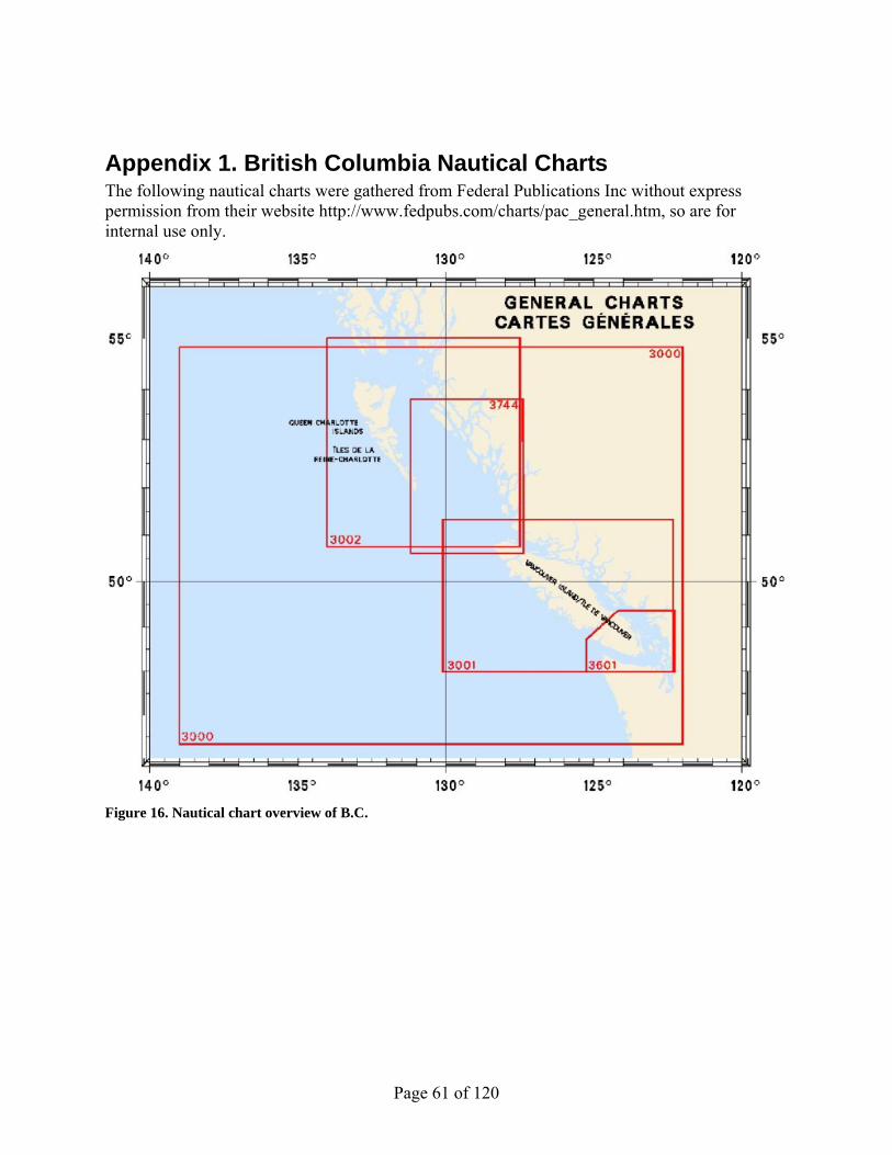
Page 61 of 120
Appendix 1. British Columbia Nautical Charts The following nautical charts were gathered from Federal Publications Inc without express permission from their website http://www.fedpubs.com/charts/pac_general.htm, so are for internal use only.
Figure 16. Nautical chart overview of B.C.

Page 62 of 120
Figure 17. Nautical chart for North Coast of B.C.

Page 63 of 120
Figure 18. Nautical chart for South Coast of B.C.

Page 64 of 120
Figure 19. Nautical chart for Large Scale North B.C.
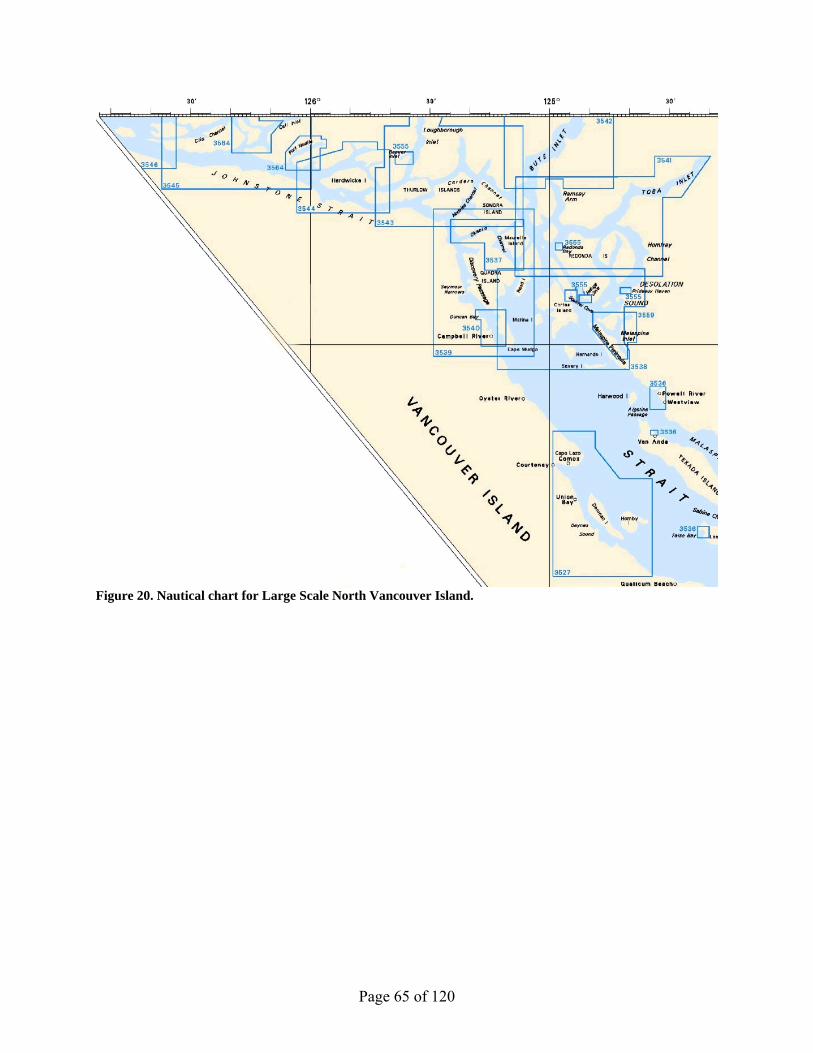
Page 65 of 120
Figure 20. Nautical chart for Large Scale North Vancouver Island.

Page 66 of 120
Figure 21. Nautical chart for Large Scale South Vancouver Island.

Page 67 of 120
Figure 22. Nautical chart for the Queen Charlotte Islands.

Page 68 of 120
Appendix 2. Maps of Observations
Harbour porpoise
Figure 23. Observations of harbour porpoise by group size for all surveys (2004-2008), after truncating perpendicular distance (w) to within 600m.

Page 69 of 120
Dall’s porpoise
Figure 24. Observations of Dall’s porpoise by group size for all surveys (2004-2008), after truncating perpendicular distance (w) to within 700m.

Page 70 of 120
Pacific white-sided dolphin
Figure 25. Observations of Pacific white-sided dolphin by group size for all surveys (2004-2008), after truncating perpendicular distance (w) to within 1200m.

Page 71 of 120
Humpback whale
Figure 26. Observations of humpback whale by group size for all surveys (2004-2008), after truncating perpendicular distance (w) to within 2300m.

Page 72 of 120
Fin whale
Figure 27. Observations of fin whale by group size for all surveys (2004-2008), after truncating perpendicular distance (w) to within 3900m.
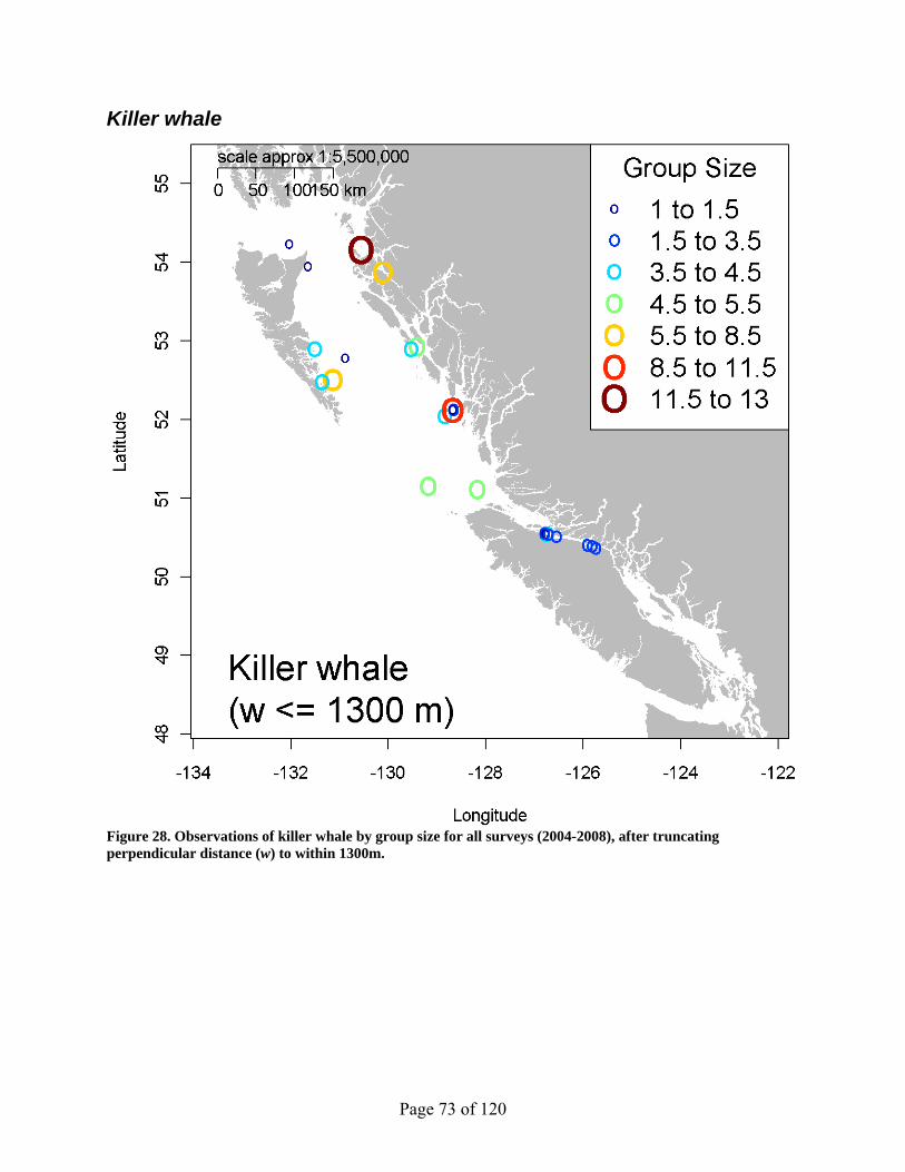
Page 73 of 120
Killer whale
Figure 28. Observations of killer whale by group size for all surveys (2004-2008), after truncating perpendicular distance (w) to within 1300m.

Page 74 of 120
Minke whale
Figure 29. Observations of minke whale by group size for all surveys (2004-2008), after truncating perpendicular distance (w) to within 400m.

Page 75 of 120
Harbour seal, haul-out
Figure 30. Observations of harbour seal, haul-out, by group size for all surveys (2004-2008), after truncating perpendicular distance (w) to within 700m.

Page 76 of 120
Harbour seal, in-water
Figure 31. Observations of harbour seal, in-water, by group size for all surveys (2004-2008), after truncating perpendicular distance (w) to within 500m.

Page 77 of 120
Stellar sea lion, haul-out
Figure 32. Observations of Steller sea lion, haul-out, by group size for all surveys (2004-2008), after truncating perpendicular distance (w) to within 1300m.

Page 78 of 120
Steller sea lion, in-water
Figure 33. Observations of Steller sea lion, in-water, by group size for all surveys (2004-2008), after truncating perpendicular distance (w) to within 500m.

Page 79 of 120
Elephant seal
Figure 34. Observations of elephant seal, haul-out, by group size for all surveys (2004-2008), after truncating perpendicular distance (w) to within 500m.

Page 80 of 120
Appendix 3. Maps of Environmental Covariates
Depth
Figure 35. Static covariate bathymetric depth at 5km grid resolution in meters.

Page 81 of 120
Slope
Figure 36. Static covariate slope derived from bathymetric depth in percent degrees at 5km grid resolution.

Page 82 of 120
Distance to Coast
Figure 37. Static covariate distance to coast (distcoast) in meters at 5km grid resolution.

Page 83 of 120
Dynamic Variables: SST, Chl
Figure 38. Dynamic predictor variables sea-surface temperature (sst) in degrees Celsius and chlorophyll (chl) in mg/m3 given for July, 2008 and averaged over the summer months.

Page 84 of 120
Appendix 4. Density Surface Model Outputs
Harbour Porpoise
Figure 39. Density surface model of harbour porpoise, in # of individuals per square kilometer.

Page 85 of 120
Figure 40. Standard error for density surface of harbour porpoise.

Page 86 of 120
Figure 41. GAM predictor terms for density surface model of harbour porpoise. What is the purpose of these figures- need to be discussed.

Page 87 of 120
Dall’s porpoise
Figure 42. Density surface model of Dall’s porpoise, in # of individuals per square kilometer.

Page 88 of 120
Figure 43. Standard error for distribution model of Dall's porpoise.

Page 89 of 120
Figure 44. GAM terms plot for density surface model of Dall’s porpoise.

Page 90 of 120
Pacific white-sided dolphin
Figure 45. Density surface model of Pacfic white-sided dolphin, in # of individuals per square kilometer.

Page 91 of 120
Figure 46. Standard error for density surface model of Pacific white-sided dolphin.

Page 92 of 120
Figure 47. GAM terms plot for density surface model of Pacific white-sided dolphin.

Page 93 of 120
Humpback whale
Figure 48. Density surface model for humpback whale, in # of individuals per square kilometer.

Page 94 of 120
Figure 49. Standard error for density surface model of humpback whale.

Page 95 of 120
Figure 50. GAM terms plot for humpback whale density surface model in stratum 1.

Page 96 of 120
Figure 51. GAM terms plot for humpback whale density surface model in strata 2,3,4.

Page 97 of 120
Fin whale
Figure 52. Density surface model for fin whale, in # of individuals per square kilometer.

Page 98 of 120
Figure 53. Standard error for density surface model of fin whale.

Page 99 of 120
Figure 54. GAM terms plot for density surface model of fin whale.

Page 100 of 120
Killer whale
Figure 55. Density surface model of killer whale, in # of individuals per square kilometer.

Page 101 of 120
Figure 56. Standard error for density surface model of killer whale.

Page 102 of 120
Figure 57. GAM terms plot for density surface of killer whale.

Page 103 of 120
Minke whale
Figure 58. Density surface model for minke whale, in # of individuals per square kilometer.

Page 104 of 120
Figure 59. Standard error for density surface model of minke whale.

Page 105 of 120
Figure 60. GAM terms plot for density surface model of minke whale.

Page 106 of 120
Harbour seal, haul-out
Figure 61. Density surface model of harbour seal, haul-out, in # of individuals per square kilometer.

Page 107 of 120
Figure 62. Standard error for density surface model of harbour seal, haul-out.

Page 108 of 120
Figure 63. GAM terms plot for density surface model of harbour seal, haul-out.

Page 109 of 120
Harbour seal, in-water
Figure 64. Density surface model for harbour seal, in-water, in # of individuals per square kilometer.

Page 110 of 120
Figure 65. Standard error for density surface model for harbour seal, in-water.

Page 111 of 120
Figure 66. GAM term plots for density surface model for harbour seal, in-water.
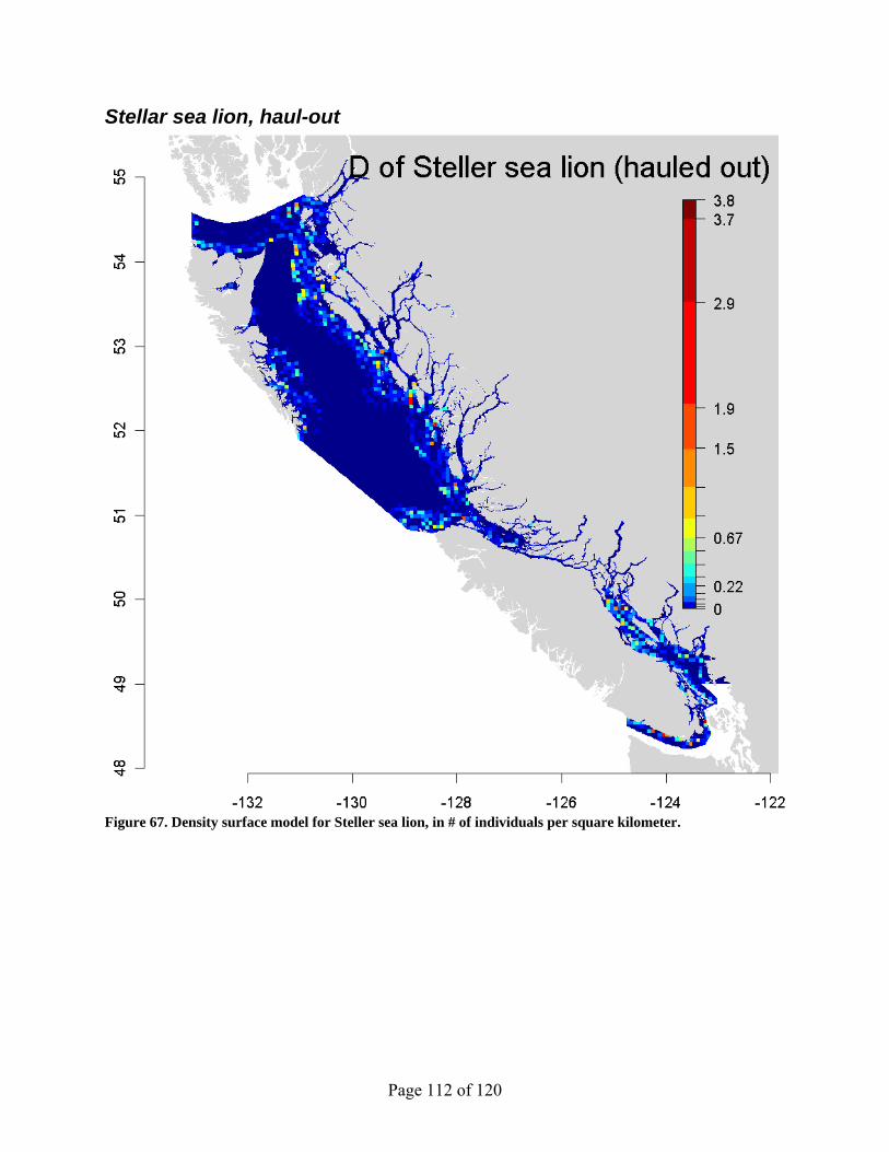
Page 112 of 120
Stellar sea lion, haul-out
Figure 67. Density surface model for Steller sea lion, in # of individuals per square kilometer.

Page 113 of 120
Figure 68. Standard error for density surface model of steller sea lion, haul-out.

Page 114 of 120
Figure 69. GAM terms plot for density surface model of Steller sea lion, haul-out.

Page 115 of 120
Steller sea lion, in-water
Figure 70. Density surface for Steller sea lion, in-water, in # of individuals per square kilometer.

Page 116 of 120
Figure 71. Standard error for density surface model of Steller sea lion.

Page 117 of 120
Figure 72. GAM terms plot for density surface model of Steller sea lion, in-water.

Page 118 of 120
Elephant seal
Figure 73. Density surface for elephant seal, in # of individuals per square kilometer.
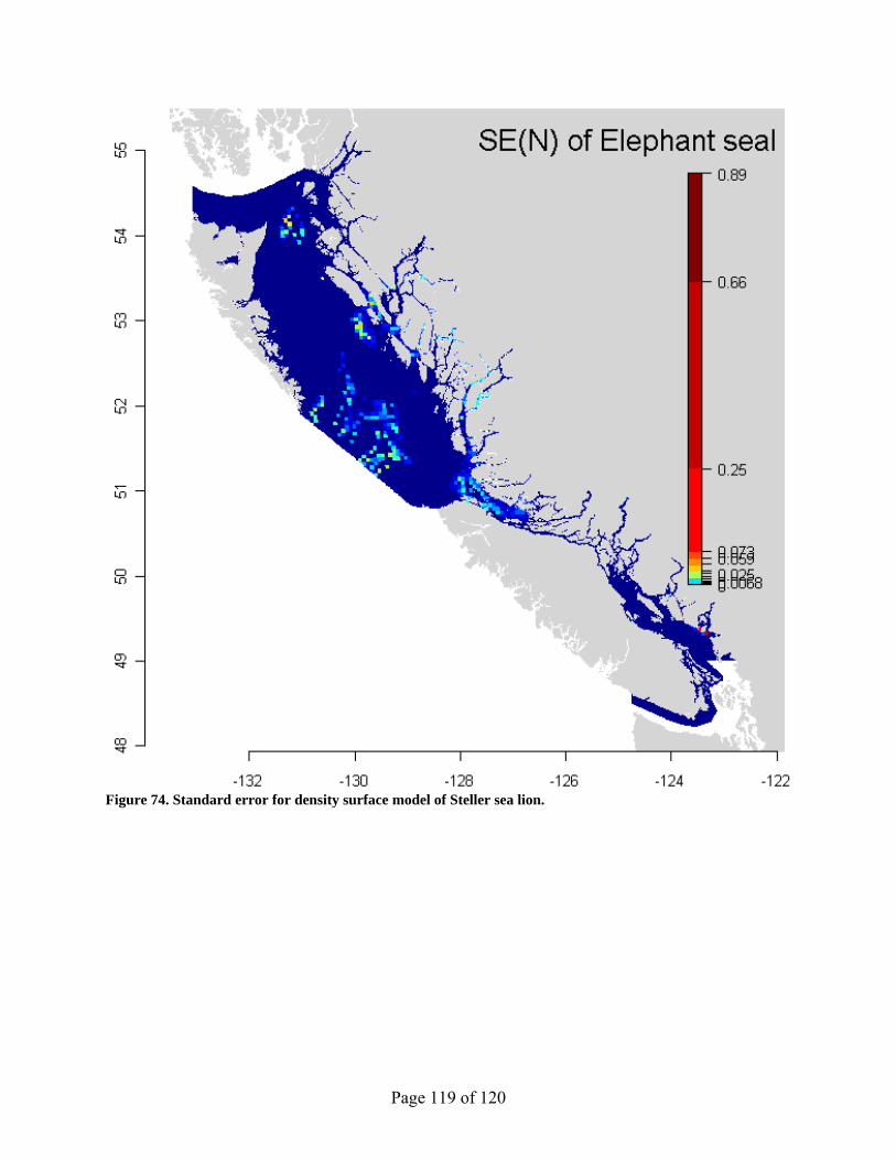
Page 119 of 120
Figure 74. Standard error for density surface model of Steller sea lion.

Page 120 of 120
Figure 75. GAM terms plot for density surface model of elephant seal.