predictive analytics using sas

1

Can Predictive Analytics Be Used to Determine What Led to

the Golden State Warriors Defeat in the 2016 NBA Finals?

Multiple Regression Analysis and Data Visualizations Presented in SAS

Author: Ed Orlando

University: Valparaiso University

Course: Introduction to SAS

Assignment: Capstone Project

Professor: Dr. Hui Gong

2

Table of Contents Introduction……………………………………………………………………………………………………………………………………………………………………………… 4 National Basketball Association (NBA) Data Utilized and Explained…………………………………………………………………………………………….. 4 Summary Statistics…………………………………………………………………………………………………………………………………………………………………….. 4 Summary of Mean Statistics Listed Above…………………………………………………………………………………………………………………………………… 5 Initial Scatterplots of the Independent Variables Versus the Dependent Variable…………………………………………………………………………. 5 Initial Multiple Regression Model 01…………………………………………………………………………………………………………………………………………... 10 Multiple Regression Model 02…………………………………………………………………………………………………………………………………………………..... 11 Tests for Normality……………………………………………………………………………………………………………………………………………………………………. 13 Data Transformation – Defensive Rebounds Variable………………………………………………………………………………………………………………….. 15 Multiple Regression Model 03……………………………………………………………………………………………………………………………………………………. 16 Accuracy & Predictability of Model…………………………………………………………………………………………………………………………………………….. 17 References………………………………………………………………………………………………………………………………………………………………………………… 18 Appendix…………………………………………………………………………………………………………………………………………………………………………………… 19

Tables Table 1: Variable Names and Descriptions…………………………………………………………………………………………………………………………………… 4 Table 2: Summary Statistics for the Golden State Warriors 2015-2016 Season………………………………………………………………………………. 5 Table 3: Aggregated Mean Variances, Expected Sign versus Actual Sign………………………………………………………………………………………… 5 Table 4: Number of Observations Read for Multiple Regression Model 01…………………………………………………………………………………….. 10 Table 5: ANOVA table results for Multiple Regression Model 01……………………………………………………………………………………………………. 10 Table 6: Parameter Estimates for Initial Regression Model 01………………………………………………………………………………………………………. 10 Table 7: Number of Observations Read for Multiple Regression Model 02…………………………………………………………………………………….. 11 Table 8: ANOVA table results for Multiple Regression Model 02……………………………………………………………………………………………………. 11 Table 9: Parameter Estimates for Regression Model 02………………………………………………………………………………………………………………… 11 Table 10: Field Goal Percentage Tests for Normality Output…………………………………………………………………………………………………………. 13 Table 11: Three Point Percentage Tests for Normality Output………………………………………………………………………………………………………. 13 Table 12: Free Throw Percentage Tests for Normality Output………………………………………………………………………………………………………. 14 Table 13: Defensive Rebound Tests for Normality Output (Before Transformation)……………………………………………………………………… 15 Table 14: Defensive Rebound Tests for Normality Output (After Transformation)………………………………………………………………………… 15 Table 15: Number of Observations Read for Multiple Regression Model 03…………………………………………………………………………………… 16 Table 16: ANOVA table results for Multiple Regression Model 03…………………………………………………………………………………………………. 16 Table 17: Parameter Estimates for Regression Model 03……………………………………………………………………………………………………………… 17 Table 18: NBA Final Predictions Based off Multiple Regression Model versus Actual Results…………………………………………………………. 17

3

Graphs Graph 1: Regression Line and Scatterplot for Point Total Variance versus Field Goal Attempt Variance………………………………………… 6 Graph 2: Regression Line and Scatterplot for Point Total Variance versus Field Goal % Variance………………………………………………….. 6 Graph 3: Regression Line and Scatterplot for Point Total Variance versus Three Point % Variance……………………………………………….. 6 Graph 4: Regression Line and Scatterplot for Point Total Variance versus Free Throw Attempt Variance……………………………………… 7 Graph 5: Regression Line and Scatterplot for Point Total Variance versus Free Throw Attempt Variance……………………………………… 7 Graph 6: Regression Line and Scatterplot for Point Total Variance versus Offensive Rebound Variance………………………………………… 7 Graph 7: Regression Line and Scatterplot for Point Total Variance versus Defensive Rebound Variance………………………………………… 8 Graph 8: Regression Line and Scatterplot for Point Total Variance versus Assists Variance………………………………………………………….... 8 Graph 9: Regression Line and Scatterplot for Point Total Variance versus Turnover Variance……………………………………………………….. 8 Graph 10: Regression Line and Scatterplot for Point Total Variance versus Steal Variance……………………………………………………………. 9 Graph 11: Regression Line and Scatterplot for Point Total Variance versus Blocks Variance…………………………………………………………. 9 Graph 12: Regression Line and Scatterplot for Point Total Variance versus Personal Fouls Variance…………………………………………….. 9 Graph 13: Fit Diagnostic for Points and Residual by Regressors for Points……………………………………………………………………………………. 12 Graph 14: Histogram Distribution for Field Goal Percentage………………………………………………………………………………………………………… 13 Graph 15: Histogram Distribution for Three Point Percentage……………………………………………………………………………………………………... 14 Graph 16: Histogram Distribution for Free Throw Percentage……………………………………………………………………………………………………… 14 Graph 17: Histogram Distribution for Defensive Rebounds (Before Transformation)……………………………………………………………………. 15 Graph 18: Histogram Distribution for Defensive Rebounds (After Transformation)………………………………………………………………………. 16

4

Introduction: The Golden State Warriors accomplished something that no other NBA team accomplished during the regular season. The Warriors won a record-beating 73 games in 2016 and only incurred 9 loses during that same time frame. The Warriors beat the record of one of the most decorated and considered by most experts one of the greatest teams of all-time, the 1995-1996 Chicago Bulls. The Chicago Bulls held a record of 72-10 (72 wins / 10 losses) that year and went on to win the NBA finals. Although the Warriors beat the all-time regular season record, they fell one game short of winning the NBA Finals when they lost to Lebron James and the Cleveland Cavaliers. This study will try to determine any of the significant factors that contributed to the Golden State Warriors loss during the NBA finals.

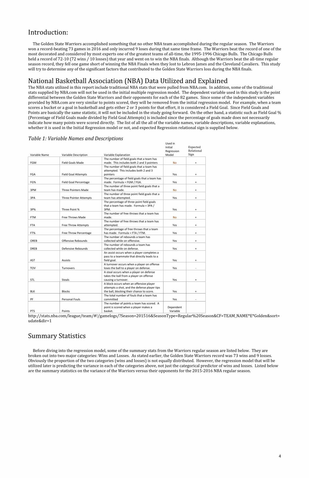
National Basketball Association (NBA) Data Utilized and Explained The NBA stats utilized in this report include traditional NBA stats that were pulled from NBA.com. In addition, some of the traditional stats supplied by NBA.com will not be used in the initial multiple regression model. The dependent variable used in this study is the point differential between the Golden State Warriors and their opponents for each of the 82 games. Since some of the independent variables provided by NBA.com are very similar to points scored, they will be removed from the initial regression model. For example, when a team scores a bucket or a goal in basketball and gets either 2 or 3 points for that effort, it is considered a Field Goal. Since Field Goals and Points are basically the same statistic, it will not be included in the study going forward. On the other hand, a statistic such as Field Goal % (Percentage of Field Goals made divided by Field Goal Attempts) is included since the percentage of goals made does not necessarily indicate how many points were scored directly. The list of all the all of the variable names, variable descriptions, variable explanations, whether it is used in the Initial Regression model or not, and expected Regression relational sign is supplied below. Table 1: Variable Names and Descriptions

Variable Name Variable Description Variable Explanation

Used in Initial Regression Model

Expected Relational Sign

FGM Field Goals Made The number of field goals that a team has made. This includes both 2 and 3 pointers No +

FGA Field Goal Attempts

The number of field goals that a team has attempted. This includes both 2 and 3 pointers Yes +

FG% Field Goal Percentage The percentage of field goals that a team has made. Formula = FGM / FGA. Yes +

3PM Three Pointers Made The number of three point field goals that a team has made. No +

3PA Three Pointer Attempts The number of three point field goals that a team has attempted. Yes +

3P% Three Point %

The percentage of three point field goals that a team has made. Formula = 3PA / 3PM. Yes +

FTM Free Throws Made The number of free throws that a team has made. No +

FTA Free Throw Attempts The number of free throws that a team has attempted. Yes +

FT% Free Throw Percentage The percentage of free throws that a team has made. Formula = FTA / FTM. Yes +

OREB Offensive Rebounds The number of rebounds a team has collected while on offensive. Yes +

DREB Defensive Rebounds The number of rebounds a team has collected while on defense. Yes +

AST Assists

An assist occurs when a player completes a pass to a teammate that directly leads to a field goal. Yes +

TOV Turnovers A turnover occurs when a player on offense loses the ball to a player on defense. Yes -

STL Steals

A steal occurs when a player on defense takes the ball from a player on offense causing a turnover. Yes +

BLK Blocks

A block occurs when an offensive player attempts a shot, and the defense player tips the ball, blocking their chance to score.

Yes

+

PF Personal Fouls The total number of fouls that a team has committed

Yes

-

PTS Points

The number of points a team has scored. A point is scored when a player makes a basket.

Dependent

Variable

http://stats.nba.com/league/team/#!/gamelogs/?Season=201516&SeasonType=Regular%20Season&CF=TEAM_NAME*E*Golden&sort=udate&dir=1

Summary Statistics Before diving into the regression model, some of the summary stats from the Warriors regular season are listed below. They are broken out into two major categories: Wins and Losses. As stated earlier, the Golden State Warriors record was 73 wins and 9 losses. Obviously the proportion of the two categories (wins and losses) is not equally distributed. However, the regression model that will be utilized later is predicting the variance in each of the categories above, not just the categorical predictor of wins and losses. Listed below are the summary statistics on the variance of the Warriors versus their opponents for the 2015-2016 NBA regular season.

5

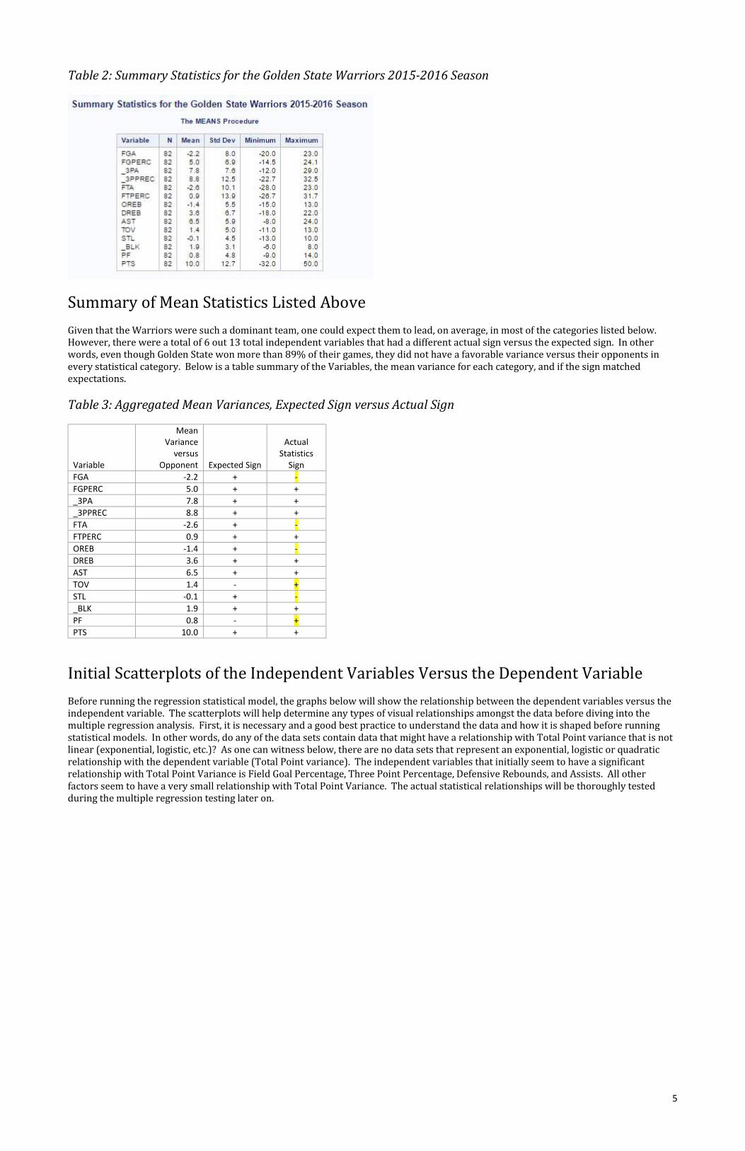
Table 2: Summary Statistics for the Golden State Warriors 2015-2016 Season

Summary of Mean Statistics Listed Above Given that the Warriors were such a dominant team, one could expect them to lead, on average, in most of the categories listed below. However, there were a total of 6 out 13 total independent variables that had a different actual sign versus the expected sign. In other words, even though Golden State won more than 89% of their games, they did not have a favorable variance versus their opponents in every statistical category. Below is a table summary of the Variables, the mean variance for each category, and if the sign matched expectations. Table 3: Aggregated Mean Variances, Expected Sign versus Actual Sign

Variable

Mean Variance

versus Opponent

Expected Sign

Actual

Statistics Sign

FGA -2.2 + - FGPERC 5.0 + + _3PA 7.8 + + _3PPREC 8.8 + + FTA -2.6 + - FTPERC 0.9 + + OREB -1.4 + - DREB 3.6 + + AST 6.5 + + TOV 1.4 - + STL -0.1 + - _BLK 1.9 + + PF 0.8 - + PTS 10.0 + +

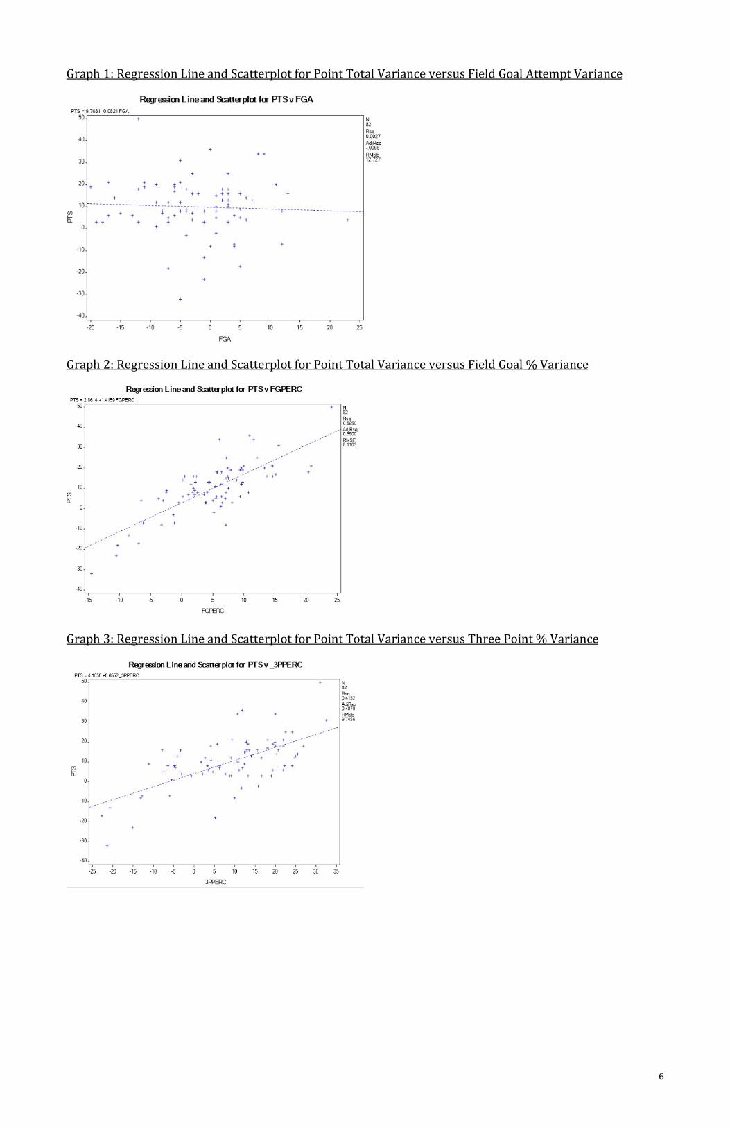
Initial Scatterplots of the Independent Variables Versus the Dependent Variable Before running the regression statistical model, the graphs below will show the relationship between the dependent variables versus the independent variable. The scatterplots will help determine any types of visual relationships amongst the data before diving into the multiple regression analysis. First, it is necessary and a good best practice to understand the data and how it is shaped before running statistical models. In other words, do any of the data sets contain data that might have a relationship with Total Point variance that is not linear (exponential, logistic, etc.)? As one can witness below, there are no data sets that represent an exponential, logistic or quadratic relationship with the dependent variable (Total Point variance). The independent variables that initially seem to have a significant relationship with Total Point Variance is Field Goal Percentage, Three Point Percentage, Defensive Rebounds, and Assists. All other factors seem to have a very small relationship with Total Point Variance. The actual statistical relationships will be thoroughly tested during the multiple regression testing later on.

6

Graph 1: Regression Line and Scatterplot for Point Total Variance versus Field Goal Attempt Variance

Graph 2: Regression Line and Scatterplot for Point Total Variance versus Field Goal % Variance

Graph 3: Regression Line and Scatterplot for Point Total Variance versus Three Point % Variance

7

Graph 4: Regression Line and Scatterplot for Point Total Variance versus Free Throw Attempt Variance

Graph 5: Regression Line and Scatterplot for Point Total Variance versus Free Throw Attempt Variance

Graph 6: Regression Line and Scatterplot for Point Total Variance versus Offensive Rebound Variance

8

Graph 7: Regression Line and Scatterplot for Point Total Variance versus Defensive Rebound Variance

Graph 8: Regression Line and Scatterplot for Point Total Variance versus Assists Variance

Graph 9: Regression Line and Scatterplot for Point Total Variance versus Turnover Variance

9

Graph 10: Regression Line and Scatterplot for Point Total Variance versus Steal Variance

Graph 11: Regression Line and Scatterplot for Point Total Variance versus Blocks Variance

Graph 12: Regression Line and Scatterplot for Point Total Variance versus Personal Fouls Variance

10

Initial Multiple Regression Model 01 Even though some of the independent variables do not seem to have a strong relationship with Total Point Variance, all of the variables will be used in the initial regression model. After the model is ran, it will then be determined which variables will be eliminated from being used in some of the additional tests that will be performed. Listed below is the multiple regression results. Table 4: Number of Observations Read for Multiple Regression Model 01

Number of Observations Read 82

Number of Observations Used 82

Eighty -two games were played in the regular season for the Golden State Warriors.

Table 5: ANOVA table results for Multiple Regression Model 01

Analysis of Variance

Source DF Sum of

Squares Mean

Square F

Value Pr > F

Model 13 12,705 977.32 230.28 <.0001

Error 68 288.60 4.24

Corrected Total 81 12,994

Root MSE 2.06 R-Square 0.9778

Dependent Mean 9.95 Adj R-Sq 0.9735

Coeff Var 20.70

The p-value of the entire model is significant at p-value < 0.05 and had an adjusted R-Square value of 0.9735.

The model is probably overfed meaning that the Adjusted R-Square value is too large at 0.9735. In other words, the independent variables that we have included match very closely with the total point variance. The model most likely has too many variables that are too closely related with the total point variance and the future model. However, at this point, the Parameter Estimates graph listed below highlight the variables that have a significant relationship with the Total Point Variance Variable. Therefore, OREB, AST, TOV, STL, _BLK, and PF (see Table 1 for explanation of variables) can be removed from the model. In addition, FGA (Field Goals Attempts), _3PA (Three Point Attempts), & FTA (Free Throw Attempts) will be removed from the next model.

When one combines, Field Goal attempts (how many shots the team took) and Field Goal Percentage, the multiplication of the two variables ultimately calculates how many points the team scored, which can be contributing to the overfitting. Likewise, the same statement can be made with Three Point Field Goal % and Three Point attempts as well as Free Throw % and Free Throw attempts.

Table 6: Parameter Estimates for Initial Regression Model 01

Parameter Estimates

Variable DF Parameter

Estimate Standard

Error t Value Pr > |t|

Intercept 1 -0.17029 0.44124 -0.39 0.7008

FGA 1 0.77230 0.08380 9.22 <.0001

FGPERC 1 1.64524 0.08013 20.53 <.0001

_3PA 1 0.31638 0.03330 9.50 <.0001

_3PPERC 1 0.23734 0.02800 8.47 <.0001

FTA 1 0.68081 0.05433 12.53 <.0001

FTPERC 1 0.21503 0.02040 10.54 <.0001

OREB 1 0.02503 0.09973 0.25 0.8026

DREB 1 0.15142 0.07744 1.96 0.0547

AST 1 0.05368 0.05280 1.02 0.3129

TOV 1 -0.10787 0.09730 -1.11 0.2715

STL 1 0.03281 0.07107 0.46 0.6458

_BLK 1 -0.04483 0.08702 -0.52 0.6081

PF 1 0.05185 0.08807 0.59 0.5580

At this point, for this model, none of the other output statistics are included since the model is most likely overfed. This initial model was primarily used to find significant values that can be potentially carried over into the simpler Regression models presented later in this paper.

11

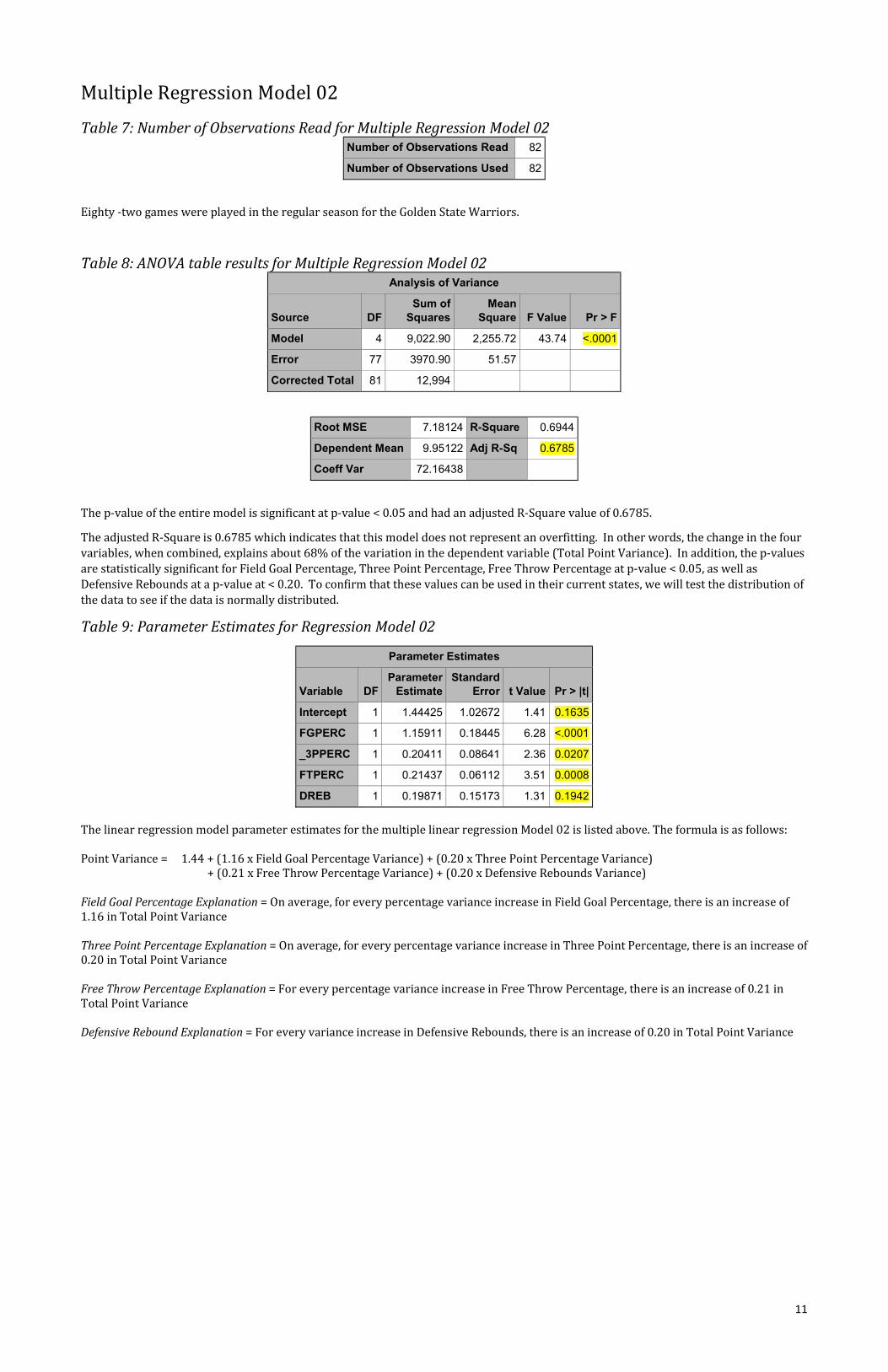
Multiple Regression Model 02 Table 7: Number of Observations Read for Multiple Regression Model 02



Eighty -two games were played in the regular season for the Golden State Warriors.

Table 8: ANOVA table results for Multiple Regression Model 02 Analysis of Variance

Source DF Sum of

Squares Mean

Square F Value Pr > F

Model 4 9,022.90 2,255.72 43.74 <.0001

Error 77 3970.90 51.57




Coeff Var 72.16438


The adjusted R-Square is 0.6785 which indicates that this model does not represent an overfitting. In other words, the change in the four variables, when combined, explains about 68% of the variation in the dependent variable (Total Point Variance). In addition, the p-values are statistically significant for Field Goal Percentage, Three Point Percentage, Free Throw Percentage at p-value < 0.05, as well as Defensive Rebounds at a p-value at < 0.20. To confirm that these values can be used in their current states, we will test the distribution of the data to see if the data is normally distributed.

Table 9: Parameter Estimates for Regression Model 02

Parameter Estimates


Estimate Standard


Intercept 1 1.44425 1.02672 1.41 0.1635

FGPERC 1 1.15911 0.18445 6.28 <.0001

_3PPERC 1 0.20411 0.08641 2.36 0.0207

FTPERC 1 0.21437 0.06112 3.51 0.0008

DREB 1 0.19871 0.15173 1.31 0.1942

The linear regression model parameter estimates for the multiple linear regression Model 02 is listed above. The formula is as follows: Point Variance = 1.44 + (1.16 x Field Goal Percentage Variance) + (0.20 x Three Point Percentage Variance)

+ (0.21 x Free Throw Percentage Variance) + (0.20 x Defensive Rebounds Variance) Field Goal Percentage Explanation = On average, for every percentage variance increase in Field Goal Percentage, there is an increase of 1.16 in Total Point Variance Three Point Percentage Explanation = On average, for every percentage variance increase in Three Point Percentage, there is an increase of 0.20 in Total Point Variance Free Throw Percentage Explanation = For every percentage variance increase in Free Throw Percentage, there is an increase of 0.21 in Total Point Variance Defensive Rebound Explanation = For every variance increase in Defensive Rebounds, there is an increase of 0.20 in Total Point Variance

12

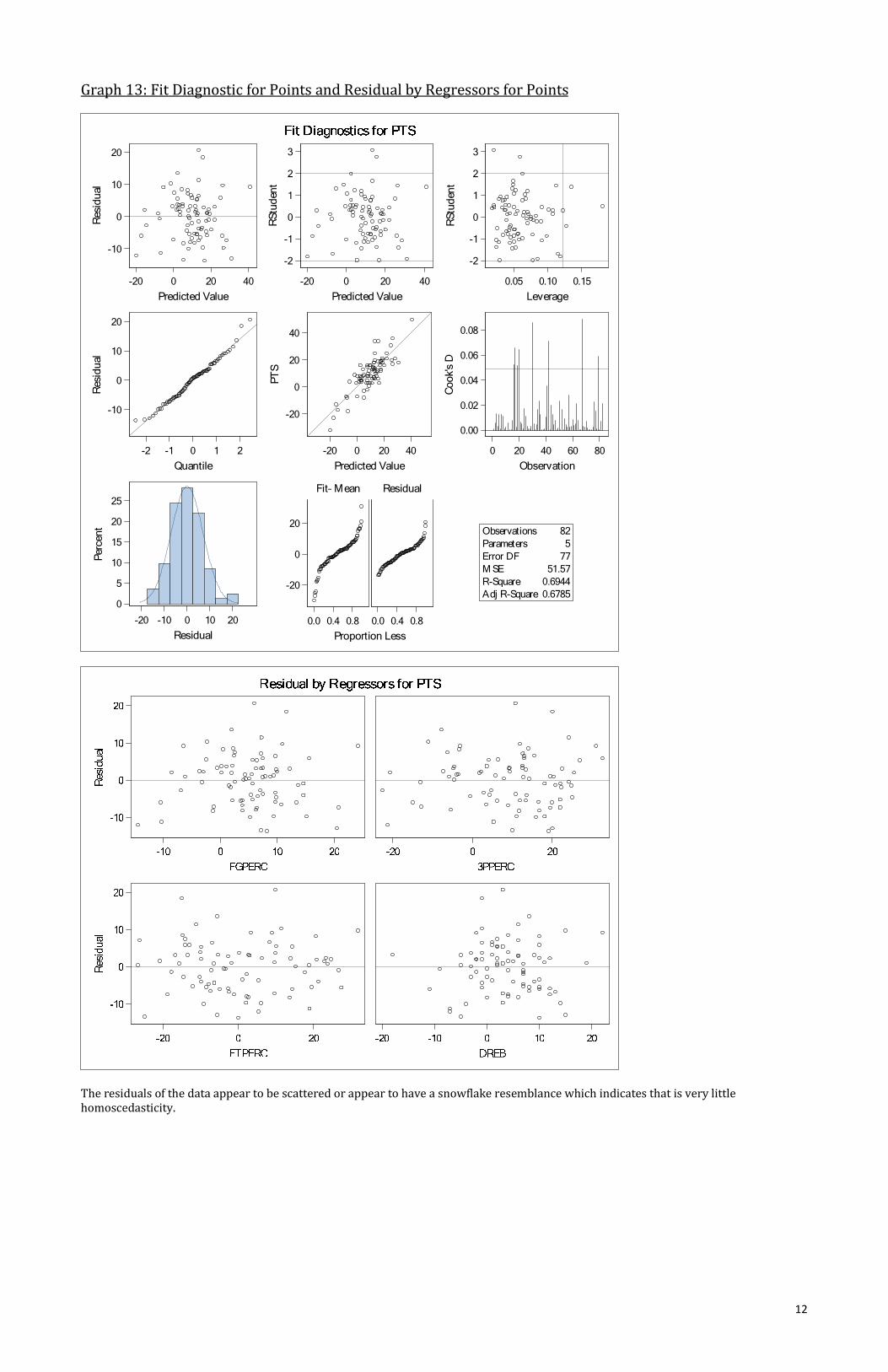
Graph 13: Fit Diagnostic for Points and Residual by Regressors for Points

The residuals of the data appear to be scattered or appear to have a snowflake resemblance which indicates that is very little homoscedasticity.

0.6785Adj R-Square0.6944R-Square51.57M SE

77Error DF5Parameters

82Observations

Proportion Less0.0 0.4 0.8

Residual

0.0 0.4 0.8

Fit– Mean

-20

0

20

-20 -10 0 10 20

Residual

0

5

10

15

20

25

Perc

ent

0 20 40 60 80

Observation

0.00

0.02

0.04

0.06

0.08

Coo

k's

D-20 0 20 40

Predicted Value

-20

0

20

40

PTS

-2 -1 0 1 2

Quantile

-10

0

10

20

Res

idua

l

0.05 0.10 0.15

Leverage

-2

-1

0

1

2

3

RSt

uden

t

-20 0 20 40

Predicted Value

-2

-1

0

1

2

3

RSt

uden

t-20 0 20 40

Predicted Value

-10

0

10

20

Res

idua

l

13

Tests for Normality One last test to ensure that the variables above should be utilized in the multiple regression model in their current state is to test to see if the independent variables are normally distributed. Listed below are the histogram and normal distribution tests that were ran in SAS.

Table 10: Field Goal Percentage Tests for Normality Output

Tests for Normality

Test Statistic p Value

Shapiro-Wilk W 0.9801 Pr < W 0.2331

Kolmogorov-Smirnov D 0.0771 Pr > D >0.1500

Cramer-von Mises W-Sq 0.1154 Pr > W-Sq 0.0724

Anderson-Darling A-Sq 0.6689 Pr > A-Sq 0.0817

None of the tests for normality listed above are significant at p-value < 0.05. However, the Cramer-von Mises test and Anderson Darling tests are both significant at p-value = 0.10. Graph 14: Histogram Distribution for Field Goal Percentage

Table 11: Three Point Percentage Tests for Normality Output

Tests for Normality



Kolmogorov-Smirnov D 0.0975 Pr > D 0.0522



Three (3) out of 4 of the tests for normality listed above are significant at p-value < 0.05. In addition, the Kolmogorov-Smirnov test is significant at p-value < 0.10.

Per

cent

14

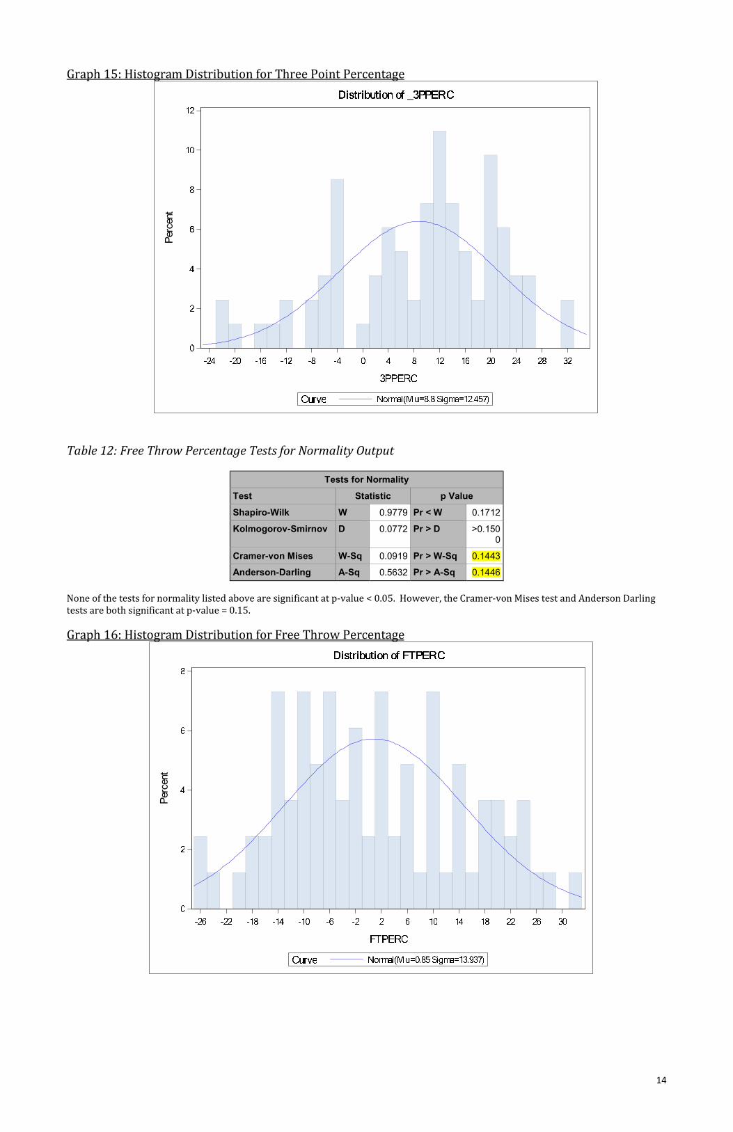
Graph 15: Histogram Distribution for Three Point Percentage

Table 12: Free Throw Percentage Tests for Normality Output

Tests for Normality






None of the tests for normality listed above are significant at p-value < 0.05. However, the Cramer-von Mises test and Anderson Darling tests are both significant at p-value = 0.15.

Graph 16: Histogram Distribution for Free Throw Percentage

Per

cent

Per

cent

15

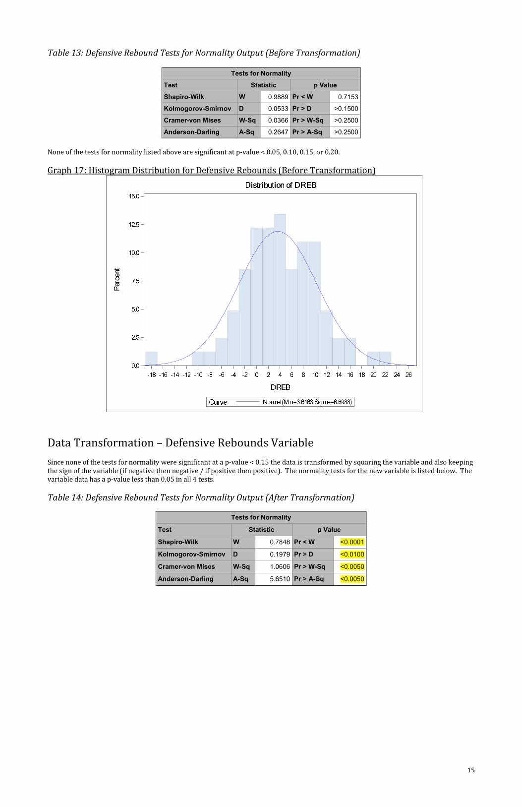
Table 13: Defensive Rebound Tests for Normality Output (Before Transformation)

Tests for Normality




Cramer-von Mises W-Sq 0.0366 Pr > W-Sq >0.2500

Anderson-Darling A-Sq 0.2647 Pr > A-Sq >0.2500

None of the tests for normality listed above are significant at p-value < 0.05, 0.10, 0.15, or 0.20. Graph 17: Histogram Distribution for Defensive Rebounds (Before Transformation)

Data Transformation – Defensive Rebounds Variable Since none of the tests for normality were significant at a p-value < 0.15 the data is transformed by squaring the variable and also keeping the sign of the variable (if negative then negative / if positive then positive). The normality tests for the new variable is listed below. The variable data has a p-value less than 0.05 in all 4 tests. Table 14: Defensive Rebound Tests for Normality Output (After Transformation)

Tests for Normality


Shapiro-Wilk W 0.7848 Pr < W <0.0001

Kolmogorov-Smirnov D 0.1979 Pr > D <0.0100

Cramer-von Mises W-Sq 1.0606 Pr > W-Sq <0.0050

Anderson-Darling A-Sq 5.6510 Pr > A-Sq <0.0050

Per

cent

16

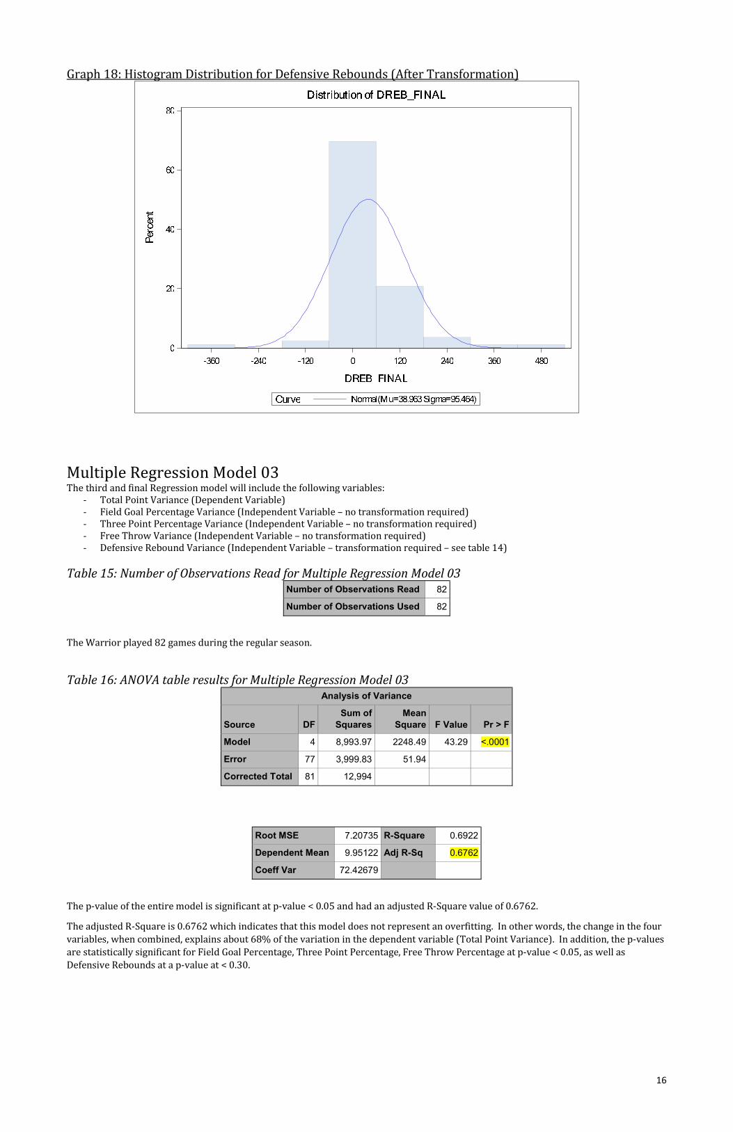
Graph 18: Histogram Distribution for Defensive Rebounds (After Transformation)

Multiple Regression Model 03 The third and final Regression model will include the following variables:

- Total Point Variance (Dependent Variable) - Field Goal Percentage Variance (Independent Variable – no transformation required) - Three Point Percentage Variance (Independent Variable – no transformation required) - Free Throw Variance (Independent Variable – no transformation required) - Defensive Rebound Variance (Independent Variable – transformation required – see table 14)

Table 15: Number of Observations Read for Multiple Regression Model 03



The Warrior played 82 games during the regular season.

Table 16: ANOVA table results for Multiple Regression Model 03

Analysis of Variance

Source DF Sum of

Squares Mean

Square F Value Pr > F

Model 4 8,993.97 2248.49 43.29 <.0001

Error 77 3,999.83 51.94




Coeff Var 72.42679


The adjusted R-Square is 0.6762 which indicates that this model does not represent an overfitting. In other words, the change in the four variables, when combined, explains about 68% of the variation in the dependent variable (Total Point Variance). In addition, the p-values are statistically significant for Field Goal Percentage, Three Point Percentage, Free Throw Percentage at p-value < 0.05, as well as Defensive Rebounds at a p-value at < 0.30.

17

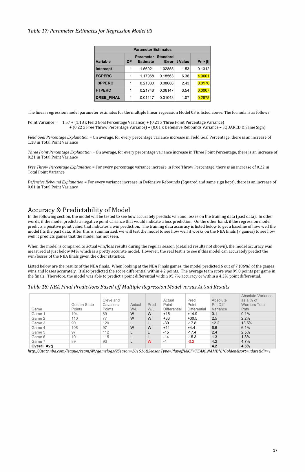
Table 17: Parameter Estimates for Regression Model 03

Parameter Estimates


Estimate Standard


Intercept 1 1.56921 1.02855 1.53 0.1312

FGPERC 1 1.17968 0.18563 6.36 <.0001

_3PPERC 1 0.21080 0.08686 2.43 0.0176

FTPERC 1 0.21746 0.06147 3.54 0.0007

DREB_FINAL 1 0.01117 0.01043 1.07 0.2878

The linear regression model parameter estimates for the multiple linear regression Model 03 is listed above. The formula is as follows: Point Variance = 1.57 + (1.18 x Field Goal Percentage Variance) + (0.21 x Three Point Percentage Variance)

+ (0.22 x Free Throw Percentage Variance) + (0.01 x Defensive Rebounds Variance – SQUARED & Same Sign) Field Goal Percentage Explanation = On average, for every percentage variance increase in Field Goal Percentage, there is an increase of 1.18 in Total Point Variance Three Point Percentage Explanation = On average, for every percentage variance increase in Three Point Percentage, there is an increase of 0.21 in Total Point Variance Free Throw Percentage Explanation = For every percentage variance increase in Free Throw Percentage, there is an increase of 0.22 in Total Point Variance Defensive Rebound Explanation = For every variance increase in Defensive Rebounds (Squared and same sign kept), there is an increase of 0.01 in Total Point Variance

Accuracy & Predictability of Model In the following section, the model will be tested to see how accurately predicts win and losses on the training data (past data). In other words, if the model predicts a negative point variance that would indicate a loss prediction. On the other hand, if the regression model predicts a positive point value, that indicates a win prediction. The training data accuracy is listed below to get a baseline of how well the model fits the past data. After this is summarized, we will test the model to see how well it works on the NBA finals (7 games) to see how well it predicts games that the model has not seen. When the model is compared to actual win/loss results during the regular season (detailed results not shown), the model accuracy was measured at just below 94% which is a pretty accurate model. However, the real test is to see if this model can accurately predict the win/losses of the NBA finals given the other statistics. Listed below are the results of the NBA finals. When looking at the NBA Finals games, the model predicted 6 out of 7 (86%) of the games wins and losses accurately. It also predicted the score differential within 4.2 points. The average team score was 99.8 points per game in the finals. Therefore, the model was able to predict a point differential within 95.7% accuracy or within a 4.3% point differential. Table 18: NBA Final Predictions Based off Multiple Regression Model versus Actual Results

Game

Golden State Points

Cleveland Cavaliers Points

Actual W/L

Pred W/L

Actual Point Differential

Pred Point Differential

Absolute Pnt Diff Variance

Absolute Variance as a % of Warriors Total Pnts

Game 1 104 89 W W +15 +14.9 0.1 0.1% Game 2 110 77 W W +33 +30.5 2.5 2.2% Game 3 90 120 L L -30 -17.8 12.2 13.5% Game 4 108 97 W W +11 +4.4 6.6 6.1% Game 5 97 112 L L -15 -17.4 2.4 2.5% Game 6 101 115 L L -14 -15.3 1.3 1.3% Game 7 89 93 L W -4 -0.2 4.2 4.7% Overall Avg 4.2 4.3%

http://stats.nba.com/league/team/#!/gamelogs/?Season=201516&SeasonType=Playoffs&CF=TEAM_NAME*E*Golden&sort=udate&dir=1

18

References Doane, S. & Seward, L. (2012). Applied statistics in business and economics (4th Ed.). New York, NY: McGraw-Hill/Irwin. Elliott, R. J. & Morrell, C. H. (2010). Learning SAS in the Lab: Third Edition. Boston, MA: Brooks / Cole. League Team Stats. NBA.com. Retrieved on 6/20/16 from

http://stats.nba.com/league/team/#!/gamelogs/?Season=201516&SeasonType=Regular%20Season& CF=TEAM_NAME*E*Golden&sort=udate&dir=1

SAS Certification Prep Guide: Base Programming for SAS 9 Third Edition. Cary, North Carolina: SAS Institute, Inc.

19

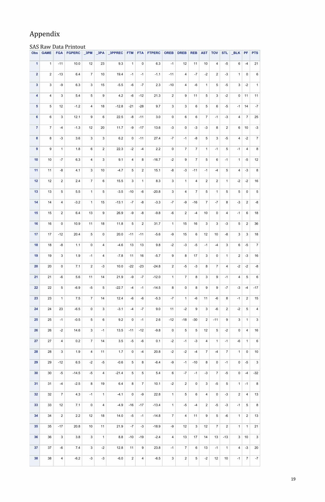
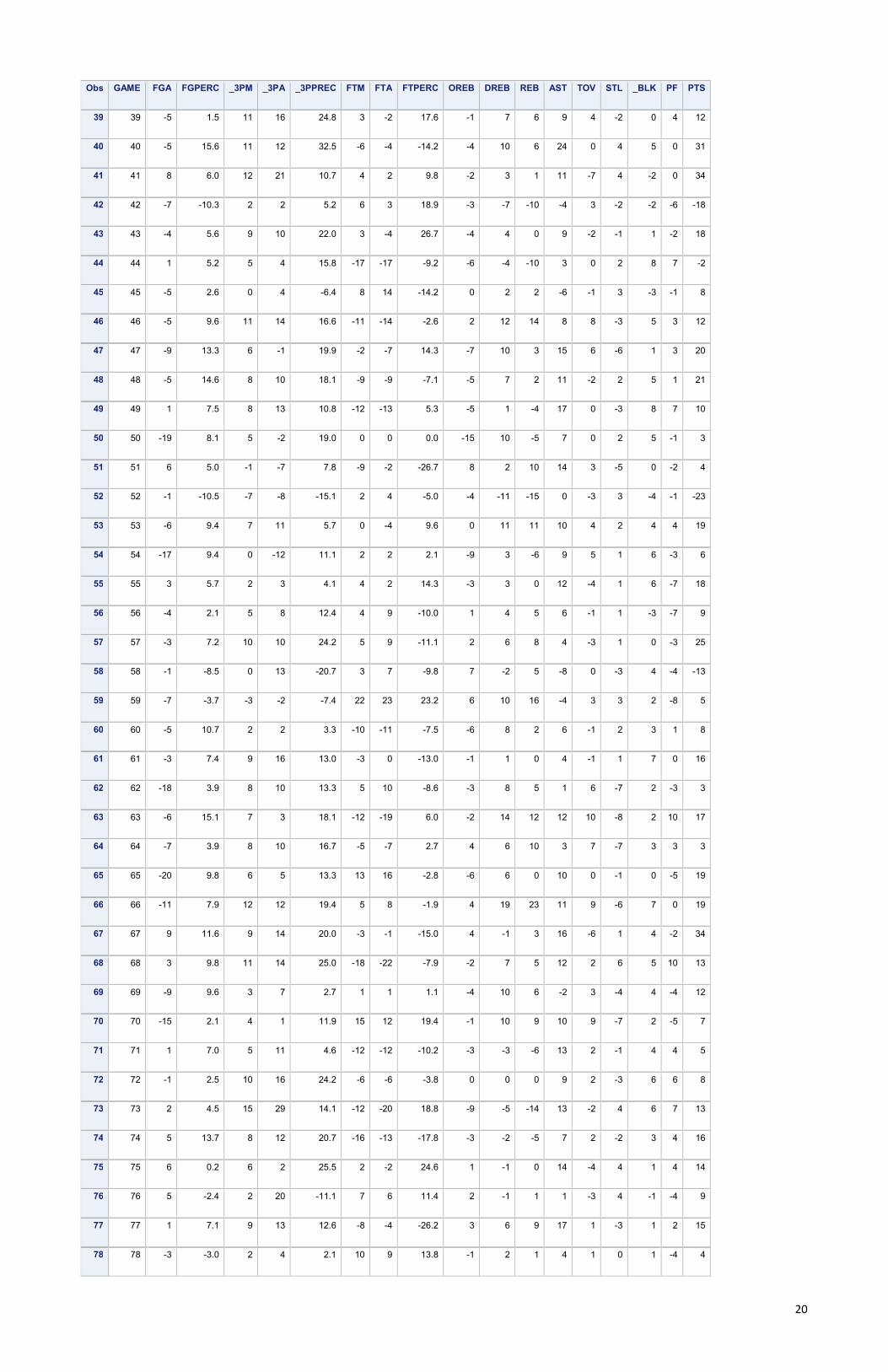
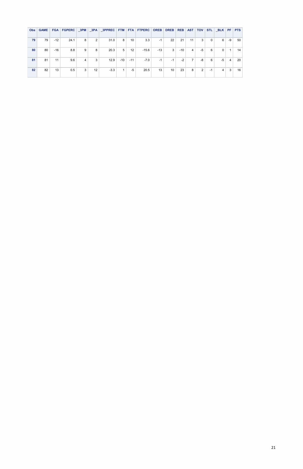
Appendix SAS Raw Data Printout

Obs GAME FGA FGPERC _3PM _3PA _3PPREC FTM FTA FTPERC OREB DREB REB AST TOV STL _BLK PF PTS

1 1 -11 10.0 12 23 9.3 1 0 6.3 -1 12 11 10 4 -5 6 -4 21

2 2 -13 6.4 7 10 19.4 -1 -1 -1.1 -11 4 -7 -2 2 -3 1 0 6

3 3 -9 6.3 3 15 -5.5 -6 -7 2.3 -10 4 -6 1 5 -5 3 -2 1

4 4 3 5.4 5 9 4.2 -6 -12 21.3 2 9 11 5 3 -2 0 11 11

5 5 12 -1.2 4 18 -12.8 -21 -28 9.7 3 3 6 5 6 -5 -1 14 -7

6 6 3 12.1 9 6 22.5 -8 -11 3.0 0 6 6 7 -1 -3 4 7 25

7 7 -4 -1.3 12 20 11.7 -9 -17 13.6 -3 0 -3 -3 8 2 6 10 -3

8 8 -3 3.6 3 3 6.2 0 -11 27.4 -7 -1 -8 5 3 -5 4 -2 7

9 9 1 1.8 6 2 22.3 -2 -4 2.2 0 7 7 1 -1 5 -1 4 8

10 10 -7 6.3 4 3 9.1 4 8 -16.7 -2 9 7 5 6 -1 1 -5 12

11 11 -8 4.1 3 10 -4.7 5 2 15.1 -8 -3 -11 -1 -4 5 4 -3 8

12 12 2 2.4 7 6 15.5 3 1 8.3 3 1 4 2 2 1 -2 -2 16

13 13 5 5.5 1 5 -3.5 -10 -6 -20.8 3 4 7 5 1 5 5 0 5

14 14 4 -3.2 1 15 -13.1 -7 -8 -3.3 -7 -9 -16 7 -7 8 -3 2 -8

15 15 2 6.4 13 9 26.9 -9 -8 -9.8 -6 2 -4 10 0 4 -1 6 18

16 16 0 10.9 11 18 11.8 5 2 31.7 1 15 16 3 3 -3 5 2 36

17 17 -12 20.4 5 0 20.0 -11 -11 -5.6 -9 15 6 12 10 -8 3 3 18

18 18 -8 1.1 0 4 -4.6 13 13 9.8 -2 -3 -5 -1 -4 3 6 -5 7

19 19 3 1.9 -1 4 -7.8 11 16 -5.7 9 8 17 3 0 1 2 -3 16

20 20 0 7.1 2 -3 10.0 -22 -23 -24.8 2 -5 -3 8 7 4 -2 -2 -8

21 21 -6 5.6 11 14 21.9 -9 -7 -12.0 1 7 8 3 9 -1 4 5 6

22 22 5 -6.9 -5 5 -22.7 -4 -1 -14.5 8 0 8 9 9 -7 -3 -4 -17

23 23 1 7.5 7 14 12.4 -6 -6 -5.3 -7 1 -6 11 -6 8 -1 2 15

24 24 23 -6.5 0 3 -3.1 -4 -7 9.0 11 -2 9 3 -6 2 -2 5 4

25 25 -1 -0.5 5 6 9.2 0 -1 2.6 -12 -18 -30 2 -11 9 3 1 3

26 26 -2 14.6 3 -1 13.5 -11 -12 -9.8 0 5 5 12 5 -2 0 4 16

27 27 4 0.2 7 14 3.5 -5 -6 0.1 -2 -1 -3 4 1 -1 -6 1 6

28 28 3 1.9 4 11 1.7 0 -4 20.8 -2 -2 -4 7 -4 7 1 0 10

29 29 -12 6.5 -2 -5 -0.6 5 8 -6.4 -9 -1 -10 8 0 -1 0 -5 3

30 30 -5 -14.5 -5 4 -21.4 5 5 5.4 6 -7 -1 -3 7 -5 0 -4 -32

31 31 -4 -2.5 8 19 6.4 8 7 10.1 -2 2 0 3 -5 5 1 -1 8

32 32 7 4.3 -1 1 -4.1 0 -9 22.8 1 5 6 4 0 -3 2 4 13

33 33 12 7.1 0 4 -4.9 -16 -17 -13.4 1 -5 -4 2 -5 -3 -1 5 8

34 34 2 2.2 12 18 14.0 -5 -1 -14.8 7 4 11 9 5 -6 1 2 13

35 35 -17 20.8 10 11 21.9 -7 -3 -18.9 -9 12 3 12 7 2 1 1 21

36 36 3 3.8 3 1 8.8 -10 -19 -2.4 4 13 17 14 13 -13 3 10 3

37 37 -6 7.4 3 -2 12.8 11 9 23.8 -1 7 6 13 -1 1 4 -3 20

38 38 4 -6.2 -3 -3 -6.0 2 4 -6.5 3 2 5 -2 12 10 -1 7 -7

20


39 39 -5 1.5 11 16 24.8 3 -2 17.6 -1 7 6 9 4 -2 0 4 12

40 40 -5 15.6 11 12 32.5 -6 -4 -14.2 -4 10 6 24 0 4 5 0 31

41 41 8 6.0 12 21 10.7 4 2 9.8 -2 3 1 11 -7 4 -2 0 34

42 42 -7 -10.3 2 2 5.2 6 3 18.9 -3 -7 -10 -4 3 -2 -2 -6 -18

43 43 -4 5.6 9 10 22.0 3 -4 26.7 -4 4 0 9 -2 -1 1 -2 18

44 44 1 5.2 5 4 15.8 -17 -17 -9.2 -6 -4 -10 3 0 2 8 7 -2

45 45 -5 2.6 0 4 -6.4 8 14 -14.2 0 2 2 -6 -1 3 -3 -1 8

46 46 -5 9.6 11 14 16.6 -11 -14 -2.6 2 12 14 8 8 -3 5 3 12

47 47 -9 13.3 6 -1 19.9 -2 -7 14.3 -7 10 3 15 6 -6 1 3 20

48 48 -5 14.6 8 10 18.1 -9 -9 -7.1 -5 7 2 11 -2 2 5 1 21

49 49 1 7.5 8 13 10.8 -12 -13 5.3 -5 1 -4 17 0 -3 8 7 10

50 50 -19 8.1 5 -2 19.0 0 0 0.0 -15 10 -5 7 0 2 5 -1 3

51 51 6 5.0 -1 -7 7.8 -9 -2 -26.7 8 2 10 14 3 -5 0 -2 4

52 52 -1 -10.5 -7 -8 -15.1 2 4 -5.0 -4 -11 -15 0 -3 3 -4 -1 -23

53 53 -6 9.4 7 11 5.7 0 -4 9.6 0 11 11 10 4 2 4 4 19

54 54 -17 9.4 0 -12 11.1 2 2 2.1 -9 3 -6 9 5 1 6 -3 6

55 55 3 5.7 2 3 4.1 4 2 14.3 -3 3 0 12 -4 1 6 -7 18

56 56 -4 2.1 5 8 12.4 4 9 -10.0 1 4 5 6 -1 1 -3 -7 9

57 57 -3 7.2 10 10 24.2 5 9 -11.1 2 6 8 4 -3 1 0 -3 25

58 58 -1 -8.5 0 13 -20.7 3 7 -9.8 7 -2 5 -8 0 -3 4 -4 -13

59 59 -7 -3.7 -3 -2 -7.4 22 23 23.2 6 10 16 -4 3 3 2 -8 5

60 60 -5 10.7 2 2 3.3 -10 -11 -7.5 -6 8 2 6 -1 2 3 1 8

61 61 -3 7.4 9 16 13.0 -3 0 -13.0 -1 1 0 4 -1 1 7 0 16

62 62 -18 3.9 8 10 13.3 5 10 -8.6 -3 8 5 1 6 -7 2 -3 3

63 63 -6 15.1 7 3 18.1 -12 -19 6.0 -2 14 12 12 10 -8 2 10 17

64 64 -7 3.9 8 10 16.7 -5 -7 2.7 4 6 10 3 7 -7 3 3 3

65 65 -20 9.8 6 5 13.3 13 16 -2.8 -6 6 0 10 0 -1 0 -5 19

66 66 -11 7.9 12 12 19.4 5 8 -1.9 4 19 23 11 9 -6 7 0 19

67 67 9 11.6 9 14 20.0 -3 -1 -15.0 4 -1 3 16 -6 1 4 -2 34

68 68 3 9.8 11 14 25.0 -18 -22 -7.9 -2 7 5 12 2 6 5 10 13

69 69 -9 9.6 3 7 2.7 1 1 1.1 -4 10 6 -2 3 -4 4 -4 12

70 70 -15 2.1 4 1 11.9 15 12 19.4 -1 10 9 10 9 -7 2 -5 7

71 71 1 7.0 5 11 4.6 -12 -12 -10.2 -3 -3 -6 13 2 -1 4 4 5

72 72 -1 2.5 10 16 24.2 -6 -6 -3.8 0 0 0 9 2 -3 6 6 8

73 73 2 4.5 15 29 14.1 -12 -20 18.8 -9 -5 -14 13 -2 4 6 7 13

74 74 5 13.7 8 12 20.7 -16 -13 -17.8 -3 -2 -5 7 2 -2 3 4 16

75 75 6 0.2 6 2 25.5 2 -2 24.6 1 -1 0 14 -4 4 1 4 14

76 76 5 -2.4 2 20 -11.1 7 6 11.4 2 -1 1 1 -3 4 -1 -4 9

77 77 1 7.1 9 13 12.6 -8 -4 -26.2 3 6 9 17 1 -3 1 2 15

78 78 -3 -3.0 2 4 2.1 10 9 13.8 -1 2 1 4 1 0 1 -4 4

21


79 79 -12 24.1 8 2 31.0 8 10 3.3 -1 22 21 11 3 0 6 -9 50

80 80 -16 8.8 9 8 20.3 5 12 -15.6 -13 3 -10 4 -5 6 0 1 14

81 81 11 9.6 4 3 12.9 -10 -11 -7.0 -1 -1 -2 7 -8 6 -5 4 20

82 82 13 0.5 3 12 -3.3 1 -5 20.5 13 10 23 8 2 -1 4 3 16

predictive analytics using sas

Documents