Prediction of palm-tree ganoderma affection degree

by reflectance spectroscopy: proposed methodology

Fabrice Dubertret (Internship student in Agriculture Engineering, SupAgro-Montpellier)

& Camille Lelong, PhD. (CIRAD/UMR TETIS Remote-Sensing Researcher)

With the support of Jean-Pierre Caliman, PhD. (CIRAD/UPR 34 – PT-SMART/SMARTRI)

July 2008 – January 2009

Table of Content

Table of Content ...................................................................................................................... iii Introduction .............................................................................................................................. 6 Part A – Context of the study .................................................................................................. 7

I - Framework ......................................................................................................................... 7 I.1 - Welcoming structure ........................................................................................................................ 7 I.2 - Scientific issues ................................................................................................................................ 7 I.3 - PT Smart and Padang Halaban Estate ............................................................................................ 8

II - The cultivated palm-tree ................................................................................................... 9 II.1 - A tropical culture, which became industrial .................................................................................. 9 II.2 - Morphology, Biology and cultivation ........................................................................................... 10

III – Ganoderma ................................................................................................................... 11 III.1 - Presentation of Ganoderma ........................................................................................................ 11 III.2 - The ganoderma symptoms .......................................................................................................... 11 III.3 - Palm-trees’ classification ............................................................................................................ 13

Part B - Methodology ............................................................................................................. 15 I - The reflectance spectroscopy ........................................................................................... 15

I.1 - Theory and principles (Bonn et Rochon, 1992; Simmonett et Ulaby, 1983) ................................ 15 I.2 - In-field spectroscopic acquisitions: ............................................................................................... 16 I.3 - How to use the UNISPEC spectrometer: ....................................................................................... 16

II - The choice of vegetal material: ...................................................................................... 17 II.1 - Choice of the palm-trees: .............................................................................................................. 17 II.2 – Canopy measuring: ...................................................................................................................... 17 II.3 - Leaf and leaflets choice for optical acquisition on leaflets: ........................................................ 18 II.4 - Acquisitions on the leaflet: ........................................................................................................... 19 II.5 - In-field Constraints: ..................................................................................................................... 20

III – First results and expectations ....................................................................................... 21 III.1 – Reminder of the main objectives ................................................................................................ 21 III.2 – First results ................................................................................................................................. 21 III.3 – Deepening of the study ............................................................................................................... 22

IV - The different nutritive stresses and ganoderma disease: .............................................. 22 IV.1 – Stress, ganoderma and potential need of foliar analysis: .......................................................... 22 IV.2 - Nutritive stresses: ......................................................................................................................... 23

Part C – In-field application .................................................................................................. 24 I – Acquisitions .................................................................................................................... 24

I.1 – A weather dependent acquisition campaign ................................................................................. 24 I.2 – Canopy acquisitions ....................................................................................................................... 25 I.3 – Quickbird acquisition .................................................................................................................... 26

II – In-situ adaptations .......................................................................................................... 26 II.1 – An ergonomic way to do canopy acquisitions ............................................................................. 26 II.2 – Managing two fibre optics ........................................................................................................... 27 II.3 – The edification of IDL routines ................................................................................................... 28

III – First point after a week of acquisitions ........................................................................ 28 III.1 – Number of acquired data ............................................................................................................ 28 III.2 – Acquisition speed and predictions .............................................................................................. 28

Part D – statistical analysis .................................................................................................... 30 I – Acquired Data and Pre-treatment .................................................................................... 30

I.1 – Total Acquired data ....................................................................................................................... 30 I.2 – Sorting the data .............................................................................................................................. 30 I.3 – Pre-treatment of the data for the PLS-DA application ................................................................. 31

II – Presentation of the PLS-DA method ............................................................................. 33 II.1 – The PLS theory: (Tenenhaus, 1998) ........................................................................................... 33 II.2 – The DA (Discriminating Analysis) theory:.................................................................................. 34 II.3 – Principle, objectives and use of the PLS-DA ............................................................................... 35

III – PLS-DA Treatment ...................................................................................................... 36 III.1 – PLS-DA on the spectra acquired on canopy .............................................................................. 36 III.2 – PLS-DA on the spectra acquired on leaflets .............................................................................. 40

Conclusion and perspectives ................................................................................................. 41 Bibliography ........................................................................................................................... 43 List of figures .......................................................................................................................... 46 List of annexes ........................................................................................................................ 47 Appendix……………………………………………………………………………………..30

Introduction The oil-palm (Eleais guineensis Jacq.) is cultivated in all wet tropical and subtropical areas of the world (Fairhurst and Caliman, 2001). During the last 30 years, this crop increased drastically in South-Eastern Asia, especially in Indonesia and Malaysia, two countries that actually ensure 85% of the palm-oil production in the world. This expansion can be explained by the 70’s industrialisation, progressively replacing the small-holders’ familial plantations. The two principal products of the oil-palm tree are: the palm oil, extracted from the pulp of the fruit, and the palmist oil, extracted from the almond. They have a high economic impact in developing countries (Jacquemard, 1995). Today, the constant yield and cultivated area increases raise reflexions in ecologic organisations and civil societies about its environmental impact. In fact, in addition to the provoked deforestation, those palm-groves are responsible of huge chemical pollutions. These ones are essentially due to poor estate management, applying more fertilizers than necessary, or faint disease identification that leads to useless pesticides treatments. Sickness diagnostic are often ineffective because of their destructive character, and thus rare application, and because of difficult detection of several symptoms. In this context, the development of an effective and non-destructive diagnostic tool would be of large be benefit. The “TETIS” research unit at CIRAD is dedicated to the development of new methods based on Geomatics (combination of remote sensing and geographical information system analysis) for the detection and the identification of agro environmental stresses. A research project was developed by the Doctors Lelong and Caliman, in partnership with the big industrial oil-palm Indonesian company PT-Smart. The objective of this project is to evaluate the relevance of remote sensing for the estimation of palm-tree physiologic statement. The present study is included in this framework, aiming in particular to discriminate the sanitary status of palm-trees according to their leaf and canopy optical properties. In fact, the relationship between the modification of the vegetation reflectance spectrum and its physiological status has been observed for years (Adam et al. 2000). But today, it remains to prove that this information allows creating a tool that is non destructive, fast, cheap, and easy to set up, in the particular case of oil-palm tree. The aim of this study was thus to test the relevance of statistical methods to detect the variations in spectral signature of oil-palm trees correlated to Ganoderma disease, a fungus responsible of high loss of yield and trees in palm groves. The objective is too discriminate infected palm trees and to establish a ranking in the degree of infection. Some previous studies (Lanore, 2006; et Brégand, 2007) revealed that it is feasible, but the number of individuals was too small to lead to statistically reliable models; thus, it is still to confirm and validate. More especially, the present study focuses on the possibility of infected palm-tree discrimination in accordance to four sickness degrees: Healthy, Low, Medium and High infection. It will test this potential at several scales: the leaflet, the canopy, and by remote sensing.

7

Part A – Context of the study

I - Framework I.1 - Welcoming structure

The CIRAD1 (The French Agricultural Research Centre for International Development), is a French public institute created in 1984. Its mission is to improve the rural development of tropical and subtropical countries by actions of research, experimentations and diffusion of scientific and technical information. The mixt research unit TETIS2 (territory, environment, remote sensing and spatial information), directed by P. Kosuth, is leading researches on analysis and spatial representation methods for agro-environmental and territorial systems. It is moslty based in the “Maison de la TeleDetection” (Remote Sensing Center in Languedoc Roussillon), where I was hosted for this internship. This internship was lead under the responsibility of Ms Camille Lelong, CIRAD remote sensing researcher for the development of cartographic products aiming a rational management of tropical perennial crops.

I.2 - Scientific issues Since years, the CIRAD have been involved in the assessment of the contribution of remote sensing to tropical industrial plantation management. In this context, Dr. Camille Lelong and Dr. Jean-Pierre Caliman have developed since 2006 a research project called “Evaluation of the remote-sensing relevance for the estimation of physiological, nutritional, and health condition in oil palm plantations”, conducted with the support and collaboration of PT-Smart in Sumatra. Preliminary studies (in 2006 and 2007, including Mathieu Lanore and Simon Brégand’s internships at CIRAD) attended to seek any relationship between the optical properties of palm leaves and the tree health condition. Encouraging results appeared, but with very few samples that have to be completed. The main goal of the present study is to verify this relationship on a larger database, and to propose a simple and non-destructive tool able to evaluate the degree of palm-tree infection by the ganoderma pathogen by field reflectance spectroscopy. Afterwards, if these results are conclusive, the possibility to transfer this in-field methodology to remote sensing will be analyzed. It would be of major issue because it is a non-destructive method, providing individual as well as global information that would provide the possibility of:

- Classifying palm-trees in accordance with their sickness status, in 4 different classes (healthy, low, medium, and high contamination degrees)

- Detecting sick palm-trees in the whole plantation, - Analyzing ganoderma epidemiology (focus-birth and disease-spread).

1 CIRAD : Centre de Coopération Internationale en Recherche Agronomique pour le Développement 2 TETIS : Territoire, Environnement, Télédétection et Information Spatiale

8

The study will be held in two steps:

1. constitution of a large database of oil-palm trees leaflets, leaves and canopy spectra, for many trees in different health status. This acquisition was made in an industrial palm grove (about 7,250 ha) belonging to the PT-Smart company during 3 months. It is located in Padang Halaban, in the island of Sumatra in Indonesia.

2. data analysis and statistical processing, with the aim of discriminating the different degrees of ganoderma infection of palm-trees by their spectral response. This part of the study will take place in the “Maison de la Teledetection” in Montpellier (France) from next november to january.

Figure 1: Map of the South-East Asia

I.3 - PT Smart and Padang Halaban Estate This project is supported by the PT-Smart, Company of Sinar Mas Agribusiness Resource and Technology, the second Indonesian firm comparing with turnover. This group has three sectors of activity: paper (Asia Pulp & Paper, most profitable sector), industrial cultivations (oil-palm trees) and property. PT Smart is the agricultural part of the group, essentially based on palm-tree exploitation. The enterprise has got 320 000 ha of oil-palm trees, 30 factories for palm oil extraction and refining. Actually, PT Smart products more than 2 million tons of palm oil a year, that is to say a seventh of the Indonesian production. The company applies a very precise program for palm grove management in order to optimise the vegetal production, and increases regularly the cultivated surfaces. PT-Smart elaborates quality products, in big quantities and with the lowest cost to provide products with competitive price. It also implicates in a large research and development program, on one hand at the plantation scale to maximise the yield, and on the other hand at the refinery scale to front the increasing ask of palm-derived products. This is in this research program that the collaboration with CIRAD takes place. (Id.jobstret.com)

9

II - The cultivated palm-tree II.1 - A tropical culture, which became industrial

The cultivated oil-palm tree, Elais Guineensis, finds its origins in the wet subtropical areas of the Guinean Gulf. We can find ancestral traces of its culture, and existence of trade with Europe since the XVIII century. From this moment, the oil palm cultivation spread in all wet tropical areas of the world. The first specimens introduced in Southeastern Asia dated from 1848, on Java Island. The Nederland government first developed demonstration fields in Indonesia since 1860. The first industrial palm groves appeared in 1911 in Sumatra. The cultivation rose quickly, around 32 000ha of oil palm were present in Indonesia in 1925, 92 300ha before the Second World War The agro-climatic properties of South-Eastern Asia provide an exceptional development (T.Fairhurst et R. Härdter. 2003, J.C.Jacquemard, 1995). The actual distribution of the world’s oil palm cultivation is presented in the Appendix 1.

The oil-palm tree cultivation undergo very important expansion in those countries, and since the 70th, the Indonesian oil-palm dedicated surfaces were multiplied by 30, to reach 3.1 millions hectares.

Figure 2: Distribution of the oil-palm tree in South-Eastern Asia

Adapted from T.Fairhurst and R. Härdter (eds). 2003 Today, Indonesia and Malaysia are the world’s biggest oil palm producers, with respectively 41.3% and 44.8% of the all world’s production in 2004/2005 (14 and 15.2 million tons). Today, those two countries share more than 86% of the world’s total production, and this number is rising with the increase of cultivated surfaces and yields: in fact, the Indonesian’s production increased of 52% between 2002 and 2005, and it will soon become the first producer in the world. The palm-tree is also the cultivation having the highest oil yield per hectare, so that palm oil is today the second oil source in the world in terms of consumption, and would overtake soy bean to become the first consummated oil by 2012 (USDA Foreign Agricultural Service, United States Department of Agriculture). The palm oil is used for cooking and is in the composition of many processed products (cakes, ice creams, etc…). It can be found in around 1 product on 10 in our supermarkets.

10

C Point A Point B Point

Rachis’ section

Stem

Apex

Leaves

Figure 5: Palm leaf (The B point is set where the rachis’ section changes)

Figure 4: Oil palm-tree (Elaeis guineensis) of 13 years old

In addition, the palm oil (from the pulp) and the palmist oil (from the pit) find various uses out of food. They are raw materials in production of soaps and detergents, lubricants, or paint and varnish. They are also used for cosmetics or pharmaceuticals.

Figure 3: oil palm’s fruit

II.2 - Morphology, Biology and cultivation The oil-palm tree (Elaeis guineensis) is a monocotyledon, comprising around 2500 species, for the most situated in tropical and subtropical zones of Africa, America and Asia. The palm-tree has numerous roots, distributed in 20 meters around the stem and until 6 meter depth. The stem can reach 25 to 30 meters high, and have a 50cm to 1meter diameter. At its top we find a single vegetative apex, highly protected by the numerous leaves: the oil-palm tree has a foliar crown composed of 30 to 45 leaves, measuring 5 to 8 meters and of 5 to 8Kg weight. The leaves are disposed in a characteristic spiral, surrounding the youngest ones which are not opened yet. The open leaves are numbered from the youngest to the oldest one: the most recent opened leaf is the number 1 (and unopened ones can be number -1 or -2). A leaf has a functional phase of 2 years and a palm-tree produce 20 to 25 leaves a year.

Pulp : palm oil extraction

Almond : palmist oil extraction

11

In field, the palm-trees are arranged a particular way: they all are at the top of 9 meters side equilateral triangles. It allows a density of plantation of 143 palm-tree/ha.

Figure 6: Palm grove configuration The first harvesting occurs around 4 years old. The productive phase is of 20 to 30

years duration (Jacquemard et al., 1995), and is continuous during the year. When the palm-trees are more than 20 meters height, it becomes hard to harvest, so they are pulled out and new oil-palm trees are planted up.

III – Ganoderma III.1 - Presentation of Ganoderma

The ganoderma is a fungus responsible of a high death rate in industrial palm groves, and of a high production loss. The soils and tree roots spread this fungus, but now, we do not really know how. We just know that there is no air transmission, and the roots are the first touched organs. The fungus acts as a disease because it releases a substance that spoil the stem wood’s structures, and lead to vascular tissues destruction. The sap can no longer reach the leaves and bring water and nutriments to the tree, which results in correlated stresses. At the end, the ganoderma causes a death of the infected palm-tree, but some can still be productive for a long time even if infected.

There is no known way to treat the infection: the only thing that can be done is cutting the tree and prevent the spread of the disease by displaying the roots of the cut tree at open air (so the mycelium dies).

III.2 - The ganoderma symptoms We can separate the most important symptoms of a ganoderma infection in two kinds: stem and canopy symptoms.

On the canopy, we can see a fading of the leaves, which progressively turn yellow. Then we can see necrosis of the leaves in advanced stages of infection. The yellowing and necrosis start from the extremity of the older leaves and reach the canopy. Therefore, the new leaves do not open out correctly or does not spread at all, but only for middle to hard disease degrees. On elderly infected palm-trees, the leaves are falling down around the stem.

Way

Palm-tree

12

Figure 7: Yellowing and beginning of necrosis on the leaflets of a ganoderma infected palm-tree

Figure 8: Unopened new leaf (leaf 4) on the top of the canopy of an infected palm tree

Figure 9: Infected 15 years old palm tree which has his oldest leaves falling around the stem

Because of the nature of the disease and the way it acts, many ganoderma symptoms are similar to water-stress or nutritive stresses (in fact, ganoderma causes those stresses). However, stem symptoms allow differentiating a sick palm from a stressed one.

The ganoderma acts on the stem due to its secretions and the development of mycelium in the wood. The heart of the tree is progressively rotten: it is not hard anymore but crumbly. We can also detect the presence of mycelium in the tissues, which progressively transforms in fruiting bodies (they disappear, and then mushrooms appear at the surface of the stem). The fruiting bodies are only present in advanced stages of sickness. Therefore, in early stages of infection, and sometimes in all stages of infection for young trees, nothing is visible on the stem, and a way to detect ganoderma is to dig the trunk and see the consistency of the wood and maybe the presence of mycelium. Digging the bottom of the stem is a good way to detect ganoderma: the symptoms are more characteristics because of the root origin of infection (we can also hear the consistence of the stem by digging it: it rings hollow when tissues are hardly rotten).

13

Crumbling wood (hard wood is

yellow, rotten is brown) Rotten Wood Crumbling gradient from heart of

the tree to outside Figure 10: Wood affection by Ganoderma

Figure 11 (left): Ganoderma’s mycelium (white) in an infected palm tree

Figure 12 (down): Fruiting bodies at the bottom of a ganoderma infected palm-tree

The ganoderma symptoms diagnosis is very hard on early stages of the disease. There can be trees (especially the young ones) which are sick, but there is no visible symptom on stem: it can seem only stressed. Therefore, an accurate analysis of the stem is necessary to differentiate stressed and ganoderma infected palm-trees. On another hand, there is sometimes no symptom on the canopy, but we can see mushrooms on the stem (medium to advanced infection): the ganoderma disease has touched some roots and wood, but there are enough untouched roots and vascular tissues to continue functionning normally and draining water and nutriments to the leaves. The fungus degree can even be very high without canopy symptoms.

III.3 - Palm-trees’ classification A goal of the study is to discriminate the palm-trees according to their sickness degree. For that, we had to make classes of sickness, sorting the different symptoms according to the infection progress. We classified the palm-trees in four classes, drawing on the stem’s

14

symptoms to avoid confusions with only-stressed palm-trees. The classification was made as following:

- Healthy: no particular Ganoderma’s symptom, but the palm-tree can be stressed by water or nutriments lack.

- Low infection: presence of mycelium and/or crumbly wood. - Medium infection: fruiting bodies apparition. This occurs when at least 20% of tissues

are affected by ganoderma. - Hard infection: the palm-tree presents intensively the previous symptoms, and is

almost dead.

A first positioning of numerous palm-trees presenting those different sickness degrees has been done by Mr. Wahyu (SMARTRI phytopathologist) before the beginning of the acquisition campaign. Those different classes were established by himself and seem to be relevant facing the expectations of the study. The first day, he guided us through a visit of the palm grove, teaching us how to recognize ganoderma symptoms and how to classify the trees with an expert eye. Then, with all those spotted individuals, we could start the measurements.

15

Part B - Methodology

I - The reflectance spectroscopy I.1 - Theory and principles (Bonn et Rochon, 1992; Simmonett et Ulaby, 1983)

Atmosphere, ground surface, vegetation and ocean interact with the sunlight’s electromagnetic radiation in three different processes: reflection, transmission, and absorption. These interactions have typical characteristics in the different wavelengths for a given surface, thus providing information about this one. The reflectance is a physical variable that represents a given surface ability to reflect the incident light; it is defined as the ratio of the reflected energy (or radiance) on the incident energy. The reflectance spectrum is the graph of the reflectance as a function of the wavelength; it gives information about the physical and chemical properties of the analyzed surface. We can differentiate two main domains in the study of vegetation (cf. Figure3):

- the visible (400nm – 740nm): Plant leaves have a low reflectance, mainly because of radiation absorption by different photosynthetic pigments (chlorophyll, xanthophylls, carotenoids ...). Reflectance maximum is located in the green wavelength (∼550nm), where pigment absorption is minimum; that is the reason why most plants are green.

- the near infrared (740nm – 1100nm) Pigments are mostly transparent at these wavelengths, and absorbed radiation is thus very low. In this domain, the main light-plant interaction is the diffuse reflection inside the leaf structure or inside the plant canopy, leading to an increase of the resulting scattered energy off the surface, and thus to the plant reflectance. The reflectance is thus very high and almost constant, revealing information of leaf and canopy physical properties, such as the complexity of the leaf mesophyll structure or the canopy LAI (leaf area index). Around 950nm, some absorption bands are related to water content, and can reveal water stress.

Figure 13: Palm-leaf Reflectance spectrum in the visible and the near infrared domains.

Wavelength (nm)

Visible NIR (Near InfraRed) UV

16

I.2 - In-field spectroscopic acquisitions: In the fields, we use a portable spectroradiometer UNISPEC-SC from PP-Systems (model 2001). It allows acquisitions at two main scales:

- The leaflet, measuring directly on the leaflet with a clip, over a fixed integration area of 3mm2.

- The canopy, using different fibre optics with a field of view up to 26°. This spectrometer covers a wide spectral range, from 304nm (visible) to 1132nm (NIR) with 256 spectral bands (one each 3nm). Although, part of the first and last bands might be discarded due to high noise in the signal acquisition. The same acquisition protocol and analysis methodology will be applied to all the studied palm-trees.

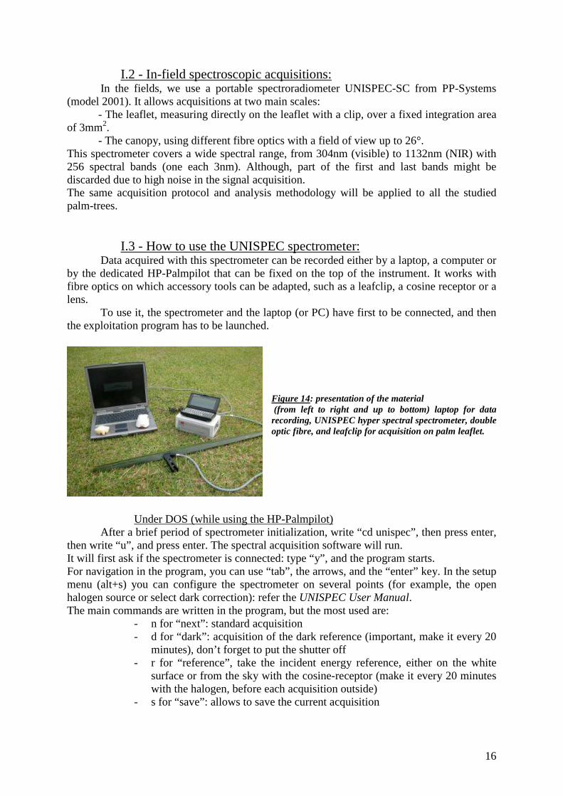
I.3 - How to use the UNISPEC spectrometer: Data acquired with this spectrometer can be recorded either by a laptop, a computer or by the dedicated HP-Palmpilot that can be fixed on the top of the instrument. It works with fibre optics on which accessory tools can be adapted, such as a leafclip, a cosine receptor or a lens. To use it, the spectrometer and the laptop (or PC) have first to be connected, and then the exploitation program has to be launched.

Figure 14: presentation of the material (from left to right and up to bottom) laptop for data recording, UNISPEC hyper spectral spectrometer, double optic fibre, and leafclip for acquisition on palm leaflet.

Under DOS (while using the HP-Palmpilot)

After a brief period of spectrometer initialization, write “cd unispec”, then press enter, then write “u”, and press enter. The spectral acquisition software will run. It will first ask if the spectrometer is connected: type “y”, and the program starts. For navigation in the program, you can use “tab”, the arrows, and the “enter” key. In the setup menu (alt+s) you can configure the spectrometer on several points (for example, the open halogen source or select dark correction): refer the UNISPEC User Manual. The main commands are written in the program, but the most used are:

- n for “next”: standard acquisition - d for “dark”: acquisition of the dark reference (important, make it every 20

minutes), don’t forget to put the shutter off - r for “reference”, take the incident energy reference, either on the white

surface or from the sky with the cosine-receptor (make it every 20 minutes with the halogen, before each acquisition outside)

- s for “save”: allows to save the current acquisition

17

Under Windows: Run the Uniwin_v3_0.exe program. If it is the first use of the program, the spectrometer calibration parameters have to be set in setup/system parameters:

- A= + 300.2246727 - B= + 3.339009727 - C= - 0.0003590946515

Then, the use of the program is the same than under DOS. Remember to always exit the program with data/exit and not with the cross on the upper right corner, otherwise the unit numbers aren’t saved...

II - The choice of vegetal material: II.1 - Choice of the palm-trees:

Our main goal is to classify the palm-trees by different degrees of sickness: healthy, low, medium or high degree of disease. For that purpose, we have to learn how to classify the palm-trees with infield observations, i.e. evaluate the apparent degree of sickness of a given tree. Then we take digital photos, note any observation that helps understand the palm status, and then do the spectral acquisition, beginning by the canopy-level measurements, followed by two leaves cutting down for leaf-scale measurements. A statistical model will be computed to discriminate the palm-trees according to their degree of sickness on the basis of two randomly selected thirds of this database. The last third will be used as a validation sample.

II.2 – Canopy measuring: The first acquisition to do is the reflectance spectrum of the whole canopy for the selected palm-trees. For that, we have to build scaffoldings around the palm-tree and to climb it to do our acquisitions. Then, we can do our acquisitions with the spectrometer on the canopy. For that, we use fibre optics having a field of view (FOV) of 26°. Considering that the palm-tree efficient diameter is less than 9 meters, and that the fibre optics placed at about 1m from the canopy integrates the spectrum of a target of less than 50cm in diameter, we need to sample several areas over the palm canopy. To get a good mean of the whole canopy reflectance, we propose to take one acquisition above the centre of the tree and then 3 to 5 more (depending of the possibilities) at about 1m from the centre, scattered over the canopy disk. This repetition of acquisitions should avoid the directional effects and decrease the small local heterogeneities.

Figure 15: picture of a canopy acquisition (The fibre optic is fixed on a boom, with a rocking system to keep the fibre optic vertical)

18

To be reliable, the acquisitions have to be done in a particular way: First, the offset and the reference acquisitions have to be done to correct the future

acquisitions. The offset is the dark acquisition and it is used to discard the acquisition’s background noise (it is done by hiding the optic fibre in the black foam and pressing the letter “d” on the laptop). The reference is the acquisition of the pure sunlight’s spectrum; it is used to calculate the reflectance (leaf reflectance = leaf radiance / incident light radiance). The reference acquisition is done by placing the cosine receptor at the end of the fibre optics looking towards the sky above the canopy, and pressing the letter “r” on the laptop. Then, after saving those two files, the acquisitions on the canopy can be done (typing “n” on the laptop).

Therefore, we acquire the offset, the solar radiance and then the canopy one. IMPORTANT : the dark-offset and reference acquisitions have to be done regularly for a good calibration of the spectrometer: The sunlight has variations over time, even in a perfect blue sky, and the spectrometer can have imperfections caused by heat or many things. The dark-offset can be acquired every 20 minutes, but the reference must be acquired before each canopy acquisition with the smallest time gap in between. The canopy-level acquisitions must be done before the cut of chosen leaves.

II.3 - Leaf and leaflets choice for optical acquisition on leaflets:

Figure 16: top sight of a palm-tree and selection of the leaves. The selected leaves in former studies are in green. Preliminary analyses showed that the discrimination works better on young leaves (5th and 9th), so we will finally cut only two young leaves. This allows us to do a less destructive study. WARNING : Cut the leaves only after the acquisition above the canopy!

The selected leaves are the 5th and the 9th because of several reasons:

- They are on both side of the palm tree, whatever could be the angle between leaves, - They belong to two different but adjacent spires on the palm, - They are on the upper side of the tree and are visible from the top of the palm-tree, so

they receive direct sunlight. For that, it will also be easier to compare our results with remote-sensing data during the study,

- They are young leaves and so aren’t covered by lichen (not as old leaves, since the 18th they are too much covered),

- Stress symptoms are visible on at least one of those leaves, Then, after the leaves cut, spectral acquisitions are done on several selected leaflets:

19

Figure 17: leaflets selection on the selected leaves. The selected leaflets are in green and named.

Some previous acquisitions revealed a great variability of reflectance from a leaflet to another. This could be caused by mineral gradients in the leaf. The insertion angle has also an impact on reflectance, because of the orientation of the leaflet in respect to the sunlight. So 5 leaflets where selected: the 10th, 35th, 55th, 70th and 85th, to cover the most variability over the leaf.

II.4 - Acquisitions on the leaflet:

Figure 18: Reflectance spectral acquisitions’ protocol on palm-trees’ leaflets

A previous study revealed variability in the reflectance along of the leaflet. So we have to concentrate our acquisition on small selected surfaces on the leaflets (around 2cm²), on both side of the central nerve. Because of the great variability along leaflets, we have to consider 2 zones for all the acquisitions: the first and the second third of the leaflet. Statistical tests revealed that 10 acquisitions on both side of the central nerve and on each third were necessary to be statistically representative of the leaflet.

20

40°

Fibre optique

Figure 19: The leafclip used for acquisitions on leaflets

The acquisitions have to be done in a particular way: we use a leafclip, and the spectra also have to be calibrated with a dark offset (same way than for the canopy, but you also have to close the shutter by pressing “del”), and a reference spectrum. This one is acquired on a standard plate, named “spectralon”, made of precipitated barium sulphate, which is an absolute white. Thus, the reference is a measured putting the clip on the edge of the plate and typing “r” on the laptop keyboard.

Figure 20: picture of the “spectralon”, in precipitated barium sulphate

WARNING : don’t touch the plate, because fingers leave traces on the surface, and calibration would be wrong.

As the offset has to be measured at least each 20 minutes, the reference has to be measured each time a new offset is acquired, so it has also to be done every 20 minutes.

II.5 - In-field Constraints: In Industrial palm-trees plantations, the trees are from 1.5 to 20 meters height. Their leaves are 5 to 8 meters long and composed by 250 to 350 leaflets of 1 to 1.5 meters long. Because of the height of trees and the number of leaves and leaflets, a local handling for leaflets acquisitions is dangerous and complicated. So we have to remove the selected leaves from the tree, and choose leaflets to do acquisitions at home. A former study revealed that the reflectance of the leaves isn’t modified until a few hours after being cut, so the acquisition on the leaflets has to be done as fast as possible after cut.

Optic Fibre

21

III – First results and expectations III.1 – Reminder of the main objectives

The main goal of the study is the classification of palm-trees in accordance with their ganoderma sickness degree, on the only basis of their reflectance spectrum. This spectrum could be acquired by spectroscopy, as described before or maybe by remote sensing (if conclusions of the final study declare it possible). Remote sensing could be a saving of time. For that, we will go in fields and locate different palm-trees in different degrees of sickness. We will visually estimate the disease degree according to several symptoms (cf. Pak Wahyu’s experience and training) and classify the trees into three or four classes (healthy, low, medium and high sickness). On the selected palm-trees, we will do the reflectance spectroscopy acquisitions described in part II, and make them correspond to our visual diagnostic in the database. With statistical analysis, we will see if we can discriminate between the different classes only with spectral data (the visual diagnostic contributes to verify if the discrimination is good).

III.2 – First results In previous acquisition campaign (focusing on nutrition stress), only nine palm-trees canopy’s spectra where acquired: 3 palm-trees were in good health, 3 were on medium sickness and 3 were highly infected. A simple statistical processing then allowed a good discrimination between the three classes: first applying a polynomial smoothing and a derivation of the spectra (Savitsky-Golay filter), followed by PCA (Principal Component Analysis), and FDA (Factorial Discrimination Analysis) applied to PCA scores lead to the split of the three populations in different areas of the FDA space (cf. Brégand, 2007).

Figure 21: Representation of the different individuals in the two first principal layouts of the FDA (applied to the PCA’s scores, applied the second derivation of the spectrums of the canopy)

Legend: N No infection M Medium infection H High infection

22

We can see a great discrimination of our nine palm-trees: the healthy (N) and the sick (M and H) palm-trees are separated by the line of equation x=0. The medium (M) and the high (H) infected trees are then separated by the straight line of equation y=0. We thus have a perfect discrimination between infected palm-trees and healthy ones, and between the different degrees of disease (in a total of 3 classes). Now it has to be validated with a larger data set, and to be tested at each scale: canopy, leaflet, and remote sensing.

III.3 – Deepening of the study The previous study underlined a possible way to discriminate the palm-trees between their ganoderma infection degrees, but only on a very small sample, which is not statistically correct. Therefore, it is now necessary to repeat the operation with more palm-trees for a statistically strong model: the present study consists in acquiring a bigger database (at least 100 individuals; the more the better) and in doing the same statistical processes. If it does not work anymore, we will text other statistical methods of discrimination. We will first try with four classes (the better), then three, or two (sick or not) if it does not work with more. If the model appears to be statistically strong, we will validate it. Then we will analyze if we can have the same results with remote sensing, deciphering which spectral bands are the most useful to discriminate the infection because the UNISPEC spectrometer has 256 bands, while airborne sensors might reach this capabilities at high costs but satellites sensors have only very few bands (most have only 4). With this tool, we will be able to follow the development of the ganoderma, act cleverly understanding it, and maybe control it, or find a solution...

IV - The different nutritive stresses and ganoderma disease: IV.1 – Stress, ganoderma and potential need of foliar analysis:

In field, many Palm-trees can suffer nutritive stresses caused by a lack of nutrients or/and trace elements: nitrogen (N), potassium (K), phosphorus (P), magnesium (Mg) and Iron (Fe). For a better action and for soils preservation, it is important to identify the missing element for an effective fertilization. If reflectance spectrometry makes it possible for Nitrogen and Phosphorus, it is not very accurate and it cannot detect stresses caused by the missing of the other nutriments. So the better way still is a foliar diagnostic: the different lacks cause particular effects on the leaves, and were analyzed and classified by Fairhust and Caliman, 2001. As we saw earlier, the ganoderma blocks the vascular tissues of the palm-tree and so he cannot raise the sap, which brings water and nutriments. So the ganoderma causes different stresses on the trees as water stress or nutriment stress, and it is sometimes hard to differentiate a sick palm-tree and an only stressed palm-tree (not infected with ganoderma). So we could need some analysis to differentiate those trees, especially for the low infected ones. Those analysis would be to see if there is mycelium or not (if the palm is infected by ganoderma or not).

We could also need foliar analysis to complete the database of the previous study about prediction of the nutriments’ concentration in the leaves by spectroscopy. For that we will try to find 10 to 15 specific cases showing specific lack in one nutriment. With those typical cases, we could improve our leaves’ concentration of nutriments’ prediction model

The foliar analysis is always done on leaflets implanted near the B point, which is the point where the rachis’ section change and become circular, and it a reference point in palm-trees studies.

23

IV.2 - Nutritive stresses: Analyze and classification by Fairhust and Caliman of the visible symptoms of

nutritive stresses is presented in the following board: Missing element Symptoms Picture

Nitrogen (N)

The photosynthesis pigments are affected; the leaflets become pale green and progressively yellow with the stress’ intensification. The youngest leaves are the first affected. The palm-tree and leaves grown slower and production is affected. Figure 22: to upper leaves of a palm-tree suffering

a lack of Nitrogen

Phosphorus (P) There isn’t a visible symptom on the leaves, but the palm-tree and his leaves grow slower.

Potassium (K)

Orange-spotting: discoloration of the older leaflets in pale green spots, then yellow and orange with the accentuation of the lack. This lack can be responsible of a 20% production loss.

Figure 23: Orange spotting on a palm-leaf

Magnesium (Mg)

Discoloration of the older leaves in yellow, then orange, then red. When the lack increase, the discoloration rise to the top of the tree (to the younger leaves). The most discolorated leaves are the most exposed to the sunlight. Figure 24: High Mg stress, the leaf is discoloured

in pale green, yellow and red.

Iron (Fe)

Discoloration of the 3 to 4 youngest leaves (on the top of the tree). They become pale green then yellowish green.

Figure 25: comparison between a normal palm-leaf (on the left) and a young palm-leaf suffering

Iron lack (on the right)

24

Part C – In-field application

I – Acquisitions I.1 – A weather dependent acquisition campaign

An important point in this acquisition campaign is the weather dependence of outside radiometric acquisitions. Even if it is not the case with spectrophotometry because the reference incoming light and the object radiance are acquired in the same time, the spectroradiometry, where reference and object acquisitions are done separately, need a very stable weather. Actually, a brief period between the reference acquisition with the cosine receptor and the canopy’s radiance acquisition still exist, due to the change of device (removing the cosine receptor or changing the fibre optics) and the limited speed of the Palmpilot. Therefore, if the incident light changes during this period, the acquisition will be false and unusable. This acquisition campaign needs a sunny stable weather for good canopy acquisitions. The clouds will interact in the measurements absorbing in Near InfraRed with different degrees depending on their thickness, in an unstable way, and will false the acquisitions. This is a big constraints in tropical climate, where the measurements can mostly be done between two clouds in brief stable sunlight conditions. In the fields, to get enough and stable light to be reliable, measurements were limited to the timetable 8:30am and 4:00pm. Even if the sun rises at 6:00am and the sun lies at 6:00pm, we cannot do acquisitions while light is quickly changing (during sunrise and sunset). As an example of the variations of the incoming light according to the daytime, we can present a graph of acquisitions made in Montpellier, France, but which illustrates well those variations (figure 26):

Figure 26: Evolution of the diffuse incoming sunlight according to the moment of the day

25

A particular attention is thus set on the weather: if it is unstable, too cloudy or rainy, the canopy acquisitions aren’t made, and we find something else to do (e.g. statistical data analysis, or leaflet acquisitions on old palms that are too tall to be measured in the fields).

I.2 – Canopy acquisitions The canopy acquisitions are made by placing the fibre optic responsible of the measurement at least at 1 meter above the canopy. So this can be difficult for the older palm-trees reaching 15 to 20 meters! For that, the acquisitions are just made on young ones at 5 to 7 meters height. We use scaffoldings to climb at the canopy level. We fix the fibre optics on a wooden stick to reach one more meter and a half (see figures 27 and 28).

Figure 27 (left): the scaffolding used for canopy acquisitions

Figure 28 (right): the stick

with a system attaching fibre optics above the

canopy

Six acquisitions are made for each palm-tree, by placing the scaffolding on two opposite sides of the tree and making three acquisitions per location, moving on the platform. With those six acquisitions angles, we reduce the variations due to the position of the measurement.

Figure 29: The different angles of the six acquisitions on the canopy The palm-tree is given an identification number in accordance with its position in the palm grove. The ganoderma sickness degree is confirmed and recorded, as well as a diagnostic of possible nutriment deficiencies. Pictures of the whole tree (stem to canopy) are also taken. Thanks to all these observations, we will be able to manage a whole database and to understand possible discrimination errors in the later statistical processing.

Scaffolding positions

Acquisition directions

26

Then, when the measurement is complete, we cut the leaves number 9 and 5, on which we select the leaflets described in the protocol to bring them home for indoor acquisitions at the leaflet level.

I.3 – Quickbird acquisition A Quickbird image of a large part of the palm grove was acquired in June 2008 (Cf. Appendix 3 & 4). This image is useful for two reasons: first, it is a good way to follow our acquisitions in the fields (with 7,250ha, it can be hard without a map!), to control and choose the palm-trees; and it will be useful to extend our data to remote sensing.

After each acquisition, each measured palm-tree location and its disease index are picked in a vector layer on this image. Thus, we can see the covered areas, and extract radiometric data out of the image for each palm-tree. Knowing their sickness degree, we will be able to test if the same discrimination than for field canopy or leaflet data is still possible with only four spectral bands.

An important point is that the image data are in radiance. We will thus have to convert these data into reflectance. For that purpose, we measured the reflectance of several invariant surfaces all around the area (roads, buildings, bare soil ...) that are easy to locate accurately in the image. Then we search a linear regression between field-measured reflectance and image radiance to extrapolate the reflectance calculation at the whole image scale. Even if the discrimination will probably not work with only 4 spectral bands, it is an important step of the study to prepare the future: in some years (in five to ten years, at most) several hyperspectral satellite providing a hundred of bands will be available.

II – In-situ adaptations II.1 – An ergonomic way to do canopy acquisitions

Doing stable acquisitions over the canopy of a tree is difficult: the measurements have to be comparable for one tree to another, and with a scaffolding and a stick, we create a great variability in the fibre optics position. To avoid this problem, Dr. Camille Lelong created a clever device to fix the fibre optics angle for each acquisition.

This invention does not have a patent yet, but it should… fixed at the top of the stick, it maintain at the same time a vertical fibre optics for reference acquisition with a cosine receptor, and a second fiber optics with an angle of 40° for the canopy radiance measurements. A patellar rolling system with weights allows the device axe to be always vertical, whatever could be the stick angle! With this system, we can easily acquire stable and comparable data.

Figure 30: The genius 40-constant-acquisition-degree invention

Fibre optics #2 with cosine receptor

Fiber optics #1 making a 40° angle with the principal axe

Rocking system maintaining the principal axe vertical

Principal axe

Weights

27

II.2 – Managing two fibre optics A problem with the UNISPEC-SC spectroradiometer is the presence of only one

acquisition channel. For that, the reference acquisition and the canopy acquisition have to be done separately. While using a 1.80m stick above the canopy, putting on and out the cosine receptor at the end of a single fibre optics was not compatible with the absolute necessity to make the two acquisitions in a very short time. Thus, we decided to use two fibre-optics: they are both fixed at the stick, one with the cosine receptor for the reference, one in the direction of the canopy. Therefore, we just have to change the input fibre optic on the spectroradiometer, which takes around 3 seconds, instead of taking back the stick, removing the cosine receptor, etc...

1) Due to differences in fibre optic conception (e.g. field of view, absorption ability…), two different fibre optics do not measure the same amount of radiance for the same target in identical conditions.

2) Due to the scattering material that is somewhat semi-transparent, the cosine receptor (CR) transmits to the fibre optic a smaller amount of radiation than it receives, so the measured intensity is decreased compared to acquisition with the fibre optic alone.

For these two reasons, the device presented here, composed of two different fibre optics and one cosine receptor has to be intercalibrated to allow the derivation of the reflectance.

- Actually, the reflectance of the target, Rt, is the ratio

of the target radiance measured by the FO-I = It, by the radiance of the incident light measured by FO-I without cosine receptor = I01.

- Practically, the incident light is measured with FO-II: I02.

Rt = It/ I01 = (It/ I02) * (I 02/ I01) = K2/1 * I t/ I02, where K2/1 is the coefficient of calibration of FO-II+CR and FO-I.

To derive K2/1, we acquired a set of measurements with the spectrometer, on a white target for instance. For each wavelength, we calculate the ratio of the radiance measured with FO-II and the cosine receptor on the radiance measured with FO-I on this same target. It is better to do several calibration measurements to ensure the stability of this coefficient and get a robust mean.

All our reflectance calculations from our canopy acquisitions where multiplied by this K2/1 coefficient to correct the data.

28

II.3 – The edification of IDL routines In view of the numerous acquisition files created by the measurements on canopy and

leaflets (6 canopy and 40*6=240 leaflet acquisitions for each tree) a manual treatment of the data seemed impossible. For that, I developed several data processing programs under IDL, adapted for the needs of the study. There are three kinds of programs:

- A program for the treatment of the canopy acquisitions, recapping the wavelength, the 6 acquisitions and their mean in a single text file for each tree, and a text file recapping the palm-tree names, wavelength and all canopy means in rows or in columns, for the following statistical treatments

- A program for the treatment of the B leaflets, with the same properties as the routine for the canopy

- A program for the treatment of all the other leaflets acquisitions, recapping for each leaflet the wavelength, the 40 acquisitions and their mean, and for each leaf the wavelength, the different leaflet means and the means at leaf scale. In each tree folder it creates a text file for each leaflet of each leaf, and a text file for the leaf mean. It also recap all the both leaf means of each tree in a single text file, in rows or columns, for later analyzes.

Those programs are available with two options: processing the data of a single tree,

creating a graph to check if there are problems in the acquisitions, or processing the whole palm-trees, without data check, to create the global text file. The first option is set first, just after the acquisitions, and the good data are sorted and used for the global text file.

The development of those programs involve the necessity of a strict sorting of the acquired data in particular directory for all trees, so that the routines can easily find the different data in a uniform arborescence.

III – First point after a week of acquisitions III.1 – Number of acquired data

It is important to underline the fact that this week was the first one of the acquisition campaign, and so the methods had to be set for the first time. For instance, we encountered a few problems with the spectrometer itself. Therefore, the next acquisitions will be done a little faster (the campaign is now launched!).

We made 7 days of real acquisitions and spent 3 days in visiting the palm grove, going in town to repair the spectrometer and making acquisitions for the quickbird image calibration. So, in 7 days, we acquired the canopy reflectance of 13 palm-trees and the leaflet-scale reflectance of 20 palm-trees. This difference is due to bad weather conditions (cloudy sky, even rain) during the week, which didn’t allow us to do many canopy acquisitions. During those cloudy days, we only cut two leaves for leaflets reflectance acquisitions on old palms, too high to be reached with scaffoldings without danger.

In those 20 leaflet acquisitions, we have 5 healthy and 15 sick palms: 2 of low degree, 8 of medium degree, and 5 of high degree of infection. In the 13 canopy acquisitions, we have 4 healthy and 9 sick palms: 1 of low degree, 6 of medium degree, and 1 of high degree of infection. Of course, we have to take care of our measurements during the whole campaign to have a balanced proportion of sickness degree at the end of the study.

III.2 – Acquisition speed and predictions

With this week of work, and the improved organisation of the campaign, we can evaluate the time of the different acquisitions.

29

In a sunny day, we can make canopy acquisitions on three palms during the morning, and then make the leaflet acquisitions on the same three trees during the afternoon. In a cloudy day, we can cut leaves on 4 to 5 palm-trees and make the leaflet acquisitions at home. Of course, this can be adapted compared with the occurrence of cloudy days: if there are not many sunny days, we will use them to do the more canopy acquisitions than possible, and cut the leaves on cloudy days. So we also can do 5 canopy acquisitions on sunny day, and also one to two leaflet acquisitions after that (the 4 other trees will be processed on a rainy day).

Between 10 august (today) and the 22 October (few days before leaving) there is 73 days. In those we can subtract 10 Sundays, maybe 8 days without work (due to problems or to local holidays, like the 18th of August, or the 1st and 2nd of October) and 3 days of in-field observations to spot some new sick palm-trees for remote sensing processing (those trees aren’t acquired). Therefore, we keep 62 days of real work.

We can consider 3 kinds of weather conditions during the campaign:

- Good conditions: 42 sunny days and 20 cloudy ones - Medium conditions: 32 sunny days and 30 cloudy ones - Bad conditions: 22 sunny days and 40 cloudy ones

On each of those conditions, we can both do normal canopy acquisition (3/day) or intensive (5/day). Those numbers are just indicative. At the end of the campaign, we will then have:

- In Good conditions: between 42*3+13 = 137 and 42*5+13 = 223 canopy acquisitions, and between 42*3+20*4+29 = 226 and 42+20*4+20 = 142 leaflet acquisitions, according to the chosen intensity of canopy acquisitions during sunny days.

- In Medium conditions, between 32*3+13 = 109 and 32*5+13 = 173 canopy acquisitions, and between 32*3+30*4+20 = 236 and 32+30*4+20 = 172 canopy acquisitions.

- In Bad conditions, between 22*3+13 = 79 and 22*5+13 = 123 canopy acquisitions, and between 22*3+40*4+20 = 246 and 22+40*4+20 = 202 canopy acquisitions.

It is normal that the number of leaflet and canopy acquisitions is unbalanced: this is

due to the inaccessible character of the older palm-trees for the canopy acquisitions. We can evaluate to around 35% the difference between the 2 numbers.

We see that we can reach our goals of 100 acquisitions in terms in several cases, adapting in accordance to the weather to have the number of acquisitions we want on both kind.

30

Part D – statistical analysis

I – Acquired Data and Pre-treatment I.1 – Total Acquired data

At the end of the acquisition study, we have 102 canopy acquisitions and 117 leaflet ones. Those acquisitions are distributed as following:

Canopy Leaflet Skor 0 40 32 Skor 1 21 33 Skor 2 37 33 Skor 3 4 19

TOTAL 102 117 We see that we reached our goal of 100 acquisitions of both canopy and leaflets. We also almost reached our predicted number, but we had to face several problems of staff availability some days, had an entire week of rain, etc... An important point is the lack of Skor 3 in canopy acquisitions. It is caused by the low number of trees highly infected by ganoderma, and by the fact that they are almost dead at skor 3, and were often fallen down when we came for doing the acquisitions.

I.2 – Sorting the data I.2.1 The necessity of sorting the data:

In any acquisition campaign, there are bad acquisitions. There can be many reasons that we don’t always know. For this campaign, it can be caused by early or late acquisitions on canopy, when the sun is low and the light changing fast, it can also be caused by unstable weather, or wet leaves, etc... Therefore, we have in the data some very strange spectra (eg. reflectance above 1 or negative) that have to be deleted. This has to be done before the statistical analysis. There are also wavelengths with a lot of background noise and which are problematic for the statistical analysis, especially in the UV domain and in the longer wavelengths in the NIR. These wavelengths have to be discarded. So we just keep the wavelengths between 450nm and 1100nm for the statistical process.

I.2.2 Creation of the database After the deletion of the abnormal spectra in canopy acquisitions, the final database used in this study is composed as following:

Skor 0 Skor 1 Skor 2 Skor 3 Total Number 36 20 36 3 95

31

The different statistical treatments will be made on this final database for two kind of discrimination: 2, and 4 degrees of sickness.

I.3 – Pre-treatment of the data for the PLS-DA application

In addition to the necessity of sorting the data to delete the abnormal spectra, we will do some pre-treatments to improve the statistical analysis. Those pre-treatments are:

� the use of the logarithms of spectra, because the PLS and PCA methods are based on linear combination, and the logarithms will avoid the bad translation of multipliers

� a calculation of real PLS coefficients for each class with an unmixing (in the ENVI environment). The different classes are coded by numbers, from 0 to 1, as if it was concentrations. Skor0 are 0 and skor3 are 1. This method allowed, by a linear combination, to solve the problem: skor1= ? x skor 3

� a smoothing and derivative treatment on the data by the Savitsky and Golay method (1964). This treatment allows calculating derivative spectra for several derivative orders and using a polynomial convolution function smoothing the different spectra.

This Savitsky-Golay method in reflectance analysis allows eliminating background signals. The calculation of derivative spectra reduces the low frequency background noises and the overlapping spectra (as soil effect for example) (Butler and Hopkins, 1970). This effect increases with the derivative order. The high frequency background noises are increased with the derivative order, but the polynomial convolution allows avoiding this effect. The use of derivative spectra allows underlining important part of the spectrum, as red-edge for example, which is important for estimating chlorosis. But as we saw the canopy architecture effect is reduced with derivative order, and in our study, it has an importance: the canopy structure is modified with ganoderma infection. So we won’t use too high derivative spectra: degree 0, 1 or 2 at maximum.

32

Figure 31: Comparison of Untreated and First derivative spectra for the same palm-trees; we can see that the red-edge (700nm) is underlined, as the green pick.

For a complete and powerfull statistical analysis, we will use a large panel of

combination of the different Savitsky-Golay parameters: 1. width of the smoothing window (5, 9, 11, 13, 17, 21, 31, 41 and 51) 2. order of the modelising polynomial (2 or 3) 3. derivative order (0, 1 or 2)

33

II – Presentation of the PLS-DA method II.1 – The PLS theory: (Tenenhaus, 1998)

The PLS (Partial Least Squares) can be used when there is only one variable Y to explain (PLS1) or several variables Y (PLS2). Here we will only treat the PLS1, the PLS2 theory can easily be extended from the PLS1 one. The PLS regression is perfectly adapted to our data set. It can be applied in the case where there is a lot more explicative variables X than observations. Moreover, those X variables can be strongly correlated (this is the case with the many spectral bands). We can summarise the PLS regression as a succession of simple linear regressions: we

first build a component1 11 1 1... p pt w x w x= + + , where 1

2

1

cov( , )

cov ( , )

jj p

jj

x yw

x y=

=

∑.

Then we do a simple linear regression of y on 1t : 1 1 1y c t y= + , where 1c is the regression

coefficient and 1y the remainder vector. So we have a first regression equation:

1 11 1 1 1 1... p py c w x c w x y= + + +

Then we can, if the explicative power of this equation is insufficient, build a second component2t , linear combination of the remainders 1 jx of the regressions of the variables jx

on the component1t . We obtain 2t by this formula: 2 21 11 2 1... p pt w x w x= + + , where

1 12

21 1

1

cov( , )

cov ( , )

jj p

jj

x yw

x y=

=

∑. We do a regression ofy on 1t et 2t : 1 1 2 2 2y c t c t y= + + .

This iterative process can be followed using at the same way the remainders 2 21 2, ,..., py x x of

the regressions 1, ,..., py x x on 1 2,t t . The number N of components 1,... Nt t to conserve is

generally set by the cross-validation. We then calculate two criteria for helping the decision: the hRSS(Residual Sum of Squares) and the hPRESS (Prediction Error Sum of Squares) :

$( )$( )

2

2

( )

h i hi

h i h i

RSS y y

PRESS y y−

= − = −

∑

∑

34

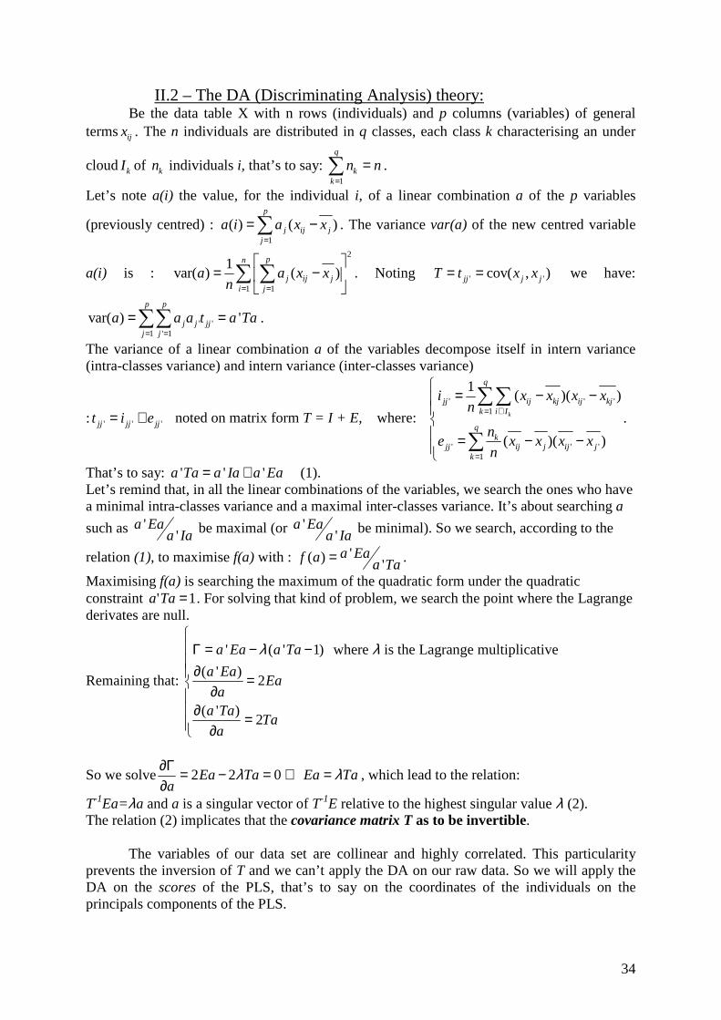
II.2 – The DA (Discriminating Analysis) theory: Be the data table X with n rows (individuals) and p columns (variables) of general terms ijx . The n individuals are distributed in q classes, each class k characterising an under

cloud kI of kn individuals i, that’s to say: 1

q

kk

n n=

=∑ .

Let’s note a(i) the value, for the individual i, of a linear combination a of the p variables

(previously centred) : 1

( ) ( )p

j ij jj

a i a x x=

= −∑ . The variance var(a) of the new centred variable

a(i) is :

2

1 1

1var( ) ( )

pn

j ij ji j

a a x xn = =

= −

∑ ∑ . Noting ' 'cov( , )jj j jT t x x= = we have:

' '1 ' 1

var( ) 'p p

j j jjj j

a a a t a Ta= =

= =∑∑ .

The variance of a linear combination a of the variables decompose itself in intern variance (intra-classes variance) and intern variance (inter-classes variance)

: ' ' ' notée sous forme matricielle jj jj jjt i e T I E= + = + , ' ' '

1

' ' '1

1( )( )

où :

( )( )

k

q

jj ij kj ij kjk i I

qk

jj ij j ij jk

i x x x xn

ne x x x x

n

= ⊂

=

= − −

= − −

∑∑

∑.

That’s to say: ' ' 'a Ta a Ia a Ea= + (1). Let’s remind that, in all the linear combinations of the variables, we search the ones who have a minimal intra-classes variance and a maximal inter-classes variance. It’s about searching a

such as ''

a Eaa Ia be maximal (or '

'a Ea

a Ia be minimal). So we search, according to the

relation (1), to maximise f(a) with : '( ) 'a Eaf a a Ta= .

Maximising f(a) is searching the maximum of the quadratic form under the quadratic constraint 1' =Taa . For solving that kind of problem, we search the point where the Lagrange derivates are null.

Remaining that:

' ( ' 1) où est le multiplicateur de Lagrange

( ' )2

( ' )2

a Ea a Ta

a EaEa

aa Ta

Taa

λ λΓ = − −∂ = ∂

∂ = ∂

So we solve 2 2 0Ea Ta Ea Taa

λ λ∂Γ = − = ⇔ =∂

, which lead to the relation:

T-1Ea=λa and a is a singular vector of T-1E relative to the highest singular value λ (2). The relation (2) implicates that the covariance matrix T as to be invertible. The variables of our data set are collinear and highly correlated. This particularity prevents the inversion of T and we can’t apply the DA on our raw data. So we will apply the DA on the scores of the PLS, that’s to say on the coordinates of the individuals on the principals components of the PLS.

noted on matrix form T = I + E, where:

where λ is the Lagrange multiplicative

35

II.3 – Principle, objectives and use of the PLS-DA The PLS can be applied by two points of view: 1 - The first kind of application concerns the prediction of variables of “content” type. Using a learning set, the PLS creates a model of relation between X and Y. Then, we apply this model which predicts the variable Y on a test set where the Y variable isn’t specified. 2 - We also can use the PLS as a regression for “compression” of the information, on a high number of reasonable components for then applying a DA on the obtained scores.

With the results of the unmixing method, we found that, approximately,

Skor1 = 0.6 * skor0 + 0.4 * skor3 + 0.005 Skor2 = 0.4 * skor0 + 0.6 * skor3 + 0.007 So, with those results, the PLS coefficients given to the explicative variable Y of each class were:

� 0 for the healthy palm, � 1 for high sickness degree, � 0.4 for a low one, � 0.6 for a medium one.

The use of those coefficients instead of discrete ones (a different number for each class) was made because the PLS method is used to calculate continuous variables and not discrete ones; if we use for example 0, 1, 2, 3 for each class, the RMSEP is high… Moreover, this is quite coherent with a sickness degree which is a continuous phenomenon, and not a discrete one. This method will be applied on the pre-treated spectra of the canopy and leaflet acquisitions for the gain of quality and information on the pre-treated data. To use the PLS-DA method, we had the R program. We use the PLS to compress the information from 256 components (256 bands) to less than 10 ones, and then we apply the Discriminant Analysis on the loadings of the PLS (i.e. the coordinates of each palm-trees in the new space defined by the new compressed variables). The PLS is cross validated with a leave-one-out method, and it is the same for the DA. So we use the full dataset to build and validate the model.

36

III – PLS-DA Treatment III.1 – PLS-DA on the spectra acquired on canopy

III.1.a – First observations about the statistical treatments:

After the first tests of statistical analysis, we went to few observations, leading to the best results:

� The PLS-DA method is always better than the PCA-DA one for that kind of classification

� The discrimination of sickness degree is better with the logarithms of the spectra (the PLS method is a linear combination of the different components of the spectrum, and the logarithm form allows to “transform” the multiplication in addition, and so to simplify the PLS)

� The statistical treatment shows better results width small width for the smoothing window of the Savitzky-Golay method

� The results are also better with derivative spectra (degree 1 or 2) � The classification is often better with a model built with a polynomial of third

degree.

Those results were obtained by many observations and different tests for the sickness degree discrimination. Those different tests were made on different databases, with different SG combinations. All those tests are presented in Annex 5.

The following results just show the best results for each kind of discrimination.

III.1.b – 4 classes discrimination The best results are seen with the SG combination w9o3d2 and w11o3d1 (width -

polynomial order – derivative degree).

W9o3d2 We took 7 PLS components, resulting in a R²=0.79561 and a RMSEP=0.1310.

Those results are pretty good; the R² is high and the RMSEP is low enough for the different classes to not cross themselves (Skor 0 = 0, Skor 1 = 0.4, Skor 2 = 0.6, Skor 3 = 1)

Figure 32: Presentation of the graph of evolution of R² and RMSEP according to the number of PLS components

37

So the model is well built, and the Discriminant Analysis on the loadings of the PLS model shows a good discrimination of the different classes:

Skor0 Skor1 Skor2 Skor3 Good discrimination

Skor0 34 2 0 0 94,44% Skor1 0 17 3 0 85,00% Skor2 0 2 34 0 94,44% Skor3 0 0 0 3 100,00%

Total good discrimination 92,63%

Figure 33: representation of the palm-trees in the new AFD coordinate system (built with the PLS scores) –

skor0 are in black, skor1 in green, skor2 in yellow and skor3 in red.

So we can see a good PLS model and a good discrimination between the different

sickness degrees, even in the lowly infected palm-trees (even if in early stages, the discrimination is less powerful). Even in the graph 33 we can see a good split of the different sickness degrees.

An important point with this classification is that none sick trees are considered as healthy, and in the same way, there are very few false alarms (around 5%), so not many healthy trees will be considered as sick.

We see that the discrimination between healthy and sick trees is quite powerful, but it

would be interesting to see if it is better when we build the PLS model considering only 2 classes: healthy palm-trees (Skor 0) and sick ones (Skor 1, 2 and 3)

38

III.1.c – 2 classes discrimination

For that kind of discrimination, considering just healthy and sick palm-trees, we could see the better results with the w11o2d1 SG combination. The model is built with 10 PLS components, resulting in a R²=0.6758 and a RMSEP=0.2779. We can see that the R² is lower than previously, and the RMSEP is higher, but it is because of the high variability of spectra values in the sick class (it regroups skor 1, 2 and 3). The higher RMSEP is also caused by a bigger value difference between the 2 classes which takes the values 0 (for healthy) and 1 (for the sick ones).

Figure 34: Presentation of the graph of evolution of R² and RMSEP according to the number of PLS

components So we have a quite a model less strong than previously, but still good enough for what

we want. The results of the discriminant analysis on the PLS loadings are very good:

Healthy Sick Good discrimination

Healthy 36 0 100,00% Sick 0 56 100,00%

Total Good Discrimination 100,00%

So we can see a perfect discrimination of the 2 classes: the model is strong, and

doesn’t make a classification mistake between sick and healthy palm-trees. The only problem is that we don’t have information about the sickness degree (and so the emergency of intervention) if the model is used later…

40

III.2 – PLS-DA on the spectra acquired on leaflets The PLS-DA on leaflet spectra doesn’t work, for leaflet means as for B leaflets. The statistical analysis can’t manage to build a PLS model, the R² is negative and the RMSEP is highly superior to 1, which is impossible. So the statistical analysis can’t find links between the disease infection degree and the spectra at the leaflet scale. A visualisation of those spectra underlines the fact that they are all very close, even between different classes. There is not especially any global aspect for each class, and spectra are very similar from one class to another. So it seems that the PLS isn’t able to find relationship between skors and spectra due to their similarities between classes. Calculating the mean difference between the different classes, we see that it is 5 times littler with leaflet spectra (0,0024) than with canopy spectra (0,0123).

Figure 35: Comparison of the mean spectra of each class from canopy acquisitions and leaflet acquisitions

41

Conclusion and perspectives This study consists in the verification and validation of a possible way to discriminate, by remote-sensing, observed palm-trees between four ganoderma infection degrees: no, low, average and high infection (respectively scores 0, 1, 2 and 3). The proposed methodology revealed relevant in previous studies, but only tested on a small sample of nine palm-trees. New field acquisitions were thus achieved during three months (august-october 2008) to improve the reliability of the model with a larger sample of palm-trees (around 100) at both the canopy and the leaflet scales. This document first presents the background of oil palm diseases issues and theory of reflectance spectroscopy on vegetation. Then it describes the experimental protocols and the field campaign to acquire the data. Then it focuses on the statistical analysis achieved in the aim of discriminating tree sanitary status. Only the canopy acquisitions were processed, due to first observations of “sunk” information in the leaflet-scale measurements. Data were then analysed through statistical routines, combining Partial Least-Square Regressions and Factorial Discriminant Analyses on one hand (PLS-DA), and Principal Component Analyses and Factorial Discriminant Analyses on the other hand (PCA-DA). Analyses were achieved on a large panel of databases derived from the canopy reflectance spectra, resulting from Savitsky-Golay filtering with varying parameters of smoothing-window width, polynomial degree, and derivation degree applied on both original and logarithm spectra. Among the huge number of tests, we only retained the most relevant to be presented here. The results show a good discrimination of the palm-tree sickness degree, which is even perfect when considering only two classes (sick vs. healthy trees). When considering four classes, which is even more relevant in the plantation management, global precision of the classification reaches 93%, still a very good score. Indeed, we point out the absence of misclassification of sick trees in healthy ones, which means that as long as a palm-tree is affected by ganoderma, it will be detected: this is quite important. On the other hand, the analysis leads to a low number of false alarms (around 5%): very few healthy palm-trees would be classed as sick We also show that is it very difficult to discriminate the low ganoderma infection on palm-trees (skor1). It may be caused by the way the infection degree is diagnosed in the field, which has very subjective and hazy limits, and considers both stem and canopy conditions. As an example, a palm-tree can be considered having a “score 1” if it has a perfect canopy but fruiting bodies at the bottom of the stem, or with no fruiting bodies and a very affected canopy… while we only have information on the canopy and not on the stem by remote sensing. Misclassifications can thus be explained by this technical limit in one part and field diagnostic fuzziness in the other part.

Although, this methodology seems inappropriate to process leaflet spectral acquisitions. This can be explained if the leaf composition and structure are just slightly modified by ganoderma before high infection, and for sure by the localized character of these alterations. Leaflet reflectance acquisitions are made on a tiny spot that might miss any specific leaf alteration area, even with a good sampling protocol. On the other side, leaf

42

thinning, yellowing or necrosis appear only randomly among the total amount of leaves. Therefore, the leaf sampling, even if selecting in theory characteristic ones, leads of course to the possibility of missing the symptoms. On the contrary, canopy reflectance reveals modifications in the tree structure, density (LAI) and architecture, as long as an integration of all the local perturbations in the leaves. It is thus more powerful to detect a global modification due to the disease. Finally, we can say we have a strong model and reliable results for the effective estimation of ganoderma infection of oil-palm trees based on canopy reflectance spectrum acquisitions. Those results might be applied to satellite remote sensing images, to cover a whole palm grove quicker and more easily. In theory, this should work, as the measurement is quite comparable and gives the same surface parameter: the canopy reflectance. But a first limit is that automatic extraction of the palm-tree radiometry is not yet reliable: it still has to be extracted “by hand”, leading to a very long process. But, more critical, only a poor spectral signature, featuring only four large bands (blue, green, red and near-infrared), is available at the moment from satellite multispectral imagery. At this spectral richness level, the discrimination is not effective at all. So this remote-sensing method could only work with airborne hyperspectral devices (such as CASI or HYMAP, for instance) or maybe with future satellite projects that should be launched after 2010 (eg. EnMap- GFZ Potsdam, Hypseo- ASI), but this still have to be validated with actual data.

43

Bibliography Andrieu B., F. Baret, S. Jacquemoud, T. Malthus, M.D. Steven (1997), Evaluation of an improved version of the SAIL model to simulate bidirectional reflectance of sugar beet canopies, Remote Sensing of Environment, 60(3):247-267 Baret, F. 1999. Potentiel de la télédétection pour l'agriculture de précision. L'enjeux français de l'agriculture de précision , pp. 8-11 Bjørn-Helge M., Ron W., 2007 : The pls Package : Principal Component and Partial Least Squares Regression in R. Journal of Statistical Software, Volume 18, Issue 2. Bonn F. et Rochon G., 1992 : "Le rayonnement électromagnétique : un support d'information", in Précis de Télédétection, Vol.1 : Principes et méthodes, Editions Universités Francophones, Presses de l'Université de Québec, p23-56. Brach, E.J., A.R. Mack, and G.T. St-Amour. 1981. Mobile field laboratory instrumentation to measure spectral characteristics of agricultural crops 626. Engineering and statistical research institute Bregand S., 2007 : « Analyse des comportements statistiques de la réponse spectrale des palmiers à huile aux stress nutritionnels et sanitaires », Mémoire de stage de Première Année de Master Professionnel en Mathématiques Appliquées, UFR Sciences et Techniques de Besançon, 72 pages. Fairhust,T., Caliman, J.P., 2001. Symptômes de déficiences minérales et Anomalies chez le Palmier à Huile (Elaeis guineensis Jacq.). Paris : Institut des phosphates et de la potasse (PPI) et CIRAD, 2001, 59 pages. Fairhurst T., and R. Härdter (eds). 2003. Oil Palm Management for Large and Sustainable Yields. PPI/PPIC and IPI, Singapore. 384p. ISBN 981-04-8485-2. 176 mm x 253 mm. (Second print) Gorry P.-A., 1990 : General least-squares smoothing and differentiation by the convolution (Savitzky-Golay) method. Anal. Chem., 62, p570–573. Guyot, G. (1989). Signatures spectrales des surfaces naturelles. Caen, Paradigme. Hastie T., Tibshirani R., Friedman J., 2001 : The Elements of Statistical Learning ; Data Mining, Inference and Prediction. New-York, Springer. 533 pages. Hartley, C.W.S. 1988. The oil palm. Third Edition. Harlow, England: Longman. Heller, R., R. Esnault et C. Lance (1993). Physiologie végétale. Paris. Jacquemard J.C., 1995. Le palmier à huile. Paris : Maisonneuve et Larose, 195. ‘Le Technicien d’agriculture tropicale), 207 pages.

44

Jacquemoud S., S.L. Ustin (2001), Leaf optical properties: A state of the art, in Proc. 8th Int. Symp. Physical Measurements & Signatures in Remote Sensing, Aussois (France), 8-12 January 2001, CNES, pages 223-232. Jacquemoud Stéphane et Bousquet Laurent, 2005. Modélisation des propriétés optiques des feuilles : état de l’art, perspectives et applications en télédétection, 12ème Congrès de l’Association Québécoise de Télédétection Lanore M., 2006 : "Evaluation de la pertinence de la télédétection pour estimer l'état physiologique des plantations de palmiers à huile : Analyse des relations entre les propriétés optiques des palmes et leur statut nutritionnel.", Rapport de stage de fin d'études du cycle d'ingénieur de l'Ecole Nationale Supérieure Agronomique de Toulouse, DAA Sciences de l'Environnement, 90 pages. Lelong C.C.D., Lanore M., Caliman J.-P., Roger J.-M., Syakharosie A.-R., 2007 : "Towards precision agriculture for oil palm mineral nutrition management: relationships between the reflectance spectrum for oil palm leaves and nutrient deficiencies", Proceedings of the MPOB International Palm Oil Congress (PIPOC'2007), Edited by the Malaysian Palm Oil Board, Paper 1A6, 15 pages. Lillesand and Kiefer, Remote Sensing and Image Interpretation. New York: Wiley, 1979. Meisinger, J.J. and G.W. Randall. 1991. Estimating nitrogen budgets for soil-crop systems. In R.F. Follett, D.R. Keeney and R.M. Cruse (ed.) Managing nitrogen for groundwater quality and farm profitability. SSSA, Madison, WI. Merzlyak, M.N., A.A. Gitelson, O.B. Chivkunova, and Y. Rakitin. 1999. Non-destructive optical detection of pigment changes during leaf senescence and fruit ripening. Physiologia plantarum 106:135-141. Pinter, P.J. Jr., Hatfield, J.L., Schepers, J.S., Barnes, E.M., Moran, M.S., Daughtry, C.S.T., Upchurch, D.R. Remote sensing for crop management. Photogrammetric Engineering and Remote Sensing. 2003. v. 69. p. 647-664. Qian Tan, Hui Lin, 2000. Vegetation Spectral Feature Extraction Model. Lab. Of Remote sensing Information Sciences , Institute of Remote Sensing Applications ,CAS , Beijing , 100101 Roger JM, Palagos B, Guillaume S, Bellon-Maurel V. 2005. Discriminating from highly multivariate data by Focal Eigen Function discriminant analysis; application to NIR spectra. Chemometrics And Intelligent Laboratory Systems 79 (1-2): 31-41. Rouse, J. W., R. H. Haas, J. A. Shell et D. W. Deering (1973). Monitoring vegetation systems in the great plains with ERTS. Third Eart Resources Technology Satellite-1 Symposium, Goddard Space Flight Center, NASA. Saporta Gilbert, 2006. Probabilités Analyse de données et Statistiques. 2ème édition, Technip.

45

Schweiger, J., M. Lang, and H.K. Lichtenthaler. 1996. Differences in fluorescence excitation spectra of leaves between stressed and non-stressed plants. Journal of Plant Physiology 148:536-547. Sims, D.A., and J.A. Gamon. 2002. Relationships between leaf pigment content and spectral reflectance across a wide range of species, leaf structures and developmental stages. Remote Sensing of Environment 81:337-354. Tenenhaus M., 1998 : La régression PLS, Théorie et Pratique. Paris : Editions Technip. 254 pages. USDA Foreign Agricultural Service, Production, Supply and distribution, United States Department of Agriculture, 2006 Von Uexküll, H.R. and Fairhurst, T.H. (1991) IPI Bulletin 12. The Oil Palm – Fertilizing for High Yield and Quality.IPI,Bern. Zarco-Tejada, P. J., J. R. Miller, G. H. Mohammed, T. L. Noland et P. H. Sampson (2002). “Vegetation stress detection throught Chlorophyll a+b estimation and fluorescence effects on hyperspectral imagery.” Journal of Environmental Quality 31 : 1433-1441.

Web sites Id.jobstret.com (pt smart) http://www.cspinet.org (cultivation surfaces data) http://raffa.over-blog.com (oil extraction) Google earth www.fas.usda.gov http://fr.wikipedia.org www.geoconnections.org http://www.spotimage.fr http://spot4.cnes.fr www.spaceandtech.com http://ceos.cnes.fr http://ccrs.nrcan.gc.ca

46

List of figures Figure 1: Map of the South-East Asia ............................................. Erreur ! Signet non défini. Figure 2: Distribution of the oil palm-tree in South-Eastern Asia .. Erreur ! Signet non défini. Figure 3: oil palm’s fruit ................................................................. Erreur ! Signet non défini. Figure 5: Palm leaf .......................................................................... Erreur ! Signet non défini. Figure 4: Oil palm-tree (Elaeis guineensis) of 13 years old ............ Erreur ! Signet non défini. Figure 6: Palm grove configuration ................................................ Erreur ! Signet non défini. Photo 7: Yellowing and beginning of necrosis on the leaflets of a ganoderma infected palm-

tree ........................................................................................... Erreur ! Signet non défini. Photo 8: Unopened new leaf (leaf 4) on the top of the canopy of an infected palm tree

................................................................................................. Erreur ! Signet non défini. Photo 9: Infected 15 years old palm tree which has his oldest leaves falling around the stem

................................................................................................. Erreur ! Signet non défini. Photos 10: Wood affection by Ganoderma ..................................... Erreur ! Signet non défini. Photo 11 (left): Ganoderma’s mycelium (white) in an infected palm tree .. Erreur ! Signet non

défini. Photo 12 (down): Fruiting bodies at the bottom of a ganoderma infected palm-tree .... Erreur !

Signet non défini. Figure 13: Palm-leaf Reflectance spectrum in the visible and the near infrared domains.

................................................................................................. Erreur ! Signet non défini. Figure 14: presentation of the material ........................................... Erreur ! Signet non défini. Figure 15: picture of a canopy acquisition ...................................... Erreur ! Signet non défini. Figure 16: top sight of a palm-tree and selection of the leaves. ...... Erreur ! Signet non défini. Figure 17: leaflets selection on the selected leaves. ........................ Erreur ! Signet non défini. Figure 18: Reflectance spectral acquisitions’ protocol on palm-trees’ leaflets.. Erreur ! Signet

non défini. Figure 19: The leafclip used for acquisitions on leaflets ................ Erreur ! Signet non défini. Figure 20: picture of the “spectralon”, in precipitated barium sulphate ..... Erreur ! Signet non

défini. Figure 21: Representation of the different individuals in the two first principal layouts of the

FDA (applied to the PCA’s scores, applied the second derivation of the spectrums of the canopy) .................................................................................... Erreur ! Signet non défini.

Photo 22: to upper leaves of a palm-tree suffering a lack of Nitrogen ....... Erreur ! Signet non défini.

Photo 23: Orange spotting on a palm-leaf ....................................... Erreur ! Signet non défini. Photo 24: High Mg stress, the leaf is discoloured in pale green, yellow and red. ......... Erreur !

Signet non défini. Photo 25: comparison between a normal palm-leaf (on the left) and a young palm-leaf

suffering Iron lack (on the right) ............................................. Erreur ! Signet non défini. Figure 26: Evolution of the diffuse incoming sunlight according to the moment of the day

................................................................................................. Erreur ! Signet non défini. Photo 27 (left): the scaffholder used for canopy acquisitions ......... Erreur ! Signet non défini. Photo 28 (right): the stick with a system attaching fibre optics above the canopy ........ Erreur !

Signet non défini. Figure 29: The different angles of the 6 acquisitions on the canopy .......... Erreur ! Signet non

défini. Photo 30: The great 40-constant-acquisition-degree invention ....... Erreur ! Signet non défini.

47

Figure 31: Comparison of Untreated and First derivative spectra for the same palm-trees; we can see that the red-edge (700nm) is underlined, as the green pick. ................................ 32

Figure 32: Comparison of the mean spectra of each class from canopy acquisitions and leaflet acquisitions ....................................................................................................................... 40

48

List of annexes APPENDIX 1: Distribution of the oil palm around the world ................................................. 48 APPENDIX 2: Data on the Asian oil palm cultivation ............................................................ 49 APPENDIX 3: Industrial Palm grove in multispectral mode (colour InfraRed) ..................... 51 APPENDIX 4 : Industrial palm oil in panchromatic mode ...................................................... 52

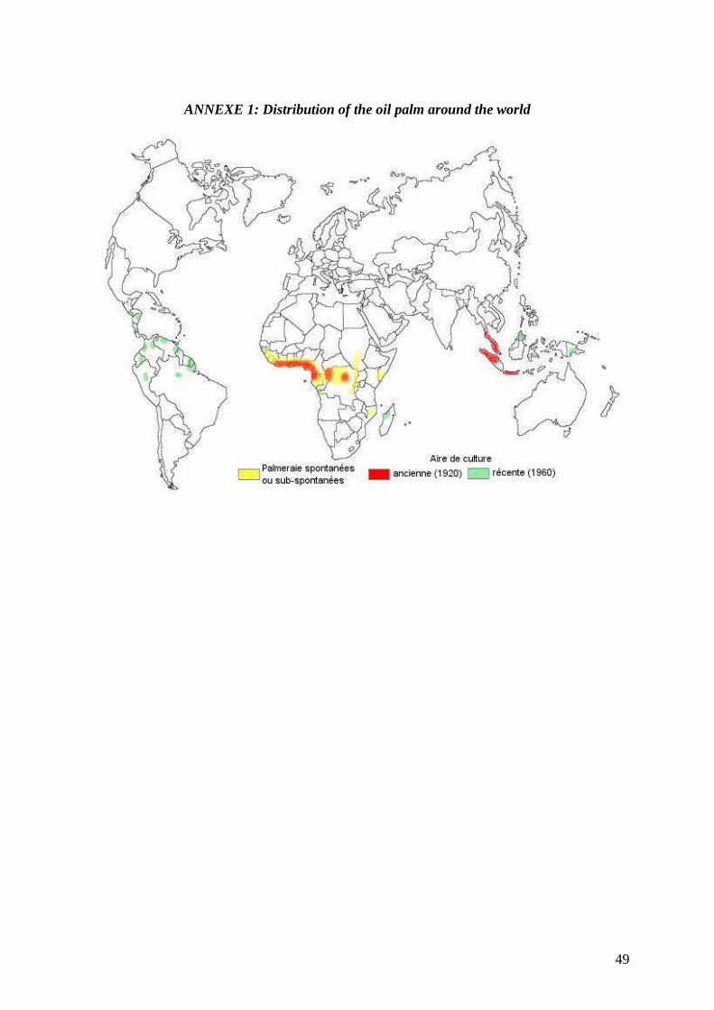
49

ANNEXE 1: Distribution of the oil palm around the world

50

ANNEXE 2: Data on the Asian oil palm cultivation

51

Numbers in million tons Source: USDA Foreign Agricultural Service, Production, Supply and distribution United States Department of Agriculture. www.fas.usda.gov

52

ANNEXE 3: Industrial Palm grove in multispectral mode (colour InfraRed)

53

ANNEXE 4 : Industrial palm oil in panchromatic mode

54

ANNEXE 5: List of all the tests achieved (SG combinations, databases…) The different databases are:

Database Palm-trees Description N°1 95 Soft deletion of abnormal spectra N°2 80 Deletion of any strange spectra N°3 80 Same than n°1 but without young palm-trees Final 95 Same than n°1 but justified skor corrections

Left: Four-class discrimination: Comparison between the use of original spectra and their logarithm

Right: Four-class discrimination: Comparison of two kinds of PLS coefficients for the PLS model:skor1=0.29 – skor2=0.6, and skor1=0.4 - skor2=0.6

55

Left: Four-class discrimination with PLS components 0.4 - 0.6 (also tested with 0.3 - 0.7)

Right: Three-class discrimination (without skor1) with PLS components 0.4 - 0.6 (also tested with 0.3 - 0.7)

56

Left: Two-classes discrimination with PLS components 0.4 - 0.6 (also tested with 0.3 - 0.7)

Right: Final tests on the final database

1