6th International Conference on Earthquake Geotechnical Engineering 1-4 November 2015 Christchurch, New Zealand

Prediction of Liquefaction Resistance Using a Combination of CPT

Cone and Sleeve Resistances - It’s really a Contour Surface

R. S. Olsen1

ABSTRACT

The Olsen method from 1980s and 1990s publications for prediction of liquefaction resistance was

developed using both CPT measurements. This method indirectly accounted for all soil types and relative strength consistencies without requiring the equivalent clean sand approach. A major update was achieved by minimizing conservative and unconservative outliers using two established databases. The final correlation was compared to other published methods.

Introduction

This paper re-introduces and updates the Olsen method for CPT-based prediction of liquefaction resistance from Olsen (1984), Olsen (1988), Olsen & Koester (1995), and Olsen (1997), using a graphic outlier based optimization techniques together with equation based outlier verification. I wrote this paper because about 10 engineers at the 10th U.S. National Conference on Earthquake Engineering in Anchorage (2014 July) asked me to update, as they said, the “Olsen method” for CPT prediction of liquefaction. Liquefaction Cyclic Resistance Ratio (CRR) is the liquefaction triggering resistance, namely liquefaction resistance (strength) divided by vertical effective stress. Normalized CRRM=7.5,σ’=1atm,α=1 in many publications will simply be shown as CRRe in this paper and the earthquake-induced normalized Cyclic Shear Stress Ratio (CSRM=7.5,σ’=1atm) will be shown as CSRe. All equations and plots in this paper use atmospheric pressure units (atm).

History

For almost 20 years the conventional approach for CPT based predicting of liquefaction resistance was to initially convert the normalized cone resistance (qc1) to equivalent clean sand normalized cone resistance (qc1Ncs) and then use it to predict CRRe (Boulanger & Idriss (2014)). The equivalent clean sand concept originated with Standard Penetration Test (SPT) liquefaction prediction in the early 1980s by H. Bolton Seed. Moss et al. (2006) summarized historic research efforts for a probability of liquefaction PL=15% to represent the conservative deterministic current practice: For reference, a predicted condition having PL=50% represents 50% probability of liquefaction triggering.

Databases The Olsen method was updated for this paper using two well-established CPT liquefaction

1USACE Senior Geotechnical Engineer, US Army Corps of Engineers (USACE), Headquarters USACE, Engineering & Construction Division (E&C), Washington DC, USA Richard.S.Olsen@usace.army.mil

databases: a) Moss et al. (2006), having data range represented as average ± one standard deviation, and b) updated data from Boulanger & Idriss (2014), having only average values. Both databases contain a large number of items but for this study only CPT measured values (qc1 and friction Ratio (Fr)), data quality index, liquefaction observation flag, and earthquake induced CSRe were required. The Moss et al. (2006) database consists of data ranging from very little data scatter to extremely large data scatter. For this study all the data in Boulanger & Idriss 2014) database was assumed to have a standard deviation data scatter equal to ±15% of the average. An important part of this study was to account for database data scatter. Data evaluation for this study used a working database range (to be described later) equal to 20% of the reported database scatter for each database point – this is the best means of specifically accounting for database points having large data scatter. Both databases also define each point with a quality index of A, B, or C (great, good, and old historic data). For this paper the quality index (Qf), to be defined later, will be assigned a quality multiplication index of 1.0, 0.7, and 0.3 for A, B, and C data levels.

The Olsen Method

Olsen (1984) published the first method of CPT predicted CRRe for soil types ranging from clean sands to clay, it was based on field observations of liquefaction and results from cyclic laboratory tests. The most recent version (Olsen & Koester (1995)) is shown as contours of CRRe on the CPT soil characterization chart (Log-log plot of qc1 versus Fr) in Figure 1a.

Figure 1. a) Olsen & Koester (1995) CPT prediction of CRRe, b) CRRe surface & Outliers

Updating the Olsen Method using Outliers The update in this paper was accomplished by minimizing outliers, namely the difference between database CSRe and a CPT predictive CRRe surface and defined by equation 1. CRRe lines in Figure 1a can be represented as a 3D CPT-predictive “CRRe contour surface” in Figure

1b. Database points of qc1, Fr, and CSRe together with the corresponding working database ranges (from the previous section) can be visually as boxes in Figure 1b. If the database box is below the CRRe surface, then the calculated predicted liquefaction factor of safety (F) is greater than 1. Outliers are defined as either a) Unconservative outlier (UO) when liquefaction is not predicted (F>1) to occur but field liquefaction was observed as illustrated by box U in Figure 1b, or b) Conservative Outliers (CO) when liquefaction is predicted (F<1) to occur but field liquefaction was not observed, as box C. The procedure was to move and reshape the CRRe surface contour to minimize the number of outliers and then reduce the magnitude of resulting outliers. Marginal anticipated behavior (M boxes) and anticipated behavior (A boxes) reflecting expected behavior and therefore cannot be used to improve the location of the CPT predictive CRRe surface. The conventional means of determining CRRe is shown in figure 2a as point D, which is the closest CRRe surface point to the closest corner of the database (point E). On a conventional 2D plot (qc1 versus Fr) CSRe and CRRe are both on the same Z line and therefore you won’t see a difference because both have same qc1 and Fr value. An alternative approach is to use the closest graphical point on the CRRe surface (point G) to the database corner (point E). Point G can be projected to point H on a qc1 versus Fr plot in figure 2a and point E projected to point F. The following discussion defines the PULL method. The resulting UO outlier vector from H to F is showing that if the CPT predictive CRRe surface is PULLED to the database box corner than this unconservative outlier will change to marginal anticipated behavior. The H to F vector in Figure 2a is represented in a qc1 versus Fr plot in Figure 2b, as well as other hypothetical PULL vectors and all pointing to closest CSRe box corners to achieve marginal anticipated behavior. The process for evaluating a given CPT predictive CRRe surface is to determine unconservative and conservative outliers PULL vectors for all points in the database then plot resulting vectors. The curve lookup software described in the appendix is required for this procedure.

Figure 2. a) Defining a 3D based UO outlier, b) 2D outliers illustrated for two CRRe levels

Outlier Optimization

Figure 3a shows the PULL outlier vectors using the Olsen (1988) CPT predicted CRRe surface. For this initial evaluation the number of PULL vectors is large and most are UO vectors. The idea is to reshape the predictive CRRe surface to final optimum shape by minimize the number (and magnitude) of outliers, and this is an iterative graphical process. Each iteration required generation of a new computer data file containing CRRe contour lines. Average unconservative and conservative outliers (Au and Ac) defined in equation 2 were used as an aid during the iteration process – minimizing Au and Ac but at the end insure Ac is larger than Au. After 21 major iterations which required re-digitization of all CRRe surface lines for each new data file, and many scale variations, the final CRRe surface and PULL vectors are shown in Figure 3b. 𝐷𝐷𝑆𝑆𝑆𝑆 = | 𝐶𝐶𝐶𝐶𝐶𝐶𝑒𝑒 − 𝐶𝐶𝐶𝐶𝐶𝐶𝑒𝑒| (1)

Au and Ac = ∑� � DSRCRRe

� 𝑄𝑄𝑓𝑓 �

𝑁𝑁𝑑𝑑𝑑𝑑 (2)

with CRRe = Closest graphically predictive point on CRRe surface (item G in Figure 2a) to database corner CSRe = Closest CSRe database corner (item E in Figure 2a) to the CRRe surface Qf = Quality index (less than 1, see text) for each database point reflecting A, B, or C data quality Ndb = Total number of items in database

Figure 3. Computer output of outlier “PULL” results; a) using Olsen (1988), b) final version The final CRRe surface in Figure 3b requires verification as to whether it meets the industry standard of predicting a probability of liquefaction PL=15%. The procedure employed was to

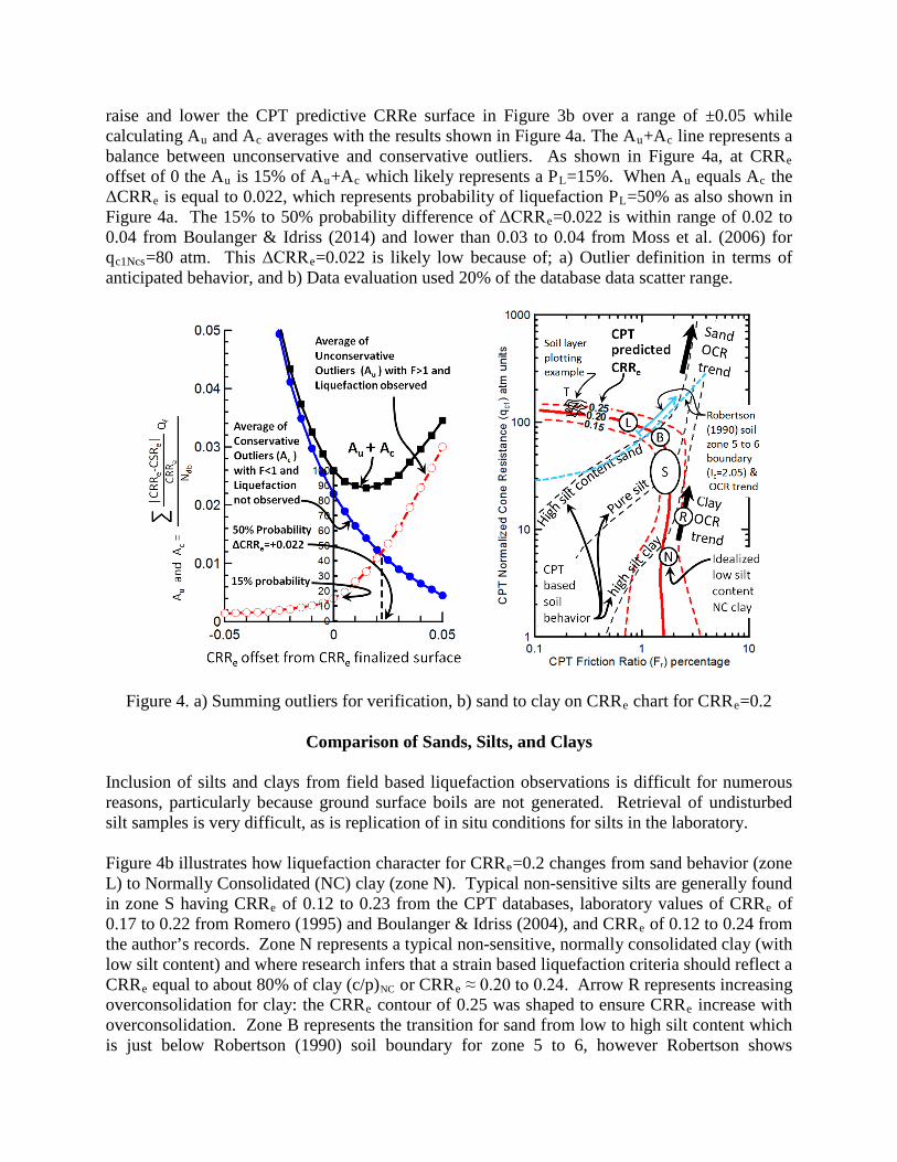
raise and lower the CPT predictive CRRe surface in Figure 3b over a range of ±0.05 while calculating Au and Ac averages with the results shown in Figure 4a. The Au+Ac line represents a balance between unconservative and conservative outliers. As shown in Figure 4a, at CRRe offset of 0 the Au is 15% of Au+Ac which likely represents a PL=15%. When Au equals Ac the ΔCRRe is equal to 0.022, which represents probability of liquefaction PL=50% as also shown in Figure 4a. The 15% to 50% probability difference of ΔCRRe=0.022 is within range of 0.02 to 0.04 from Boulanger & Idriss (2014) and lower than 0.03 to 0.04 from Moss et al. (2006) for qc1Ncs=80 atm. This ΔCRRe=0.022 is likely low because of; a) Outlier definition in terms of anticipated behavior, and b) Data evaluation used 20% of the database data scatter range.

Figure 4. a) Summing outliers for verification, b) sand to clay on CRRe chart for CRRe=0.2

Comparison of Sands, Silts, and Clays Inclusion of silts and clays from field based liquefaction observations is difficult for numerous reasons, particularly because ground surface boils are not generated. Retrieval of undisturbed silt samples is very difficult, as is replication of in situ conditions for silts in the laboratory. Figure 4b illustrates how liquefaction character for CRRe=0.2 changes from sand behavior (zone L) to Normally Consolidated (NC) clay (zone N). Typical non-sensitive silts are generally found in zone S having CRRe of 0.12 to 0.23 from the CPT databases, laboratory values of CRRe of 0.17 to 0.22 from Romero (1995) and Boulanger & Idriss (2004), and CRRe of 0.12 to 0.24 from the author’s records. Zone N represents a typical non-sensitive, normally consolidated clay (with low silt content) and where research infers that a strain based liquefaction criteria should reflect a CRRe equal to about 80% of clay (c/p)NC or CRRe ≈ 0.20 to 0.24. Arrow R represents increasing overconsolidation for clay: the CRRe contour of 0.25 was shaped to ensure CRRe increase with overconsolidation. Zone B represents the transition for sand from low to high silt content which is just below Robertson (1990) soil boundary for zone 5 to 6, however Robertson shows

increasing OCR starting at CRRe=0.18 (which is unlikely). Zone B will be shown later to have the same predictive CRRe=0.2 for several other methods. The CRRe=0.2 contour trending, for non clean sands, should go through the middle of zone B, through zone S, and left of zone N, all for normally consolidated conditions.

Final CRRe Contour Surface and Comparison to other Methods The final CPT-predicted CRRe relationship is shown in Figure 5a for the standardized predicted liquefaction probability PL=15%. This method allows field project data to be plotted (for example item T in figure 4b) and directly compared to CRRe contours.

Figure 5. a) Final CPT predicted CRRe surface, b) CRRe surfaces for all methods Figure 5b compares the final CRRe contour surface to that of the Moss, et al. (2006) and Boulanger & Idriss (2014) methods. Both of these other methods use complex equations and some form of the equivalent clean sand approach. Both methods were converted to graphic contours using an iterative software routine developed during this study - this is the first time all three methods could be directly compared. The Moss, et al. (2006) method for CRRe=0.1 and CRRe=0.2 shows a very simple curve despite the complex equations. Boulanger & Idriss (2014) method for CRRe=0.2 shows a curious bend at Fr=0.8% and interesting behavior for CRRe=0.1 at low Fr (there are apparently two CRRe=0.1 curves). Neither of these other methods limit CRRe prediction for high Fr (specifically, Fr greater than 2% represents high OCR silts/clays), nor do they show any CRRe deviation from high silt content sand (zone B) toward silt behavior

(zone S) – the Boulanger & Idriss CRRe=0.2 contour at point B is almost a mirror image of the final contour for this paper. All three methods have similar CRRe values at two zone locations on the soil characterization chart; a) point B for CRRe=0.2 at qc1=85 atm Fr=1.4%, and b) point W for CRRe=0.1 at qc1=50 atm Fr=0.25%; this is likely because all three methods use the same database from 2006. The Moss, et al (2006) and Boulanger & Idriss (2014) methods both use high data scatter correlations of predicted fines content based on CPT soil type (Ic) for the equivalent clean sand approach, also known as “fines adjustment.” Both methods then use the resulting equivalent clean sand cone resistance (qc1Ncs) to correlate to liquefaction resistance (same as the SPT based approach from the 1980s). These two methods also do not account for database range and it is unclear how database quality is accounted. From the results in Figure 5b, the equation based clean sand approach is not producing realistic predicted liquefaction results.

Conclusions The Olsen method for CPT-based prediction of liquefaction for sands to clay was updated using graphic and equation based outlier optimization techniques. The resulting contour surface on the CPT soil characterization chart (log-log plot of qc1 versus Fr) is too complex to be represented with complex equations and therefore requires the curve lookup software procedure described in the Appendix. The final contour of CRRe allows practicing engineers (as well as researchers) to properly visualize liquefaction trends and allow field data to be plotted and directly compared to CRRe contours. Special software was developed that allowed the Boulanger & Idriss (2014) and Moss et al. (2006) predicted liquefaction resistance to be plotted on the CPT soil characterization chart and directly compared to the Olsen method. Both of these other methods were based on complex equations, but the very simple plotted shapes that they produce do not match existing data for soils ranging from silts to clay. The CPT equivalent clean sand approach has clouded technical advancement, because errors are introduced as equations are developed both to predict qc1Ncs as well as CRRe. These methods cannot account for the dramatic CRRe changes observed as soil type varies from clean sand to silt to clay. Complex equations for prediction of liquefaction and use of the equivalent clean sand approach may be unwarranted; their continued use is a subject for future discourse.

Acknowledgments

This paper does not reflect recommendations, endorsement, or policy of the U.S. Army Corps of Engineers. I thank Dr. Joe Koester review of this paper. The paper was initially submitted for conference review on 2015 March 1. Full size images are posted at 6iCEGE.geostaff.net

References

Boulanger, R.W., Idriss, I.M (2014). “CPT and SPT based Liquefaction Triggering Procedures.” UC Davis Center for Geotechnical modeling, Report No UCD/CGM-14/01

Boulanger, R.W., Idriss, I.M (2004). “Evaluating the Potential for Liquefaction or Cyclic Failure of Silts and

Clays.” UC Davis Center for Geotechnical modeling, Report No UCD/CGM-04/01

Moss, R. E. S., Seed, R. B., Kayen, R. E., Stewart, J. P., Kiureghian, and Cetin (2006). "CPT-Based Probabilistic and Deterministic Assessment of In Situ Seismic Soil Liquefaction Potential" Journal of Geotechnical And Geoenvironmental Engineering, ASCE, Aug 2006.

Olsen, R. S. (1984). “Liquefaction analysis using the cone penetrometer test.” Proc., 8th World Conf. on Earthquake Engineering EERI, San Francisco. Olsen, R. S., and Koester, J. P. (1995). “Prediction of liquefaction resistance using the CPT.” Proc., Int. Symp. on Cone Penetration Testing, CPT 95, Linkoping, Sweden. Olsen, R. S. (1997). "Cyclic liquefaction based on the cone penetrometer test." NCEER Workshop on Evaluation of Soil Liquefaction, NCEE, Report No. NCEER-97-0022, pp. 225–76.

Robertson, P.K. (1990). "Soil classification using the cone penetration test." Canadian Geotech. J., 27(1)

Robertson, P. K. (2009). "Interpretation of cone penetration tests.” Canadian Geotech. J., 46: 1337-1355 Romero, S. (1995). The behavior of silt as clay content is increased. MS thesis, Univ. of Cal. at Davis.

Appendix This section describes how to develop software for the curve lookup procedure. The first step is to extend all predictive contours beyond chart limits, shown as B-E lines in Figure 6a, ensuring that contour ends are beyond the adjacent contour intersections (C lines). Determine curve lookup method: either XyC or YxC. The XyC approach cannot be used for R curves in figure 6b because for a given X value there are two contour intersection shown as T points. For the XyC procedure each line in Figure 6c is evaluated. For the given X value the Points E and F can be found for each line. S points and corresponding y values (i.e. yC1, yC2, yC3, etc) are determined using linear calculations based on points E and F and given X. S points are evaluated until it bounds the given Y, in this case yC2 and yC3. The curve value Cp is calculated using linear interpolation based on given Y, points yC2 and yC3, and curves values C2 and C3.

Figure 6. Steps for Curve Lookup software coding, a) Setup, b) Method selection, c) Procedure