Prediction of ground reaction forces and moments

during sports-related movements

Sebastian Laigaard Skals

Master’s Thesis submitted 2nd June 2015

Master of Sports Technology

Department of Health Science and Technology

Aalborg University

Supervisors

Michael Skipper Andersen

Miguel Nobre Castro

1

Prediction of ground reaction forces and

moments during sports-related movements

Sebastian Laigaard Skals

Department of Health Science and Technology, Aalborg University, Aalborg, Denmark

Abstract

Inverse dynamic analysis (IDA) on musculoskeletal models has become a commonly used method to study

human movement. However, when solving the inverse dynamics problem, inaccuracies in experimental

input data and a mismatch between model and subject leads to dynamic inconsistency. By predicting the

ground reaction forces and moments (GRF&Ms), this inconsistency can be reduced and force plate

measurements become unnecessary. In this study, a method for predicting the GRF&Ms was adopted and

validated for an array of sports-related movements. The method uses a scaled musculoskeletal model and

the equations of motion alone to predict GRF&Ms from full-body motion, and entails a dynamic contact

model and optimization techniques to solve the indeterminacy during double support. The method was

applied to ten healthy subjects performing e.g. running, a side-cut manoeuvre and vertical jump. Pearson’s

correlation coefficient (r) was used to compare the predicted GRF&Ms and associated joint kinetics to the

corresponding variables obtained from a traditional IDA approach, where the GRF&Ms were measured

using force plates. In addition, peak vertical GRFs and resultant JRFs were computed and statistically

compared. The main findings were that the method provided estimates comparable to the traditional IDA

approach for vertical GRFs (r ranging from 0.96 to 0.99, median 0.99), joint flexion moments (r ranging from

0.79 to 0.98, median 0.93) and resultant JRFs (r ranging from 0.78 to 0.99, median 0.97), across all

movements. Although discrepancies were identified for some variables and the majority of the peak forces

were significantly different, the former were mainly contributed to noise while the differences in peak

forces could potentially be overcome by adjusting parameters in the contact model. Considering these

results, this method could be used instead of force plate data, hereby facilitating IDA in sports science

research and providing valuable opportunities for complete IDA using motion analysis systems that does

not commonly incorporate force plate data, such as marker-less motion capture.

Keywords: Ground reaction forces and moments, musculoskeletal model, inverse dynamics, sports-related

movements, validation

2

1. Introduction

Musculoskeletal modelling is an important tool towards understanding the internal mechanisms of the

body during various movements and loading conditions, which are otherwise impractical or impossible to

measure. To this day, it remains very challenging to measure muscle, ligament and joint forces in vivo and

the associated procedures are invasive. Therefore, the use of simulation models to estimate these variables

has become widespread and contribute important information to a variety of scientific fields, such as

clinical gait analysis (Zajac et al., 2003; Vaughan et al., 1999), ergonomics (Rasmussen et al., 2003a, 2003b),

orthopaedics (Mellon et al., 2013, 2015; Weber et al., 2014) and sports biomechanics (Payton and Bartlett,

2008).

There exist a number of different analytical approaches within the area of musculoskeletal

modelling. Firstly, Forward Dynamics-based tracking methods use computed muscle control, which is held

up against measured kinematics to determine the muscle actions that produce a given motion (Thelen and

Anderson, 2006). Secondly, EMG-driven forward dynamics estimates the contribution of individual muscles

during motion using a combination of kinematic and electromyographic data (Barret et al., 2007). Thirdly,

Dynamic Optimization involves defining the goal of the motor task and applying an optimization approach

to compute the motor patterns and kinematics (Anderson and Pandy, 2001). Finally, Inverse Dynamics

approaches the problem from the opposite end and determines the muscle and joint forces from kinematic

and/or external force data (Erdemir et al., 2007; Damsgaard et al., 2006). More specifically, measurements

of body motion and external forces are input to the equations of motion and the joint reaction and muscle

forces can be computed in a process known as muscle recruitment (Damsgaard et al., 2006; Rasmussen et

al., 2001).

Typically, marker-based motion analysis and force plate measurements are used to determine body

segment kinematics (i.e., positions, velocities and accelerations) (Andersen et al., 2009; Cappozzo et al.,

2005) and ground reaction forces and moments (GRF&Ms) (Nigg, 2006), respectively, while the body

segment parameters (i.e., segment mass, centre-of-mass and moment-of-inertia) are determined through

cadaver-based studies (Carbone et al., 2015; Horsman et al., 2007; Clauser et al., 1969) and model scaling

techniques (Lund et al., 2015; Andersen et al., 2010). However, it is well-known that the results of inverse

dynamic analysis (IDA) are sensitive to inaccuracies in these input data (Pámies-Vila et al., 2012; Riemer et

al., 2008). Inaccuracies can stem from multiple sources, such as estimating joint (Schwartz et al., 2005) and

body segment parameters (Rao et al., 2006; Pearsall and Costigan, 1999), marker sliding relative to the

underlying bone due to soft tissue artefacts (Leardini et al., 2005; Stagni et al., 2005), marker misplacement

(Della Croce et al., 2005), camera-system (Chiari et al., 2005) and force plate calibration (Collins et al.,

3

2009), determining centre-of-pressure (Middleton et al., 1999) and variability in force plate data

(Psycharakis and Miller, 2006). In addition, there exists a fundamental mismatch between the

measurements obtained from the real biosystem and the mathematical model used for analysis (Hatze,

2002). When analysing full-body models, the system becomes over-determinate as the GRF&Ms are input

to the equations of motion (Cahouët et al., 2002; Hatze, 2002; Kuo, 1998). In some cases, it can be

justifiable to solve the overdeterminacy by simply discarding acceleration measurements for one or more

segments in the model. When this is not possible, however, the dynamic inconsistency arising from system

overdeterminacy and experimental input inaccuracies can be solved by introducing residual forces and

moments in the model to obtain dynamic equilibrium (Fluit et al., 2014a; Cahouët et al., 2002; Kuo, 1998).

In order to improve dynamic consistency, these residual forces and moments have been used to

reduce error effects from the input data through various optimization methods (Riemer and Hsiao-

Wecksler, 2008; Delp et al., 2007; Cahouët et al., 2002; Kuo, 1998; Vaughan et al., 1982). Alternatively,

dynamic consistency can be improved by deriving the GRF&Ms from the model kinematics and segment

dynamical properties only, which is commonly known as the top-down approach (Riemer and Hsiao-

Wecksler, 2008; Cahouët et al., 2002). The application of the top-down approach has traditionally been

limited by the fact that the inverse dynamics problem becomes indeterminate during double contact

phases, where the system forms a closed kinetic chain (Fluit et al., 2014a; Audu et al., 2007). In recent

years, however, several studies have provided solutions to this issue (Fluit et al., 2014a; Choi et al., 2013;

Eel Oh et al., 2013; Robert et al., 2013; Ren et al., 2008; Audu et al., 2007; Audu et al., 2003). Most recently,

Fluit et al. (2014a) demonstrated a universal method for predicting GRF&Ms using kinematic data and a

scaled musculoskeletal model only. The indeterminacy issue during double contact was solved by

employing a dynamic contact model and optimization techniques. Specifically, the researchers introduced

five artificial muscle-like actuators at 12 contact points under each foot in the model and computed the

GRF&Ms as part of the muscle recruitment algorithm. The method was validated against measured data for

an array of activities of daily living, such as gait, deep squatting and stair ascent, and reasonably good

results were obtained for all analysed activities.

Besides improving dynamic consistency, predicting rather than measuring GRF&Ms obviates the

need for force plate measurements, which has some additional advantages. 1) The measurement errors

associated with force plates can be eliminated. 2) Force plate targeting can be avoided; an issue that may

affect the resulting segment angles and GRF&Ms (Challis, 2001). 3) It facilitates IDA of movements that are

continuous and occupy a large space (Choi et al., 2013). 4) GRF&Ms can be obtained in outdoor

environments without having to instrument force plates. Currently, motion analysis systems exist that are

4

able to operate in outdoor environments, but force plates are difficult and expensive to install in multi-

settings (Choi et al., 2013) and are sensitive to temperature and humidity variations (Psycharakis and

Miller, 2006). For sports science research, 3 and 4 are particularly advantageous. Ensuring force plate

impact during motions that are highly dynamic and require large amounts of space can be difficult, which is

the case for many movements associated with sports. This can potentially restrict natural execution of the

motion or even require force plate targeting to ensure impact, which could compromise the quality of the

measurements. In addition, many sports-related movements can only be analysed in their entirety by

performing measurements outdoors, which is currently infeasible using force plates. However, none of the

existing methods for predicting GRF&Ms have been validated for sports-related movements.

Therefore, the goal of this study was to evaluate the accuracy of the method proposed by Fluit et al.

(2014a) to predict GRF&Ms during sports-related movements. This was accomplished by performing IDA on

a variety of movements, such as running, vertical jump and a side-cut manoeuvre. For validation, the

predicted GRF&Ms and associated joint kinetics were compared with the corresponding values from the

model, in which GRF&Ms were obtained using force plates. If comparable accuracy between these two

methods can be established, it would provide new and valuable opportunities for IDA in sports science

research.

2. Materials and methods

2.1 Experimental procedures

Ten healthy subjects (8 males and 2 females, age: 25.70 ± 1.49 years, height: 180.80 ± 7.39 cm, weight:

76.88 ± 10.37 kg) volunteered to participate in the study and provided written informed consent. The study

was conducted at the Department of Health Science and Technology, Aalborg University, Aalborg,

Denmark.

During measurements, male subjects exclusively wore tight fitting underwear or running tights, while

female subjects also wore a sports-brassiere. In addition, all subjects wore a pair of running shoes in their

preferred size, specifically the Brooks Ravenna 2 (Brooks Sports Inc., Seattle, WA, US). This decision was

made in order to minimize discomfort and, hereby, facilitate a more natural execution of the movements.

Initially, a 5 min warm-up at 160 W was completed on a cycle ergometer before multiple practice trials

were performed. The practice trials served two overall purposes and were preceded by a thorough

instruction. First, some of the included movements were considered technically challenging and required

multiple repetitions to ensure consistent technique throughout the duration of the experiment.

5

Furthermore, it was desired to obtain some degree of technical consistency between subjects to reduce

variability in the resulting measurements. Second, the starting position for each movement was established

through trial-and-error until the subjects were able to consistently impact the force plates. When it was

assessed that the subjects were consistently able to perform the movements with adequate technique and

impact the force plates accurately, their starting position was marked and they were given a brief pause

before markers were taped to their skin.

The following movements were included in the study: 1) Running at a comfortable pace, 2)

backwards running, 3) a side-cut manoeuvre, 4) vertical jump, and 5) accelerating from a standing position

(ASP), imitating the initiation of running. These movements were chosen, as they represent some of the

most common movements associated with sports and can be performed without specialised skills. In

addition, the movements provided varied characteristics in the resulting GRF&Ms, considering factors such

as force plate impact time, force magnitude and direction as well as providing single and double contact

phases. Initially, all running trials were completed. Subjects were instructed to run at a comfortable self-

selected pace and impact the force plate with their right foot, aimed towards facilitating a natural running

style and a consistent pace between trials. For the side-cut manoeuvre, subjects were instructed to

perform a slowly paced run-up, impact the centre of the force plate with their right foot, and accelerate to

their left-hand side while targeting a cone. The centre of the force plate was marked with white tape and

the cone was placed 2 m from the tape mark, angled at 45 degrees from the initial running direction.

Backwards running was executed at a self-selected pace and the subjects had to impact the force plate with

their right foot. During practice trials, the starting position had been established where the subjects were

able to impact the force plate accurately and consistently. As a result, the subjects only had to focus on

executing the movement with consistent technique, while keeping their focus straight ahead, i.e., away

from the running direction, during measurements. Vertical jump was performed as a counter-movement

jump, initiated with the subjects standing with each foot on separate force plates. They were asked to keep

their hands fixated on the hips, focus straight ahead for the entirety of the movement cycle and refrain

from excessive hip flexion. While complying with these constraints, they were asked to push-off with their

legs at maximal capacity and attempt to achieve their maximal jump height. Finally, ASP was initiated with

the subjects’ feet separated in the sagittal plane and placed on separate force plates, while their arms were

positioned inversely to their feet, closely resembling a natural initiation of running. From this position, they

were asked to accelerate to their comfortable running pace. Five trials were completed for all movements,

each consisting of one full movement cycle. Videos showing the executions of each movement are provided

as supplementary material (Sup. Video 1-5).

6

2.2 Data collection

A total of 35 reflective markers were placed on the subjects, consisting of 29 markers placed on the skin

surface and three markers placed on each running shoe, resembling the position of the first and fifth

metatarsal and the top of the calcaneus bone. No markers were placed on the head. Further details

regarding the marker protocol are provided as appendix. Marker trajectories were tracked using a marker-

based motion capture system, consisting of eight infrared high-speed cameras (Oqus 300 series), sampling

at 250 Hz, combined with Qualisys Track Manager v. 2.9 (Qualisys, Gothenburg, Sweden). GRF&Ms were

obtained at 2000 Hz using two force plates (width/length = 464/508 mm) (Advanced Mechanical

Technology, Inc., Watertown, MA, US), which were embedded in the laboratory floor.

2.3 Data processing

3-D marker trajectories and force plate data were low-pass filtered using second order, zero-phase

Butterworth filters with a cut-off frequency of 15 and 10 Hz, respectively. For all movements, three of the

five successful trials were included for further analysis, yielding a total of 150 trials used to validate the

predicted GRF&Ms and the associated joint kinetics. Trials were excluded due to occasional marker

occlusion or inadequate impact of the force plates, i.e., the whole foot was not in complete contact or the

impact occurred too close to the edges of the force plate surface.

2.4 Prediction of GRF&Ms

The prediction of GRF&Ms was enabled by partly adopting the method of Fluit et al. (2014a). However,

some key alterations where made to the method, which are specified in the following. The GRF&Ms were

predicted by creating five artificial muscle-like actuators at 18 contact points defined under each foot of the

musculoskeletal model (Figure 1). In order to compensate for the sole thickness of the running shoes and

the soft tissue under the heel, the contact points on the heel were offset by 35 mm and all other points

offset by 25 mm from the model bone geometry. Of the five actuators, one actuator was aligned with the

vertical axis of the force plates (Z-axis) and generated a normal force. The other actuators were defined in

two pairs that were aligned with the medio-lateral (X-axis) and antero-posterior axis (Y-axis) of the force

plates, and were able to generate positive and negative static friction forces (with a friction coefficient of

0.5).

To establish ground contact, a dynamic contact model was applied to determine the activation level

of each actuator. This approach ensured that each actuator would only generate a contact force if their

associated contact point, p, was sufficiently close to the floor and almost without motion. The maximal

strength of each actuator was set to 𝐹𝑚𝑎𝑥 = 0.4 𝐵𝑊, the activation threshold distance from p to the

7

ground plane was set to 𝑧𝑙𝑖𝑚𝑖𝑡 = −0.01 𝑚, and the activation threshold velocity of p was set to 𝑣𝑙𝑖𝑚𝑖𝑡 =

1.3 𝑚/𝑠. In order to be activated, each contact point had to overlap with a user-defined artificial ground

plane in the model environment, as illustrated in Figure 1. The specified distance, 𝑧𝑙𝑖𝑚𝑖𝑡, represent the

location of the artificial ground plane relative to the origin of the global reference frame and not the actual

location of the ground. To determine the strength profile of each contact point, a nonlinear strength

function was defined as

𝑐𝑝,𝑖 = {

𝐹𝑚𝑎𝑥 𝐹𝑠𝑚𝑜𝑜𝑡ℎ

0

𝑖𝑓 𝑧𝑟𝑎𝑡𝑖𝑜 ≤ 0.8 𝑎𝑛𝑑 𝑣𝑟𝑎𝑡𝑖𝑜 ≤ 0.15 𝑖𝑓 0.8 ≤ 𝑧𝑟𝑎𝑡𝑖𝑜 < 1 𝑎𝑛𝑑 0.15 ≤ 𝑣𝑟𝑎𝑡𝑖𝑜 < 1 (1) 𝑜𝑡ℎ𝑒𝑟𝑤𝑖𝑠𝑒

𝑤ℎ𝑒𝑟𝑒 𝑧𝑟𝑎𝑡𝑖𝑜 =𝑝𝑧

𝑧𝑙𝑖𝑚𝑖𝑡

𝑎𝑛𝑑 𝑣𝑟𝑎𝑡𝑖𝑜 =

𝑝𝑣𝑒𝑙

𝑣𝑙𝑖𝑚𝑖𝑡

where 𝑝𝑧 and 𝑝𝑣𝑒𝑙 defined the height and velocity of each contact point relative to the ground,

respectively. Eq. (1) specifies that each actuator would assume the strength 𝐹𝑚𝑎𝑥 if the associated p

reached 𝑧𝑙𝑖𝑚𝑖𝑡 and 𝑣𝑙𝑖𝑚𝑖𝑡. However, in order to prevent discontinuities in the predicted GRF&Ms due to the

sudden transition of p from inactive to fully active, a smoothing function was defined as

𝐹𝑠𝑚𝑜𝑜𝑡ℎ = 𝐹𝑚𝑎𝑥 𝑧𝑠𝑚𝑜𝑜𝑡ℎ𝑣𝑠𝑚𝑜𝑜𝑡ℎ (2)

Figure 1 – Location of the contact points under the foot of the musculoskeletal model (top left), side-view of the contact points

specifying the offset distances (bottom left) and the point activation after established ground contact (right).

8

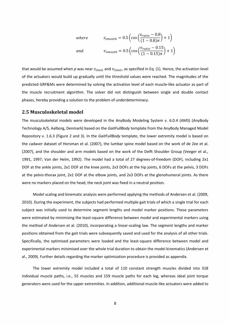
𝑤ℎ𝑒𝑟𝑒 𝑧𝑠𝑚𝑜𝑜𝑡ℎ = 0.5 (cos (

𝑧𝑟𝑎𝑡𝑖𝑜 − 0.8

(1 − 0.8)𝜋) + 1)

𝑎𝑛𝑑 𝑣𝑠𝑚𝑜𝑜𝑡ℎ = 0.5 (cos (

𝑣𝑟𝑎𝑡𝑖𝑜 − 0.15

(1 − 0.15)𝜋) + 1)

that would be assumed when p was near 𝑧𝑙𝑖𝑚𝑖𝑡 and 𝑣𝑙𝑖𝑚𝑖𝑡, as specified in Eq. (1). Hence, the activation level

of the actuators would build up gradually until the threshold values were reached. The magnitudes of the

predicted GRF&Ms were determined by solving the activation level of each muscle-like actuator as part of

the muscle recruitment algorithm. The solver did not distinguish between single and double contact

phases, hereby providing a solution to the problem of underdeterminacy.

2.5 Musculoskeletal model

The musculoskeletal models were developed in the AnyBody Modeling System v. 6.0.4 (AMS) (AnyBody

Technology A/S, Aalborg, Denmark) based on the GaitFullBody template from the AnyBody Managed Model

Repository v. 1.6.3 (Figure 2 and 3). In the GaitFullBody template, the lower extremity model is based on

the cadaver dataset of Horsman et al. (2007), the lumbar spine model based on the work of de Zee et al.

(2007), and the shoulder and arm models based on the work of the Delft Shoulder Group (Veeger et al.,

1991, 1997; Van der Helm, 1992). The model had a total of 27 degrees-of-freedom (DOF), including 2x1

DOF at the ankle joints, 2x1 DOF at the knee joints, 2x3 DOFs at the hip joints, 6 DOFs at the pelvis, 3 DOFs

at the pelvis-thorax joint, 2x1 DOF at the elbow joints, and 2x3 DOFs at the glenohumeral joints. As there

were no markers placed on the head, the neck joint was fixed in a neutral position.

Model scaling and kinematic analysis were performed applying the methods of Andersen et al. (2009,

2010). During the experiment, the subjects had performed multiple gait trials of which a single trial for each

subject was initially used to determine segment lengths and model marker positions. These parameters

were estimated by minimising the least-square difference between model and experimental markers using

the method of Andersen et al. (2010), incorporating a linear-scaling law. The segment lengths and marker

positions obtained from the gait trials were subsequently saved and used for the analysis of all other trials.

Specifically, the optimised parameters were loaded and the least-square difference between model and

experimental markers minimised over the whole trial duration to obtain the model kinematics (Andersen et

al., 2009). Further details regarding the marker optimization procedure is provided as appendix.

The lower extremity model included a total of 110 constant strength muscles divided into 318

individual muscle paths, i.e., 55 muscles and 159 muscle paths for each leg, whereas ideal joint torque

generators were used for the upper extremities. In addition, additional muscle-like actuators were added to

9

the origin of the pelvis segment, which were able to generate residual forces and moments up to 10 N or

Nm. The activation levels of these muscles were solved as part of the muscle recruitment, aimed towards

minimizing their contribution. This approach was utilized in order to improve numerical stability. The

muscle recruitment problem was solved by minimizing the sum of the squared muscle activities (the ratio

between muscle forces and maximal isometric strengths), also known as Quadratic muscle recruitment,

hereby, providing the muscle forces and thus the predicted GRF&Ms. The skeletal muscles and muscle-like

Figure 2 – Musculoskeletal models of a subject performing running (left), backwards running (centre) and a side-cut manoeuvre

(right).

Figure 3 – From left to right: Musculoskeletal models of a subject performing ASP (initiation of the movement and near toe-off)

and vertical jump (counter-movement and past toe-off).

10

actuators were weighted equally during recruitment, but the strength of the actuators associated with the

GRF&Ms were high compared to the skeletal muscles, whereas the strength of the residuals were relatively

low.

2.6 Data analysis

For the running, backwards running and side-cut trials, data were analysed from the first foot-force plate

contact instant to the last frame of contact. Vertical jump trials were analysed in the 800 ms up till toe-off,

which included the complete counter-movement cycle. ASP trials were analysed in the 600 ms up till toe-

off of the rear foot. The following variables were included in the analysis: Antero-posterior ground reaction

force (GRF), medio-lateral GRF, vertical GRF, sagittal ground reaction moment (GRM), frontal GRM,

transverse GRM, ankle flexion moment (AFM), knee flexion moment (KFM), hip flexion moment (HFM), hip

abduction moment (HAM), hip external rotation moment (HERM), ankle resultant joint reaction force (JRF),

knee resultant JRF and hip resultant JRF. In addition, peak resultant JRF for the ankle, knee and hip, and

peak vertical GRF were computed. For the running, backwards running and side-cut trials, the selected

variables were analysed for the right leg only, i.e., the stance phases of the movement cycles. For the

vertical jump and ASP trials, the variables were analysed for the right and left leg separately.

In order to assess the accuracy of the predicted GRF&Ms and the associated joint kinetics, these data

were compared to the corresponding variables in the model where the GRF&Ms were obtained through

force plate measurements. Pearson’s correlation coefficient (r) and root-mean-square deviation (RMSD)

were computed to compare the selected variables. Following the procedures of Taylor (1990), the absolute

values of r were categorized as weak, moderate, strong and excellent for r ≤ 0.35, 0.35 < r ≤ 0.67, 0.67 < r

≤ 0.90, 0.90 < r, respectively. To test the differences between the computed peak GRFs and peak resultant

JRFs associated with each approach, Wilcoxon paired-sample tests were applied for which p < 0.05 are

reported as a significant difference.

3. Results

The time-histories of the selected variables for running, backwards running and side-cut are depicted in

Figures 4-7 (a), and vertical jump and ASP trials are depicted in Figures 4-7 (b). The results of the statistical

analysis and the RMSD for running, backwards running, and side-cut are summarized in Tables 1-3 (a), while

the results for vertical jump and ASP are summarized in Tables 1-3 (b). For the majority of the variables,

comparable results were observed between datasets. Across all movements, excellent correlations were

found for vertical GRF (r ranging from 0.96 to 0.99, median 0.99), and strong to excellent correlations were

found for sagittal GRM (r ranging from 0.69 to 0.95, median 0.87), all joint flexion moments (r ranging from

11

Figure 4 (a) – Results for running, backwards running and side-cut, illustrating antero-posterior GRF, medio-lateral GRF and

vertical GRF. The predicted variables are illustrated in blue and the measured variables in red. The results are presented as the

mean ± 1 SD (shaded area).

Figure 4 (b) – Results for vertical jump and accelerate from standing position (ASP), illustrating antero-posterior GRF, medio-

lateral GRF and vertical GRF. The predicted variables are illustrated in blue and the measured variables in red. The results are

presented as the mean ± 1 SD (shaded area).

12

Figure 5 (a) – Results for running, backwards running and side-cut, illustrating frontal GRM, sagittal GRM and transverse GRM.

The predicted variables are illustrated in blue and the measured variables in red. The results are presented as the mean ± 1 SD

(shaded area).

Figure 5 (b) – Results for vertical jump and accelerate from standing position (ASP), illustrating frontal GRM, sagittal GRM and

transverse GRM. The predicted variables are illustrated in blue and the measured variables in red. The results are presented as

the mean ± 1 SD (shaded area).

13

0.79 to 0.98, median 0.93) and resultant JRFs (r ranging from 0.78 to 0.99, median 0.97). The variables

showing the largest discrepancies between the two datasets were transverse GRM (r ranging from -0.19 to

0.86, median 0.09), frontal GRM (r ranging from 0.39 to 0.96, median 0.59) and medio-lateral GRF (r

ranging from 0.12 to 0.96, median 0.61). The model consistently overestimated the computed peak forces

with the only clear exceptions being the resultant JRFs for the right leg (RL) during ASP, which were

consistently underestimated, the ankle peak resultant JRF during side-cut, and peak vertical GRFs for the RL

and left leg (LL) during ASP, which showed similar values. The Wilcoxon-paired sample tests showed

significant differences for all peak forces, except ankle peak resultant JRF during side-cut (p = 0.64) and

peak vertical GRF for the RL (p = 0.10) and LL (p = 0.07) during ASP. The results for each movement are

summarized in the following.

Figure 6 (a) – Results for running, backwards running and side-cut, illustrating ankle (AFM), knee (KFM) and hip flexion moment

(HFM), hip abduction moment (HAM) and hip external rotation moment (HERM). The variables associated with the predicted

and measured GRF&Ms are illustrated in blue and red, respectively. The results are presented as the mean ± 1 SD (shaded area).

14

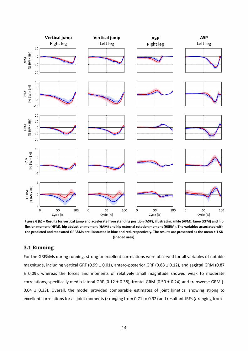
3.1 Running

For the GRF&Ms during running, strong to excellent correlations were observed for all variables of notable

magnitude, including vertical GRF (0.99 ± 0.01), antero-posterior GRF (0.88 ± 0.12), and sagittal GRM (0.87

± 0.09), whereas the forces and moments of relatively small magnitude showed weak to moderate

correlations, specifically medio-lateral GRF (0.12 ± 0.38), frontal GRM (0.50 ± 0.24) and transverse GRM (-

0.04 ± 0.33). Overall, the model provided comparable estimates of joint kinetics, showing strong to

excellent correlations for all joint moments (r ranging from 0.71 to 0.92) and resultant JRFs (r ranging from

Figure 6 (b) – Results for vertical jump and accelerate from standing position (ASP), illustrating ankle (AFM), knee (KFM) and hip

flexion moment (HFM), hip abduction moment (HAM) and hip external rotation moment (HERM). The variables associated with

the predicted and measured GRF&Ms are illustrated in blue and red, respectively. The results are presented as the mean ± 1 SD

(shaded area).

15

Figure 7 (a) – Results for running, backwards running and side-cut, illustrating the ankle, knee and hip resultant JRFs. The

variables associated with the predicted and measured GRF&Ms are illustrated in blue and red, respectively. The results are

presented as the mean ± 1 SD (shaded area).

Figure 7 (b) – Results for vertical jump and accelerate from standing position (ASP), illustrating the ankle, knee and hip resultant

JRFs. The variables associated with the predicted and measured GRF&Ms are illustrated in blue and red, respectively. The results

are presented as the mean ± 1 SD (shaded area).

16

Table 1 (a) – RMSD for the selected variables during running, backwards running and side-cut. The results are presented as the mean ± 1 SD.

Variable Running Backwards running Side-cut

Anterior-posterior GRF (N/kg) 7.86 ± 3.55 6.73 ± 1.37 13.04 ± 4.02

Medio-lateral GRF (N/kg) 5.61 ± 1.48 4.62 ± 1.27 8.56 ± 1.60

Vertical GRF (N/kg) 15.66 ± 3.49 12.59 ± 3.57 17.11 ± 4.08

Frontal GRM (Nm/kg) 1.75 ± 0.43 1.61 ± 0.43 1.65 ± 0.50

Sagittal GRM (Nm/kg) 3.60 ± 1.50 2.95 ± 1.00 3.46 ± 0.95

Transverse GRM (Nm/kg) 1.17 ± 0.32 0.90 ± 0.32 2.75 ± 0.52

AFM (Nm/kg) 3.31 ± 1.15 2.57 ± 1.01 1.03 ± 0.27

KFM (Nm/kg) 2.14 ± 0.56 1.55 ± 0.56 2.36 ± 1.45

HFM (Nm/kg) 2.73 ± 0.87 2.20 ± 0.51 3.52 ± 2.05

HAM (Nm/kg) 1.50 ± 0.44 1.36 ± 0.43 2.82 ± 0.79

HERM (Nm/kg) 1.19 ± 0.32 0.88 ± 0.32 2.77 ± 0.70

Ankle resultant JRF (N/kg) 177.54 ± 62.88 147.40 ± 55.78 172.62 ± 53.52

Knee resultant JRF (N/kg) 75.49 ± 22.62 61.22 ± 14.68 88.82 ± 30.45

Hip resultant JRF (N/kg) 99.56 ± 24.16 97.38 ± 20.97 131.91 ± 75.01

Table 1 (b) – RMSD for the selected variables during vertical jump and ASP. The results are presented as the mean ± 1 SD.

Variable Vertical jump

Right leg Vertical jump

Left leg ASP

Right leg ASP

Left leg

Anterior-posterior GRF (N/kg) 4.58 ± 1.61 4.45 ± 1.52 3.44 ± 1.24 3.93 ± 1.17

Medio-lateral GRF (N/kg) 2.16 ± 0.61 2.06 ± 0.54 1.89 ± 0.74 2.97 ± 1.12

Vertical GRF (N/kg) 6.93 ± 1.36 7.07 ± 2.10 6.97 ± 2.18 9.65 ± 1.92

Frontal GRM (Nm/kg) 1.32 ± 0.28 1.27 ± 0.35 0.51 ± 0.19 0.93 ± 0.13

Sagittal GRM (Nm/kg) 0.50 ± 0.19 0.61 ± 0.22 1.76 ± 0.38 1.15 ± 0.24

Transverse GRM (Nm/kg) 0.93 ± 0.35 1.07 ± 0.39 0.56 ± 0.17 0.94 ± 0.19

AFM (Nm/kg) 1.06 ± 1.53 1.03 ± 0.27 1.35 ± 0.29 1.11 ± 0.31

KFM (Nm/kg) 1.23 ± 0.29 1.23 ± 0.23 0.91 ± 0.32 1.00 ± 0.30

HFM (Nm/kg) 1.28 ± 0.42 1.30 ± 0.36 0.96 ± 0.44 1.45 ± 0.54

HAM (Nm/kg) 0.73 ± 0.18 0.70 ± 0.17 0.72 ± 0.33 0.87 ± 0.30

HERM (Nm/kg) 1.54 ± 0.70 1.45 ± 0.65 0.40 ± 0.18 0.95 ± 0.53

Ankle resultant JRF (N/kg) 70.73 ± 17.75 72.55 ± 18.81 92.93 ± 21.83 74.17 ± 24.11

Knee resultant JRF (N/kg) 32.82 ± 5.68 34.75 ± 11.83 67.30 ± 24.12 49.04 ± 13.89

Hip resultant JRF (N/kg) 35.62 ± 10.39 37.98 ± 14.55 57.08 ± 18.40 57.87 ± 22.70

17

Table 2 (a) - Pearson’s correlation coefficients for the selected variables during running, backwards running and side-cut. The results are presented as the mean ± 1 SD.

Variable Running Backwards running Side-cut

Anterior-posterior GRF 0.88 ± 0.12 0.94 ± 0.02 0.89 ± 0.13

Medio-lateral GRF 0.12 ± 0.38 0.53 ± 0.27 0.96 ± 0.02

Vertical GRF 0.99 ± 0.01 0.99 ± 0.00 0.96 ± 0.02

Frontal GRM 0.50 ± 0.24 0.39 ± 0.34 0.59 ± 0.30

Sagittal GRM 0.87 ± 0.09 0.88 ± 0.09 0.79 ± 0.09

Transverse GRM -0.04 ± 0.33 0.09 ± 0.34 0.86 ± 0.09

AFM 0.89 ± 0.07 0.89 ± 0.09 0.79 ± 0.10

KFM 0.92 ± 0.05 0.94 ± 0.05 0.94 ± 0.10

HFM 0.85 ± 0.05 0.88 ± 0.06 0.92 ± 0.06

HAM 0.90 ± 0.10 0.85 ± 0.13 0.35 ± 0.36

HERM 0.71 ± 0.21 0.68 ± 0.31 0.60 ± 0.22

Ankle resultant JRF 0.93 ± 0.04 0.93 ± 0.05 0.88 ± 0.12

Knee resultant JRF 0.98 ± 0.01 0.98 ± 0.01 0.95 ± 0.04

Hip resultant JRF 0.94 ± 0.05 0.85 ± 0.14 0.83 ± 0.14

Table 2 (b) - Pearson’s correlation coefficients for the selected variables during vertical jump and ASP. The results are presented as the mean ± 1 SD.

Variable Vertical jump

Right leg Vertical jump

Left leg ASP

Right leg ASP

Left leg

Anterior-posterior GRF 0.63 ± 0.28 0.68 ± 0.25 0.97 ± 0.02 0.99 ± 0.01

Medio-lateral GRF 0.83 ± 0.13 0.86 ± 0.08 0.61 ± 0.27 0.59 ± 0.37

Vertical GRF 0.98 ± 0.01 0.98 ± 0.01 0.99 ± 0.01 0.99 ± 0.01

Frontal GRM 0.96 ± 0.02 0.96 ± 0.02 0.83 ± 0.12 0.47 ± 0.37

Sagittal GRM 0.92 ± 0.08 0.87 ± 0.12 0.69 ± 0.13 0.95 ± 0.03

Transverse GRM -0.13 ± 0.39 -0.19 ± 0.47 0.78 ± 0.17 0.60 ± 0.27

AFM 0.96 ± 0.02 0.96 ± 0.02 0.89 ± 0.07 0.98 ± 0.01

KFM 0.95 ± 0.03 0.95 ± 0.03 0.86 ± 0.08 0.92 ± 0.06

HFM 0.98 ± 0.01 0.98 ± 0.01 0.93 ± 0.06 0.97 ± 0.02

HAM 0.78 ± 0.19 0.72 ± 0.26 0.92 ± 0.06 0.87 ± 0.10

HERM 0.50 ± 0.39 0.55 ± 0.34 0.93 ± 0.05 0.77 ± 0.14

Ankle resultant JRF 0.97 ± 0.01 0.97 ± 0.01 0.91 ± 0.06 0.98 ± 0.01

Knee resultant JRF 0.99 ± 0.01 0.99 ± 0.01 0.88 ± 0.07 0.99 ± 0.01

Hip resultant JRF 0.99 ± 0.01 0.99 ± 0.00 0.78 ± 0.14 0.97 ± 0.04

18

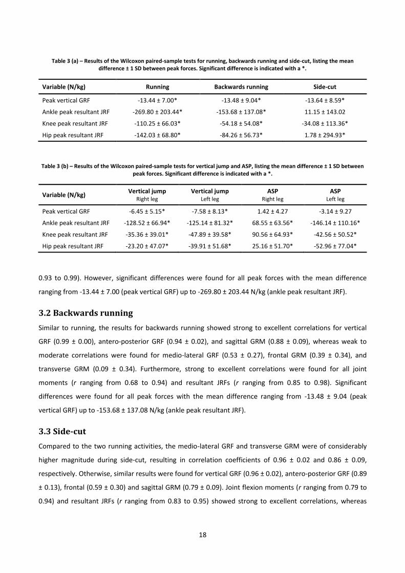
Table 3 (a) – Results of the Wilcoxon paired-sample tests for running, backwards running and side-cut, listing the mean difference ± 1 SD between peak forces. Significant difference is indicated with a *.

Variable (N/kg) Running Backwards running Side-cut

Peak vertical GRF -13.44 ± 7.00* -13.48 ± 9.04* -13.64 ± 8.59*

Ankle peak resultant JRF -269.80 ± 203.44* -153.68 ± 137.08* 11.15 ± 143.02

Knee peak resultant JRF -110.25 ± 66.03* -54.18 ± 54.08* -34.08 ± 113.36*

Hip peak resultant JRF -142.03 ± 68.80* -84.26 ± 56.73* 1.78 ± 294.93*

Table 3 (b) – Results of the Wilcoxon paired-sample tests for vertical jump and ASP, listing the mean difference ± 1 SD between peak forces. Significant difference is indicated with a *.

Variable (N/kg) Vertical jump

Right leg Vertical jump

Left leg ASP

Right leg ASP

Left leg

Peak vertical GRF -6.45 ± 5.15* -7.58 ± 8.13* 1.42 ± 4.27 -3.14 ± 9.27

Ankle peak resultant JRF -128.52 ± 66.94* -125.14 ± 81.32* 68.55 ± 63.56* -146.14 ± 110.16*

Knee peak resultant JRF -35.36 ± 39.01* -47.89 ± 39.58* 90.56 ± 64.93* -42.56 ± 50.52*

Hip peak resultant JRF -23.20 ± 47.07* -39.91 ± 51.68* 25.16 ± 51.70* -52.96 ± 77.04*

0.93 to 0.99). However, significant differences were found for all peak forces with the mean difference

ranging from -13.44 ± 7.00 (peak vertical GRF) up to -269.80 ± 203.44 N/kg (ankle peak resultant JRF).

3.2 Backwards running

Similar to running, the results for backwards running showed strong to excellent correlations for vertical

GRF (0.99 ± 0.00), antero-posterior GRF (0.94 ± 0.02), and sagittal GRM (0.88 ± 0.09), whereas weak to

moderate correlations were found for medio-lateral GRF (0.53 ± 0.27), frontal GRM (0.39 ± 0.34), and

transverse GRM (0.09 ± 0.34). Furthermore, strong to excellent correlations were found for all joint

moments (r ranging from 0.68 to 0.94) and resultant JRFs (r ranging from 0.85 to 0.98). Significant

differences were found for all peak forces with the mean difference ranging from -13.48 ± 9.04 (peak

vertical GRF) up to -153.68 ± 137.08 N/kg (ankle peak resultant JRF).

3.3 Side-cut

Compared to the two running activities, the medio-lateral GRF and transverse GRM were of considerably

higher magnitude during side-cut, resulting in correlation coefficients of 0.96 ± 0.02 and 0.86 ± 0.09,

respectively. Otherwise, similar results were found for vertical GRF (0.96 ± 0.02), antero-posterior GRF (0.89

± 0.13), frontal (0.59 ± 0.30) and sagittal GRM (0.79 ± 0.09). Joint flexion moments (r ranging from 0.79 to

0.94) and resultant JRFs (r ranging from 0.83 to 0.95) showed strong to excellent correlations, whereas

19

HAM (0.35 ± 0.36) and HERM (0.60 ± 0.22) showed a weak and moderate correlation, respectively.

Significant differences were found for all peak forces, except ankle peak resultant JRF (mean diff. = 11.15 ±

143.02 N/kg).

3.4 Vertical jump

For vertical jump, the majority of the variables showed comparable results between datasets, and similar

results for the RL and LL, highlighted by the strong to excellent correlations found for vertical GRF (0.98 ±

0.01), frontal GRM (0.96 ± 0.02), sagittal GRM (RL: 0.92 ± 0.08, LL: 0.87 ± 0.12), joint flexion moments (r

ranging from 0.95 to 0.98, median 0.96) and resultant JRFs (r ranging from 0.97 to 0.99, median 0.99).

Weak to strong correlations were found for the remaining variables (r ranging from -0.13 to 0.78, median

0.59), for which, however, the forces and moments were of considerably lower magnitude. Significant

differences were found for all peak forces with the mean difference ranging from -6.45 ± 5.15 (RL peak

vertical GRF) to 128.52 ± 66.94 N/kg (RL ankle peak resultant JRF).

3.5 ASP

Compared to vertical jump, ASP involved different movement patterns for each leg, leading to different

characteristics in the resulting kinetic data. However, the statistical results were similar between legs for

the majority of the variables with the main findings being the excellent correlations for vertical GRF (0.99 ±

0.01) and antero-posterior GRF (RL: 0.97 ± 0.02, LL: 0.99 ± 0.01), and the strong to excellent correlations

found for all joint moments (r ranging from 0.77 to 0.98, median 0.92) and resultant JRFs (r ranging from

0.78 to 0.99, median 0.94). The most notable differences between the variables associated with each leg

were the frontal (RL: 0.83 ± 0.12, LL: 0.47 ± 0.37) and sagittal GRM (RL: 0.69 ± 0.13, LL: 0.95 ± 0.03).

Significant differences were found for all peak forces, except peak vertical GRF for both the RL (mean diff. =

1.42 ± 4.27 N/kg) and LL (mean diff. = -3.14 ± 9.27 N/kg).

4. Discussion

In this study, the method of Fluit et al. (2014a) was adopted and validated for an array of movements

associated with sports, using kinematic data and a scaled musculoskeletal model only to predict GRF&Ms.

Alterations were made in an attempt to improve the original method, which included the implementation

of a new smoothing function and additional contact points to the dynamic contact model. The predicted

GRF&Ms and associated joint kinetics were compared to the corresponding variables from a model

applying a traditional IDA approach in the AMS, in which the GRF&Ms were measured using force plates.

20

Across all movements, the majority of the variables showed comparable results between datasets.

The main findings were that the model was able to provide estimates comparable to the traditional IDA

approach for vertical GRF, joint flexion moments and resultant JRFs. These results were, furthermore,

overall similar between movements involving only single support (e.g. running), entirely double support

(vertical jump) and a transition from double to single support (ASP). As described by Fluit et al. (2014a),

increased errors in the model estimates can be expected when the external forces and moments need to

be distributed over both feet. In the present study, however, the results for vertical jump surprisingly

showed the highest overall correlations for joint flexion moments and resultant JRFs. The results for the

GRMs, antero-posterior and medio-lateral GRFs varied between movements and discrepancies were

identified, particularly for the transverse and frontal GRMs. However, the discrepancies were generally

associated with variables of low magnitude and could be contributed to the influence of noise on the

correlations. The transverse GRMs showed the lowest correlations between datasets, which was consistent

with the findings of Fluit et al. (2014a). This result could be partly caused by the constraint imposed by the

simplified model of the knee as a hinge-joint, which did not allow for transversal rotation. This issue could,

furthermore, have caused the relatively poor agreement of the HERM for the majority of the movements.

Finally, despite the overall similarities in the datasets, the computed peak vertical GRFs and resultant JRFs

showed discrepancies and significant differences were established for the majority of these variables.

Previous studies in this area have applied their methods for predicting GRF&Ms to the analysis of gait

(Fluit et al., 2014a; Eel Oh et al., 2013; Ren et al., 2008), simple static postures, such as stance (Choi et al.,

2013; Audu et al., 2007), or activities of daily living, such as deep squatting and stair ascent (Fluit et al.,

2014a). This paper presented, for the first time, the prediction of GRF&Ms during movements that are

widely used in sports and recreational exercise, involving considerably higher segment accelerations and

force magnitudes compared to previous studies. It was expected that the larger accelerations in particular

could lead to inaccuracies in the kinetic measures due to the increased importance of the inertial and mass

properties of the segments. Furthermore, the higher accelerations are likely to increase errors in the

kinematic data, especially due to the larger deformations of soft tissues. However, these issues did not

appear to have a critical effect on the kinetic measures in the present study, as overall comparable results

were obtained for both the predicted GRF&Ms and the joint kinetics.

As mentioned above, the discrepancies found for the medio-lateral GRFs, frontal and transverse

GRMs could be largely contributed to the low magnitude of these variables, which increased the influence

of noise. When these variables increased in magnitude, the correlations between datasets likewise

increased, such as the frontal GRMs during vertical jump (r = 0.96 ± 0.02) and transverse GRM during side-

21

cut (r = 0.86 ± 0.09). This tendency indicates that noise was the predominant issue for these inaccuracies.

Furthermore, variables displaying such low magnitudes would presumably not be of primary interest for

most studies and the lower accuracy of these estimates could, therefore, be of minor importance.

A number of limitations should be noted. First, it is well-known that marker trajectories are

associated with noise, especially due to soft-tissue artefacts (Cappozzo et al., 2005), and methods to

sufficiently compensate for these inaccuracies does currently not exist (Benoit et al., 2015). Second, the

foot was modelled as a single segment and the dynamic contact model could have been improved by

applying a multi-segment foot model. In particular, a model that enables bending of the toes, hereby

increasing the foot-ground contact surface during toe-off. Third, the muscle models did not incorporate

excitation-contraction dynamics, which might have altered the predicted GRF&Ms, as the activation level of

the muscle-like actuators were solved as part of the muscle recruitment. Finally, the study could benefit

from a comprehensive sensitivity analysis, thus determining the influence of multiple parameters

associated with the dynamic contact model.

In order to improve the model’s prediction of GRF&Ms, a number of parameters could be adjusted in

the dynamic contact model. First, the contact point offsets were approximated, considering the sole

thickness of the running shoes and the soft tissue under the heel, and measurements of these parameters

could possibly improve the ground contact determination. However, the points are required to overlap

with the artificial ground plane in the model environment and have to be adjusted accordingly. Second, the

number and position of the contact points could be adjusted to provide more detailed modelling of the

foot-ground contact, accounting for the underside characteristics of the foot or specific footwear used.

Third, a sensitivity analysis could have been performed on the contact parameters, 𝐹𝑚𝑎𝑥, 𝑧𝑙𝑖𝑚𝑖𝑡, and 𝑣𝑙𝑖𝑚𝑖𝑡,

as well as the threshold values for 𝑧𝑟𝑎𝑡𝑖𝑜 and 𝑣𝑟𝑎𝑡𝑖𝑜, hereby determining a set of optimal values. This could

potentially have reduced the consistent overestimations of peak forces that were identified for nearly all

movements and represented the clearest discrepancy between datasets. Therefore, a comprehensive

sensitivity analysis involving all or several of the contact parameters should be deployed to find an optimal

combination, aimed towards achieving the highest possible accuracy in the model estimates.

The presented method predominately showed comparable results to traditional IDA, providing a

number of valuable opportunities for future studies, particularly within sports science research. By

obviating the need for force plate measurements, this method facilitates the analysis of sports-related

movements that occupy a large space or can only be analysed in their entirety in outdoor environments.

Furthermore, the method excludes the potential influence of force plate targeting, which was implemented

during the side-cut manoeuvre for instance. Another potential benefit of this method is that it enables the

22

determination of GRF&Ms in situations, where force plates are difficult and expensive to instrument, such

as motion analysis during treadmill walking or running. In addition, it can be combined with motion analysis

systems that do not commonly incorporate an interface between kinematic and force plate data, for

example, electromagnetic tracking systems (Frantz et al., 2003) or a combination of miniature gyroscopes

and accelerometers (Luinge and Veltink, 2005). Finally, an exciting perspective is the combination of the

method with marker-less motion capture systems, as for instance the method presented in Sandau et al.

(2014), or incorporating the method in prospective simulations (Fluit et al. 2014b). Recently, Skals et al.

(2014) introduced an interface between marker-less motion capture data and a musculoskeletal model,

incorporating the method for predicting GRF&Ms of Fluit et al. (2014a), thus providing the first step

towards complete IDA using such systems. Therefore, future studies should continue exploring new and

improved approaches for marker-less motion analysis to obtain a sufficient level of accuracy as well as

continually improve methods for predicting GRF&Ms, particularly focusing on models for accurate ground

contact determination.

5. Conclusion

Prediction of GRF&Ms can reduce dynamic inconsistency and obviate the need for force plate

measurements when performing IDA on musculoskeletal models. This study provided validation of a

method to predict GRF&Ms from full-body motion only for an array of sports-related movements. The

method provided estimates comparable to traditional IDA for the majority of the analysed variables,

including vertical GRF, joint flexion moments and resultant JRFs. Based on these results, the method could

be used instead of force plate data when performing IDA, hereby facilitating the analysis of sports-related

movements and providing new opportunities for complete IDA using systems that does not provide and

interface between kinematic and force plate data.

6. References

Andersen, M. S., Damsgaard, M., MacWilliams, B. & Rasmussen, J. 2010, "A computationally efficient optimisation-

based method for parameter identification of kinematically determinate and over-determinate

biomechanical systems", Comput. Methods Biomech. Biomed. Engin., vol. 13, no. 2, pp. 171–183.

Andersen, M. S., Damsgaard, M. & Rasmussen, J. 2009, "Kinematic analysis of over-determinate biomechanical

systems", Comput. Methods Biomech. Biomed. Engin., vol. 12, no. 4, pp. 371–384.

Anderson, F. C. & Pandy, M. G. 2001, "Dynamic optimization of human walking", J. Biomech. Eng., vol. 123, no. 5, pp.

381-190.

23

The AnyBody Modeling System (Version 6.05) (2015). [Computer software]. Aalborg, Denmark: AnyBody Technology.

Available from http://www.anybodytech.com

Audu, M. L., Kirsch, R. F. & Triolo, R. J. 2007, "Experimental verification of a computational technique for determining

ground reactions in human bipedal stance", J. Biomech., vol. 40, no. 5, pp. 1115–1124.

Audu, M. L., Kirsch, R. F. & Triolo, R. J. 2003, "A computational technique for determining the ground reaction forces in

human bipedal stance", J. Appl. Biomech., vol. 19, no. 4, pp. 361–371.

Barret, R. S., Besier, T. F. & Lloyd, D. G. 2007, "Individual muscle contributions to the swing phase of gait: An EMG-

based forward dynamics modelling approach", Simul. Model. Pract. Th., vol. 15, no. 9, pp. 1146-1155.

Benoit, D. L., Damsgaard, M. & Andersen, M. S. 2015, "Surface marker cluster translation, rotation, scaling and

deformation: Their contribution to soft tissue artefact and impact on knee joint kinematics", J. Biomech.,

Available online 27 March 2015, http://dx.doi.org/10.1016/j.jbiomech.2015.02.050.

Cahouët, V., Luc, M. & David, A. 2002, "Static optimal estimation of joint accelerations for inverse dynamics problem

solution", J. Biomech., vol. 35, no. 11, pp. 1507–1513.

Cappozzo, A., Della Croce, U., Leardini, A. & Chiari, L. 2005, "Human movement analysis using stereophotogrammetry.

Part 1: theoretical background", Gait Posture, vol. 21, no. 2, pp. 186–196.

Carbone, V., Fluit, R., Pellikaan, P., van der Krogt, M. M., Jansen, D., Damsgaard, M., Vigneron, L., Feilkas, T., Koopman,

H. F. J. M., Verdonschot, N. 2015, "TLEM 2.0 - A comprehensive musculoskeletal geometry dataset for

subject-specific modeling of lower extremity", J. Biomech., vol. 48, no. 5, pp. 734-741.

Challis, J. H. 2001, "The variability in running gait caused by force plate targeting", J. Appl. Biomech., vol. 17, no. 1, pp.

77–83.

Chiari, L., Croce, U. D., Leardini, A. & Cappozzo, A. 2005, "Human movement analysis using stereophotogrammetry.

Part 2: Instrumental errors", Gait Posture, vol. 21, no. 2, pp. 197–211.

Choi, A., Lee, J.-M. & Mun, J. H. 2013, "Ground reaction forces predicted by using artificial neural network during

asymmetric movements", Int. J. Precis. Eng. Manuf., vol. 14, no. 3, pp. 475–483.

Clauser, C. E., McConville, J. T. & Young, J. W. 1969, "Weight, volume, and center of mass of segments of the human

body", DTIC Document.

Collins, S. H., Adamczyk, P. G., Ferris, D. P. & Kuo, A. D. 2009, "A simple method for calibrating force plates and force

treadmills using an instrumented pole", Gait Posture, vol. 29, no. 1, pp. 59-64.

Damsgaard, M., Rasmussen, J., Christensen, S. T., Surma, E. & de Zee, M. 2006, "Analysis of musculoskeletal systems in

the AnyBody Modeling System", Simul. Model. Pract. Theory, vol. 14, no. 8, pp. 1100–1111.

Della Croce, U., Leardini, A., Chiari, L. & Cappozzo, A. 2005, "Human movement analysis using stereophotogrammetry.

Part 4: assessment of anatomical landmark misplacement and its effects on joint kinematics", Gait Posture,

vol. 21, no. 2, pp. 226–237.

Delp, S. L., Anderson, F. C., Arnold, A. S., Loan, P., Habib, A., John, C. T., Guendelman, E. & Thelen, D. G. 2007,

"OpenSim: Open-Source Software to Create and Analyze Dynamic Simulations of Movement", IEEE Trans.

Biomed. Eng., vol. 54, no. 11, pp. 1940–1950.

24

Eel Oh, S., Choi, A. & Mun, J. H. 2013, "Prediction of ground reaction forces during gait based on kinematics and a

neural network model", J. Biomech., vol. 46, no. 14, pp. 2372–2380.

Erdemir, A., McLean, S. & Herzog, W. 2007, "Model-Based Estimation of Muscle Forces Exerted during Movements",

Clin. Biomech., vol. 22, no. 2, pp. 131-154.

Fluit, R., Andersen, M. S., Kolk, S., Verdonschot, N. & Koopman, H. F. J. M. 2014a, "Prediction of ground reaction forces

and moments during various activities of daily living", J. Biomech., vol. 47, no. 10, pp. 2321–2329.

Fluit, R., Andersen, M. S., Verdonschot, N., Koopman, H. F. J. M. 2014b, "Optimal inverse dynamic simulation of human

gait", Gait Posture, vol. 39, Supplement 1, pp. S42.

Frantz, D. D., Wiles, A. D., Leis, S. E. & Kirsch, S. R. 2003, "Accuracy assessment protocols for electromagnetic tracking

systems", Phys. Med. Biol., vol. 48, no. 14, pp. 2241-2251.

Hatze, H. 2002, "The fundamental problem of myoskeletal inverse dynamics and its implications", J. Biomech., vol. 35,

no. 1, pp. 109–115.

Horsman, M. D. K., Koopman, H. F. J. M., van der Helm, F. C. T., Prosé, L. P., Veeger, H. E. J. 2007, "Morphological

muscle and joint parameters for musculoskeletal modelling of the lower extremity", Clin. Biomech., vol. 22,

no. 2, pp. 239–247.

Kuo, A. D. 1998, "A least-squares estimation approach to improving the precision of inverse dynamics computations",

J. Biomech. Eng., vol. 120, no. 1, pp. 148-159.

Leardini, A., Chiari, L., Croce, U. D. & Cappozzo, A. 2005, "Human movement analysis using stereophotogrammetry.

Part 3. Soft tissue artifact assessment and compensation", Gait Posture, vol. 21, no. 2, pp. 212–225.

Luinge, H. J. & Veltink, P. H. 2005, "Measuring orientation of human body segments using miniature gyroscopes and

accelerometers", Med. Biol. Eng. Comput., vol. 43, no. 2, pp. 273–282.

Lund, M. E., Andersen, M. S., de Zee, M. & Rasmussen, J. 2015, "Scaling of musculoskeletal models from static and

dynamic trials", Int. Biomech., vol. 2, no. 1, pp. 1–11.

Mellon, S. J., Grammatopoulos, G., Andersen, M. S., Pegg, E. C., Pandit, H. G., Murray, D. W. & Gill, H. S. 2013,

"Individual motion patterns during gait and sit-to-stand contribute to edge-loading risk in metal-on-metal hip

resurfacing", Proc. Inst. Mech. Eng. H J. Eng. Med., vol. 227, no. 7, pp. 799-810.

Mellon, S. J., Grammatopoulos, G., Andersen, M. S., Pandit, H. G., Gill, H. S. & Murray, D. W. 2015, "Optimal acetabular

component orientation estimated using edge-loading and impingement risk in patients with metal-on-metal

hip resurfacing arthroplasty", J. Biomech, vol. 48, no. 2, pp. 318-323.

Middleton, J., Sinclair, P. & Patton, R. 1999, "Accuracy of centre of pressure measurement using a piezoelectric force

platform", Clin. Biomech., vol. 14, no. 14, pp. 357–360.

Nigg, B. M. 2006. Force. In: NIGG, B. M. & HERZOG, W. (ed.) Biomechanics of the Musculo-skeletal System, Third

Edition. Chichester, England: John Wiley & Sons Ltd.

Pàmies-Vilà, R., Font-Llagunes, J. M., Cuadrado, J. & Alonso, F. J. 2012, "Analysis of different uncertainties in the

inverse dynamic analysis of human gait", Mech. Mach. Theory, vol. 58, pp. 153–164.

Payton, C. J. & Bartlett, R. M. 2008, Biomechanical evaluation of movement in sport and exercise, Abingdon, United

Kingdom: Routledge.

25

Pearsall, D. J. & Costigan, P. A. 1999, "The effect of segment parameter error on gait analysis results", Gait Posture,

vol. 9, no. 3, pp. 173–183.

Psycharakis, S. G. & Miller, S. 2006, "Estimation of Errors in Force Platform Data", Res. Q. Exerc. Sport, vol. 77, no. 4,

pp. 514–518.

Rao, G., Amarantini, D., Berton, E. & Favier, D. 2006, "Influence of body segments’ parameters estimation models on

inverse dynamics solutions during gait", J. Biomech., vol. 39, no. 8, pp. 1531–1536.

Rasmussen, J., Dahlquist, J., Damsgaard, M., de Zee, M. & Christensen, S. T. 2003a, "Musculoskeletal modeling as an

ergonomic design method", in: Proceedings of the XVth Triennial Congress of the International Ergonomics

Association and 7th Joint Conference of the Ergonomics Society of Korea/Japan Ergonomics Society, Seoul,

Korea.

Rasmussen, J., Damsgaard, M., Surma, E., Christensen, S. T., de Zee, M. & Vondrak, V. 2003b, "Anybody - a software

system for ergonomic optimization", in: Fifth World Congress on Structural and Multidisciplinary

Optimization, Venice, Italy.

Rasmussen, J., Damsgaard, M. & Voigt, M. 2001, "Muscle recruitment by the min/max criterion—a comparative

numerical study", J. Biomech., vol. 34, no. 3, pp. 409–415.

Ren, L., Jones, R. K. & Howard, D. 2008, "Whole body inverse dynamics over a complete gait cycle based only on

measured kinematics", J. Biomech., vol. 41, no. 12, pp. 2750–2759.

Riemer, R. & Hsiao-Wecksler, E. T. 2008, "Improving joint torque calculations: Optimization-based inverse dynamics to

reduce the effect of motion errors", J. Biomech., vol. 41, no. 7, pp. 1503–1509.

Riemer, R., Hsiao-Wecksler, E. T. & Zhang, X. 2008, "Uncertainties in inverse dynamics solutions: A comprehensive

analysis and an application to gait", Gait Posture, vol. 27, no. 4, pp. 578–588.

Robert, T., Causse, J. & Monnier, G. 2013, "Estimation of external contact loads using an inverse dynamics and

optimization approach: General method and application to sit-to-stand maneuvers", J. Biomech., vol. 46, no.

13, pp. 2220-2227.

Sandau, M., Koblauch, H., Moeslund, T. B., Aanæs, H., Alkjær, T. & Simonsen, E. B. 2014, "Markerless motion capture

can provide reliable 3D gait kinematics in the sagittal and frontal plane", Med. Eng. Phys., vol. 36, no. 9, pp.

1168-1175.

Schwartz, M. H. & Rozumalski, A. 2005, "A new method for estimating joint parameters from motion data", J.

Biomech., vol. 38, no. 1, pp. 107-116.

Skals, S. L., Bendtsen, K. M., Rasmussen, K. P. & Andersen, M. S. 2014, "Validation of musculoskeletal models driven by

dual Microsoft Kinect Sensor data", in: 13th

International Symposium on 3D Analysis of Human Movement,

Lausanne, Switzerland.

Stagni, R., Fantozzi, S., Cappello, A. & Leardini, A. 2005, "Quantification of soft tissue artefact in motion analysis by

combining 3D fluoroscopy and stereophotogrammetry: a study on two subjects", Clin. Biomech., vol. 20, no.

3, pp. 320–329.

Taylor, R. 1990, "Interpretation of the correlation coefficient: a basic review", J. Diagn. Med. Sonog., vol. 6, no. 1, pp.

35-39.

26

Thelen, D. G. & Anderson, F. C. 2006, "Using computed muscle control to generate forward dynamic simulations of

human walking from experimental data", J. Biomech., vol. 39, no. 6, pp. 1107-1115.

Van der Helm, F. C. T., Veeger, H. E. J., Pronk, G. M., Van der Woude, L. H. V. & Rozendal, R. H. 1992, "Geometry

parameters for musculoskeletal modelling of the shoulder system", J. Biomech., vol. 25, no. 2, pp. 129-144.

Vaughan, C. L., Davis, B. L. & O'Connor, J. C. 1999, Dynamics of Human Gait, Second Edition, Western Cape, South

Africa: Kiboho Publishers.

Vaughan, C. L., Andrews, J. G. & Hay, J. G. 1982, "Selection of body segment parameters by optimization methods", J.

Biomech. Eng., vol. 104, no. 1, pp. 38-44.

Veeger, H. E. J., Van der Helm, F. C. T., Van der Woude, L. H. V., Pronk, G. M. & Rozendal, R. H. 1991, "Inertia and

muscle contraction parameters for musculoskeletal modelling of the shoulder mechanism", J. Biomech., vol.

24, no. 7, pp. 615-629.

Weber, T., Al-Munajjed, A. A., Verkerke, G. J., Dendorfer, S. & Renkawitz, T. 2014, "Influence of minimally invasive

total hip replacement on hip reaction forces and their orientations", J. Orthop. Res., vol. 32, no. 12, pp. 1680-

1687.

Zajac, F. E., Neptune, R. R. & Kautz, S. A. 2003, "Biomechanics and muscle coordination of human walking: part II:

lessons from dynamical simulations and clinical implications", Gait Posture, vol. 17, no. 1, pp. 1–17.

de Zee, M., Hansen, L., Wong, C., Rasmussen, J. & Simonsen, E. B. 2007, "A generic detailed rigid-body lumbar spine

model", J. Biomech., vol. 40, no. 6, pp. 1219-1227.

Appendix

Label Position A-P M-L P-D

RTHI

Right thigh Opt. Opt. Opt.

LTHI

Left thigh Opt. Opt. Opt.

RKNE Right lateral epicondyle Fix. Fix. Fix.

LKNE Left lateral epicondyle Fix. Fix. Fix.

RPSI

Right posterior superior iliac spine Fix. Fix. Fix.

LPSI

Left posterior superior iliac spine Fix. Fix. Fix.

RASI Right anterior superior iliac spine Fix. Fix. Fix.

LASI Left anterior superior iliac spine Fix. Fix. Fix.

RANK Right lateral malleolus Fix. Fix. Fix.

LANK Left lateral malleolus Fix. Fix. Fix.

RHEE Right calcaneus Fix. Fix. Fix.

LHEE Left calcaneus Fix. Fix. Fix.

RTIB

Right tibia Opt. Opt. Opt.

LTIB

Left tibia Opt. Opt. Opt.

RTOE Right metatarsus Fix. Fix. Fix.

LTOE Left metatarsus Fix. Fix. Fix.

RMT5 Right fifth metatarsal Fix. Fix. Fix.

LMT5 Left fifth metatarsal Fix. Fix. Fix.

RELB Right lateral epicondyle Fix. Fix. Fix.

LELB Left lateral epicondyle Fix. Fix. Fix.

RWRA Right wrist bar thumb side Fix. Fix. Fix.

LWRA Left wrist bar thumb side Fix. Fix. Fix.

RFINL Right first metacarpal Fix. Fix. Fix.

LFINL Left first metacarpal Fix. Fix. Fix.

RFINM Right fifth metacarpal Fix. Fix. Fix.

LFINM Left fifth metacarpal Fix. Fix. Fix.

RUPA

Right triceps brachii Opt. Opt. Opt.

LUPA

Left triceps brachii Opt. Opt. Opt.

RSHO Right Acromio-clavicular joint Fix. Fix. Fix.

LSHO Left Acromio-clavicular joint Fix. Fix. Fix.

STRN

Xiphoid process of the sternum Opt. Opt. Opt.

CLAV

Jugular Notch Opt. Opt. Fix.

C7 7th Cervical Vertebrae Fix. Fix. Fix.

RILC* Right iliac crest - - -

LILC* Left iliac crest - - -

*Excluded

Appendix 1 – Marker protocol, listing marker labels, positions and whether the marker positions were fixed (Fix.) or optimized

(Opt.) in the antero-posterior (A-P), medio-lateral (M-L) and proximal-distal (P-D) directions.

AALBORG UNIVERSITY

Prediction of ground reaction forces and moments during sports-related movements

Worksheets

Sebastian Laigaard Skals

2/6/2015

Contents Worksheet 1 - Theoretical Background ............................................................................................................................. 1

1. Musculoskeletal modelling .................................................................................................................................. 1

1.1 Objectives and challenges ...................................................................................................................... 2

1.2 Model structure ..................................................................................................................................... 3

1.3 Body segment parameters ..................................................................................................................... 4

1.4 Analytical approaches ............................................................................................................................ 6

2. Inverse dynamics in the AnyBody Modeling System ........................................................................................... 7

2.1 Kinematics .............................................................................................................................................. 7

2.1.1 Marker-based motion analysis......................................................................................................... 8

2.1.2 Kinematic analysis in the AnyBody Modeling System ...................................................................... 9

2.2 Kinetics ................................................................................................................................................. 12

2.2.1 Muscle recruitment ....................................................................................................................... 13

2.2.2 External forces ............................................................................................................................... 14

2.2.3 Solving the equations of motion .................................................................................................... 16

3. Errors associated with experimental input data ............................................................................................... 17

3.1 Estimating body segment parameters ................................................................................................. 18

3.2 Marker-based motion analysis: Measurement errors and reliability ................................................... 18

3.3 Force plates: Instrumental errors and calibration ................................................................................ 19

3.4 Over-determinacy and dynamic inconsistency .................................................................................... 20

4. Prediction of ground reaction forces ................................................................................................................. 21

5. References ......................................................................................................................................................... 22

Worksheet 2 - Information for participants and consent form ........................................................................................ 1

Time and location .................................................................................................................................................... 1

Introduction ............................................................................................................................................................. 2

Experimental procedure .......................................................................................................................................... 2

Participant inclusion and exclusion criteria ............................................................................................................. 3

Risks or disadvantages ............................................................................................................................................. 4

Anonymity ............................................................................................................................................................... 4

Accessibility and publication ................................................................................................................................... 4

Benefits associated with participation .................................................................................................................... 4

Participant rights ..................................................................................................................................................... 4

Practical information ............................................................................................................................................... 4

Consent form ........................................................................................................................................................... 5

1

Theoretical Background

Musculoskeletal modelling has become an inherent part of many areas of research providing insight into

the internal forces acting in the body during motion, which are otherwise impractical or impossible to

measure. This is accomplished by viewing the human body as a mechanical system consisting of rigid

bodies, which enables analysis of the system’s behaviour using methods associated with multibody

dynamics. Nowadays, several commercial software packages exist that enables detailed and fairly efficient

simulation of the musculoskeletal system. This does not mean, however, that computer simulation of the

musculoskeletal system is independent from experimental data. On the contrary, these models rely on

many different experimental inputs and the quality of these data strongly affects the accuracy of the

models’ estimation of internal forces. One of these inputs is the external forces acting on the body by the

environment, which are measured using various sensors depending on e.g. the task and environment

included in the simulation. For studies of human motion, the most commonly measured external forces are

the ground reaction forces and moments (GRF&Ms), which are typically obtained using force plates (FP).

However, as will become clear in the following, this input can contribute to errors in the model outputs

while the dependency on FP measurements imposes practical limitations during motion analysis studies.

In the following, the fundamental information about the procedures associated with the present

study is presented by providing an overview of the mechanical analysis of the musculoskeletal system,

specifically Inverse Dynamic Analysis (IDA). First, the area of musculoskeletal modelling is described,

including applications, principles and assumptions, and the overall structure of models. Second, IDA is

described in more detail, focusing on the specific approach inherent to the AnyBody Modeling System

(AMS) (AnyBody Technology A/S, Aalborg, Denmark) as well as the various experimental inputs to the

analysis and associated errors. Finally, limitations of the current approach for IDA are described, focusing

on the potential benefits of predicting rather than measuring GRF&Ms.

1. Musculoskeletal modelling

For many years, computer models have been applied to nearly all areas of engineering and are now an

indispensable tool to the extent that computer-aided methods have replaced physical experiments for

many prototype designs (Lund et al., 2012). The primary benefit associated with creating simulations of the

musculoskeletal system is that these models provide estimates of the body’s internal behaviour, which are

otherwise difficult or impossible to measure experimentally (Zajac and Winthers, 1990). As described by

2

Pandy (2001), there is a growing belief that musculoskeletal models are able to provide quantitative

explanations of how the neuromuscular and musculoskeletal systems interact to produce movement. This

belief partly stems from the continuing development of computer systems, which, along with advances in

numerical procedures, enables the development and analysis of more comprehensive and, therefore, more

realistic models of the musculoskeletal system (Huston, 2001; Pandy, 2001). Today, the application of

musculoskeletal models has become more widespread within science and industry due to the availability of

modelling software, such as SIMM (Delp and Loan, 1995), OpenSIM (Delp et al., 2007) and the AMS.

Musculoskeletal models are now being applied in ergonomic optimization of products and workplaces

(Rasmussen et al., 2003a, 2003b), treatment of gait abnormalities (Arnold and Delp, 2005; Zajac et al.,

2003), orthopaedics (Mellon et al., 2013, 2015; Weber et al., 2014) and sports biomechanics (Payton and

Bartlett, 2008) (Figure 1). Considering these developments, computer simulation could potentially achieve

the same significance for studies of the musculoskeletal system as it has for other areas of engineering.

1.1 Objectives and challenges

In general, computer simulation models can be used to 1) increase knowledge and insight about a complex

situation and/or 2) estimate how important variables are sensitive to changes in internal or external

conditions (Nigg et al., 2006). The mechanical function of the human body is indeed a complex situation. As

described by Nigg et al. (2006), the muscles are the active components producing force while bone,

cartilage, ligaments and tendons provide various passive functions. The skeletal system can move at joints

and the mechanical properties of the joints determine the translational and rotational movement

possibilities between body segments. The muscles are activated by the central nervous system (CNS), which

chooses a set of muscle actions that enables a desired motion for any position, movement or loading

condition (Rasmussen et al., 2001).

From a mechanical point of view, the complexity of the human body partly stems from the geometric

and material properties of the system (Huston, 2001). The skeletal structure, muscles and other soft tissues

constitute a highly complex geometry and the material properties of the body are irregular, which

complicates or prevents the determination of their mechanical function. In addition, two of the main

challenges when attempting to describe the dynamics of human motion are the mechanical properties of

muscles and the muscle activation pattern. As described by Herzog (2006), many aspects of muscular force

production have still not been resolved mainly due to their complicated contractile properties. Likewise,

the activation of muscles by the CNS to produce complex movement remains poorly understood

(Damsgaard et al., 2006; Manal and Buchanan, 2004). Therefore, computer models need to be simplified

and general assumptions about the system’s mechanical function are necessary to enable analysis.

3

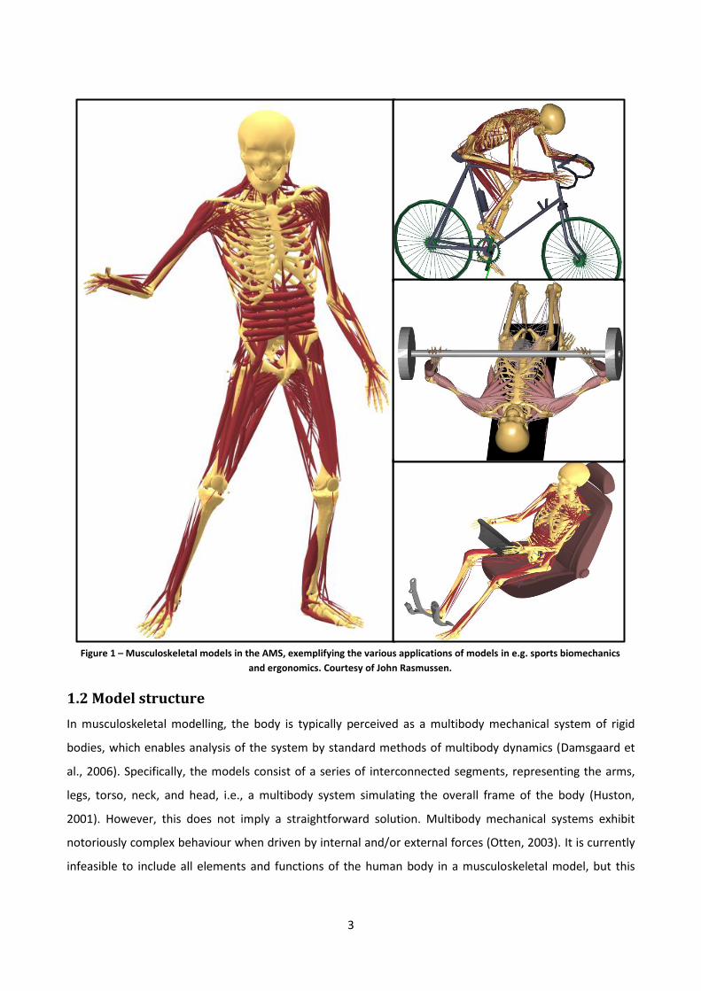
1.2 Model structure

In musculoskeletal modelling, the body is typically perceived as a multibody mechanical system of rigid

bodies, which enables analysis of the system by standard methods of multibody dynamics (Damsgaard et

al., 2006). Specifically, the models consist of a series of interconnected segments, representing the arms,

legs, torso, neck, and head, i.e., a multibody system simulating the overall frame of the body (Huston,

2001). However, this does not imply a straightforward solution. Multibody mechanical systems exhibit

notoriously complex behaviour when driven by internal and/or external forces (Otten, 2003). It is currently

infeasible to include all elements and functions of the human body in a musculoskeletal model, but this

Figure 1 – Musculoskeletal models in the AMS, exemplifying the various applications of models in e.g. sports biomechanics

and ergonomics. Courtesy of John Rasmussen.

4

does not mean that models cannot provide accurate estimations of the body’s mechanical function and,

hereby, improve our understanding of the underlying mechanisms of human locomotion.

In general, which elements to include in a musculoskeletal model depends on its intended use and it

is generally accepted that the simplest model fulfilling the goal of the research should be deployed (Pandy,

2001; Zajac and Winthers, 1990). This is partly due to the fact that despite the advances in computational

resources, musculoskeletal models still need to be highly simplified in order to be reasonably efficient

(Damsgaard et al., 2006). As described by Pandy (2001), if the goal of the model is to describe muscle

function, the structures contributing to the overall stiffness of the joint are rarely included, such as

cartilage, menisci and ligaments. For other applications, however, the contribution of these passive

structures might be crucial to obtain accurate simulation results. In a recent example of detailed knee

modelling, ligaments were represented as spring elements with nonlinear elastic characteristics (Marra et

al., 2015). According to Zajac and Winthers (1990), there are seven major steps that need to be included in

a musculoskeletal model to account for multi-muscle control of the body segments during motion. 1) The

body segments and joint kinematics must be specified. 2) The dynamical equations of motion must be

derived, which depends on the assumed properties of the joints and interaction between the body

segments and the environment. 3) Passive-joint tissue mechanics should be modelled unless assumed

insignificant, which is often the case as mentioned above. 4) Geometric joint transformation, where the

joint and musculoskeletal geometry is defined, i.e., the musculoskeletal moment arms relative to the joints’

axes of rotations. 5) The musculotendon force generation process, which involves the musculotendon

structural properties and the dynamical properties of the musculotendon actuator (e.g. muscle excitation-

contraction coupling and musculotendon contraction dynamics). 6) The neuromotor CNS circuitry, also

known as muscle recruitment pattern, which describes how individual muscles are recruited/activated

during coordinated movement. 7) The complete musculoskeletal model is specified by the interaction

between these constituent parts.

1.3 Body segment parameters

Although quite simple models can be adequate for many purposes, it is obvious that more comprehensive

and detailed models possess greater potential for providing accurate simulations of the human body.

Estimating body segment parameters (BSPs) involves defining the dynamical properties of each body

segment by personalising the model to the individual or group it aims to represent (Vaughan et al., 1999).

Typically, this can be achieved by measuring total body mass and segment lengths of a subject and applying

regression equations to define each segment’s mass, centre-of-gravity (COG) and moment-of-inertia (MOI)

(Contini et al., 1963). These regression equations are most often derived from cadaver-based studies, which

5

determine the ratio between e.g. total body mass and segment masses (Clauser et al., 1969). While this

information can be used to estimate net torques and forces at the joints, the muscular geometry and other

properties, such as muscle insertion points and wrapping surfaces, needs to be reasonably defined if one

wishes to determine the force exerted by individual muscles. The geometric definition of the

musculoskeletal system will define the moment arms as well as the length of the associated muscles,

which, taken together, determines the possible moment that can be produced at the joints by a given

muscle force (Horsman et al., 2007). In order to meet these objectives, BSPs are most often determined

generally and, subsequently, scaled to the individual or population group the model aims to represent.

The fundamental approach for determining BSPs is cadaver-based studies, such as Clauser et al.

(1969) and Carbone et al. (2015). In summary, this procedure involves dissecting a human cadaver and

performing various measurements to determine the dimensions, mass, COG and MOI of the severed body

segments. Subsequently, regression equations can be formulated based on these descriptive data, which

provides estimates of the BSPs in relation to the characteristics of the individual or group of interest. In

recent years, these descriptive data have become more detailed. Carbone et al. (2015) and Horsman et al.

(2007) used a cadaver-based study to determine additional parameters, as for instance attachment sites of

muscles, optimal muscle fibre length and pennation angles. Commonly, the cadaver-based data, providing a

more general description of the BSPs and muscular geometry, are combined with subject specific data in

order to personalise the model, also referred to as model scaling (Lund et al., 2015). For example, Vaughan

et al. (1999) determined BSPs by performing multiple anthropometric measurements to determine the

segment dimensions of their subjects and combined this information with regression coefficients obtained

through cadaver-based studies. This exemplifies model scaling based on traditional anthropometric

measurements, but, in more recent years, scaling has been performed using kinematic data (Lund et al.,

2015; Andersen et al., 2010). This approach involves scaling the model based on the position of markers

placed at bony landmarks, hence providing an estimate on the skeletal dimensions. Another approach is to

perform various scans, such as full body X-ray absorptiometry (Ganley and Powers, 2004), which provides

personalised BSP estimates on living subjects. In addition, medical imaging data from living subjects can be

used to perform detailed subject-specific scaling. Recently, Carbone et al. (2015) presented the Twente

Lower Extremity Model 2.0, which is a cadaver-based musculoskeletal model of the lower extremities

accompanied by a coherent set of medical imaging data (CT and MRI). The model is freely available and was

developed to be easily combined with other imaging data, facilitating detailed subject-specific scaling.

Although scanning techniques are considered very accurate, it typically entails high cost and radiation

exposure and should be questioned as a routine method (Vaughan et al., 1999).

6

In the AMS, anthropometric (e.g. Peebles and Norris (1998)) and/or cadaver-based data (e.g.

Horsman et al. (2007)) have been used to construct the musculoskeletal models and there are several

scaling options, closely corresponding to the different approaches described above. The standard models,

based on anthropometric measurements, can be specified to a specific percentile, i.e., the dimensions of

the population group of interest. These models can, furthermore, be scaled according to joint-to-joint

distances (resembling subject-specific anthropometric measurements), location of bony landmarks

(kinematic measurements) and/or subject-specific imaging scans. Another important aspect of scaling is the

model’s assumed muscle strength. In the AMS, muscle strength is scaled according to the height and mass

of the subjects, meaning that a taller and heavier individual will require a lower percentage of total muscle

activity to balance a given load compared to a shorter and lighter individual. Additionally, a scaling law can

be applied that takes the individual’s fat percentage into account. A higher estimated fat percentage will

result in less muscle strength, as the volume occupied by muscles is replaced by inactive fat.

1.4 Analytical approaches

While section 1.2 and 1.3 outline the general model structure and personalisation, respectively, there are a

number of different analytical approaches to study the biomechanics of human motion. Overall, these

approaches are driven by the equations of motion, which provides the relationship between motion and

forces in the mechanical system. The equations of motion can be solved in two directions, i.e., by 1) solving

the motion from the forces or 2) solving the forces from the motion (Otten, 2003). The approaches mainly

associated with 1 include Forward Dynamics-based tracking methods (Thelen and Anderson, 2006), EMG-

driven forward dynamics (Barret et al., 2007), and Dynamic Optimization (Anderson and Pandy, 2001).

Forward Dynamics-based tracking methods use computed muscle control, employing a feedforward and

feedback control, which is held up against measured kinematics to determine the muscle actions that

produce the motion (Thelen and Anderson, 2006). EMG-driven forward dynamics involves either identifying

the timing of muscle activations from EMG-data to generate a simplified neural input signal (indirect

approach) or using the continuous varying time history of the EMG-signal as the neural input to each

muscle in the model (direct approach) (Barret et al., 2007). Dynamic Optimization predicts the motor

patterns and kinematics of a given motion by solving an optimization problem for the complete movement

cycle, implementing a time-dependent performance criterion, i.e., the goal of the motor task (Anderson

and Pandy, 2001). The approach mainly associated with 2 is called Inverse Dynamics (Erdemir et al., 2007;

Damsgaard et al., 2006). IDA applies measurements of body motion and/or external forces as input to the

equations of motion to calculate muscle- and joint forces, solving a different optimization problem for each

instant during the motion (Pandy, 2001). This inherent feature improves its computational efficiency, which

can be exploited to build more complex models, i.e., a finer level of detail and a higher number of muscles

7

(Damsgaard et al., 2006; Rasmussen et al., 2001). In the present study, the musculoskeletal models are

constructed and analysed in the AMS, which exclusively allows for IDA (Damsgaard et al., 2006). Therefore,

the specific IDA approach inherent to the AMS will be described in more detail in the following.

2. Inverse dynamics in the AnyBody Modeling System

In general, IDA applies the following input to solve the dynamics of a given motion (Vaughan et al., 1999):

1) BSPs, as described in section 1.3, 2) segment kinematics, i.e., linear- and angular kinematics of body

segments, and 3) the external forces acting on the body. If only the BSPs and kinematics are known, the IDA

can be completed by iteratively solving the equations of motion for each body segment, using the so-called

top-down approach (Riemer and Hsiao-Wecksler, 2008; Cahouët et al., 2002). However, this approach is

particularly sensitive to uncertainties in the kinematic data, which can lead to inaccurate joint moment

estimations (Cahouët et al., 2002). Alternatively, the bottom-up approach can be used, which includes

measurements of the external forces acting on the bottom-most segment, typically the GRF&Ms (Riemer

and Hsiao-Wecksler, 2008; Kuo, 1998; Zajac, 1993). When the GRF&Ms are known, they form a boundary

condition for the bottom-most segment and dynamic equilibrium is obtained at each successive segment

proceeding upwards (Kuo, 1998). By inputting these external forces and moments, the inaccuracies caused

by the acceleration inputs can be reduced and the joint moment estimations tends to be more accurate in

the bottom part of the multibody system (Riemer and Hsiao-Wecksler, 2008; Zajac, 1993). The improved

accuracy of the bottom-up approach is partly due to the fact that external force data is typically less noisy

than acceleration data (Kuo, 1998). In the AMS, however, the dynamics of a given motion are not solved

iteratively by obtaining equilibrium one segment at a time throughout the kinetic chain. Instead, the muscle

and joint forces are calculated by formulating one complete set of dynamic equilibrium equations, whether

external forces are included or not (Damsgaard et al., 2006). Solving the dynamic equilibrium equations are,

however, preceded by the kinematic analysis, which provides the linear and rotational acceleration of each

segment in the model and, together with the boundary conditions, is used to form the equations of motion

(Andersen et al., 2009).

2.1 Kinematics

There are multiple methods for performing kinematic analysis that vary greatly in complexity, cost, and

accuracy, and the choice of method is typically based on a compromise between these factors. Currently,

golden standards for motion analysis include bone-pin studies (Benoit et al., 2006) and 3D fluoroscopy

(Stagni et al., 2005), which have very high accuracy. However, bone-pin studies are invasive and 3D

fluoroscopy exposes the subject to some degree of radiation while the fluoroscopic field-of-view limits the

8

analysis to small areas of the body. Another approach is to use wearable inertial motion sensors, such as

electromagnetic tracking systems (Frantz et al., 2003) or a combination of miniature gyroscopes and

accelerometers (Luinge and Veltink, 2005), which are, however, sensitive to magnetic disturbance and

require relatively large data processing units to be fixated on the body, respectively (Fong and Chan, 2010).

The most common method for motion analysis is marker-based motion capture, which applies an infrared

camera-based system to track the trajectories of reflective skin-markers placed on the body (Figure 2)

(Andersen et al., 2009; McGinley et al., 2009; Cappozzo et al., 2005; Manal and Buchanan, 2004; Richards,

1999).

2.1.1 Marker-based motion analysis

There are two camera-based systems for studying human movement, applying either active or passive

markers (Manal and Buchanan, 2004). In the present study, a passive-marker system was applied, which is

briefly explained in the following based on the descriptions by Manal and Buchanan (2004) and Chiari et al.

(2005). Passive markers, or tracking targets, basically reflect projected light, which makes the markers

visible to the camera system. In order to reflect more light than surrounding objects, markers are covered

in a highly reflective material. A ring of stroboscopic LED’s are built into the camera-system to illuminate

the markers, enabling each camera to detect markers in their line-of-sight. Subsequently, the 3-D

coordinates of each marker can be determined from the multiple 2-D camera views, which are

synchronised during an initial calibration procedure. When a marker is visible by multiple cameras, the

unique 3-D position of the marker in object-space can be determined as the intersection of rays directed

from each camera.

There are multiple approaches for positioning the markers on the body. For gait analysis, for

example, many different data acquisition protocols exist, employing different marker-sets and collection

procedures as well as underlying biomechanical models (Ferrari et al., 2007). What is common to all marker

protocols, however, is that the position of external markers attempt to describe the position of the

underlying skeleton (Vaughan et al., 1999). This means that, ideally, markers should be placed at bony

landmarks on the body to avoid excessive amounts of soft tissue between the markers and associated

skeletal bones. This is also important for repeatability and the determination of joint axes (Cappozzo et al.,

2005) as well as predicting internal skeletal landmarks (Vaughan et al., 1999).

As described by Vaughan et al. (1999), six independent coordinates are required to uniquely describe

the position of any unconstrained segment in 3-D space, related to the segment’s six degrees-of-freedom

(DOF). However, the joints connecting individual body segments provide part of the constraints to the

motion and it is only the remaining unknowns, or DOF, that are resolved from the motion input data.

9

Typically, the three translational and rotational DOF can be described as three Cartesian coordinates

(X, Y and Z) and three angles of rotation (Euler angles), respectively. Subsequently, the orientation of each

segment can be established by embedding a local reference coordinate system, which defines the

segments’ positions in relation to a global reference frame (e.g., laboratory coordinate system). The angular

orientation of the segments can be expressed in two different ways, namely the anatomical joint angles

and the segment Euler angles. In the AMS, however, the models are typically formulated using a full

Cartesian formulation, where a vector composing the translational and rotational coordinates for each

segment is used to define the system coordinates (Damsgaard et al., 2006). This includes the formulation of

a rotation matrix based on Euler parameters to describe the segments’ rotations. A more detailed

description of this method was presented in Andersen et al. (2009).

2.1.2 Kinematic analysis in the AnyBody Modeling System

The kinematic analysis in the AMS is performed using the optimisation method presented in Andersen et al.

(2009, 2010), which is summarized in the following. These papers outline a local optimisation-based

method for parameter identification of determinate and over-determinate mechanical systems from a

given motion input, in this case, input obtained through marker-based motion analysis. This means that the

motion input is prescribed by determining the position of a set of markers placed on the skin surface and,

subsequently, formulating an optimisation problem to find the best possible fit between measured marker

trajectories and the corresponding marker-set defined on the musculoskeletal model. In other words, the

goal is to impose the measured motion on the musculoskeletal model, where muscle attachment sites,

joint locations etc. has already been defined. When applying this optimisation method, the purpose of the

kinematic analysis is threefold: 1) By implementing a scaling law, the musculoskeletal model is morphed to

Figure 2 - Marker-based motion analysis in Qualisys Track Manager 2.9 (Qualisys, Gothenburg, Sweden), illustrating eight

infrared cameras tracking the position of 35 reflective markers placed on the subject and the global reference frame.

10

the same size and shape as the subject the motion data was obtained from, 2) the local coordinates of the

markers placed on the model are found, and 3) the joint axes of rotations are altered to fit the subjects as

well as possible. It should be noted that the mathematical formulations described here are not meant to be

exhaustive and only provides an overview of the main steps in the optimisation approach.

To determine the model kinematics, the segmental positions, velocities and accelerations need to be

found, which can be denoted as 𝑞(𝑡), 𝑞(̇𝑡) and �̈�(𝑡), respectively. For a mechanical system subject to

holonomic constraints, such as a musculoskeletal model, position analysis can be formulated as a set of m

equations:

Γ ≡ Γ(𝑞, 𝑡) = 0 (1)

The independent constraint equations consist of the constraints associated with the joints between

segments and the constraints that describe the motion, i.e., the kinematic drivers. In the case where there

are as many constraint equations, m, as there are system unknowns, n, Eq. (1) can be solved numerically

and the velocity and acceleration equations can be derived. For velocity analysis, the equations can be

expressed as

Γ𝑞�̇� + Γ𝑡 = 0 (2)

where the subscript q and t denotes the partial derivative with respect to q and time, respectively.

Differentiation of the velocity equations provides the acceleration equations:

Γ𝑞�̈� + (Γ𝑞�̇�)𝑞�̇� + 2Γ𝑞𝑡�̇� + Γ𝑡𝑡 = 0 (3)

This formulation is, however, only solvable for kinematically determinate systems (m = n). When the system

becomes over-determinate (m > n), the solution to the problem is obtained by re-formulating the equations

into a constrained optimisation problem, presuming that it is possible to split Eq. (1) into two sets:

Γ(𝑞, 𝑡) = (

Ψ(𝑞, 𝑡)Φ(𝑞, 𝑡)

) (4)

This approach results in a set of equations, Ψ = Ψ(𝑞, 𝑡), that only has to be solved as well as possible,

while the remaining equations, Φ = Φ(𝑞, 𝑡), have to be fulfilled completely. Specifically, Ψ = Ψ(𝑞, 𝑡)

contains the marker constraints, specifying that the marker position in the model must be equal to the

measured position, and Φ = Φ(𝑞, 𝑡) contains the joint constraints. By assuming that the constant model

11

parameters (�̂�) are known, the solution to Eq. (4) at N discrete time steps can be found by solving the

following optimisation problem:

𝑞𝑖∗ = arg min 𝐻(Ψ(𝑞𝑖, �̂�, 𝑡𝑖))

𝑞𝑖 (5)

s. t. Φ(𝑞𝑖, �̂�, 𝑡𝑖) = 0

for i = 1, 2, …, N. While the objective function H can have many forms, it is required that the choice of

function is twice differentiable to q. In this case, a weighted least-square objective function is used, which is

expressed as

𝐻 (Ψ(𝑞𝑖, �̂�, 𝑡𝑖)) =

1

2Ψ(𝑞𝑖, �̂�, 𝑡𝑖)

𝑇𝑊(𝑡𝑖)Ψ(𝑞𝑖 , �̂�, 𝑡𝑖) (6)

The next step is to determine the optimal constant model parameters, 𝑑∗. Initially, the optimal constant

parameters are assumed known, which enables the determination of the optimal system coordinates at

time step 𝑖, 𝑞𝑖∗, by solving Eq. (4). Subsequently, an optimization problem can be formulated that produces

the same optimal system coordinates for each time step and optimal constant parameters over all time

steps:

min ∑ 𝐻(Ψ(𝑞(𝑡𝑖), 𝑑, (𝑡𝑖))

𝑁

𝑖=1

𝑞(𝑡1), 𝑞(𝑡2), … , 𝑞(𝑡𝑛), 𝑑 (7)

𝑠. 𝑡. Φ (𝑞(𝑡𝑘), 𝑑, (𝑡𝑘) = 0, 𝑇(𝑑) = 0

for k = 1, 2, …, N. In order to solve the optimisation problem in Eq. (7), one needs to 1) calculate a search

direction specifying the next step that is closer to the solution and 2) select a step length in the selected

search direction. For further details about the mathematical procedures for determining these variables,

please refer to Andersen et al. (2010).

In summary, the overall solution algorithm can be written out as follows. First, the user must specify

an initial guess for the system coordinates at the first sample and the constant model parameters. Second,

the optimisation problem in Eq. (5) is solved in order to find a new set of initial system coordinates that can

be used to solve the optimisation problem in Eq. (7). Third, the optimisation problem in Eq. (7) is solved,

which includes calculating the search direction and the step length as described above.

12

The implementation of this optimisation method to perform kinematic analysis of a musculoskeletal

model can be summarized as follows. The equations specifying the difference between measured marker

trajectories and the markers positioned on the musculoskeletal model are assigned to Ψ = Ψ(𝑞, 𝑡), while

the joint constraints and the constraints on the Euler parameters are assigned to Φ = Φ(𝑞, 𝑡). This means

that the difference between marker positions only has to be as small as possible while the model

constraints are fulfilled completely, as mentioned previously. In the model, a subset of markers are fixed to

bony landmarks on the model bone geometry while the remaining markers are treated as unknowns and

optimised. In general, the amount of fixed markers has to be enough to define all model DOF. Additionally,

which markers to fix to the bone geometry are chosen by identifying which markers that should define the

segment lengths and the joint rotation axes. Based on the position of these markers, the segment lengths

are scaled applying a length-mass-scaling law (Rasmussen et al., 2005), which define the new model

dimensions and thus the location of joint centres as well as the position of the fixed and optimised markers

on the model. As a result, the musculoskeletal model is approximately the same size as the subject it

represents and the measured motion has been imposed on the model as well as possible, considering the

importance of individual marker positions for defining internal skeletal landmarks.

2.2 Kinetics

Given that the motion of the mechanical system is defined in detail, along with the external forces and

boundary conditions, the equations of motion can in principle be solved to provide the internal forces

(Rasmussen et al., 2001; Vaughan et al., 1999). However, dynamic equilibrium is not easily obtained when

the mechanical system of interest is the musculoskeletal system. In fact, the human body is statically

indeterminate, as there are more muscles available than necessary to produce a given motion. This means

that there a not enough equilibrium equations to uniquely determine the unknown muscle- and joint forces

and, therefore, equilibrium can be obtained by infinitely many solutions. As described by Rasmussen et al.

(2001), this statically indeterminacy is normally resolved by the CNS, which chooses a set of muscle actions

that produce the desired motion. Because the CNS is able to repeat motions with considerable precision, it

has been hypothesized that the recruitment of muscles must be based on a rational criterion. Therefore,

the general assumption is that the muscles are recruited based on some kind of optimality condition

(Damsgaard et al., 2006), which is specified in the following. The descriptions in section 2.2.1 and 2.2.3 are

based on Damsgaard et al. (2006) and Rasmussen et al. (2001), which outline the IDA in the AMS and a

more detailed discussion on the choice of muscle recruitment criterion, respectively, as well as the AMS

reference manual (AnyBody Technology A/S, Aalborg, Denmark).

13

2.2.1 Muscle recruitment

The fundamental problem is that there are more muscles available then there are DOF, meaning that there

are infinitely many possible muscle recruitment patterns that are acceptable to balance a given load. This

indeterminacy can be mathematically interpreted by viewing the total system of equilibrium equations,

which can be expressed as

C𝑓 = ℎ (8)

where C is a matrix of coefficients describing the current position of the body segments, 𝑓 is a vector

comprising all unknown forces and ℎ represents all known forces, i.e., external and inertial forces. Statically

indeterminacy means that 𝑓 contains more elements than there are equations in the formula and the

system has infinitely many solutions. However, by assuming that the CNS attempts to minimize the load on

the muscles and body, the solution to the unknown muscle and joint forces can be found using an

optimization problem. In general, the optimization problem can be expressed as

min 𝐺(𝑓(M)) (9)

𝑠. 𝑡. C𝑓 = ℎ (10)

0 ⩽ 𝑓𝑖(M)

⩽ 𝑆𝑖, 𝑖 ∈ {1, … , 𝑛(M)} (11)

where G is the assumed criterion of the recruitment strategy and 𝑓(M) the unknown muscle forces. The

goal is to minimize the objective function G in relation to all unknown forces in the problem, while the

dynamic equilibrium equations, Eq. (8), serves as constraints into the optimization. The non-negativity

constraints on the muscle forces in Eq. (11) expresses that the muscles can only pull and their capabilities

are determined by an upper bound limit, 𝑆𝑖, which, typically, states some measure of muscle strength.

While this optimization problem outlines the general approach for solving the muscle recruitment

problem, the objective function G has many forms. In the AMS, there are several options available for the

objective function, including Linear, Quadratic, Polynomial, Min/max or even multiple combinations Muscle

Recruitment. The main things to consider when choosing a criterion are that is has to be physiologically

reasonable and fairly efficient computationally. It is not definitively known which criterion that corresponds

closest to the actual recruitment strategy of the CNS, but each criterion can be more or less suitable in

relation to the specific problem at hand. Linear muscle recruitment is the simplest form of the objective

function, which assumes a linear combination of muscle forces, typically, in relation to their maximal

strength. This criterion is based on the idea that strong muscles do more work than weak muscles.

However, this approach will only recruit the minimum number of muscles to balance the system and the

14

chosen muscles are typically those that are most suitable for this purpose, considering the combination of

their moment arms and strengths. This means that the criterion does not consider muscle synergism, i.e.,

the load-sharing by simultaneously activated muscles, and is, therefore, not physiologically reasonable.

Quadratic muscle recruitment is more likely to distribute the load between several muscles instead of only

recruiting the minimum number necessary, and is formulated as

𝐺 = ∑ (

𝑓𝑖

𝑆𝑖)

2

𝑖

(12)

where 𝑆𝑖 is the normalization factor, or upper bound limit, based on some measure of muscle strength. In

the present study, the maximal isometric muscle strength was implemented. However, if the loads exceed

the defined upper bounds of the muscles’ strength capabilities, the criterion in Eq. (12) is not able to

provide a solution. Generally, increasing the order of the objective function will lead to higher muscle

synergy, i.e., the load is shared by more muscles, a feature that can be exploited to decrease the

dependency of the upper bound on the muscle recruitment. Polynomial muscle recruitment comprises the

higher orders of Eq. (12), where the third order polynomial criterion is the default setting in the AMS,

serving as a reasonable compromise between criterions, and the fifth order is the upper limit. The

polynomial criterions can only be considered physiologically reasonable if upper bounds are included,

preventing individual muscle forces from exceeding their physiological maximum. These constraints,

however, have the unfortunate effect of causing sudden changes in muscle force distribution for increased

loads. As mentioned above, the need for these upper limits diminishes as the order of the function

increases and the remaining option, the Min/max muscle recruitment criterion, corresponds to increasing

the order of the polynomial criterion infinitely. By deploying this criterion, the maximum relative load of

any muscle in the system is minimized, corresponding to a minimum fatigue criterion with maximum

synergism between muscles. This also means that there is no need for upper bound limits, as no muscle will

be overloaded if other muscles can contribute to balance the load instead.

2.2.2 External forces

FPs are the predominant tool for quantifying the external forces acting on the body during locomotion

(Nigg, 2006) by exerting an equal and opposite load in response to the load applied by the subject to the

ground, i.e., the GRF&Ms (Figure 3) (Manal and Buchanan, 2004). A FP is designed to measure the forces

and moments applied to its top surface and are commercially available from several manufactures, such as

AMTI (Advanced Mechanical Technology, Inc., Watertown, MA, US), Bertec (Bertec Corp., Columbus, OH,

US) and Kistler (Kistler Group, Winterthur, Switzerland). As described by Nigg (2006), FPs use a construction

in which a rectangular plate is supported at four points and the force transducers for each axis direction are

15

located in each corner. The force transducers typically consist of either piezoelectric or strain gauge

transducers, which generates an electrical potential when subjected to mechanical strain. This electrical

potential is directly proportional to the magnitude of the applied load (Manal and Buchanan, 2004). In the

present study, AMTI FPs are applied to measure the GRF&Ms, incorporating strain gauge force transducers.

The most common strain gauge transducers can be classified as either electrical resistance or piezoresistive

transducers, which operate similarly with the main difference being the material used (Nigg, 2006). The

transducers are mounted on structures that deform if subjected to stress and the geometric change leads

to a change in electric conductivity. The resulting change in electric resistance of the structure can be

calibrated to provide the corresponding forces. Specifically, the raw analogue data from each FP channel is

stored and, subsequently, scaled using analogue scale parameters and a calibration matrix specific to the FP

model (Cramp, 2015). This means that the resulting channel outputs can be interpreted directly as three

forces (Fx, Fy and Fz) and three moments (Mx, My and Mz).

Figure 3 – Three force plates embedded in the laboratory floor (bottom) and a subject impacting the force plates during gait (top), illustrating the ground reaction forces (yellow).

16

As described by Manal and Buchanan (2004), the GRF&Ms are measured about the X, Y and Z-axis

specific to the FP, which, generally, differs from the orientation of the global reference frame of the object-

space. Therefore, the GRF&Ms have to be transformed into the appropriate reference system for the

subsequent calculation, i.e., to the segment coordinate system where the force is applied. In addition, the

FP data must be synchronised with the kinematic observations, specifying the ratio between the sampling

frequencies of the FP and the camera-system.

2.2.3 Solving the equations of motion

When the kinematics of the mechanical system has been solved, as described in section 2.1.2, and the

external forces obtained, the internal forces and moments are calculated by solving the equations of

motion in the form stated in Eq. (8). The position of each segment, or ith body, are described by the

coordinates 𝑞𝑖 = [𝑟𝑖T 𝑝𝑖

T], where 𝑟𝑖 is the global position vector of the COM and 𝑝𝑖 is a vector comprising

the Euler parameters. The segmental velocities can be defined as 𝑣𝑖 = [�̇�𝑖T 𝜔′𝑖

T], where 𝜔′𝑖 is the angular

velocity in relation to the segment’s local reference frame. The kinematic analysis provided a solution to a

set of imposed kinematical constraints in the form

Φ(𝑞, 𝑡) = 0 (13)

where 𝑞 = [𝑞1T … 𝑞n

T] represents the assembled coordinate vector for all n segments. Subsequently, the

linear velocity and acceleration constraints was solved in terms of 𝑣 and �̇�:

Φq∗𝑣 = −Φ𝑡 and Φq∗�̇� = γ(𝑞, 𝑣, 𝑡) (14)

where 𝑞∗ contains a virtual set of positions that correspond to 𝑣 and Φ𝑞∗ is a Jacobian constraint with

respect to 𝑞∗. For each segment, the Newton-Euler equations can be formulated in the form

[𝑚𝑖I 0

0 J′𝒊] 𝑣�̇� + [

0�̃�′𝑖𝐽′𝒊𝜔′𝒊

] = 𝑔𝑖 (15)

where 𝑚𝑖 and J′𝑖 are the segment mass and the matrix of inertia properties in relation to the centroidal

segment-frame, respectively. 𝑔𝑖 represent the forces, consisting of muscle forces, 𝑔𝑖(M)

, reaction forces,

𝑔𝑖(R)

, and known applied forces, 𝑔𝑖(app)

. 𝑔𝑖(M)

and 𝑔𝑖(R)

are included in the left-hand side of Eq. (8) while all

other variables in Eq. (15) are included in the right hand side, ℎ𝑖. Therefore, the full right-hand side of Eq.

(8) is assembled as ℎ = [ℎ1T … ℎn

T], where

17

ℎ𝑖 = 𝑔𝑖

(app)− [

𝑚𝑖𝐼 0

0 𝐽′𝒊] 𝑣�̇� − [

0�̃�′𝑖𝐽′𝒊𝜔′𝒊

] (16)

For the next step, the coefficient matrix, C, is divided according to muscle and reaction forces, C =

[C(M) C(R)], which define 𝑔(M) = C(M)𝑓(M) and 𝑔(R) = C(R)𝑓(R). In order to determine the muscle

coefficient matrix, C(M), a model of the muscle geometry must be defined. In this case, the muscles are

modelled as elastic strings spanning between two or more points that may wrap over rigid obstacles or

other soft tissues. In a simple case without muscle wrapping, the muscle’s origin-insertion length can be

expressed as 𝑙(𝑜𝑖) = |𝑟𝑖(p)

𝑟𝑗(p)

| , where 𝑟𝑖(p)

and 𝑟𝑗(p)

are the positions of the points spanned by the

muscle, which depend on 𝑞. All modelled muscle paths must provide this length as a function of 𝑙(𝑜𝑖)(𝑞) as

well as its time-derivative in order to calculate muscle strength, 𝑆𝑖. In accordance with the principle of

virtual work, the coefficients in C(M) are the derivatives of 𝑙(𝑜𝑖) for the system coordinates in 𝑞∗, which are

denoted by 𝑙𝑖,𝑞∗(oi)

. Hereby, the virtual work produced by the muscles can be expressed as the sum of muscle

forces times their virtual change in length:

𝛿𝑊 = ∑ 𝛿

n(M)

𝑖=1

𝑙𝑖,𝑞∗(oi)

𝑓𝑖(M)

= 𝛿𝑞∗T∑ 𝛿

n(M)

𝑖=1

𝑙𝑖,𝑞∗(oi)

𝑓𝑖(M)

= 𝛿𝑞∗T[𝑙1,𝑞∗

(oi)… 𝑙

𝑛(M),𝑞∗

(oi)] (17)

Furthermore, the same virtual work can be expressed as the scalar product of the generalized force vector

for all muscles, 𝑔(M), and the virtual change of the system coordinates, 𝑞∗:

𝛿𝑊 = 𝛿𝑞∗T𝑔(M) = 𝛿𝑞∗T

C(M)𝑓(M) (18)

At this point, all inputs to the system equations, i.e., the equations of motion (Eq. (8)) and the muscle

recruitment problem (Eq. (9) and (11)), have been established and the equations can be solved to provide

the muscle and joint reaction forces as well as the joint moments from a given motion input.

3. Errors associated with experimental input data

The accuracy of the estimates provided by IDA is highly dependent on the quality of the data that is used as

input to the equations of motion (Pámies-Vila et al., 2012; Riemer et al., 2008). As described by Kuo (1998),

these data are generally not known exactly and their precision often comes with considerable expense.

However, inaccuracies to any of these input variables can cause dynamic inconsistency, a condition where

residual forces and moments are introduced in the model to achieve dynamic equilibrium.

18

3.1 Estimating body segment parameters

While it is well-established that the different methods for estimating BSPs yields different results, the

influence of varying BSP values in the resulting model kinetics is less clear (Rao et al., 2006; Silva and

Ambrósio, 2004; Pearsall and Costigan, 1999). Pearsall and Costigan (1999) compared the BSP estimations

of different predictive functions found in the literature, which resulted in up to 40 % variation in mass and

MOI values. However, while the different estimation models statistically affected almost half the kinetic

measures, the effects were less than 1 % of bodyweight. The authors further stated that although the

effects seemed relatively small, the BSP estimations are important, as its influence on kinetic measures is

likely to increase during movements that require large limb accelerations, such as running. Similarly, Rao et

al. (2006) showed that BSP values substantially differ in relation to the BSP estimation model with

variations ranging from 9.73 % up to 60 %. The effect of BSP variation on joint kinetics was indecisive, but

given the large variation in BSP estimates the authors emphasized that their influence on IDA results should

be carefully considered.

3.2 Marker-based motion analysis: Measurement errors and reliability

Due to the popularity of marker-based motion analysis systems and the importance of accurate kinematic

measurement for IDA, it is important to assess the reliability and measurement errors of these systems.

Today, it is well known that marker-based motion analysis have several limitations and the origin and

magnitude of associated measurement errors have been extensively investigated (McGinley et al., 2009;

Benoit et al., 2006; Stagni et al., 2005; Chiari et al., 2005; Della Croce et al., 2005; Leardini et al., 2005;

Richards, 1999). Most notable are the measurement error or noise associated with the markers sliding with

the skin relative to the bones due to intermediate soft tissues, which is known as soft-tissue artefacts (STA)

(Andersen et al., 2009; Benoit et al., 2006; Leardini et al., 2005; Stagni et al., 2005). As described by Leardini

et al. (2005), several factors contribute independently to STA, such as inertial effects, skin deformation and

sliding, mainly occurring near the joints, and deformation caused by muscle contractions. The magnitude of

STA errors have been quantitatively assessed in Benoit et al. (2006) and Stagni et al. (2005). Minimizing the

contribution of STA and compensating for the effects are fundamental issues for motion analysis and

several methods have been proposed, which were reviewed in Leardini et al. (2005). In addition, the

marker-based system itself has instrumental errors, causing inaccuracies in the resulting marker

coordinates, which can be classified as either systematic or random errors (Chiari et al., 2005). As described

by Chiari et al. (2005), systematic errors are associated with the kinematic model of the measurement

system, where errors can stem from calibration inaccuracies and/or the inadequacy of this model to take

care of non-linarites in the data caused by image distortion. Random errors are caused by factors such as

19

electronic noise, marker flickering, marker imaged shape distortion, partially obscured marker images,

merging of markers with each other or phantom signals.

3.3 Force plates: Instrumental errors and calibration

While the errors associated with acceleration data are well-understood and reduced using dedicated

methods, the errors associated with FP measurements typically receive less attention (Psycharakis and

Miller, 2006). As described by Psycharakis and Miller (2006), assuming that FP data are acceptably accurate

can potentially be problematic, as error associated with the force measurements will propagate through

the subsequent calculations of forces and moments, thus affecting the final results. In order to obtain

reliable and accurate force measurements, the FP must have adequate system sensitivity, a low force

detection threshold, high linearity, low hysteresis and crosstalk, electrical inductance and temperature and

humidity variations (Bartlett, 2007). The magnitude of possible measurement errors were established by

Psycharakis and Miller (2006). The study showed that although the FP system investigated had low

hysteresis, good linearity, and acceptable crosstalk, the estimated maximum error in the resulting vertical

force measurements were 8.17 %. Another issue concerns the FP’s determination of point-of-force

application, which has been associated with considerable errors (Bobbert and Schamhardt, 1990). Bobbert

and Schamhardt (1990) reported point-of-force application errors ranging from - 20 to + 20 mm for a static

point loading condition and a dynamic trial where a subject ran across the FP, resulting in an estimated

between trial error of up to 40 mm. However, Middleton et al. (1999) found that for a stabilometry task,

where a subject was standing with both feet placed symmetrically on the plate, the expected error in

determining COP are likely to be less than 2 mm. Common for both studies, however, was the result that

the COP determination deteriorated substantially near the edges of the plate.

In order to reduce the errors associated with the FP characteristics described above, Bartlett (2007)

presented guideline values for each of the FP system requirements described above. By inspecting and

implementing these set values to the FP system, the accumulating error from each of these characteristics

may be held to an acceptable magnitude. In addition, initial calibration procedures are necessary to ensure

that systematic errors in the system are reduced to a point where they can be considered negligible

(Payton and Bartlett, 2008; Bartlett, 2007). Usually, the calibration of the amplifier output as a function of

force input is set by the manufacturers but may require periodic checking (Bartlett, 2007). As described by

Payton and Bartlett (2008) and Bartlett (2007), the vertical force and point-of-force application can be fairly

easily calibrated under static loading conditions by placing known weights on the plate at various positions.

However, calibration of the other force variables is more challenging and, generally, not possible when the

plate has been inserted into the ground. This issue, furthermore, restricts the determination of crosstalk to

20

the vertical force component. Finally, another issue related to calibration is that the accuracy of

determining the COP and free moment depends on operating conditions (Payton and Bartlett, 2008). While

the accuracy of the force components depends only on the performance of the individual load cells, COP is

affected by the force level, force direction and force location on the plate’s surface, which, furthermore,

affects the free moment about the vertical axis. Therefore, a constant level of accuracy cannot be

established for these variables.

3.4 Overdeterminacy and dynamic inconsistency

When performing IDA, there are two issues that compromise the dynamic consistency: 1) The

overdeterminacy of the system when inputting the GRF&Ms to the equations of motion (Hatze, 2002) and

2) the accumulated measurement inaccuracies in the experimental input data (Pámies-Vila et al., 2012;

Riemer et al., 2008). As described by Hatze (2002), the fundamental inconsistency stems from the fact that

incompatible model input data are used to obtain the desired outputs. Specifically, there exists a mismatch

between the measurements taking from the real biosystem and the mathematical model of this system,

which inverse dynamical behaviour differs to some extent. An aspect of this mismatch is the

overdeterminacy introduced when inputting the GRF&Ms to the equations of motion (Pámies-Vila et al.,

2012; Riemer and Hsiao-Wecksler, 2008; Hatze, 2002). By inputting the GRF&Ms, a boundary condition for

the bottom-most segment is formed, which results in redundant information as there are now more

equilibrium equations than system unknowns. Typically, the overdeterminacy of the system can be avoided

by either discarding acceleration measurements for the top-most segment or by adding residual forces and

torques to the top-most segment (Kuo, 1998). Furthermore, the accumulation of measurement errors in

the experimental input data contributes to the dynamic inconsistency of the model and thus the magnitude

of the residual forces and moments (Pámies-Vila et al., 2012; Riemer et al., 2008).

As described by Riemer and Hsiao-Wecksler (2008), this redundancy of forces and moments has been

used to reduce error effects from the input data through optimization methods, aimed towards minimizing

these residuals. This means that specific input parameters are adjusted in the top-down calculations until

the difference between measured GRF data and the GRF predicted by the top-down approach are

minimized. To accomplish this, several optimization methods have been proposed that adjusts BSPs

(Vaughan et al., 1982), joint accelerations (Cahouët et al., 2002) and angular position data (Riemer and

Hsiao-Wecksler, 2008) or, for example, a least-squared optimization approach that finds the most

agreeable joint torques in relation to the available measurement data for each point in time (Kuo, 1998).

However, another solution for solving the overdeterminacy issue and improve the dynamic

consistency of the model is to further develop the top-down approach, where GRF&Ms are calculated from

21

the equations of motion. The fundamental issue that has limited the application of the top-down approach

for many purposes is the indeterminacy arising from a so-called double contact phase, where more than

one segment is in contact with the environment and the system forms a closed kinetic chain (Fluit et al.,

2014). However, in recent years, several studies have presented solutions to this issue, which enables the

prediction of GRF&Ms under both feet during tasks involving a double contact phase (Fluit et al., 2014; Choi

et al., 2013; Eel Oh et al., 2013; Ren et al., 2008; Audu et al., 2007).

4. Prediction of ground reaction forces

By predicting the GRF&Ms, several limitations associated with the use of measured GRF&Ms from FPs can

potentially be overcome. First, the residual forces and moments resulting from the overdeterminacy in the

current approach can be reduced, as the GRF&Ms are adjusted according to the other measurement data.

Second, when subjects are required to impact FPs during measurements, the analysis of movements that

are continuous and occupy a large space is very limited (Choi et al., 2013). Third, it is often necessary to

install the FPs in a fixed space in order to obtain reliable measurements, usually within a laboratory, which

means that the application of FPs outside controlled environments are currently infeasible (Choi et al.,

2013; Eel Oh et al., 2013). Fourth, FP data is associated with errors that can affect the final results of the

analysis, as described in section 3.3, which would be advantageous to eliminate. Finally, during gait or

running analysis for instance, segment angles and GRF&Ms can be altered if subjects attempt to modify

their movement pattern in order to ensure FP contact (Challis, 2001). In the following, the different

approaches for predicting the GRF&Ms during double contact phase are summarized.

Audu et al. (2003) used an optimization method to compute GRF&Ms during different static postures

in a human bipedal standing model. The optimization method was based on the assumption that during

quiet stance, the ground reaction force would be located in a position under the foot, minimizing all the

lower extremity joint moments that are required to maintain such a posture. Therefore, the indeterminacy

problem was solved by letting one foot be in contact with the ground and estimating the location and

magnitude of the ground reaction forces needed at the other foot thus solving the problem as an open-

kinetic chain. The method was validated against measured data in Audu et al. (2007) for an array of static

standing postures, but it is unknown if the method can be used for dynamic movements. Ren et al. (2008)

proposed a Smooth Transition Assumption to predict GRF&Ms during double contact based on the use of

simple functions that closely followed measured FP data. The analytical functions were determined by trial

and error until good matches to experimental data were established. While the approach provided

reasonably good estimates of sagittal plane GRF&Ms, it required experimental data to formulate the

22

analytical functions, which makes it unclear whether this approach is valid for other movements. Eel Oh et

al. (2013) and Choi et al. (2013) applied a data learning based artificial neural network model to solve the

indeterminacy problem. During gait, correlation coefficients ranging from 0.990-0.965 for the force

components and 0.809-0.986 for the moments were established between measured and predicted

GRF&Ms. However, the artificial neural network also required large amounts of experimental data, which

are not always available, and the predictive ability of this method was highly depended on a suitable

selection of input variables.

Most recently, Fluit et al. (2014) demonstrated a universal method for predicting GRF&Ms based on

measured kinematic data only, in which the indeterminacy issue was solved without the use of empirical or

training data. This was accomplished by introducing five artificial muscle-like actuators at 12 contact points

under each foot of a musculoskeletal model and computing the GRF&Ms as part of the muscle recruitment

algorithm, as described in section 2.2.1. More specifically, the skeletal muscles and muscle-like actuators

were weighted equally in the muscle recruitment algorithm, which minimized the sum of the cubed muscle

activations. The method was validated against measured data for an array of activities of daily living, such

as gait, deep squatting and stair ascent, and reasonably good results were obtained for all analysed

activities. For example, the model showed excellent predictions of vertical ground reaction force for almost

all activities with correlation coefficients ranging from 0.621 – 0.980 (median 0.957). However, it has not

been investigated whether similar results can be obtained during more dynamic movements, which are

particularly relevant for sports science research.

5. References

Andersen, M. S., Damsgaard, M., MacWilliams, B. & Rasmussen, J. 2010, "A computationally efficient optimisation-

based method for parameter identification of kinematically determinate and over-determinate

biomechanical systems", Comput. Methods Biomech. Biomed. Engin., vol. 13, no. 2, pp. 171–183.

Andersen, M. S., Damsgaard, M. & Rasmussen, J. 2009, "Kinematic analysis of over-determinate biomechanical

systems", Comput. Methods Biomech. Biomed. Engin., vol. 12, no. 4, pp. 371–384.

Anderson, F. C. & Pandy, M. G. 2001, "Dynamic optimization of human walking", J. Biomech. Eng., vol. 123, no. 5, pp.

381-190.

The AnyBody Modeling System (Version 6.05) (2015). [Computer software]. Aalborg, Denmark: AnyBody Technology.

Available from http://www.anybodytech.com

Arnold, A. S. & Delp, S. L. 2005, "Computer modeling of gait abnormalities in cerebral palsy: application to treatment

planning", Theor. Issues Ergon. Sci., vol. 6, no. 3-4, pp. 305–312.

23

Audu, M. L., Kirsch, R. F. & Triolo, R. J. 2007, "Experimental verification of a computational technique for determining

ground reactions in human bipedal stance", J. Biomech., vol. 40, no. 5, pp. 1115–1124.

Audu, M. L., Kirsch, R. F. & Triolo, R. J. 2003, "A computational technique for determining the ground reaction forces in

human bipedal stance", J. Appl. Biomech., vol. 19, no. 4, pp. 361–371.

Barret, R. S., Besier, T. F. & Lloyd, D. G. 2007, "Individual muscle contributions to the swing phase of gait: An EMG-

based forward dynamics modelling approach", Simul. Model. Pract. Th., vol. 15, no. 9, pp. 1146-1155.

Bartlett, R. M. 2007, Introduction to sports biomechanics: analysing human movement patterns, second edition,

Abingdon, United Kingdom: Routledge.

Benoit, D. L., Ramsey, D. K., Lamontagne, M., Xu, L., Wretenberg, P. & Renström, P. 2006, "Effect of skin movement

artifact on knee kinematics during gait and cutting motions measured in vivo", Gait Posture, vol. 24, no. 2, pp.

152–164.

Bobbert, M. F. & Schamhardt, H. C. 1990, "Accuracy of determining the point of force application with piezoelectric

force plates", J. Biomechanics, vol. 23, no. 7, pp. 705-710.

Boyd, S. & Vandenberghe, L. 2004, Convex Optimization, Cambridge, United Kingdom: Cambridge University Press.

Cahouët, V., Luc, M. & David, A. 2002, "Static optimal estimation of joint accelerations for inverse dynamics problem

solution", J. Biomech., vol. 35, no. 11, pp. 1507–1513.

Cappozzo, A., Della Croce, U., Leardini, A. & Chiari, L. 2005, "Human movement analysis using stereophotogrammetry.

Part 1: theoretical background", Gait Posture, vol. 21, no. 2, pp. 186–196.

Carbone, V., Fluit, R., Pellikaan, P., van der Krogt, M. M., Jansen, D., Damsgaard, M., Vigneron, L., Feilkas, T., Koopman,

H. F. J. M., Verdonschot, N. 2015, "TLEM 2.0 - A comprehensive musculoskeletal geometry dataset for

subject-specific modeling of lower extremity", J. Biomech., vol. 48, no. 5, pp. 734-741.

Challis, J. H. 2001, "The variability in running gait caused by force plate targeting", J. Appl. Biomech., vol. 17, no. 1, pp.

77–83.

Chiari, L., Croce, U. D., Leardini, A. & Cappozzo, A. 2005, "Human movement analysis using stereophotogrammetry.

Part 2: Instrumental errors", Gait Posture, vol. 21, no. 2, pp. 197–211.

Choi, A., Lee, J.-M. & Mun, J. H. 2013, "Ground reaction forces predicted by using artificial neural network during

asymmetric movements", Int. J. Precis. Eng. Manuf., vol. 14, no. 3, pp. 475–483.

Clauser, C. E., McConville, J. T. & Young, J. W. 1969, "Weight, volume, and center of mass of segments of the human

body", DTIC Document.

Contini, R., Drillis, R. J., Bluestein, M. 1963, "Determination of body segment parameters", Hum. Factors J. Hum.

Factors Ergon. Soc., vol. 5, no. 5, pp. 493–504.

Cramp, E. 2015. c3d.org. [ONLINE] Available at http://c3d.org. [Accessed 23 May 15].

Damsgaard, M., Rasmussen, J., Christensen, S. T., Surma, E. & de Zee, M. 2006, "Analysis of musculoskeletal systems in

the AnyBody Modeling System", Simul. Model. Pract. Theory, vol. 14, no. 8, pp. 1100–1111.

Della Croce, U., Leardini, A., Chiari, L. & Cappozzo, A. 2005, "Human movement analysis using stereophotogrammetry.

Part 4: assessment of anatomical landmark misplacement and its effects on joint kinematics", Gait Posture,

vol. 21, no. 2, pp. 226–237.

24

Delp, S. L., Anderson, F. C., Arnold, A. S., Loan, P., Habib, A., John, C. T., Guendelman, E. & Thelen, D. G. 2007,

"OpenSim: Open-Source Software to Create and Analyze Dynamic Simulations of Movement", IEEE Trans.

Biomed. Eng., vol. 54, no. 11, pp. 1940–1950.

Delp, S. L. & Loan, J. P. 1995, "A graphics-based software system to develop and analyze models of musculoskeletal

structures", Comput. Biol. Med., vol. 25, no. 1, pp. 21-34.

Eel Oh, S., Choi, A. & Mun, J. H. 2013, "Prediction of ground reaction forces during gait based on kinematics and a

neural network model", J. Biomech., vol. 46, no. 14, pp. 2372–2380.

Erdemir, A., McLean, S. & Herzog, W. 2007, "Model-Based Estimation of Muscle Forces Exerted during Movements",

Clin. Biomech., vol. 22, no. 2, pp. 131-154.

Ferrari, A., Benedetti, M. G., Pavan, E., Frigo, C., Bettinelli, D., Rabuffetti, M., Crenna, P. & Leardini, A. 2008,

"Quantitative comparison of five current protocols in gait analysis", Gait Posture, vol. 28, no. 2, pp. 207–216.

Fluit, R., Andersen, M. S., Kolk, S., Verdonschot, N. & Koopman, H. F. J. M. 2014, "Prediction of ground reaction forces

and moments during various activities of daily living", J. Biomech., vol. 47, no. 10, pp. 2321–2329.

Fong, D. T.-P. & Chan, Y.-Y. 2010, "The Use of Wearable Inertial Motion Sensors in Human Lower Limb Biomechanics

Studies: A Systematic Review", Sensors, vol. 10, no. 12, pp. 11556–11565.

Frantz, D. D., Wiles, A. D., Leis, S. E. & Kirsch, S. R. 2003, "Accuracy assessment protocols for electromagnetic tracking

systems", Phys. Med. Biol., vol. 48, no. 14, pp. 2241-2251.

Ganley, K. J. & Powers, C. M. 2004, "Determination of lower extremity anthropometric parameters using dual energy

X-ray absorptiometry: the influence on net joint moments during gait", Clin. Biomech., vol. 19, no. 1, pp. 50–

56.

Hatze, H. 2002, "The fundamental problem of myoskeletal inverse dynamics and its implications", J. Biomech., vol. 35,

no. 1, pp. 109–115.

Herzog, W. 2006. Muscle. In: NIGG, B. M. & HERZOG, W. (ed.) Biomechanics of the Musculo-skeletal System, Third

Edition. Chichester, England: John Wiley & Sons Ltd.

Huston, R. L. 2009, Principles of Biomechanics, Boca Raton, Florida, USA: CRC Press.

Horsman, M. D. K., Koopman, H. F. J. M., van der Helm, F. C. T., Prosé, L. P., Veeger, H. E. J. 2007, "Morphological

muscle and joint parameters for musculoskeletal modelling of the lower extremity", Clin. Biomech., vol. 22,

no. 2, pp. 239–247.

Kuo, A. D. 1998, "A least-squares estimation approach to improving the precision of inverse dynamics computations",

J. Biomech. Eng., vol. 120, no. 1, pp. 148-159.

Leardini, A., Chiari, L., Croce, U. D. & Cappozzo, A. 2005, "Human movement analysis using stereophotogrammetry.

Part 3. Soft tissue artifact assessment and compensation", Gait Posture, vol. 21, no. 2, pp. 212–225.

Luinge, H. J. & Veltink, P. H. 2005, "Measuring orientation of human body segments using miniature gyroscopes and

accelerometers", Med. Biol. Eng. Comput., vol. 43, no. 2, pp. 273–282.

Lund, M. E., Andersen, M. S., de Zee, M. & Rasmussen, J. 2015, "Scaling of musculoskeletal models from static and

dynamic trials", Int. Biomech., vol. 2, no. 1, pp. 1–11.

25

Lund, M. E., de Zee, M., Andersen, M. S. & Rasmussen, J. 2012, "On validation of multibody musculoskeletal models",

Proc. Inst. Mech. Eng. [H], vol. 226, no. 2, pp. 82–94.

Manal, K.T. & Buchanan, T. S. 2004. Biomechanics of Human Movement. In: KUTZ, M. (ed.) Standard Handbook of

Biomedical Engineering and Design, New York, USA: McGraw-Hill.

Marra, M. A., Vanheule, V., Fluit, R., Koopman, B. H. F. J. M., Rasmussen, J., Verdonschot, N. & Andersen, M. S. 2015,

"A subject-specific musculoskeletal modeling framework to predict in vivo mechanics of total knee

arthroplasty", J. Biomech. Eng., vol. 137, no. 2, 020409.

McGinley, J. L., Baker, R., Wolfe, R. & Morris, M. E. 2009, "The reliability of three-dimensional kinematic gait

measurements: A systematic review", Gait Posture, vol. 29, no. 3, pp. 360–369.

Mellon, S. J., Grammatopoulos, G., Andersen, M. S., Pegg, E. C., Pandit, H. G., Murray, D. W. & Gill, H. S. 2013,

"Individual motion patterns during gait and sit-to-stand contribute to edge-loading risk in metal-on-metal hip

resurfacing", Proc. Inst. Mech. Eng. H J. Eng. Med., vol. 227, no. 7, pp. 799-810.

Mellon, S. J., Grammatopoulos, G., Andersen, M. S., Pandit, H. G., Gill, H. S. & Murray, D. W. 2015, "Optimal acetabular

component orientation estimated using edge-loading and impingement risk in patients with metal-on-metal

hip resurfacing arthroplasty", J. Biomech, vol. 48, no. 2, pp. 318-323.

Middleton, J., Sinclair, P. & Patton, R. 1999, "Accuracy of centre of pressure measurement using a piezoelectric force

platform", Clin. Biomech., vol. 14, no. 14, pp. 357–360.

Nigg, B. M, Herzog, W. & van den Bogert, A. J. 2006. Modelling. In: NIGG, B. M. & HERZOG, W. (ed.) Biomechanics of

the Musculo-skeletal System, Third Edition. Chichester, England: John Wiley & Sons Ltd.

Nigg, B. M. 2006. Force. In: NIGG, B. M. & HERZOG, W. (ed.) Biomechanics of the Musculo-skeletal System, Third

Edition. Chichester, England: John Wiley & Sons Ltd.

Otten, E. 2003, "Inverse and forward dynamics: models of multi-body systems", Philos. Trans. R. Soc. B Biol. Sci., vol.

358, no. 1437, pp. 1493–1500.

Pàmies-Vilà, R., Font-Llagunes, J. M., Cuadrado, J. & Alonso, F. J. 2012, "Analysis of different uncertainties in the

inverse dynamic analysis of human gait", Mech. Mach. Theory, vol. 58, pp. 153–164.

Pandy, M. G. 2001, "Computer modeling and simulation of human movement", Annu. Rev. Biomed. Eng., vol. 3, no. 1,

pp. 245–273.

Payton, C. J. & Bartlett, R. M. 2008, Biomechanical evaluation of movement in sport and exercise, Abingdon, United

Kingdom: Routledge.

Pearsall, D. J. & Costigan, P. A. 1999, "The effect of segment parameter error on gait analysis results", Gait Posture,

vol. 9, no. 3, pp. 173–183.

Peebles, L. & Norris, B. 1998, Adultdata: the handbook of adult anthropometric and strength measurements: data for

design safety, London, England: Department of Trade and Industry.

Psycharakis, S. G. & Miller, S. 2006, "Estimation of Errors in Force Platform Data", Res. Q. Exerc. Sport, vol. 77, no. 4,

pp. 514–518.

Rao, G., Amarantini, D., Berton, E. & Favier, D. 2006, "Influence of body segments’ parameters estimation models on

inverse dynamics solutions during gait", J. Biomech., vol. 39, no. 8, pp. 1531–1536.

26

Rasmussen, J., Zee, M. D., Damsgaard, M., Christensen, S. T., Marek, C. & Siebertz, K. (2005), "A general method for

scaling musculo-skeletal models", in: Proceedings of the International Symposium on Computer Simulation in

Biomechanics, Cleveland, OH, US.

Rasmussen, J., Dahlquist, J., Damsgaard, M., de Zee, M. & Christensen, S. T. 2003a, "Musculoskeletal modeling as an

ergonomic design method", in: Proceedings of the XVth Triennial Congress of the International Ergonomics

Association and 7th Joint Conference of the Ergonomics Society of Korea/Japan Ergonomics Society, Seoul,

Korea.

Rasmussen, J., Damsgaard, M., Surma, E., Christensen, S. T., de Zee, M. & Vondrak, V. 2003b, "Anybody - a software

system for ergonomic optimization", in: Fifth World Congress on Structural and Multidisciplinary

Optimization, Venice, Italy.

Rasmussen, J., Damsgaard, M. & Voigt, M. 2001, "Muscle recruitment by the min/max criterion—a comparative

numerical study", J. Biomech., vol. 34, no. 3, pp. 409–415.

Ren, L., Jones, R. K. & Howard, D. 2008, "Whole body inverse dynamics over a complete gait cycle based only on

measured kinematics", J. Biomech., vol. 41, no. 12, pp. 2750–2759.

Richards, J. G. 1999, "The measurement of human motion: A comparison of commercially available systems", Human

Movement Science, vol. 18, pp. 589-602.

Riemer, R. & Hsiao-Wecksler, E.T. 2008, "Improving joint torque calculations: Optimization-based inverse dynamics to

reduce the effect of motion errors", J. Biomech., vol. 41, no. 7, pp. 1503–1509.

Riemer, R., Hsiao-Wecksler, E. T. & Zhang, X. 2008, "Uncertainties in inverse dynamics solutions: A comprehensive

analysis and an application to gait", Gait Posture, vol. 27, no. 4, pp. 578–588.

Silva, M. P. T. & Ambrósio, J. A. C. 2004, "Sensitivity of the results produced by the inverse dynamic analysis of a

human stride to perturbed input data", Gait Posture, vol. 19, no. 1, pp. 35–49.

Stagni, R., Fantozzi, S., Cappello, A. & Leardini, A. 2005, "Quantification of soft tissue artefact in motion analysis by

combining 3D fluoroscopy and stereophotogrammetry: a study on two subjects", Clin. Biomech., vol. 20, no.

3, pp. 320–329.

Thelen, D. G. & Anderson, F. C. 2006, "Using computed muscle control to generate forward dynamic simulations of

human walking from experimental data", J. Biomech., vol. 39, no. 6, pp. 1107-1115.

Vaughan, C. L., Davis, B. L. & O'Connor, J. C. 1999, Dynamics of Human Gait, Second Edition, Western Cape, South

Africa: Kiboho Publishers.

Vaughan, C. L., Andrews, J. G. & Hay, J. G. 1982, "Selection of body segment parameters by optimization methods", J.

Biomech. Eng., vol. 104, no. 1, pp. 38-44.

Weber, T., Al-Munajjed, A. A., Verkerke, G. J., Dendorfer, S. & Renkawitz, T. 2014, "Influence of minimally invasive

total hip replacement on hip reaction forces and their orientations", J. Orthop. Res., vol. 32, no. 12, pp. 1680-

1687.

Zajac, F. E., Neptune, R. R. & Kautz, S. A. 2003, "Biomechanics and muscle coordination of human walking: part II:

lessons from dynamical simulations and clinical implications", Gait Posture, vol. 17, no. 1, pp. 1–17.

27

Zajac, F. E. & Winters, J. M. 1990. Modeling musculoskeletal movement systems: joint and body segmental dynamics,

musculoskeletal actuation, and neuromuscular control. In: WINTHERS, J. M. & SAVIO, L.-Y. W. (ed.) Multiple

Muscle Systems: Biomechanics and Movement Organization. New York, USA: Springer New York.

Zajac, F. E. 1993, "Muscle coordination of movements: a perspective", J. Biomechanics, vol. 26, pp. 109-124.

1

Department of Health Science and Technology

Fredrik Bajers Vej 7D

DK-9220 Aalborg East

Information for participants

The following information is provided, as you have volunteered to participate in a study aimed towards

evaluating the accuracy of predicted ground reaction forces during highly dynamic movements. The

experiment is conducted as part of a Master’s thesis in Sports Technology at the Department of Health

Science and Technology, Aalborg University. The descriptions below contain all the information about the

experiment that is relevant for you, which includes a short introduction to the area of research, the

experimental procedures, the risks associated with your participation as well as your rights as a participant.

It is important that you read and understand the information provided, as you will be required to provide

consent, hereby, acknowledging the demands and circumstances associated with your participation. You

are most welcome to direct any questions you might have regarding the information in this document to

the responsible investigator (contact details below).

Project title

Prediction of ground reaction forces during highly dynamic movements

Investigator

Sebastian Laigaard Skals (stud.cand.scient in Sports Technology, Department of Health Science and

Technology, Aalborg University, sskals10@student.aau.dk, + 45 40 63 77 97)

Supervisors

Dr. Michael Skipper Andersen (Associate Professor, Department of Mechanical and Manufacturing

Engineering, msa@m-tech.aau.dk)

Miguel Nobre Castro (Ph.D.-student, Department of Mechanical and Manufacturing Engineering, mnc@m-

tech.aau.dk)

Time and location

The experiment takes place in the Human Performance Laboratory, Frederik Bajers Vej 7 A2-105, 9220

Aalborg East, at the following times and dates:

Wednesday April 8th 2015 12.00 am – 22.00 pm

Thursday April 9th 2015 08.00 am – 22.00 pm

Friday April 10th 2015 08.00 am – 22.00 pm

2

Department of Health Science and Technology

Fredrik Bajers Vej 7D

DK-9220 Aalborg East

Introduction

Marker-based motion analysis and force plate measurements of ground reaction forces (GRF) are

commonly used as input for musculoskeletal models in order to estimate muscle-, joint- and ligament

forces. However, the dependency on force plate measurements imposes practical limitations during motion

analysis studies. The application of force plates substantially restricts movement; as it can be difficult to

ensure force plate impact during measurements, especially during highly dynamic movements.

Additionally, it is mostly very impractical to apply force plates outside laboratory environments, in which

further restrictions are present due to the spatial constraints of the laboratory. For ambulatory

measurements or motion capture during treadmill walking, measurements of GRFs require instrumented

shoes that are typically bulky or instrumented treadmills that are expensive and technically difficult to

develop, respectively. Being able to obtain accurate GRFs without using force plates would provide

researchers with many new opportunities for performing motion analysis studies in e.g. workplaces, sports

facilities and outdoor environments.

Recently, a study presented a method that enabled musculoskeletal models to predict GRFs using

motion analysis data only, which showed comparable results to force plate measurements during various

activities of daily living, such as gait and sit-to-stand. This study showed that it is possible to compute

accurate GRFs from musculoskeletal models without any input from force plates, hereby, addressing the

limitations stated above. However, it is not clear whether this method can provide similar accuracy for

highly dynamic movements, such as sprint, side-cut manoeuvres and jumps, particularly relevant for sports

science research. Therefore, the purpose of this study is to evaluate the accuracy of this proposed method

to predict GRFs during highly dynamic movements by comparing the results to simultaneously obtained

force plate measurements.

Experimental procedures

A marker-based motion analysis study is conducted on a variety of highly dynamic movements, which are

specified in the following. During measurements, you will exclusively wear tight fitting underwear or

running tights, as 29 reflective markers will be placed on your skin, covering all body segments with the

exception of the head. Additionally, you will wear a pair of running shoes with three markers placed on

each shoe in order to minimize any potential discomfort due to e.g. forceful ground impacts, thus enabling

you to execute the movements more naturally. The marker protocol is illustrated in Figure 1. Marker

trajectories are recorded using eight infrared high-speed cameras combined with the accompanying

software, Qualisys Track Manager 2.10. Ground reaction forces are obtained using three piezoelectric force

plates, which are integrated in the laboratory floor.

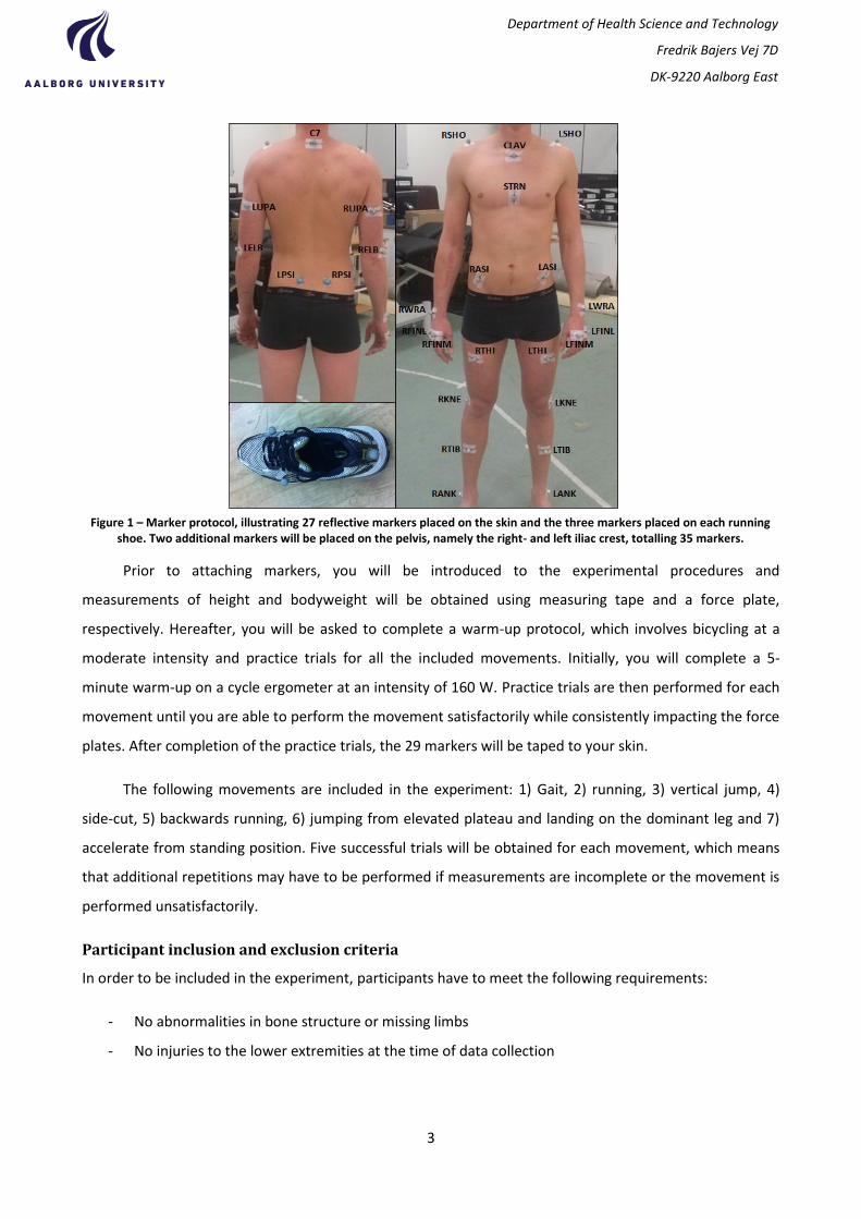
3

Department of Health Science and Technology

Fredrik Bajers Vej 7D

DK-9220 Aalborg East

Prior to attaching markers, you will be introduced to the experimental procedures and

measurements of height and bodyweight will be obtained using measuring tape and a force plate,

respectively. Hereafter, you will be asked to complete a warm-up protocol, which involves bicycling at a

moderate intensity and practice trials for all the included movements. Initially, you will complete a 5-

minute warm-up on a cycle ergometer at an intensity of 160 W. Practice trials are then performed for each

movement until you are able to perform the movement satisfactorily while consistently impacting the force

plates. After completion of the practice trials, the 29 markers will be taped to your skin.

The following movements are included in the experiment: 1) Gait, 2) running, 3) vertical jump, 4)

side-cut, 5) backwards running, 6) jumping from elevated plateau and landing on the dominant leg and 7)

accelerate from standing position. Five successful trials will be obtained for each movement, which means

that additional repetitions may have to be performed if measurements are incomplete or the movement is

performed unsatisfactorily.

Participant inclusion and exclusion criteria

In order to be included in the experiment, participants have to meet the following requirements:

- No abnormalities in bone structure or missing limbs

- No injuries to the lower extremities at the time of data collection

Figure 1 – Marker protocol, illustrating 27 reflective markers placed on the skin and the three markers placed on each running shoe. Two additional markers will be placed on the pelvis, namely the right- and left iliac crest, totalling 35 markers.

4

Department of Health Science and Technology

Fredrik Bajers Vej 7D

DK-9220 Aalborg East

Risks or disadvantages

The majority of the movements included in the study are considered highly dynamic, which means that

they are executed at a high velocity and involves forceful ground impacts and sudden changes in direction.

However, each trial has a very short duration and will be performed under controlled circumstances and

constant supervision. It is assessed that there are no considerable risks or disadvantages associated with

your participation. Your comfort and wellbeing will at all times take precedence over the research.

Anonymity

The personal information collected from you, which includes gender, age, height and weight, will not be

shared in any way. Your information will be de-identified with a code number, which will be used for any

publication purposes. The information that is obtained in connection with this study and can be identified

with you will remain strictly confidential and will be disclosed only with your permission.

Accessibility and publication

The data collected will be included in a Master’s thesis, which will be made accessible to the public through

Aalborg University. Additionally, the results of the study can potentially be published as an article in a

scientific journal and/or conference.

Benefits associated with participation

You will not receive any compensation for your participation. While the results of this research may benefit

the scientific community, we cannot guarantee that you will receive any personal direct benefits.

Participant rights

Your participation is wholly voluntary and you are free to withdraw your consent and to discontinue

participation at any time without prejudice. We will not take responsibility for any accidental injury or

discomfort you may experience during the experiment.

Practical information

We kindly ask that you bring a pair of running tights, if accessible, a t-shirt and towel. Female participants

will need to bring a sports brassiere. In case you are not able to bring your own, two pairs of tights will be

made available for you, however, these may not be of an appropriate size. In addition, we recommend that

you bring a water bottle for your own comfort, as the experiment may take up to two hours.

5

Department of Health Science and Technology

Fredrik Bajers Vej 7D

DK-9220 Aalborg East

Consent form

Participant name:

______________________________________________

I acknowledge that

1) I have read and understood the information provided to me in this document and agree to the

general purpose, methods and demands of the study.

2) The project is for the purpose of research and may not be of direct benefit to me.

3) I have been informed that I am free to withdraw from the study at any time without prejudice.

4) My personal information will be treated anonymously and will be disclosed only with my

permission.

5) The results of the study will be published by Aalborg University and may, additionally, be

published in a scientific journal and/or conference.

6) Participation is wholly voluntary and I will not receive any compensation.

7) I hereby give consent to participate in the study and I am aware that participation is at my own

risk.

Participant: Date:

(Signature)

Investigator: Date:

(Signature)