prediction of freight growth report final - ternz of new zealand's freight gr… · prediction...

Prediction of New Zealand’s freight growth by 2020

80

90

100

110

120

130

140

150

160

170

1999 2000 2001 2002 2003 2004

relative change HVkm (base 1999)

Ireland

Spain

NZ

Europe*

Germany

UK

Prepared for: E. J. Brenan Memorial Trust

Prepared by: Hamish Mackie, Peter Baas, Hansjörg Manz

March 2006

Table of Contents

Executive summary 3

Introduction 4

1. Prediction of road freight growth to 2020 4 1.1 Number of heavy vehicles and kilometres travelled 4 1.2 Confirmation of relationship between heavy vehicle traffic and RGDP 7 1.3 RGDP lags heavy vehicle travel by 1 year. 8 1.4 Incorporating the RGDP lag into the freight prediction model 9 1.5 Using Road User Charges revenue to predict freight growth 10 1.6 Predicted freight growth to 2020 12 1.7 New Zealand’s heavy vehicle travel trend different to other countries 14

2. Prediction of regional heavy vehicle travel to 2020 23 2.1 Regional economic variation 23 2.2 Estimating regional heavy vehicle travel 24

3. Prediction of heavy vehicle travel to 2020 by commodity group 25

4. Factors that may effect freight transport growth in the future 27

References 29 Transport Engineering Research NZ Ltd. Phone: (09) 2622 556 Fax (09) 2622 856 PO Box 97846 South Auckland Mail Centre 17-19 Gladding Pl, Manukau City E-mail: [email protected]

Prediction of freight growth to 2020

3

Executive summary

The purpose of this report is to predict the overall demand for freight transport in New Zealand by 2020 and provide details of freight growth in the nation’s regions and major business sectors.

Road User Charges (RUC) data were used to estimate the number of heavy vehicles (4 tonne and over) and the heavy vehicle distance travelled between 1997 and 2005. This information was used to refine a previously published model that describes the relationship between Real Gross Domestic Product (RGDP) and heavy vehicle kilometres (HVkm) travelled. In addition a model that describes the relationship between RGDP and RUC revenue was developed. The models were then used to provide an estimate for the predicted road freight task by 2020. The relationship between RGDP and heavy vehicle travel was also compared with other countries. Using regional economic data, the model was also applied to New Zealand’s regions in order to estimate heavy vehicle travel at a regional level. Finally, industry production statistics were used to provide an estimate of the transport requirements of a selection New Zealand’s largest commodity groups.

Between 1997 and 2005, the number of heavy vehicles in New Zealand has grown steadily (55% increase for trucks only) with a corresponding increase in HVkm (42%). Previously heavy vehicle travel has been shown to increase at a rate 1.5 times greater than RGDP increases. By adding more recent data the HVkm multiplier (T) has been adjusted to 1.42 if RGDP and heavy vehicle travel are compared in the same year, and 1.35 if a 1 year offset between heavy vehicle travel and RGDP is considered. RUC revenue growth appears to grow slightly faster than HVkm (1.51), which seems to be a result of higher heavy vehicle RUC weights being purchased. If current trends persist, HVkms are predicted to grow by 85% by 2020 and RUC revenue is expected to grow by 93%. Therefore, the road freight task is also expected to also grow by this magnitude.

In comparison, RGDP in many other countries is growing at a faster rate than heavy vehicle travel growth. Also, New Zealand’s heavy vehicle travel is growing at a faster rate than countries such as the USA, UK and many parts of Western Europe. Exceptions to this include Spain and Ireland. At a regional level, large increases in heavy vehicle travel are expected in the Auckland (467 million HVkm), Waikato (565 million HVkm), Bay of Plenty (356 million HVkm) and Canterbury (274 million HVkm) regions by 2020. In the longer term, dairy and forestry production are expected to grow in line with RGDP while the construction industry is expected to grow faster than RGDP in the long-term. The meat industry production is not expected to grow at all by 2020 given current trends.

There are a number of factors that may cause variation from these predictions. The nation’s economy may perform differently from what is expected, as might regional economies. Also, the relationship between freight transport and RGDP might change over time, as our economy becomes more service-oriented and less production-reliant. Alternatively, the current trend for transport to and from increasingly large distribution centres may mean increased transport growth in the future. Traffic congestion – and subsequent road pricing - and fuel costs may also affect the pattern of heavy vehicle growth in the future.


4

Introduction The purpose of this report is to predict the overall demand for freight transport in New Zealand by 2020 and provide details of freight growth in the nation’s regions and major business sectors. The report also provides an update on the key information reported by Bolitho et al. (2003) – Heavy Vehicle Movements in New Zealand. The main benefits from the information in this report include:

• Improved knowledge of future freight volume.

• Improved ability to make planning decisions based on knowledge of predicted freight volume.

• Improved government policy making in the heavy transport sector and the wider transport sector.

There are three main parts to this report:

1. A prediction of overall heavy vehicle travel and RUC revenue to 2020, including a discussion of the methodology used and comparisons with trends from other countries.

2. Predictions to 2020 for freight growth in New Zealand’s regions and the major freight sectors and industries, including a discussion of the methodology that was used.

3. A brief discussion of the factors that may affect freight predictions, including scenarios

that may lead to greater or less overall freight growth in the future.

1. Prediction of road freight growth to 2020

1.1 Number of heavy vehicles and kilometres travelled

Road User Charges (RUC) data were used to estimate the number of heavy vehicles (4 tonne and over, including buses) and the heavy vehicle distance travelled between 1997 and 2005. This analysis is a continuation of previous analyses by Baas and Arnold (1999), Bolitho et al. (2003) and Mueller and Baas (2004) . Buses are included in this analysis. In 2005 there were a total of 102,201 trucks and 22,861 trailers purchasing RUCs. Between 1997 and 2005 the total number of trucks experienced 33% growth while the total number of trailers experienced 18% growth (Figure 1). It appears that growth between 2001 and 2005 was more rapid than between 1997 and 2001. This reflects the more buoyant economic conditions that existed in New Zealand in the latter half of this period.


5

0

20,000

40,000

60,000

80,000

100,000

1997 1998 1999 2000 2001 2002 2003 2004 2005

Number of vehicles

Trucks

Trailers

Figure 1. Number of trucks and trailers between 1997 and 2005, 4 tonne and over (including buses).

Figure 1 shows that there are many more trucks than trailers, meaning that there are a large number of truck-only vehicles (approximately 60% of the fleet). Also, absolute truck growth has been greater than absolute trailer growth. This may reflect the growing need for intra regional general freight and freight between neighbouring regions where time-sensitive loads mean smaller, more frequent loads within these areas. However, Figure 2 shows that truck and trailer combinations demonstrated the largest proportional vehicle km growth between 1997 and 2005 with other combination vehicle types showing less growth. This may reflect the relatively strong economic performance of the primary commodity sector as a whole during this period, along with increased line-haul freight services. Milk, stock, logs and long distance general freight are all mainly transported using truck-trailer combinations. Also, increased centralisation of the processing of primary commodities and more centralised freight distribution would mean that truck-trailer combinations would increasingly need to travel further distances. The single most prevalent type of truck is the 7-10 tonne, 2-axle truck (Table 1). In 2005 there were 19,078 of these vehicles and they accounted for 19% of all trucks. This reflects the large amount of intra-regional freight that takes place, which requires smaller but more frequent and timely delivery of freight. The most common larger trucks were three-axle, 16-20 tonne trucks. The most common trailers in 2005 were 4-axle trailers weighing 21-25 tonne. Table 2 shows that the 3-axle 16-20 tonne trucks travelled the greatest number of kilometres in 2005 (535 million kms). This was followed closely by 4-axle 21-25 tonne trucks (475 million kms). Although there are significantly fewer larger trucks than smaller trucks, the distance they travel each year is significantly greater than smaller trucks (Table 2). Of the trailers, four-axle 21-25 tonne trailers cumulatively travelled the greatest number of kms in 2005 (423 million kms). In part this reflects the fact that they represent the greatest number of trailers, but the average annual distance travelled for these vehicles is also higher than that for other trailers.


6

0

200

400

600

800

1000

1200

1400

1600

1800

2000

1997 1998 1999 2000 2001 2002 2003 2004 2005

HVkm travelled (million)

Truck only

Truck-trailer

Tractor-semi

B-train

Figure 2. Growth in distance travelled by heavy vehicle combinations between 1997 and 2005

Table 1. Numbers of heavy vehicle by weight and RUC vehicle type in 2005.

Table 2. Heavy vehicle kilometres travelled (million) by weight and RUC vehicle type in 2005

Weight 1 2 5 6 14 19 24 27 28 29 30 33 37 43

4 9778 10430 6 24 0 0 41 11 32 29 13 0 1 05 1320 12807 266 34 1 0 76 15 55 61 9 7 6 26 338 7673 20 24 0 0 100 33 32 75 36 30 14 237-10 429 19078 19 345 27 0 251 78 102 1364 232 297 79 15411-15 269 11107 467 1765 454 0 18 14 83 2499 866 757 312 22516-20 10 55 579 10953 1380 1 1 0 5 355 320 3612 1828 88421-25 2 5 26 5872 5972 1 0 0 6 11 1 483 1373 582726-30 2 0 0 26 625 11 0 0 2 2 0 9 53 44

Total 12149 61155 1382 19043 8460 13 487 150 317 4396 1476 5195 3665 7159

RUC type

Trucks / tractors Trailers

Weight 1 2 5 6 14 19 24 27 28 29 30 33 37 43

4 222 153 0 0 0 0 1 0 1 1 0 0 0 0

5 22 213 3 1 0 0 2 0 0 2 0 0 0 0

6 5 135 0 0 0 0 2 0 0 3 1 1 1 0

7-10 6 395 0 7 0 0 3 1 2 101 4 15 2 5

11-15 2 251 24 75 16 0 0 0 2 86 9 51 14 12

16-20 0 1 37 535 72 0 0 0 0 7 4 197 71 66

21-25 0 0 1 228 475 0 0 0 0 0 0 16 39 42326-30 0 0 0 0 26 0 0 0 0 0 0 0 2 1

Total 257 1148 66 846 590 0 8 1 5 200 19 280 129 507

Trucks / tractors Trailers

RUC type


7

1.2 Confirmation of relationship between heavy vehicle traffic and RGDP

A relationship between heavy vehicle travel and real gross domestic product1 (RGDP) was reported by Bolitho et al. (2003). The data used by Bolitho et al. have been updated to include data from 2002-2005 inclusive (Table 4)2. One change to the methodology used to process these updated data was to calculate the total number of heavy vehicle-kms travelled using only trucks, whereas previously the sum of all trucks and trailers were used. While it is accepted that over time there may be a change in the distribution of truck-trailer types, the main predictor of overall heavy vehicle traffic volume is the distance travelled by trucks. This change in methodology resulted in an improvement in the correlation between heavy vehicle movements and RGDP from R2 = 0.73 using truck and trailer data to R2 = 0.90 using truck-only data. A correlation coefficient (R2) that equals 1 represents a perfect linear relationship between two variables, while 0 represents no relationship at all between two variables. By adding the 2002-2005 data, a further improvement in the correlation between heavy vehicle movement and RGDP was observed (R2 = 0.985 – Figure 3), with the ‘transport factor’ (T) reducing slightly to 1.42. Previously, Bolitho et al. (2003) had reported a transport factor of 1.53.

RGDP

(million $) HVkm (million)

1997 95,947 2,042

1998 98,138 2,044

1999 98,556 2,171

2000 103,745 2,257

2001 105,975 2,367

2002 110,147 2,511

2003 115,290 2,619

2004 119,401 2,810

2005 123,841 2,907

Table 3. Real Gross Domestic Product (RGDP) and heavy vehicle kilometres travelled between 1997 and 2005.

1 GDP is the total market value of goods and services produces within a given period after deducting the cost of goods utilised in the process of production. RGDP is expressed as the dollar values of a particular year. RGDP is effectively GDP after adjustment for inflation (NZ Institute of Economic Research http://www.nzier.org.nz/SITE_Default/SITE_economics_explained/GDP.asp).

2 1998-2005 RGDP data: Statistics New Zealand: http://www2.stats.govt.nz/domino/external/pasfull/pasfull.nsf/0/4c2567ef00247c6acc2570de001a51db/$FILE/alltabls.xls. Last accessed 21/03/06. 1997 RGDP data: http://www2.stats.govt.nz/domino/external/pasfull/pasfull.nsf/0/4c2567ef00247c6acc256f710009ac75/$FILE/alltabls.xls. Last accessed 21/03/06.


8

y = 0.0002x1.4226

R2 = 0.9849

1,900

2,100

2,300

2,500

2,700

2,900

3,100

90000 100000 110000 120000 130000

RGDP ($ million)

kilometres travelled

(millions)

Figure 3. Heavy vehicle kilometres travelled vs Real Gross Domestic Product 1997-2005.

1.3 RGDP lags heavy vehicle travel by 1 year.

It appears that changes in RGDP growth lag changes in heavy vehicle travel growth by approximately 1 year (Figure 4). This suggests that increases in RGDP follow increases in heavy vehicle travel. The mechanism for this effect is presumably that after goods and services are produced it takes some time for the revenues to flow back into the economy and be spent at which time they are recorded as contributing to RGDP. This observation suggests that RUC data could be used to predict changes in RGDP for the following year, which may be of benefit to economic forecasters. However, caution needs to be employed as a causal link between RGDP and heavy vehicle travel has not been proved, and the relationship that has been observed has not been tested during periods of recession.

0.0

1.0

2.0

3.0

4.0

5.0

6.0

7.0

8.0

1997 1998 1999 2000 2001 2002 2003 2004

%changeHVkm

% changeRGDP

1998 1999 2000 2001 2002 2003 2004 2005

HVkm

RGDP

Figure 4. Percentage change in heavy vehicle travel and RGDP, with RGDP moved back by one year.


9

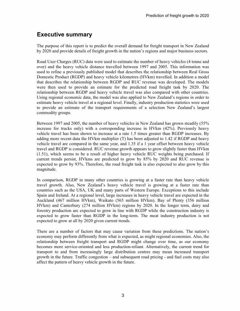
1.4 Incorporating the RGDP lag into the freight prediction model

When the lag in RGDP is incorporated into the freight prediction model an even better fit occurs (R2 = 0.996). Figure 5 shows how off-setting RGDP and heavy vehicle travel data by one year eliminates the variation in this relationship that occurred during New Zealand’s relatively poor economic performance of 1999. However, using this model, the relationship between RGDP and heavy vehicle travel growth is lower (1.35) than was reported previously by Bolitho et al. (T=1.5). This means that, overall, the rate of heavy vehicle growth is slightly less than was previously predicted. The reason for this is mostly that we now have more data to make more robust analyses. Also, over time, Treasury revise previous RGDP figures, which can also slightly affect this relationship. Nevertheless, the main point is that heavy vehicle travel has been growing consistently faster than RGDP.

y = 0.0004x1.3467

R2 = 0.9964

1900

2000

2100

2200

2300

2400

2500

2600

2700

2800

2900

95000 100000 105000 110000 115000 120000 125000

RGDP ($ Millions)

Kilometres travelled (Million)

Figure 5. Heavy vehicle kilometres travelled vs Real Gross Domestic Product 1997-2005, including one year offset

between heavy vehicle travel and RGDP.

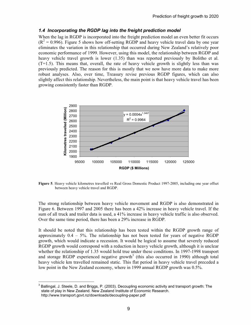
The strong relationship between heavy vehicle movement and RGDP is also demonstrated in Figure 6. Between 1997 and 2005 there has been a 42% increase in heavy vehicle travel. If the sum of all truck and trailer data is used, a 41% increase in heavy vehicle traffic is also observed. Over the same time period, there has been a 29% increase in RGDP. It should be noted that this relationship has been tested within the RGDP growth range of approximately 0.4 – 5%. The relationship has not been tested for years of negative RGDP growth, which would indicate a recession. It would be logical to assume that severely reduced RGDP growth would correspond with a reduction in heavy vehicle growth, although it is unclear whether the relationship of 1.35 would hold true under these conditions. In 1997-1998 transport and storage RGDP experienced negative growth3 (this also occurred in 1990) although total heavy vehicle km travelled remained static. This flat period in heavy vehicle travel preceded a low point in the New Zealand economy, where in 1999 annual RGDP growth was 0.5%.

3 Ballingal, J. Steele, D. and Briggs, P. (2003). Decoupling economic activity and transport growth: The state of play in New Zealand. New Zealand Institute of Economic Research. http://www.transport.govt.nz/downloads/decoupling-paper.pdf


10

The low heavy vehicle travel growth in 1998 followed by the low RGDP growth in 1999 does give some indication of how the relationship between RGDP and heavy vehicle travel growth may be affected during times of recession or poor economic performance. In Figure 3, the 1998 (second from left) data point is significantly lower than the trend line, indicating a relative reduction in heavy vehicle travel compared to RGDP. If this trend were to continue an overall relationship between RGDP and heavy vehicle travel much lower than 1.4 would result. However, in 1999 RGDP growth was low relative to heavy vehicle travel, making this data point much higher than the overall trend line. The net result is that over a two-year period the negative and positive variation in this relationship cancel each other out and a reasonably steady relationship between RGDP and heavy vehicle travel growth of approximately 1.4 is maintained (not accounting for the time off-set between heavy vehicle travel and RGDP). Accounting for the off-set between heavy vehicle travel and RGDP, a HVkm multiplier (T) of 1.35 occurs, although the effect of this off-set is likely to diminish over time as more data points are collected and the influence of the end points are reduced.

1,500

1,700

1,900

2,100

2,300

2,500

2,700

2,900

1997 1998 1999 2000 2001 2002 2003 2004 2005

kilometres travelled (millions)

80000

90000

100000

110000

120000

130000

140000

GDP ($million)

HVKm RGDP

Figure 6. Absolute heavy vehicle travel and RGDP 1997-2005

1.5 Using Road User Charges revenue to predict freight growth

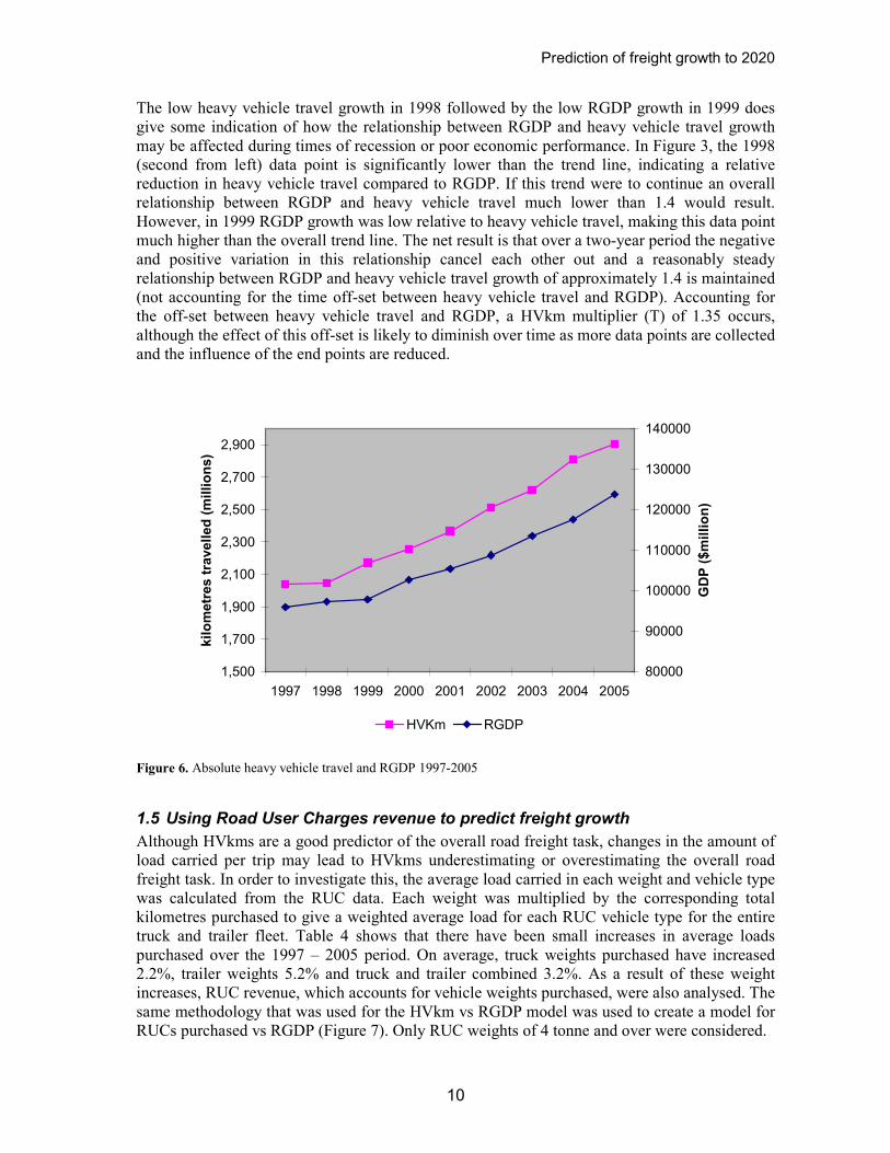
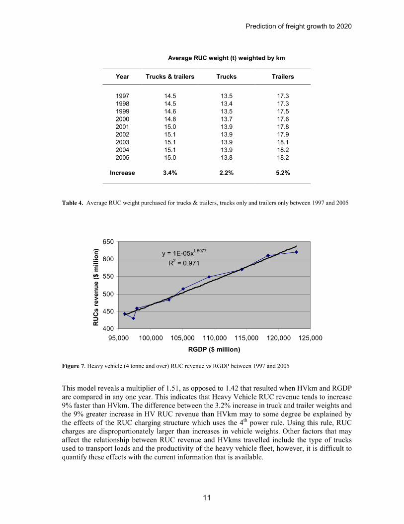
Although HVkms are a good predictor of the overall road freight task, changes in the amount of load carried per trip may lead to HVkms underestimating or overestimating the overall road freight task. In order to investigate this, the average load carried in each weight and vehicle type was calculated from the RUC data. Each weight was multiplied by the corresponding total kilometres purchased to give a weighted average load for each RUC vehicle type for the entire truck and trailer fleet. Table 4 shows that there have been small increases in average loads purchased over the 1997 – 2005 period. On average, truck weights purchased have increased 2.2%, trailer weights 5.2% and truck and trailer combined 3.2%. As a result of these weight increases, RUC revenue, which accounts for vehicle weights purchased, were also analysed. The same methodology that was used for the HVkm vs RGDP model was used to create a model for RUCs purchased vs RGDP (Figure 7). Only RUC weights of 4 tonne and over were considered.


11

Average RUC weight (t) weighted by km

Year Trucks & trailers Trucks Trailers

1997 14.5 13.5 17.3

1998 14.5 13.4 17.3

1999 14.6 13.5 17.5

2000 14.8 13.7 17.6

2001 15.0 13.9 17.8

2002 15.1 13.9 17.9

2003 15.1 13.9 18.1

2004 15.1 13.9 18.2

2005 15.0 13.8 18.2

Increase 3.4% 2.2% 5.2%

Table 4. Average RUC weight purchased for trucks & trailers, trucks only and trailers only between 1997 and 2005

y = 1E-05x1.5077

R2 = 0.971

400

450

500

550

600

650

95,000 100,000 105,000 110,000 115,000 120,000 125,000

RGDP ($ million)

RUCs revenue ($ m

illion)

Figure 7. Heavy vehicle (4 tonne and over) RUC revenue vs RGDP between 1997 and 2005

This model reveals a multiplier of 1.51, as opposed to 1.42 that resulted when HVkm and RGDP are compared in any one year. This indicates that Heavy Vehicle RUC revenue tends to increase 9% faster than HVkm. The difference between the 3.2% increase in truck and trailer weights and the 9% greater increase in HV RUC revenue than HVkm may to some degree be explained by the effects of the RUC charging structure which uses the 4th power rule. Using this rule, RUC charges are disproportionately larger than increases in vehicle weights. Other factors that may affect the relationship between RUC revenue and HVkms travelled include the type of trucks used to transport loads and the productivity of the heavy vehicle fleet, however, it is difficult to quantify these effects with the current information that is available.


12

Based on the present findings, it is likely that the growth in road freight relative to RGDP growth is higher than 1.42 (HVkm vs RGDP for any one year) but lower than 1.51 (HV RUC revenue vs RGDP). Because RUC data tell us nothing about the percentage vehicle utilisation that is occurring, we are unable to determine whether this has changed over time. Freight transport operators may be increasing their vehicle utilisation over time in order to improve productivity, although for operators who are carrying out ‘just in time’ deliveries, this may be difficult to achieve as trucks may need to travel with partial loads in order to meet deadlines. However, the increase in vehicle weights purchased over time hints that payloads per trip have increased, assuming that operators are trying to load trucks as close as possible to RUC weights purchased all of the time (actual loads = RUC weights purchased). This would result in relatively more freight being carried relative to HVkm, and would be reflected in disproportionately higher RUC revenue growth relative to HVkm growth.

1.6 Predicted freight growth to 2020

Given that heavy vehicle travel and HV RUC revenue growth has such a strong association with RGDP growth, predicting RGDP growth to 2020 is the best way of predicting overall heavy vehicle travel and road freight growth. Bolitho et al. (2003) also examined the relationship between heavy vehicle travel and population growth but found a very poor relationship between them. (R2 = 0.175).

One of the roles of the Treasury is to forecast RGDP among other economic indicators. In the Treasury’s pre-election economic and fiscal update 2005, forecasts are given for RGDP until 20094. Growth in RGDP is expected to slow to 2.2% in the March 2006 year and 2.6% in the March 2007 year. The delayed effects of high exchange and interest rates, a continued slowing in net migration inflows, slower trading partner growth over 2005 and a forecast decline in the terms of trade are given as the main contributors to this slow-down. Following this, Government spending and investment are expected to make a positive contribution to RGDP growth along with export growth in 2007. However, weak residential investment growth will result in overall RGDP growth remaining relatively muted.

RGDP growth is then forecast to pick up to 3.5% in the March 2008 year and 3.1% in the March 2009 year. Underlying this pick-up is robust export growth following its recovery in the March 2007 year. Also, improved private spending growth, due to increasing labour and export incomes and a projected fall in interest rates, is also expected to contribute to the recovery. This will also be helped by improved residential investment growth as the decline in residential investment is expected to end. Throughout this time, import growth is expected to remain relatively low due to the low New Zealand dollar exchange rate.

No forecasts could be found for RGDP beyond 2009. However, the average RGDP growth from 1995-2005 has been 3.5%, which includes periods of high growth and a period of low growth around the turn of the millennium, largely as a result of reduced trading with Asian countries, and a large drought in the summers of 1997/98 and 1998/99. Being slightly more conservative than the RGDP growth of the last ten years, it would be reasonable to fix RGDP growth at 3.0% for the period 2010-2020. Using these figures, and the ‘same year’ HVkm multiplier (T) of 1.42 for heavy vehicle travel and 1.51 for RUC revenue, a forecast for road freight growth to 2020 can be made (Figure 8).

4 The Treasury, pre-election and fiscal update 2005, http://www.treasury.govt.nz/forecasts/prefu/2005/1economic.asp


13

Using this model, an 85% increase in heavy vehicle travel is expected for the 15 years between 2005 and 2020. This would mean an increase in HVkm from 2,907 million HVkm in 2005 to 5,390 HVkm in 2020. Because much of this time uses a fixed estimated RGDP growth of 3.0%, it is prudent to examine the effects of differing scenarios:

• If RGDP growth between 2010 and 2020 were less than expected and fixed at 2.5%, then there would be a corresponding increase in heavy vehicle travel of 72% (between 2005 and 2020). This would mean in increase in HVkm from 2,907 million HVkm in 2005 to 5,034 HVkm in 2020.

• If RGDP growth continues as it has done for the last ten years and is fixed at 3.5% between 2010 and 2020, then there would be a corresponding increase in heavy vehicle travel of 100% (between 2005 and 2020). This would mean an increase in HVkm from 2,907 million HVkm in 2005 to 5,808 HVkm in 2020.

Using the RUC revenue model, a 93% increase in RUC revenue is expected for the 15 years between 2005 and 2020. This would mean an increase in RUC revenue from $621m in 2005 to $1,196m in 2020.

• If RGDP growth between 2010 and 2020 were less than expected and fixed at 2.5%, then there would be a corresponding increase in RUC revenue of 78% (between 2005 and 2020). This would mean an increase in RUC revenue from $621m in 2005 to $1,104m in 2020.

• If RGDP growth continues as it has done for the last ten years and is fixed at 3.5% between 2010 and 2020, then there would be a corresponding increase in RUC revenue of 109% (between 2005 and 2020). This would mean an increase in RUC revenue from $621m in 2005 to $1,294m in 2020.

These projections mean that the growth in the total freight task is likely to be between 72% and 109% using reasonable upper and lower RGDP growth figures for HVkms growth as a lower freight growth estimate and RUC revenue growth as an upper freight growth estimate. This does not include errors associated with estimating RGDP and the confidence intervals of the HVkm and RUC revenue models. However, the 95% confidence intervals for HVkm and RUC revenue growth are very similar in magnitude to the intervals created using 2.5% and 3.5% RGDP growth. Figure 8 shows predicted HVkm and RUC revenue growth from 2005, and their associated 95% confidence intervals.

There is obviously some error associated with forecasting RGDP and attempting to predict heavy vehicle travel from this. The forecast 2005 RGDP figure used by Bolitho et al. (2003) – based on actual RGDP from 1997 up to and including 2001, was compared with the actual RGDP for 2005. There was a 3.3% difference between the actual and estimated RGDP for 2005, which equates to a difference in vehicle travel of 4.46%, or approximately one year of typical heavy vehicle growth.


14

0

10

20

30

40

50

60

70

80

90

100

110

2005 2007 2009 2011 2013 2015 2017 2019

Year

Percent growth from 2005

RUC rev upper

RUC rev est.

RUC rev lower

HVKm upper

HVKm est.

HVKm lower

Figure 8. Estimated HVKm and RUC revenue growth between 2005 and 2020. The solid lines represent the predicted growth from the models and the dotted lines represent the upper and lower bounds for the confidence intervals.

Figure 8 clearly shows that there is considerable overlap between the confidence intervals for HVKm and RUC revenue growth. This suggests that we cannot statistically differentiate between the two models. Realistically, either growth in HVkm or RUC revenue could be used to estimate road freight growth, especially as we are not currently able to measure actual vehicle weights and the percentage utilisation of heavy vehicles.

1.7 New Zealand’s heavy vehicle travel trend different to other countries

It appears that the relationship between RGDP and heavy vehicle travel that exists for New Zealand does not exist for many other countries, although a factor of 1.5 has been reported in Europe where a 1% increase in industrial production leads to a 1.5% rise in road transport (Meersman and Van der Voorde 1999). Figure 9 shows the change in heavy vehicle travel (HVkm), the change in RGDP and the change in the ratio HVkm/RGDP for New Zealand between 1997 and 20055. Each variable has been standardised to a base of 100 at 1997 so that their relative changes can be compared. The ratio HVkm/RGDP is often calculated as it gives an indication of ‘transport intensity’ or the amount of transport that is required to grow the economy of a country by a given amount. As would be expected, because the change in heavy vehicle travel is increasing at a rate of approximately 1.42 times the change in RGDP, the ratio HVkm/RGDP has also increased between 1997 and 2005. However, a different trend is shown

5 Calculated from data used in earlier analysis of HVkm multiplier factor (T).


15

by Figure 10, which shows the same variables for the UK6. In the UK heavy vehicle travel (HVkm) has only increased slightly (and more recently decreased) while RGDP has increased steadily. Correspondingly, the ratio HVkm/RGDP has decreased from 100 to 78 between 1997 and 2004. A similar, yet less pronounced pattern is shown for the USA7 (Figure 11), where RGDP has grown at a faster rate than road HVkms in recent years, yet has been almost equal in previous years. It appears that the UK, and to a lesser degree the USA, have been able to grow their economies with disproportionately less growth in heavy vehicle travel.

90

100

110

120

130

140

150

1997 1998 1999 2000 2001 2002 2003 2004 2005

relative change (base 1997)

HVKm

RGDP

HVKm/RGDP

Figure 9. Relative change in heavy vehicle km (HVkm), RGDP and the ratio HVKm/RGDP for New Zealand between 1997 and 2005.

6 Data calculated from Department for Transport spreadsheet: Domestic Freight Transport by Mode 1953-2004 http://www.dft.gov.uk/stellent/groups/dft_transstats/documents/divisionhomepage/037806.hcsp

7 Calculated using sum of freight vehicles km travelled. Beureau of Transportation Statistics. http://www.bts.gov/publications/national_transportation_statistics/2005/excel/table_01_32_m.xls


16

70

80

90

100

110

120

130

1996 1997 1998 1999 2000 2001 2002 2003 2004


HVKm

RGDP

HVKm/RGDP

Figure 10. Relative change in heavy vehicle km (HVkm), RGDP and the ratio HVKm/RGDP for the UK between

1996 and 2004.

95

100

105

110

115

120

125

130

135

1994 1995 1996 1997 1998 1999 2000 2001 2002

relative change (base = 1994)

HVkm

GDP

HVkm/RGDP

Figure 11. Relative change in heavy vehicle km (HVkm), RGDP and the ratio HVkm/RGDP for the USA between

1994 and 2002.

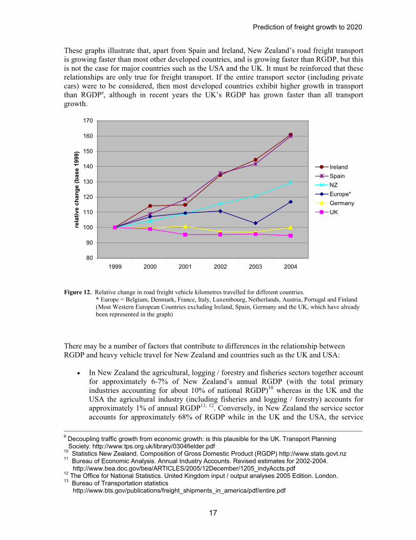
A comparison in the growth of road freight transport (HVkm) between different countries is shown in Figure 128. New Zealand’s road freight transport has grown much faster than many European countries, especially in recent years. However, exceptions to this include Ireland and Spain. These countries have demonstrated phenomenal growth in road freight transport. Although Ireland’s RGDP growth has averaged approximately 6.1% per annum over this period, transport growth has been much higher.

8 Eurostat. http://epp.eurostat.cec.eu.int


17

These graphs illustrate that, apart from Spain and Ireland, New Zealand’s road freight transport is growing faster than most other developed countries, and is growing faster than RGDP, but this is not the case for major countries such as the USA and the UK. It must be reinforced that these relationships are only true for freight transport. If the entire transport sector (including private cars) were to be considered, then most developed countries exhibit higher growth in transport than RGDP9, although in recent years the UK’s RGDP has grown faster than all transport growth.

80

90

100

110

120

130

140

150

160

170

1999 2000 2001 2002 2003 2004


Ireland

Spain

NZ

Europe*

Germany

UK

Figure 12. Relative change in road freight vehicle kilometres travelled for different countries.

* Europe = Belgium, Denmark, France, Italy, Luxembourg, Netherlands, Austria, Portugal and Finland (Most Western European Countries excluding Ireland, Spain, Germany and the UK, which have already been represented in the graph)

There may be a number of factors that contribute to differences in the relationship between RGDP and heavy vehicle travel for New Zealand and countries such as the UK and USA:

• In New Zealand the agricultural, logging / forestry and fisheries sectors together account for approximately 6-7% of New Zealand’s annual RGDP (with the total primary industries accounting for about 10% of national RGDP)10 whereas in the UK and the USA the agricultural industry (including fisheries and logging / forestry) accounts for approximately 1% of annual RGDP11, 12. Conversely, in New Zealand the service sector accounts for approximately 68% of RGDP while in the UK and the USA, the service

9 Decoupling traffic growth from economic growth: is this plausible for the UK. Transport Planning Society. http://www.tps.org.uk/library/0304fielder.pdf

10 Statistics New Zealand. Composition of Gross Domestic Product (RGDP) http://www.stats.govt.nz

11 Bureau of Economic Analysis. Annual Industry Accounts. Revised estimates for 2002-2004. http://www.bea.doc.gov/bea/ARTICLES/2005/12December/1205_indyAccts.pdf

12 The Office for National Statistics. United Kingdom input / output analyses 2005 Edition. London.

13 Bureau of Transportation statistics http://www.bts.gov/publications/freight_shipments_in_america/pdf/entire.pdf


18

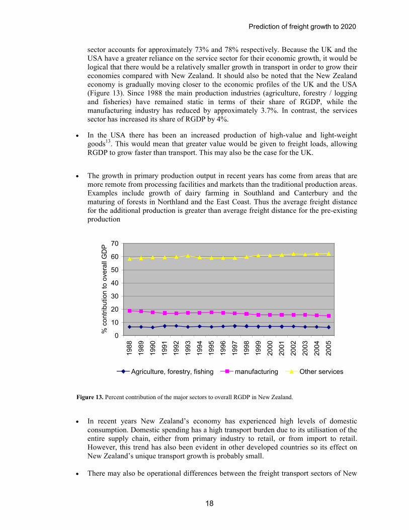
sector accounts for approximately 73% and 78% respectively. Because the UK and the USA have a greater reliance on the service sector for their economic growth, it would be logical that there would be a relatively smaller growth in transport in order to grow their economies compared with New Zealand. It should also be noted that the New Zealand economy is gradually moving closer to the economic profiles of the UK and the USA (Figure 13). Since 1988 the main production industries (agriculture, forestry / logging and fisheries) have remained static in terms of their share of RGDP, while the manufacturing industry has reduced by approximately 3.7%. In contrast, the services sector has increased its share of RGDP by 4%.

• In the USA there has been an increased production of high-value and light-weight goods13. This would mean that greater value would be given to freight loads, allowing RGDP to grow faster than transport. This may also be the case for the UK.

• The growth in primary production output in recent years has come from areas that are more remote from processing facilities and markets than the traditional production areas. Examples include growth of dairy farming in Southland and Canterbury and the maturing of forests in Northland and the East Coast. Thus the average freight distance for the additional production is greater than average freight distance for the pre-existing production

0

10

20

30

40

50

60

70

1988

1989

1990

1991

1992

1993

1994

1995

1996

1997

1998

1999

2000

2001

2002

2003

2004

2005

% contribution to overall GDP

Agriculture, forestry, fishing manufacturing Other services

Figure 13. Percent contribution of the major sectors to overall RGDP in New Zealand.

• In recent years New Zealand’s economy has experienced high levels of domestic consumption. Domestic spending has a high transport burden due to its utilisation of the entire supply chain, either from primary industry to retail, or from import to retail. However, this trend has also been evident in other developed countries so its effect on New Zealand’s unique transport growth is probably small.

• There may also be operational differences between the freight transport sectors of New


19

Zealand and the UK and USA. However, there appears to be no literature available that specifically addresses this.

While the economic profile of New Zealand may never be the same as larger countries such as the UK and USA and may always have a greater reliance on transport due to our relatively large primary sector, it might be that the current relationship between RGDP and heavy vehicle travel changes in the future as New Zealand moves towards a more service and value-added economy. Alternatively, New Zealand is increasingly becoming a distribution centre for overseas manufactured products. Large storage and distribution centres that are emerging in some of New Zealand’s main centres create a large transport requirement, especially in the immediate vicinity of such facilities. Likewise, the possible trend towards port rationalisation means that increasingly, freight will need to be transported longer distances to reach a major port, as opposed to simply travelling to the nearest port. The capacity of New Zealand’s roading network is unlikely to keep pace with the current rate of overall traffic growth, especially in large urban areas. This would mean that the growth of road freight transport might be constrained by congestion in some urban areas in the future. The relative decrease in HVKm in the UK in recent years may be as a result of the substantial congestion that exists on a number of major arterial routes such as the M25 (ring-road around London), the M1 (main motorway north from London) and the M6 (between Birmingham and Manchester). Fortunately, apart from a few instances of holiday traffic, New Zealand’s traffic congestion is generally still limited to urban areas such as Auckland, Tauranga and Hamilton. The problem is that a large proportion of the country’s freight originates or terminates at these centres. The effects of adding value to our commodities on transport are complicated. An example of adding value might be if an increased proportion of our harvested wood were to be used in the manufacturing of wooden furniture. The value of a truckload of furniture is likely to be greater than a similar sized truckload of logs, which would have the effect of increasing the country’s RGDP while decreasing the transport requirement. Conversely, the process of adding value to the wood would require a greater number of transport links and therefore increase the reliance on transport. However, this could be negated to some degree by strategically placing sites that add value to products on routes between primary industry sites and export or retail / distribution sites, effectively minimising the additional transport requirement for added-value products. Pastowski 199714 reported that the effects of more secondary and tertiary production in an economy lead to reduced transport intensity (i.e. higher RGDP growth relative to transport growth). More specifically, a 1% increase in share in the tertiary production sector leads to a 0.3% decrease in transport intensity. Also, more value-added goods tend to be lighter in weight with respect to their value and would therefore require a reduced transport demand. Improved technology may also assist in increasing the value of the commodities that are transported. Fonterra has recently implemented milk-filtering technology in order to reduce its reliance on transport. This will be discussed later in this report, when specific commodity groups are discussed. Further comparisons with other countries are provided in Table 5. Per capita or land area, New Zealand has notable values for the following statistics:

14 Pastowski, A. (1997). Decoupling economic development and freight for reducing its negative impacts; Wuppertal papers, No. 79, Wuppertal Institute for Climate, Environment and Energy.


20

• Gross National Income per capita (second lowest behind Czech Republic)

• Tkm (road) per $1USD of RGDP (third highest behind Czech Republic and Australia)

• Tkm rail per km rail (Third lowest behind Ireland and Japan)

• Tkm road per km road (second lowest behind Australia)

• Km motorway per 1 million inhabitants (second lowest behind Ireland)

• Km motorway per 1000 sqkm (second lowest behind Australia) From the information provided in Table 5, it could be concluded that New Zealand has a relatively low income per capita and a relatively high freight transport intensity (freight transport required to produce a given level of RGDP). New Zealand’s high freight transport intensity is consistent with the earlier finding that demonstrated that road freight HVkms have grown at 1.42 times RGDP (or 1.35 including a one year off-set) over the past eight years. New Zealand also has relatively little freight for its length of road and rail, but overall the road on which freight travels has a relatively low capacity as New Zealand has relatively little motorway. Some other interesting observations from Table 5 include:

• The Czech Republic has the greatest total and road freight transport per $1USD RGDP by a large margin.

• Germany and the UK have approximately three times as much freight (tkm) per km of road as New Zealand.

• A large amount of Japan’s freight (approximately 41%) is transported by coastal shipping. Japan is similar in land area and shape to New Zealand, but has a much larger population.


21

NZ

EU-25

UK

Germ

any France Ireland Czech Rep Austria

Australia

USA

Japan

Largest

lowest

Population (Mill)

4.1

454.6

59.3

82.5

59.8

4.0

10.2

8.1

19.9

290.8

127.6 USA

NZ, IRE

Surface area (1000 sq

km)

271

3900

243

357

552

70

79

84

7700

9600

378

USA,

ASTRL

IRE, AUS

Gross National Income

per capita (current USD) 15530 17071 28320

25270

24750 27020

7190

26810

21960

37870

34190 USA, JAP CZE, NZ

RGDP total (current

1000 Mill USD) 2

80

10973

1800

2400

1800

154

90

253

522

10900

4300

EU-25,

USA

NZ, CZE

Total road length (km)

90000 5224000 412847 628792 987014 95611

127210

104986

8102001

7173000 1172000 USA, EU-

25

NZ

Total motorway length

(km)

170

55957

3609

11786

10068

125

517

1645

1819

89996

5568

USA, EU-

25

IRE

Total railway length (km) 3898 204230 16994

35986

31385

1919

9523

5980

41286

157485 30178 EU-25,

USA

IRE

Inland Freight Transport

Total (Mill tkm) (Coastal

Shipping not included)

16386 2123324 185700 442900 266200 16300

64700

45000

259800

5464400 334000 USA

IRE, NZ

Freight Transport Road

(Mill tkm)

12923 1525452 157000 290900 189200 15900

46600

18100

88400

1534400 312000 USA, EU-

25

NZ, IRE

Freight Transport Rail

(Mill tkm)

3463 355055 18900

78500

46800

400

15800

16900

134100

2200200 23000 USA

IRE, NZ

Freight Transport

Coastal Shipping (Mill

tkm)

3200

- 65900

0

10500

1600

0

0

- 384900 236000 USA

-

Tkm (road, rail, inland

water) per 1 US$ RGDP

(tkm/RGDP)

0.21

0.19

0.10

0.18

0.15

0.11

0.72

0.18

0.50

0.50

0.08

CZE, USA,

AUS

JAP, UK,

IRE

Tkm road per 1 US$

RGDP (tkm/RGDP)

0.16

0.14

0.09

0.12

0.11

0.10

0.52

0.07

0.17

0.14

0.07

CZE, Oz,

NZ

JAP, AUS,

UK

Table 5. Dem

ographic and freight transport comparisons between countries


22

NZ

EU-25

UK

Germ

any France Ireland Czech Rep Austria Australia 1)

USA

Japan

Largest

lowest

Tkm rail per 1 US$

RGDP (tkm/RGDP)

0.04

0.03

0.01

0.03

0.03

0.00

0.17

0.07

0.26

0.20

0.01

AUS, USA IRE, JAP,

UK

Tkm road per capita

3231

3356

2648

3526

3164

3975

4569

2235

4442

5276

2445

USA, CZE AUS, JAP

Tkm rail per capita

866

781

319

952

783

100

1549

2086

6739

7566

180

USA,

ASTRL*

IRE

Mill tkm rail per km rail

0.89

1.74

1.11

2.18

1.49

0.21

1.66

2.83

3.25

13.97

0.76

USA

IRE, JAP,

NZ

Mill tkm road per km

motorway

76

27

44

25

19

127

90

11

49

17

56

IRE, CZE AUS, USA

Mill tkm road per km

road

0.14

0.29

0.38

0.46

0.19

0.17

0.37

0.17

0.11

0.21

0.27

GER, UK ASTRL, NZ

km motorway per 1 mill

inhabitants

43

123

61

143

168

31

51

203

91

309

44

USA

IRE, NZ

km motorway per 1000

sqkm

0.6

14.3

14.9

33.0

18.3

1.8

6.6

19.6

0.2

9.4

14.7

GER

ASTRL, NZ

km total road per 1 mill

inhabitants

22500 11491

6962

7622

16505 23903

12472

12961

40714

24666

9185

ASTRL

UK, GER

km total road per 1000

sqkm

333

1339

1700

1761

1790

1361

1613

1252

105

747

3101

JAP

AUS, NZ

km railway per 1 mill

inhabitants

975

449

287

436

525

480

934

738

2075

542

237

ASTRL

JAP, UK

km railway per 1000

sqkm

14

52

70

101

57

27

121

71

5

16

80

CZE, GER AUSTR, NZ

Table 5. (continued). Dem

ographic and freight transport comparisons between countries

Note: ASTRL = Australia, EU-25 = All members of European Union as of 1 May 2004

1) includes approx. 67000km forestry roads in Vic. & WA, 2) EU 25: 2001, rest 2003

References:

population, surface area, GNI per capita, RGDP:

www.worldbank.org/data -> data -> key statistics on 13 Jan 2006 12.20 pm NZDT (2003) (except EU 25)

www.europe.eu.int on 13 Jan 2006 5.20 pm NZDT (EU 25) (2001)


23

Freight transport total, road, rail, costal shipping:

OECD in Figures - 2005 edition (except NZ) NZ data calculated from: Development of a New Zealand National Freight Matrix (Booz Allen Hamilton (NZ) Ltd, Wellington).

Total length of railway:

epp.eurostat.cec.eu.int on 12 Jan 12.40 pm NZDT (2001, Japan 1994); (except Australia, NZ)

www.abs.gov.au on 13 Jan 5.20 pm NZDT (Australia)

www.tollrail.co.nz on 25 Jan 06 4.20 pm NZDT (NZ)

2. Prediction of regional heavy vehicle travel to 2020

2.1 Regional economic variation

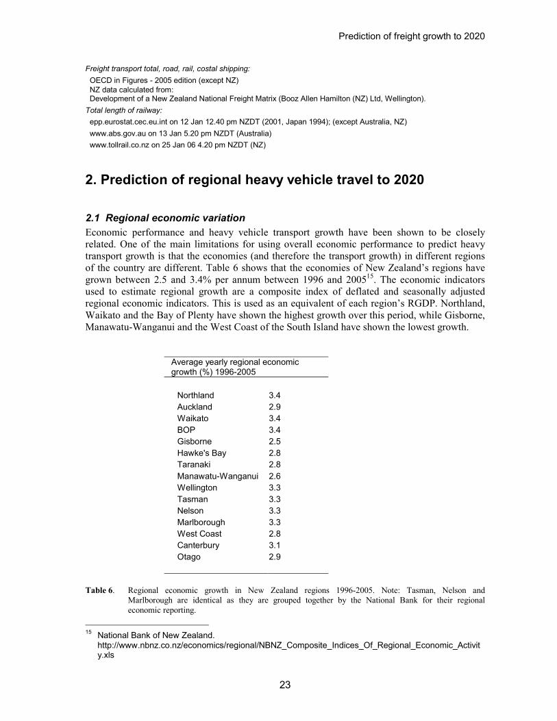
Economic performance and heavy vehicle transport growth have been shown to be closely related. One of the main limitations for using overall economic performance to predict heavy transport growth is that the economies (and therefore the transport growth) in different regions of the country are different. Table 6 shows that the economies of New Zealand’s regions have grown between 2.5 and 3.4% per annum between 1996 and 200515. The economic indicators used to estimate regional growth are a composite index of deflated and seasonally adjusted regional economic indicators. This is used as an equivalent of each region’s RGDP. Northland, Waikato and the Bay of Plenty have shown the highest growth over this period, while Gisborne, Manawatu-Wanganui and the West Coast of the South Island have shown the lowest growth.

Average yearly regional economic growth (%) 1996-2005

Northland 3.4

Auckland 2.9

Waikato 3.4

BOP 3.4

Gisborne 2.5

Hawke's Bay 2.8

Taranaki 2.8

Manawatu-Wanganui 2.6

Wellington 3.3

Tasman 3.3

Nelson 3.3

Marlborough 3.3

West Coast 2.8

Canterbury 3.1

Otago 2.9

Table 6. Regional economic growth in New Zealand regions 1996-2005. Note: Tasman, Nelson and

Marlborough are identical as they are grouped together by the National Bank for their regional economic reporting.

15 National Bank of New Zealand. http://www.nbnz.co.nz/economics/regional/NBNZ_Composite_Indices_Of_Regional_Economic_Activity.xls


24

2.2 Estimating regional heavy vehicle travel

The estimated amount of freight (in tonnes) that moves between and within each region has been calculated by Bolland et al. (2005), using 2002 traffic movements as a base for their estimation. Auckland, Waikato and the Bay of Plenty account for over half of all of New Zealand’s road and rail freight, and the greatest amount of freight tends to be moved within these regions, with Auckland having the largest intra-regional road freight movement (15,333,000 tonnes per year – based on 2002 volumes). The freight matrix also shows that the bulk of cross-regional freight movement occurs between adjoining regions. Using the regional freight estimations by Bolland et al. and the regional economic performance statistics provided by the National Bank, the amount of heavy vehicle traffic within each region can be estimated and predicted to 2020 (Figures 14 & 15), allowing for the following assumptions:

• That the regional freight tonnages reported by Bolland et al. are directly proportional to the heavy vehicle traffic (HVkm) in each region.

• That the regional freight movements reported by Bolland et al. are accurate (the matrix is based on modelling in order to estimate freight movements).

• That each region’s annual average economic growth between 1996-2005 will, on average, be the same as annual average growth between 2005-2020.

• That a transport factor (T) of 1.42 exists (HVKm/RGDP)

• That the regional economic indicators used by the National Bank are closely related to regional RGDP.

0

200

400

600

800

1000

1200

Northland

Auckland

Waikato

BOP

Gisborne

Hawke's Bay

Taranaki

Mana-Wang

Wellington

Tasman

Nelson

Marlborough

West Coast

Canterbury

Otago

Southland

HVKm (million)

2005

2020

Figure 14. Regional heavy vehicle travel growth (HVkm) between 2005 and 2020.


25

0

20

40

60

80

100

120

Northland

Auckland

Waikato

BOP

Gisbourne

Hawke's Bay

Taranaki

Mana-Wang

Wellington

Tasman

Nelson

Marlborough

West Coast

Canterbury

Otago

Southland

% HVkm Growth

Figure 15. Percent heavy vehicle growth between 2005 and 2020 in each region

It is clear from figure 15 that, using this method of prediction, Auckland, Waikato, BOP and Canterbury will have much greater absolute increases in heavy vehicle travel than the other regions. While the Waikato can expect heavy vehicle growth of 104% by 2020, Gisborne can only expect growth of 62%. The Auckland, Waikato, Bay of Plenty triangle, along with the Canterbury region, will experience the greatest increase in heavy vehicle travel of all New Zealand regions. The largest absolute growth in heavy vehicle travel is expected in the Waikato where an increase of 565 million HVkm is expected by 2020. Road User Charges data indicate that on average truck travel distance is approximately 28,000 km (a large combination vehicle typically travels 70,000 km or more per year while the much more numerous urban trucks travel much fewer kms). This would mean that the Waikato region could expect an extra 20,179 heavy vehicle trips by 2020. This gives weight to a rationale for prioritising the improvement of infrastructure within the Auckland, Waikato, Bay of Plenty regions, as well as improving infrastructure within the Canterbury region.

3. Prediction of heavy vehicle travel to 2020 by commodity group

The predicted future growth of our largest primary industries is shown in Figure 1616. For the

dairy and meat industries, MAF predictions were used until 2009, after which the growth rates of previous years were used to project production rates to 2020 for the dairy industry, although growth between 1990 and 2005 has been 3.14% on average, a more conservative 3% was used to account for the limited amount of land that remains for dairying growth. For the forestry

16 Figures calculated from MAF Situation and Outlook for New Zealand Agriculture and Forestry 2005. Construction industry figures were calculated from the Department of building and Housing industry reports. http://www.building.dbh.govt.nz/e/publish/industry-reports.shtml


26

industry, MAF predictions to 2020 were used. Industry reports from the Department of Building and Housing were used to predict future building trends. While the Dairy and Forestry sectors are predicted to grow at a similar rate to RGDP, the meat industry is not expected to grow at all (based on previous trends). Many farms with livestock have been converted into dairy farms, causing growth in dairy but a subdued meat industry. The continued growth in the dairy and forest industries in the long-term is significant as the largest producers of milk and processors and export of wood are in the Waikato and Bay of Plenty regions, which are also the regions that already have a high heavy vehicle traffic volume between and within them. Tauranga port handled 47% of the country’s export logs and 41% of the country’s export sawn timber in 2004. Also, approximately one third of the country’s dairy herds are situated in the South Auckland / Waikato region17. The expected continual growth of dairy and forestry will contribute to the accelerated growth in heavy vehicle traffic that is expected within and between the Waikato and Bay of Plenty regions over the next 15 years.

Although forestry production growth is directly linked proportionally to log and wood product transport, this may not necessarily be the case for milk production. Fonterra is installing milk concentration technology at their Tuamarina site, which will result in 3,000 fewer truck movements a year on the road between Marlborough and South Canterbury18. Presently, milk from Fonterra's Marlborough suppliers is collected by tanker and taken to the Tuamarina site and then transported to the company's Clandeboye site by road for processing. The reverse osmosis plant will filter the milk, with the solids retained and the liquid (water) discarded. This means less volume of milk to transport. The plant is being installed by Tetra Pak New Zealand. This is an example of how technology can be used to reduce the dependence on transport while maintaining productivity and growing the country’s economy.

60

80

100

120

140

160

180

200

2004

2005

2006

2007

2008

2009

2010

2011

2012

2013

2014

2015

2016

2017

2018

2019

2020

relative growth GDP

Milk solidsproduced

Total livestock

Log production

buildingconsents

estimated

forecast

Figure 16. Forecast and estimated growth in New Zealand’s largest commodity groups and the construction

industry between 2005 and 2020.

17 Livestock Improvement Dairy Statistics 2004/2005. http://www.lic.co.nz/pdf/dairy_stats/Dairy_Statistics_05.pdf

18 Fonterra news release, 2

nd Dec, 2005. http://www.fonterra.com/fonterra/content/news/fonterranews


27

The construction industry creates a large amount of intra-regional transport. Timber framing, concrete, appliances, roofing materials, landscaping materials, aggregates and machinery are examples of the products that require transporting between retail and warehouse depots and building sites. Building activity is expected to decline over the next few years and then pick up again at a rate of growth greater than RGDP growth.

4. Factors that may effect freight transport growth in the future

A strong link between New Zealand’s RGDP and truck kilometres travelled has been demonstrated. This means that if New Zealand’s economic growth were to be maintained, then a corresponding growth in heavy vehicle traffic of 1.35 times RGDP can be expected. The nature of this relationship is such that changes in heavy vehicle traffic growth are likely to be more volatile than changes in RGDP. For example, 1% RGDP growth will result in heavy vehicle traffic growth of 1.35%, while 4% RGDP growth will result in 5.4% heavy vehicle traffic growth. In this example, there has been a 3% range in RGDP growth and a 4.05% range in heavy vehicle traffic growth. As mentioned earlier, it is unknown whether the relationship between RGDP and heavy vehicle travel will be maintained during periods of negative RGDP growth. New Zealand last had negative RGDP growth in 1992, and it is feasible that such a period may occur again in the future. There is also error associated with RGDP forecasts and estimations. The Reserve Bank of New Zealand has carried out work to determine the errors associated with RGDP forecasts19. Between 1994 and 2002 RGDP forecasts by the Reserve Bank have been on average 0.25 percentage points higher than actual RGDP. This would mean that the estimations for heavy vehicle travel in the future may be slightly higher than what will eventuate.

In a recent survey of freight operators within Auckland20, 81% of respondents reported experiencing delays due to congestion of over 50 minutes per day and 53% reported congestion related delays of over 1.5 hours. Congestion was also cited as the single biggest issue currently facing freight transport. Congestion is not only restricted to Auckland. Smaller, high growth areas such as Tauranga and Hamilton are also experiencing peak hour congestion problems, albeit to a lesser extent. If the rate of all road traffic grows at a rate that is faster than growth in infrastructure capacity, then congestion will worsen, which will negatively affect road transport growth. Increasingly, transport operators will be forced to carry out operations at night, however there are noise implications that will need to be addressed by local government agencies, especially in urban areas. Also, night transport requires loading and unloading centres to be operating during night hours, which is not yet standard practice for many vendors and recipients of freight. Increased use of alternatives to car transport by commuters in large centres such as Auckland would also improve freight transport efficiency. Private commuters often have a choice of transport mode (although alternatives to car transport are often not feasible as a result of

19 RGDP forecast errors. The reserve bank of New Zealand. http://www.rbnz.govt.nz/research/forecastper/0133050.pdf

20 Auckland City Freight Operator Survey (1995). Prepared for Auckland City Transport Planning by Beca Infrastructure Ltd.


28

inadequate public transport or cycling facilities), whereas freight transporters have no choice but to use their vehicles. Also, private motorists make up the greatest proportion of traffic, so providing incentives for private motorists to use public transport, walk or cycle is likely to benefit freight transporters. Increasingly, toll roads/areas, carbon taxes, and dedicated lanes for cars with more than one occupant are being suggested. These measures all exist in other countries and have had varying success. Fuel costs account for approximately 11% of the running costs of heavy vehicles21 and changes in fuel prices do not generally have a large effect on freight demand as when fuel prices increase, less production occurs at the margins. This means the overall transport demand decreases, but demand remains for products that require transportation on cost effective routes. For example, a large increase in fuel prices might mean that transporting logs from the East cost to Kawerau for processing is not profitable, and therefore East Coast logging might reduce. However, production from forests close to ports might persist with the increased transport costs being transferred to end-users. However, in the long-term continually increasing fuel costs may cause freight transport users to rationalise their transport costs. This might include relocating distribution centres closer to points of production, and sourcing manufacturing materials locally. This would reduce the transport requirements of businesses and freight transport throughout the nation.

21 Baas, P. & Latto, D. (2005). Heavy vehicle efficiency. Prepared for Energy Efficiency and Conservation Authority by TERNZ.


29

References

Baas, P. H. and Arnold, K. (1999). Profile of the heavy vehicle fleet. Prepared for Land

Transport Safety Authority by TERNZ and Road Transport Forum New Zealand. Baas, P. and Latto, D. (2005). Heavy vehicle efficiency. Prepared for Energy Efficiency and

Conservation Authority by TERNZ. Ballingal, J. Steele, D. and Briggs, P. (2003). Decoupling economic activity and transport

growth: The state of play in New Zealand. New Zealand Institute of Economic Research Bolitho, H., Baas, P. H. and Milliken, P. (2003). Heavy vehicle movements in New Zealand.

Prepared for Land Transport Safety Authority by TERNZ. Bolland, J. Weir, D. and Vincent, M. (2005). Development of a New Zealand National Freight

Matrix. Prepared for Land Transport New Zealand by Booz Allen Hamilton (NZ) Ltd, Wellington.

Bureau of Transportation statistics (2002). Freight shipments in America. Preliminary highlights

from the 2002 commodity flow survey plus additional data. U.S. Department of Transportation.

Mueller, T. H. and Baas, P. H. (2004). Profile of the heavy vehicle fleet; Update 2004. Prepared

for Land Transport Safety Authority by TERNZ Meersman, H. and Van de Voorde, E. (1999). ‘Is freight transport growth inevitable?’, ECMT,

Which Changes for Transport in the Next Century?, ECMT, 23-48. Pastowski, A. (1997). Decoupling economic development and freight for reducing its negative

impacts; Wuppertal papers, No. 79, Wuppertal Institute for Climate, Environment and Energy.

prediction of freight growth report final - ternz of new zealand's freight gr… · prediction...

Documents