prediction of failure initiation of adhesively bonded ... · prediction of failure initiation of...
TRANSCRIPT
PREDICTION OF FAILURE INITIATION OF ADHESIVELY BONDED JOINTS USING MIXED-MODE FRACTURE DATA
A Thesis by
Suranga Gunawardana
B.S., Aerospace Engineering, Wichita State University, 2003
Submitted to the College of Engineering and the faculty of the Graduate School of
Wichita State University in partial fulfillment of
the requirements for the degree of Master of Science
December 2005

PREDICTION OF FAILURE INITIATION OF ADHESIVELY BONDED JOINTS USING MIXED-MODE FRACTURE DATA
I have examined the final copy of this Thesis for form and content and recommend that it be accepted in partial fulfillment of the requirement for the degree of Master of Science, with a major in Aerospace Engineering.
Dr. John S. Tomblin, Committee Chair
We have read this thesis and recommend its acceptance:
Dr. Charles Yang, Committee Member
Dr. Hamid Lankarani, Committee Member
ii

DEDICATION
To God and my parents
iii

ACKNOWLEDGEMENTS
I would like to express my sincere appreciation to Dr. John Tomblin, my advisor, for
his assistance, advice and concern throughout my graduate experience. I would like to extend my
deepest appreciation and gratitude to Waruna Seneviratne, Manager of the Structures Laboratory
at the National Institute for Aviation Research (NIAR) for his vision, expertise, patience and
enthusiastic guidance throughout the entire project. I would also like to extend my special thanks
and appreciation to committee members, Dr. Charles Yang and Dr. Hamid Lankarani for their
valuable time and constructive criticism which made this thesis complete.
I would like to thank my family, my father, Justin Gunawardana, my mother, Mallika
Gunawardana, my brother, Savinda, and my sister, Mihirani, for always being there for me,
encouraging me to pursue my higher educational goals and standing by me through my entire
life.. I am also grateful for my friends for their patience, concern and most of all just being there
for me when I needed them.
I would also like to thank my fellow employees and managers at NIAR for their
assistance at various stages of the project, from layup and fabrication process to testing and
analysis. Furthermore I greatly appreciate their help in allocating testing machines and data
acquisition equipment to fit my schedule.
Last but not least, I would like to thank NIAR, Industry and State (NIS) for
recognizing this project and providing financial assistance as well as materials and equipment,
without which this research would not have been possible.
iv
ABSTRACT
An increased use of adhesively bonded joints in industrial applications has renewed
the interest of mixed mode fracture research in adhesive joints. Most practical plane fracture
problems are mixed mode, and most advanced materials and joints are shown to fail through
mixed mode fracture. It is widely accepted that a useful method for characterizing the toughness
of bonded joints is to measure the fracture toughness, GC; energy per unit area needed to produce
failure. Mode mixity has a strong dependency toward fracture toughness, and fracture toughness
is directly associated with load.
In order to determine the load required to initiate a failure for a given joint
configuration, specimens should be fabricated by simulating the original joint and tested followed
by an FEM analysis. This process is costly and time consuming. An alternative, simplified
method to predict the failure initiation load using mixed-mode fracture toughness data is
proposed.
Mode mixity and the corresponding critical strain energy release rate or fracture
toughness values are determined for two types of adhesives, Hysol EA 9394 paste adhesive and
EA 9628 film adhesive. ASTM and SACMA standardized test methods are used for mode I, II
and mixed-mode fracture toughness. Double cantilever beam (DCB) specimens are fabricated
with different types of adherends to examine their effect on fracture toughness. Single-lap joint
specimens are fabricated for the two adhesive types and tested to determine the actual failure
loads, in order to compare the predictions made by the proposed methodology.
FRANC2D is used to model and analyze single-lap joint specimens to determine the
mode mixity at failure initiation. Virtual loads are applied to the single-lap joint model to
generate load vs. strain energy release rate curves. Failure loads obtained experimentally are then
compared with predictions made by the mode-mixity fracture toughness curves for the two
adhesive types considered.
v

It is concluded that failure loads predicted by mixed-mode fracture toughness curves
are in good agreement with those obtained experimentally. Recommendations are made for future
work in mixed-mode fracture toughness characterization, ranging from process stage to testing
methods and analytical tools.
vi

TABLE OF CONTENTS
Chapter Page 1. INTRODUCTION………………………………………………………….…………1 1.1 Problem Statement………………………………………………………………..3 1.2 Objective………………………………………………………………………….4 1.3 Literature Survey…………………………………………………………………6 1.3.1 Theoretical Work………………………………………………………….7 1.3.2 Experimental Work………………………………………….…………….8
2. MIXED MODE-FRACTURE TOUGHNESS TESTING…………………………….9
2.1 Background……………………………………………………………..............10 2.1.1 Mode I…...................................................................................................11 2.1.2 Mode II......................................................................................................12 2.1.3 Mixed Mode…..........................................................................................13 2.2 Panel Fabrication and Bonding............................................................................14 2.2.1 Material Selection and Cure Cycle….......................................................15 2.2.2 Surface Preparation…...............................................................................19 2.2.3 Adhesive Selection and Bonding Method….............................................20 2.3 Specimen Fabrication…………………………………………….......................24 2.4 Data Point Generation…………………………………….…………………….27
2.4.1 Testing Procedure......................................................................................28 2.4.2 Data Reduction..........................................................................................32 3. SINGLE-LAP JOINT TESTING..........................................................................…...34 3.1 Background…………………………………………………………………......35 3.2 Specimen Fabrication……………………………...……………………………37 3.3 Testing...........................................................................................................…...40
4. FINITE ELEMENT MODELING & ANALYSIS…………………..........................42
4.1 FRANC2D Modeling……………………………………………………...........43 4.2 Assumptions.........................................................................................................45 4.3 FRANC2D Analysis.............................................................................................45 5. RESULTS AND DISCUSSION……………………………………………………..50
5.1 Experimental and Finite Element Analysis Results……………………………..50 5.1.1 Mode-mixity fracture toughness curves………………………...…...…...51 5.1.2 Single-lap joint specimen data…………………………………………...53 5.1.3 Finite element results from FRANC2D………….………………………53
vii

5.2 Failure Initiation Prediction………………………………….............................55 5.3 Discussion………………………………………………………………............59 5.3.1 Utilization of mixed mode-fracture toughness curve…………………....59 6. Conclusions and Recommendations............................................................................62 6.1 Conclusions……………………………………………………….….…............62 6.2 Recommendations for Future Work…………………………….........................64 REFERENCES…………………………………………………………………….…….65
APPENDIX……………………………………………………………………......….….68
viii
LIST OF TABLES
Table Page
2.1 Basic prepreg material information 16
2.2a Carbon adherend layup 17
2.2b Glass adherend layup 18
2.3 Summary of features of selected adhesives 21
2.4 Initial crack lengths of specimens for each test method 27
2.5 Test matrix for data point generation of R-curves 28
2.6 Lever lengths used for mode mixity ratios 31
5.1a Critical strain energy release rate values for EA 9394 paste adhesive 51
5.1b Critical strain energy release rate values for EA 9628 film adhesive 52
5.2 Summary of shear stress at failure for all specimen combinations 53
5.3 Mode mixity values calculated from FRANC2D 53
5.4 Summary of the fracture toughness values for corresponding mode mixity 57
A.1 Mode I critical strain energy release rate values for Al/9394 69
A.2 Mode I critical strain energy release rate values for carbon/9628 69
A.3 Mode I critical strain energy release rate values for carbon/9394 69
A.4 Mode I critical strain energy release rate values for glass/9628 70
A.5 Mode I critical strain energy release rate values for glass/9394 70
A.6 Mixed Mode 25% critical strain energy release rate values for Al/9394 70
A.7 Mixed Mode 25% critical strain energy release rate values for carb/9628 71
A.8 Mixed Mode 25% critical strain energy release rate values for carb/9394 71
A.9 Mixed Mode 25% critical strain energy release rate values for glass/9628 71
ix
A.6 Mixed Mode 25% critical strain energy release rate values for glass/9394 72
A.11 Mixed Mode 50% critical strain energy release rate values for Al/9394 72
A.12 Mixed Mode 50% critical strain energy release rate values for carb/9628 72
A.13 Mixed Mode 50% critical strain energy release rate values for carb/9394 73
A.14 Mixed Mode 50% critical strain energy release rate values for glass/9628 73
A.15 Mixed Mode 50% critical strain energy release rate values for glass/9394 73
A.16 Mixed Mode 70% critical strain energy release rate values for carb/9394 74
A.17 Mixed Mode 70% critical strain energy release rate values for glass/9628 74
A.18 Mixed Mode 70% critical strain energy release rate values for glass/9394 74
A.19 Mixed Mode 80% critical strain energy release rate values for Al/9394 75
A.20 Mixed Mode 80% critical strain energy release rate values for carb/9628 75
A.21 Mixed Mode 80% critical strain energy release rate values for carb/9394 75
A.22 Mixed Mode 80% critical strain energy release rate values for glass/9394 76
A.23 Mode II critical strain energy release rate values for Aluminum/9394 76
A.24 Mode II critical strain energy release rate values for carbon/9628 76
A.25 Mode II critical strain energy release rate values for glass/9628 77
A.26 Mode II critical strain energy release rate values for carbon/9394 77
A.27 Mode II critical strain energy release rate values for glass/9394 77
A.28 Single-lap joint failure loads for carbon/9628 78
A.29 Single-lap joint failure loads for carbon/9394 78
A.30 Single-lap joint failure loads for glass/9628 78
A.31 Single-lap joint failure loads for glass/9394 79
x
LIST OF FIGURES Figure Page 1.1 Schematic diagrams of the loading modes...................................................….........3
1.2 Schematic diagrams of the failure modes…………………………….……............5
2.1 Schematic diagrams of driving force/R curve ……………………….....................9
2.2 Schematic diagram of mode I DCB specimen (side view)…………….…............11
2.2b Determination of correction factor for rotation, ∆ ……..…………….……........12
2.3 Schematic diagram of mode II ENF specimen………………………….…..........13
2.4 Schematic diagram of the mixed mode bending loading……………….…...........14
2.5a Cure cycle report for carbon adherend generated by auto clave………….............17
2.5b Cure cycle report for carbon adherend generated by auto clave……....….............18
2.6 Vacuum bagging stack sequence………………………………………................19
2.7 Vacuum bagging assembly…………………………………………….................19
2.8 Panel resizing process…………………………………………………….............20
2.9a Glass panels with spacers and utility tape………………………………...............23
2.9b Glass panels with EA 9394 paste adhesive prior to bonding……………..............23
2.9c Carbon panels with EA 9628 film adhesive prior to bonding……….....................24
2.10 Schematic diagram of the milling process of the bonded panels…………............25
2.11a Fabricated carbon mod I specimen……………………………………….............26
2.11b Fabricated glass mod II specimen………………………………………...............26
2.12 Geometric dimensions of specimens tested (top and side views)…………...........27
2.13 Mode I test setup………………………………………………………….............29
2.14 Mode II test setup………………………………………………………................30
xi
2.15 Mixed mode test setup……………………………………………………............31
2.16a Cohesive failure of a carbon/9394 specimen………………………………..........32
2.16b Cohesive failure of a glass/9628 specimen……………………………….............32
2.17a Typical load-displacement graph in mode I and mixed mode……………............34
2.17b Typical load-displacement graph in mode II………………………………..........34
3.1 Milling issues of ASTM 3165 recommended specimen configuration……..........36
3.2 Specimen configuration used in this investigation………………………….........37
3.3a Glass single-lap specimen fabrication process prior to bonding.....………............39
3.3b Glass single-lap specimen fabrication process with film adhesive………….........39
3.4 Schematic diagram of the milling process for individual specimens……….........40
3.5 Carbon/EA9394 single lap shear specimen……………………………................40
3.6 Single-lap shear test set up………………………………………………..............41
3.7a Failure modes of glass/9394-cohesive failure at the initiation……………............42
3.7b Failure modes of carbon/9628-cohesive failure at the initiation…………............42
4.1 Schematic diagram of the single-lap specimen used for modeling……….............44
4.2 Meshed single-lap shear model on CASCA (gage section)………………............45
4.3 Cohesive crack simulation of the gage section on FRANC2D……………...........46
4.4 Formulation of J integral…………………………………………………….........48
4.5 Stress field simulation of the section with the crack……………………...............49
5.1a Mode mixity-fracture toughness curve for EA9394 paste adhesive………...........51
5.1b Mode mixity-fracture toughness curve for EA9628 film adhesive...……….........52
5.2a Load vs. strain energy release rate for EA 9394 from FRANC2D……….............54
5.2b Load vs. strain energy release rate for EA 9628 from FRANC2D……….............54
xii
5.3a GC predictions for mode mixity values from FRANC2D…………………............56
5.3b GC predictions for mode mixity values from FRANC2D.................................…...56
5.4 GC predictions for mode mixity values from FRANC2D.................................…...57
5.5a Failure load corresponding to GC predictions from 9394 curve…………..............58
5.5b Failure load corresponding to GC predictions from 9628 curve……………..........58
5.6a Predicted strengths and actual strengths for EA-9394 single-lap joints……..........59
5.6b Predicted strengths and actual strengths for EA-9628 single-lap joints……..........59
5.7 Flow chart summarizing the steps to utilize proposed methodology…...................61
5.8 Flow chart summarizing the approach to verify the proposed methodology...........62
xiii

LIST OF ABBREVIATIONS
ASTM American Society of Testing and Materials
SACMA Suppliers of Advanced Composite Materials Association
PABST Primary Adhesive Bonded Structure Technology
VCCT Virtual Crack Closure Technique
DCB Double Cantilever Beam
SLJ Single Lap Joint
MMB Mixed Mode Bending
ENF Edge Notched Flexure
ELS End Loaded Split
VRMM Variable Ratio Mixed Mode
FRMM Fixed Ratio Mixed Mode
MBT Modified Beam Theory
CLASS Composite Laminate Analysis Systems
AGATE Advanced General Aviation Transport Experiments
NIAR National Institute for Aviation Research
FRANC2D Fracture Analysis Code 2D
CTS Compression-Tension-Shear
PTFE Poly-Tetra-Fluoro-Ethylene
SI International System
xiv

LIST OF SYMBOLS
a crack length, in
a0 initial crack length, in
a~ non-dimensional crack length value
b width of specimen, in
c level length, in
cg lever length to center of gravity, in
C compliance, δ/P, in/lbf
E11 longitudinal modulus of elasticity measured in tension Msi
E22 transverse modulus of elasticity, Msi
E1f modulus of elasticity measured in flexure, Msi
G strain energy release rate, kJ/m2
G12 shear modulus in plane, Msi
G13 shear modulus out of plane, Msi
GI Mode I component of strain energy release rate, kJ/m2
GII Mode II component of strain energy release rate, kJ/m2
GC critical strain energy release rate or fracture toughness, kJ/m2
h half thickness of test specimen, in
L half span length of the mixed mode bending test apparatus, in
m slope of the load vs. displacement curve, lbf/in
P applied load, lbf
∆ crack length correction for crack tip rotation
Γ transverse modulus correction parameter
xv
CHAPTER 1
INTRODUCTION
High-performance advanced materials have the ability to stand alongside traditional
metals when it comes to material selection for structural design. Innovative designs of composite
materials with fibers of carbon, glass, boron, and kevlar with improved matrix materials have
become modern engineering materials. Composite materials have become the most popular
choice of manufacturers from the consumer products industry to the aerospace industry, replacing
aluminum and steel in both secondary and primary structures. The advantages of using composite
materials over traditional materials are high strength-to-weight ratio, and significant savings in
assembly, inspection, part storage and movement resulting in reliability and low cost.
Traditionally throughout the aircraft industry, part assembly has been done using
fasteners, such as rivets and other mechanical means of attachments. This method has caused a
dilemma because of the tendency of cracks to occur near fasteners due to effect of stress
concentration, thus resulting in low service life. In the 1970s, the United States government
together with domestic aircraft manufacturers conducted the analysis of an emerging technology
referred to as a “metal bond”. Metal bond technology simply replaced fasteners with adhesives to
assemble two or more parts using pressure and high temperature. At the time, due to the lack of
knowledge of bonded joint behavior against fatigue, durability, and fracture toughness the aircraft
industry was reluctant to pursue this method and limited its use to some secondary part assembly.
The Primary Adhesive Bonded Structure Technology (PABST) [1] program was
launched in 1977 to study the behavior of different adhesives relative to fatigue, durability, and
fracture toughness. Many new adhesives are still being developed, mostly in the forms of film
adhesive and paste adhesive for metal as well as composite material assembly and PABST
continues to be relevant to the industry. Manufacturers of the most popular adhesives used in the
industry todayLoctite, American Cyanamid Corporation (Cytec) and 3M Corporationare
1
contributors to the PABST program. The main advantages of using adhesive over mechanical
fastening methods are weight savings and uniform load distribution thus avoiding stress
concentration. Other advantages can be listed as follows:
• Reduced number of production parts
• Reduced manufacturing procedures in machining, milling, and riveting
• High strength-to-weight ratio
• Cleaner and smoother finish for aerodynamic benefits
• Less labor
• Low cost
• Higher fatigue resistance
• Damping characteristics and noise reduction compared to mechanical joints
• Allowance for varying coefficients of thermal expansion when joining materials
An increased use of adhesively bonded joints in industrial applications has renewed
the need for research in design and analysis of bonded joints, especially in failure prediction. The
layered nature of composite adherends and relative weakness in the thickness direction makes the
failure mechanism of the joint more complex than that of a traditional metal-to-metal bond [2].
The loading configuration of a bond reflects its failure behavior; hence, failure modes have been
categorized accordingly. The literature often refers to loading “modes” when discussing fracture
behavior because all loading configurations can be broken down to one or more modes, as shown
in Figure 1.1, making it simpler to analyze. Failure of a bonded joint is affected by many other
factors in addition to loading configuration. The type of adhesive, cure cycle, environmental
effects, and surface preparation are some of the most popular factors. The fracture mechanics
approach to analyzing a bonded joint assumes a crack in the joint and studying its behavior under
different loading modes. This approach is used by industry to predict the service life of a
structure.
2

Figure 1.1 Schematic diagrams of failure modes.
1.1 Problem Statement
Single- and double-lap shear tests are often used in the industry to determine the
strength properties of adhesives in shear by tension loading. ASTM D3165 is particularly
intended for this purpose, and the joint closely simulates actual joint configuration of many
bonded assemblies. An analysis of the failure mode of these joints reveals the fracture
mechanics aspect of the joint. Most practical plane fracture problems are mixed-mode, and most
advanced material joints are seen to fail through mixed-mode fracture [3]. It is widely accepted
that a useful method for characterizing the toughness of a bonded joint is to measure the fracture
toughness, GC; energy per unit area needed to produce the failure. Finite element analysis and
other analytical models can be effectively used to calculate the strain energy release rate at
failure for an adhesively bonded joint configuration, given the failure load configuration and the
material properties.
In order to determine the failure load or stress for a given adhesively bonded joint,
usual industry practice requires the fabrication of test specimens that closely simulate the joint
3
configuration and testing under the appropriate loading configuration until failure. Finite
element models need to be developed in order to understand the behavior. This process requires
a tremendous amount of resources. A simpler method for estimating the failure load or stress of
an initial crack in any adhesively bonded joint for a given adhesive would make the analysis
more convenient and benefit the industry as well as the research community.
1.2 Objective
Theoretically, fracture toughness values under different loading modes are based on
properties of the particular adhesive used in the joint. When calculating the fracture toughness
values and embedded mode mixities, the effects of different adherends are yet to be determined.
Even with a finite element analysis actual test data is necessary to substantiate the results since
different adhesives and adherend combinations may behave differently, especially composite
laminate adherends.
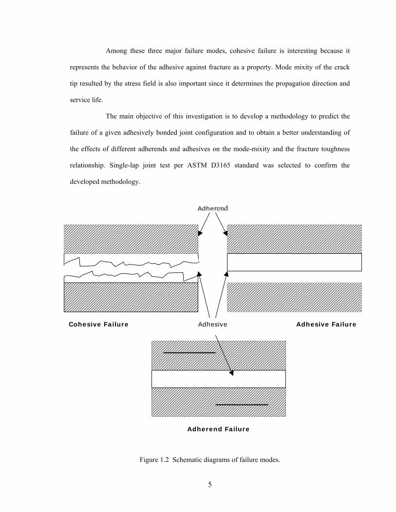
The failure mode of a joint is an important factor in the analysis, since it depicts the
weaker part of the joint and allows the designers to estimate the problem. Three major failure
modes for an adhesively bonded joint are found in literature and often used in the industry, are as
follows:
I. Cohesive Failure: where internal failure occurs in the adhesive region indicating
adhesive strength is less than the strength of the bond (Figure 1.2).
II. Adhesive Failure: where failure occurs in the interface between the adherend
and the adhesive, indicating improper surface preparation or adhesive type
(Figure 1.2).
III. Adherend Failure: where failure occurs in the adherend, especially when it is a
composite material, indicating that the interlaminar strength of the composite is
lower than the adhesive strength (Figure 1.2).
4
Among these three major failure modes, cohesive failure is interesting because it
represents the behavior of the adhesive against fracture as a property. Mode mixity of the crack
tip resulted by the stress field is also important since it determines the propagation direction and
service life.
The main objective of this investigation is to develop a methodology to predict the
failure of a given adhesively bonded joint configuration and to obtain a better understanding of
the effects of different adherends and adhesives on the mode-mixity and the fracture toughness
relationship. Single-lap joint test per ASTM D3165 standard was selected to confirm the
developed methodology.
Adhesive FailureCohesive Failure
Adherend
Adhesive
Adherend Failure
Figure 1.2 Schematic diagrams of failure modes.
5

1.3 Literature Survey
Numerous mixed-mode fracture studies have been conducted over the years,
including standardized and non-standardized test methods, analytical models, numerical and
computational studies, and the effects of manufacturing procedures on fracture toughness values.
Existing standardized tests, such as those from the American Society of Testing Materials
(ASTM) and Suppliers of Advanced Composite Materials Association (SACMA), address the
interlaminar fracture toughness of fiber-reinforced polymer matrix composites. Similar test
methods have been used to obtain fracture toughness values of adhesively bonded joints with
minor modifications to specimen configurations and test speeds due to the limited number of
standardized test methods dedicated for adhesive joints.
Most analytical models revolve around finite element analysis with different
modeling approaches because of its proven accuracy in stress analysis. The state of stress at the
crack tip is then related to the strain energy release rate, G, using traditional techniques such as
the virtual crack closure technique (VCCT) and J-integral. Modern versions of computational
stress analysis packages offer the convenience of bypassing this step and directly solving for
strain energy release rates using the above-mentioned theories. However, accuracy of these
results depends on models used in predicting the material’s behavior. It is difficult to model
adhesive behavior for its high non-linearity and vast variety.
Studies have been conducted on the effect of manufacturing variables on fracture
toughness values in adhesive joints. It has been found that manufacturing procedures, especially
in surface preparation, and environmental conditions can have a substantial effect on these
toughness values.
6
1.3.1 Theoretical Work
Weerts and Kossira [5] have studied the mixed mode fracture characterization of
adhesive joints on the basis of J-integral using double cantilever beams (DCB) and single-lap
joint (SLJ) specimens. The formulation of J-integral is used in a coarsely meshed finite element
analysis that bypasses strain singularity and inelastic behavior at the crack tip. Simple
determinations of adhesive thickness and near-tip adhesive stresses and strains of a continuum
mechanics approach allow mixed-mode characterization. Pirondi and Nicoletto [6] compared
various mixed-mode fracture criteria with experimental data using a bonded CTS specimen and a
corresponding fixture. Crack propagation in mode I and in mode II were observed to be cohesive
at the beginning but developed differently from cohesive to adhesive depending on mode mixity.
Nairn [7] emphasized the effect of residual stress consideration in mode I energy release rate
evaluation for DCB specimens and adhesives using beam theory, hence avoiding the consequence
of ignoring residual stresses, which might have resulted in measuring apparent toughness instead
of true toughness. It is also demonstrated that the error between apparent toughness and true
toughness can be large and is often larger than the correction required for crack tip rotation
effects.
Williams and Moore [8] introduced a protocol to provide guidance on the
measurement of peel strength of the laminate and to show how adhesive fracture toughness can
be determined from peel strength. Yang et al. [9] numerically studied an elastic-plastic mode II
fracture of adhesive joints. A traction-separation law was used to simulate the mode II interfacial
fracture of adhesively bonded edge notched flexure specimens loaded in three-point bending. A
shell/3D modeling technique was developed by Krueger [10], where a local solid finite element
model was used only in the immediate vicinity of the delamination front, combining the accuracy
of the full three-dimensional solution with the computational efficiency of a plate or shell finite
element model.
7
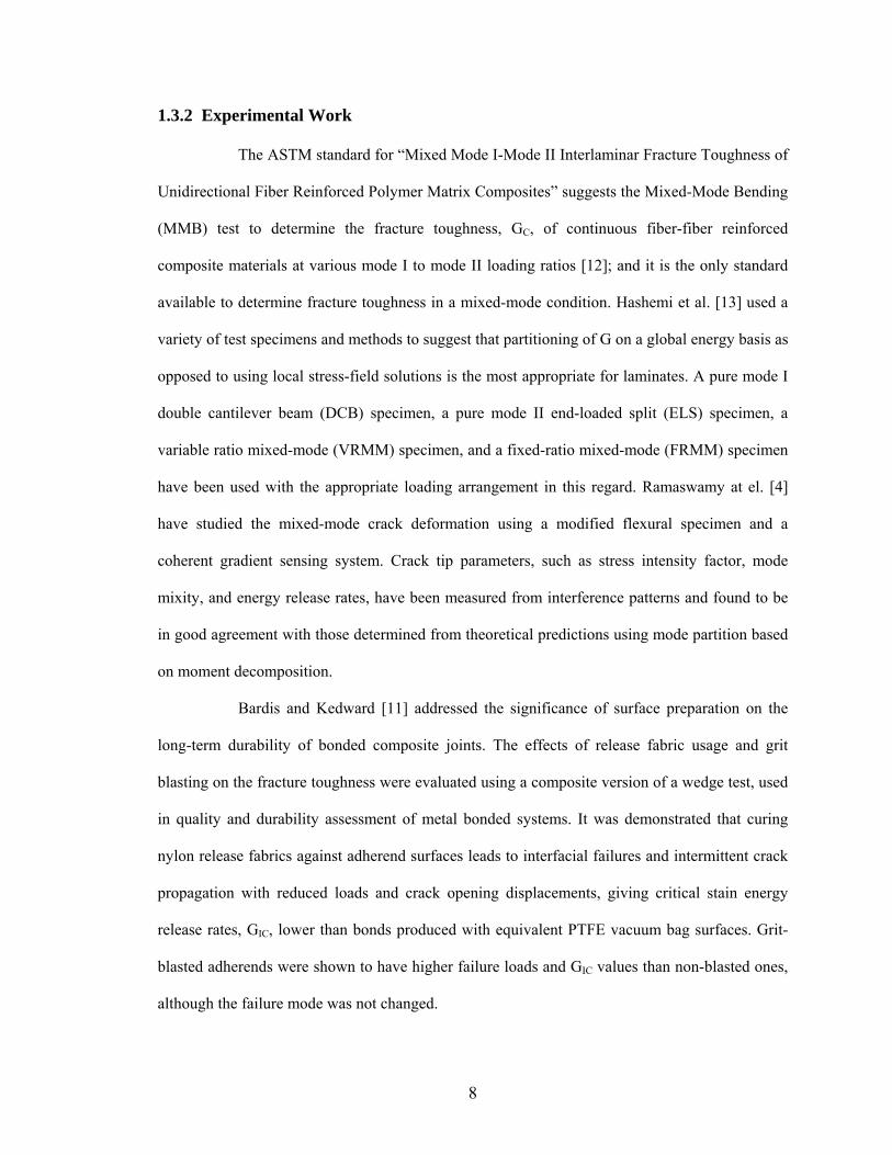
1.3.2 Experimental Work
The ASTM standard for “Mixed Mode I-Mode II Interlaminar Fracture Toughness of
Unidirectional Fiber Reinforced Polymer Matrix Composites” suggests the Mixed-Mode Bending
(MMB) test to determine the fracture toughness, GC, of continuous fiber-fiber reinforced
composite materials at various mode I to mode II loading ratios [12]; and it is the only standard
available to determine fracture toughness in a mixed-mode condition. Hashemi et al. [13] used a
variety of test specimens and methods to suggest that partitioning of G on a global energy basis as
opposed to using local stress-field solutions is the most appropriate for laminates. A pure mode I
double cantilever beam (DCB) specimen, a pure mode II end-loaded split (ELS) specimen, a
variable ratio mixed-mode (VRMM) specimen, and a fixed-ratio mixed-mode (FRMM) specimen
have been used with the appropriate loading arrangement in this regard. Ramaswamy at el. [4]
have studied the mixed-mode crack deformation using a modified flexural specimen and a
coherent gradient sensing system. Crack tip parameters, such as stress intensity factor, mode
mixity, and energy release rates, have been measured from interference patterns and found to be
in good agreement with those determined from theoretical predictions using mode partition based
on moment decomposition.
Bardis and Kedward [11] addressed the significance of surface preparation on the
long-term durability of bonded composite joints. The effects of release fabric usage and grit
blasting on the fracture toughness were evaluated using a composite version of a wedge test, used
in quality and durability assessment of metal bonded systems. It was demonstrated that curing
nylon release fabrics against adherend surfaces leads to interfacial failures and intermittent crack
propagation with reduced loads and crack opening displacements, giving critical stain energy
release rates, GIC, lower than bonds produced with equivalent PTFE vacuum bag surfaces. Grit-
blasted adherends were shown to have higher failure loads and GIC values than non-blasted ones,
although the failure mode was not changed.
8
CHAPTER 2
MIXED-MODE FRACTURE TOUGHNESS TESTING
The fracture behavior of a material for a given mode is studied by developing a
resistant curve that can be used to predict the load required for propagation. The resistance curve,
or R curve, is traditionally the strain energy release rate, G, plotted against the crack extension for
a given material. The R curve depicts a basic description of how a fracture behaves in a particular
material, since it is the energy needed for a crack to extend. Furthermore, an R curve can predict
the stable/unstable regions of the propagation by plotting the driving force against crack length
over the R curve, as shown in Figure 2.1 [14].
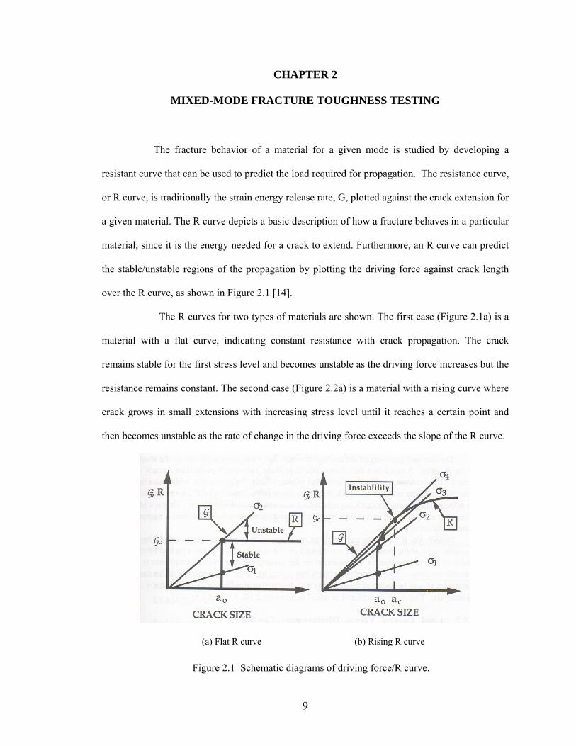
The R curves for two types of materials are shown. The first case (Figure 2.1a) is a
material with a flat curve, indicating constant resistance with crack propagation. The crack
remains stable for the first stress level and becomes unstable as the driving force increases but the
resistance remains constant. The second case (Figure 2.2a) is a material with a rising curve where
crack grows in small extensions with increasing stress level until it reaches a certain point and
then becomes unstable as the rate of change in the driving force exceeds the slope of the R curve.
e e
F
(a) Flat R curv
igure 2.1 Schematic diagrams of dri
9
(b) Rising R curv
ving force/R curve.
2.1 Background
The strain energy release rate of a certain material under a given loading condition
can be broken down into three main loading configurations and corresponding strain energy
release rate fractions as shown in Figure 1.1. This investigation is limited to mode I, mode II and
mixed-mode I and II loading configurations, hence, the total strain energy release rate consists of
mode I strain energy release rate GI and mode II strain energy release rate GII.
A mixed-mode R curve would depict the crack propagation of a material under
mixed-mode loading conditions. However, this requires a three-dimensional plot and a massive
amount of experimental test data which is beyond the scope of this study. Instead, a mode-mixity
fracture toughness curve is considered in this investigation, addressing only the fracture initiation
of a given crack length. Mode mixity has been noted in the literature as a percentage of the strain
energy release rate value corresponding to the mode II portion of the load over the total strain
energy release rate, GT which is used in this study as shown in Equation 2.1. Therefore 0% mode-
mixity corresponds to the pure mode I and 100% mode-mixity corresponds to pure mode II
loading condition.
T
II
III
IIII G
GGG
GG =+
=% (2.1)
In order to develop a mixed-mode fracture toughness curve for a particular material,
the fracture toughness or critical strain energy release rate, GC, needs to be determined at each
mode-mixity point, ranging from pure mode I or 0% mode-mixity, to pure mode II, or 100%
mode-mixity. It should be noted that the strain energy release rate that is necessary to propagate a
crack is referred to as the critical strain energy release rate or fracture toughness, hence, used in
plotting the mode-mixity fracture toughness curve. Numerous techniques are available to
determine fracture toughness for a given mode. ASTM and SACMA standardized test methods
are used in this investigation.
10
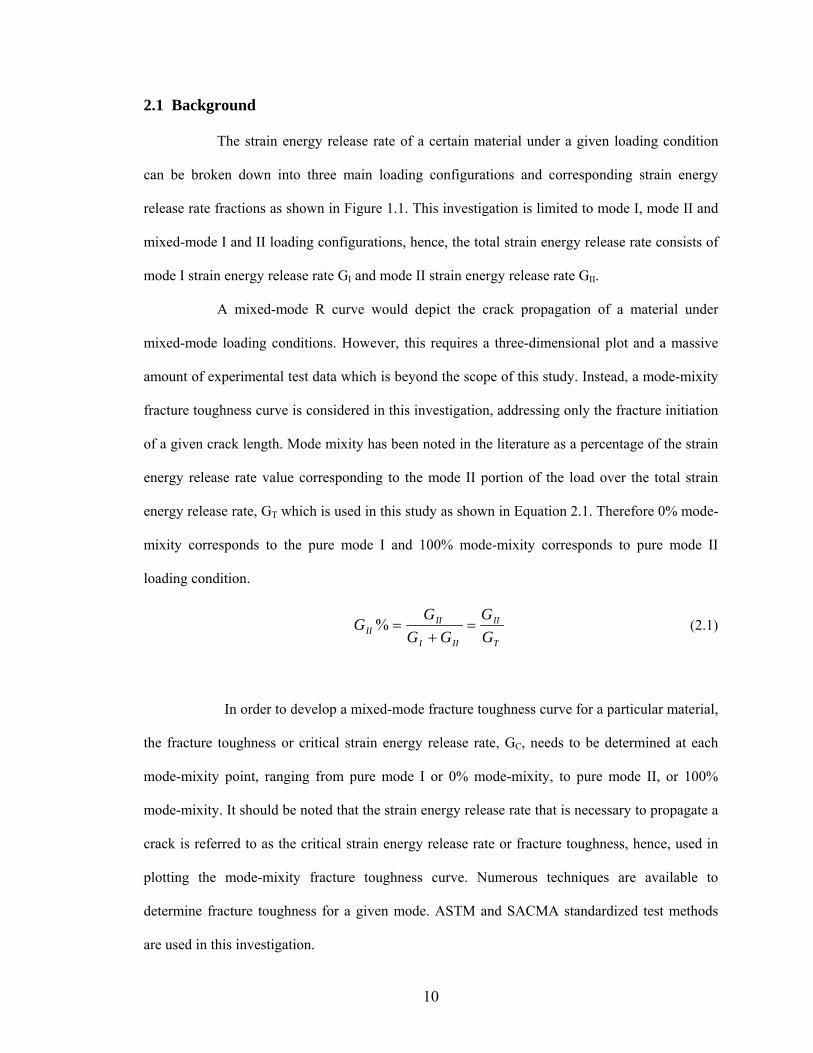
2.1.1 Mode I
ASTM recommends D5528 standard for mode I interlaminar fracture toughness.
Although this test method is meant for interlaminar fracture toughness of unidirectional
composite laminates, it can also be used for adhesive-bonded joints [15]. Specimen configuration
is similar to what the standard suggests. The double cantilever beam (DCB) with piano hinges, as
shown in Figure 2.2, consists of two adherends bonded with adhesive.
Piano Hinges Adherend
Adhesive LayerInitial Crack P
P
Figure 2.2a Schematic diagram of mode I DCB specimen (side view).
The mode I critical strain energy release rate, GIC, was determined using the modified
beam theory (MBT), which accounts for rotation at the delamination front, as recommended in
ASTM D5528 standard. The final data reduction formula is shown in Equation 2.2. An initial
crack length of two inches is recommended.
)(23
∆+=
abPGI
δ (2.2)
where:
P = Load δ = Load point displacement b = Specimen width a = Crack length ∆ = Correction factor for rotation
11
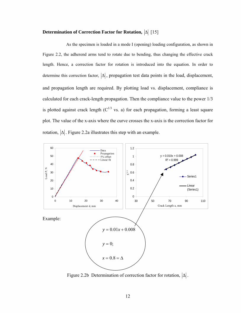
Determination of Correction Factor for Rotation, ∆ [15]
As the specimen is loaded in a mode I (opening) loading configuration, as shown in
Figure 2.2, the adherend arms tend to rotate due to bending, thus changing the effective crack
length. Hence, a correction factor for rotation is introduced into the equation. In order to
determine this correction factor, ∆ , propagation test data points in the load, displacement,
and propagation length are required. By plotting load vs. displacement, compliance is
calculated for each crack-length propagation. Then the compliance value to the power 1/3
is plotted against crack length (C1/3 vs. a) for each propagation, forming a least square
plot. The value of the x-axis where the curve crosses the x-axis is the correction factor for
rotation, ∆ . Figure 2.2a illustrates this step with an example.
0
10
20
30
40
50
60
0 10 20 30 40
Displacement d, mm
Loa
d P,
N
DataPropagation5% offsetLinear fit
y = 0.010x + 0.008R2 = 0.999
0
0.2
0.4
0.6
0.8
1
1.2
30 50 70 90 110Crack Length a, mm
C1/
3
Series1
Linear(Series1)
Example:
∆==
=
+=
8.0
;0
008.001.0
x
y
xy
Figure 2.2b Determination of correction factor for rotation, ∆ .
12
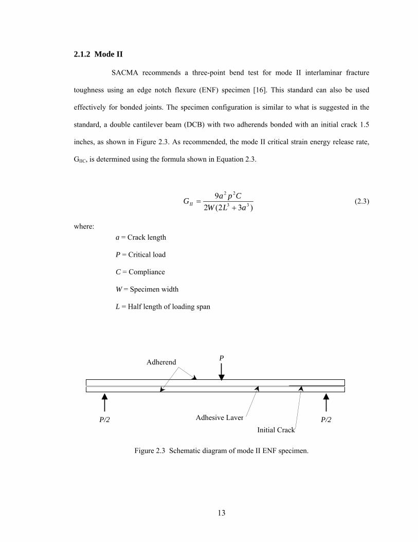
2.1.2 Mode II
SACMA recommends a three-point bend test for mode II interlaminar fracture
toughness using an edge notch flexure (ENF) specimen [16]. This standard can also be used
effectively for bonded joints. The specimen configuration is similar to what is suggested in the
standard, a double cantilever beam (DCB) with two adherends bonded with an initial crack 1.5
inches, as shown in Figure 2.3. As recommended, the mode II critical strain energy release rate,
GIIC, is determined using the formula shown in Equation 2.3.
)32(29
33
22
aLWCpaGII +
= (2.3)
where:
P/2
a = Crack length P = Critical load C = Compliance W = Specimen width L = Half length of loading span
Initial Crack
Adherend
Adhesive Layer P/2
P
Figure 2.3 Schematic diagram of mode II ENF specimen.
13
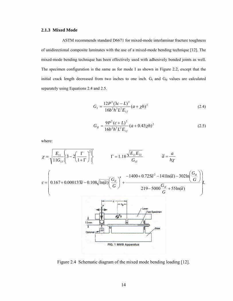
2.1.3 Mixed Mode
ASTM recommends standard D6671 for mixed-mode interlaminar fracture toughness
of unidirectional composite laminates with the use of a mixed-mode bending technique [12]. The
mixed-mode bending technique has been effectively used with adhesively bonded joints as well.
The specimen configuration is the same as for mode I as shown in Figure 2.2, except that the
initial crack length decreased from two inches to one inch. GI and GII values are calculated
separately using Equations 2.4 and 2.5.
2
1232
22
)(16
)3(12 haELhbLcPG
fI χ+
−= (2.4)
2
1232
22
)43.0(16
)(9 haELhbLcPG
fII χ+
+= (2.5)
where:
⎪⎭
⎪⎬⎫
⎪⎩
⎪⎨⎧
⎟⎠⎞
⎜⎝⎛
Γ+Γ
−=2
13
11
123
11GE
χ 13
221118.1G
EE=Γ
χhaa =~
La
GG
GG
aa
GG
aacII
II
II
⎟⎟⎟⎟⎟
⎠
⎞
⎜⎜⎜⎜⎜
⎝
⎛
+−
⎟⎠⎞
⎜⎝⎛−−+−
+⎟⎠⎞
⎜⎝⎛−+=
)~ln(555000219
ln302)~ln(141~725.01400)~ln(108.0~000137.0167.0
24
Figure 2.4 Schematic diagram of the mixed mode bending loading [12].
14
2.2 Panel Fabrication and Bonding
This section addresses panel fabrication and bonding, required to fabricate test
specimens necessary to generate mode-mixity fracture toughness curves. Panel fabrication
involves material selection, adhesive selection, surface preparation, and bonding procedures
including cure cycles. This may be the most important step of the entire investigation, since it
directly affects the test results. Material and adhesive selection may be approached with a sense
of an actual adhesive joint that is useful to the industry. Surface preparation effects on adhesive
joint behavior have been investigated previously especially on fracture toughness, and mentioned
in the literature survey section [11].
The bonding procedure may change with the type of adhesive used according to the
manufacturer recommendations. The cure cycle used for bonding may affect the toughness of the
joint. A room temperature-cured adhesive joint may not behave the same as an elevated
temperature-cured joint. With so many techniques and procedures available, it is important to be
consistent with the fabrication process so that the results obtained are valid for comparison. Some
of the key factors in the panel fabrication and bonding process that could affect the final results
are listed here:
• Adherend properties (material, layup, thickness, etc.)
• Adherend preparation (layup process, cure cycle, surface roughness, etc.)
• Adhesive properties (adhesive type, bulk adhesive properties, etc.)
• Adhesive preparation (accuracy of mixing ratios, environmental conditions, etc.)
• Bonding method (bond line thickness control, environmental conditions, etc)
• Cure cycle (curing technique, accuracy of apparatus, environmental conditions, etc.)
15
2.2.1 Material Selection and Cure-Cycle
Materials were selected based on the most common single-lap shear test specimens
used in the industry. Although it is most common to use aluminum adherends as single-lap shear
test specimens to simulate adhesive-bonded joints in shear, the current trend toward composite-
adhesive joints led this investigation to select carbon fiber and glass fiber materials. However,
anodized aluminum 2024-T3 was also used with the composite adherends to fabricate specimens,
in order to understand the effect of adherend material. Resin pre-impregnated materials, better
known as prepregs, were used to make adherend panels because of their wide use, availability,
and convenience. Three types of adherends were used in this investigation: one with a carbon
fiber unitape and fabric combination, a glass fabric, and aluminum. Basic information about the
prepreg materials used in adherends is listed in Table 2.1.
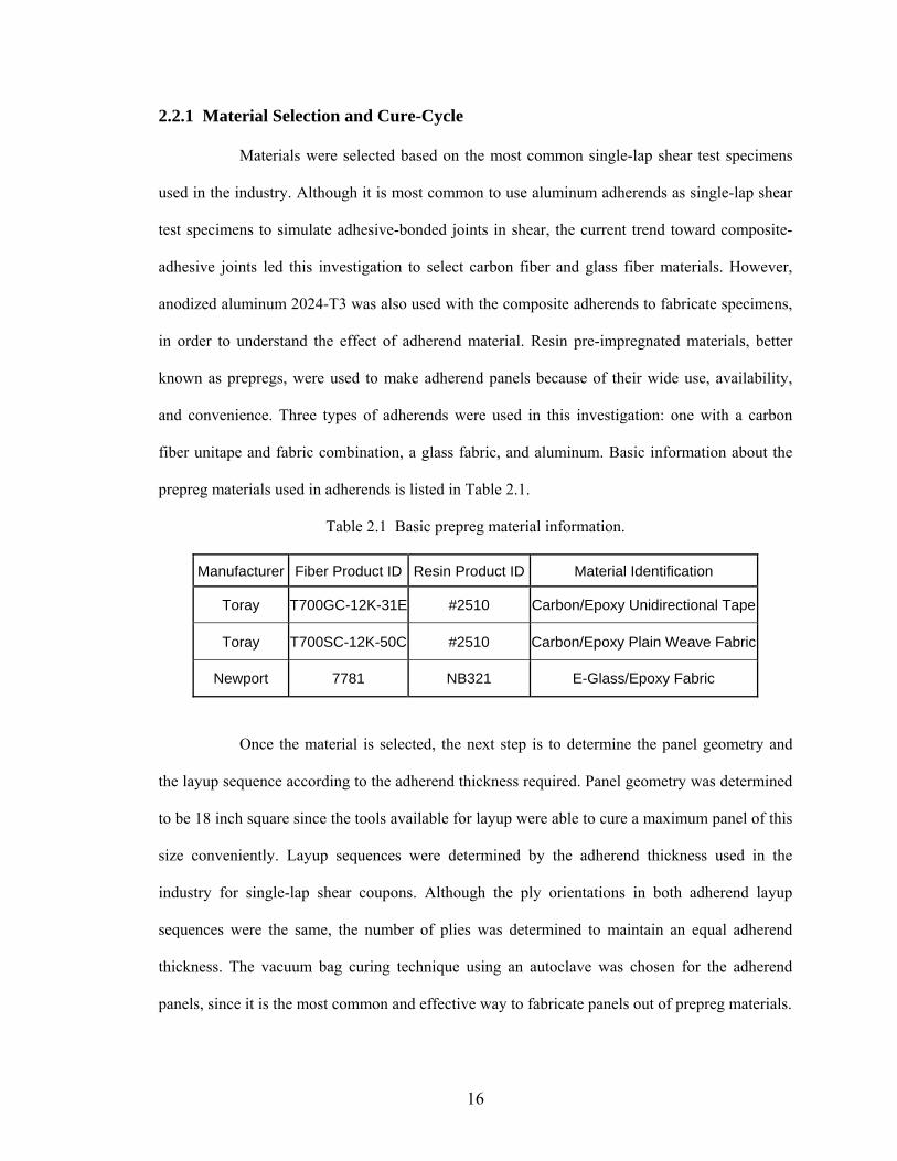
Table 2.1 Basic prepreg material information.
Manufacturer Fiber Product ID Resin Product ID Material Identification
Toray T700GC-12K-31E #2510 Carbon/Epoxy Unidirectional Tape
Toray T700SC-12K-50C #2510 Carbon/Epoxy Plain Weave Fabric
Newport 7781 NB321 E-Glass/Epoxy Fabric
Once the material is selected, the next step is to determine the panel geometry and
the layup sequence according to the adherend thickness required. Panel geometry was determined
to be 18 inch square since the tools available for layup were able to cure a maximum panel of this
size conveniently. Layup sequences were determined by the adherend thickness used in the
industry for single-lap shear coupons. Although the ply orientations in both adherend layup
sequences were the same, the number of plies was determined to maintain an equal adherend
thickness. The vacuum bag curing technique using an autoclave was chosen for the adherend
panels, since it is the most common and effective way to fabricate panels out of prepreg materials.
16
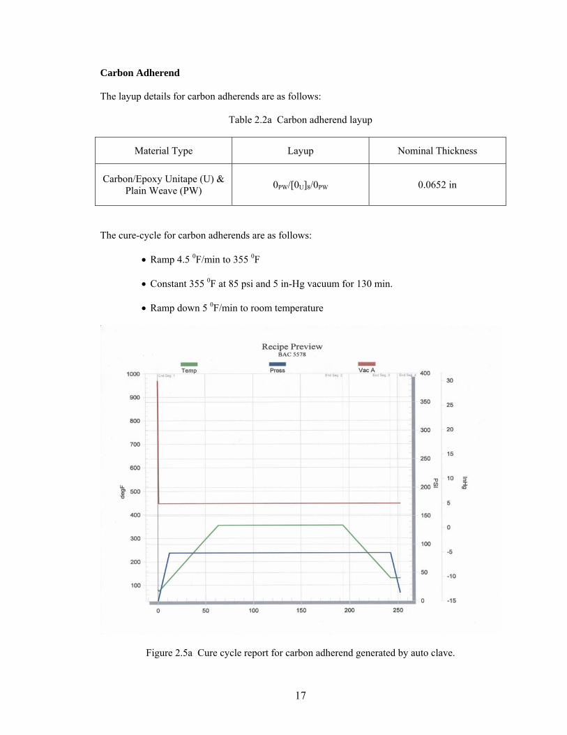
Carbon Adherend
The layup details for carbon adherends are as follows:
Table 2.2a Carbon adherend layup
Material Type Layup Nominal Thickness
Carbon/Epoxy Unitape (U) & Plain Weave (PW) 0PW/[0U]8/0PW 0.0652 in
The cure-cycle for carbon adherends are as follows:
• Ramp 4.5 0F/min to 355 0F
• Constant 355 0F at 85 psi and 5 in-Hg vacuum for 130 min.
• Ramp down 5 0F/min to room temperature
Figure 2.5a Cure cycle report for carbon adherend generated by auto clave.
17
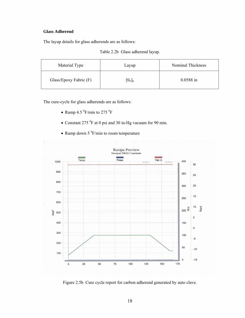
Glass Adherend
The layup details for glass adherends are as follows:
Table 2.2b Glass adherend layup.
Material Type Layup Nominal Thickness
Glass/Epoxy Fabric (F) [0F]6 0.0588 in
The cure-cycle for glass adherends are as follows:
• Ramp 4.5 0F/min to 275 0F
• Constant 275 0F at 0 psi and 30 in-Hg vacuum for 90 min.
• Ramp down 5 0F/min to room temperature
Figure 2.5b Cure cycle report for carbon adherend generated by auto clave.
18
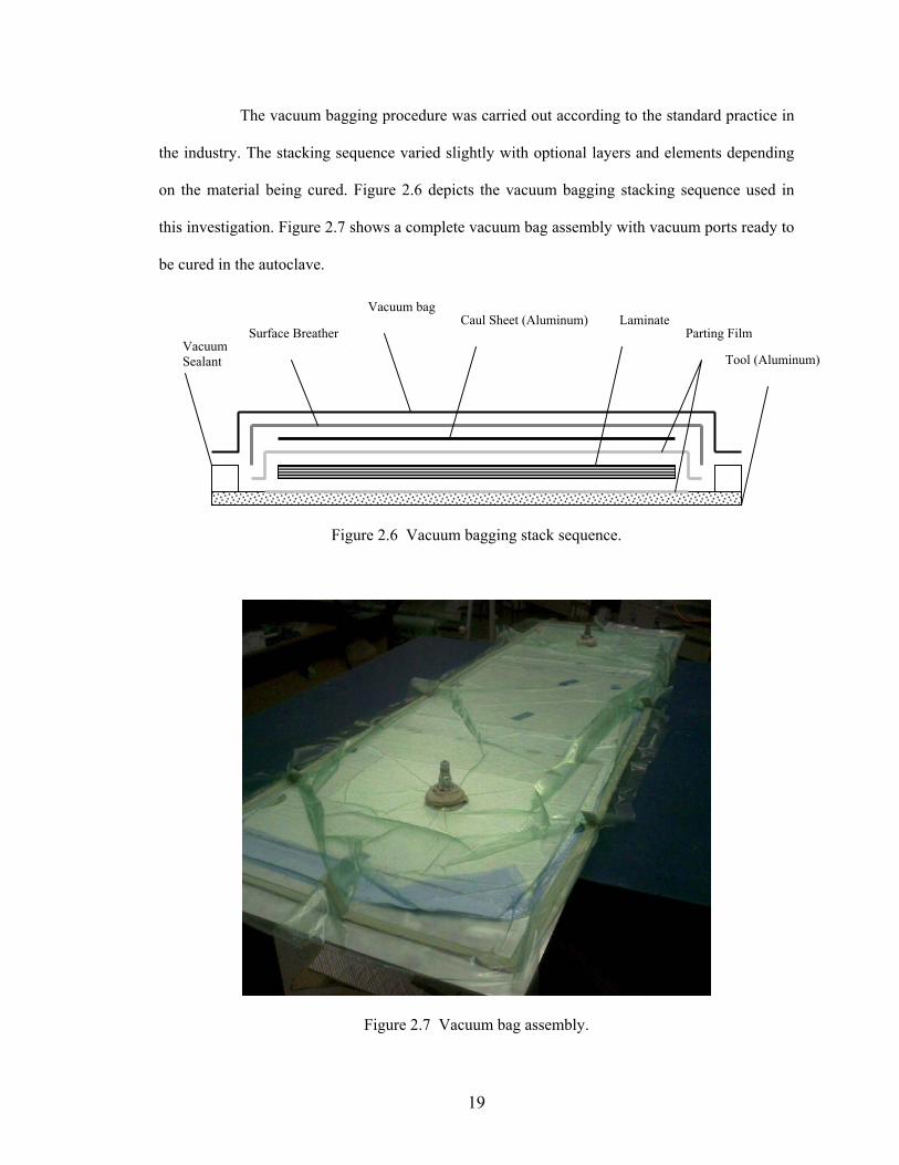
The vacuum bagging procedure was carried out according to the standard practice in
the industry. The stacking sequence varied slightly with optional layers and elements depending
on the material being cured. Figure 2.6 depicts the vacuum bagging stacking sequence used in
this investigation. Figure 2.7 shows a complete vacuum bag assembly with vacuum ports ready to
be cured in the autoclave.
VacuumSea
lant
Vacuum bagLaminate
Parting Film
Tool (Aluminum)
Surface Breather Caul Sheet (Aluminum)
Figure 2.6 Vacuum bagging stack sequence.
Figure 2.7 Vacuum bag assembly.
19
2.2.2 Surface Preparation
Surface preparation of the panels to be bonded is an important step since it directly
affects the strength of the adhesive bond that affects the failure mode. By preparing surface
correctly, joint strength can be maintained to its full potential, resulting in long-term structural
integrity. Incorrect surface preparation could lead to adhesive bond failure and unpredictable
failure. The primary role of surface preparation is to remove surface contaminants, increase the
bonding surface area, and improve surface roughness.
In this investigation, surface preparation was performed in accordance with the
industry, adhering to the adhesive manufacturer recommendations. Surface roughness is a key
factor in surface preparation. Sanding the surface to be bonded is the regular approach to
increasing its roughness. However, hand sanding has a tendency to leave an uneven roughness
across the panel surface. Sand blaster machines are often used because of their ability to sand a
surface fairly even and the option to control pressure, thus allowing the user to achieve the
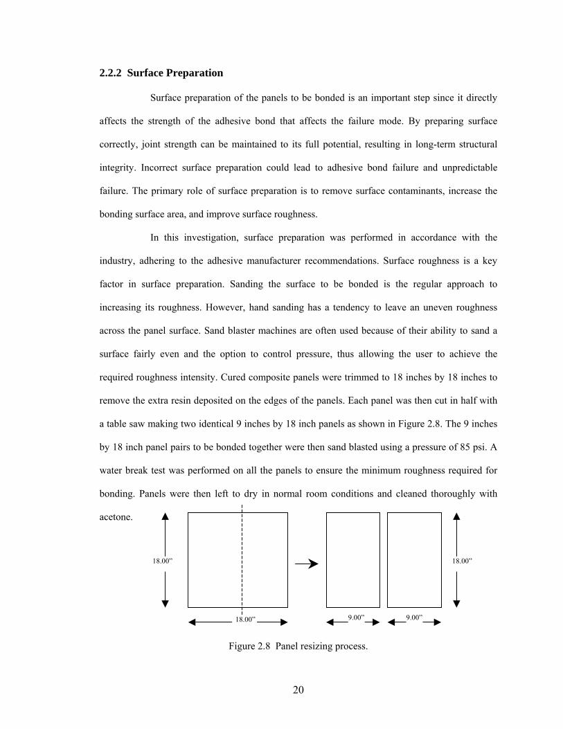
required roughness intensity. Cured composite panels were trimmed to 18 inches by 18 inches to
remove the extra resin deposited on the edges of the panels. Each panel was then cut in half with
a table saw making two identical 9 inches by 18 inch panels as shown in Figure 2.8. The 9 inches
by 18 inch panel pairs to be bonded together were then sand blasted using a pressure of 85 psi. A
water break test was performed on all the panels to ensure the minimum roughness required for
bonding. Panels were then left to dry in normal room conditions and cleaned thoroughly with
acetone.
18.00” 9.00” 9.00”
18.00” 18.00”
Figure 2.8 Panel resizing process.
20
2.2.3 Adhesive Selection and Bonding Method
Adhesive selection was based on the industry’s use of adhesives on single-lap shear
testing since it allows one to utilize the findings of this investigation to benefit the industry itself.
Paste adhesive EA 9394 manufactured by Hysol is a widely used adhesive in the aviation
industry, known for its proven high strengths in high-temperatures environments as well as low-
temperature environments and long pot life, making it convenient to work with. Film adhesives
have long being used in the industry for their convenience, less wastage, and high strength
properties. The film adhesive EA 9628 manufactured by Hysol is a widely used film adhesive in
the industry. Table 2.3 summarizes the features of both adhesives.
Table 2.3 Summary of features of selected adhesives.
EA 9394 (Paste) EA 9628 (Film)
Room Temperature Cure Good Toughness
Good Gap Filling Capabilities 235-250F/113-121C Cure
350F/177C Performance Bonds Many Materials
Potting Material Excellent Durability
Room Temperature Storage Film Adhesive
Long Pot Life Less waste
Low Toxity
The above-mentioned adhesive types along with carbon and glass adherends
introduced in the previous section were chosen to generate response curves. After narrowing
down the adhesive and adherend types, the next step was to bond panels with proper care and
cure then in appropriate temperature and pressure conditions. The two most important aspects of
the bonding process are to maintain a constant bond-line thickness and a proper pre-crack
simulation technique.
21

It was determined that a bond-line thickness of 0.015 inch was satisfactory to
compare the results since the industrial adhesive joint bond-line thickness was within that range
as were most thick single-lap shear coupons tested. Many techniques are being followed to
maintain a constant bond-line thickness in test coupons. Glass micro-beads embedded in
adhesives, metal spacers, and bladder pressure techniques are some of the popular techniques.
Since the type of adhesives selected for this investigation do not contain micro beads, metal
spacers were used to maintain the required bond-line thickness. After a few bonding trials, a
spacer with a thickness of 0.01 inch was chosen for this investigation. Although the material of
the spacers does not have an effect on the results, it should be noted that the spacers were made
from brass. In order to make the panel bonding area uniform through-out, a bladder press was
used because of its ability to control the pressure applied on the bonding panels.
After a number of trials using various methods to simulate an initial crack, it was
determined that applying a few layers of utility tape to both sides of the initial crack area worked
best. However, pre-cracking is important for specimens that are fabricated using this method in
order to simulate a realistic cohesive crack. The number of utility tape layers should compliment
the overall bond-line thickness of the specimen. Since the thickness of tape used was measured to
be 0.0025 inch, it was determined that four layers of utility with two layers for each surface were
necessary.
All the panels were bonded using the same technique in order to maintain the process
consistency. Panels bonded with EA 9394 paste adhesive were cured at room temperature for five
days, as recommended by the manufacturer, while EA 9628 film adhesive bonded panels were
bonded in an oven at 250 0F. All panels were bonded using the same bladder press with a constant
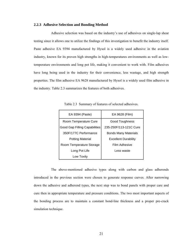
pressure of 20 psi. Figures 2.9a though 2.9c show the panels bonded with spacers and adhesives,
summarizing the bonding process mentioned above.
22
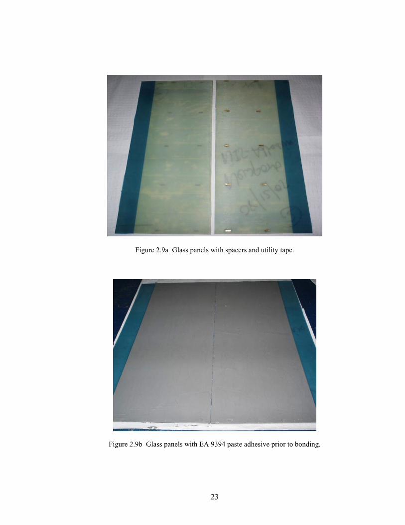
Figure 2.9a Glass panels with spacers and utility tape.
Figure 2.9b Glass panels with EA 9394 paste adhesive prior to bonding.
23
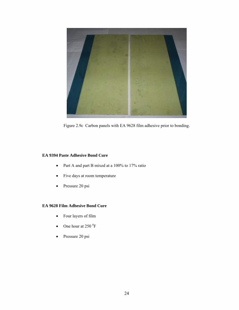
Figure 2.9c Carbon panels with EA 9628 film adhesive prior to bonding.
EA 9394 Paste Adhesive Bond Cure
• Part A and part B mixed at a 100% to 17% ratio
• Five days at room temperature
• Pressure 20 psi
EA 9628 Film Adhesive Bond Cure
• Four layers of film
• One hour at 250 0F
• Pressure 20 psi
24
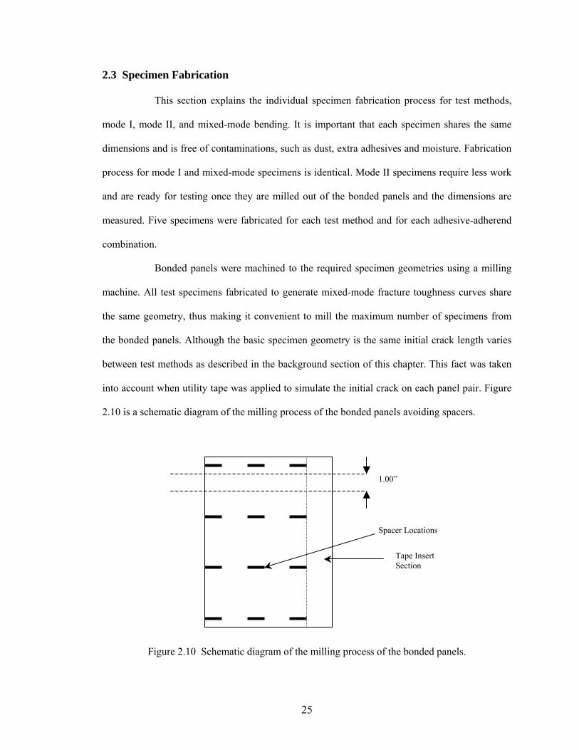
2.3 Specimen Fabrication
This section explains the individual specimen fabrication process for test methods,
mode I, mode II, and mixed-mode bending. It is important that each specimen shares the same
dimensions and is free of contaminations, such as dust, extra adhesives and moisture. Fabrication
process for mode I and mixed-mode specimens is identical. Mode II specimens require less work
and are ready for testing once they are milled out of the bonded panels and the dimensions are
measured. Five specimens were fabricated for each test method and for each adhesive-adherend
combination.
Bonded panels were machined to the required specimen geometries using a milling
machine. All test specimens fabricated to generate mixed-mode fracture toughness curves share
the same geometry, thus making it convenient to mill the maximum number of specimens from
the bonded panels. Although the basic specimen geometry is the same initial crack length varies
between test methods as described in the background section of this chapter. This fact was taken
into account when utility tape was applied to simulate the initial crack on each panel pair. Figure
2.10 is a schematic diagram of the milling process of the bonded panels avoiding spacers.
Tape Insert Section
Spacer Locations
1.00”
Figure 2.10 Schematic diagram of the milling process of the bonded panels.
25
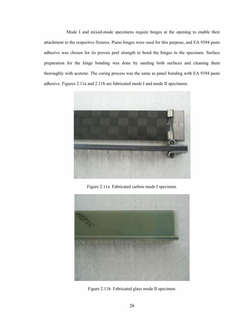
Mode I and mixed-mode specimens require hinges at the opening to enable their
attachment to the respective fixtures. Piano hinges were used for this purpose, and EA 9394 paste
adhesive was chosen for its proven peel strength to bond the hinges to the specimen. Surface
preparation for the hinge bonding was done by sanding both surfaces and cleaning them
thoroughly with acetone. The curing process was the same as panel bonding with EA 9394 paste
adhesive. Figures 2.11a and 2.11b are fabricated mode I and mode II specimens.
Figure 2.11a Fabricated carbon mode I specimen.
Figure 2.11b Fabricated glass mode II specimen.
26
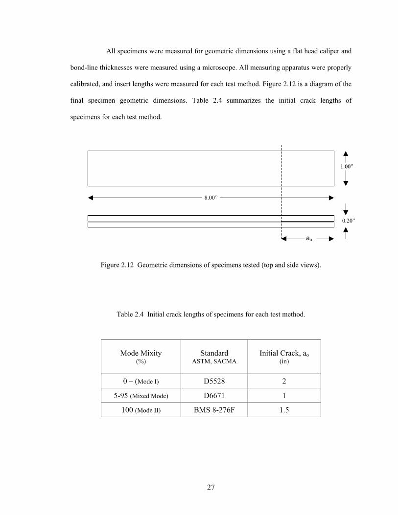
All specimens were measured for geometric dimensions using a flat head caliper and
bond-line thicknesses were measured using a microscope. All measuring apparatus were properly
calibrated, and insert lengths were measured for each test method. Figure 2.12 is a diagram of the
final specimen geometric dimensions. Table 2.4 summarizes the initial crack lengths of
specimens for each test method.
ao
0.20”
8.00”
1.00”
Figure 2.12 Geometric dimensions of specimens tested (top and side views).
Table 2.4 Initial crack lengths of specimens for each test method.
Mode Mixity (%)
Standard ASTM, SACMA
Initial Crack, ao (in)
0 – (Mode I) D5528 2
5-95 (Mixed Mode) D6671 1
100 (Mode II) BMS 8-276F 1.5
27
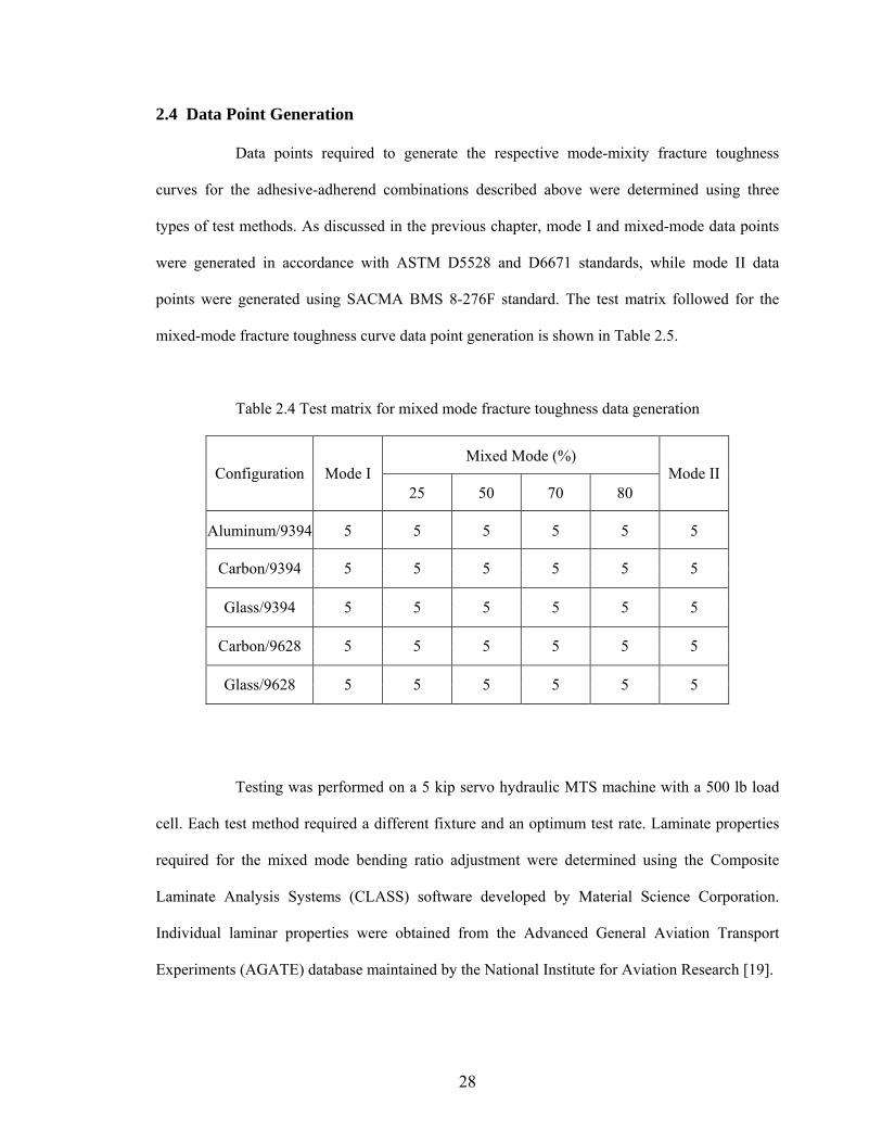
2.4 Data Point Generation
Data points required to generate the respective mode-mixity fracture toughness
curves for the adhesive-adherend combinations described above were determined using three
types of test methods. As discussed in the previous chapter, mode I and mixed-mode data points
were generated in accordance with ASTM D5528 and D6671 standards, while mode II data
points were generated using SACMA BMS 8-276F standard. The test matrix followed for the
mixed-mode fracture toughness curve data point generation is shown in Table 2.5.
Table 2.4 Test matrix for mixed mode fracture toughness data generation
Mixed Mode (%) Configuration Mode I
25 50 70 80 Mode II
Aluminum/9394 5 5 5 5 5 5
Carbon/9394 5 5 5 5 5 5
Glass/9394 5 5 5 5 5 5
Carbon/9628 5 5 5 5 5 5
Glass/9628 5 5 5 5 5 5
Testing was performed on a 5 kip servo hydraulic MTS machine with a 500 lb load
cell. Each test method required a different fixture and an optimum test rate. Laminate properties
required for the mixed mode bending ratio adjustment were determined using the Composite
Laminate Analysis Systems (CLASS) software developed by Material Science Corporation.
Individual laminar properties were obtained from the Advanced General Aviation Transport
Experiments (AGATE) database maintained by the National Institute for Aviation Research [19].
28
2.4.1 Testing Procedure
Mode I
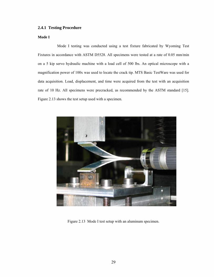
Mode I testing was conducted using a test fixture fabricated by Wyoming Test
Fixtures in accordance with ASTM D5528. All specimens were tested at a rate of 0.05 mm/min
on a 5 kip servo hydraulic machine with a load cell of 500 lbs. An optical microscope with a
magnification power of 100x was used to locate the crack tip. MTS Basic TestWare was used for
data acquisition. Load, displacement, and time were acquired from the test with an acquisition
rate of 10 Hz. All specimens were precracked, as recommended by the ASTM standard [15].
Figure 2.13 shows the test setup used with a specimen.
Figure 2.13 Mode I test setup with an aluminum specimen.
29
Mode II
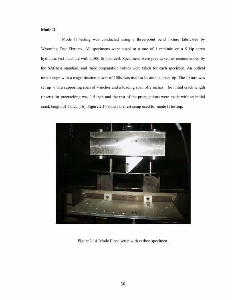
Mode II testing was conducted using a three-point bend fixture fabricated by
Wyoming Test Fixtures. All specimens were tested at a rate of 1 mm/min on a 5 kip servo
hydraulic test machine with a 500 lb load cell. Specimens were precracked as recommended by
the SACMA standard, and three propagation values were taken for each specimen. An optical
microscope with a magnification power of 100x was used to locate the crack tip. The fixture was
set up with a supporting span of 4 inches and a loading span of 2 inches. The initial crack length
(insert) for precracking was 1.5 inch and the rest of the propagations were made with an initial
crack length of 1 inch [16]. Figure 2.14 shows the test setup used for mode II testing.
Figure 2.14 Mode II test setup with carbon specimen.
30

Mixed-Mode
Mixed-mode testing for the desired ratios was conducted using a mixed-mode
bending fixture fabricated by Wyoming Test Fixtures in accordance with ASTM D6671 on a 5
kip servo hydraulic test machine with a 500 lb load cell. Figure 2.15 depicts the test setup used in
this investigation with an optical microscope with a magnification power of 100x to locate the
crack tip. The data acquisition procedure was the same as for mode I and mode II tests. The lever
length was adjusted to obtain the desired mix ratio in accordance with the standard using the
laminate properties of each adherend. It was determined to use one lever length for each mode-
mixity ratio on all specimens since the calculated lever lengths only varied one 100th of an inch.
Table 2.5 shows the lever lengths used for each mode mixity.
Table 2.5 Lever lengths used for mode mixity ratios.
Mixity (%) 25 50 70 80
c (in) 3 1.7 1.25 1.1
Figure 2.15 Mixed-mode test setup with a glass specimen.
31
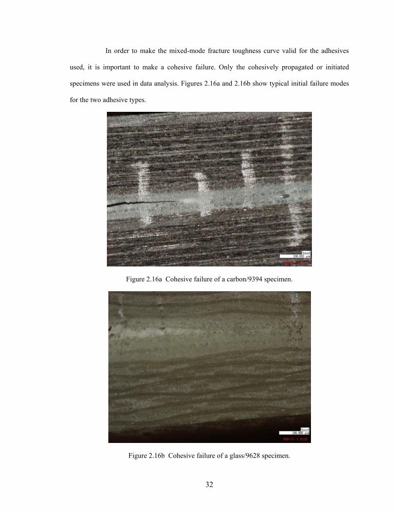
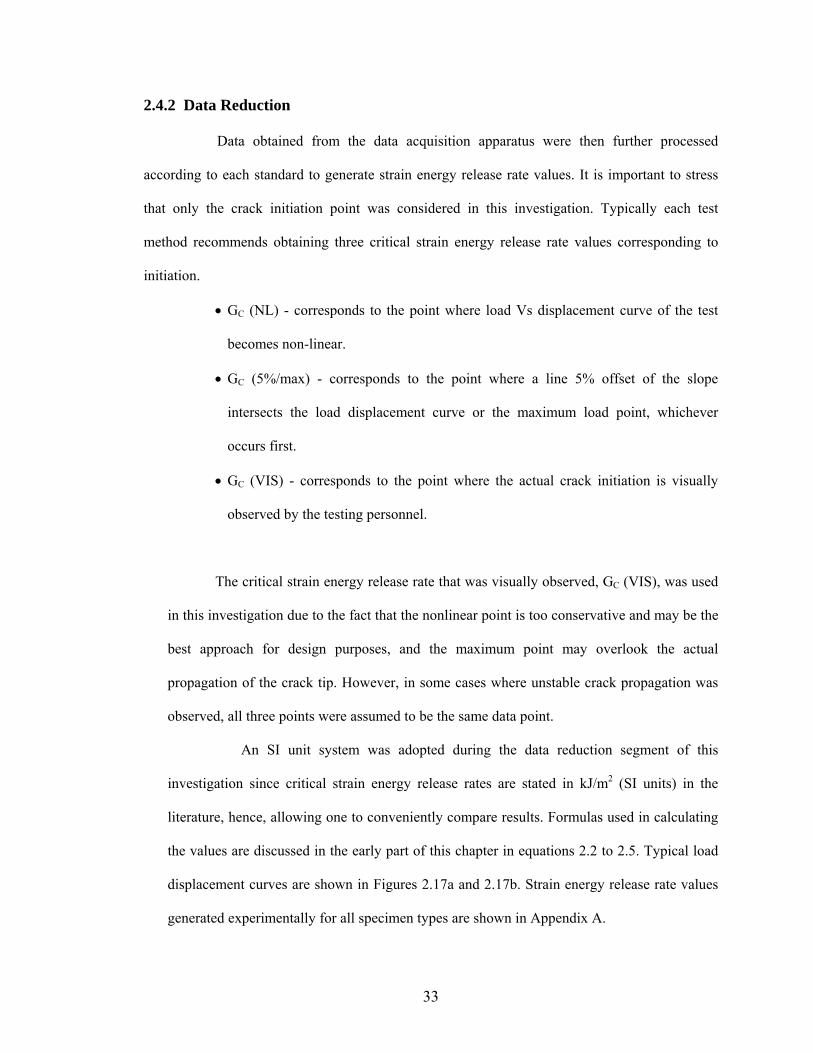
In order to make the mixed-mode fracture toughness curve valid for the adhesives
used, it is important to make a cohesive failure. Only the cohesively propagated or initiated
specimens were used in data analysis. Figures 2.16a and 2.16b show typical initial failure modes
for the two adhesive types.
Figure 2.16a Cohesive failure of a carbon/9394 specimen.
Figure 2.16b Cohesive failure of a glass/9628 specimen.
32
2.4.2 Data Reduction
Data obtained from the data acquisition apparatus were then further processed
according to each standard to generate strain energy release rate values. It is important to stress
that only the crack initiation point was considered in this investigation. Typically each test
method recommends obtaining three critical strain energy release rate values corresponding to
initiation.
• GC (NL) - corresponds to the point where load Vs displacement curve of the test
becomes non-linear.
• GC (5%/max) - corresponds to the point where a line 5% offset of the slope
intersects the load displacement curve or the maximum load point, whichever
occurs first.
• GC (VIS) - corresponds to the point where the actual crack initiation is visually
observed by the testing personnel.
The critical strain energy release rate that was visually observed, GC (VIS), was used
in this investigation due to the fact that the nonlinear point is too conservative and may be the
best approach for design purposes, and the maximum point may overlook the actual
propagation of the crack tip. However, in some cases where unstable crack propagation was
observed, all three points were assumed to be the same data point.
An SI unit system was adopted during the data reduction segment of this
investigation since critical strain energy release rates are stated in kJ/m2 (SI units) in the
literature, hence, allowing one to conveniently compare results. Formulas used in calculating
the values are discussed in the early part of this chapter in equations 2.2 to 2.5. Typical load
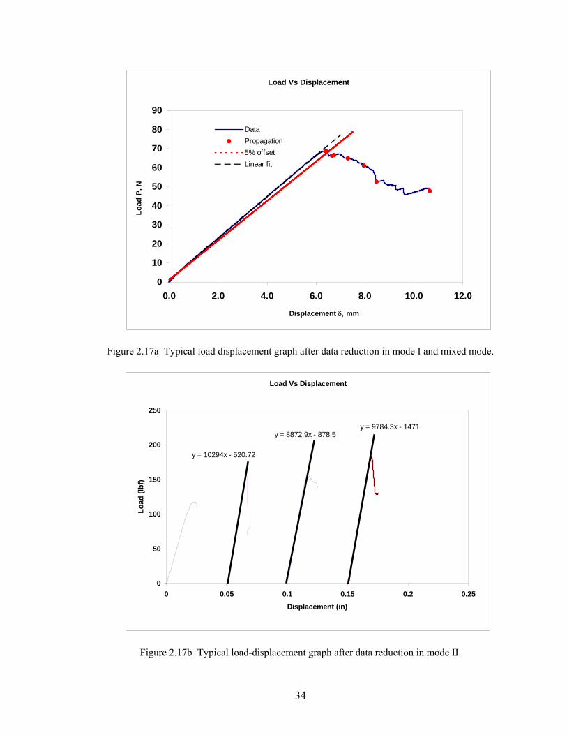
displacement curves are shown in Figures 2.17a and 2.17b. Strain energy release rate values
generated experimentally for all specimen types are shown in Appendix A.
33
Load Vs Displacement
0
10
20
30
40
50
60
70
80
90
0.0 2.0 4.0 6.0 8.0 10.0 12.0
Displacement δ, mm
Load
P, N
DataPropagation5% offsetLinear fit
Figure 2.17a Typical load displacement graph after data reduction in mode I and mixed mode.
Load Vs Displacement
y = 10294x - 520.72
y = 8872.9x - 878.5y = 9784.3x - 1471
0
50
100
150
200
250
0 0.05 0.1 0.15 0.2 0.25Displacement (in)
Load
(lbf
)
Figure 2.17b Typical load-displacement graph after data reduction in mode II.
34

CHAPTER 3
SINGLE-LAP JOINT TESTING
The single-lap joint test method recommended by ASTM D3165 is intended to
determine the shear strength of adhesively bonded joints. Although this test method is designed
for metal adherend joints, the standard document states that it may also be used with other
adherends such as composites [3]. Industry has been using this method successfully to determine
shear properties of adhesively bonded composite joints. In this investigation, single-lap joint data
is used to confirm the methodology developed to predict the failure load or stress of a given
adhesive joint. The test specimen configuration recommended by ASTM 3165 involves some
machining issues especially with composite adherends that affect the overall test results; hence, it
was determined to use a slightly different configuration to eliminate the imperfections of the
simulated adhesive joint.
Adherend and adhesive selection was the same as discussed in previous chapters
since the mode-mixity fracture toughness curves generated were intended as a tool to predict the
failure load of the single-lap joint. It is important to maintain the same bond-line thickness and
other physical characteristic in the single-lap shear specimens as the specimens tested for fracture
toughness in the previous chapter in order to minimize the dependent variables. Bonding
procedures were the same as those used on previous specimens since the adhesive and adherend
types were the same.
The test method and apparatus used for single-lap shear strength determinations were
the same as the ASTM standard recommendations including data reduction procedures. Failure
modes of the test specimens were closely examined to ensure the similarities to the fracture
toughness specimen failure modes.
35
3.1 Background
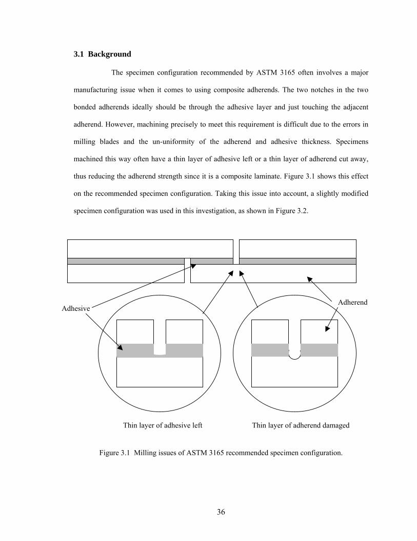
The specimen configuration recommended by ASTM 3165 often involves a major
manufacturing issue when it comes to using composite adherends. The two notches in the two
bonded adherends ideally should be through the adhesive layer and just touching the adjacent
adherend. However, machining precisely to meet this requirement is difficult due to the errors in
milling blades and the un-uniformity of the adherend and adhesive thickness. Specimens
machined this way often have a thin layer of adhesive left or a thin layer of adherend cut away,
thus reducing the adherend strength since it is a composite laminate. Figure 3.1 shows this effect
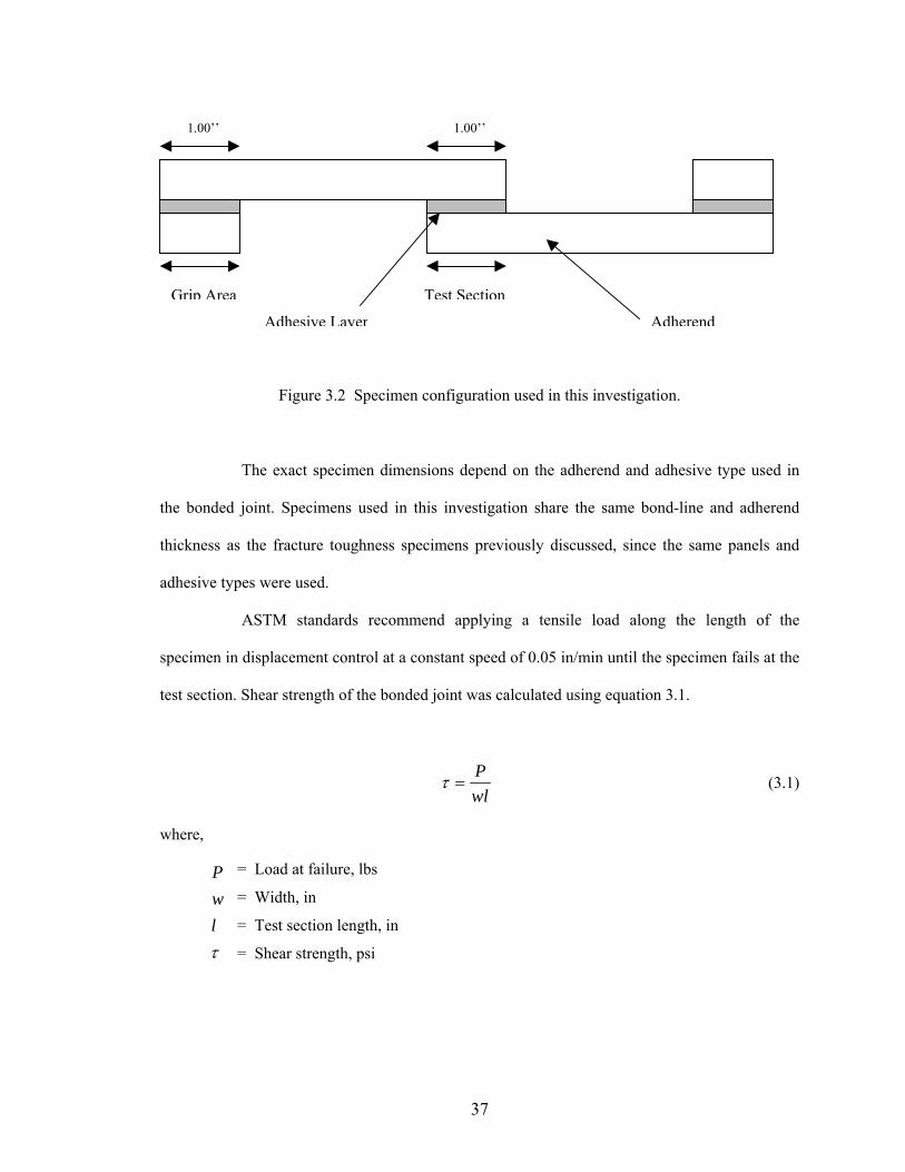
on the recommended specimen configuration. Taking this issue into account, a slightly modified
specimen configuration was used in this investigation, as shown in Figure 3.2.
AdherendAdhesive
Thin layer of adherend damagedThin layer of adhesive left
Figure 3.1 Milling issues of ASTM 3165 recommended specimen configuration.
36
1.00’’ 1.00’’
Adhesive LayerTest SectionGrip Area
Adherend
Figure 3.2 Specimen configuration used in this investigation.
The exact specimen dimensions depend on the adherend and adhesive type used in
the bonded joint. Specimens used in this investigation share the same bond-line and adherend
thickness as the fracture toughness specimens previously discussed, since the same panels and
adhesive types were used.
ASTM standards recommend applying a tensile load along the length of the
specimen in displacement control at a constant speed of 0.05 in/min until the specimen fails at the
test section. Shear strength of the bonded joint was calculated using equation 3.1.
wlP
=τ (3.1)
where,
τlwP = Load at failure, lbs
= Width, in
= Test section length, in
= Shear strength, psi
37
3.2 Specimen Fabrication
The specimen fabrication process for single-lap shear was approached similarly as
fracture toughness specimen fabrication discussed in chapter 2. The same panels along with the
same adhesive types and cure cycles were used in the bonding process. The specimen
configuration introduced in the previous section allows for bonding the adherend and grip
sections separately, thus reducing the machining time and eliminating the imperfections discussed
above. The bond-line thickness was maintained using the same brass spacers along the bonded
region.
The first step in specimen fabrication was to resize the original panels into adherend
sections and grip sections according to the final expected specimen geometric dimensions.
Surface preparation of the bonding areas of the adherend sections and grip sections were done
similarly, using a sandblaster. Utility tape was used to serve a different purpose in this fabrication
process compared to that for fracture toughness specimens. Utility tape was applied to the outside
of the bonding region to remove the excess adhesive when curing under pressure. Figures 3.3a
and 3.3b summarize these steps for a glass adherend bonding process.
Panels were bonded using a bladder press with a pressure of 10 psi following the
same cure cycle process in section 2.2.3. Paste adhesive EA 9394 was cured at room temperature
for five days and film adhesive EA 9628 was cured at 250 0F for one hour. Individual specimens
were then milled, avoiding the spacer location, as shown in Figure 3.4.
Individual specimens were ready for testing once the geometric dimensions and
bond-line thickness were measured. Geometric dimensions were measured using a flat head
caliper, and bond-line thicknesses were measured using a microscope. All the apparatuses were
properly calibrated according to manufacturer standards. Figure 3.5 shows a single-lap shear
specimen ready for testing.
38
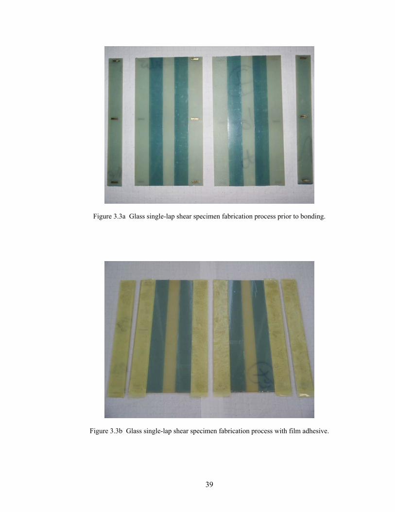
Figure 3.3a Glass single-lap shear specimen fabrication process prior to bonding.
Figure 3.3b Glass single-lap shear specimen fabrication process with film adhesive.
39
Top View
Spacer Location
Side View (Not to Scale)
1.00”
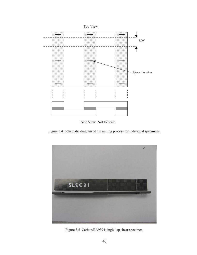
Figure 3.4 Schematic diagram of the milling process for individual specimens.
Figure 3.5 Carbon/EA9394 single-lap shear specimen.
40
3.3 Testing
Single-lap shear testing was conducted in accordance with the ASTM D3165
standard using a 22 kip servo hydraulic with a test rate of 0.05 in/min in displacement control.
Hydraulic clamping grips were used to attach the specimen to the test frame. Attention was given
to proper alignment in order to avoid bending and asymmetric loading. After some trial
specimens, grip pressure was set to 1000 psi. It is important to clamp the specimens in load
control allowing minimum stress in the adhesive gage section of the specimen. Load and actuator
displacement data was collected using TestWorks software with a data acquisition rate of 10 Hz
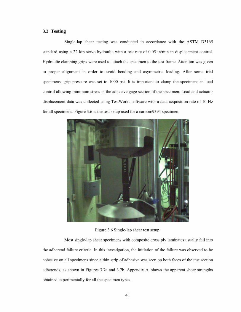
for all specimens. Figure 3.6 is the test setup used for a carbon/9394 specimen.
Figure 3.6 Single-lap shear test setup.
Most single-lap shear specimens with composite cross ply laminates usually fall into
the adherend failure criteria. In this investigation, the initiation of the failure was observed to be
cohesive on all specimens since a thin strip of adhesive was seen on both faces of the test section
adherends, as shown in Figures 3.7a and 3.7b. Appendix A. shows the apparent shear strengths
obtained experimentally for all the specimen types.
41

Figure 3.7a Failure modes of glass/9394-cohesive failure at initiation.
Figure 3.7b Failure modes of carbon/9628-cohesive failure at initiation.
42
CHAPTER 4
FINITE ELEMENT MODELING AND ANALYSIS
Finite element method (FEM) analysis is a crucial part of this investigation since it
serves as a tool in developing the failure load prediction method. FEM is a proven analytical tool
used in the industry mainly to simulate stresses and strains of any structural part given the
material properties and loading configuration. Complexity of the finite element method increases
with the part’s geometry as well as material behavior and meshing technique, since the core of
this method relies on dividing the given part into elements and solving at an elemental scale.
Hence, finer the mesh, the more accurate the results are.
Commercial finite element (FE) codes are readily available to simulate almost any
kind of a structural component. Reliability, cost, and user-friendliness drive the preference of one
code over another. Analytical models using low cost commercial solvers such as MAPLE,
MATHEMATICA, etc. are an alternate approach. The laminated plate theory based analytical
model developed by Huang H. et al. [17] to determine stress and strain distributions of a single-
lap adhesive-bonded composite joint under tension is such an approach. This investigation
required a tool that could determine the strain energy release rate of a cohesive crack, a step
beyond the stress and strain analysis. Fracture Analysis Code 2D (FRANC2D) is a finite element
based software package developed by Cornel Fracture Group that is freely available over the
World Wide Web. FRANC2D has been successfully used as a fracture analysis tool to determine
stress intensity and proved to be reliable [18]. This package was used to model single-lap joint
specimens tested with different adherend-adhesive combinations, as discussed in the previous
chapter. Laminate properties were calculated using the CLASS software introduced in Chapter 2
with laminar properties published in the AGATE database [19]. Manufacturer-published adhesive
properties were used for both adhesive types.
43
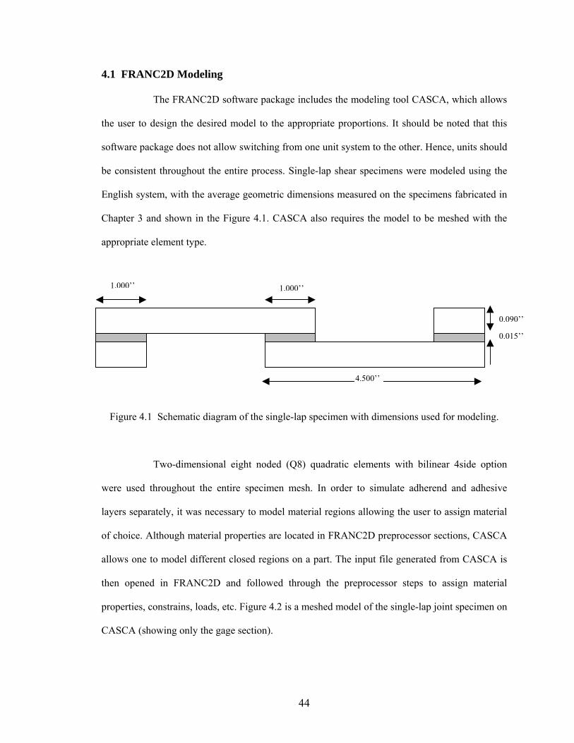
4.1 FRANC2D Modeling
The FRANC2D software package includes the modeling tool CASCA, which allows
the user to design the desired model to the appropriate proportions. It should be noted that this
software package does not allow switching from one unit system to the other. Hence, units should
be consistent throughout the entire process. Single-lap shear specimens were modeled using the
English system, with the average geometric dimensions measured on the specimens fabricated in
Chapter 3 and shown in the Figure 4.1. CASCA also requires the model to be meshed with the
appropriate element type.
1.000’’ 1.000’’
0.015’’
0.090’’
4.500’’
Figure 4.1 Schematic diagram of the single-lap specimen with dimensions used for modeling.
Two-dimensional eight noded (Q8) quadratic elements with bilinear 4side option
were used throughout the entire specimen mesh. In order to simulate adherend and adhesive
layers separately, it was necessary to model material regions allowing the user to assign material
of choice. Although material properties are located in FRANC2D preprocessor sections, CASCA
allows one to model different closed regions on a part. The input file generated from CASCA is
then opened in FRANC2D and followed through the preprocessor steps to assign material
properties, constrains, loads, etc. Figure 4.2 is a meshed model of the single-lap joint specimen on
CASCA (showing only the gage section).
44
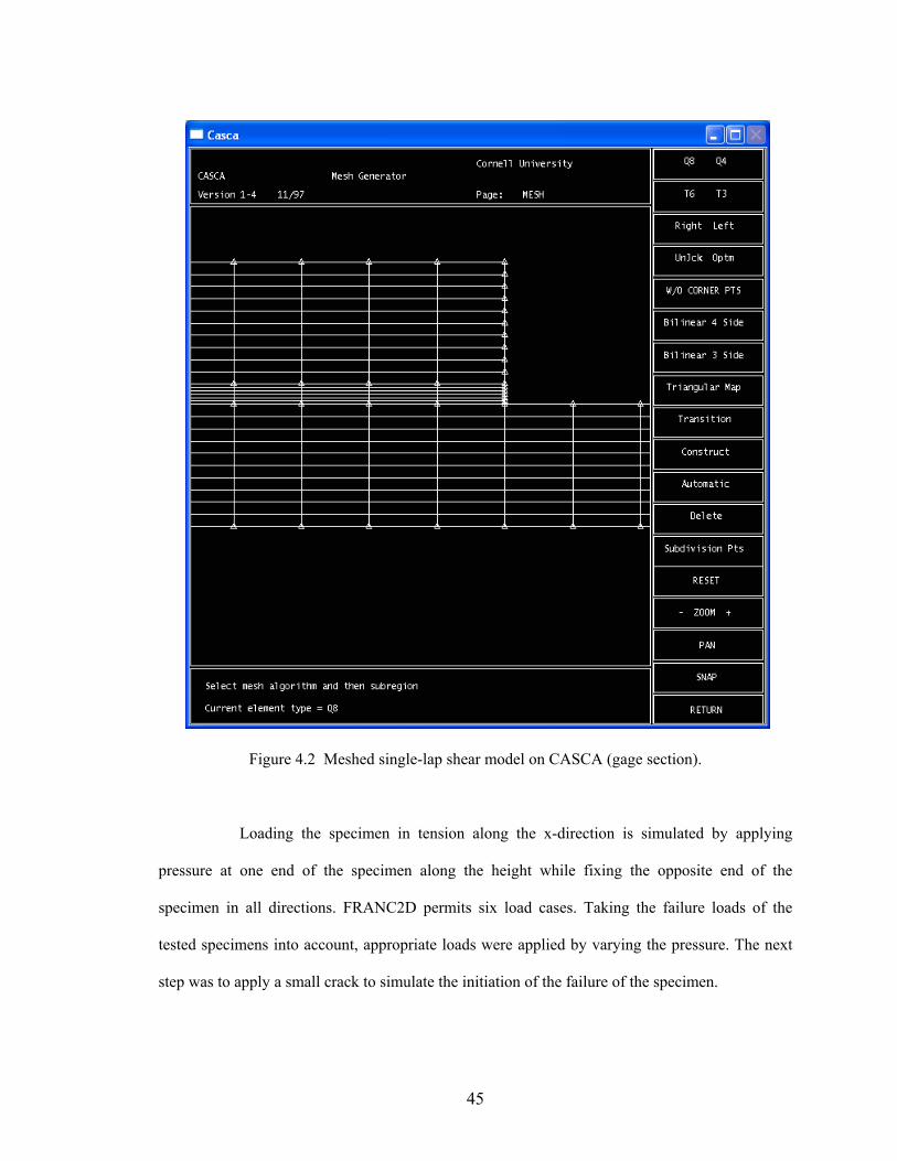
Figure 4.2 Meshed single-lap shear model on CASCA (gage section).
Loading the specimen in tension along the x-direction is simulated by applying
pressure at one end of the specimen along the height while fixing the opposite end of the
specimen in all directions. FRANC2D permits six load cases. Taking the failure loads of the
tested specimens into account, appropriate loads were applied by varying the pressure. The next
step was to apply a small crack to simulate the initiation of the failure of the specimen.
45
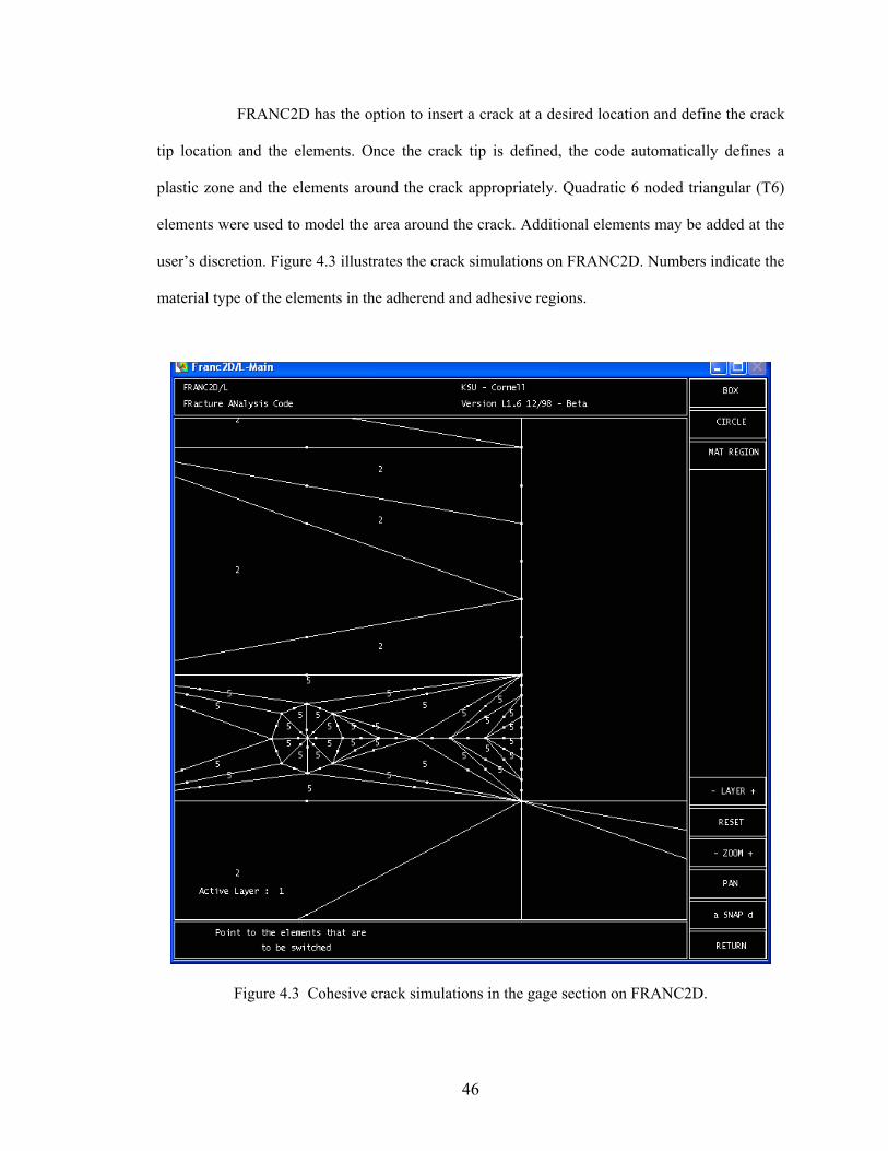
FRANC2D has the option to insert a crack at a desired location and define the crack
tip location and the elements. Once the crack tip is defined, the code automatically defines a
plastic zone and the elements around the crack appropriately. Quadratic 6 noded triangular (T6)
elements were used to model the area around the crack. Additional elements may be added at the
user’s discretion. Figure 4.3 illustrates the crack simulations on FRANC2D. Numbers indicate the
material type of the elements in the adherend and adhesive regions.
Figure 4.3 Cohesive crack simulations in the gage section on FRANC2D.
46

4.2 ASSUMPTIONS
This investigation was limited to linear elastic behavior, hence, all the equations used
to obtain fracture toughness values from experimental methods discussed in previous chapters
reflect linear elasticity. It should be noted that by making the same assumptions, FRANC2D
simulation of the single-lap joint specimens may affect the results to a certain degree. Below is a
list of assumptions made in the modeling and analysis segments of FEM analysis.
• Adherend laminates were modeled with elastic orthotropic material.
• Adhesive region was modeled with elastic isotropic material.
• Elastic behavior was assumed throughout the entire analysis.
• Cohesive failure initiation was assumed.
• Average dimensions of the specimens tested were used for the model.
47

4.3 FRANC2D Analysis
The Analysis segment of the code provides several options to calculate the strain
energy release rate. Modified crack closure technique and J-integral are two popular options.
Since the adhesive and adherends were assumed to behave only in the elastic region, J integral
was used to determine strain energy release rates at the crack tip.
J Integral
J integral is a path-independent contour energy integral formulated by Rice and used for
evaluating fracture toughness of elastic-plastic material [5]. J integral is approximately the same
as the strain energy release rate, G, in the elastic region. Components of the J integral in mode I
and mode II directions are JI and JII, similar to GI and GII. Formulation of the J integral is
summarized in Figure 4.4, with the simplified components assuming small strains.
ds
CrackO
n
X
Y
( )
( )1212
2222
2121
ετ
ετ
hJ
hJ
II
I
=
=
∫Γ ∂∂
−= dsxu
TwdyJ ii
where; is the strain energy density, ∫= ij
ijij dwε
εσ0 jiji nT σ= is the traction vector, and h is the
adhesive thickness
Figure 4.4 Formulation of J integral.
48
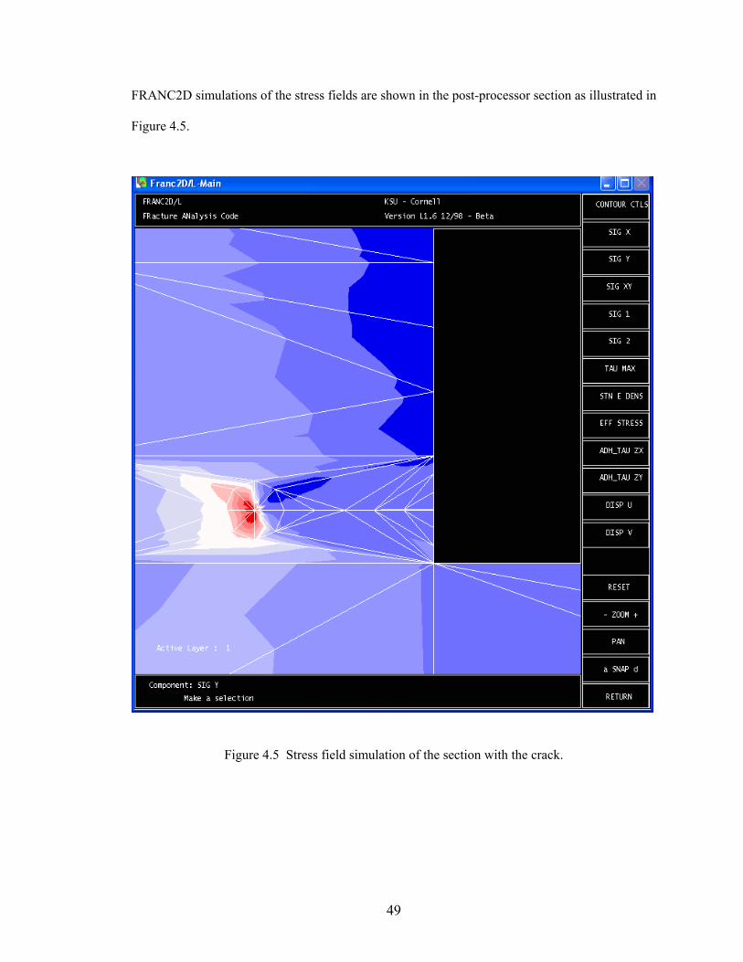
FRANC2D simulations of the stress fields are shown in the post-processor section as illustrated in
Figure 4.5.
Figure 4.5 Stress field simulation of the section with the crack.
49
CHAPTER 5
RESULTS AND DISCUSSION
This chapter presents the results obtained experimentally from mixed-mode fracture
toughness testing and single-lap joint testing. Numerically calculated results using FRANC2D are
also presented. The proposed methodology to predict failure of a bonded joint is illustrated using
a single-lap joint configuration. Adherend effects on mixed-mode fracture toughness results and
the proposed failure prediction method are discussed. In addition the proposed methodology to
predict the failure initiation of an adhesive joint using mixed-mode fracture data is outlined.
5.1 Experimental and Finite Element Result
Mixed-mode fracture toughness curves were generated using the data obtained from
mixed-mode fracture toughness testing. Curves were plotted for the two types of adhesives, EA
9394 and EA 9628. Three types of adherends were used with EA 9394 in mixed-mode testing
resulting in three curves. Two types of adherends were used with EA 9628 thus generating two
curves. Single-lap joint specimens were tested for the two adhesive types as illustrated in Chapter
3. Failure loads obtained were used to determine apparent shear strengths.
Mode-mixity values for the single-lap joint specimens tested were obtained from
FRANC2D. Furthermore, applied load and corresponding strain energy release rates were
calculated for each adhesive-adherend combination single-lap joint specimen using FRANC2D.
Load vs. strain energy release rate values were plotted to obtain the relationship between the
applied load and the strain energy release rate at the joint assuming a small crack.
50
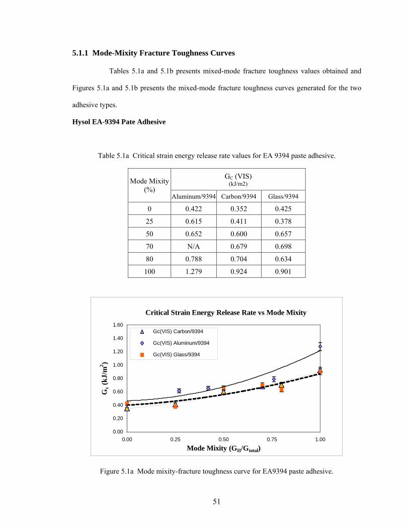
5.1.1 Mode-Mixity Fracture Toughness Curves
Tables 5.1a and 5.1b presents mixed-mode fracture toughness values obtained and
Figures 5.1a and 5.1b presents the mixed-mode fracture toughness curves generated for the two
adhesive types.
Hysol EA-9394 Pate Adhesive
Table 5.1a Critical strain energy release rate values for EA 9394 paste adhesive.
GC (VIS) (kJ/m2) Mode Mixity
(%) Aluminum/9394 Carbon/9394 Glass/9394
0 0.422 0.352 0.425
25 0.615 0.411 0.378
50 0.652 0.600 0.657
70 N/A 0.679 0.698
80 0.788 0.704 0.634
100 1.279 0.924 0.901
Critical Strain Energy Release Rate vs Mode Mixity
0.00
0.20
0.40
0.60
0.80
1.00
1.20
1.40
1.60
0.00 0.25 0.50 0.75 1.00
Mode Mixity (GII/Gtotal)
Gc (
kJ/m
2 )
Gc(VIS) Carbon/9394
Gc(VIS) Aluminum/9394
Gc(VIS) Glass/9394
Figure 5.1a Mode mixity-fracture toughness curve for EA9394 paste adhesive.
51
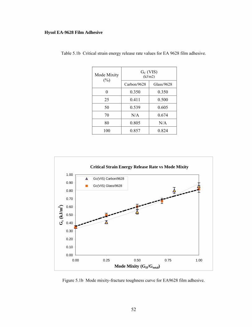
Hysol EA-9628 Film Adhesive
Table 5.1b Critical strain energy release rate values for EA 9628 film adhesive.
GC (VIS) (kJ/m2) Mode Mixity
(%) Carbon/9628 Glass/9628
0 0.350 0.350
25 0.411 0.500
50 0.539 0.605
70 N/A 0.674
80 0.805 N/A
100 0.857 0.824
Critical Strain Energy Release Rate vs Mode Mixity
0.00
0.10
0.20
0.30
0.40
0.50
0.60
0.70
0.80
0.90
1.00
0.00 0.25 0.50 0.75 1.00
Mode Mixity (GII/Gtotal)
Gc (
kJ/m
2 )
Gc(VIS) Carbon/9628
Gc(VIS) Glass/9628
Figure 5.1b Mode mixity-fracture toughness curve for EA9628 film adhesive.
52
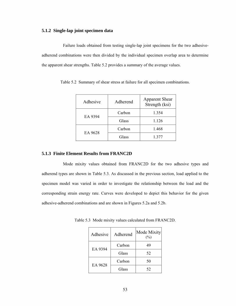
5.1.2 Single-lap joint specimen data
Failure loads obtained from testing single-lap joint specimens for the two adhesive-
adherend combinations were then divided by the individual specimen overlap area to determine
the apparent shear strengths. Table 5.2 provides a summary of the average values.
Table 5.2 Summary of shear stress at failure for all specimen combinations.
Adhesive Adherend Apparent Shear Strength (ksi)
Carbon 1.354 EA 9394
Glass 1.126
Carbon 1.468 EA 9628
Glass 1.377
5.1.3 Finite Element Results from FRANC2D
Mode mixity values obtained from FRANC2D for the two adhesive types and
adherend types are shown in Table 5.3. As discussed in the previous section, load applied to the
specimen model was varied in order to investigate the relationship between the load and the
corresponding strain energy rate. Curves were developed to depict this behavior for the given
adhesive-adherend combinations and are shown in Figures 5.2a and 5.2b.
Table 5.3 Mode mixity values calculated from FRANC2D.
Adhesive Adherend Mode Mixity (%)
Carbon 49 EA 9394
Glass 52
Carbon 50 EA 9628
Glass 52
53

Load vs. Strain Energy Release Rate
0.0
0.2
0.4
0.6
0.8
1.0
1.2
500 750 1000 1250 1500
Load, lbf
Stra
in E
nerg
y R
elea
se R
ate,
Gc
(kJ/
m2 )
Carbon/9394Glass/9394
Figure 5.2a Load vs. strain energy release rate for EA 9394 from FRANC2D.
Load vs. Strain Energy Release Rate
0.0
0.2
0.4
0.6
0.8
1.0
1.2
500 750 1000 1250 1500 1750Load, lbf
Stra
in E
nerg
y R
elea
se R
ate,
Gc
(kJ/
m2 )
Carbon/9628Glass/9628
Figure 5.2b Load vs. strain energy release rate for EA 9628 from FRANC2D.
54
5.2 Failure Initiation Prediction
Failure initiation prediction for the single-lap joint specimen configurations was
approached by first generating a single mixed-mode fracture toughness curve for each adhesive
type. This was achieved by taking the average strain energy rate values for the two composite
adherend types used to generate the mode-mixity fracture toughness curve and plotting a single
curve for the given adhesive type. As shown in Figures 5.1a and 5.1b, curves generated from
glass and carbon adherends coincide with each other for the two adhesive types. However, the
curve generated by aluminum adherends is considerably higher than the curves generated by
composite adherends. Aluminum was only used with the EA 9493 paste adhesive and considered
separately.
Mode-mixity values calculated using FRANC2D for the single-lap joint specimens
were plotted on the appropriate adhesive mode-mixity fracture toughness curve to determine the
critical strain energy release rate or fracture toughness, as shown in Figures 5.3a and 5.3b. Figure
5.4 illustrates the mode-mixity fracture toughness curve generated using aluminum adherends.
Table 5.4 is a summary of the fracture toughness values corresponding to the mode mixities for
the given single-lap joint configurations.
The fracture toughness or critical strain energy release rate values obtained were then
referred back to the load vs. strain energy release rate curves presented in Figures 5.2a and 5.2b to
determine failure load. Figures 5.5a and 5.5b illustrate this step. Corresponding failure load
values were then converted to apparent shear strength. Predicted failure values are then compared
with the apparent shear strengths obtained experimentally from single-lap joint testing for the two
adhesive types as depicted in Figures 5.6a and 5.6b.
55
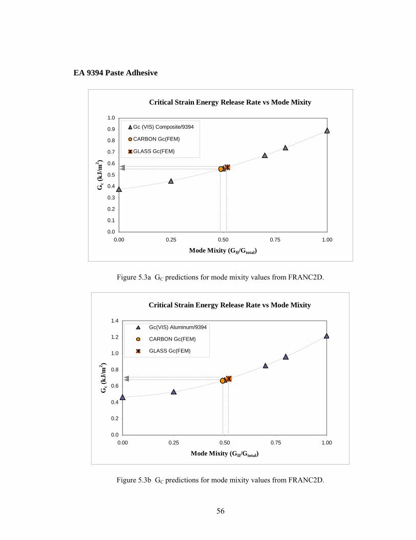
EA 9394 Paste Adhesive
Critical Strain Energy Release Rate vs Mode Mixity
0.0
0.1
0.2
0.3
0.4
0.5
0.6
0.7
0.8
0.9
1.0
0.00 0.25 0.50 0.75 1.00
Mode Mixity (GII/Gtotal)
Gc (
kJ/m
2 )
Gc (VIS) Composite/9394
CARBON Gc(FEM)
GLASS Gc(FEM)
Figure 5.3a GC predictions for mode mixity values from FRANC2D.
Critical Strain Energy Release Rate vs Mode Mixity
0.0
0.2
0.4
0.6
0.8
1.0
1.2
1.4
0.00 0.25 0.50 0.75 1.00
Mode Mixity (GII/Gtotal)
Gc (
kJ/m
2 )
Gc(VIS) Aluminum/9394
CARBON Gc(FEM)
GLASS Gc(FEM)
Figure 5.3b GC predictions for mode mixity values from FRANC2D.
56
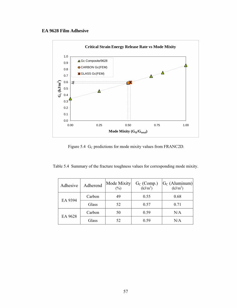
EA 9628 Film Adhesive
Critical Strain Energy Release Rate vs Mode Mixity
0.0
0.1
0.2
0.3
0.4
0.5
0.6
0.7
0.8
0.9
1.0
0.00 0.25 0.50 0.75 1.00
Mode Mixity (GII/Gtotal)
Gc (
kJ/m
2 )Gc Composite/9628
CARBON Gc(FEM)
GLASS Gc(FEM)
Figure 5.4 GC predictions for mode mixity values from FRANC2D.
Table 5.4 Summary of the fracture toughness values for corresponding mode mixity.
Adhesive Adherend Mode Mixity (%)
GC (Comp.) (kJ/m2)
GC (Aluminum) (kJ/m2)
Carbon 49 0.55 0.68 EA 9394
Glass 52 0.57 0.71
Carbon 50 0.59 N/A EA 9628
Glass 52 0.59 N/A
57
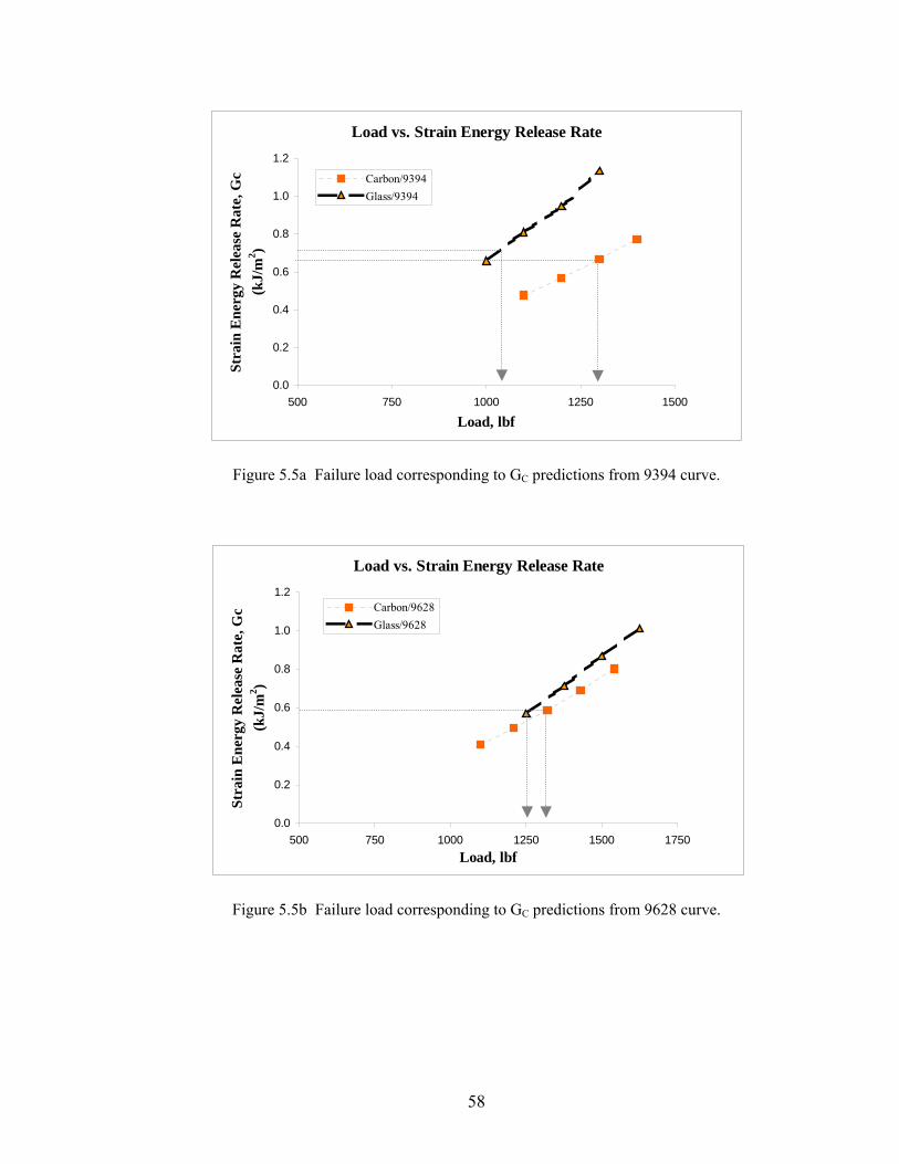
Load vs. Strain Energy Release Rate
0.0
0.2
0.4
0.6
0.8
1.0
1.2
500 750 1000 1250 1500
Load, lbf
Stra
in E
nerg
y R
elea
se R
ate,
Gc
(kJ/
m2 )
Carbon/9394Glass/9394
Figure 5.5a Failure load corresponding to GC predictions from 9394 curve.
Load vs. Strain Energy Release Rate
0.0
0.2
0.4
0.6
0.8
1.0
1.2
500 750 1000 1250 1500 1750Load, lbf
Stra
in E
nerg
y R
elea
se R
ate,
Gc
(kJ/
m2 )
Carbon/9628Glass/9628
Figure 5.5b Failure load corresponding to GC predictions from 9628 curve.
58
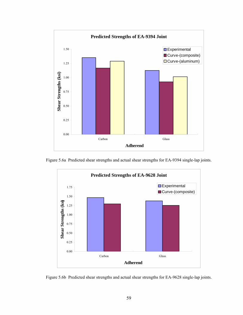
Predicted Strengths of EA-9394 Joint
0.00
0.25
0.50
0.75
1.00
1.25
1.50
Carbon Glass
Adherend
Shea
r St
reng
ths (
ksi)
ExperimentalCurve-(composite)Curve-(aluminum)
Figure 5.6a Predicted shear strengths and actual shear strengths for EA-9394 single-lap joints.
Predicted Strengths of EA-9628 Joint
0.00
0.25
0.50
0.75
1.00
1.25
1.50
1.75
Carbon Glass
Adherend
Shea
r St
reng
ths (
ksi )
ExperimentalCurve-(composite)
Figure 5.6b Predicted shear strengths and actual shear strengths for EA-9628 single-lap joints.
59
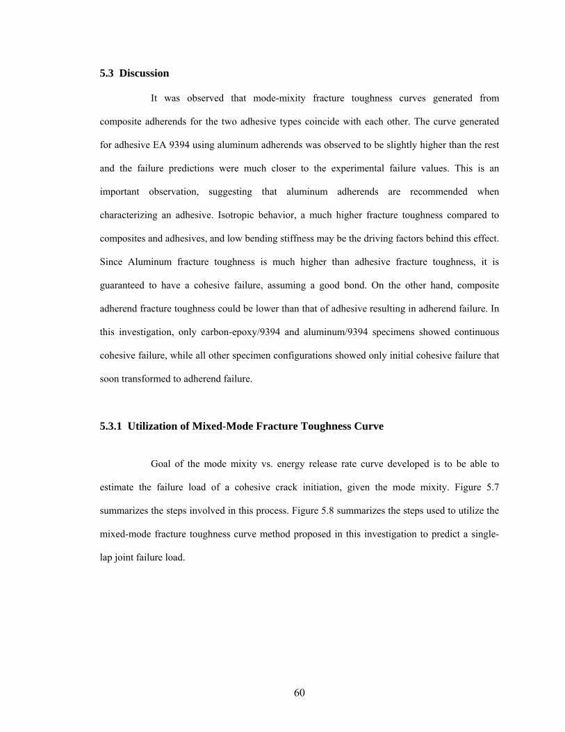
5.3 Discussion
It was observed that mode-mixity fracture toughness curves generated from
composite adherends for the two adhesive types coincide with each other. The curve generated
for adhesive EA 9394 using aluminum adherends was observed to be slightly higher than the rest
and the failure predictions were much closer to the experimental failure values. This is an
important observation, suggesting that aluminum adherends are recommended when
characterizing an adhesive. Isotropic behavior, a much higher fracture toughness compared to
composites and adhesives, and low bending stiffness may be the driving factors behind this effect.
Since Aluminum fracture toughness is much higher than adhesive fracture toughness, it is
guaranteed to have a cohesive failure, assuming a good bond. On the other hand, composite
adherend fracture toughness could be lower than that of adhesive resulting in adherend failure. In
this investigation, only carbon-epoxy/9394 and aluminum/9394 specimens showed continuous
cohesive failure, while all other specimen configurations showed only initial cohesive failure that
soon transformed to adherend failure.
5.3.1 Utilization of Mixed-Mode Fracture Toughness Curve
Goal of the mode mixity vs. energy release rate curve developed is to be able to
estimate the failure load of a cohesive crack initiation, given the mode mixity. Figure 5.7
summarizes the steps involved in this process. Figure 5.8 summarizes the steps used to utilize the
mixed-mode fracture toughness curve method proposed in this investigation to predict a single-
lap joint failure load.
60
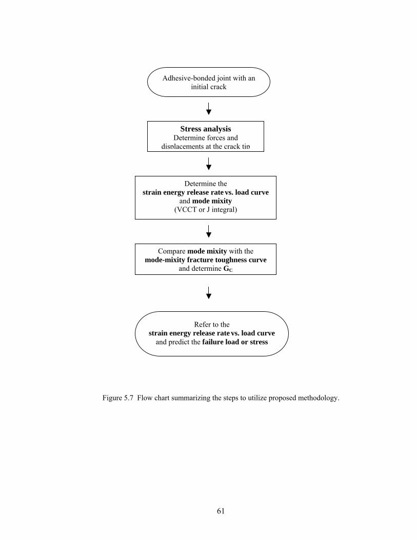
Adhesive-bonded joint with an
initial crack
Stress analysis Determine forces and
displacements at the crack tip
Determine the strain energy release rate vs. load curve
and mode mixity (VCCT or J integral)
Compare mode mixity with the mode-mixity fracture toughness curve
and determine GC
Refer to the strain energy release rate vs. load curve
and predict the failure load or stress
Figure 5.7 Flow chart summarizing the steps to utilize proposed methodology.
61
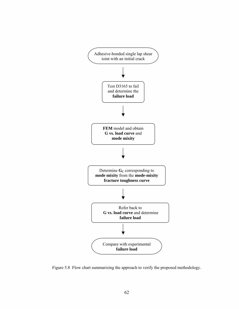
Adhesive-bonded single lap shear joint with an initial crack
Test D3165 to fail and determine the
failure load
FEM model and obtain G vs. load curve and
mode mixity
Determine GC corresponding to mode mixity from the mode-mixity
fracture toughness curve
Refer back to G vs. load curve and determine
failure load
Compare with experimental
failure load
Figure 5.8 Flow chart summarizing the approach to verify the proposed methodology.
62
CHAPTER 6
CONCLUSIONS AND RECOMMENDATIONS
Several conclusions were drawn from this investigation ranging from the process
stage and testing methods to the analysis, summarizing the entire investigation.
Recommendations were made based on the conclusions with the intention of serving as a
stepping-stone for future work related to mixed-mode fracture toughness of adhesives.
6.1 Conclusions
• Two types of adhesivesEA9394 paste adhesive and EA9628 film adhesivewere
selected for the investigation, based on their wide use in the industry.
• Three types of adherends were selected: Aluminum 2024-T3, Carbon-epoxy, and
E-glass. Composite adherends selection was based on their wide use in the industry
as adherends in single-lap adhesive joint testing, while Aluminum was selected to
study the effect of adherend types on adhesive characterization.
• Mode I and mixed-mode testing were conducted per ASTM D5528 and D6671
standards, while mode II testing was conducted using a three-point bend per
SACMA standard.
• Mixed-mode bending test suggested by the ASTM standard for mixed-mode
fracture toughness was somewhat inconvenient to use at higher mode mixities,
since the hinges that are bonded to the specimen attaching the fixture tend to fail
the bonded composite layer of the adherend because of the high load.
• Mixed-mode fracture toughness curves were generated for adhesives EA 9394 and
EA 9628. Curves generated using two composite adherends for the two adhesive
63
types were fairly consistent with each other, while the curve generated from
aluminum adherend was slightly higher.
• Adhesive-bonded single-lap shear specimens were tested per ASTM D3165
standard with the two composite adherends selected for the two adhesive types to
obtain the failure loads that can be used to compare with predictions made by the
proposed method via a mixed-mode fracture toughness curve.
• Adherend failure was observed in all single-lap shear specimens tested. However,
failure initiation was determined to be cohesive. Hence, FEM analysis was
conducted on a cohesive crack initiation.
• FRANC2D was used as the main analysis code since it was freely available and has
been used successfully for fracture analysis.
• J integral was used in FRANC2D to determine the strain energy release rates at the
crack tip for the applied load. Load vs. strain energy release rate curves were
developed ranging the applied load and calculating the corresponding strain energy
release.
• Failure loads obtained experimentally were about 15% off from those predicted by
the curves generated using composite adherends.
• Failure loads obtained experimentally were about 5% off from those predicted by
the response curves generated using aluminum adherends. Aluminum adherends
were only used to generate a curve for EA 9394 paste adhesive.
• Utilization of the proposed methodology based on the mode-mixity fracture
toughness curve for certain adhesives is summarized, followed by a conformation
using a single-lap joint.
64
6.2 Recommendations for Future Work
• Approach adherend selection keeping in mind the fracture toughness of both the
adhesive and adherend, allowing them to, not only initiate cohesively but also
propagate cohesively since fracture toughness varies with crack length.
• Use aluminum 20224-T3 adherends with an anodized surface, which proved to be
the choice for adhesive characterization to develop curves as opposed to composite
adherends.
• Explore alternate testing methods for mixed-mode fracture toughness
determination.
• Generate more data points along the response curve to offset the irregularities and
to make the curve more accurate.
• Extend FEM analysis to confirm the mode-mixity fracture toughness curves
generated experimentally.
• Use a high-end FEM software package for generating the load vs. strain energy
release rate curves to compliment the mode-mixity fracture toughness curves
developed experimentally.
• Extend the proposed methodology to different environmental conditions and
compare this to the environmental effects on the proposed methodology.
• Investigate crack initiation by fatigue effect; compare the mixed-mode fracture
toughness curves generated with those by static loading.
• Explore the effect of initial crack length on strain energy release rate at crack tip
using FEM analysis.
• Further explore the relationship between load and strain energy release rate maybe
further explored by extending the curves generated from FEM model, looking for a
possible trend.
65

REFERENCES
66
[1] “Primary Adhesively Bonded Structure Technology (PABST) Industry Review”, Page 166-204, September 14-16, 1977.
[2] Ullah, Md. H., “Analysis of Cohesive Failure of Adhesive Bonded
Composite Joints”, M.S. Thesis, Dept. of Mechanical Engineering, Wichita State University, Wichita, KS, USA, 2002.
[3] “Standard Test Method for Strength Properties of Adhesives in Shear by
Tension Loading of Single Lap Joint Laminated Assemblies”, Annual Book of ASTM Standards, 2000, Vol. 15.06 [CD-ROM].
[4] Ramaswamy, S. and Tippur, H. V. and Xu, L., “Mixed mode Fracture
Deformations Studied Using A Modified Flexural Specimen and Coherent Gradient Sensing”, Experimental Mechanics, SAGE Social Science Collection, Sept. 1993.
[5] Kossira, H. and Weerts, U, “Mixed Mode Fracture Characterization of
Adhesive Joints”, International Council of Aeronautical Science, 2000 [6] Pirondi, A. and Nicoletto, G., “Mixed Mode Fracture Envelope of a
Structural Adhesive”, Department of Industrial Engineering, University of Parma, Italy, June 2001.
[7] Nairn, A. J., “Energy Release Rate Analysis for Adhesive and Laminate
Double Cantilever Beam specimens emphasizing the effect of residual stresses”, International Journal of Adhesion & Adhesives, Vol. 20, 1999, pp 59-70.
[8] Moore, D.R. and Williams J. G., “A Protocol for Determination of the
Adhesive Fracture Toughness by Peel Testing of Flexible Laminates”, June 2000, URL: http://www3.imperial.ac.uk/pls/portallive/docs/1/41494.pdf [cited 12 December 2004].
[9] Yang, Q. D., Thouless, M. D. and Ward, S. M., “Elastic-Plastic Mode-II
Fracture of Adhesive Joints”, May 2000, URL: http://www-personal.engin.umich.edu/~thouless/Mode2.pdf [cited 15 Dec. 2004].
[10] Krueger, R., “A Shell/3D Modeling Technique for Delaminations in
Composite Laminates”, Proceedings of the American Society for Composites, 14th Technical Conference, Technomic Publishing, ISBN 1-56676-791-1, pp. 843-852, 1999.
[11] Bardis, J. D. and Kedward, K. T., “Surface Preparation Effects on Mode I
Testing of Adhesively Bonded Composite Joints”, Journal of Composite Technology and Research, Vol. 24, Issue 1, Jan. 2002.
67
[12] “Standard Method for Mixed Mode I-Mode II Interlaminar Fracture Toughness of Unidirectional Fiber Reinforced Polymer Matrix Composites”, Annual Book of ASTM Standards, Vol. 15.06, 2001 [CD-ROM].
[13] Hashemi, S., Kinloch, A. J. and Williams, G., “Mixed-Mode Fracture in
Fiber- Polymer Composite Laminates”, Composite Materials: Fatigue and Fracture, ASTM STP 1110, 1999.
[14] Anderson, T. L., “Fracture Mechanics: Fundamentals and Applications”, 2nd
edition, CRC Press, pp. 44-46, 1995. [15] “Standard Test Method for Mode I Interlaminar Fracture Toughness of
Unidirectional Fiber-Reinforced Polymer Matrix Composites”, Annual Book of ASTM Standards, Vol. 15.06, 2001 [CD-ROM].
[16] “Standard Test Method for Mode II Interlaminar Fracture Toughness of
Unidirectional Fiber-Reinforced Polymer Matrix Composites”, SACMA BMS 8-276F, 2000.
[17] Huang, H., Yang, C., Tomblin, J. and Harter, P., “Stress and Failure
Analysis of Adhesive-Bonded Composite Joints using ASTM D3165 Specimens” Journal of Composites Technology and Research Vol. 24, Issue 2, April 2002.
[18] Cope, D. A., Lacy, T. E., “Modeling Mechanical Fasteners in Lap Joints for
Stress Intensity Determination”, Joint Council on Aging Aircraft, Aging Aircraft Conference, 2000.
[19] B-Basis Design Allowables for Epoxy-Based Prepreg, Advanced General
Aviation Transport Experiments (AGATE), 2001 URL: http://www.niar.wichita.edu/agate [cited 10 Oct. 2005].
[20] Reeder, R. J and Crews, R. Jr., “Mixed mode Bending Method for
Delamination Testing”, AA Journal, Vol. 28, Number 7, pp. 1270-1276, July 1990.
[21] Guess, T. R., Reedy, Stavig, M. E., “Mechanical Properties of Hysol EA-
9394 Structural Adhesive”, Sandia Report, SAND95-0229, Feb. 1995.
68

APPENDIX
69
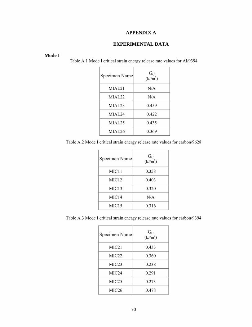
APPENDIX A
EXPERIMENTAL DATA
Mode I Table A.1 Mode I critical strain energy release rate values for Al/9394
Specimen Name GC (kJ/m2)
MIAL21 N/A
MIAL22 N/A
MIAL23 0.459
MIAL24 0.422
MIAL25 0.435
MIAL26 0.369
Table A.2 Mode I critical strain energy release rate values for carbon/9628
Specimen Name GC (kJ/m2)
MIC11 0.358
MIC12 0.403
MIC13 0.320
MIC14 N/A
MIC15 0.316
Table A.3 Mode I critical strain energy release rate values for carbon/9394
Specimen Name GC (kJ/m2)
MIC21 0.433
MIC22 0.360
MIC23 0.238
MIC24 0.291
MIC25 0.273
MIC26 0.478
70
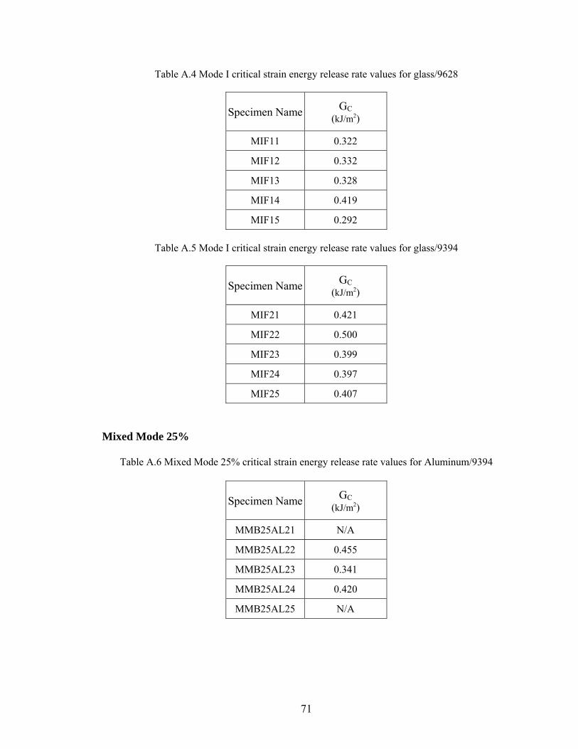
Table A.4 Mode I critical strain energy release rate values for glass/9628
Specimen Name GC (kJ/m2)
MIF11 0.322
MIF12 0.332
MIF13 0.328
MIF14 0.419
MIF15 0.292
Table A.5 Mode I critical strain energy release rate values for glass/9394
Specimen Name GC (kJ/m2)
MIF21 0.421
MIF22 0.500
MIF23 0.399
MIF24 0.397
MIF25 0.407
Mixed Mode 25%
Table A.6 Mixed Mode 25% critical strain energy release rate values for Aluminum/9394
Specimen Name GC (kJ/m2)
MMB25AL21 N/A
MMB25AL22 0.455
MMB25AL23 0.341
MMB25AL24 0.420
MMB25AL25 N/A
71
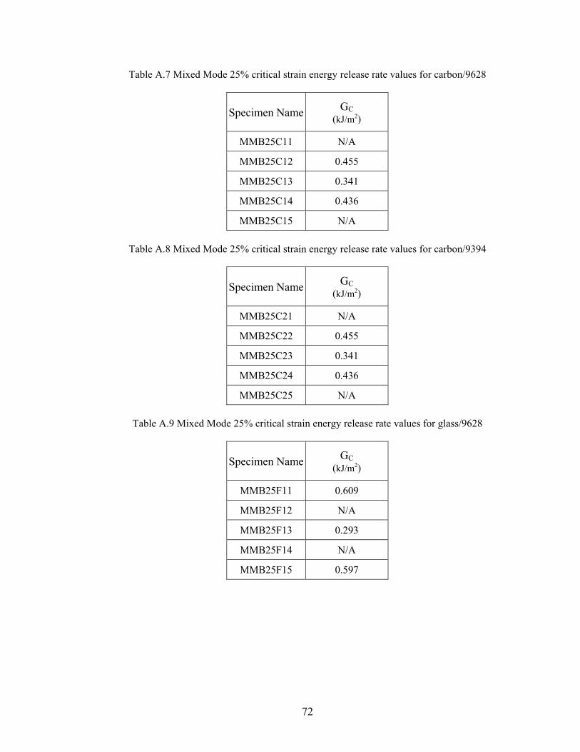
Table A.7 Mixed Mode 25% critical strain energy release rate values for carbon/9628
Specimen Name GC (kJ/m2)
MMB25C11 N/A
MMB25C12 0.455
MMB25C13 0.341
MMB25C14 0.436
MMB25C15 N/A
Table A.8 Mixed Mode 25% critical strain energy release rate values for carbon/9394
Specimen Name GC (kJ/m2)
MMB25C21 N/A
MMB25C22 0.455
MMB25C23 0.341
MMB25C24 0.436
MMB25C25 N/A
Table A.9 Mixed Mode 25% critical strain energy release rate values for glass/9628
Specimen Name GC (kJ/m2)
MMB25F11 0.609
MMB25F12 N/A
MMB25F13 0.293
MMB25F14 N/A
MMB25F15 0.597
72
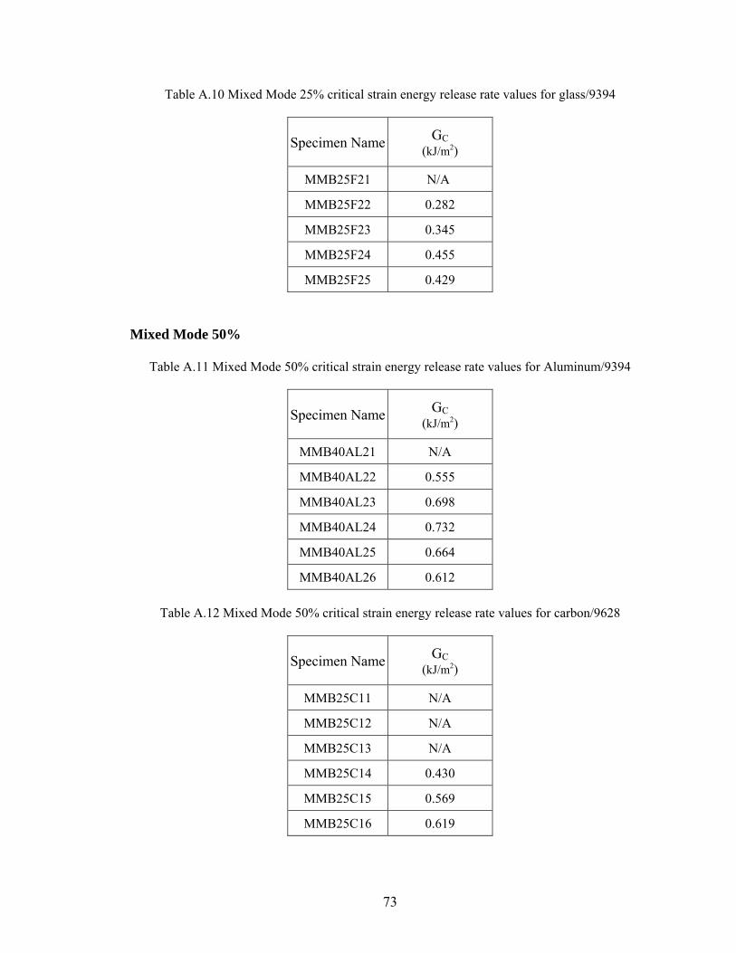
Table A.10 Mixed Mode 25% critical strain energy release rate values for glass/9394
Specimen Name GC (kJ/m2)
MMB25F21 N/A
MMB25F22 0.282
MMB25F23 0.345
MMB25F24 0.455
MMB25F25 0.429 Mixed Mode 50%
Table A.11 Mixed Mode 50% critical strain energy release rate values for Aluminum/9394
Specimen Name GC (kJ/m2)
MMB40AL21 N/A
MMB40AL22 0.555
MMB40AL23 0.698
MMB40AL24 0.732
MMB40AL25 0.664
MMB40AL26 0.612
Table A.12 Mixed Mode 50% critical strain energy release rate values for carbon/9628
Specimen Name GC (kJ/m2)
MMB25C11 N/A
MMB25C12 N/A
MMB25C13 N/A
MMB25C14 0.430
MMB25C15 0.569
MMB25C16 0.619
73

Table A.13 Mixed Mode 50% critical strain energy release rate values for carbon/9394
Specimen Name GC (kJ/m2)
MMB50C21 0.666
MMB50C22 0.683
MMB50C23 0.514
MMB50C24 NA
MMB50C25 0.538
Table A.14 Mixed Mode 50% critical strain energy release rate values for glass/9628
Specimen Name GC (kJ/m2)
MMB50F11 N/A
MMB50F12 0.678
MMB50F13 0.542
MMB50F14 0.542
MMB50F15 0.661
Table A.15 Mixed Mode 50% critical strain energy release rate values for glass/9394
Specimen Name GC (kJ/m2)
MMB50F21 0.539
MMB50F22 0.757
MMB50F23 0.686
MMB50F24 0.639
MMB50F25 0.666
74
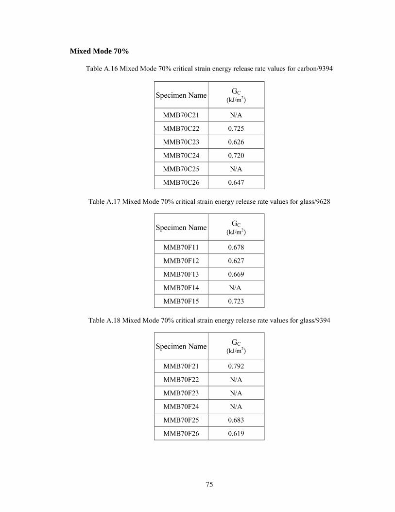
Mixed Mode 70%
Table A.16 Mixed Mode 70% critical strain energy release rate values for carbon/9394
Specimen Name GC (kJ/m2)
MMB70C21 N/A
MMB70C22 0.725
MMB70C23 0.626
MMB70C24 0.720
MMB70C25 N/A
MMB70C26 0.647
Table A.17 Mixed Mode 70% critical strain energy release rate values for glass/9628
Specimen Name GC (kJ/m2)
MMB70F11 0.678
MMB70F12 0.627
MMB70F13 0.669
MMB70F14 N/A
MMB70F15 0.723
Table A.18 Mixed Mode 70% critical strain energy release rate values for glass/9394
Specimen Name GC (kJ/m2)
MMB70F21 0.792
MMB70F22 N/A
MMB70F23 N/A
MMB70F24 N/A
MMB70F25 0.683
MMB70F26 0.619
75

Mixed Mode 80%
Table A.19 Mixed Mode 80% critical strain energy release rate values for Aluminum/9394
Specimen Name GC (kJ/m2)
MMB80AL21 0.912
MMB80AL22 N/A
MMB80AL23 0.676
MMB80AL24 0.740
MMB80AL25 0.790
MMB80AL26 0.735
Table A.20 Mixed Mode 80% critical strain energy release rate values for carbon/9628
Specimen Name GC (kJ/m2)
MMB80C11 0.671
MMB80C12 0.814
MMB80C13 N/A
MMB80C14 0.929
MMB80C15 N/A
Table A.21 Mixed Mode 80% critical strain energy release rate values for carbon/9394
Specimen Name GC (kJ/m2)
MMB80C21 N/A
MMB80C22 0.529
MMB80C23 0.584
MMB80C24 N/A
MMB80C25 0.696
MMB80C26 0.713
76
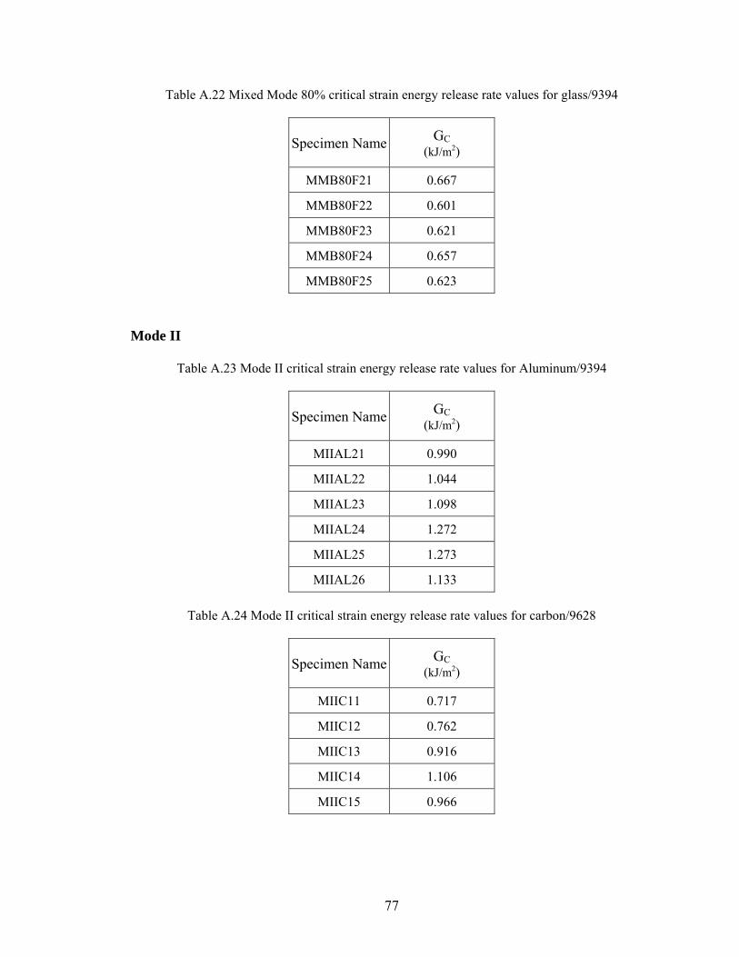
Table A.22 Mixed Mode 80% critical strain energy release rate values for glass/9394
Specimen Name GC (kJ/m2)
MMB80F21 0.667
MMB80F22 0.601
MMB80F23 0.621
MMB80F24 0.657
MMB80F25 0.623
Mode II
Table A.23 Mode II critical strain energy release rate values for Aluminum/9394
Specimen Name GC (kJ/m2)
MIIAL21 0.990
MIIAL22 1.044
MIIAL23 1.098
MIIAL24 1.272
MIIAL25 1.273
MIIAL26 1.133
Table A.24 Mode II critical strain energy release rate values for carbon/9628
Specimen Name GC (kJ/m2)
MIIC11 0.717
MIIC12 0.762
MIIC13 0.916
MIIC14 1.106
MIIC15 0.966
77
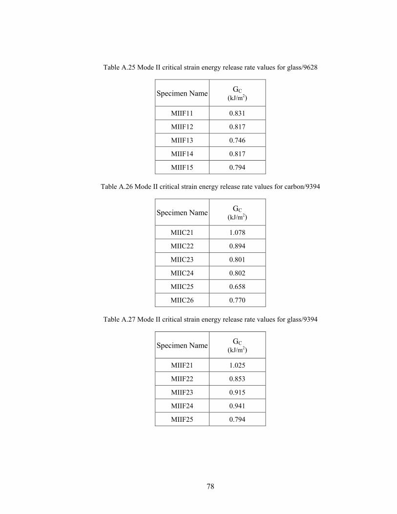
Table A.25 Mode II critical strain energy release rate values for glass/9628
Specimen Name GC (kJ/m2)
MIIF11 0.831
MIIF12 0.817
MIIF13 0.746
MIIF14 0.817
MIIF15 0.794
Table A.26 Mode II critical strain energy release rate values for carbon/9394
Specimen Name GC (kJ/m2)
MIIC21 1.078
MIIC22 0.894
MIIC23 0.801
MIIC24 0.802
MIIC25 0.658
MIIC26 0.770
Table A.27 Mode II critical strain energy release rate values for glass/9394
Specimen Name GC (kJ/m2)
MIIF21 1.025
MIIF22 0.853
MIIF23 0.915
MIIF24 0.941
MIIF25 0.794
78
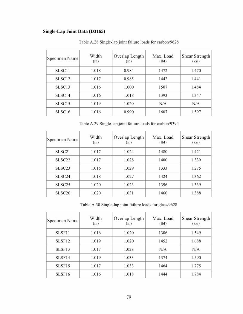
Single-Lap Joint Data (D3165)
Table A.28 Single-lap joint failure loads for carbon/9628
Specimen Name Width (in)
Overlap Length (in)
Max. Load (lbf)
Shear Strength (ksi)
SLSC11 1.018 0.984 1472 1.470
SLSC12 1.017 0.985 1442 1.441
SLSC13 1.016 1.000 1507 1.484
SLSC14 1.016 1.018 1393 1.347
SLSC15 1.019 1.020 N/A N/A
SLSC16 1.016 0.990 1607 1.597
Table A.29 Single-lap joint failure loads for carbon/9394
Specimen Name Width (in)
Overlap Length (in)
Max. Load (lbf)
Shear Strength (ksi)
SLSC21 1.017 1.024 1480 1.421
SLSC22 1.017 1.028 1400 1.339
SLSC23 1.016 1.029 1333 1.275
SLSC24 1.018 1.027 1424 1.362
SLSC25 1.020 1.023 1396 1.339
SLSC26 1.020 1.031 1460 1.388
Table A.30 Single-lap joint failure loads for glass/9628
Specimen Name Width (in)
Overlap Length (in)
Max. Load (lbf)
Shear Strength (ksi)
SLSF11 1.016 1.020 1306 1.549
SLSF12 1.019 1.020 1452 1.688
SLSF13 1.017 1.028 N/A N/A
SLSF14 1.019 1.033 1374 1.590
SLSF15 1.017 1.033 1464 1.775
SLSF16 1.016 1.018 1444 1.784
79
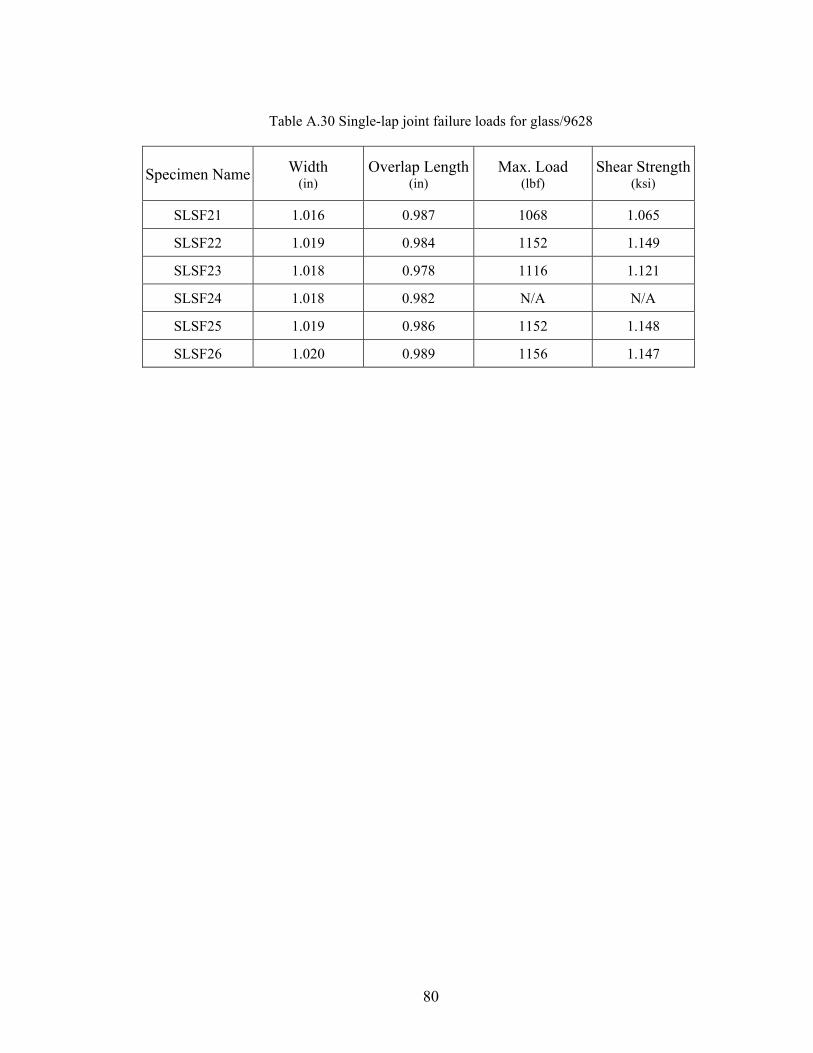
Table A.30 Single-lap joint failure loads for glass/9628
Specimen Name Width (in)
Overlap Length (in)
Max. Load (lbf)
Shear Strength (ksi)
SLSF21 1.016 0.987 1068 1.065
SLSF22 1.019 0.984 1152 1.149
SLSF23 1.018 0.978 1116 1.121
SLSF24 1.018 0.982 N/A N/A
SLSF25 1.019 0.986 1152 1.148
SLSF26 1.020 0.989 1156 1.147
80