prediction learning in robotic manipulation
TRANSCRIPT

Prediction learningin robotic manipulation
by
Marek Kopicki
A thesis submitted to
The University of Birmingham
for the degree of
Doctor Of Philosophy
Computer Science
The University of Birmingham
April 2010

iii
Abstract
This thesis addresses an important problem in robotic manipulation, which is the ability to
predict how objects behave under manipulative actions. This ability is useful for planning of
object manipulations. Physics simulators can be used to do this, but they model many kinds
of object interactions poorly, and unless there is a precise description of an object’s properties
their predictions may be unreliable. An alternative is to learn a model for objects by interacting
with them. This thesis specifically addresses the problem of learning to predict the interactions
of rigid bodies in a probabilistic framework, and demonstrates results in the domain of robotic
push manipulation. During training, a robotic manipulator applies pushes to objects and learns to
predict their resulting motions. The learning does not make explicit use of physics knowledge, nor
is it restricted to domains with any particular physical properties.
The prediction problem is posed in terms of estimating probability densities over the possible
rigid body transformations of an entire object as well as parts of an object under a known action.
Density estimation is useful in that it enables predictions with multimodal outcomes, but it also
enables compromise predictions for multiple combined expert predictors in a product of experts
architecture. It is shown that a product of experts architecture can be learned and that it can
produce generalization with respect to novel actions and object shapes, outperforming in most
cases an approach based on regression.
An alternative, non-learning, method of prediction is also presented, in which a simplified
physics approach uses the minimum energy principle together with a particle-based representation
of the object. A probabilistic formulation enables this simplified physics predictor to be combined
with learned predictors in a product of experts.
The thesis experimentally compares the performance of product of densities, regression,
and simplified physics approaches. Performance is evaluated through a combination of virtual
experiments in a physics simulator, and real experiments with a 5-axis arm equipped with a simple,
rigid finger and a vision system used for tracking the manipulated object.

iv
Acknowledgments
First of all, I would like to thank my supervisor Jeremy Wyatt. This thesis would have never
been possible without his support and encouragement. Also, many ideas in this thesis were born
during discussions with Jeremy.
I owe much to Aaron Sloman who convinced me that robotics could be even my life
endeavour. I am also grateful to Aaron for many insightful discussions which helped me to find
the right path.
I am very thankful to Richard Dearden who had to read all my progress reports as a member
of my thesis group. Feedback from Richard, although sometimes tough, was invaluable for me.
I am indebted to Rustam Stolkin for reading drafts of the thesis and very helpful comments.
None of the experiments with our Katana robot would be possible without Rustam's support and
without a robotic finger he designed and built.
I am very grateful to Sebastian Zurek for his invaluable help in implementing many
algorithms from this thesis and for numerous interesting discussions.
I am also very thankful to my friends and colleagues for their support, in particular to
Micheal Zillich and Thomas Mörwald for a vision tracking system, and to Damien Duff for
many interesting discussions.
My special thanks goes to Evariste Demandt who convinced me to return to science after a
few years break. I would never have come for PhD otherwise.
Jestem szczególnie wdzięczny mojej rodzinie – mamie, bez której wyjechałbym już na dobre
z Birmingham kilka razy, tacie, który zawsze podtrzymywał i podtrzymuje moje
zainteresowania naukowe, no i mojej siostrze za chwile otuchy we właściwym czasie.

Contents
Table of contents viii
List of figures xi
1 Introduction 11.1 Motivation . . . . . . . . . . . . . . . . . . . . . . . . . . . . . . . . . . . . . . 1
1.2 Hypothesis and contributions . . . . . . . . . . . . . . . . . . . . . . . . . . . . 2
1.3 Domain of testing . . . . . . . . . . . . . . . . . . . . . . . . . . . . . . . . . . 3
1.4 Approach . . . . . . . . . . . . . . . . . . . . . . . . . . . . . . . . . . . . . . 5
1.5 Roadmap . . . . . . . . . . . . . . . . . . . . . . . . . . . . . . . . . . . . . . 6
2 Predicting and learning of body movements 82.1 When action involves prediction . . . . . . . . . . . . . . . . . . . . . . . . . . 9
2.2 Internal models . . . . . . . . . . . . . . . . . . . . . . . . . . . . . . . . . . . 11
2.2.1 Motor system variables . . . . . . . . . . . . . . . . . . . . . . . . . . . 11
2.2.2 Forward models . . . . . . . . . . . . . . . . . . . . . . . . . . . . . . 12
2.2.3 Inverse models . . . . . . . . . . . . . . . . . . . . . . . . . . . . . . . 13
2.3 State estimation . . . . . . . . . . . . . . . . . . . . . . . . . . . . . . . . . . . 13
2.4 Motor control . . . . . . . . . . . . . . . . . . . . . . . . . . . . . . . . . . . . 15
2.4.1 Basic control schemes . . . . . . . . . . . . . . . . . . . . . . . . . . . 15
2.4.2 Feedback controller . . . . . . . . . . . . . . . . . . . . . . . . . . . . . 17
2.4.3 Composite control system . . . . . . . . . . . . . . . . . . . . . . . . . 17
2.5 Motor learning . . . . . . . . . . . . . . . . . . . . . . . . . . . . . . . . . . . 17
2.5.1 Basic learning schemes . . . . . . . . . . . . . . . . . . . . . . . . . . . 18
2.5.2 Learning algorithms . . . . . . . . . . . . . . . . . . . . . . . . . . . . 21
2.5.3 Learning movement primitives . . . . . . . . . . . . . . . . . . . . . . . 22
2.5.4 Modular motor learning . . . . . . . . . . . . . . . . . . . . . . . . . . 24
2.6 Summary . . . . . . . . . . . . . . . . . . . . . . . . . . . . . . . . . . . . . . 27
3 Predicting object motion during manipulation 293.1 Introduction to prediction learning in pushing manipulation . . . . . . . . . . . . 30
v

CONTENTS vi
3.2 Physics-based prediction . . . . . . . . . . . . . . . . . . . . . . . . . . . . . . 31
3.2.1 Physics engines . . . . . . . . . . . . . . . . . . . . . . . . . . . . . . . 31
3.2.2 Collisions . . . . . . . . . . . . . . . . . . . . . . . . . . . . . . . . . . 32
3.2.3 Contact resolution methods . . . . . . . . . . . . . . . . . . . . . . . . 35
3.3 Pushing manipulation in literature . . . . . . . . . . . . . . . . . . . . . . . . . 38
3.3.1 Pushing and planning . . . . . . . . . . . . . . . . . . . . . . . . . . . . 38
3.3.2 Learning . . . . . . . . . . . . . . . . . . . . . . . . . . . . . . . . . . 39
3.4 Summary . . . . . . . . . . . . . . . . . . . . . . . . . . . . . . . . . . . . . . 39
4 Controlling a robotic manipulator 414.1 Robot design . . . . . . . . . . . . . . . . . . . . . . . . . . . . . . . . . . . . 42
4.1.1 Manipulator joints . . . . . . . . . . . . . . . . . . . . . . . . . . . . . 42
4.1.2 Manipulator configuration space . . . . . . . . . . . . . . . . . . . . . . 44
4.1.3 Manipulator workspace . . . . . . . . . . . . . . . . . . . . . . . . . . . 45
4.2 Robot kinematics . . . . . . . . . . . . . . . . . . . . . . . . . . . . . . . . . . 46
4.2.1 Forward kinematics . . . . . . . . . . . . . . . . . . . . . . . . . . . . . 47
4.2.2 Forward instantaneous kinematics . . . . . . . . . . . . . . . . . . . . . 49
4.2.3 Inverse kinematics problem . . . . . . . . . . . . . . . . . . . . . . . . 51
4.2.4 Inverse instantaneous kinematics problem . . . . . . . . . . . . . . . . . 57
4.3 Robot control . . . . . . . . . . . . . . . . . . . . . . . . . . . . . . . . . . . . 60
4.3.1 Joint space control . . . . . . . . . . . . . . . . . . . . . . . . . . . . . 61
4.3.2 Workspace control . . . . . . . . . . . . . . . . . . . . . . . . . . . . . 63
4.3.3 Golem controller . . . . . . . . . . . . . . . . . . . . . . . . . . . . . . 65
4.4 Robot planning . . . . . . . . . . . . . . . . . . . . . . . . . . . . . . . . . . . 66
4.4.1 Path planning problem . . . . . . . . . . . . . . . . . . . . . . . . . . . 67
4.4.2 Sampling-based approaches to path planning . . . . . . . . . . . . . . . 68
4.4.3 Incorporating differential constraints . . . . . . . . . . . . . . . . . . . . 72
4.4.4 Golem trajectory planner . . . . . . . . . . . . . . . . . . . . . . . . . . 74
4.5 Summary . . . . . . . . . . . . . . . . . . . . . . . . . . . . . . . . . . . . . . 78
5 Prediction learning in robotic pushing manipulation 795.1 Representing interactions of rigid bodies . . . . . . . . . . . . . . . . . . . . . . 80
5.1.1 A three body system . . . . . . . . . . . . . . . . . . . . . . . . . . . . 80
5.1.2 Body frame representation . . . . . . . . . . . . . . . . . . . . . . . . . 81
5.2 Prediction learning as a regression problem . . . . . . . . . . . . . . . . . . . . 83
5.2.1 Quasi-static assumption . . . . . . . . . . . . . . . . . . . . . . . . . . 83
5.3 Predicting rigid body motions using multiple experts . . . . . . . . . . . . . . . 84
5.3.1 Combining local and global information with two experts . . . . . . . . 84
5.3.2 Incorporating information from additional experts . . . . . . . . . . . . . 87

CONTENTS vii
5.3.3 Incorporating additional information into the global conditional density
function . . . . . . . . . . . . . . . . . . . . . . . . . . . . . . . . . . . 89
5.3.4 Learning as density estimation . . . . . . . . . . . . . . . . . . . . . . . 90
5.4 Results . . . . . . . . . . . . . . . . . . . . . . . . . . . . . . . . . . . . . . . . 92
5.4.1 Introduction . . . . . . . . . . . . . . . . . . . . . . . . . . . . . . . . . 92
5.4.2 Generalization to predict motions from novel actions . . . . . . . . . . . 97
5.4.3 Generalization to objects with novel shapes . . . . . . . . . . . . . . . . 100
5.4.4 Experiments with a real robot . . . . . . . . . . . . . . . . . . . . . . . 103
5.5 Summary . . . . . . . . . . . . . . . . . . . . . . . . . . . . . . . . . . . . . . 106
6 A simplified physics approach to prediction 1116.1 Principle of minimum energy . . . . . . . . . . . . . . . . . . . . . . . . . . . . 111
6.2 Implementation . . . . . . . . . . . . . . . . . . . . . . . . . . . . . . . . . . . 112
6.2.1 Finding a trajectory at equilibrium . . . . . . . . . . . . . . . . . . . . . 112
6.2.2 Probability density over trajectories . . . . . . . . . . . . . . . . . . . . 113
6.3 Results . . . . . . . . . . . . . . . . . . . . . . . . . . . . . . . . . . . . . . . . 114
6.3.1 Overview . . . . . . . . . . . . . . . . . . . . . . . . . . . . . . . . . . 114
6.3.2 Performance of a simplified physics approach . . . . . . . . . . . . . . . 115
6.3.3 Shape generalization . . . . . . . . . . . . . . . . . . . . . . . . . . . . 116
6.4 Summary . . . . . . . . . . . . . . . . . . . . . . . . . . . . . . . . . . . . . . 117
7 Discussion 1197.1 Conclusions . . . . . . . . . . . . . . . . . . . . . . . . . . . . . . . . . . . . . 119
7.2 Summary . . . . . . . . . . . . . . . . . . . . . . . . . . . . . . . . . . . . . . 120
7.3 Future work . . . . . . . . . . . . . . . . . . . . . . . . . . . . . . . . . . . . . 122
A Rigid body kinematics 124A.1 Introduction . . . . . . . . . . . . . . . . . . . . . . . . . . . . . . . . . . . . . 124
A.2 Rotations . . . . . . . . . . . . . . . . . . . . . . . . . . . . . . . . . . . . . . 126
A.2.1 Rotation matrices . . . . . . . . . . . . . . . . . . . . . . . . . . . . . . 126
A.2.2 Exponential coordinates of rotation . . . . . . . . . . . . . . . . . . . . 129
A.2.3 Euler angles . . . . . . . . . . . . . . . . . . . . . . . . . . . . . . . . . 131
A.3 Rigid body transformations . . . . . . . . . . . . . . . . . . . . . . . . . . . . . 132
A.3.1 Homogeneous representation . . . . . . . . . . . . . . . . . . . . . . . . 132
A.3.2 Exponential coordinates of rigid body transformations . . . . . . . . . . 133
A.4 Rigid body velocity . . . . . . . . . . . . . . . . . . . . . . . . . . . . . . . . . 136
A.4.1 Angular velocity . . . . . . . . . . . . . . . . . . . . . . . . . . . . . . 136
A.4.2 Rigid body velocity . . . . . . . . . . . . . . . . . . . . . . . . . . . . . 138

CONTENTS viii
B Matrix algorithms 142B.1 Preliminaries . . . . . . . . . . . . . . . . . . . . . . . . . . . . . . . . . . . . 142
B.2 Singular value decomposition . . . . . . . . . . . . . . . . . . . . . . . . . . . . 142
C Global optimization over continuous spaces 144C.1 Differential evolution . . . . . . . . . . . . . . . . . . . . . . . . . . . . . . . . 144
C.2 Simulated annealing . . . . . . . . . . . . . . . . . . . . . . . . . . . . . . . . . 146
D A* Graph search algorithm 148
Bibliography 160

List of Figures
1.1 Pushing experiment setup . . . . . . . . . . . . . . . . . . . . . . . . . . . . . . 4
1.2 Reference frames and interacting objects . . . . . . . . . . . . . . . . . . . . . . 5
2.1 Forward models . . . . . . . . . . . . . . . . . . . . . . . . . . . . . . . . . . . 12
2.2 Forward and inverse models . . . . . . . . . . . . . . . . . . . . . . . . . . . . 13
2.3 Sensorimotor integration model . . . . . . . . . . . . . . . . . . . . . . . . . . 14
2.4 An open-loop feedforward controller . . . . . . . . . . . . . . . . . . . . . . . . 16
2.5 A feedback controller . . . . . . . . . . . . . . . . . . . . . . . . . . . . . . . . 16
2.6 A composite controller . . . . . . . . . . . . . . . . . . . . . . . . . . . . . . . 18
2.7 A generic supervised learning system. . . . . . . . . . . . . . . . . . . . . . . . 19
2.8 Direct inverse modelling. . . . . . . . . . . . . . . . . . . . . . . . . . . . . . . 19
2.9 Convexity problem. . . . . . . . . . . . . . . . . . . . . . . . . . . . . . . . . . 20
2.10 Feedback error learning. . . . . . . . . . . . . . . . . . . . . . . . . . . . . . . 21
2.11 Dynamic movement primitive . . . . . . . . . . . . . . . . . . . . . . . . . . . 23
2.12 Context estimation . . . . . . . . . . . . . . . . . . . . . . . . . . . . . . . . . 25
2.13 The MOSAIC model . . . . . . . . . . . . . . . . . . . . . . . . . . . . . . . . 26
3.1 Mass-aggregate engines . . . . . . . . . . . . . . . . . . . . . . . . . . . . . . . 31
3.2 Body deformation . . . . . . . . . . . . . . . . . . . . . . . . . . . . . . . . . . 34
3.3 Coulomb’s law of sliding friction . . . . . . . . . . . . . . . . . . . . . . . . . . 35
4.1 The Katana manipulator . . . . . . . . . . . . . . . . . . . . . . . . . . . . . . 43
4.2 Joint types . . . . . . . . . . . . . . . . . . . . . . . . . . . . . . . . . . . . . . 44
4.3 The Katana manipulator model . . . . . . . . . . . . . . . . . . . . . . . . . . . 45
4.4 Newton Iteration . . . . . . . . . . . . . . . . . . . . . . . . . . . . . . . . . . 53
4.5 Golem inverse kinematic solver . . . . . . . . . . . . . . . . . . . . . . . . . . . 56
4.6 Generic joint space controller . . . . . . . . . . . . . . . . . . . . . . . . . . . . 61
4.7 Joint space controller . . . . . . . . . . . . . . . . . . . . . . . . . . . . . . . . 63
4.8 Workspace controller . . . . . . . . . . . . . . . . . . . . . . . . . . . . . . . . 64
4.9 Probabilistic roadmap iteration . . . . . . . . . . . . . . . . . . . . . . . . . . . 69
4.10 Golem path planning . . . . . . . . . . . . . . . . . . . . . . . . . . . . . . . . 75
ix

LIST OF FIGURES x
4.11 Golem local path planning . . . . . . . . . . . . . . . . . . . . . . . . . . . . . 76
4.12 Golem path optimization . . . . . . . . . . . . . . . . . . . . . . . . . . . . . . 77
5.1 Setup with global expert . . . . . . . . . . . . . . . . . . . . . . . . . . . . . . 80
5.2 Two bodies system reference frames . . . . . . . . . . . . . . . . . . . . . . . . 81
5.3 Transformations in the inertial frame . . . . . . . . . . . . . . . . . . . . . . . . 82
5.4 Transformation in the body frame . . . . . . . . . . . . . . . . . . . . . . . . . 82
5.5 Quasi-static assumption . . . . . . . . . . . . . . . . . . . . . . . . . . . . . . . 83
5.6 Local shapes on the table top . . . . . . . . . . . . . . . . . . . . . . . . . . . . 85
5.7 Local shapes with reference frames . . . . . . . . . . . . . . . . . . . . . . . . . 85
5.8 Setup with global and local expert . . . . . . . . . . . . . . . . . . . . . . . . . 86
5.9 Product of distributions . . . . . . . . . . . . . . . . . . . . . . . . . . . . . . . 88
5.10 Multi-expert flow chart . . . . . . . . . . . . . . . . . . . . . . . . . . . . . . . 88
5.11 Multi-expert frame poses . . . . . . . . . . . . . . . . . . . . . . . . . . . . . . 89
5.12 Setup with global and local expert + contact frame . . . . . . . . . . . . . . . . 89
5.13 Performance measure . . . . . . . . . . . . . . . . . . . . . . . . . . . . . . . . 95
5.14 Local experts . . . . . . . . . . . . . . . . . . . . . . . . . . . . . . . . . . . . 96
5.15 Experiment 1: interpolative generalization of push directions . . . . . . . . . . . 98
5.16 Experiment 2 and 3: extrapolative generalization of action (examples) . . . . . . 99
5.17 Experiment 2 and 3: extrapolative generalization of push directions (results) . . . 100
5.18 Experiment 4 and 5: extrapolative generalization to novel shapes (examples) . . . 101
5.19 Experiment 6: interpolative generalization to novel shapes (examples) . . . . . . 102
5.20 Experiment 4, 5 and 6: generalization to novel shapes . . . . . . . . . . . . . . . 102
5.21 Experiment 7: generalization to novel shapes with shape information (results) . . 103
5.22 Experiment 7: generalization to novel shapes with shape information - shifted
flange (examples) . . . . . . . . . . . . . . . . . . . . . . . . . . . . . . . . . . 104
5.23 Experiment 7: generalization to novel shapes with shape information - shifted
flange (results) . . . . . . . . . . . . . . . . . . . . . . . . . . . . . . . . . . . 104
5.24 Experiment 8: real pushes and learning data (results) . . . . . . . . . . . . . . . 105
5.25 Experiment 8 and 9: comparison of prediction errors with real and virtual learning
data . . . . . . . . . . . . . . . . . . . . . . . . . . . . . . . . . . . . . . . . . 106
5.26 Experiment 8 and 9 with a real robot: tipping . . . . . . . . . . . . . . . . . . . 107
5.27 Experiment 8 and 9 with a real robot: toppling . . . . . . . . . . . . . . . . . . . 107
5.28 Experiment 8 and 9 with a real robot: sliding . . . . . . . . . . . . . . . . . . . 108
6.1 Simplified physics particles . . . . . . . . . . . . . . . . . . . . . . . . . . . . . 113
6.2 A simplified physics approach (matching reality) . . . . . . . . . . . . . . . . . 115
6.3 Simplified physics (examples) . . . . . . . . . . . . . . . . . . . . . . . . . . . 116
6.4 A simplified physics approach (shape generalization) . . . . . . . . . . . . . . . 117

LIST OF FIGURES xi
A.1 Rotation of a rigid body . . . . . . . . . . . . . . . . . . . . . . . . . . . . . . . 127
A.2 Rotation of a point . . . . . . . . . . . . . . . . . . . . . . . . . . . . . . . . . 127
A.3 Rotation of a rigid body about axis . . . . . . . . . . . . . . . . . . . . . . . . . 129
A.4 Geometric interpretation of a rigid body transformation . . . . . . . . . . . . . . 133
C.1 Differential evolution trial vector . . . . . . . . . . . . . . . . . . . . . . . . . . 145
C.2 Differential evolution crossover . . . . . . . . . . . . . . . . . . . . . . . . . . . 146

Chapter 1
Introduction
1.1 Motivation
This thesis is about predicting what can happen to objects when they are manipulated by an agent,
for example a robot. Although in this thesis we consider only simple pushing manipulation by
a robot, we argue that our findings are more generally applicable to predicting more complex
interactions.
Predicting what can happen to objects is important for a robot, because it can use its predictions
to help produce plans by imagining the effects of actions prior to executing them.
There is evidence that the central nervous system also predicts the consequences of motor
actions. Internal predictive models which link motor actions and perception have been postulated
in neuroscience [Miall and Wolpert, 1996][Wolpert and Flanagan, 2001]. These models consist
of two major types: the inverse model, which predicts the motor command required to achieve a
particular desired next state of a motor system, and the forward model which predicts the next state
of a motor system given motor commands. Estimating the state of a motor system often utilises
only proprioceptive information, however forward and inverse models can also take into account
other task-specific information which are not directly related to the state of the motor system. For
example, in golf such variables may involve terrain properties, wind direction and speed and many
others. In this way a player using a forward model is able to predict the future state of a ball and
appropriately modify the action in changing conditions to be able to hit a ball into a hole.
Prediction is already used in robotic manipulation, in particular when it involves planning
and interaction with the real world. Because the real world is governed by laws of physics,
conventionally most previous robotic approaches use either physics simulators or other kinds of
physics-derived parametric models. Unfortunately, in order to predict the motion of a golf ball
in a simulation, one needs to know a lot of parameters and various constraints. Even then, the
trajectory of a ball, for example in the grass, may not be possible to predict because of the inherent
limitations of the model employed. Consequently, many previous approaches, especially those
involving planning, are restricted to simple 2D problems only. This has led some researchers to
1
CHAPTER 1. INTRODUCTION 2
suggest the abandonment of analytic approaches in some cases: “Clearly analytical solutions to
the forward dynamics problem are impossible except in the simplest of cases, so simulation-based
solutions are the only option” [Cappelleri et al., 2006].
Learning of forward models is one of the most promising alternatives which could avoid
many of the aforementioned problems since it does not need to refer to any fixed model of the
world, and thus avoids the limitations of such models. Affordance-based robotic systems such as
[Fitzpatrick et al., 2003] or [Ridge et al., 2008] enable learning of the preprogrammed qualitative
behaviour of objects during pushing and poking actions. These systems however do not provide
quantitative predictions which are essential in planning. On the other hand, there exist more
generic learning systems such as modular motor learning [Wolpert and Kawato, 1998][Wolpert,
2003] which employ forward models to decide on a context in which a particular movement is
performed. A context variable describes a way in which the body of a robot is influenced by
the external factors such as the carried mass of an object. However, such forward models link
prediction directly with body movements so that they are not only difficult to learn [Lonini et al.,
2009], but also they do not attempt to solve the problem of generalization with respect to variation
in the properties of the manipulated objects and the environment.
In this thesis we explore alternative approaches to using physics engines and to the aforementioned
learning methods. Specifically we:
• explore how forward models can be learned with a high accuracy and generalized to
previously unencountered objects and actions
• explore a simplified physics approach which can be combined with the prediction learning
approach
In the reminder of this introductory chapter, we describe the main hypothesis and the various
contributions made in the thesis. We describe the domain in which we test the results and sketch
the learning approach we take. Finally, we give a roadmap for the rest of the thesis.
1.2 Hypothesis and contributions
The principle question addressed in this thesis is as follows:
Can we learn to predict the object behaviour of an object when it is subjected to robotic pushing
actions? In particular, can we create a physics-independent learning system which can learn the
object behaviour merely from observing a series of pushes and resulting motions?
Contributions of this thesis include:
• We pose the learning to predict problem as a problem of probability density estimation
(Section 5.3). We contrast it with a regression formulation (Section 5.2) and show

CHAPTER 1. INTRODUCTION 3
that density estimation has some advantages: (i) it enables predictions with multimodal
outcomes, (ii) it can produce compromise predictions for multiple combined predictors.
• We show how in density estimation we can employ a product of experts architecture to carry
out learning and prediction (Section 5.3).
• We show that a product of experts architecture can produce generalization with respect to
(Section 5.4): (i) push direction, (ii) object shape. We explore various alternative products
of experts for encoding the object shape. We show that the best product of experts encodes
constraints - pairs of surfaces or contacts between interacting objects.
• We present a non-learning predictor - a simplified physics predictor - using the minimum
energy principle together with a particle-based representation of the object (Section 6.1).
• We show how to combine a product of experts predictor with a simplified physics predictor
(Section 6.2).
• We present an optimization algorithm for robot path planning which is a part of the
decoupled path planning approach, and which uses local path planning prior to running
the optimization algorithm itself (Section 4.4.4).
1.3 Domain of testing
A typical setup as used in experiments in this thesis consists of:
• Katana 6D - a manipulator with 5 axes or a virtual model of Katana 6D. The manipulator is
equipped with a finger at the end-effector (see Figure 1.1).
• 3D rigid objects with fixed or variable shapes.
• In each experimental trial a robot moves its finger towards an object on a random line
trajectory of variable length and direction.
• The object is observed by a camera, and a 6DOF motion of the object is extracted by a visual
tracking algorithm.
Depending on the object shape and pose, the finger trajectory, physical properties of the finger
and the object, several behaviours of the object can be observed. For example (see Figure 1.1):
• The object can rotate clockwise or anticlockwise.
• It can tilt and return to its initial pose.
• It can topple.
• It can be pushed forward

CHAPTER 1. INTRODUCTION 4
Figure 1.1: Depending on the object shape and pose, the finger trajectory and physical properties of
the finger and the object, several different behaviours of the object can be observed. For example,
the object can tilt (top right panel) and then return to its initial pose (middle left) or topple (middle
right). The object can also rotate clockwise (bottom left) or anticlockwise (bottom right).
• The finger might not touch the object, which will thus remain stationary.
Even though the motions of a pushed object may be uncertain and complex, at first sight
this domain may appear somewhat simplistic and limited. However, we suggest that it is in fact
fundamental and generalizable. The motion of a manipulated object is dependent on the contacts
it has with both passive and active surrounding objects, with each such contact constraining
and influencing the motion. In this thesis we show that it is possible to learn to predict the
consequences of one such contact situation, and furthermore that a combination of experts can
encode multiple constraints due to many such contacts. Hence these ideas can potentially be
generalized to arbitrarily complex problems where a rigid body moves in response to an arbitrary
number of contacts with surrounding objects. For example, if we can learn to predict how an

CHAPTER 1. INTRODUCTION 5
object behaves when pushed by a single finger, we should be able to extend this to predict how
an object will behave when contacted by multiple fingers of a complex hand during grasping or
dexterous in-hand manipulation operations.
1.4 Approach
Representations
We assume that our system consists of three objects: a robotic finger, an object and an environment.
Furthermore, we assume that at any moment in time we are given the shapes of all three interacting
objects as in Figure 1.21.
Each object has its own rigidly attached reference frame. Furthermore, each object can be
(optionally) decomposed into sub-shape parts or local shapes. Each local shape has its own rigidly
attached reference frame. If two objects’ shapes or objects’ local shapes are considered identical,
they also share the same reference frame and they use the same local shape expert.
At
Finger Object
Environment
Bt
O
Btl
Figure 1.2: Reference frames at time t, attached to the finger At , the object Bt and a static
environment O. An example local shape with frame Blt is also attached to the object.
Objects, as well as their local shapes have their own unique behaviour which can be described
as joint distributions in the following form:
p(Xnt+1,X
nt ,Y n
t ) (1.1)
where Xnt and Xn
t+1 are a reference frame X at time step t and t +1 respectively, which correspond
to a (local) shape n. Y nt represents a number of additional variables which can be taken into
account, such as pose of the finger, pose of the environment, some shape parameters (e.g. length),
etc.
Learning
Learning consists of a number of learning trials, where in each trial a robot performs a random push
action towards an object. Shapes of the object and environment are fixed during each trial, although
1In future work shapes could be recovered by e.g. a stereo vision system.

CHAPTER 1. INTRODUCTION 6
they can vary from trial to trial. In each trial, depending on the types of the involved objects, at
each time step t a number of distributions of the form 1.1 are constructed and simultaneously
learned.
Prediction
Prediction at a single time step t is performed by finding the most likely rigid body transformation
q which transforms the object’s frame Bt at time t into frame Bt+1 at next time step t +1, i.e. that
q which maximizes the following product:
maxq ∏
n=1...Npn(Xn
t+1|Xnt ,Y n
t ) (1.2)
where pn are conditional probability densities conditioned on variables which are known at time
t, and where for rigid bodies frame Xnt+1 at time t + 1 can be assumed to be a known function of
transformation q, frame Xnt and parameter Y n
t at time t, i.e.:
Xnt+1 ≡ f n(Xn
t ,Y nt ,q) (1.3)
If Xn is the object frame B (Figure 1.2), Function 1.3 has the form of the transformation q itself:
f n(Xnt ,Y n
t ,q)≡ qXnt (1.4)
However, if Xn is the frame Bl of an object local shape, Function 1.3 depends on q and also on
object frame B (for details see Chapter 5).
1.5 Roadmap
The remaining chapters of this thesis are briefly described below:
Chapter 2: Predicting and learning of body movements introduces some of the mathematical
models which have been used in psychology in the field of sensorimotor control, most notably
forward models which are the main subject of this thesis. These models inspired many successful
robotic systems which are capable of learning and performing complex body movements. Systems
which are the most interesting and relevant to this thesis are presented in later sections of this
chapter.
Chapter 3: Predicting object motion during manipulation introduces the problem of
interaction between a robot and the physical environment in terms of simple pushing manipulation
tasks. Chapter 3 introduces rigid body simulators which can be seen as an alternative to learning
about behaviour of objects manipulated by a robot. Furthermore, the chapter reviews some of the
robotics frameworks which have been successfully applied in the pushing domain and which are
relevant to the subject of this thesis.

CHAPTER 1. INTRODUCTION 7
Chapter 4: Controlling a robotic manipulator describes algorithms which have been
employed to control a robotic manipulator used in all the experiments in this thesis. The algorithms
described in Chapter 4 take a classical path planning approach rather than a learning route to the
motion control problem, mostly due to limitations of the manipulator, but also because it allowed
us to focus on the prediction learning problem independently of learning control. The chapter also
describes an optimization algorithm used in path planning which is a minor contribution of the
thesis.
Chapter 5: Prediction learning in robotic pushing manipulation is the main chapter of this
thesis. The chapter introduces all variants of the product of experts prediction approach together
with representations which were outlined in the introduction Chapter 1. Furthermore, Chapter 5
attempts to explain the generalization mechanism of our approach using a few simple examples.
The last section of the chapter describes experiments performed to test our prediction approaches,
both in the virtual environment as well as in reality using a system composed of a 5-axis robotic
manipulator and a vision-based tracking system.
Chapter 6: A simplified physics approach to prediction describes a simplified physics
approach which is an alternative method for improving predictions in the case of limited
information about the manipulated object. The approach in the current form does not allow
for learning, however a probabilistic formulation enables the simplified physics predictor to be
combined with other learned predictors such as a product of experts.
Chapter 7: Conclusions summarizes the findings of the thesis and discusses ongoing and future
work.

Chapter 2
Predicting and learning of bodymovements
A basketball player can bounce a ball off the floor without looking at it. He is able to predict the
trajectory of the ball, so that he knows how to move his hand in order to catch, push or bounce the
ball - all under a variety of different conditions: after pushing the ball from different directions,
while standing, running or turning his body. Furthermore, he is able to take a decision whether to
shoot directly to the basket or to rebound the ball off the backboard and down through the hoop,
or instead to pass the ball to a team-mate. To a large extent these decisions rely on the ability to
predict consequences of the player’s actions. Basketball playing is an example of a sensorimotor
skill which links sensory information with motor actions in goal-oriented recipes of how to act in
response to a flow of sensory input [Berthoz, 1997].
Although basketball playing is a complex skill, it turns out that the central nervous system
(CNS) also makes use of these mechanisms in much simpler actions such as for example eye
movements or hand reaching movements. These mechanisms allow our brain to perform many of
the most vital and basic activities in our life:
• performing motor actions in noisy environments
• predicting consequences of motor actions
• acquiring new sensorimotor skills
• adapting to changing environment conditions
This chapter introduces mathematical models which have been used in psychology to explain
some of the above phenomena within the field of sensorimotor control. These models have also
been applied in cognitive robotics to build systems which successfully learn and perform complex
body movements.
8

CHAPTER 2. PREDICTING AND LEARNING OF BODY MOVEMENTS 9
Prediction of sensory consequences of motor actions, further referred to as sensory prediction,
has been recognized as a key mechanism in many biological systems [Berthoz, 1997]. It enables
(see also [Miall and Wolpert, 1996][Wolpert and Flanagan, 2001]):
• Estimating the outcome of an action before the actual sensory feedback is available (as in
the case of for example fast arm reaching movements), or when the sensory feedback is
incomplete or noisy due to some external factors (playing tennis in the evening).
• Cancelling sensory effects of the movement of the body itself, as opposed to the movement
which is influenced by for example some external load. The sensory discrepancy can then
be used for the accurate movement control.
• Finding a discrepancy between the expected sensory outcome of an action and the desired
outcome, which can be used in learning and planning.
• Finding a sensory outcome of an action without actually performing it, to mentally simulate
or rehearsal multiple actions which are required in planning tasks.
Sensory prediction is an important part of modern sensorimotor control frameworks and it is
also a main subject of this chapter. The chapter is split into the following sections:
• Section 2.1 reviews a few simple experiments which provide direct evidence that the CNS
predicts sensory consequences of motor actions.
• Section 2.2 introduces model variables of a motor system as well as forward and inverse
models as representations of relations between motor commands and sensory input.
• Section 2.3 investigates the problem of estimation of the state variable of a motor system.
• Section 2.4 investigates the problem of sensorimotor control as a problem of obtaining motor
commands for a desired sensory input and using online sensory feedback.
• Section 2.5 investigates the problem of learning in sensorimotor control.
• Section 2.6 summarizes the chapter and presents some open issues in sensorimotor learning.
2.1 When action involves prediction
Findings in experimental psychology confirm that perception and motor actions are tightly coupled
in the CNS. The idea that prediction of sensory input is closely linked with motor commands was
first introduced over a century ago by Helmholtz. He proposed that the CNS compares sensory
input with sensory predictions based on the motor command [Helmholtz, 1867]. He performed
a simple experiment to demonstrate this. When the eye is moved by a gentle touch with a finger
(through the eyelid) the subjective location of all visible objects changes as well, while this is not

CHAPTER 2. PREDICTING AND LEARNING OF BODY MOVEMENTS 10
the case if the eye was moved by the eye muscles alone. Because motor commands issued to the
finger do not usually affect the retinal image, the CNS fails to predict the sensory change caused
by the finger.
Prediction involves not only movements of the eye but also movements of all other parts of
the body. Let us perform another simple experiment. 30-40 cm in front of you, move your finger
in a semi-erratic way, similar to Brownian motion. If you do not move too fast you will find no
problems to track the finger with your eyes. However if you ask your colleague to perform a similar
movement, accurate tracking becomes almost impossible. Movements generated by ourselves are
often referred to as active and the latter ones as passive (see [Steinbach and Held, 1968] and
[Wexler and Klam, 2001]). If the movement of a tracked object or a finger is for example periodic,
tracking is again possible no matter if the movement is active or passive.
Continuous eye tracking from the above example, also called ocular pursuit, is possible only
when the CNS is able to predict where a finger is going to be in a few hundreds of milliseconds.
This is necessary for three reasons. Firstly, the CNS needs time to process sensory information
and then to generate motor commands (transduction). Secondly, transport of neuronal signals from
and to the CNS takes time. Finally, any change of linear or angular velocity of parts of the body
may also take time due to their complex physical properties.
In this way the CNS controls the eyes to follow the future (from the CNS’ point of view - due to
the mentioned delays) location of a finger, but in fact at the same time the eyes are directed exactly
at the finger. We are able to follow even semi-erratic movements because, the CNS has direct
access to motor commands i.e. to the movement plan, while this is not the case for the movement
performed by our colleague. On the other hand, if the movement is “predictable” for example
periodic, tracking becomes again possible even if the CNS does not know motor commands. If the
CNS were not predicting the future location of a tracked object we would never be able to catch
it, this is because a direct estimate of the object location which is based on the retinal image alone
is always delayed.
The target occlusion or disappearance is a frequently studied aspect of eye tracking. Piaget
claims that already small children are able to predict that a toy train which disappears at one
end of a tunnel will appear at the other end [Piaget, 1937]. Two possible explanations of this
result have been proposed, and one of them uses tracking prediction mechanism linked with the
eye movement. There have been many experiments with target occlusion performed since the
Piaget experiment in 1937. All of them indicate that the eye continues to track the target after
an unexpected disappearance for at least 200 ms (see [Becker and Fuchs, 1985] and [Barnes and
Asselman, 1991]), which is the delay caused by the CNS’ processing. It takes about 200 ms for
sensory feedback caused by the object disappearance to influence any further motor actions.
Perhaps the most intensively studied aspect of eye movements are eye saccades. Eye saccades
are the fastest movements a human body is capable of producing with an angular velocity up to
800 degree per second. Saccades take about 200 ms to initiate, and they last from 20 ms up to
200 ms, depending on their amplitude. The retinal image at such high velocities becomes blurred,

CHAPTER 2. PREDICTING AND LEARNING OF BODY MOVEMENTS 11
however the CNS suppresses the image making humans effectively blind during eye saccades.
This saccadic suppression or saccadic masking makes it impossible to detect visual stimuli such
as a flash of light or even to detect changes of the target location [Bridgeman et al., 1975] during
the saccade. On the other hand, it turns out that just before a saccadic eye movement the CNS
appropriately shifts the retinal image so that it matches the image after the saccade. It predicts in
this way sensory consequences of the intended, but not yet produced eye movements using only
motor commands[Duhamel et al., 1992].
2.2 Internal models
Any motor system such as a robot or a human must be able to control the relationship between
sensory input and motor commands. In general, there can be two transformations considered:
motor to sensor transformations called forward models, and sensor to motor transformations called
inverse models. Although the CNS may internally represent this sensory input - motor output
relation in a different way, decomposition into forward and inverse models has turned out to be
very successful in psychology and robotics [Mehta and Schaal, 2002].
2.2.1 Motor system variables
Transformations represented by forward and inverse models have to cope with high dimensional
sensory and motor command spaces. There are about 600 muscles in the human body. A complete
description of the 600-dimensional motor command domain would require encoding 2600 possible
muscle activations assuming that each muscle can only be in a contracted or relaxed state [Wolpert
and Ghahramani, 2000]. The sensory input space can have more dimensions than motor command
space. This “curse of dimensionality” can be avoided by introducing a state variable of the
modelled system.
The state of a motor system consists of all necessary variables that, together with other
characteristic constants, are sufficient to predict or control the system. The state can involve a
set of activations of muscle groups (also called synergies), spatial pose and velocity of the hand,
or in case of a robot - positions and velocities of the robot’s joints. The state can also involve
variables which arise from interaction with an environment such as the shape of a manipulated
object, contact relations, mass etc. It has been shown that damage to the parietal cortex leads to an
inability to maintain such state variables [Goodbody and Husain, 1998].
The output of a motor system specifies its behaviour which can be directly controlled via
motor commands. Unlike the state of a motor system, the output is assumed to be completely
observable. An example is the spatial pose of the end-effector of a robot. The output is usually a
complex function of the state and it may not be invertible due to the fact that a single output may
correspond to multiple different possible states.
To summarize, it is assumed that a motor system can be modelled as a system with:
CHAPTER 2. PREDICTING AND LEARNING OF BODY MOVEMENTS 12
• An input which specifies motor commands to a motor system: for example torques applied
to joints of a robot.
• An output which specifies the behaviour of a motor system: for example Cartesian
coordinates of the end-effector of a robot.
• A state of a motor system: for example joint coordinates of a robot, i.e. positions and
velocities of the robot’s joints.
Depending on the problem, it is frequently assumed that an output and a state of a motor
system are the same variable, i.e. that the state is completely observable.
2.2.2 Forward models
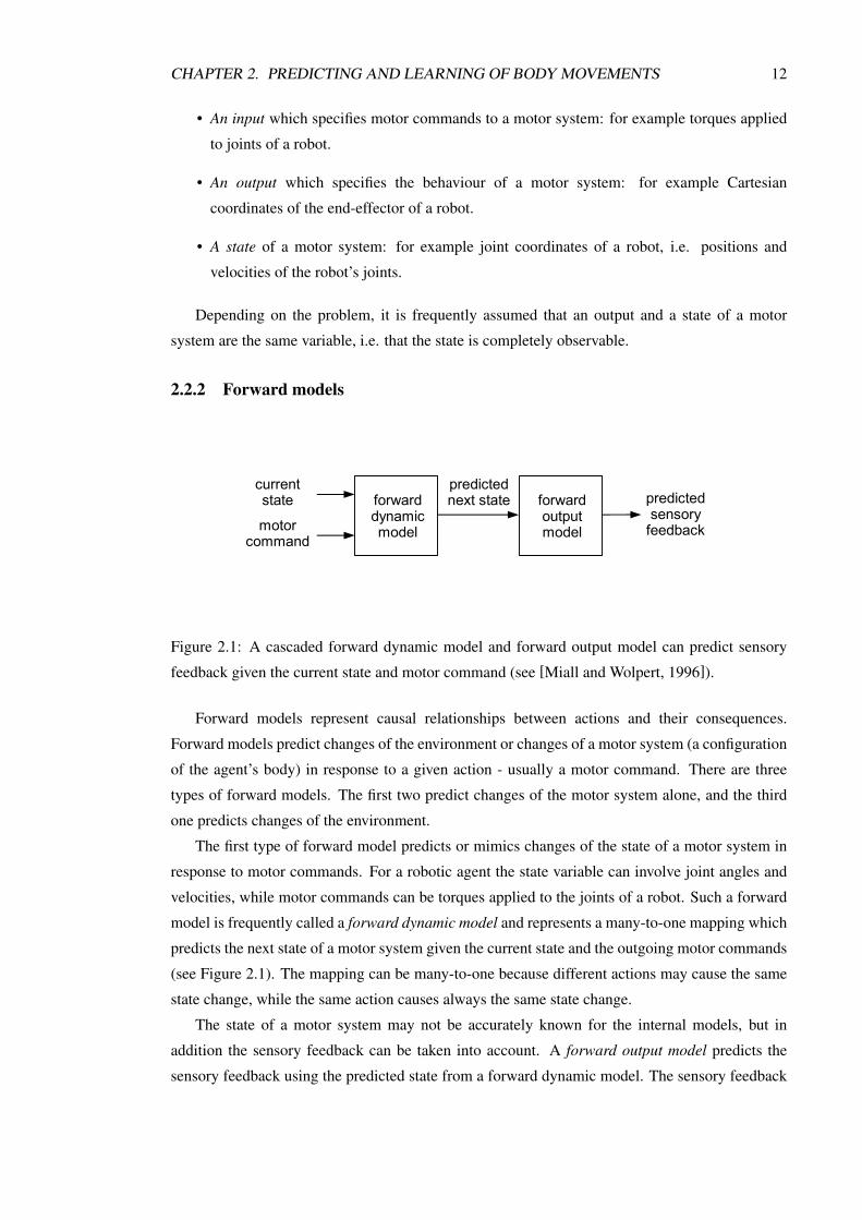
forward dynamic model
predicted sensory
feedback
forward output model
predicted next state
currentstate
motorcommand
Figure 2.1: A cascaded forward dynamic model and forward output model can predict sensory
feedback given the current state and motor command (see [Miall and Wolpert, 1996]).
Forward models represent causal relationships between actions and their consequences.
Forward models predict changes of the environment or changes of a motor system (a configuration
of the agent’s body) in response to a given action - usually a motor command. There are three
types of forward models. The first two predict changes of the motor system alone, and the third
one predicts changes of the environment.
The first type of forward model predicts or mimics changes of the state of a motor system in
response to motor commands. For a robotic agent the state variable can involve joint angles and
velocities, while motor commands can be torques applied to the joints of a robot. Such a forward
model is frequently called a forward dynamic model and represents a many-to-one mapping which
predicts the next state of a motor system given the current state and the outgoing motor commands
(see Figure 2.1). The mapping can be many-to-one because different actions may cause the same
state change, while the same action causes always the same state change.
The state of a motor system may not be accurately known for the internal models, but in
addition the sensory feedback can be taken into account. A forward output model predicts the
sensory feedback using the predicted state from a forward dynamic model. The sensory feedback

CHAPTER 2. PREDICTING AND LEARNING OF BODY MOVEMENTS 13
may involve for example position and velocity of the human arm sensed by muscle spindles or 2D
coordinates of the end-effector of a robot as seen on a video camera image. A cascaded forward
dynamic model and forward output model can predict the sensory feedback given the current state
and motor command (see [Miall and Wolpert, 1996]).
The third type of forward model predicts the behaviour of the external environment due either
to some external cause or to actions of the embedded agent. Exteroceptive senses such as vision or
even touch provide very high dimensional sensory data which are very difficult to interpret because
of the complexity of the physical environment. Building and learning such models remains a
challenge in robotics even in very simple cases. These types of models are discussed in Chapter 3.
2.2.3 Inverse models
forward model
inverse model
desiredoutput
currentstate
motorcommand predicted
sensory feedback
Figure 2.2: Relationship between a forward model and an inverse model. The forward model is a
compound model shown in Figure 2.1.
Inverse models invert the causal flow of the motor commands. Similarly to forward models,
inverse models encapsulate knowledge about the behaviour of a motor system, but instead of
answering a question “what sensory feedback of a motor system causes the given motor command”
they answer “what motor command is required for the desired output of a motor system”. The
input for an inverse model of a robot can be for example the current and the desired spatial pose of
the end-effector, while the output would be a motor command that causes a robotic arm to move
to the desired pose (see Figure 2.2). As forward models represent many-to-one transformations,
inverse models can be one-to-many transformations, i.e. the desired output can be achieved with
many different motor commands. This so-called convexity problem can be avoided by taking into
account additional variables - e.g. the state of a system. The convexity problem is further discussed
in Section 2.5.
2.3 State estimation
The state of a motor system encapsulates all the information which is necessary to control a robot.
The state cannot be sensed directly, however it can be estimated indirectly from a flow of the

CHAPTER 2. PREDICTING AND LEARNING OF BODY MOVEMENTS 14
forward dynamic model
forward output model
next stateestimate
currentstate
estimate
motorcommand
variableKalman
gain
predicted next state
predicted sensory
feedback
sensory
error
actual sensory
feedback
statecorrection
+
+
+-
Figure 2.3: Sensorimotor integration model recursively estimates the state of a motor system by
combining predictions from a dynamical forward model and from a forward output model together
with sensory feedback [Wolpert et al., 1995][Wolpert and Ghahramani, 2000].
input (motor commands) and the output (sensory feedback) of a system. Such a sensorimotor
integration, also known as an observer [Goodwin and Sin, 1984], provides an estimate of the state
integrating motor commands and sensory feedback despite considerable delays caused by the CNS
and time-varying noise and clutter of the feedback.
[Wolpert et al., 1995] investigated target-reaching arm movements in the absence of visual
feedback but in variable conditions affecting proprioception - in null, assistive, or resistive force
fields. Error analysis of the end location of the movements provides a direct support for the
existence of an internal forward model in the CNS which integrates proprioceptive sensations
with motor commands in a similar fashion to the Kalman filter.
The Kalman filter recursively estimates the state of a linear dynamic system from noisy
measurements [Kalman, 1960]. Sensorimotor integration modelled by the Kalman filter
(Figure 2.3) recursively combines two sources of information which together contribute to the
state estimate at the next time step. The first source is the state prediction provided by a forward
dynamic model from the current state estimate and the motor commands. The second source
provides a correction of the state prediction which depends on the sensory error modulated by
the variable Kalman gain. The sensory error is generated by comparing the predicted sensory
feedback from a forward output model with the actual sensory feedback. On the other hand, the
variable Kalman gain depends on the uncertainty of the sensory prediction (as compared to the
uncertainty of the state prediction), so that if the uncertainty is low the sensory prediction mostly
contributes to the state estimate, and vice-versa - if the uncertainty is large the state prediction
takes over the state estimate.

CHAPTER 2. PREDICTING AND LEARNING OF BODY MOVEMENTS 15
2.4 Motor control
The problem of controlling a motor system is directly addressed by the inverse model which
can be seen as a simple controller with a desired behaviour as inputs and corresponding motor
commands as outputs. However robust sensorimotor control in a variable environment requires
incorporating various other factors such as a sensory feedback or the inevitable delays caused by
the finite processing speed of the CNS or any artificial robotic system. Such a control is realized
by a predictive controller introduced further in this section.
2.4.1 Basic control schemes
Following the definitions introduced in Section 2.2.1, we assume that a motor system can be
modelled as a system with:
• Input u which specifies motor commands to a motor system.
• Output y which specifies the behaviour to a motor system.
• State x of a motor system.
The functional relationship between the input, the internal state and the output is many-to-one,
and is described by a forward dynamic model. For discrete time variables t it can be written as
(see Figure 2.4):
yt+1 = h(xt ,ut) (2.1)
A forward model predicts the behaviour of a system yn+1 at the next time step t +1, given current
state xt and motor command ut . Conversely, an inverse mapping between spatial coordinates, joint
coordinates and motor commands is described by an inverse model:
ut = h−1(xt ,yt+1) (2.2)
An inverse model estimates motor command ut required to achieve the desired behaviour of a
system yt+1 at the next time step t +1, given current state xt .
A problem of controlling of a motor system is a problem of achieving the desired behaviour
of its output. In general, there are two classes of controllers [Jordan, 1996][Jordan et al., 1999]:
1. An open-loop feedforward controller which entirely relies on an inverse model of a system
(Figure 2.4)
2. A feedback controller which entirely relies on a feedback from the output of a system
(Figure 2.5)

CHAPTER 2. PREDICTING AND LEARNING OF BODY MOVEMENTS 16
Feedforward Controller
utPlant
yt1* yt
Figure 2.4: A feedforward controller is simply an inverse model of a system (plant). y∗ denotes
the desired output of a system [Jordan et al., 1999].
Feedback Controller
utPlant
yt* yt
Figure 2.5: A feedback controller uses feedback from the output of a system (plant) to correct
control signal u [Jordan et al., 1999].

CHAPTER 2. PREDICTING AND LEARNING OF BODY MOVEMENTS 17
Motor control based on inverse models is referred to as predictive control. Feedforward
controllers guarantee stability of control regardless of noise in the output or the state of a motor
system [Jordan, 1996]. However, feedforward controllers will not maintain the desired output if
the actual state of a motor system diverges from the internal estimate of the state (e.g. because of
any external disturbances), or if the controller itself comprises an inaccurate inverse model of a
system.
2.4.2 Feedback controller
The simplest feedback controller uses the output of a motor system to correct a motor command.
Given desired output y∗ of a system, error-correcting feedback control can be expressed as:
ut = K(y∗t −yt) (2.3)
where K is referred to as a gain, and where for simplicity we assumed that y and u are one-
dimensional vectors. It can be shown that for high values of K, an error-correcting feedback
controller is an equivalent to an open-loop feedforward controller [Jordan, 1996], i.e. the feedback
controller utilizes the implicit inverse of a motor system. In contrast to feedforward controllers,
feedback controllers guarantee maintaining the desired output of a system, however for high values
of K, due to delays and high nonlinearities in the feedback loop, the controlled system may become
unstable.
2.4.3 Composite control system
A composite control system consists of both a feedforward controller and a feedback controller,
so that it combines the best of both worlds (Figure 2.6). The motor command of a composite
controller is a sum of signals from a feedforward controller and a feedback controller:
ut = u f ft +u f b
t (2.4)
If the inverse model is an accurate model of a modelled system and there are no external
disturbances applied to it, motor command u f bt from a feedback controller is negligible. A
composite control signal given by 2.4 is then entirely determined by a feedforward controller.
On the other hand, if the inverse model is inaccurate or there are some external disturbances,
motor command u f bt from a feedback controller drives the system towards desired output y∗1.
2.5 Motor learning
Successful control of a motor system requires an accurate inverse model. In robotics there are well
known classical methods for computing the inverse transformation, using either inverse kinematics
1Assuming that a feedforward controller provides a reasonable estimate of a motor command for desired output y∗.

CHAPTER 2. PREDICTING AND LEARNING OF BODY MOVEMENTS 18
++
Feedback Controller
utPlant
yt1* ytFeedforward
Controller
utff
utfb
Delay
yt*
Figure 2.6: A composite controller consists of both a feedforward controller and a feedback
controller [Jordan et al., 1999]. Delay box stands for a one-time-step time delay.
(global methods) or inverse manipulator Jacobian (local methods) (see Chapter 4). However,
computing the inverse transformation for humanoid robots with 30 or more degrees of freedom2
may be difficult. Furthermore, a fixed inverse model would not allow for specialization in a desired
action domain or for adaptation to variable conditions3. Alternatively, inverse models can be
determined through learning.
2.5.1 Basic learning schemes
Assuming that the desired output of a system is known, the motor learning problem falls into the
domain of supervised learning. For a suitable cost function J, learning becomes an optimization
problem:
J =12‖y∗−y‖2 (2.5)
where y∗ and y are the desired and the actual outputs respectively. A generic supervised learning
system is shown in Figure 2.7.
The simplest method of acquiring an inverse model of the controlled system is called direct
inverse modelling. The idea is to present to a learner various test inputs, observe outputs, and
provide the input-output pairs as a training data, as it is shown on Figure 2.8. The cost function is
defined as
J =12‖ut − ut‖2 (2.6)
where ut denotes the estimated controller input at time t.
2Number of degrees of freedom corresponds to the number of joints and also their type (see Section 4.1).3Such as interaction with a variable environment or a change of the configuration of a body, e.g. due to defects or
growth of a body as in biological systems.

CHAPTER 2. PREDICTING AND LEARNING OF BODY MOVEMENTS 19
+_
Learnerx y
y*
Figure 2.7: A generic supervised learning system [Jordan et al., 1999].
+ _ Feedback Controller
utPlant
yt1
xt
ut
Figure 2.8: The direct inverse modelling approach [Jordan and Rumelhart, 1992]. xt is the
estimated state of the controlled system at time t.

CHAPTER 2. PREDICTING AND LEARNING OF BODY MOVEMENTS 20
Figure 2.9: A learning algorithm averages vectors lying in the non-convex input joint space area
onto a single vector which may lie outside the area (a small circle). Therefore such an averaged
vector may not be an inverse image of the output vector from Cartesian space (a dot). Reprinted
without permission from [Jordan et al., 1999].
Unfortunately, direct inverse modelling has two serious drawbacks[Jordan and Rumelhart,
1992]. Firstly, direct inverse modelling may not converge to correct solutions for such nonlinear
systems such as robotic arms. The problem is referred to as a convexity problem, because of the
non-convexity of areas in the input space (e.g. the joint space of a robotic manipulator), which
correspond to the same values in the output space (e.g. the Cartesian space of the end-effector
of a robotic manipulator). A learning algorithm averages vectors lying in the non-convex input
space area onto a single vector which may lie outside the area. Therefore such an averaged vector
may not be an inverse image of the output vector (Figure 2.9). The one degree of freedom case of
the convexity problem is called “the archery problem” because there can be two angles for which
a projectile reaches a target [Jordan et al., 1999]. Secondly, the method is not goal-directed so
it requires random sampling of the input space. There is no direct way to find some u which
corresponds to a desired output y∗.Feedback error learning is a method of learning a composite control system (Figure 2.10).
The error signal used for learning a feedforward controller is now simply a signal from a feedback
controller u f b. So defined learning error allows the controller to avoid the convexity problem.
This is because instead of averaging in the output space of y, feedback error learning finds a single
solution for a given desired output y∗, due to the fact that feedback error u f b is always greater than
zero in the areas which lie outside of the inverse image (see Figure 2.9).
In contrast to the direct inverse modelling, feedback error learning is goal directed, therefore
it can be used online. Instead of random sampling of the task space, as it is the case in the
direct inverse modelling, feedback error learning can sample the space paired with the output goal
signal y∗t+1. Furthermore, during online learning feedback error u f b from a feedback controller
additionally compensates the difference between the actual behaviour and the desired behaviour.

CHAPTER 2. PREDICTING AND LEARNING OF BODY MOVEMENTS 21
++
Feedback Controller
utPlant
yt1* ytFeedforward
Controller
utff
utfb
Delay
yt*
Figure 2.10: The feedback error learning uses a signal from a feedback controller to learn a
feedforward controller [Jordan et al., 1999].
As an alternative to supervised learning, reinforcement learning algorithms can be used as well
[Jordan et al., 1999]. Reinforcement learning algorithms do not need a performance vector (i.e.
a correct joint signal) for each point in the task space, but only a scalar evaluation. The common
way is to define for each point in the goal space, a set of possible responses together with the
associated probability of selecting each response. If the reward is high, the selection probability is
increased, otherwise the probability is decreased. While reinforcement learning algorithms allow
delayed rewards, they are usually slower than supervised methods.
2.5.2 Learning algorithms
The learning schemes introduced so far are very general, and they do not restrict a learner to any
particular choice. The motor learning problem can be defined as a classification problem, which
involves labelling input patterns, or as a regression problem, which involves finding a functional
relationship between inputs and outputs, i.e. in this case a nonlinear function approximation
with high dimensional input. In further discussion we focus on a regression approach and briefly
present an example method which is widely used in motor learning - the locally weighted projected
regression (LWPR) [Schaal and Atkeson, 1998] [Vijayakumar and Schaal, 2000].
LWPR is an incremental function approximation algorithm which computes prediction y for a
point x (mapping f : x→ y) as a weighted sum of linear models:
y = ∑Mm=1 wmym
∑Mm=1 wm
(2.7)
where all linear models ym are centred at points cm ∈ℜn:
ym = (x− cm)T bm +b0,m = xTmβm (2.8)
where xm = {(x− cm)T ,1}T and βm are the parameters of the locally linear model. The region
of validity of each local linear model, called its receptive field, is determined by weights wm(x)

CHAPTER 2. PREDICTING AND LEARNING OF BODY MOVEMENTS 22
computed from a Gaussian kernel:
wm(x) = exp(−1
2(x− cm)T Dm(x− cm)
)(2.9)
where Dm is a distance metric that determines the size and the shape of region m.
LWPR allows for a convenient allocation of resources, while dealing with the bias-variance
dilemma - a trade-off between over-fitting and over-smoothing. More importantly, since each
local model is learned independently, LWPR directly addresses the negative inference problem - a
problem of forgetting useful knowledge when learning from new data (for details see [Schaal and
Atkeson, 1998]).
2.5.3 Learning movement primitives
While a composite control system (Figure 2.10) can potentially learn an arbitrary movement,
restricting possible classes of movements can reduce the search space during learning and action
recognition. Dynamic movement primitives (DMP) [Ijspeert et al., 2001] [Schaal et al., 2004] are
defined by systems of nonlinear differential equations, whose time evolution naturally smooths
generated trajectories in the kinematic space.
Within the reinforcement learning paradigm, the motor learning problem can be reformulated
as a problem of finding a task specific policy [Peters et al., 2003] [Schaal et al., 2004]:
u = π(y∗,w, t) (2.10)
where y∗ is a desired system state, u is a motor command, and w is an adjustable set of parameters
specific to the policy π (e.g. weights of a neural network). Learning of π quickly becomes
intractable for even a small number of dimensions of the state-action space. However, introducing
prior information about the policy can significantly simplify learning, e.g. in terms of a desired
trajectory.
To increase flexibility, it seems reasonable to provide a set of trajectory primitives rather than
a single desired one. Thus, instead of learning a single policy, a robot can learn a combination of
policy primitives [Schaal et al., 2004]:
u = π(y∗,w, t) =N
∑i=1
πi(y∗,wi, t) (2.11)
On the other hand, it is possible to rewrite the control policy 2.10 as a differential equation [Schaal
et al., 2004]:
y∗ = f (y∗,w, t) (2.12)
the problem of sensorimotor control is then entirely “shifted” to the kinematic space, indepen-
dently of the complex dynamical properties of an entire system. The relationship between kine-
matic variable y and motor command u can then be learned by one of the controllers introduced in

CHAPTER 2. PREDICTING AND LEARNING OF BODY MOVEMENTS 23
++
Feedback Controller
uPlant
y*Movement Primitive
u ff
u fb
Feedforward Controller
y
+
_
Task-specificParameters
Figure 2.11: A composite controller with the dynamic movement primitives (DMP) [Schaal et al.,
2004]. Each DMP can generate trajectories in the kinematic space (the joint space), or alternatively
in the task space (e.g. the Cartesian space).
the previous section independently on the control policy (which does not involve any more the mo-
tor command variable u as in Equation 2.11). A composite controller with the dynamic movement
primitives shown in Figure 2.11, translates a desired kinematic state of the arm y∗, i.e. locations,
velocities and accelerations into torques u. Consequently, complex trajectories in the kinematic
space can be generalized over the entire space, since all the nonlinearities due to dynamics of the
system are accommodated by the controller.
Without delving into unnecessary details, dynamical systems can have two types of attractors4:
a fixed point and a limit cycle. The appropriate sets of differential equations [Ijspeert et al.,
2001] can generate discrete trajectories (discrete DMP) and rhythmic trajectories (rhythmic DMP)
respectively. The shape of trajectories is controlled by a nonlinear function f which can be
conveniently approximated by a locally linear parametric model 2.7 introduced in the section
2.5.2. In addition, rhythmic DMPs can be parametrized by an energy level.
DMPs can be learned in two modes [Schaal et al., 2004]:
Imitation learning. Given the spatiotemporal characteristic of the sample trajectory y, locally
weighted learning (Section 2.5.2) finds the weights of a function estimator of the nonlinear
function f .
Reinforcement learning. The DMP learned by imitation can be further improved with respect
to an optimization criterion. The Natural-Actor Critic (NAC) [Peters et al., 2003] is a
special stochastic gradient method, which injects noise to the control policy in order to
avoid suboptimal solutions. A careful design of control policies can allow a humanoid robot
to play drums or even walk [Schaal et al., 2004].
4We are not dealing here with strange attractors (with fractal structure).

CHAPTER 2. PREDICTING AND LEARNING OF BODY MOVEMENTS 24
The DMPs invariance property also facilitates their further recognition and classification by
using parameters of a function estimator, and e.g. a nearest neighbour classifier.
2.5.4 Modular motor learning
Forward and inverse models introduced so far, are able to capture only one-to-one relation between
motor commands (e.g. torques) and the actual joint configuration of a robot5. For example a single
controller can be trained to perform a particular trajectory for a robotic manipulator. However, the
same controller will generate different trajectory if the hand attached to the manipulator holds a
heavy object. In other words, if the context of a movement changes, the trajectory generated by a
single controller will change as well.
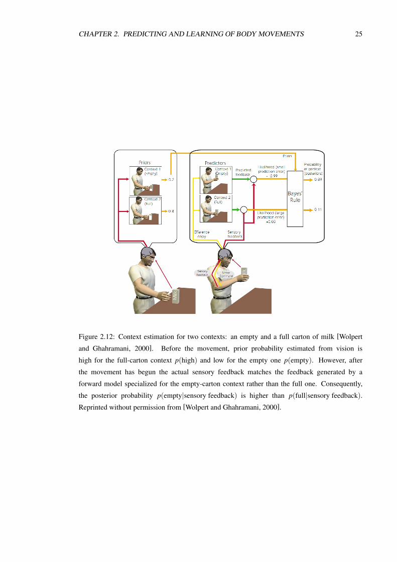
[Wolpert and Ghahramani, 2000] [Wolpert and Kawato, 1998] propose to use context-
specialized controllers and Bayesian approach to estimate the probability of using a particular
context (e.g. whether a hand holds an empty or a full container - see Figure 2.12). According
to Bayes’ theorem, the context posterior probability can be factored into a product of the prior
and the likelihood. The prior p(context) is a probability of a particular context before the
movement, without taking into account the sensory feedback. The prior can be estimated for
example from vision. The likelihood p(sensory feedback|context) is a probability of observing
the current sensory feedback given a particular context. The likelihood can be estimated using a
forward model specialized for a particular context (see Figure 2.12). Bayes’ theorem states that
the posterior probability of a particular context can be estimated as:
p(context|sensory feedback) ∝ p(sensory feedback|context)p(context) (2.13)
The idea of using a Bayesian approach to estimate the context of movements was formalized in
the MOSAIC model [Wolpert and Kawato, 1998] and [Haruno et al., 2001]. The MOSAIC model
splits up experience into multiple internal models which correspond to the movement contexts.
Each internal model consists of a pair of forward and inverse models, so that within each pair a
forward model is learned to predict the behaviour of the associated inverse model (see Figure 2.13).
The system state prediction of the i-th forward model at the next time step t +1 is given by
yit+1 = φ(wi,yt ,ut) (2.14)
where wi are parameters of the model (e.g. weights of a neural network). Assuming that the
system dynamics is disturbed by Gaussian noise with standard deviation σ i, the likelihood of the
i-th context for a given system state yt can be written as [Wolpert and Kawato, 1998]:
lit = p(yt |wi,ut , i) =
1√2π|σ |i)2
exp(−|yt − yi
t |2
2|σ i|2
)(2.15)
5Assuming that there is no perception ambiguity.
CHAPTER 2. PREDICTING AND LEARNING OF BODY MOVEMENTS 25
Figure 2.12: Context estimation for two contexts: an empty and a full carton of milk [Wolpert
and Ghahramani, 2000]. Before the movement, prior probability estimated from vision is
high for the full-carton context p(high) and low for the empty one p(empty). However, after
the movement has begun the actual sensory feedback matches the feedback generated by a
forward model specialized for the empty-carton context rather than the full one. Consequently,
the posterior probability p(empty|sensory feedback) is higher than p(full|sensory feedback).
Reprinted without permission from [Wolpert and Ghahramani, 2000].

CHAPTER 2. PREDICTING AND LEARNING OF BODY MOVEMENTS 26
The responsibility predictor activates modules according to their prior probabilities before any
movement is generated. Prior probability π i of module i is estimated using responsibility predictor
η parametrized by δ i and contextual signal z:
πit = η(δ i
t ,zt) (2.16)
where contextual signal z may involve a target location, an estimate of an object mass, etc.
Figure 2.13: The MOSAIC model consists of N modules [Wolpert and Kawato, 1998], where each
inverse model is associated with a corresponding forward model. Modules are trained according to
their ability to predict the current context (responsibility estimator). Reprinted without permission
from [Wolpert and Kawato, 1998].
Finally, the responsibility estimator activates modules according to their (normalized)
posterior probabilities computed using Bayes’ theorem:
λit =
π it l
it
∑nj=1 π i
t lit
(2.17)
The MOSAIC model can operate in the following modes:
Action production and learning Given contextual signal zt , the responsibility predictor initiates
movement by generating responsibility predictions πt for t ≥ 0. At time t > 0, forward

CHAPTER 2. PREDICTING AND LEARNING OF BODY MOVEMENTS 27
models receive an efference copy of motor commands and produce predicted state yt+1.
The predicted state is then compared to desired state y∗t+1, yielding the prediction error
(y∗t+1− yt+1). In the learning mode, the prediction error is used to learn forward models,
and together with feedback error u f b, to learn inverse models (e.g. in the feedback error
learning scheme introduced earlier in this chapter). The responsibility predictor can be
learnt by comparing responsibility predictions π with posterior probabilities λ .
Action observation During recognition, inverse models produce motor commands which
correspond to the observed action. Although in fact all motor commands are inhibited, their
efference copy is passed to forward models. At time t forward models generate predicted
states yt+1, which are then compared with observed state yt+1 at the next time step t + 1
yielding the prediction error (yt+1− yt+1). The prediction error pattern defines the level of
certainty that a particular action is being demonstrated.
Imitation: Imitation combines action observation followed by action production.
The HMOSAIC model consists of several layers of the MOSAIC model [Wolpert, 2003]. Due
to bidirectional interaction of the lower and the higher modules during learning and control, the
HMOSAIC model can learn how to chunk actions into elementary movements (low level), their
sequences (mid level), and symbolic representation (high level). The inputs of the higher-level
modules are the responsibilities of the lower-level modules, i.e. the higher-level forward models
learn how to predict the posterior probabilities of lower-level models. On the other hand, the
higher-level control models learn the prior probabilities to the lower-level control models, i.e. the
higher-level inverse models generate actions for further elaboration on the lower levels.
The HMOSAIC model is capable of learning progressively both the basic movements at the
lowest level, and their hierarchical temporal order at the higher levels [Wolpert, 2003]. Because
of the tree-like structure the HMOSAIC model can also learn multiple ways to achieve a single
target goal. This is a kind of generalization which enables recognition of the target goal of an
observed action, even though the comparison of the responsibilities of the lower-level modules
may significantly differ.
2.6 Summary
The chapter introduces mathematical models for sensorimotor learning in the context of sensory
prediction. Sensory prediction is thought to be an important mechanism found in many organisms
which facilitates not only perception but also action performance and action learning.
We started with psychological findings supporting the hypothesis that the CNS predicts
sensory consequences of motor actions (Section 2.1). We presented example experiments with eye
and hand tracking. The next Section 2.2 introduces internal models which enable us to control the
relationship between sensory input and motor commands. The forward dynamic model, forward

CHAPTER 2. PREDICTING AND LEARNING OF BODY MOVEMENTS 28
sensory model and inverse model have been also suggested to exists in the cerebellum [Miall and
Wolpert, 1996][Wolpert et al., 1998]. Section 2.3 introduces a sensorimotor integration scheme
for the state of a motor system. It estimates state variables which are required to predict and
control the motor system such as hand or head position. The existence of such state variables has
also been suggested [Goodbody and Husain, 1998].
The later sections introduce mathematical frameworks enabling motor control and learning of
a robot using the hypothesized internal models. Section 2.4 discusses predictive control schemes
which use an inverse model. An inverse model predicts motor commands required to achieve a
desired system behaviour. An inverse model combined with a feedback controller provides an
effective way of controlling robotic systems. Section 2.5 investigates learning of a motor system.
Typically learning of a single controller can be reduced to a regression problem. Significantly
better results can be obtained by constraining the space of possible movements to trajectories
generated by dynamic movement primitives.
Section 2.5.4 introduces modular motor learning which is particularly relevant to this thesis.
Modular motor learning combines several pairs of forward and inverse models where each pair
corresponds to a movement context. Each movement context accounts for a particular situation
which affects a movement, for example for a heavy or light object grasped by a robotic arm. Some
of the problems related to the application of modular motor learning to the pushing experiments
in this thesis are described in more details in the next Chapter 3.
Chapter 3
Predicting object motion duringmanipulation
The previous chapter presented sensorimotor frameworks which enable a robot to successfully
learn and perform movements of the robot’s body, subject to some task goals. Unfortunately,
knowledge of how to move the robots’s own body is not alone sufficient to successfully complete
many simple manipulation tasks such as object pushing or grasping. In particular, because the
manipulated objects are not a part of the robot’s body, forward and inverse models cannot be used
directly without incorporating additional information about the objects’ behaviour.
This chapter introduces the problem of interaction between a robot and the physical
environment in terms of simple pushing manipulation tasks. Despite its seeming simplicity,
pushing manipulation poses several interesting challenges to a robotic learning system. The
chapter also reviews some of the robotics frameworks which have been successfully applied in
the pushing domain and which are relevant to the subject of this thesis.
The contents of this chapter are split into the following sections:
• Section 3.1 introduces prediction learning in robotic pushing manipulation as an important
instance of a problem of interaction learning with the physical world. The section discusses
advantages of learning to predict as opposed to prediction methods which use physics-based
models and do not involve learning.
• Section 3.2 introduces physics-based predictors and discusses some of the problems of
modelling real-word interactions. Physics simulations, although not “biologically inspired”,
can be seen as natural contenders to universal predictors of the physical world.
• Section 3.3 reviews robotic approaches in the pushing manipulation literature. Some of the
approaches address a problem of prediction learning, most notably a problem of affordance
learning. Others make use of prediction during planning of pushing actions. The approaches
in this group have usually limited or no learning capabilities.
29

CHAPTER 3. PREDICTING OBJECT MOTION DURING MANIPULATION 30
• Section 3.4 summarizes the chapter and the challenges posed by the interaction between a
robot body and the physical environment.
3.1 Introduction to prediction learning in pushing manipulation
Pushing manipulation has received comparatively little attention in the robotics research
community. However, pushing operations are encountered very frequently in our everyday
manipulation. They are often connected with grasping in various ways. For example they
frequently precede grasping phase when some parts of the hand touch and move an object before
achieving a stable grasp. During pushing of a heavy object however, grasp may only stabilize a
contact with the object.
For example, in a typical grasping operation, the robot opens a two-jaw gripper wide enough
to accommodate both the workpiece to be grasped and any uncertainty in the workpieces position.
Then the gripper begins to close. Generally the workpiece will be closer initially to one
jaw than to the other, and the closer jaw will make contact first. In general, such situations
result in translation and rotation of the pushed body before the second jaw makes contact, but
particularly severe difficulties are caused by tipping or toppling of the workpiece during grasping
attempts. Furthermore, deliberate manipulation by pushing may often actually be preferable to a
conventional pick and place type operation, especially in cases where the initial and goal positions
of the workpiece share a common support surface. Push manipulation avoids the complexities of
grasping and releasing an object and can greatly extend the manipulation capabilities of robots
which lack the size, strength or grasping hardware, necessary to physically lift an object.
Similarly as in the sensorimotor learning, the ability to predict the movement of an object
in response to a movement of the pusher or equivalently in response to motor commands, is
fundamental to control or planning by a human or by a robot. A prediction problem as discussed in
this thesis is a problem of finding the trajectory of a rigid object given the movement of a pushing
robotic finger and a static ground plane with optional obstacles. Furthermore, we are interested
in learning to predict these trajectories from a number example pushes for various shapes. Apart
from its interesting as a “cognitive way” of solving the prediction problem, prediction learning has
several useful advantages over fixed computation models such as physics simulations:
• It enables adaptation to changing environment conditions without explicit re-estimation of
the model parameters.
• It can improve prediction in the process of learning with arbitrary accuracy, providing that
the learning model is appropriately constructed.
• It provides plausible predictions in situations which are difficult or impossible to model -
for example due to complexity of the physical interactions.
• It provides plausible predictions despite large sensory noise.

CHAPTER 3. PREDICTING OBJECT MOTION DURING MANIPULATION 31
Despite the seeming simplicity of pushing operations, prediction learning of objects’
movements in pushing manipulation is challenging for several reasons:
• Objects may have complex physical properties which are difficult to model. They can have
variable coefficients of friction, restitution, etc. Furthermore, objects themselves do not
have to be rigid.
• Variations in the object shape are potentially infinite and they have a critical influence on
motion.
• The motion of an object depends on surface-surface contacts with other objects. Again,
potential variability here is infinite.
3.2 Physics-based prediction
3.2.1 Physics engines
One of the most obvious ways of predicting the movement of a pushed object is to use physics
laws. Physics-based predictors, in particular physics engines as for example NVIDIA PhysX
[PhysX, 2009] used in some of the experiments in this thesis, predict movements of bodies 1
in response to applied forces or as a consequence of mutual collisions.
Figure 3.1: Bodies in mass-aggregate engines are represented by a set of particles (red circles)
connected by links. The figure shows a character simulation in Twig engine (reprinted without
permission from [Horswill, 2008]).
The mass-aggregate engines represent bodies by a set of mass points or particles connected
by massless rods or links [Millington, 2007]. The body motion can be computed using Verlet
integration [Verlet, 1967]. For example Twig [Horswill, 2008] can simulate characters using a
1Physical objects with a non zero mass.
CHAPTER 3. PREDICTING OBJECT MOTION DURING MANIPULATION 32
mass-aggregate physics engine which is based on Jakobsens work on the Hitman engine [Jakobsen,
2003] (see Figure 3.1). Similar systems of masses connected by springs are also used by NVIDIA
PhysX [PhysX, 2009] to simulate cloths.
The most popular and relevant to this thesis are rigid-body engines. Shapes of the simulated
rigid bodies are represented by geometric primitives such as spheres, cylinders, parallelepipeds,
convex or concave triangle meshes. The body movements are then simple to describe by rigid
body transformations (see Appendix A). Given the initial configuration of the interacting bodies,
the engine subsequently detects all possible collisions as a set of contacts and modifies movement
of the simulated bodies according to one of the contact resolution methods (see Section 3.2.2).
3.2.2 Collisions
Impact occurs when at least two bodies collide with each other within a short period of time. This
causes high levels of forces, high acceleration and deceleration as well as fast energy dissipation.
Impact is closely related to contact which involves a continuous rather than discontinuous process
of two bodies touching each other over a sustained period of time. The difference between impact
and contact corresponds to two major classes of contact resolution methods:
1. Impulse-momentum or discrete methods (Section 3.2.3.1) assume that a single collision
between two bodies does not significantly affect the bodies’ motion during the impact [Kim,
1999]. This assumption limits the approach primarily to rigid bodies. The dynamic analysis
of a single collision can be split then into two parts, where the second part usually resolves
slipping, sticking and reverse motion [Gilardi and Sharf, 2002].
2. Continuous methods or force based methods (Section 3.2.3.2) assume that interaction forces
change in a continuous rather than impulse/discontinuous manner. The bodies’ motion
is resolved by adding and subtracting forces during the contact resolution period. The
methods from this group can offer more realistic approximation of the real behaviour of
the system than discrete methods, in particular in situations which involve more complex
contact configurations [Gilardi and Sharf, 2002].
Contact resolution methods are further discussed in Section 3.2.3.
3.2.2.1 Conservation laws
Two fundamental empirical laws of nature are particularly useful in analysis of collisions between
bodies: conservation of momentum and conservation of energy [Landau and Lifshitz, 1976].
Linear momentum p of a particle with mass m and with linear velocity v is defined as:
p = mv (3.1)

CHAPTER 3. PREDICTING OBJECT MOTION DURING MANIPULATION 33
Angular momentum L of a particle with linear momentum p which moves in a reference frame
with radial vector r is defined as:
L = p× r (3.2)
Alternatively, a body rotating around fixed axis with angular velocity ω and inertia tensor I(represented by 3×3 real matrix) has angular momentum given by:
L = Iω (3.3)
The law of conservation of momentum states that the sums of linear momentum and angular
momentum of all bodies of a closed system are constant, i.e.
∑i
pi = const (3.4a)
∑i
Li = const (3.4b)
Consequently, momentum of a particular body can be exchanged with other bodies, but the total
momentum of the system of bodies is always preserved.
The law of conservation of energy states that the total amount of energy of a closed system
remains constant over time. Although, the total energy of a system of colliding bodies is preserved,
it can change their form from the kinetic energy into plastic deformation of bodies or into heat and
sound in energy dissipation process. The energy loss El caused by impact can be approximated by
negative work done by contact force Fc during the collision [Stronge, 1992]:
El =−∫
Fc · δdt =−∫
Fcdδ (3.5)
where time-dependent variable δ models the body surface deformation. From the law of
conservation of energy we have:
E1k = E2
k −El (3.6)
where E1k and E2
k are kinetic energy of the bodies before and after the collision. If El = 0 the
collision is perfectly elastic, if E2k = 0 the collision is perfectly plastic.
The energy loss is directly related with the phenomenon of wave propagation within colliding
bodies. Because bodies are not perfectly rigid, stress caused by the body deformation propagates
with a finite velocity, this in turn results in oscillations. Details of this process are studied in
[Stronge, 2004].

CHAPTER 3. PREDICTING OBJECT MOTION DURING MANIPULATION 34
time
deformation
A
Ocompression restitution
B
C D
Figure 3.2: Body deformation during impact consists of compression and restitution phases (see
[Gilardi and Sharf, 2002]).
3.2.2.2 Restitution
The body deformation during impact depends on many physical properties such as material, shape
or approach velocity. Nevertheless one can distinguish two deformation phases: compression and
restitution [Gilardi and Sharf, 2002]. The compression phase begins when two bodies first make
contact at point O on the time-deformation diagram in Figure 3.2, and finishes at point A of the
maximum deformation of a body. The restitution phase starts at point A and it can finish on the
same point A (perfectly plastic collision), point B (partially plastic collision), point C (perfectly
elastic collision with no energy loss) or point D (partially elastic collision with energy loss but no
permanent deformation).
The body deformation caused by impact is very difficult to model, however the impact energy
loss El can be conveniently approximated by a coefficient of restitution e such that 0 ≤ e ≤ 1. If
the collision is perfectly elastic then e = 1, for a perfectly plastic collision e = 0.
There have been proposed several definitions of the coefficient of restitution. For example,
Newton model is discussed in [Whittaker and McCrea, 1988], Poisson model [Routh, 1905] or
Stronge model [Stronge, 2004].
3.2.2.3 Friction
Friction is another key aspect of impact and contact dynamics, it causes energy dissipation and
may stop or even reverse the body movement. Coulomb’s law is the most widely used model of
friction due to its simplicity and good approximation accuracy [Mason, 2001].
Consider a solid block on the table as in Figure 3.3 with clean, dry and unlubricated surfaces.
A slowly rising force Fa is applied to the block with the gravity force Fn = mg normal to the
surface. The tangential force Ft prevents the block from movement until Fa reaches level Fts. The
motion begins and Fa decreases to Ftd . Fts and Ftd can be approximated by

CHAPTER 3. PREDICTING OBJECT MOTION DURING MANIPULATION 35
F a
F t
F t F a
F n
s F nd Fn
Figure 3.3: Coulomb’s law of sliding friction describes the body motion using the static coefficient
of friction µs and the dynamic coefficient of friction µd .
Fts = µsFn (3.7)
Ftd = µdFn (3.8)
where µs is the static coefficient of friction and µd the dynamic coefficient of friction. Two
situations are possible:
1. Sticking if there is no motion |Fa| ≤ µs|Fn|.
2. Sliding when |Fa|= µd |Fn|
The main problem with Coulomb’s law is the discontinuity of the tangential force due to static
and dynamic behaviour. A non-local model of friction [Oden and Pires, 1983] relates a value
of friction at one point to values of friction in the point neighbourhood. A non-linear friction
model allows a continuous transition from the sticking phase to the sliding phase [Haessig Jr and
Friedland, 1991] [Oden and Pires, 1983].
3.2.3 Contact resolution methods
3.2.3.1 Discrete methods
The discrete methods assume that impact between bodies is instantaneous and results in impulse
forces and discontinuous changes of the kinematic variables (velocities) but without instantaneous
displacements of the interacting bodies. The model usually assumes that colliding bodies are rigid
and all the bodies’ deformations can be approximated using coefficients of restitution and friction.
The collision problem can be solved using the law of conservation of momentum 3.4b called
impulsemomentum principle for collisions. The time integral of the contact force Fc is called

CHAPTER 3. PREDICTING OBJECT MOTION DURING MANIPULATION 36
impulse. Linear impulse P represents a change of the body momentum between t1 and t2 caused
by force Fc:
P =∫ t2
t1Fc(t)dt (3.9)
If p is the momentum of the colliding body, r is the distance from the centre of the mass to the
point of impact, L is the angular momentum, P and M are the linear and angular impulses, then
the relations between these variables before the impact at time t1 and after the impact at t2 for two
colliding bodies, specified with subscripts 1 and 2, can be expressed by [Brach, 2007][Gilardi and
Sharf, 2002]:
pt21 −pt1
1 = P (3.10a)
pt22 −pt1
2 =−P (3.10b)
Lt21 −Lt1
1 = r1×P+M (3.10c)
Lt22 −Lt1
2 = r2×P−M (3.10d)
where the change of linear and angular velocities as well as the linear and angular impulses have
to be computed. In order to solve the above equations additional relations must be provided. In
many approaches the angular impulse M is neglected. The motion of the body at the contact
can be decomposed into normal and tangential directions, so the kinematic constraints involving
coefficients of restitution and friction can be applied (for details see [Gilardi and Sharf, 2002]).
Applications of restitution and friction models (Sections 3.2.2.2 and 3.2.2.3) in many situations
may violate the law of energy conservation during the frictional impact2. The inconsistent results
are consequence of the definition of coefficients of restitution and may result in possible changes
of slipping direction or overestimation of the final velocity after the impact [Stronge, 1991]. To
account for these inconsistencies [Stronge, 1992] proposed the coefficients of restitution and
friction to be independent. [Brach, 2007] introduced energy and kinematics constraints on the
impulse ratio which describe the body behaviour in tangential directions
Furthermore, some of the inconsistencies arise due to the discontinuities in Coulomb’s law of
friction, so that no or multiple solutions may exist. Alternative models have also been proposed
(see Section 3.2.2.3), however no optimal solution has been found yet [Gilardi and Sharf, 2002].
Another problem is related to the basic assumption of the model: the objects’ rigidity and
vanishingly short duration of impacts. Bodies can have multiple contacts and the order of resolving
them can yield different results [Stronge, 2004].
3.2.3.2 Continuous methods
Continuous models, also referred to as compliant contact models, overcome some of the
weaknesses of the discrete methods [Gilardi and Sharf, 2002]. Unlike the discrete methods, the2I.e. involving friction.

CHAPTER 3. PREDICTING OBJECT MOTION DURING MANIPULATION 37
continuous models explicitly account for the deformations caused by the forces during impact.
A large class of continuous models, the explicit models, relate the contact normal force Fn as an
explicit function of the local surface indentation δ [Brach, 2007]:
Fn ≡ Fn(δ , δ ) = Fδ (δ )+Fδ(δ ) (3.11)
Several models have been proposed to approximate force Fn. Hertz’s model ([Hertz, 1896])
assumes elastic deformations and originally does not include damping:
Fn = kδm (3.12)
where k and m are material and geometry-specific constants. The model has been later extended
to plastic deformations in [Abrate, 1998]. [Goldsmith, 1960] introduced spring-dashpot model
represented by a linear damper to account for energy dissipation with force Fn approximated as:
Fn = kδ +bδ (3.13)
A more physically realistic model introduced in [Hunt and Crossley, 1975] combines advantages
of the Hertz’s model and the spring-dashpot model. The model includes a non-linear damping
term into the contact normal force Fn formula:
Fn = bδpδ
q + kδm (3.14)
Furthermore, as shown in [Hunt and Crossley, 1975] damping coefficients can be related with the
coefficients of restitution.
There are two major groups of methods with respect to the type of equations of motion for
the colliding bodies (for details see [Gilardi and Sharf, 2002]). Methods in the first group solve
an explicit functional relationship between the contact force and the generalized coordinates3,
including dependencies on material properties and other geometric properties. The second group
of methods takes into account the surface deformation due to collision using flexibility properties
of the contacting bodies, however without employing the surface normal forces.
Continuous methods have important advantages over discrete methods. They do not need to
distinguish between impact and contact situations and naturally extend to situations with multiple
bodies and contacts [Gilardi and Sharf, 2002]. Furthermore they allow for using any friction
model, including the models described in Section 3.2.2.3.
Continuous methods employing a non-linear damping term can model the real behaviour of
the system quite well, however the appropriate parameters of the model can be difficult to obtain
in practice.
3Positions and velocities.

CHAPTER 3. PREDICTING OBJECT MOTION DURING MANIPULATION 38
3.3 Pushing manipulation in literature
3.3.1 Pushing and planning
A majority of engineering literature which addresses the problems of robotic manipulation by
pushing, focuses on planning and relies on physics-based prediction of simple 2D shapes sliding
over a flat 2D surfaces. Fundamental work in this field comes from Mason [Mason, 1982][Mason
and Salisbury, 1985][Mason, 1986] who was one of the first to identify pushing operations as
fundamental in manipulation, and especially in grasping. Mason developed a detailed analysis of
the mechanics of pushed, sliding objects and determines conditions, in terms of centre of friction,
centre of gravity, point of application and direction of motion of an applied force from a position
controlled pusher, required for translation, clockwise rotation and counter-clockwise rotation of a
pushed object. The work can be considered “qualitative” in that exact conditions are found which
can determine which of various qualitatively different behaviours of the pushed object will occur.
Masons work was extended by Peshkin and Sanderson [Peshkin and Sanderson, 1985], [Peshkin
and Sanderson, 1986], [Peshkin and Sanderson, 1988], who attempt to put quantitative bounds on
the rate at which these predicted motions occur. This rate information is important for planning
guaranteed manipulation strategies. This work also built on ideas from the automation community,
where pushing operations had long been a familiar tool for orienting components travelling on a
factory conveyor belt, by using systems of fences, e.g. [Mani and Wilson, 1985].
Later work proposed methods of path planning for push manipulation of 2D objects. The
behaviour of the workpiece during grasping is discussed by Brost [Brost, 1988], who finds grasp
strategies which bring the workpiece into a unique orientation in the gripper, despite substantial
uncertainty in its initial orientation and position. Lynch [Lynch, 1992] developed a method for
finding the set of all possible motions of a sliding object, in response to an applied push. Using
this information it is possible to find the set of pusher motions which maintain a particular pusher-
slider contact configuration. Such motions may be continued indefinitely and can be used for
planar parts transfer operations, comprising what Lynch terms a stable non-grasp. More recently,
Cappelleri [Cappelleri et al., 2006] has developed path planning techniques for push manipulation
of 2D sliding objects. Cappelleri has examined push manipulation of millimetre scale objects
with a manipulated needle. He solves a millimetre scale 2D version of the classic peg in the hole
problem, using physics simulations to predict the workpiece movements which will result from
applied robot push primitives, and then planning a sequence of such pushes to achieve an end
goal state, using a modified Rapidly Exploring Random Tree (RRT) algorithm. Other work on 2D
manipulation by pushing includes the use of a mobile robot vehicle to push objects around a floor
space [Yoshikawa and Kurisu, 1991].
In contrast, we know of comparatively little literature which addresses the more complex
problems of predicting the results of push manipulations on real 3D bodies, which are free to
tip or roll, as well as perform simple translation and rotation under sliding. This problem is further

CHAPTER 3. PREDICTING OBJECT MOTION DURING MANIPULATION 39
compounded by the fact that real 3D objects will behave in very different ways depending on their
poses relative to both the manipulator and the surface on which they rest. Hence, models of the
workpieces dynamics, kinematics, friction parameters etc. which are learned in one configuration
may be completely unusable once, for example, the object has toppled over into another pose
relative to the tabletop.
3.3.2 Learning
Metta [Metta and Fitzpatrick, 2003], use a robot arm to push various parts of the environment,
in order to aid a vision system in identifying which parts of a scene comprise distinct objects,
according to a criterion of consistent regions of optic flow. However, this work does not attempt
to learn how to predict the the motions that will result from such pushes. Robotic systems have
been developed to learn pre-specified binary affordance classes, e.g. rolling versus non-rolling
objects [Fitzpatrick et al., 2003] or liftable versus non-liftable objects [Paletta et al., 2007].
Ridge [Ridge et al., 2008] present experiments where a robot arm coupled to a vision system
learns affordances of various different objects by applying pushes and then observing the resulting
motions. The system performs simple push actions on everyday objects (e.g. a pepsi can and a
mobile phone) that are placed on a work surface. The vision system extracts the resulting motion
of the pushed objects and gathers features such as mean velocity, total distance travelled and
final object orientations. These features, with the associated object label, are used to train a self
organizing map, thereby learning to distinguish between objects that roll (e.g. Pepsi can) and those
that do not (e.g. mobile phone).
This kind of approach is limited, in that affordances learned for a specific object and push
action, may not be generalizable to a new object or even the same object but in a different
orientation or subjected to a different kind of push. Furthermore, although certain primitive classes
of motion, e.g. rolling, may be predicted, such systems cannot predict the explicit rigid body
motion that will result when an object is subjected to a push, and are thus of limited value for
either planning or control during push manipulation operations.
3.4 Summary
This chapter introduced pushing manipulation as an important aspect of interaction of a robot
with the physical environment. In particular it focused on prediction of the motion of an object
subjected to a pushing movement of a robotic manipulator. This kind of prediction is performed
by physics simulators, which indeed are used as predictors in robotic scenarios. As it is argued in
Section 3.1, learning to predict may offer several benefits over prediction performed by fixed
models4 which may not be able to match reality in situations where accurate predictions are
essential (e.g. during planning) or when only noisy sensory data is available.
4I.e. models which explicitly encode some aspects of physics, despite tuning the parameters of a model.
CHAPTER 3. PREDICTING OBJECT MOTION DURING MANIPULATION 40
Section 3.2 is a brief introduction to physics engines. Physics engines represent objects usually
as geometric primitives and predicts their motion in terms of rigid body transformations using laws
of physics. They subsequently detect all collisions as sets of contacts and modify the movement
of simulated bodies using contact resolution methods. Unfortunately, none of these methods are
without drawbacks. Friction and restitution are particularly difficult to model, and frequently
lead to situations which violate the law of energy conservation. Furthermore, the order in which
contacts are resolved is critical and have great influence on the predicted motion. On the other
hand, continuous methods are relatively insensitive to the contact resolution order since they
explicitly handle deformations during a single contact. These models, however, are expensive
and appropriate parameters of the model can be difficult to obtain in practice.
Section 3.3 presented a literature review on pushing manipulation in robotics which can be
split into two major groups. Approaches from the first group are focused on planning, usually
employing physics-based forward models. Most of the approaches from this group is also limited
to 2D simplified world. Approaches from the second group enable learning of the objects’
behaviour, however they are mostly focused on the preprogrammed qualitative behaviour of
objects during pushing and poking actions.

Chapter 4
Controlling a robotic manipulator
One of the most important problems of control and movement planning for a robotic manipulator,
is the problem of finding motor commands such that the manipulator body follows a desired
trajectory. This control problem could be addressed by some of the sensorimotor learning
approaches presented in Chapter 2. However, the algorithms described in this chapter take a
classical path planning approach rather than a learning approach to this motion control problem.
One of the reasons for abandoning the learning approaches in this context, is that they do not
provide sufficiently simple and flexible ways to handle constraints which in practice have to be
imposed on-line on the motion of a manipulator in the presence of obstacles1 This approach also
allows us to focus on the prediction learning problem independently of learning control.
The algorithms presented in this chapter are suitable for any open-chain robotic manipulator
with position control, such as the Katana 6M180 [Neuronics AG, 2004] - a robotic manipulator
which has been used in the most of the robotic experiments in this thesis. The algorithms have
been implemented as part of the control software framework and they entirely replaced the original
manufacturer’s Katana control software2.
Although, the presented algorithms are mostly based on the state-of-art algorithms for the
manipulator control and path planning, there are a few minor contributions which are described in
the final section of this chapter.
The chapter consists of the following sections:
• Section 4.1 briefly describes the design of typical robotic manipulators, introducing some
basic concepts such as the number of degree of freedom, joint types, the joint space and the
workspace of a manipulator.
1The robotic manipulator used in the pushing experiments, the Katana 6M180 [Neuronics AG, 2004], is a purely
position controlled manipulator without any compliance capabilities or motor current limitation features. Consequently,
any position error during movement execution, in the presence of a table, may immediately cause serious damage to
the manipulator.2Katana Native Interface only allows for movements by specifying the movement end-point computed by the build-
in inverse kinematic module. It does not allow for any trajectory or path control between the start point and the end
point of a movement.
41

CHAPTER 4. CONTROLLING A ROBOTIC MANIPULATOR 42
• Section 4.2 contains a derivation of formulas for the forward kinematics and the forward
instantaneous kinematics using the notation introduced in Appendix A. The section
discusses methods of solving the inverse kinematics problem and the inverse instantaneous
kinematics problem which are required by the motion control algorithms.
• Section 4.3 introduces the problem of controlling the motion of a robotic manipulator given
the desired trajectory in the joint space or the workspace of a robotic manipulator.
• Section 4.4 discusses the problem of planning trajectories of the manipulator body in
the presence of other bodies, and presents methods for collision detection during path
and trajectory planning. The section also describes a trajectory planner used in pushing
experiments from this thesis, which combines the trajectory planner together with a
capability to change the movement plan online, i.e. during its execution.
• Section 4.5 summarizes the movement planning methods used by the Golem framework and
in the experiments in this thesis.
4.1 Robot design
A typical robotic manipulator (also called a robotic arm) consists of a set of rigid links
interconnected by joints. If the links are connected serially, one after the other, a robotic
manipulator is called then an open-chain robotic manipulator. Joints are usually actuated by
motors (although passive joints can also be used), so that a whole manipulator can be controlled to
perform given tasks. A tool or end-effector, usually a gripper, is attached at the end of the chain of
links. The Katana 6M180 robotic arm is an example of an open-chain manipulator with a simple
gripper with two fingers as shown in Figure 4.1.
In classical mechanics the degree of freedom (DOF) is the number of independent variables
which must be specified to uniquely determine the position of a system. A rigid body in a 3D
Euclidean space requires at least 6 numbers to uniquely specify its pose or configuration, i.e the
position and orientation of the body (see Appendix A). In the case of a robotic manipulator the
number of degree of freedom or degree of mobility refers to a number of independent variables
which uniquely determine the position of each joint of the manipulator (usually excluding a
gripper). Therefore the number of DOF depends on a number of joints as well as on their type.
4.1.1 Manipulator joints
There are several joint types which are used in robotic manipulators. However four of them are
the most frequently used: revolute, prismatic, cylindrical and spherical.
A revolute joint is by far the most common type of joint used in robotics (see left top panel
in Figure 4.2). It is a 1-DOF joint, which means that there is one number required to uniquely

CHAPTER 4. CONTROLLING A ROBOTIC MANIPULATOR 43
Figure 4.1: The Katana 6M180 robotic manipulator is a 5-DOF manipulator consisting of 5 joints
([Neuronics AG, 2004]). The Katana manipulator also has a gripper with two fingers mounted at
the end-effector.
specify its configuration - a rotation angle around a fixed axis. The Katana manipulator is built of
5 such joints.
A prismatic joint is another commonly used joint. It has 1-DOF which corresponds to a pure
translational movement along a fixed axis (see right top panel in Figure 4.2).
A cylindrical joint has 2-DOF which correspond to translational movement along a fixed axis
and rotational movement around the same axis (see left bottom panel in Figure 4.2). This kind of
joint is usually built as a combination of a prismatic joint and revolute joint.
A spherical joint has 3-DOF and is capable of arbitrary rotations around a fixed point (see
right bottom panel in Figure 4.2). Spherical joints are usually built as a combination of 3 revolute
joints such that their axes of rotation intersect at a single point. In this way the orientation of a
joint can be uniquely parametrized by three angles.
All variables parametrizing the configuration of an arbitrary joint will be further referred as to

CHAPTER 4. CONTROLLING A ROBOTIC MANIPULATOR 44
Figure 4.2: 4 most frequently used joint types: 1-DOF revolute joint (left top panel), 1-DOF
prismatic joint (right top panel), 2-DOF cylindrical joint (left bottom panel) and 3-DOF spherical
joint (right bottom panel).
joint variables.
4.1.2 Manipulator configuration space
The configuration of each manipulator joint i is determined by a corresponding joint variable θi.
Interestingly, all joints with 2 or more DOF, as for example cylindrical joints or spherical joints
(Section 4.1.1), can be represented as a combination of 1-DOF revolute joints and prismatic joints
[Murray et al., 1994].
Joint variables parametrizing manipulator joints are limited to the intervals θi ∈ [ai,bi] ⊂ R,
where a particular choice of ai and bi depends on the manipulator design. For a revolute
joint the (half-open) interval is naturally associated with a unit circle in the plane S1 such that
0 < bi−ai ≤ 2π .
The set of all joint variables constitutes the joint space C (more generally the configuration
space) of a manipulator. The joint space of a manipulator consisting of p revolute joints
and r prismatic joints is defined as a Cartesian product of p unit circles and r intervals C =
S× . . .×S×R× . . .×R = Tp×Rr, where Tp is a p-torus and Rr is a r-cube. For example the
joint space of the 5-DOF Katana manipulator is a 5-torus C = T5.
An element θ ∈ C is called the manipulator configuration. The reference configuration of a
manipulator is defined as a configuration which corresponds to θi = 0 for all joint variables. A
particular choice of the reference configuration is arbitrary, however to simplify calculations it is
usually assumed that the manipulator is “stretched” along one of the coordinate axes of the base
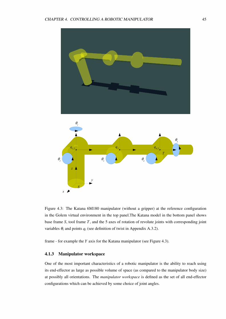
CHAPTER 4. CONTROLLING A ROBOTIC MANIPULATOR 45
x
y
z
S
T
θ1
θ2
θ3
θ4
θ5
q1,2 q3 q4,5
Figure 4.3: The Katana 6M180 manipulator (without a gripper) at the reference configuration
in the Golem virtual environment in the top panel.The Katana model in the bottom panel shows
base frame S, tool frame T , and the 5 axes of rotation of revolute joints with corresponding joint
variables θi and points qi (see definition of twist in Appendix A.3.2).
frame - for example the Y axis for the Katana manipulator (see Figure 4.3).
4.1.3 Manipulator workspace
One of the most important characteristics of a robotic manipulator is the ability to reach using
its end-effector as large as possible volume of space (as compared to the manipulator body size)
at possibly all orientations. The manipulator workspace is defined as the set of all end-effector
configurations which can be achieved by some choice of joint angles.

CHAPTER 4. CONTROLLING A ROBOTIC MANIPULATOR 46
Two subspaces of the manipulator workspace can be considered:
• The reachable workspace is the set of all positions which can be reached by some choice of
joint angles irrespectively to the end-effector orientation.
• The dexterous workspace is the set of all positions which can be reached by some choice of
joint angles and for an arbitrary orientation of the end-effector.
It is clear that manipulators which have less than 6 DOF cannot have the dexterous workspace
(of volume larger than zero). This is because there are (almost) no end-effector configurations
for which there can be found a corresponding set of joint angles. An example of such a robotic
manipulator is the Katana 6M180 which has 5 DOF.
4.2 Robot kinematics
The kinematics of a robotic manipulator describes the relationship between the joint variables and
the configuration of the parts of a robot body, in particular the configuration of the end-effector of
a robot. There can be two kinds of relations considered:
1. A many-to-one mapping between the joint variables and the configuration of the robot end-
effector. The problem of finding this mapping is called the forward kinematics problem if it
involves joint positions, or the forward instantaneous kinematics problem if it involves the
joint velocities and the velocity of the robot’s end-effector. Solutions to these problems can
be always found analytically for any set of joint variables.
2. A one-to-many relation between the configuration of the robot end-effector and the joint
variables. The problem of finding joint positions for a given configuration of the end-
effector is called the inverse kinematics problem. The problem of finding joint velocities for
a given velocity of the end-effector is called the inverse instantaneous kinematics problem.
The exact solutions to these problems may not exist, however it is always possible to find
approximate solutions.
A formal derivation of formulas for the forward kinematics and the forward instantaneous
kinematics is contained in Sections 4.2.1 and 4.2.2.
The problem of finding joint positions and velocities for a given end-effector configuration
and velocity is of particular importance for the motion control of a robotic manipulator (see
Section 4.3). A simple point-to-point motion of a manipulator requires at least computing joint
positions which correspond to the final desired configuration of the end-effector. This problem can
be solved using inverse kinematics algorithms described in Section 4.2.3. A more general case can
involve intermediate points on a trajectory with specified configurations of the end-effector as well
as its velocity - the linear and the angular velocity of the end-effector. This problem is addressed
in Section 4.2.4.

CHAPTER 4. CONTROLLING A ROBOTIC MANIPULATOR 47
4.2.1 Forward kinematics
Consider a model of the Katana manipulator as an example of an open-chain robotic manipulator
(see Figure 4.3). One can attach a reference frame to each link of the manipulator. In particular, the
base frame S is attached to the first immovable link, for example at the bottom of the manipulator.
The tool frame T is attached to the last link of the manipulator, i.e. to its end-effector.
The forward kinematics problem is a problem of finding the configuration of the tool frame T
given a set of joint variables θ ∈ C of a particular robotic manipulator. The forward kinematics is
represented by mapping gst : C → SE(3) which determines a rigid body transformation between
the tool frame T and the base frame S. The forward kinematics can be conveniently represented
as a product of exponentials of twists corresponding to the each joint of a manipulator ([Murray et
al., 1994]).
The transformation eξ θ associated with twist ξ (see introduction in Appendix A) moves frame
B from its initial configuration gab(0) in the frame A to the final configuration gab(θ) as below
(see Equation A.61):
gab(θ) = eξ θ gab(0) (4.1)
Twist ξ can represent any rigid body transformation including motion generated by a joint between
frames A and B attached to its two adjacent links, with θ corresponding to the amount of rotation
for a revolute joint or to the amount of translation for a prismatic joint.
Following Equation A.46, the rotational motion of a revolute joint i around axis ωi ∈ R3 with
any point qi ∈ R3 on the axis is represented by twist ξi with twist coordinates:
ξi =
[−ωi×qi
ωi
](4.2)
The cross product used in the above expressions allows for an arbitrary choice of a point qi on
the axis ωi. For example, for the Katana manipulator, point q1 corresponding to twist ξ1 can
lie anywhere on Z axis of the local reference frame, while point q2 corresponding to twist ξ2
anywhere on X axis. For convenience they both are chosen to lie at the origin the same frame (see
Figure 4.3).
Furthermore, following Equation A.53, the translational motion of a prismatic joint i in the
direction pointed by vi ∈ R3 is represented by twist ξi with twist coordinates:
ξi =
[vi
0
](4.3)
Consider the Katana manipulator at the reference configuration for which all joints apart from
the last one have been fixed at zero position so that θ1 = 0,θ2 = 0,θ3 = 0,θ4 = 0 with variable θ5
(Figure 4.3). From Equation 4.1 follows that the rigid motion associated with twist ξ5 and θ5 can
be written as:

CHAPTER 4. CONTROLLING A ROBOTIC MANIPULATOR 48
gst(θ5) = eξ5θ5gst(0) (4.4)
where twist coordinates ξ5 are constructed as in Equation 4.2 and where gst(0) represents the rigid
body transformation between tool frame T and base frame S at the reference configuration. After
applying a movement, let the last joint 5 be fixed and move only joint 4 with associated twist ξ4
and joint variable θ4. The end-effector configuration becomes:
gst(θ4,θ5) = eξ4θ4gst(θ5) = eξ4θ4eξ5θ5gst(0) (4.5)
Repeating the above procedure for all the other joints gives a formula for the manipulator
forward kinematics. It turns out that the above procedure is also independent on the order in
which the movements are applied to joints ([Murray et al., 1994]).
Applying a movement first to joint 4 is simple and gives:
gst(θ4) = eξ4θ4gst(0) (4.6)
Moving joint 5 is not so straightforward because the movement of joint 4 has already changed the
rotation axis ω5 of joint 5 and consequently the twist coordinates ξ5. Applying movements to each
joint in descending order as before allows us to avoid this situation.
For a given g ∈ SE(3) one can introduce Adg - a 6×6 matrix called the adjoint transformation
(see A.88):
Adg =
[R pR
0 R
](4.7)
Then the changes of the twist coordinates ξ5 for transformation eξ4θ4 can be represented as follows:
ξ′5 = Ad
eξ4θ4ξ5 (4.8)
The corresponding twist ξ ′5 transforms according to Equation A.84, so that the transformation
generated by ξ ′5 and θ5 is given by:
eξ ′5θ5 = eeξ4θ4 (ξ5θ5)e−ξ4θ4 = eξ4θ4eξ5θ5e−ξ4θ4 (4.9)
where in the last step identity A.94 has been used. The combined transformation is:
gst(θ5,θ5) = eξ ′5θ5eξ4θ4gst(0) = eξ4θ4eξ5θ5e−ξ4θ4eξ4θ4gst(0) = eξ4θ4eξ5θ5gst(0) (4.10)
which is the same as Equation 4.5.
The above procedure can be generalized to arbitrary number of joints n with joint variable
θ = (θ1, . . . ,θn)∈C = Rn. The forward kinematics gst : C → SE(3) of an open-chain manipulator
can be written as:

CHAPTER 4. CONTROLLING A ROBOTIC MANIPULATOR 49
gst(θ) = eξ1θ1eξ2θ2 . . .eξnθngst(0) (4.11)
The major advantage of forward kinematics in the above form as compared to e.g. Denavid-
Hartenberg parameters ([Denavit and Hartenberg, 1955]) is its simplicity. Creation of the forward
kinematics map comes down to specifying twists coordinates ξi for each joint i in terms of axes
of rotation ωi or directions of translation vi and their spatial locations - points qi (see for example
Katana manipulator on Figure 4.3). Rigid body transformation gst for a particular joint variable
vector θ is then obtained as a product of exponentials of matrices ξiθi using formulas A.56 and
A.57.
4.2.2 Forward instantaneous kinematics
The forward instantaneous kinematics problem for an open-chain manipulator addresses the
problem of finding the end-effector velocity, given the positions and the velocities of the
manipulator joints.
The end-effector velocity can be expressed in terms of the instantaneous spatial velocity of a
rigid body introduced in Section A.4. From Equation A.76 it follows that the instantaneous spatial
velocity of the end-effector is given by a twist:
V sst = gst(θ)g−1
st (θ) (4.12)
where gst(θ) is the manipulator forward kinematics 4.11. gst(θ) depends on joint variable vector
θ ∈Rn which changes in time as the manipulator moves along a trajectory θ(t). Therefore a chain
rule can be applied to gst(θ), so that Equation 4.12 becomes:
V sst =
n
∑i=1
(∂gst
∂θiθi
)g−1
st (θ) =n
∑i=1
(∂gst
∂θig−1
st (θ))
θi (4.13)
Because V sst is a twist, Equation 4.13 can be rewritten in twist coordinates:
V sst = Js
st(θ)θ (4.14)
where Jsst(θ) is a 6×n matrix called the spatial manipulator Jacobian ([Murray et al., 1994]):
Jsst(θ) =
[(∂gst
∂θ1g−1
st
)∨. . .
(∂gst
∂θng−1
st
)∨]=[ξ′1 . . .ξ ′n
](4.15)
where the column vectors ξ ′i in the above matrix are also twists, because V sst is a twist and θi are
independent variables. The spatial manipulator Jacobian is a linear operator which depends on
joint positions θ and which maps joint velocities θ onto twist coordinates of the spatial velocity
of the end-effector.
Twists ξ ′i can be further expanded using the forward kinematics formula 4.11:

CHAPTER 4. CONTROLLING A ROBOTIC MANIPULATOR 50
ξ′i = eξ1θ1 . . .eξi−1θi−1
(∂eξiθi
∂θi
)eξi+1θi+1 . . .eξnθngst(0)g−1
st
= eξ1θ1 . . .eξi−1θi−1 ξieξiθieξi+1θi+1 . . .eξnθngst(0)g−1st
= eξ1θ1 . . .eξi−1θi−1 ξieξiθieξi+1θi+1 . . .eξnθngst(0)(
g−1st (0)e−ξnθn . . .e−ξ1θ1
)= eξ1θ1 . . .eξi−1θi−1 ξie−ξi−1θi−1 . . .e−ξ1θ1 (4.16)
It is a twist transformation as in Equation A.84 which corresponds to the transformation of twist
coordinates given by Equation A.87, so that:
ξ′i = Ad
eξ1θ1 ...eξi−1θi−1ξi (4.17)
Thus twist coordinate ξ ′i is just a twist coordinate ξi that is transformed to the current manipulator
configuration, using a product of twists that correspond to “earlier” joints than the i-th joint in the
manipulator chain.
One can also consider the instantaneous body velocity V bst (see Equation A.81) of the end-
effector which twist coordinates are related with the body manipulator Jacobian as below:
V bst = Jb
st(θ)θ (4.18)
where Jbst(θ) is a 6×n body manipulator Jacobian matrix:
Jbst(θ) =
[(g−1
st∂gst
∂θ1
)∨. . .
(g−1
st∂gst
∂θn
)∨]=[ξ′′1 . . .ξ ′′n
](4.19)
Calculations similar to those from Equation 4.16 show that twist coordinates ξ ′′i and ξi are also
related via twist coordinates transformation:
ξ′′i = Ad
g−1st (0)e−ξnθn ...e−ξiθi
ξi (4.20)
4.2.2.1 Manipulator Jacobian
The manipulator spatial and body Jacobians represent a relationship between the joint velocities
and the spatial and body velocity of the end-effector. One can also represent the relationship
between the joint velocities and the end-effector velocity as given in Equation A.89:
Vst =
[pst
ωsst
]= Jst(θ)θ (4.21)
where Jst(θ) is called the manipulator Jacobian, sometimes the geometric Jacobian (see
[Sciavicco and Siciliano, 2000]) or just the Jacobian. The manipulator Jacobian can be obtained
from the spatial manipulator Jacobian Jsst using the adjoint transformation A.88. From Equation
A.90 it follows that:

CHAPTER 4. CONTROLLING A ROBOTIC MANIPULATOR 51
Jst(θ) =
[I −pst
0 I
]Js
st = AdgsJsst (4.22)
where pst is the current location of the origin of tool frame T , and the corresponding transformation
gs is given by Equation A.91.
The manipulator Jacobian can also be obtained from the body manipulator Jacobian Jbst . As
before, Equation A.92 gives:
Jst(θ) =
[Rst 0
0 Rst
]Jb
st = AdgbJbst (4.23)
where Adgs is a 6× 6 real matrix, Rst is the current orientation of the tool frame T , and the
corresponding transformation gb is given by Equation A.93.
4.2.2.2 Analytical Jacobian
The forward kinematics of a manipulator with n joints is represented in Equation 4.11 as a mapping
gst : Rn → SE(3). One can choose a particular coordinate for the rigid body transformation gst ,
for example as a translation between the origin of the base frame and the tool frame followed by
a rotation represented by Euler angles (see Appendix A.2.3). The forward kinematics becomes
then a mapping gst : Rn → Rm, where m is a number of parameters representing the rigid body
transformation (6 for the translation and Euler angles representation).
The analytical Jacobian is created by differentiating the forward kinematics map gst : Rn→Rm
with respect to joint variables θ :
Jast(θ) =
∂gst(θ)∂θ
(4.24)
where Jacobian Jast(θ) is a m×n real matrix.
4.2.3 Inverse kinematics problem
The relationship between the joint positions θ ∈ Rn = C and the end-effector configuration
gst : C → SE(3) is called the forward kinematics (see Equation 4.11):
gst(θ) = eξ1θ1eξ2θ2 . . .eξnθngst(0) (4.25)
where the joints’ twist coordinates ξi, the manipulator reference configuration gst(0) with the base
frame S and the tool frame T are all given.
The inverse kinematics problem for an open-chain manipulator in its basic formulation is a
problem of finding the joint positions θ for a given desired configuration of the end-effector g∗stsuch that:
g∗st = gst(θ) (4.26)

CHAPTER 4. CONTROLLING A ROBOTIC MANIPULATOR 52
For a given g∗st the inverse kinematics problem may have the following number of solutions:
1. No solutions. It is a typical case for kinematically insufficient manipulators (see Section
4.2.4).
2. A discrete number of solutions. For example a 6-DOF manipulator can have up to 16
solutions for a given joint configuration.
3. An infinite number of solutions. It is a typical case for kinematically redundant manipulators
(but not only), when for a fixed g∗st the manipulator joints are still free to move. The set of
all θ which satisfy Equation 4.26 is called the self-motion manifold3.
In practice there can be various kinds of constraints imposed on the solutions of the Equation
4.26, i.e. on the joint positions θ as well as on the corresponding end-effector configuration gst(θ).
One can distinguish two types of constraints:
• Hard constraints which can be represented as a set of conditions. They usually involve
position limits in the joint space or obstacle boundaries (including boundaries of all the
manipulator links) in the workspace of a manipulator.
• Soft constraints which can be represented as an objective function. In the joint space they
can involve preferred position, distance to the joint limits or to the manipulator singularities.
In the workspace they can involve the preferred position or orientation of the end-effector.
In this way solutions to the unconstrained inverse kinematic problem (constrained by the
manipulator design only) from Equation 4.26 may no longer be valid in the constrained case.
A more general constrained inverse kinematics problem can involve searching for solutions which
satisfy the imposed hard constraints while minimizing objective functions related to the soft
constraints. Such a formulation of the inverse kinematics problem is particularly well-suited for
optimization methods, however other methods can also be used here.
Methods of solving the inverse kinematic problem can be split into two main groups [Siciliano
and Khatib, 2008]:
• Analytical methods explicitly solve the forward kinematics equation 4.25 (closed-form
methods and symbolic elimination methods [Tolani et al., 2000]). Methods from this
group offer the best performance, however solutions can be found only for predefined
types of manipulators with no more than 6 DOF. Furthermore, they are unable to solve
the constrained version of the inverse kinematics problem.
• Numerical methods iteratively solve the forward kinematics equation 4.25. They can usually
take into account imposed constraints offering greater flexibility at the price of poorer
performance.3The joints which are free to move have joint velocities in the Jacobian null space, i.e. the motion along self-motion
manifold is the manipulator internal motion (Section 4.2.4).

CHAPTER 4. CONTROLLING A ROBOTIC MANIPULATOR 53
Due to the aforementioned limitations, the analytical methods will not be further considered
here. The following subsections briefly describe some of the most important types of the numerical
methods (for other references see [Siciliano and Khatib, 2008] and [Tolani et al., 2000]). The last
subsection 4.2.3.4 presents a method used in the Golem framework.
4.2.3.1 Newton-Raphson methods
The Newton-Raphson method finds successively better approximations of the root x of a real-
valued function f (x) using the following procedure (Figure 4.4):
x(i+1) = x(i)− f (x(i))f ′(x(i))
(4.27)
x x(i+1) x(i)
f(x(i))
α
Figure 4.4: Single step i of the Newton-Raphson method approximates the root x of a function
f (x) making use of the relation: tanα = f ′(x(i)) = f (x(i))/(x(i)− x(i+1)).
Pieper [Pieper, 1968] was one of the first to apply the Newton-Raphson method to the inverse
kinematics problem. The solution is the root of a system of equations
e(θ)≡ gst(θ)−g∗st (4.28)
It is a multidimensional case with the error function e : Rn → Rm, θ ∈ Rn and gst(θ) ∈ Rm
representing a discrepancy between the current and the desired configuration of the end-effector.
The iteration 4.27 becomes
θ(i+1) = θ
(i)− J−1(θ (i))e(θ (i)) (4.29)
where J−1 is a n×m inverse algebraic Jacobian matrix of function e.
The Newton-Raphson methods are local methods and the success of finding a global minimum
of function 4.28 for highly nonlinear gst(θ) largely depends on a good initial guess of θ , so that
their convergence in practice can be very slow. Furthermore, the methods are likely to fail in the
neighbourhood of singularities where the Jacobian becomes rank deficient (Section 4.2.4).

CHAPTER 4. CONTROLLING A ROBOTIC MANIPULATOR 54
The Newton-Raphson methods can be extended if the Jacobian is not square as it is required to
be in Equation 4.29. Klein [Klein and Huang, 1983] proposes to use the Jacobian pseudo-inverse
for the kinematically redundant manipulators (Section 4.2.4.1). Wampler [Wampler, 1986] used
the damped least squares method for the Jacobian inversion (Section 4.2.4.2).
4.2.3.2 Jacobian transpose methods
The Jacobian transpose method was first used in the inverse kinematics problem by [Balestrino
et al., 1984] and [Wolovich and Elliott, 1984]. The method interprets displacements in the joint
space as torques and the error vector e as a force, what allows for the Jacobian transpose in the
place of the inverse Jacobian [Balestrino et al., 1984]. Equation 4.29 becomes then
θ(i+1) = θ
(i)−αJT (θ (i))e(θ (i)) (4.30)
where α can be interpreted a stiffness constant of a spring which pulls the end-effector towards a
goal.
It can be shown that if α is sufficiently small it will always reduce magnitude of the error
vector e. On the other hand, if e is in the null space of Jacobian N(JT ) (Appendix B), no further
progress can be made since JT e = 0.
4.2.3.3 Optimization methods
Optimization methods pose the inverse kinematics problem as a nonlinear optimization problem
(see for example [Zhao and Badler, 1994] or [Badler et al., 1993]). Methods from this group are
the slowest among the numerical methods, however they are the most flexible with respect to the
manipulator types or imposed constraints.
Optimization methods usually address the constrained inverse kinematics problem as a
problem of finding a minimum of a function f : Rn→ R with respect to the joint variables θ :
minθ
f (θ) (4.31)
where function f incorporates all constraints imposed on the forward kinematics map 4.25
including the desired configuration of the end-effector g∗st .
Constraints can be represented as a set of weighted objective (or goal) functions combined
linearly as in Equation C.3 or using max function as in Equation C.4. For example Badler [Badler
et al., 1993] proposes a variety of goals for the end-effector configuration and defines for each of
them a potential function:
1. for the position goal irrespectively to the end-effector orientation
2. for the orientation goal irrespectively to the end-effector position
3. for the aiming goal where a line on the end-effector “aims” at a given point

CHAPTER 4. CONTROLLING A ROBOTIC MANIPULATOR 55
4. for the plane goal where a point on the end-effector lies on a given plane
4.2.3.4 Golem inverse kinematics solver
The Golem inverse kinematics solver (Golem IKS) uses a version of differential evolution (DE),
an optimization method described in Appendix C. Golem IKS uses an asynchronous (immediate)
update of a population member instead of iterating through all population members and then
adding newly generated members to the next generation g+1.
For each newly generated crossover vector or a candidate solution which is a vector of joint
variables θ ∈ Rn, Golem IKS computes the following objective functions:
1. The position objective function is defined as a squared Euclidean distance between two
points:
fpos = ‖p∗− p‖2 (4.32)
where p∗, p ∈ R3 are a desired position of the origin of the tool frame and a position of the
origin of the tool frame corresponding to the joint variables θ .
2. The orientation objective function is defined as a squared rotation metric distance proposed
in [Kuffner, 2004]:
frot = (1−‖−q∗ ·q‖)2 (4.33)
where q∗ and q are unit quaternions representing a desired orientation of the tool frame and
an orientation of the tool frame corresponding to the joint variables θ .
3. The home position objective function is defined as a squared Euclidean distance between
two joint variables:
fhome = ‖θ home−θ‖2 (4.34)
where θ home ∈ Rn is a “home” or default position of a manipulator. fhome plays a more
important role for kinematically redundant manipulators where it limits the variability of
joints (the manipulator internal motion) which are in the manipulator Jacobian null space.
4. The current position objective function is defined as an Euclidean distance between two
points:
fcur = ‖pcur− p‖2 (4.35)

CHAPTER 4. CONTROLLING A ROBOTIC MANIPULATOR 56
where pcur, p ∈ R3 are the current position of the origin of the tool frame and a position of
the origin of the tool frame corresponding to the joint variables θ . fcur plays an important
role in limiting variability of solutions in a case where there exist changes of θ which do
not change values of the other objective functions (i.e. when θ is in their Jacobian null
space). For example small rotations of the first (base) manipulator joint on Figure 4.5 will
not (significantly) increase values of fpos nor frot .
Figure 4.5: The Golem inverse kinematics solver finds an optimal pose of the end-effector of a
5-DOF robotic manipulator (yellow) for a given desired pose (below the end-effector) and in the
presence of obstacles (gray).
All the above objective functions are linearly combined into a single objective function f :
f = wpos fpos +wrot frot +whome fhome +wcur fcur (4.36)
where wpos,wrot ,whome,wcur ∈ R are normalizing weights.
Furthermore, hard constraints can be checked against a candidate solution θ . Hard constraints
involve only collisions between the manipulator links and given obstacles (also see Section 4.4).
A candidate solution θ becomes a member of the new generation g + 1 if it satisfies hard
constraints and if its objective value is smaller than the objective value of a randomly chosen
default vector (see Appendix C). A procedure of generation and testing candidate solutions stops
either after a predefined number of steps or when a predefined maximum running time has been
exceeded (see an example on Figure 4.5).

CHAPTER 4. CONTROLLING A ROBOTIC MANIPULATOR 57
4.2.4 Inverse instantaneous kinematics problem
The relationship between joint positions θ ∈Rn and the end-effector configuration V ∈R6 is given
by Equation 4.21:
V = J(θ)θ (4.37)
The inverse instantaneous kinematics problem for an open-chain manipulator is a problem of
finding the joint velocities θ for given positions of the manipulator joints θ and the velocity of
the end-effector V , such that the Equation 4.37 is satisfied. It is a system of linear equations with
coefficients determined by θ which may have no exact solutions depending on the properties of
the Jacobian matrix J(θ) ∈ R6×n.
Consider a more general case where J is a m×n real matrix, so that θ ∈ Rn and V ∈ Rm. The
rank plus nullity theorem states that (Equation B.4):
dim(R(J)) = rank(J) = r dim(N(J)) = n− r (4.38)
R(J) is the range of J which is an r-dimensional subspace of Rm of all end-effector velocities that
can be generated by some joint velocities for given joint positions. N(J) is the null space of J
which is a (n− r)-dimensional subspace of Rn of all joint velocities for given joint positions that
do not generate any end-effector velocity.
If m < n a manipulator is kinematically redundant, otherwise if n < m a manipulator is
kinematically insufficient (the case of the Katana manipulator). While m and n are constant for
a given manipulator, a value of r can change depending on the current joint positions. There can
be the two cases regarding the value of r and m:
1. If r = m then the Jacobian matrix is full rank. Equation 4.37 can be solved. There can be
always found joint velocities for a given desired end-effector velocity.
2. If r < m then the Jacobian matrix can be rank deficient if r < n, or full rank otherwise.
Equation 4.37 may have no solutions. There are end-effector velocities that cannot be
generated by any set of joint velocities. For example for Katana manipulator at the reference
configuration (Figure 4.3) there are no joint velocities which can generate the linear velocity
for the end-effector along Y axis.
A configurations of joint positions which corresponds to the second case with r < m is called
singularity of matrix J.
There have been developed several techniques to exploit the Jacobian null space if only
N(J) 6= 0. One can define matrix P ∈ Rn×n such that ([Sciavicco and Siciliano, 2000])
R(P) = N(J) (4.39)
If the joint velocity θ ∗ is a solution to Equation 4.37 then joint velocity θ given by

CHAPTER 4. CONTROLLING A ROBOTIC MANIPULATOR 58
θ = θ∗+Pθ
null (4.40)
is a solution as well, since from the assumption 4.39 follows that JPθ null = 0 for arbitrary θ null .
θ null generates the internal motion of a manipulator such that it does not change the configuration
of the end-effector. The internal motion was used to avoid joint position limits [Liegeois, 1977], or
e.g. to return the joint positions back to the rest positions to help to avoid singular configurations
[Girard and Maciejewski, 1985].
The following subsections describe the most important methods of finding solutions to
Equation 4.37.
4.2.4.1 Jacobian pseudo-inverse
A pseudo-inverse method offers a general way of solving Equation 4.37 in a form:
θ = J†V (4.41)
where J† ∈ Rn×m is the pseudo-inverse or the Moore-Penrose inverse of matrix J ∈ Rn×m. J†
is defined for all matrices and is unique for a given J [Meyer, 2000]. J† satisfies the following
properties:
JJ†J = J (4.42a)
J†JJ† = J† (4.42b)(JJ†)T
= JJ† (4.42c)(J†J)T
= J†J (4.42d)
The solutions to the Equation 4.41 for a given matrix J ∈ Rn×m have the following properties:
1. If m = n and J is full rank, then J† = J−1 and there exists the exact solution θ = J−1V .
2. If m > n or m = n and J is rank deficient, then there are no exact solutions and its
approximation θ minimizes ‖Jθ −V‖. Therefore pseudo-inverse gives θ which is the
closest to the desired V (in the sense of least square).
3. If m < n then there exist an infinite number of solutions θ . Pseudo-inverse method finds θ
such that it minimizes the norm ‖θ‖.
Despite providing solutions for all matrices J, the pseudo-inverse method tends to have
stability problems in the neighbourhood of singularities. Exactly at a singularity the method is
well-behaved, however in practice due to round-off errors singularities are rarely reached. Instead,
in the neighbourhood of a singularity for even small velocities V , the method can generate very
large joint velocities θ (see the next subsection and Equation 4.53).
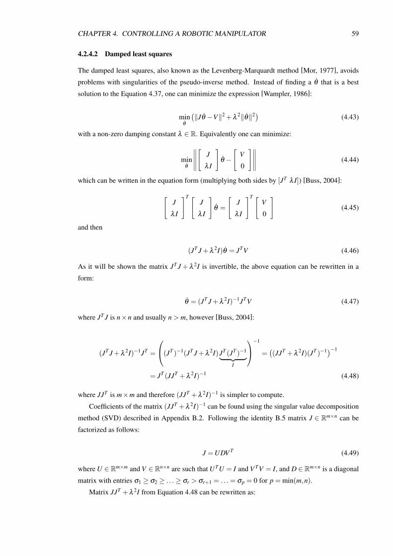
CHAPTER 4. CONTROLLING A ROBOTIC MANIPULATOR 59
4.2.4.2 Damped least squares
The damped least squares, also known as the Levenberg-Marquardt method [Mor, 1977], avoids
problems with singularities of the pseudo-inverse method. Instead of finding a θ that is a best
solution to the Equation 4.37, one can minimize the expression [Wampler, 1986]:
minθ
(‖Jθ −V‖2 +λ
2‖θ‖2) (4.43)
with a non-zero damping constant λ ∈ R. Equivalently one can minimize:
minθ
∥∥∥∥∥[
J
λ I
]θ −
[V
0
]∥∥∥∥∥ (4.44)
which can be written in the equation form (multiplying both sides by [JT λ I]) [Buss, 2004]:
[J
λ I
]T [J
λ I
]θ =
[J
λ I
]T [V
0
](4.45)
and then
(JT J +λ2I)θ = JTV (4.46)
As it will be shown the matrix JT J + λ 2I is invertible, the above equation can be rewritten in a
form:
θ = (JT J +λ2I)−1JTV (4.47)
where JT J is n×n and usually n > m, however [Buss, 2004]:
(JT J +λ2I)−1JT =
(JT )−1(JT J +λ2I)JT (JT )−1︸ ︷︷ ︸
I
−1
=((JJT +λ
2I)(JT )−1)−1
= JT (JJT +λ2I)−1 (4.48)
where JJT is m×m and therefore (JJT +λ 2I)−1 is simpler to compute.
Coefficients of the matrix (JJT +λ 2I)−1 can be found using the singular value decomposition
method (SVD) described in Appendix B.2. Following the identity B.5 matrix J ∈ Rm×n can be
factorized as follows:
J = UDV T (4.49)
where U ∈ Rm×m and V ∈ Rn×n are such that UTU = I and V TV = I, and D ∈ Rm×n is a diagonal
matrix with entries σ1 ≥ σ2 ≥ . . .≥ σr > σr+1 = . . . = σp = 0 for p = min(m,n).
Matrix JJT +λ 2I from Equation 4.48 can be rewritten as:

CHAPTER 4. CONTROLLING A ROBOTIC MANIPULATOR 60
JJT +λ2I = (UDV T )(V DTUT )+λ
2I = U(DDT +λ2I)UT (4.50)
The m×m matrix DDT +λ 2I is diagonal with entries σ2i +λ 2 > 0 for all i. Hence DDT +λ 2I is
non-singular and its inverse is a m×m matrix with entries (σ2i +λ 2)−1. The matrix given by 4.48
can now be written as:
JT (JJT +λ2I)−1 = (V DTUT )(U(DDT +λ
2I)UT )−1
= (V DTUT )(UT )−1(DDT +λ2I)−1U−1
= V DT (DDT +λ2I)−1UT = VAUT (4.51)
where A = DT (DDT +λ 2I)−1 ∈ Rn×m is a diagonal matrix with entries:
aii =σi
σ2i +λ 2 (4.52)
From Equation B.6 it follows that the matrix given by 4.51, i.e. a solution to the damped least
square method 4.47 can be written as:
JT (JJT +λ2I)−1 =
p
∑i=1
σi
σ2i +λ 2 viuT
i =r
∑i=1
σi
σ2i +λ 2 viuT
i (4.53)
where p = min(m,n), and where vi and ui are column vectors of matrices V and U .
It is clear that for λ > 0, the matrix 4.53 can be computed for any J. If λ = 0, the damped
least squares method reduces to the pseudo-inverse method as it is visible in Equation 4.43. If
σi → 0 for any i the matrix entries may become arbitrary large. If λ > 0 the matrix 4.53 also
behaves as pseudo-inverse J† if only σi� λ , however unlike J† all its entries are well-behaved in
the neighbourhood of singularities, i.e. when σi→ 0 for some i.
The damping constant λ decides the quality of solutions to Equation 4.47, however it should
not be chosen to be too small to avoid problems at singularities. Diagonal entries σi of D as well
as matrices U and V can be found as described in Appendix B.2.
4.2.4.3 Golem inverse instantaneous kinematics solver
The damped least squares method is also used in the Golem framework. It computes joint
velocities for a desired end-effector velocity using Jacobian 4.22 computed from the generic
formula for the spatial manipulator Jacobian 4.17.
4.3 Robot control
The position control of a robotic manipulator is a problem of finding motor commands such
that the manipulator body follows the desired trajectory. In a typical robotic manipulator motor
commands correspond to torques which are applied to joints through various actuators - e.g.

CHAPTER 4. CONTROLLING A ROBOTIC MANIPULATOR 61
electric motors. The dynamics of a robotic manipulator describes the dependency between the
motion of manipulator body parts and the applied actuator torques. Lagrangian formalism enables
expressing the manipulator dynamics in the form of a second-order differential equation which
relates actuator torques with joint variables and also directly with workspace coordinates of the
end-effector (see [Ortega and Spong, 1988] and [Murray et al., 1994]).
There are two common ways of controlling a robotic manipulator with respect to the desired
trajectory type4:
1. Joint space control specifies the control problem for a given desired trajectory in the
manipulator joint space.
2. Workspace control or operational space control specifies the control problem for a given
desired trajectory in the manipulator workspace, usually in terms of the position and
orientation of the end-effector.
Both types of the manipulator control are briefly presented in the following Sections 4.3.1 and
4.3.2. The last Section 4.3.3 describes the controller used in the Golem framework.
4.3.1 Joint space control
Joint space control addresses a problem of finding actuator torques τ ∈ Rn such that the robotic
manipulator follows the corresponding desired joint space trajectory θd(t) ∈ Rn, where n is the
number of manipulator joints. It is a problem of finding τ for a given instantaneous (at a particular
time t) desired joint position θd and velocity θd (also acceleration θd) using sensory feedback θ
and θ . A generic joint space controller is shown in Figure 4.6.
Controller Manipulator , d , d +
_
Figure 4.6: A generic joint space controller computes actuator torques τ such that the manipulator
follows a desired joint space trajectory θd(t), θd(t). The controller can also use sensory feedback
θ(t), θ(t) to correct the trajectory error.
The joint space control problem is not so simple because in general the dependency between
τ and θd is nonlinear for the following reasons:
1. The manipulator links are interconnected, a motion of a single joint which results from the
applied actuator torque depends on the configuration of the entire manipulator.4Other control methods can involve e.g. desired forces/torques applied to the manipulated objects

CHAPTER 4. CONTROLLING A ROBOTIC MANIPULATOR 62
2. A motion of a joint additionally depends on the current position and velocity of a joint due
to gravity, elasticity and friction.
3. Joint actuators are not linear devices, they also have limits on the maximum possible torques.
Lagrangian mechanics provides general methods to describe the motion of a mechanical
system which can account for the majority of the above dependencies. The motion of a
mechanical system is described by Lagrange equations which require specifying the kinetic and
potential energy of a modelled system [Arnold, 1989]. Solving Lagrange equations for a robotic
manipulator gives the following equations of motion (for derivation see [Murray et al., 1994] and
[Ortega and Spong, 1988]):
M(θ)θ +C(θ , θ)θ +N(θ , θ) = τ (4.54)
where θ(t) ∈Rn is the manipulator joint trajectory, τ ∈Rn are the actuator torques, M(θ) ∈Rn×n
is the manipulator inertia matrix, C(θ , θ)∈Rn×n is the Coriolis matrix and the term N(θ , θ)∈Rn
accounts for gravitation, friction and other external forces applied to joints.
The simplest control strategy can involve computing torque τ directly from the desired joint
trajectory {θd , θd , θd}:
M(θd)θd +C(θd , θd)θd +N(θd , θd) = τ (4.55)
The obtained open-loop control law is not however very robust, since does not take into account
the accumulating discrepancy between the actual state and the desired state. This discrepancy
is unavoidable in practice not only because it is difficult to create sufficiently good model of a
manipulator (in terms of M(θ), C(θ , θ) and N(θ , θ)), but also because of unmodeled external
forces applied during e.g. object manipulation.
Instead of controlling torques directly, one can require the manipulator to follow the trajectory
{θd , θd} and calculate the (nonlinear) torque needed to overcome the inertia of the manipulator
body by modifying the desired torque acceleration {θd}. It is the computed torque control law
which is defined as follows ([Ortega and Spong, 1988]):
M(θ)(θd−Kve−Kpe)+C(θ , θ)θ +N(θ , θ) = τ (4.56)
with trajectory error e = θ −θd , and where Kv and Kp are constant gain matrices. Equation 4.56
consists of two components which can be separated to give [Murray et al., 1994]:
M(θ)(θd)+C(θ , θ)θ +N(θ , θ)︸ ︷︷ ︸τ f f
+M(θ)(−Kve−Kpe)︸ ︷︷ ︸τ f d
= τ (4.57)
The feedforward component τ f f provides the amount of torque which would be sufficient to follow
a given trajectory if the manipulator was perfectly modelled by M(θ), C(θ , θ) and N(θ , θ). The

CHAPTER 4. CONTROLLING A ROBOTIC MANIPULATOR 63
feedback component τ f d provides the amount of torque which corrects any resultant trajectory
error.
The computed torque control law is an example of a feedback linearization method for
controlling a nonlinear system via nonlinear feedback which is represented by matrix components
(for details see e.g. [Spong, 1996]). The computed torque controllers are very robust, although
they are computationally expensive.
A PD controller is a simple alternative to the computed torque law, and can be seen as
linearised equation 4.56 (matrices M and C become diagonal):
τ =−Kve−Kpe (4.58)
where as before e = θ −θd , and Kv and Kp are constant gain matrices. The above formula has no
feedforward term providing additional torque which is necessary to follow exactly along a desired
trajectory. Frequently Equation 4.58 is extended by an additional integral term eliminating steady-
state errors (PID controller). Furthermore, if Kv and Kp are diagonal, Equation 4.58 can be split
into n independent equations, providing a simple way of controlling each joint separately.
4.3.2 Workspace control
Workspace control addresses the problem of controlling the robotic manipulator’s motion for a
given desired trajectory of the end-effector in the manipulator workspace coordinates gd(t) ∈SE(3), where gd(t) is assumed to be at least once differentiable (velocity control). The following
subsections briefly introduce two the most important ways of solving the workspace control
problem [Siciliano and Khatib, 2008].
4.3.2.1 Kinematics inversion
Controller Manipulator , d , d +
_Inversekinematics
g d , gd
Figure 4.7: A workspace controller realized as a combination of a joint space controller and an
inverse kinematics solver.
The simplest way of solving the workspace control problem is to find desired joint positions
θd and joint velocities θd which correspond to gd(t) and gd(t) and then use one of the joint
space controllers. This requires solving inverse kinematics and instantaneous inverse kinematics

CHAPTER 4. CONTROLLING A ROBOTIC MANIPULATOR 64
problems using for example algorithms described in Section 4.2. A workspace controller which
realizes these tasks is shown in Figure 4.7.
There are two major problems related to this kind of control approach:
1. Solving in real-time an inverse kinematics and instantaneous inverse kinematics can be a
CPU demanding task, even for modern computers.
2. Due to the nonlinearity of the forward kinematics map, trajectory errors which are decoupled
in the joint space will be no longer decoupled in the manipulator workspace. Consequently,
it is difficult to meaningfully control errors in the workspace by e.g. adjusting gain matrices
Kv and Kp of the computed torque controller in the joint space.
4.3.2.2 Direct workspace control
Controller Manipulator , +
_g d , gd Forward
kinematics
g , g
Figure 4.8: A generic workspace controller controls trajectory errors directly in the workspace.
It is possible to overcome some of the difficulties of using the joint space controller by
formulating the workspace control problem directly in the end-effector coordinates. A generic
workspace controller is shown on Figure 4.8.
So defined control problem requires parametrization of the forward kinematics mapping such
that gst : Rn→Rm where m is a number of parameters representing the rigid body transformation.
Differentiation of the mapping gst yields
x = Ja(θ)θ (4.59)
where Ja(θ) is the analytical Jacobian of gst (Section 4.2.2.2). Assuming that J has its inverse, the
following relationships hold:
θ = J−1x θ = J−1x+(
ddt
J−1)
x (4.60)
Substituting the above relationships into the Lagrange manipulator Equation 4.54 and multiplying
it by J−T = (J−1)T gives [Murray et al., 1994]:
J−T M(θ)J−1x+(
J−TC(θ , θ)J−1 + J−T M(θ)ddt
J−1)
x+ J−T N(θ , θ) = J−Tτ (4.61)

CHAPTER 4. CONTROLLING A ROBOTIC MANIPULATOR 65
which can be rewritten as [Murray et al., 1994]:
M(θ)J−1x+C(θ , θ)x+ N(θ , θ) = F (4.62)
where
M(θ) = J−T M(θ)J−1 (4.63a)
C(θ , θ) = J−TC(θ , θ)J−1 + J−T M(θ)ddt
J−1 (4.63b)
N(θ , θ) = J−T N(θ , θ) (4.63c)
F = J−Tτ (4.63d)
Equation 4.62 has the same structure as the manipulator Equation 4.54 defined in joint space
coordinates5. In particular the computed torque controller becomes:
M(θ)(xd−Kve−Kpe)+C(θ , θ)x+ N(θ , θ) = F (4.64)
where xd is the desired workspace trajectory, e = x− xd is the trajectory error, and Kv and Kp are
constant gain matrices.
4.3.3 Golem controller
A controller used in the Golem framework was designed to work mainly with the Katana
manipulator, therefore it also shares some of its limitations.
Katana 6M180 is an open-chain manipulator with five degrees of freedom (DOF) (plus one
degree for a gripper). The Katana provides an integrated PID controller with a separate control
of each joint actuator (diagonal gain matrices in Equation 4.58). However, the original Katana
firmware could accept only a small predefined number of joint trajectories represented by a set of
third degree polynomials in a form:
θd(t) = a3t3 +a2t2 +a1t +a0 (4.65)
where a0,a1,a2,a3 ∈ R are the polynomial coefficients and t = [0, tmax) is a time variable within a
given time interval. The trajectories had to be sent to the Katana PID controller prior to execution
of the movement. Therefore it was virtually impossible to create any more complex trajectory6.
This limitation has been removed thanks to cooperation with the Katana manufacturer
(Neuronics AG [Neuronics AG, 2004]). A new redesigned firmware is capable of accepting
single trajectories of the form of 4.65 online, one by one without interrupting the movement.
5It can be proven from Lyapunov stability theory that controllers built using the Equation 4.62 are stable as well[Murray et al., 1994]
6Consequently the original Katana user interface (Katana Native Interface) did not allow (and still does not) for a
true trajectory control.

CHAPTER 4. CONTROLLING A ROBOTIC MANIPULATOR 66
Furthermore, the firmware buffer has been redesigned to minimize communication latencies
between the controller and a PC interface.
4.3.3.1 Control modes
The Golem controller can operate in two modes:
1. In the joint space control mode the controller works according to the scheme 4.6. The
controller accepts sequences of pairs (θd , θd) which are subsequently transformed into third
degree trajectories 4.65 and sent to a manipulator. Each trajectory requires 4 parameters to
be fully specified, i.e. two consecutive pairs (θd , θd).
2. In the workspace control mode the controller works according to the scheme 4.7.
The controller accepts sequences of pairs (gd , gd) where gd is the desired end-effector
configuration. Configurations gd use angle-axis parametrization of rotation (Appendix
A). The corresponding pair (θd , θd) is computed using the inverse kinematics and inverse
instantaneous kinematics methods described in Subsection 4.2.4.3.
The inverse kinematics method 4.2.3.4 is based on the differential evolution optimization
algorithm (see Appendix C) with an initial population which is a set of joint variables {θ}.The population {θ}t at time t is generated only locally by sampling from a Gaussian with
a centre attached at the manipulator configuration θ t . The configuration θ t is obtained by
extrapolation of a trajectory polynomial from the previous time step t−1.
4.4 Robot planning
The motion planning for a robotic manipulator is the problem of finding a joint space trajectory
between a given initial configuration and a goal configuration of a manipulator. The initial and the
goal configurations can be specified in either the joint space or in the workspace of a manipulator.
By specifying some ad hoc trajectory between these configurations, motion planning can be also
considered as the joint space control problem or the workspace control problem respectively (see
Section 4.3). However in many cases a given fixed trajectory may not be feasible due to various
kinds of constraints imposed on the motion of a manipulator. Instead, one can search for a
trajectory such that it does not collide with obstacles while it can minimize various objectives
such as for example maximum velocity or acceleration of joints given the movement duration7.
Path planning is a basic instance of the motion planning problem that does not consider
differential constraints, i.e. constraints that are related to the velocity and the acceleration of
a manipulator body. The path planning problem for a robotic manipulator is introduced in
Section 4.4.1. Sampling-based approaches to the planning problem are among the most general
and successful ones and they are introduced in Section 4.4.2. Approaches which address the
7The motion planning problem can be further complicated by uncertainties, sensory feedback, etc. [LaValle, 2006].

CHAPTER 4. CONTROLLING A ROBOTIC MANIPULATOR 67
differential constraints are introduced in Section 4.4.3. The last section 4.4.4 describes the motion
planner used in the Golem framework.
4.4.1 Path planning problem
Two fundamental notions in the path planning problem involve:
1. The configuration space C or a C-space which is an Euclidean n-space - a set of all
possible configurations of a robot. A single element q ∈ C = Rn uniquely represents the
configuration a robot. The configuration space of a robotic manipulator corresponds to a set
of all possible joint variables θ (Section 4.1.2).
2. The workspace W which is an Euclidean m-space - a set of points Rm with m = 2 (plane)
or m = 3 (3D space). The workspace W should not be confused with the manipulator
workspace which is a space of positions and orientations of the end-effector of a manipulator
(Section 4.1.3).
The workspace W contains two closed subsets: an obstacle region O ⊂W and a robot body
A ⊂ W . O and A are usually represented as sets of geometric primitives. While an obstacle
region O is assumed to be static, a robot body A (q) is a function of its configuration q.
The C-space obstacle region Cobs is defined as:
Cobs = {q ∈ C : A (q)∩O 6= /0} (4.66)
The free space C f ree is a space of all configurations that avoids collisions:
C f ree = C \Cobs (4.67)
The path planning problem is defined as follows [Siciliano and Khatib, 2008]. For given:
1. Workspace W = Rm with m = 2 or m = 3
2. Obstacle region O ⊂W
3. Robot body A (q)⊂W which can be determined for any configuration q ∈ C
4. An initial configuration qI ∈ C f ree
5. A goal configuration qG ∈ C f ree
find a continuous path τ : [0,1]→ C f ree such that τ(0) = qI and τ(1) = qG.
A simplified version of the path planning problem known as the piano mover’s problem where
an obstacle region and a robot body are represented by polyhedra has been shown to be PSPACE-
complete [Reif, 1979]. However, if the differential constraints are taken into account, it is not
known yet if the problem is decidable except for some special cases [Cheng et al., 2007].

CHAPTER 4. CONTROLLING A ROBOTIC MANIPULATOR 68
4.4.2 Sampling-based approaches to path planning
Sampling-based planners make use of advances in modern collision detection algorithms which
are capable of efficiently computing whether a particular configuration q is collision free, i.e. if
q∈C f ree. A planner samples configuration space C and constructs a roadmap which approximates
collision free paths τ : [0,1]→C f ree. In this way a planner does not access the configuration space
directly, but only through a collision detection algorithm.
Sampling-based planners cannot assure that a collision-free path will be found in a finite time.
Despite this limitation sampling-based planners are capable of solving real-world problems which
are impractical to solve by complete approaches [Siciliano and Khatib, 2008].
A roadmap is represented as an undirected graph G(V,E) with a set of vertices V which are
sampled configurations in the free space C f ree and a set of edges E which are collision-free paths
determined by a local planner. Sampling-based planners are usually classified with respect to the
way in which the graph G(V,E) is constructed:
1. Multi-query planners construct a complete graph G(V,E) which approximates the connec-
tivity of the entire free space C f ree. Assuming that the obstacle region Oobs does not change,
multiple planning queries can be efficiently answered using the same initially created graph.
2. Single-query planners construct a graph G(V,E) online for each new planning query. To
efficiently answer a given query the single-query planners try to minimize the exploration
of the configuration space C .
Multi-query and Single-query planners are described in Section 4.4.2.1 and Section 4.4.2.2.
The most important sampling techniques are described in Section 4.4.2.3, local planners in Section
4.4.2.4, and finally collision detection techniques in Section 4.4.2.5. More details on sampling-
based planners can be found in a survey [Tsianos et al., 2007] and [Geraerts and Overmars, 2004].
4.4.2.1 Multi-query planners
Probabilistic Road Map (PRM) methods have been developed independently by different sites
[Overmars, 1992] [Kavraki and Latombe, 1994] [Kavraki et al., 1996] [Amato and Wu, 1996]
[Svestka, 1997]. PRM is an efficient and general approach which constructs a graph G(V,E)
approximating the connectivity of the entire free space C f ree. A typical PRM method constructs
G(V,E) using the following procedure (also see [Siciliano and Khatib, 2008]):
1. Initialize G(V,E) with an empty set of vertices V and an empty set of edges E.
2. Sample a random configuration s ∈ C f ree using sampling techniques from Section 4.4.2.3.
3. Find all neighbouring vertices q from G(V,E) such that their distance µ to s is small enough
given some predefined metric d, e.g. d : C ×C → R.

CHAPTER 4. CONTROLLING A ROBOTIC MANIPULATOR 69
s
Cobs
Cobs
C free
Figure 4.9: In each iteration of the PRM method, for a sampled configuration s, the neighbouring
vertices q within a predefined distance µ are selected. Then, for each neighbouring vertex q the
method tries to construct a collision-free path to s (dashed lines). Each collision-free local path is
inserted to the graph as an edge (continuous lines).
4. For each neighbouring vertex q attempt to construct a collision-free path τlocal : [0,1]→C f ree such that τlocal(0) = s and τlocal(1) = q using one of the local planners from Section
4.4.2.4.
5. If the path τlocal is found insert it into G(V,E) as an edge.
6. Break the procedure if a termination condition is satisfied - e.g. a total number of vertices
of G(V,E) equals to some predefined limit. Otherwise return to step 2.
A single iteration of the PRM method is shown on Figure 4.9. Vertices in the graph G(V,E)
comprise clusters which may (a single cluster) or may not (multiple clusters) be interconnected by
edges (local paths).
In order to solve a planning query an initial and a goal configuration qI,qG ∈ C f ree are added
to the graph. If the query configurations belong to the same graph cluster, a shortest (optimal) path
can be found using e.g. A? algorithm (Section D). If the query configurations do not belong to the
same graph cluster, a continuous path connecting qI and qG does not exist. New vertices can be
added to the graph or the entire graph can be rebuilt.

CHAPTER 4. CONTROLLING A ROBOTIC MANIPULATOR 70
4.4.2.2 Single-query planners
Single-query planners focus on efficient answering a single planner query. They explore the
configuration space by generating incrementally tree data structures initialized at known (usually
at initial and goal) configurations eventually connecting them. A typical single-query planner
constructs a graph G(V,E) using the following tree-expansion procedure [Siciliano and Khatib,
2008]:
1. Initialize G(V,E) with an empty set of edges E and a set of vertices V which includes at
least an initial configuration qI ∈ C f ree.
2. Select a local initial configuration s ∈ V , and a local goal configuration u which may or
may not be in V . If there can be no other goal configurations u selected, or some other
termination condition is satisfied, report a failure and break the procedure.
3. Attempt to construct a collision-free path τlocal : [0,1]→ C f ree such that τlocal(0) = s and
τlocal(1) = u using one of the local planners from Section 4.4.2.4.
4. If the path τlocal is found insert it into G(V,E) as an edge and insert u as a vertex if it is not
already in V . Otherwise return to step 2.
5. If the graph G(V,E) contains a solution path from qI to qG, report a success and break the
loop. Otherwise return to step 2.
Path search performed by the above procedure generates a tree rooted at the configuration s
from the first iteration. Unidirectional planners generate a tree rooted at a single configuration,
usually qI . Bidirectional (see for example [Kuffner Jr and LaValle, 2000]) and multidirectional
(see for example [Plaku et al., 2005]) planners use two and more such configurations - qI , qG or
configurations placed e.g. near narrow passages to avoid being trapped. One of the drawbacks
of using more than a one tree is an increasing difficulty of determining the optimal connections
between them.
The tree-expansion procedure critically depends on the second step where the (local) initial
and goal configurations are selected for further tree expansion.
Rapidly exploring random trees (RRT) [LaValle, 2001] bias tree-expansion towards a Voronoi
region proportionally to its volume. A generalized version of RRT, rapidly exploring dense trees
(RDT) use a bidirectional search generating two trees rooted at qI and qG [LaValle, 2006]. RDT
spends roughly half of the time expanding the trees and the other half trying to connect them.
Heuristically-guided random trees [Urmson and Simmons, 2003] bias the search towards low-
cost paths using a total cost of the path from the initial configuration qI and estimation of the
remaining cost to a goal configuration qG. Similar principles are exploited in [Diankov and
Kuffner, 2007] using a version of the A? graph search algorithm. Utility-guided random trees
[Burns and Brock, 2007] evaluate several aspects of the tree expansion: the utility value of the
configuration s to be expanded, the expansion distance and direction and connection attempts.

CHAPTER 4. CONTROLLING A ROBOTIC MANIPULATOR 71
4.4.2.3 Sampling techniques
The efficiency of sampling-based planners largely depends on a way in which vertices V of the
graph G(V,E) are generated. Vertices are samples of the free configuration space s ∈ C f ree. The
most popular sampling techniques of the entire configuration space C are listed below [Geraerts
and Overmars, 2004] [LaValle, 2006]:
• Random methods generate samples with uniformly generated random coordinates in the
allowable configuration space C . The corresponding poses of a robot in a workspace may
not be uniformly spread due to the nonlinearity of the forward kinematics map.
• Grid methods choose samples on a grid. The process starts with some initial grid resolution,
subsequently doubling it every step until the required grid resolution is obtained.
• Cell-based methods attempt to generate uniformly spread samples in the workspace. The
procedure generates samples within a single cell in the workspace, divides it into 2D sub-
cells for D = 2 or D = 3 and repeats the process within each sub-cell.
The C-space obstacle region Cobs can occupied critical regions of the configuration space. There
have been developed several techniques which either generate samples between obstacles or close
to obstacle boundaries, for example [LaValle, 2006]:
• Voronoi region-based methods [Wilmarth et al., 1999][LaValle, 2001] generate samples
near Voronoi regions of obstacles.
• A Gaussian sampling method generates samples near obstacles using Gaussian distribution
and two samples such that one lies in the free space C f ree while the other in the obstacle
region Cobs [Boor et al., 1999].
4.4.2.4 Local planners
Local planners attempt to construct a collision free path connecting the local initial and the local
goal configurations s,u ∈V of the graph G(V,E). There is a trade-off between the ability to create
collision free paths and the efficiency of a planner expressed in terms of the number of attempted
connections per unit of time. Furthermore, local planners should be deterministic to avoid storing
parameters of each local path connecting graph nodes.
Although there exist other methods [Amato et al., 1998], in majority of cases the optimal
strategy is to choose a simple straight line local path in the configuration space. The path can then
be efficiently tested for collisions as described in Section 4.4.2.5.
4.4.2.5 Collision detection
A path generated by a local planner needs to be determined if it is collision free, i.e. if
τlocal : [0,1]→ C f ree for a given τlocal(0) = s and τlocal(1) = u. Testing for collisions a continuum

CHAPTER 4. CONTROLLING A ROBOTIC MANIPULATOR 72
of configurations on the path τlocal can be very expensive therefore the majority of methods use
only a discrete set of configurations lying on the path. Collision detection algorithms can then
be abstracted as a simple black-box boolean-valued function f f ree : C → {true, f alse} which
indicates if a particular configuration q ∈ C is collision free (true) or not ( f alse) 8.
There are two most important methods of discretization of the local path used [Geraerts and
Overmars, 2004]:
1. An incremental method performs a collision check in small steps starting from configuration
s to u or from u to s.
2. A binary method checks a middle configuration on the path and if the configuration is
collision free, the method recursively checks the two created halves of a path in a breath-first
manner.
The collision detection function f f ree : C → {true, f alse} checks if a robot body A (q) ⊂W represented as a set of n geometric primitives (robot links) A1(q), . . . ,An(q) for a given
configuration q, collides with an obstacle region O ⊂ W represented as a set of m geometric
primitives O1, . . . ,Om. The function f f ree has to test for collisions each pair of geometric primitives
from a set A1(q), . . . ,An(q),O1, . . . ,Om.
There is a performance trade-off between the number of primitives and the representational
complexity of a single geometric primitive. Collision checking between planes, spheres, capsules
or cylinders is significantly faster than between non-convex polyhedra. On the other hand
representations of bodies as sets of such simple geometric primitives may not be sufficient. One
way to alleviate this problem is to decompose each body into a tree [LaValle, 2006]. Vertices of
a tree represent bounding primitives that contain some subsets of primitives comprising the body.
A bounding primitive which corresponds to the root contains all body geometric primitives. The
method avoids unnecessary collision checks between bodies’ primitives if the two tested bodies are
far apart. It recursively tests for collisions in the bounding primitives hierarchy only if a collision
is detected at a higher level of the hierarchy.
4.4.3 Incorporating differential constraints
Differential constraints limit the velocity q and also the acceleration q of the moving robot’s body.
Because they depend on the current configuration q ∈ C they are referred as to local constraints,
in contrast to global constraints represented by obstacle region O ⊂W .
Differential constraints on C are usually expressed in the form of a state transition equation
x = f (x,u) where u ∈ U is an action chosen from action space U , and x ∈ X represents both a
configuration and velocity x = (q, q) from a state space X of C-space.
By ignoring velocity q, one can define the obstacle region Xobs as:
8In order to improve collision detection performance some algorithms can also return information about a distance
between obstacles’ boundaries [Jimenez et al., 2001]

CHAPTER 4. CONTROLLING A ROBOTIC MANIPULATOR 73
Xobs = {x = (q, q) ∈ X : A (q)∩O 6= /0} (4.68)
The region of inevitable collision Xric takes into account velocity q [LaValle, 2006]:
Xric = {x(0) ∈ X : for any u ∈U∞,∃t > 0 such that x(t) ∈ Xobs} (4.69)
where x(t) is a state at time t obtained by integrating the action trajectory which is a function of
the form u : [0,∞)→U from a set of all possible action trajectory functions U∞:
x(t) = x(0)+∫ t
0f (x(t ′),u(t ′))dt ′ (4.70)
The existence of Xric which always subsumes Xobs shows that planning methods introduced in
the previous section may need to be extended to fully address differential constraints. Traditionally
three categories of the planning problem under differential constraints are considered [LaValle,
2006]:
1. Nonholonomic planning incorporates nonholonomic constraints which cannot be converted
into constraints that do not involve derivatives. The term was originally introduced for
wheeled mobile robots which cannot move sideways.
2. Kinodynamic planning incorporates constraints on at least velocity and acceleration on C
in a form of an equation x = f (x,u). Nonholonomic planning can also be seen as a form of
kinodynamic planning.
3. Trajectory planning is a problem of determining the path and velocity of a moving robot
body. The problem can be considered as a version of kinodynamic planning that includes
only velocity constraints.
The following subsections present briefly some of the most important group of approaches
developed to address a problem of planning under differential constraints [LaValle, 2006]. The last
subsection 4.4.3.2 describes decoupled approaches which includes a method used by the Golem
planner.
4.4.3.1 Kinodynamic planning
The kinodynamic planning problem can be addressed directly in the state space X using sampling.
Sampling-based approaches explore the state space X by constructing one or more reachability
trees, usually on a lattice. This requires discretization of action space and time. Reachability trees
do not need to form a regular lattice. RRT [LaValle, 2001] can be used directly in the state space.
RRT expands trees in a random fashion covering new space in an efficient way.
Although methods from this group provide a probabilistic completeness guarantee [LaValle,
2006], they are computationally expensive mainly due to the high dimensionality of X .

CHAPTER 4. CONTROLLING A ROBOTIC MANIPULATOR 74
4.4.3.2 Decoupled approaches
Approaches from this group split a planning problem with differential constraints into a set of
simpler problems. A typical decoupled approach procedure is shown below [LaValle, 2006]:
Path planing. Find a collision-free path τ : [0,1]→ C f ree ignoring differential constraints. Use
one of the introduced path planning algorithms from Section 4.4.1.
Path optimization. Transform path τ into a new path τ ′ so that velocity constraints on C are
satisfied. This step usually involves path smoothing.
Path profiling. Compute a timing function σ : [0,T ] → [0,1] for τ ′ so that σ ◦ τ ′ is a time
parametrized path on C f ree. The state space trajectory x(t) must satisfy x = f (x(t),u(t))
in the time interval [0,T ].
Trajectory control. Choose a feedback control law π : X→U which minimizes the error between
a desired and measured state.
Methods presented in Section 4.4.3.1 are capable of solving steps 1-2 or even 1-3 for low
dimensional problems. Methods from Section 4.3 address the control problem in the step 4.
4.4.4 Golem trajectory planner
The Golem trajectory planner follows a typical procedure from the decoupled approach group
from Section 4.4.3.2. The procedure steps are described in more details in the following sections.
4.4.4.1 Path planning
The Golem path planner is a single-query planner realized as a heuristically-guided random tree
which expands using the A? graph search algorithm (see Figure 4.10).
Vertices of a graph G(V,E) are a combination of uniform sampling of the joint coordinates
(as in random methods from Section 4.4.2.3) and vertices generated from Gaussians localized at
joint configurations called generators. There are at least two generators specified - an initial and
a goal configurations θI,θG ∈ C f ree. Similarly as in Gaussian sampling methods (Section 4.4.2.3)
generators can facilitate path searching in narrow passages between objects.
Heuristic function f used by the A? graph search algorithm (see Appendix D) estimates the
cost of moving from configuration θi ∈ C f ree to θ j ∈ C f ree for a given goal θG ∈ C f ree and “home”
configuration θhome ∈C . Home configuration θhome limits the variability of joints (the manipulator
internal motion) which are in the manipulator Jacobian null space similarly as in the Golem inverse
kinematics solver (Section 4.2.3.4). Heuristic function f is a linear combination of the following
functions:
f = wdist fdist(θi,θ j)+wgoal fgoal(θ j,θG)+whome fhome(θ j,θhome) (4.71)

CHAPTER 4. CONTROLLING A ROBOTIC MANIPULATOR 75
Figure 4.10: The Golem path planner generates a number of collision-free manipulator
configurations (yellow dots) and then runs the A? graph search algorithm to find a path (cyan line
segments) in the obstacle field (transparent grey boxes) between an initial and goal configurations.
where wdist ,wgoal,whome ∈ R are normalizing weights. Functions fdist , fgoal , fhome provide a
bounded distance between two specified joint configurations θi and θ j and are defined as below:
fgoal,home(θi,θ j) = ‖θ j−θi‖2 (4.72)
fdist(θi,θ j) = w joint‖θ j−θi‖2 +wpos fpos(θi,θ j)+wrot frot(θi,θ j) (4.73)
where ‖ ∗ ‖ is the Euclidean distance (norm). fpos(θi,θ j) and frot(θi,θ j) measures linear and
angular distance between the end-effector workspace configurations corresponding to the joint
configurations θi and θ j. fpos and frot are defined as in Equation 4.32 and Equation 4.33.
Local planner uses a typical straight line search. An incremental or (as an option) binary
collision detection method is used (Section 4.4.2.5). Geometric primitives involve only convex
shapes: planes, spheres, cylinders, boxes and convex meshes.
4.4.4.2 Local path planning
Initial path τ generated by the path planner shown in Figure 4.10 has to be further optimized.
However because path optimization additionally takes into account differential constraints, the
entire optimization process is usually time consuming and solutions can be easily trapped in local
minima.
One of the methods of avoiding some of these problems is to re-run the above path planning
procedure “locally”. The local path planning generates (using generators) a new set of “local”

CHAPTER 4. CONTROLLING A ROBOTIC MANIPULATOR 76
Figure 4.11: The Golem path planner re-runs the basic path planning procedure by generating
a new set of “local” vertices (yellow dots) in the neighbourhood of the initial path (cyan line
segments) and find a new local path (magenta line segments).
vertices of a graph Glocal(V,E) in the neighbourhood of initial path τ and find a new local path
τlocal connecting the same initial and goal configurations θI,θG. The Golem path planner re-runs
the local path planning procedure a small predefined number of times simultaneously decreasing
a distance threshold dmax in function isExpandable() in the A? graph search algorithm (see
Appendix D). The resultant path is shown in Figure 4.11.
4.4.4.3 Path optimization
A local path consists of N joint configurations τlocal = {θ1, . . . ,θN} ∈ C f ree such that θ1 = θI and
θN = θG. There is also given a velocity profile:
v(s) : [0,1]→ R (4.74)
where s ∈ [0,1] is a normalized path distance computed along a given path τ using function fdist
given by Equation 4.73.
τlocal is optimized with respect to the acceleration and velocity constraints using a procedure
similar to the simulated annealing (see Appendix C):
1. Pick randomly a configuration θi ∈ τlocal such that i = 2 . . .N−1.
2. Generate a new configuration θ ∗i using the following procedure:
θ∗i, j = θi, j + ri, jrand(−∆T,+∆T ) (4.75)

CHAPTER 4. CONTROLLING A ROBOTIC MANIPULATOR 77
Figure 4.12: The Golem path optimization procedure computes an optimized path (black line
segments with local coordinate frames) with respect to the acceleration and velocity constraints.
where j is a coordinate index, rand() randomly generate a value within the specified range,
∆T is selected according to the logarithmic annealing schedule (Appendix C) and ri, j is an
estimate of variability of θi, j approximated as below:
ri, j = c0j +
i+l
∑k=i−l
ckj|θk−1, j−θk+1, j| (4.76)
where l > 0 and ckj > 0 are predefined constants.
3. Find the energy difference ∆E between the new state θ ∗i and the previous state θi:
∆E = E(θ ∗i )−E(θi) (4.77)
The state energies E(θ ∗i ) and E(θi) are computed as follows:
E(θi) = fdist(θi,θi−1)+ fdist(θi,θi+1)+wvelfdist(θi+1,θi−1)
∆ti(4.78)
where fdist is given by Equation 4.73 and where the last term represents a velocity penalty
for a given constant wvel and a time delta ∆ti estimated for a specified θi and a velocity
profile given by Equation 4.74.
4. Accept a new configuration θ ∗i if ∆E < 0 or a random number p ∈ [0,1] is smaller than
exp(−∆E/kBT ). However, do not accept the configuration θ ∗i if the new path segments
CHAPTER 4. CONTROLLING A ROBOTIC MANIPULATOR 78
cause a collision or if fdist(θ ∗i ,θi−1) or fdist(θ ∗i ,θi+1) are higher than some predefined
minimum distance.
5. Break the procedure after a predefined number of steps has been completed (proportional to
the entire length),
An example optimized path τopt after approx. 2000 iterations is shown in Figure 4.12.
4.4.4.4 Path profiling
The Golem path profiling procedure for each configuration θi ∈ τopt finds corresponding velocity
θi by differentiation a 3-rd degree polynomial which can be determined from the (path) neighbours
of θi. The resultant pairs θi and θi comprise a complete joint space trajectory.
4.4.4.5 Trajectory control
A joint space control method which transforms a sequence of pairs θi and θi into corresponding
torques is described in Section 4.3.3.1.
4.5 Summary
This chapter introduced methods which are implemented in the Golem software framework and
used in all robotic experiments in this thesis. A typical pushing experiment as described e.g. in
Section 3.1 consists of at least two parts:
1. An approach movement to the initial pose of a forward pushing movement.
2. A forward movement towards an object.
During a single experiment both parts are usually repeated several times. The approach
movement uses methods of path planning with collision detection described in Section 4.4.4.3.
Collision detection is particularly important at the beginning and at the end of the experiment
where a manipulator has to safely move from and to its home position among various obstacles
(usually a table but not only).
The forward movements are realized using a workspace control method described in
Section 4.3.3. The workspace straight line trajectory is generated online from a velocity profile
(Equation 4.74) and the starting and the final poses of the end-effector (via interpolation).
Although, the presented algorithms are mostly based on the state-of-art algorithms for the
manipulator control and path planning, there are a few minor contributions. Most importantly a
local path planning method (Section 4.4.4.2) and an optimization method for the final trajectory
of a robotic manipulator (Section 4.4.4.3).

Chapter 5
Prediction learning in robotic pushingmanipulation
This chapter addresses the problem of learning to predict how objects behave under simple robotic
pushing actions, i.e. a problem of learning of forward models in pushing manipulation. As
described in Chapter 2 and Chapter 3, forward models play a central role in many sensorimotor
control frameworks. Furthermore, Chapter 3 argues that the learning of forward models for
manipulated objects could offer several benefits over using for example physics simulators.
Unfortunately, because of the variability of the shape and other properties of the physical objects,
learning of such models poses some additional difficulties, as opposed to learning of forward
models for a robot body alone1.
This chapter formulates the prediction problem for a manipulated object as a problem of
predicting a rigid body transformation of the object given the movement of a robotic manipulator.
Such simple but generic forward models can be learned purely from experience providing that
the given object and environment are fixed. This approach might not be very practical however,
especially in situations where the object shape and other physical properties are changing. The
subsequent sections propose various improvements which make use of additional knowledge, e.g.
about the object contacts or the centre of mass. In particular, a method using the product of contact
experts is proposed to allow better generalization over the object shape and applied actions. All the
introduced models are experimentally tested in a virtual environment as well as in real experiments
using 5-axis Katana robotic manipulator with a vision-based tracking system.
The chapter consists of the following sections:
• Section 5.1 introduces basic representations used in forward models in this chapter. The
section discusses various problems related to learning of these models, in particular
the dimensionality problem and the problem of generalization across many objects with
different physical properties. The section also proposes a simplifying quasi-static world
assumption which is used throughout the rest of the chapter.1The configuration and properties of the body of a robot are usually assumed constant.
79

CHAPTER 5. PREDICTION LEARNING IN ROBOTIC PUSHING MANIPULATION 80
• Section 5.2 formulates the prediction learning problem as a problem of function estimation
(regression) using representations introduced in the previous section. The section briefly
discusses some of the shortcomings of this approach.
• Section 5.3 formulates the prediction learning problem as a density estimation problem. The
most likely prediction can be found as a maximum of a product of probability densities,
where each density is an expert specialized in predicting the behaviour of a particular
contact between interacting objects’ shape parts. The chapter also describes a kernel density
estimation method used to implement the forward model.
• Section 5.4 proposes evaluation criteria for the introduced forward models. The section
describes experiments which have been used to test the models in a virtual environment as
well as in real experiments using a system composed of the Katana robotic manipulator with
a vision-based tracking system.
• Section 5.5 summarizes the chapter and briefly discusses future work on forward models in
pushing manipulation.
5.1 Representing interactions of rigid bodies
5.1.1 A three body system
At
Finger Object
Environment
TAt , Bt
TBt ,O
Bt
O
Figure 5.1: 2D projection at time t of a robotic finger with frame At , an object with frame Bt , and
a ground plane with constant frame O.
Consider three reference frames A, B and O in a 3-dimensional Cartesian space. For example
frame A can represent a robotic finger which pushes an object with frame B which in turn is placed
on a table top with frame O as in Figure 5.1. While frame O is fixed, A and B change in time and
are observed at discrete time steps ..., t−1, t, t +1, ... every non-zero ∆t. A frame X at time step t
is denoted by Xt , a rigid body transformation between a frame X and a frame Y is denoted by T X ,Y
(see Figure 5.2).
From classical mechanics we know that in order to predict a state of a body, it is sufficient to
know its mass, velocity and a net force applied to the body. We do not assume any knowledge of

CHAPTER 5. PREDICTION LEARNING IN ROBOTIC PUSHING MANIPULATION 81
Figure 5.2: A system consisting of three interacting bodies with frames A and B in some constant
environment with frame O can be described by six rigid body transformations T At ,Bt , T Bt ,O,
T At−1,At , T At ,At+1 , T Bt−1,Bt , and T Bt ,Bt+1 .
the mass and applied forces, however the transformations of a body, with attached frame B, over
two time steps T Bt−1,Bt and T Bt ,Bt+1 encode its acceleration - the effect of the applied net force.
Therefore, if the net force and the body mass are constant, the transformations T Bt−1,Bt and T Bt ,Bt+1
provide a complete description of the state of a body at time step t in absence of other bodies. A
triple of transformations T Bt ,O, T Bt−1,Bt and T Bt ,Bt+1 provide a complete description of a state of a
body in some fixed frame of reference O which accounts for a constant or stationary environment.
Similarly, transformations T At ,O, T At−1,At and T At ,At+1 provide such a description for some other
body with frame A.
The state of a system consisting of three bodies with frames A and B in some constant
environment with frame O can be described by the six transformations as it is shown in Figure 5.2,
where T At ,O has been replaced by a relative transformation T At ,Bt . The transformation T Bt ,O can
be omitted, if the environment does not affect the motion of the bodies or it is explicitly modelled
by one of them.
5.1.2 Body frame representation
We expect that the behaviour of interacting bodies represented by rigid body transformations as
in Figure 5.2 shares some statistical similarities independently on their global poses with respect
to some current inertial frame I. Consider two scenes (1) and (2) as shown in Figure 5.3. A
pose change between time step t and t + 1 as observed in instantaneous object body frame A(1)
and the same object in another instantaneous body frame A(2) given inertial frame I are both
the same. However because transformations T I,A(1)and T I,A(2)
are different, the corresponding
transformations in the inertial frame (with subscript i) are also different, i.e. TA(1)
t ,A(1)t+1
in 6= TA(2)
t ,A(2)t+1
in .
Instead of using inertial frame-dependent transformation T At ,At+1in , one can represent object
transformations as observed in the object body frame. Body frame transformation T At ,At+1body (with

CHAPTER 5. PREDICTION LEARNING IN ROBOTIC PUSHING MANIPULATION 82
At1
TI , At
1
I
TI , At1
1
At11
T inAt1 , At1
1
At2
TI , At
2
I
TI , At1
2
At12
T inAt2 , At1
2
Figure 5.3: In the above two scenes a pose change between time step t and t + 1 as observed in
instantaneous object body frame A(1) and the same object in another instantaneous body frame
A(2) given inertial frame I are both the same. However because transformations T I,A(1)and
T I,A(2)are different, the corresponding transformations in the inertial frame are also different, i.e.
TA(1)
t ,A(1)t+1
in 6= TA(2)
t ,A(2)t+1
in .
At1T bodyAt , At1
I=At
Figure 5.4: The body frame transformation T At ,At+1body represents movement instantaneous object
frame At at time t overlaps with inertial frame I.
subscript b) is obtained by moving instantaneous frame A, so that at time t it overlaps with inertial
frame I (see Figure 5.4). Given some instantaneous object frame At at time t, transformation
T At ,At+1in and because T I,At+1 = T At ,At+1
in T I,At = T I,At T At ,At+1body , one can obtain transformation T At ,At+1
body
in the body frame as follows (also see Appendix A):
T At ,At+1body = (T I,At )−1T At ,At+1
in T I,At (5.1)
Similarly from a given transformation in body frame, instantaneous object frame At at t and using
Equation 5.1, one can obtain expression for transformation T At ,At+1in in the inertial frame
T At ,At+1in = T I,At T At ,At+1
body (T I,At )−1 (5.2)
If not stated otherwise in further discussion we will keep subscripts in while dropping
subscripts body assuming that all transformations T X ,Y are transformations in the body frame
X obtained from T X ,Y ≡ T X ,Ybody = (T I,X)−1T X ,Y
in T I,X .

CHAPTER 5. PREDICTION LEARNING IN ROBOTIC PUSHING MANIPULATION 83
5.2 Prediction learning as a regression problem
The prediction problem can now be stated as: given we know or observe the starting states and
the motion of the pusher, T At ,At+1 , predict the resulting motion of the object, T Bt ,Bt+1 . This is a
problem of finding a function:
f : T At ,Bt ,T Bt ,O,T At−1,At ,T Bt−1,Bt ,T At ,At+1 → T Bt ,Bt+1 (5.3)
Function 5.3 is capable of encoding all possible effects of interactions between rigid bodies A
and B, providing their physical properties and applied net forces are constant in time. Furthermore,
it can be learned purely from observations for some fixed time delta ∆t.
There are two problems related to relying on such a function:
1. Limited or no generalization capability. A function approximating interactions between
bodies A and B cannot be used for any other bodies of e.g. different shape or mass. This is
because function 5.3 implicitly encodes information about the surfaces of A and B, which
play a critical role in collisions. In this way a slight change of the objects’ shape can
cause a dramatic deviation of the predicted transformation T Bt ,Bt+1 . Consequences of surface
deformations are further discussed in the experimental section 5.4.
2. Dimensionality problem. For a rigid body transformation represented as a set of 6 or
7 numbers, the domain of function 5.3 has 30 or 35 dimensions. This problem can be
alleviated by a quasi-static assumption introduced in the following section 5.2.1.
5.2.1 Quasi-static assumption
Frame A Frame B
At1
TAt , Bt T
Bt , Bt1TAt , At1 At
Bt1
Bt
TBt ,O
O
Figure 5.5: In quasi-static conditions two interacting bodies with frames A and B in constant
environment with frame O can be described by only four rigid body transformations T At ,Bt , T Bt ,O,
T At ,At+1 and T Bt ,Bt+1 .
CHAPTER 5. PREDICTION LEARNING IN ROBOTIC PUSHING MANIPULATION 84
In many robotic operations, manipulations are slow, one can assume quasi-static conditions,
and it is often possible to ignore all frames at time t − 1 as it is shown in Figure 5.5.
This conveniently reduces the dimensionality of the problem to 18 dimensions if rigid body
transformations are represented by 6 numbers using e.g. Euler angles. Function 5.3 can then
be rewritten in a simpler form:
f : T At ,Bt ,T Bt ,O,T At ,At+1 → T Bt ,Bt+1 (5.4)
The quasi-static assumption comes at a price however. Function 5.4 no longer encodes the
complete information about a state of the system, in particular the velocity of frame A and B.
For example transformations T At ,Bt ,T Bt ,O,T At ,At+1 comprising the domain of Function 5.4 can be
exactly the same for two very different situations. In the first situation a robotic finger approaches
a non-moving (yet) object, while in the second the object begins to move after being pushed by
the finger. Still the movement of the finger, the relative pose between the finger and the object as
well as the object pose on the table are all the same. This ambiguity can be removed by encoding
explicitly the causal relation between the finger movement and the object movement. In order to
do this, two phases of the approaching before touching the object and after touching are split by
detecting a moment the finger touches the object2.
5.3 Predicting rigid body motions using multiple experts
5.3.1 Combining local and global information with two experts
It is clear that we need to enable generalization of predictions with respect to changes in shape.
Consider two objects lying on a table top. Figure 5.6 shows two situations that are identical except
for the shape of object A. It is clear that the same transformation of A’s position will lead to
different motions for object B in each case, mostly due to a potentially infinite number of ways
shapes A and B can vary. How can we then encode the way in which the shapes of A and B alter
the way they behave? We use a product of several densities to approximate the density over the
rigid body transformation instead of a single value as given in the function 5.4.
In the simplest case one can approximate two densities, conditioned on local and global
information respectively. We define the global information to be the information about changes
of the pose of the whole object. The local information is specified by changes of the pose of the
surfaces of A and B at the contact point, or the point of closest proximity, between the object and
the finger. We model this local shape as a pair of planar surface patches, of limited extent (see
Figure 5.7). Statistically, the greater the starting distance between these local surface patches of A
and B, and/or the smaller the magnitude of the transformation T At ,At+1 , the less likely it is that the
objects will collide, and hence the less likely it is that the pose of shape B will change between
t and t + 1, or equivalently the more likely that the transformation T Bt ,Bt+1 will be an identity
2In practice no algorithm could work without applying this trick.

CHAPTER 5. PREDICTION LEARNING IN ROBOTIC PUSHING MANIPULATION 85
At
At1
Bt=B t1
At1At
Bt
Bt1
Figure 5.6: Two scenes, each with two objects on a table top, viewed from above. Between the
two scenes only the shape of A is different. Yet when A moves the resulting transformation T Bt ,Bt+1
will be quite different. This shows that our predictors must take some aspect of the shape of A and
B into account.
transformation Id. On the other hand, if the local surfaces A and B are close a large portion of
possible transformations T At ,At+1 will cause collisions.
AtTAt , B t
BtTBt , Bt1
TAt , At1
At1
Bt1
AtTAt , B t
BtTBt , Bt1
TAt , At1
At1
Bt1
Figure 5.7: Two scenes, each with two objects on a table top, viewed from above. Local shapes
A and B, transformations T At ,At+1 and T At ,Bt are the same in each scene. Still, the transformation
T Bt ,Bt+1 is different because local shapes belong to different parts of objects.
Transformations T At ,Bt , T At ,At+1 and T Bt ,Bt+1 , observed over many experimental trials for many
different objects form a conditional distribution:
{T Bt ,Bt+1 |T At ,At+1 ,T At ,Bt} (5.5)
While conditional distribution 5.5 for global frames may become unimodal, for local shapes is
highly multi-modal. To see this consider two scenes with two objects, where the initial conditions
are identical (Figure 5.7). Local shapes A and B, transformations T At ,At+1 and T At ,Bt are the same
in each scene. Still, the transformation T Bt ,Bt+1 is different because local shapes belong to different
parts of objects.

CHAPTER 5. PREDICTION LEARNING IN ROBOTIC PUSHING MANIPULATION 86
At
Finger Object
EnvironmentTAtl , Bt
lBtl
TAt , Bt
TBt ,O
Atl
Bt
O
Figure 5.8: 2D projection at time t of a robotic finger with global frame At , an object with global
frame Bt , and a ground plane with constant global frame O. Local frames Alt and Bl
t describe the
local shape of the finger and an object at their point of closest proximity.
Consider a 2D projection at time t of a robotic finger with global frame At , an object with
global frame Bt , and a ground plane with constant global frame O (Figure 5.8). Similarly, local
frames Alt and Bl
t describe local shapes belonging to a finger and an object. The global conditional
density function can be defined as:
pglobal(T Bt ,Bt+1 |T At ,At+1 ,T At ,Bt ,T Bt ,O) (5.6)
and similarly a local conditional density function as:
plocal(T Blt ,B
lt+1 |T Al
t ,Alt+1 ,T Al
t ,Blt ) (5.7)
The only problem is to determine the above three transformations in the body frame of the local
shapes. For a particular situation shown in Figure 5.8 from object rigidity and using Equation 5.1
we have:
T Alt ,A
lt+1 = (T I,Al
t )−1T At ,At+1in T I,Al
t (5.8a)
T Blt ,B
lt+1 = (T I,Bl
t )−1T Bt ,Bt+1in T I,Bl
t (5.8b)
where I is the inertial frame. T Alt ,B
lt can be determined directly from the shape frame:
T Alt ,B
lt = (T I,Al
t )−1T Alt ,B
lt
in T I,Alt (5.9)
To predict the rigid body transformation of an object when it is in contact with others we are
faced with how to represent the constraints on motion provided by the contacts. We do this using
a product of experts. The experts represent by density estimation which rigid body transforms are
(in)feasible for each frame of reference. In the product, only transformations which are feasible
in both frames will have high probability. For the finger-object scenario a prediction problem can
then be defined as finding that transformation T Bt ,Bt+1in in the inertial frame which maximizes the
product of the two conditional densities (experts) 5.6 and 5.7:

CHAPTER 5. PREDICTION LEARNING IN ROBOTIC PUSHING MANIPULATION 87
maxT
Bt ,Bt+1in
pglobal((T I,Bt )−1T Bt ,Bt+1in T I,Bt |T At ,At+1 ,T At ,Bt ,T Bt ,O)×
plocal((T I,Blt )−1T Bt ,Bt+1
in T I,Blt |T At ,At+1 ,T Al
t ,Blt ) (5.10)
where identity 5.8b has been used.
Starting with some initial state of the finger A0 and the object B0, and knowing a trajectory
of the finger A1, . . .AN over T time steps, one can now predict a whole trajectory of an object
B1, . . .BN by sequentially solving a problem of maximization of the product 5.10.
There are two major advantages of using such products of densities, e.g. over attempting to
directly approximate the function of equation 5.3:
1. Generalization. Even small differences in a local object surface can cause very different
reactions T Bt ,Bt+1in for some given action T At ,At+1
in (see the experimental section 5.4). However,
such changes are unlikely to be predicted by a global density function alone. Hence,
computing T Bt ,Bt+1in as the maximizer of the product of densities, equation 5.10, enhances the
ability of the system to generalize between different objects and actions, because both local
and global densities must simultaneously support the predicted motion hypothesis T Bt ,Bt+1in
(see Figure 5.9).
2. More efficient movement encoding and learning. Combining information from both local
and global frames, allows objects’ properties to be separated into those that are common
to many objects and those that are specific to the particular object in question. Common
properties (e.g. impenetrability) tend to be encoded in the local surface patches distribution,
function 5.7, whereas the global density function 5.6 encodes information specific to the
object, such as its overall behaviour. The global density function 5.6 tends not to require
many learning trials to provide accurate predictions, when combined with the local density
function 5.7, which is shared or common to many different objects or situations. Thus this
combination provides a movement encoding and learning method which is highly efficient.
5.3.2 Incorporating information from additional experts
In addition to learning how an object moves in response to a push, it is desirable if we can also
incorporate learned information about the inherent tendencies of parts of an object to move in
various directions with respect to the environment or any other objects, but regardless of whether
it is being pushed or not. This additional information may help when predicting the motions of
previously unseen objects, because it provides some prior knowledge about what kinds of motions
are possible and which are not.
We can incorporate this additional information by attaching an arbitrary number of additional
coordinate frames Bsnt to various parts of the object. We then learn densities for the future
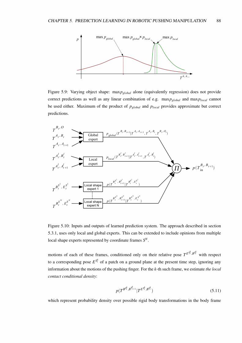
CHAPTER 5. PREDICTION LEARNING IN ROBOTIC PUSHING MANIPULATION 88
max pglobal max plocalmax pglobal× plocal
T Bt , Bt 1
p
Figure 5.9: Varying object shape: maxpglobal alone (equivalently regression) does not provide
correct predictions as well as any linear combination of e.g. maxpglobal and maxplocal cannot
be used either. Maximum of the product of pglobal and plocal provides approximate but correct
predictions.
p T inBt , Bt1
pglobal TBt ,B t1∣T
At ,A t1 , TA t , Bt , T
B t ,Ot
plocal TB tl , B t1
l
∣TAtl , At1
l
,TAtl , Bt
l
pTB tSN , Bt1
SN
∣TBtSN ,E t
SN
Local shapeexpert NT
BtS N , Et
S N
Local shapeexpert 1T
BtS1 , E t
S1
Localexpert
TAtl ,Bt
l
TAtl , At1
l
Globalexpert
TAt , At1
TAt , Bt
TBt ,O
pTB tS1 , Bt1
S1
∣TBtS1 ,E t
S1
Figure 5.10: Inputs and outputs of learned prediction system. The approach described in section
5.3.1, uses only local and global experts. This can be extended to include opinions from multiple
local shape experts represented by coordinate frames SN .
motions of each of these frames, conditioned only on their relative pose T ESkt ,BSk
t with respect
to a corresponding pose ESkt of a patch on a ground plane at the present time step, ignoring any
information about the motions of the pushing finger. For the k-th such frame, we estimate the local
contact conditional density:
p(T BSkt ,BSk
t+1 |T ESkt ,BSk
t ) (5.11)
which represent probability density over possible rigid body transformations in the body frame

CHAPTER 5. PREDICTION LEARNING IN ROBOTIC PUSHING MANIPULATION 89
Object
Environment
BtS1
BtS2
BtS3
TEtS1 , Bt
S1
E tS2
E tS1 E t
S3TEtS3 , Bt
S 3
Figure 5.11: Co-ordinate frames can be attached to an arbitrary number of local shapes, and local
experts can be learned for each of these frames, predicting a distribution of how the frame may
move next, given where it is at the present time step.
of the k-th local contact. The subsequent motion of the object in the inertial frame can now be
predicted as:
maxT
Bt ,Bt+1in
pglobal((T I,Bt )−1T Bt ,Bt+1in T I,Bt |T At ,At+1 ,T At ,Bt ,T Bt ,O)×
plocal((T I,Blt )−1T Bt ,Bt+1
in T I,Blt |T At ,At+1 ,T Al
t ,Blt )×
∏k=1...N
p((T I,BSkt )−1T Bt ,Bt+1
in T I,BSkt |T ESk
t ,BSkt ) (5.12)
5.3.3 Incorporating additional information into the global conditional densityfunction
5.3.3.1 Finger-object contact
Finger Object
EnvironmentTAtl , Bt
l
Btl T
Btl , Bt
TBt ,O
Atl
Bt
O
Figure 5.12: An alternative setup to the one from Figure 5.8 redefines the global conditional
density function using local frame Blt .
The global conditional density function as in Equation 5.6 describes “global” behaviour of all
three interacting objects. From physics we know that contacts between objects are responsible
CHAPTER 5. PREDICTION LEARNING IN ROBOTIC PUSHING MANIPULATION 90
for forces and therefore determine the objects behaviour. Contacts between an object and the
environment can be arbitrarily complex and they are all handled by term T Bt ,O in density 5.6.
However assuming that there is only one contact between the finger and an object one can use more
efficient representation of the global conditional density function, in which term T At ,Bt is replaced
by T Blt ,Bt or equivalently by T Al
t ,Bt (see Figure 5.12). This representation is simpler because it takes
into account only a local shape (Blt or Al
t )-object relation instead of a more complex finger-object
relation. The global conditional density function can be then redefined as:
pglobal(T Bt ,Bt+1 |T At ,At+1 ,T Blt ,Bt ,T Bt ,O) (5.13)
In general it is safer to use more general definition 5.6. However incorporating explicitly
the finger-object contact information might be beneficial in some cases, as it is shown in the
experimental part of this chapter (see Section 5.4.3).
5.3.3.2 Parametrization of objects’ properties
Any additional knowledge about properties of the interacting objects (including the robotic finger
and the environment) which vary in time can also be incorporated into the global conditional
density function. These properties may involve shape variations such as length of an object,
but also properties which cannot be expressed by shape such as friction, restitution, viscosity,
dislocated centre of mass, etc. The global conditional density function can be then expressed as:
pglobal(T Bt ,Bt+1 |T At ,At+1 ,T At ,Bt ,T Bt ,O,X) (5.14)
where X ∈ Rn is some n-dimensional vector describing additional objects’ properties.
Property vector X can also be seen as a predictor context in a similar vein as the movement
context in modular motor learning described in Section 2.5.4, although without autonomous
learning and estimation of X3.
5.3.4 Learning as density estimation
We use non-parametric kernel density estimation in which all learning samples are stored during
learning. The learning samples create a global joint distribution, local joint distribution and N
local contact joint distributions:
{T At ,Bt ,T Bt ,O,T At ,At+1 ,T Bt ,Bt+1} (5.15)
{T Alt ,B
lt ,T At ,At+1 ,T Bt ,Bt+1} (5.16)
{T BSkt ,BSk
t+1 ,T ESkt ,BSk
t } for k = 1 . . .N (5.17)
3Which is an interesting issue to investigate

CHAPTER 5. PREDICTION LEARNING IN ROBOTIC PUSHING MANIPULATION 91
We address 3D rigid bodies, subject to 6-DOF transformations, so that distributions 5.15, 5.16
and 5.17 have 4×6 = 24, 3×6 = 18 and 2×6 = 12 dimensions respectively. During prediction
conditional densities 5.6, 5.7 and 5.11 are created online from learning sample sets (i.e. from the
above joint distributions).
Consider N D-dimensional sample vectors Xi drawn from some unknown distribution. We
would like to find an approximation of this distribution in the form of a density function p(X).
Kernel density methods with Gaussian kernels (see e.g. [Scott and Sain, 2004]) estimates the
density p(X) for any given vector X as a sum of N identical multivariate Gaussian densities centred
on each sample vector Xi:
p(X) = Cnorm ∑i=1...N
exp[−1
2(X−Xi)T C−1(X−Xi)
](5.18)
where a constant Cnorm = [N(2π)D/2|C|1/2]−1 and C is a D×D sample covariance matrix. For
simplicity, we assume that C is diagonal. The above equation can be re-written in a new simpler
form ([Scott and Sain, 2004]):
p(X) =1N ∑
i=1...N
[∏
j=1...DKh j(X
j−X ji )
](5.19)
where Kh j are 1-dimensional Gaussian kernel functions:
Kh j(Xj−X j
i ) =1
(2π)1/2h jexp
[−1
2(X j−X j
i )2
h2j
](5.20)
and D parameters h j are called bandwidth H ≡ (h1, . . . ,hD). The bandwidth H is estimated
from all distribution learning samples using the “multivariate rule-of-thumb” see [Scott and Sain,
2004].
Let us decompose each D-dimensional sample vector Xi into two vectors: K-dimensional Yi
and L-dimensional Zi so that Xi ≡ (Yi,Zi)T and D = K +L. Knowing bandwidth H or equivalently
diagonal covariance matrix C for sample set {Xi} ≡ {(Yi,Zi)T}, we can compute conditional
density p(Z|Y ) for some given vectors Y and Z using the following two step procedure:
1. Find a set of M weighted samples {(Zi,wi)} representing a conditional distribution for
given vector Y , such that Yi which corresponds to Zi lies within some predefined maximum
Mahalanobis distance dmax to vector Y . Mahalanobis distance di between sample vector Yi
and vector Y is defined as:
di = (Y −Yi)T C−1Y (Y −Yi) (5.21)
where diagonal covariance CY is defined as:
C =
[CY 0
0 CZ
](5.22)

CHAPTER 5. PREDICTION LEARNING IN ROBOTIC PUSHING MANIPULATION 92
Weights wi are computed from distance di as:
wi = exp[−di/2] (5.23)
and normalized for all M weights wi. Normalized weight wi can be interpreted as a
probability of generating Yi from a multivariate Gaussian centred at Y with covariance CY .
2. Compute conditional probability density p(Z|Y ) as:
p(Z|Y ) = ∑i=1...M
wi exp[−1
2(Z−Zi)T C−1
Z (Z−Zi)]
(5.24)
For simplicity, the density product 5.10 is maximized using the differential evolution
optimization algorithm [Storn and Price, 1997]4 which is described in Appendix C. This requires
the ability to evaluate and sample from each distribution comprising product 5.10.
All conditional distributions are represented as a weighted set of samples {(Zi,wi)}.Computation of a probability density for some given vector Z is realized as in Equation 5.24.
Sampling consists of a two step procedure:
1. Choose vector Zi from a set of samples {(Zi,wi)} using an importance sampling algorithm
with importance weights wi ([Bishop, 2006]).
2. Sample from a multivariate Gaussian centred at Zi with covariance CZ .
5.4 Results
5.4.1 Introduction
5.4.1.1 Experimental setup
We have tested the introduced prediction algorithms in simulation experiments using the PhysX
physics engine [PhysX, 2009]. We also performed real experiments using a 5-axis Katana robotic
manipulator [Neuronics AG, 2004] equipped with a single rigid finger and where we capture the
motion of the polyflap using a vision model-based tracking system [Morwald et al., 2009]. We
use both because simulation experiments are useful in that they can provide large amounts of test
data with perfectly known ground-truth, but they do not necessary corresponds to reality. This is
the reason we tested the ability of our approach to predict motions of a real object being pushed
by a real robot.
They are used to study three phenomena:
4In the optimal scenario the mean shift method [Comaniciu and Meer, 2002] should be used here.

CHAPTER 5. PREDICTION LEARNING IN ROBOTIC PUSHING MANIPULATION 93
Generalization with respect to actions performed. We study the generalisation ability of vari-
ous predictors when the actions vary from those in the training set. We vary the actions in
two ways. In experiment 1 we study interpolative generalisation where actions are novel
but drawn from the same Euclidean space as the training set. We then study extrapolative
generalisation (Experiment 2 and 3) by drawing actions from a space which sits outside that
from which the training actions were drawn.
Generalization with respect to shape. We study the generalisation ability of various predictors
when presented with novel shape. We train the predictors on a simple fixed polyflap shape,
and then test on novel polyflap (Experiment 4), and on a box object (Experiment 5). This is
extrapolative generalisation with respect to shape because the test set lies outside the set of
shapes used for training. In Experiment 6 we train a varying set of shapes (all polyflaps) and
then we test generalisation with respect to shapes which are interpolations of the training
shapes.
Convergence. In Experiment 1 we also study the rate of convergence on the test set as a function
of the number of training pushes.
All the above prediction problems have been addressed in simulation environments in Section 5.4.2
and Section 5.4.3. Real experiments are presented in Section 5.4.4 addressing only the first
prediction problem mostly due to limitations of the vision tracker.
In each test scenario, we compare the performance of three approaches (further called
predictors):
1. A multiple expert method with global, local and local shape experts (see Section 5.3).
2. A single global expert method as a ground-truth comparison to the multiple expert method
(see Section 5.2).
3. A state of the art regression method described in Section 5.4.1.5.
Multiple experimental trials were performed, in which a robotic arm equipped with a finger
performs a random pushing movement of length approximately 25 cm towards an object placed at
a random initial pose (Figure 5.26). In each experiment data samples are stored over a series of
such random trials. Each trial lasts 10 seconds, while data samples are stored every 1/15th of a
second.
We performed 10-fold cross-validation where at the beginning of each experiment all the trials
are randomly partitioned into 10 subsets. Prediction was then subsequently performed (10 times)
on each single subset, while learning was always performed on the remaining 9 subsets of these
trials. All the results were then averaged to produce a single estimation.

CHAPTER 5. PREDICTION LEARNING IN ROBOTIC PUSHING MANIPULATION 94
5.4.1.2 Model selection
In model selection we are concerned with identifying a model that is likely to generalise well
to unseen data. In particular we need to optimise generalisation performance with respect to
model complexity and the hyper-parameters of the learning algorithms used. For a single KDE
learner we used one hyper-parameter which equally scales all the bandwidth parameters h j from
Equation 5.20. For LWPR there are also a small number of hyper-parameters which are described
in details in [Klanke et al., 2008].
In this initial study we have not looked at how generalisation performance varies with hyper-
parameters. However for the parameters we have performed 10-fold cross validation in all our
experiments. This gives us limited evidence that while we have not optimized with respect to the
hyper-parameters, some generalisation is possible.
In practice however, we note that the extrapolative kind of generalisation we ask our learners
to perform is quite unusual in that generalisation studies normally assume that the test set is drawn
independently from the same density over the input space as the training set (the i.i.d. assumption).
In the case of extrapolative generalisation with respect to both shape and action direction our
problem is rather different from (and harder than) this.
5.4.1.3 Performance measure
In all experiments, we take the output of either a physics simulator or the tracked pose of a
real object to be ground-truth, and compare it against predictions forecast by the learned system.
Prediction performance is evaluated as follows.
At any particular time step, t, a large number, N, of randomly chosen points p1,tn , where
n = 1 . . .N, are rigidly attached to an object at the ground-truth pose, and the corresponding points
p2,tn to an object at the predicted pose (see Figure 5.13). At time step t, an average error Et can
now be defined as the mean of displacements between points on the object at the predicted pose
and points on the object at the ground-truth pose:
Et =1N ∑
n=1...N|p2,t
n − p1,tn | (5.25)
Note that for each robotic push action, we predict approximately 150 consecutive steps into
the future, with no recursive filtering or corrector steps, hence it is expected that errors will grow
with range from the initial object pose. We therefore find it more meaningful to normalize all
errors with respect to an “average range”, Rt , of the object from its starting position, defined as:
Rt =1N ∑
n=1...N|p1,t
n − p1,0n | (5.26)
For a test data set, consisting of K robotic pushes, each of which breaks down into many
consecutive predictions over T time steps, we can now define an normalized average error:
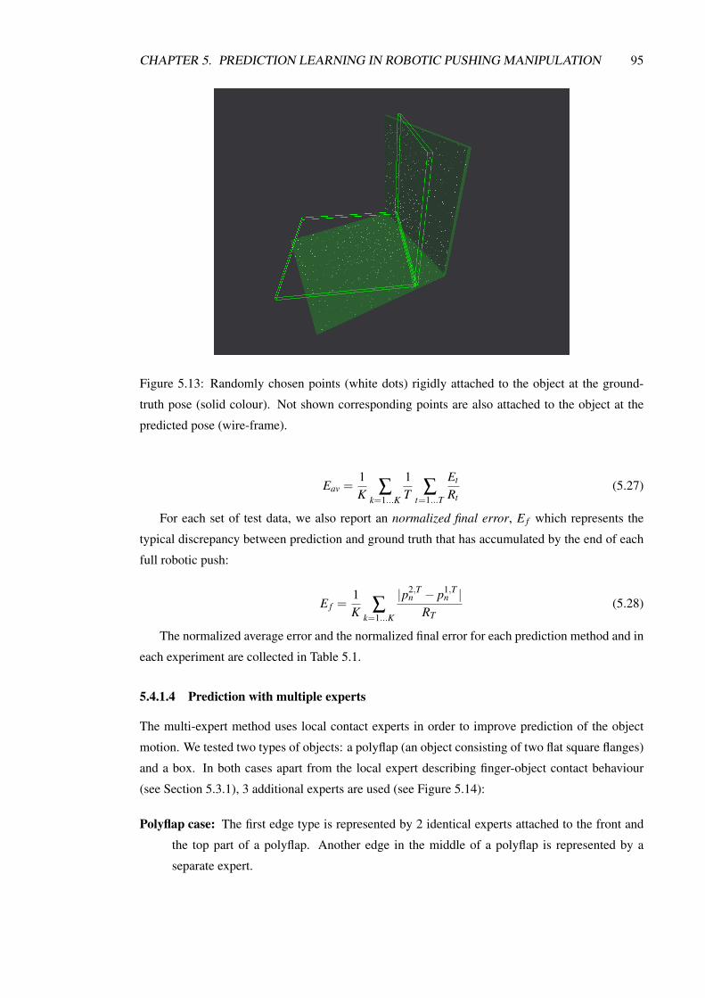
CHAPTER 5. PREDICTION LEARNING IN ROBOTIC PUSHING MANIPULATION 95
Figure 5.13: Randomly chosen points (white dots) rigidly attached to the object at the ground-
truth pose (solid colour). Not shown corresponding points are also attached to the object at the
predicted pose (wire-frame).
Eav =1K ∑
k=1...K
1T ∑
t=1...T
Et
Rt(5.27)
For each set of test data, we also report an normalized final error, E f which represents the
typical discrepancy between prediction and ground truth that has accumulated by the end of each
full robotic push:
E f =1K ∑
k=1...K
|p2,Tn − p1,T
n |RT
(5.28)
The normalized average error and the normalized final error for each prediction method and in
each experiment are collected in Table 5.1.
5.4.1.4 Prediction with multiple experts
The multi-expert method uses local contact experts in order to improve prediction of the object
motion. We tested two types of objects: a polyflap (an object consisting of two flat square flanges)
and a box. In both cases apart from the local expert describing finger-object contact behaviour
(see Section 5.3.1), 3 additional experts are used (see Figure 5.14):
Polyflap case: The first edge type is represented by 2 identical experts attached to the front and
the top part of a polyflap. Another edge in the middle of a polyflap is represented by a
separate expert.

CHAPTER 5. PREDICTION LEARNING IN ROBOTIC PUSHING MANIPULATION 96
Figure 5.14: In the polyflap case (top panel) the first edge type is represented by 2 identical experts
attached to the front and the top part of a polyflap (small white surface patches with reference
frames). A separate expert represents the edge in the middle of a polyflap. In the box case (bottom
panel) there are 3 identical experts attached to 3 different parts of a box.
Box case: All edges are assumed to be of the same type therefore all 3 experts are identical
although attached to different parts of a box.
If two or more experts are identical they all share the same joint distribution during learning and
prediction.
The parameter scaling the bandwidth of distributions was tuned by hand on a test set from
Experiment 1 and kept constant throughout all the experiments.

CHAPTER 5. PREDICTION LEARNING IN ROBOTIC PUSHING MANIPULATION 97
5.4.1.5 Prediction by regression
To provide a comparison with a more conventional function approximation approach, we
employed a powerful regression algorithm – Locally Weighted Projection Regression (LWPR)
[Vijayakumar et al., 2005]. LWPR is an online algorithm that uses dimensionality reduction to
learn non-linear mappings from high-dimensional input spaces, by using a set of local models.
Thus we attempted to predict the rigid body motion of an object (frame B) subjected to a push
from a finger (frame A), by learning a non-linear function G. The function G is analogous to the
global expert of the probabilistic approach in section 5.3.
The input domain for the regression was an 18 dimensional vector formed by the concatenation
of three 6-DOF transformations, where each transformation was represented as a displacement and
three Euler angles. The 6 dimensional output vector was simply the change in pose of object B, so
that
G : T At ,Bt ,T Bt ,O,T At ,At+1 → T Bt ,Bt+1 . (5.29)
The hyper-parameters for LWPR were tuned by hand on a test set from Experiment 1. The
(diagonal) distance metric D was held fixed, and initialized so that the local model receptive fields
were small for the finger-object interaction T At ,Bt , and large for the other input dimensions.
The regression scheme was implemented using the LWPR software library [Klanke et al.,
2008].
5.4.2 Generalization to predict motions from novel actions
5.4.2.1 Interpolative generalization of push directions
In Experiment 1 with a virtual robot, pushes with random directions were applied to a polyflap of
a fixed shape. Some pushes were randomized about a direction approximately orthogonal to the
contacted polyflap face, and some were randomized about a direction at an oblique angle. Both
orthogonal and oblique pushes were used during training, new examples of each class of push
direction were then used in testing. We consider this a test of “interpolative” generalization, in that,
although the test pushes are different from any particular push in the training set, the directions of
the test pushes lie within a space of directions that are reasonably spanned by training examples.
Figure 5.15 shows how the average and final prediction error decreases with increased
number of trials used in learning for four tested prediction methods. The density-based methods
outperforms LWPR regression in each case. It is also clear that using the introduced prediction
error in the interpolative generalization case, multiple expert methods do not show any advantage
over the single global expert method if they are learned on the same data.

CHAPTER 5. PREDICTION LEARNING IN ROBOTIC PUSHING MANIPULATION 98
10 100 10000.000
0.020
0.040
0.060
0.080
0.100
0.120
number of trials
norm
aliz
ed a
vera
ge e
rror
globalglobal+localglobal+local+shapesLWPR
10 100 10000.000
0.050
0.100
0.150
0.200
0.250
0.300
number of trials
norm
aliz
ed fi
nal e
rror
globalglobal+localglobal+local+shapesLWPR
Figure 5.15: Experiment 1. Decrease in average (top) and final (bottom) prediction errors with
increased number of trials used in learning, for four different prediction method.
5.4.2.2 Extrapolative generalization of push directions
In Experiment 2, only the orthogonal type of pushes were used during training, pushes being
applied to both the front and rear surfaces of a polyflap. However, only the oblique type pushes
were used during testing. We consider this to be a test of “extrapolative” generalization, in that the
push directions used in testing are all qualitatively different from those used in training - the test
push directions do not lie in the same region of data covered by the training examples.
The regression method makes the smallest error mostly because it manages to differentiate
between tipping/toppling and forward pushing as it is shown in Figure 5.16. The single expert
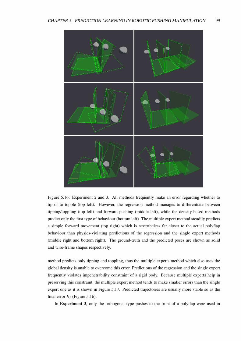
CHAPTER 5. PREDICTION LEARNING IN ROBOTIC PUSHING MANIPULATION 99
Figure 5.16: Experiment 2 and 3. All methods frequently make an error regarding whether to
tip or to topple (top left). However, the regression method manages to differentiate between
tipping/toppling (top left) and forward pushing (middle left), while the density-based methods
predict only the first type of behaviour (bottom left). The multiple expert method steadily predicts
a simple forward movement (top right) which is nevertheless far closer to the actual polyflap
behaviour than physics-violating predictions of the regression and the single expert methods
(middle right and bottom right). The ground-truth and the predicted poses are shown as solid
and wire-frame shapes respectively.
method predicts only tipping and toppling, thus the multiple experts method which also uses the
global density is unable to overcome this error. Predictions of the regression and the single expert
frequently violates impenetrability constraint of a rigid body. Because multiple experts help in
preserving this constraint, the multiple expert method tends to make smaller errors than the single
expert one as it is shown in Figure 5.17. Predicted trajectories are usually more stable so as the
final error E f (Figure 5.16).
In Experiment 3, only the orthogonal type pushes to the front of a polyflap were used in

CHAPTER 5. PREDICTION LEARNING IN ROBOTIC PUSHING MANIPULATION 100
oblique pushes back pushes0.000
0.020
0.040
0.060
0.080
0.100
0.120
0.140
0.160
norm
aliz
ed a
vera
ge e
rror
globalglobal+local+shapesLWPR
oblique pushes back pushes0.000
0.050
0.100
0.150
0.200
0.250
0.300
0.350
0.400
norm
aliz
ed fi
nal e
rror
globalglobal+local+shapesLWPR
Figure 5.17: Experiment 2 and 3. Extrapolative action generalization errors for oblique pushes
and back pushes.
training, along with oblique type pushes. In contrast, the system was tasked to make predictions
for orthogonal type pushes applied to the back of a polyflap.
The regression method and the single expert method fail to predict the polyflap behaviour
(see Figure 5.17). Although the multiple expert method steadily predicts a simple forward
movement of a polyflap it does not violate physics and roughly corresponds to the actual behaviour
(Figure 5.16).
5.4.3 Generalization to objects with novel shapes
5.4.3.1 Extrapolative generalization to novel shapes
In Experiment 4, training data featured only an ordinary polyflap constructed from two square
faces joined at right angles. However, predictions were then made for test data in which the
geometry of the polyflaps varied randomly in several ways, see Figure 5.18. Variations included:
the angle at which the two rectangular flanges of the polyflap were connected; the width of each
rectangular flange; the transverse offset of one flange with respect to the other. We again consider
this to be an example of “extrapolative” generalization, in that the different kinds of test shape are
not spanned by the single shape used during training.
All prediction methods performed well with a slight advantage of the multiple expert method
(Figure 5.20). A typical error is related to inability to differentiate between tipping/toppling
behaviour of a polyflap (Figure 5.18).
In Experiment 5, the system is trained on a polyflap, but in testing it is required to predict the
motions of a box shaped object. This is a severe test of “extrapolative” generalization.
Similarly as in Experiment 3 the multiple expert method predicts a simple forward movement
of a box without violating physics (Figure 5.18). In contrast the single expert and the regression
methods constantly violate physics although they predict some sort of forward movement. As
in Experiment 2 the regression method frequently manages to predict qualitative character of a
movement such as rotation or toppling.

CHAPTER 5. PREDICTION LEARNING IN ROBOTIC PUSHING MANIPULATION 101
Figure 5.18: Experiment 4 and 5. An example of shape variation and tipping/toppling error (top
left). The multiple expert method trained on a polyflap predicts a simple forward movement of
a box (top right). In contrast, the single expert method (bottom left) and the regression method
(bottom right) constantly violate impenetrability constraints. The ground-truth and the predicted
poses are shown as solid and wire-frame shapes respectively.
5.4.3.2 Interpolative generalization to novel shapes
In Experiment 6, all training and testing data involve polyflaps constructed from two square
flanges. Shape variation consists in varying the angle at which the two square flanges are connected
along a common edge (see Figure 5.19). The shapes used for training are different from those
encountered by the predictors during testing, however we consider this a form of “interpolative”
generalization task, in that the test and training shapes are qualitatively similar and the range of
test shapes can be considered to be spanned by the range of training examples.
This experiment is informative, in that it reveals limitations of the regression method as well
as the single expert method. Since the regression technique does not encode information about
the object shape variability, it is difficult for it to generalize in situations where small changes in
shape can cause significant and qualitative changes in the resulting motion, even when the robotic
push is the same. For example, see Figure 5.19, when subjected to a downwards push, the angle
at which the polyflap flanges are joined, determines whether it will be pushed towards the left or
towards the right. In contrast to regression, the product of experts techniques cope much better
with this kind of shape generalization.

CHAPTER 5. PREDICTION LEARNING IN ROBOTIC PUSHING MANIPULATION 102
Figure 5.19: Experiment 6 reveals limitations of the single expert and the regression methods
which fail to predict the motion of a polyflap when subjected to a downward push (bottom panel).
Both methods constantly predict the same motion of a polyflap. The multiple expert method can
cope well with this kind of shape variations (top panel). The ground-truth and the predicted poses
are shown as solid and wire-frame shapes respectively.
variable polyflap box downward pushes0.000
0.020
0.040
0.060
0.080
0.100
0.120
0.140
0.160
0.180
norm
aliz
ed a
vera
ge e
rror
globalglobal+local+shapesLWPR
variable polyflap box downward pushes0.000
0.050
0.100
0.150
0.200
0.250
0.300
0.350
0.400
0.450
norm
aliz
ed fi
nal e
rror
globalglobal+local+shapesLWPR
Figure 5.20: Experiment 4, 5 and 6. Shape generalization errors for a variable polyflap
(Experiment 4), a box (Experiment 5) and downward pushes (Experiment 6).
5.4.3.3 Incorporating additional shape information into the global expert
As we could see in Experiment 6, the single expert method failed because the corresponding
conditional density function 5.6 is not capable to determine whether a polyflap is pushed towards
the left or towards the right (Figure 5.19). We extended Experiment 6 by two predicting methods
to test if introducing additional information about contacts and about shape variability can improve
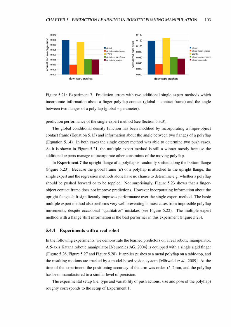
CHAPTER 5. PREDICTION LEARNING IN ROBOTIC PUSHING MANIPULATION 103
0.000
0.005
0.010
0.015
0.020
0.025
0.030
0.035
0.040
downward pushes
norm
aliz
ed a
vera
ge e
rror
globalglobal+local+shapesLWPRglobal+contact f rameglobal+parameter
0.000
0.020
0.040
0.060
0.080
0.100
0.120
0.140
downward pushes
norm
aliz
ed fi
nal e
rror
globalglobal+local+shapesLWPRglobal+contact f rameglobal+parameter
Figure 5.21: Experiment 7. Prediction errors with two additional single expert methods which
incorporate information about a finger-polyflap contact (global + contact frame) and the angle
between two flanges of a polyflap (global + parameter).
prediction performance of the single expert method (see Section 5.3.3).
The global conditional density function has been modified by incorporating a finger-object
contact frame (Equation 5.13) and information about the angle between two flanges of a polyflap
(Equation 5.14). In both cases the single expert method was able to determine two push cases.
As it is shown in Figure 5.21, the multiple expert method is still a winner mostly because the
additional experts manage to incorporate other constraints of the moving polyflap.
In Experiment 7 the upright flange of a polyflap is randomly shifted along the bottom flange
(Figure 5.23). Because the global frame (B) of a polyflap is attached to the upright flange, the
single expert and the regression methods alone have no chance to determine e.g. whether a polyflap
should be pushed forward or to be toppled. Not surprisingly, Figure 5.23 shows that a finger-
object contact frame does not improve predictions. However incorporating information about the
upright flange shift significantly improves performance over the single expert method. The basic
multiple expert method also performs very well preventing in most cases from impossible polyflap
movements, despite occasional “qualitative” mistakes (see Figure 5.22). The multiple expert
method with a flange shift information is the best performer in this experiment (Figure 5.23).
5.4.4 Experiments with a real robot
In the following experiments, we demonstrate the learned predictors on a real robotic manipulator.
A 5-axis Katana robotic manipulator [Neuronics AG, 2004] is equipped with a single rigid finger
(Figure 5.26, Figure 5.27 and Figure 5.28). It applies pushes to a metal polyflap on a table-top, and
the resulting motions are tracked by a model-based vision system [Morwald et al., 2009]. At the
time of the experiment, the positioning accuracy of the arm was order +/- 2mm, and the polyflap
has been manufactured to a similar level of precision.
The experimental setup (i.e. type and variability of push actions, size and pose of the polyflap)
roughly corresponds to the setup of Experiment 1.

CHAPTER 5. PREDICTION LEARNING IN ROBOTIC PUSHING MANIPULATION 104
Figure 5.22: Experiment 7. The basic single expert method frequently generates physically
impossible movements (left panel). However, the basic multiple expert method performs very
well preventing from impossible polyflap movements, despite occasional “qualitative” mistakes
(right panel).
0.000
0.010
0.020
0.030
0.040
0.050
0.060
0.070
shifted flange
norm
aliz
ed a
vera
ge e
rror
globalglobal+local+shapesLWPRglobal+contact f rameglobal+parameterglobal+local+shapes+parameter
0.0000.0200.0400.0600.0800.1000.1200.1400.1600.1800.200
shifted flange
norm
aliz
ed fi
nal e
rror
globalglobal+local+shapesLWPRglobal+contact f rameglobal+parameterglobal+local+shapes+parameter
Figure 5.23: Experiment 7. Prediction errors with three additional methods.
5.4.4.1 Real experimental learning data
In Experiment 8 we have trained the system on 9, 90 and 900 pushes of a real robot. We
evaluated the performance of the multiple and the single expert methods and the regression
method. Figure 5.24 shows that the average and final prediction error decreases with increased
number of trials used in learning for all tested prediction methods. All density-based methods
performed reasonably well learned with even so little as 9 example pushes. The multiple expert
method performs particularly well with 90 learning trials where local experts successfully prevent

CHAPTER 5. PREDICTION LEARNING IN ROBOTIC PUSHING MANIPULATION 105
9 90 9000.000
0.050
0.100
0.150
0.200
0.250
0.300
number of trials
norm
aliz
ed a
vera
ge e
rror
globalglobal+local+shapesLWPR
9 90 9000.0000.0500.1000.1500.2000.2500.3000.3500.4000.4500.500
number of trials
norm
aliz
ed fi
nal e
rror
globalglobal+local+shapesLWPR
Figure 5.24: Experiment 8 with a real robot. Decrease in average (top) and final (bottom)
prediction errors with increased number of trials used in learning, for three different prediction
method.
from violating impenetrability constraints as it is frequently the case with the other tested methods.
However, the multiple expert method does not significantly improve its performance with 900
learning trials. Also, none of the tested method achieves the level of performance from Experiment
1. One of the reasons for this is that the vision tracker was not able to provide a sequence of
tracked object poses of pose-independent quality. We found that tipping and toppling movements
were particularly difficult to track.

CHAPTER 5. PREDICTION LEARNING IN ROBOTIC PUSHING MANIPULATION 106
global global+local+shapes LWPR0.000
0.050
0.100
0.150
0.200
0.250
norm
aliz
ed a
vera
ge e
rror
real learning datavirtual learning data
global global+local+shapes LWPR0.000
0.100
0.200
0.300
0.400
0.500
norm
aliz
ed fi
nal e
rror
real learning datavirtual learning data
Figure 5.25: Experiment 8 and 9. Predictors trained in a simulation are unable to match predictors
trained in the real experiment.
5.4.4.2 Virtual experimental learning data
In Experiment 9, we have trained the system on 900 simulated robot pushes which correspond
to those from Experiment 8. Parameters of a simulation were tuned by hand to match the real
system. Then we attempted to predict the motion of the real polyflap when it is pushed by the
real robot. Figure 5.26 and Figure 5.27 show two distinct qualitative behaviours where predictions
are convincingly accurate. Figure 5.28 shows that the predicted behaviour is physically plausible
and qualitatively correct, however a quantitative error has resulted from learning on simulated
data rather than real test data: while the system has correctly learned to predict the motion of
the polyflap within the physics simulator, the physics simulator does not accurately model the
frictional interactions of the real world, leading to a discrepancy between the predicted and real
polyflap motions in this case.
Figure 5.25 presents a comparison of prediction methods learned in a real experiment
(Experiment 8) and in a virtual experiment (Experiment 9), all with 900 learning trials. Clearly,
predictors trained in a simulation are unable to match predictors trained in a real experiment
despite some problems with the polyflap pose tracking.
5.5 Summary
In this chapter we have introduced an array of methods for learning to predict the motions
of objects during robotic manipulation tasks, that are able to encode physics information
without explicitly representing physics knowledge. We show that various geometric relations
between parts of objects can be represented as statistically independent shape/contact experts -
distributions, when used in products of experts allow us to generalize over shape and applied
actions, as well as to effectively learn in high dimensional spaces.
We have also presented an alternative prediction system based on a state of the art regression
method. The regression method and the single expert method show some advantage only when

CHAPTER 5. PREDICTION LEARNING IN ROBOTIC PUSHING MANIPULATION 107
Figure 5.26: Experiment 8 and 9. Prediction (green wire frame) for a real experiment (red wire
frame denotes visual tracking). The polyflap tips forward before rocking back to its starting
position. Predictions were generated by the multiple expert method.
Figure 5.27: Experiment 8 and 9. Prediction (green wire frame) for a real experiment (red wire
frame denotes visual tracking). The polyflap tips forward and then topples over. Predictions were
generated by the multiple expert method.

CHAPTER 5. PREDICTION LEARNING IN ROBOTIC PUSHING MANIPULATION 108
Figure 5.28: Experiment 8 and 9. Prediction (green wire frame) for a real experiment (red wire
frame denotes visual tracking). Blue wire frame denotes prediction of a physics simulator. Note
that the learned statistical predictor has correctly learned to replicate the physics simulator data
that it was trained on, but fails to properly predict the real object motion because the physics
simulator training data does not always correspond well with reality. Predictions were generated
by the multiple expert method.
there is low variation in shape and action, but its performance deteriorates where shape variation
occurs that substantially affects object behaviour. In contrast, the multiple experts approaches
extrapolate comparatively well in such situations.
Furthermore, we have shown that the introduced prediction methods can be successfully used
to learn to predict from real experiments with a small number of examples. All methods trained
in a real experiment provide substantially better predictions than methods trained in a simulation.
The multiple experts method shows the best performance of all other methods, especially when
trained with a small number of example pushes.
Future work will investigate (for more details see Chapter 7):
• Product of experts can incorporate observations during prediction using recursive Bayesian
filter.
• Autonomous selection and construction of experts could allow to select and also construct
experts in an autonomous way to provide the best prediction results.

CHAPTER 5. PREDICTION LEARNING IN ROBOTIC PUSHING MANIPULATION 109
• Shape invariant experts constructed using information about contacts and the centre of mass
of an object can be common for a large set of objects.
• Learning to predict in compliant manipulation and grasping which involves motor torques
rather than a kinematic type of actions.
• Applying products of experts in inverse models.
• Combining forward and inverse models in modular motor learning.

CHAPTER 5. PREDICTION LEARNING IN ROBOTIC PUSHING MANIPULATION 110
Experiment Prediction method Eav E f
1 (1000 trials) single expert (global) 0.0203 0.0638
multiple experts (global+local) 0.0226 0.0712
multiple experts (global+local+shapes) 0.0227 0.0716
regression (LWPR) 0.0426 0.1326
2 single expert (global) 0.0836 0.2816
multiple experts (global+local+shapes) 0.0783 0.2266
regression (LWPR) 0.0607 0.1893
3 single expert (global) 0.1503 0.3669
multiple experts (global+local+shapes) 0.0141 0.0393
regression (LWPR) 0.1392 0.3600
4 single expert (global) 0.0537 0.1696
multiple experts (global+local+shapes) 0.0463 0.1537
regression (LWPR) 0.0536 0.1636
5 single expert (global) 0.1666 0.4286
multiple experts (global+local+shapes) 0.1114 0.2722
regression (LWPR) 0.1175 0.2332
6 single expert (global) 0.0345 0.1188
multiple experts (global+local+shapes) 0.0098 0.0359
regression (LWPR) 0.0328 0.1287
single expert (global+contact frame) 0.0157 0.0607
single expert (global+parameter) 0.0151 0.0558
7 single expert (global) 0.0578 0.1688
multiple experts (global+local+shapes) 0.0338 0.0867
regression (LWPR) 0.0557 0.1815
single expert (global+contact frame) 0.0575 0.1596
single expert (global+parameter) 0.0301 0.0799
multiple experts (global+local+shapes+parameter) 0.0286 0.0697
8 (900 trials) single expert (global) 0.0794 0.1424
multiple experts (global+local+shapes) 0.0781 0.1460
regression (LWPR) 0.1043 0.2026
9 single expert (global) 0.1888 0.3700
multiple experts (global+local+shapes) 0.1887 0.3721
regression (LWPR) 0.1675 0.3281
Table 5.1: Comparative performance of tested prediction methods.

Chapter 6
A simplified physics approach toprediction
The previous chapter presented a set of methods for learning to predict the behaviour of objects
in simple robotic manipulation tasks. The methods incorporate information about objects’ shapes
and other physical properties in terms of distributions. The local distributions encode information
about the behaviour of objects’ local shape parts during interactions and can be shared among
many objects. However, the global distribution is unique to a particular object or object category,
therefore the generalization capabilities of such global distributions are limited, in particular with
respect to objects of different shapes.
This chapter introduces a simplified physics approach as an alternative method for improving
predictions in the case of limited information about the manipulated object. Experimental results
confirm that this simple method can be successfully used in prediction.
The chapter consists of the following sections:
• Section 6.1 introduces the principle of minimum energy which underlies the simplified
physics approach.
• Section 6.2 describes implementation details of the simplified physics approach.
• Section 6.3 presents the results of experiments which compare the simplified physics
predictions with methods introduced in the previous chapter.
• Section 6.4 summarizes the chapter and briefly discusses future work on the simplified
physics approach.
6.1 Principle of minimum energy
A simplified physics approach is an alternative method for predicting the motion of an object
subjected to pushing action. The approach relies on the principle of minimum energy known from
111

CHAPTER 6. A SIMPLIFIED PHYSICS APPROACH TO PREDICTION 112
thermodynamics as a consequence the second law of thermodynamics applied to closed systems.
The principle of minimum energy states that the total energy of a closed system decreases and
reaches a local minimum value at equilibrium, where a closed system is a system with fixed
entropy and other parameters such as volume or mass, but which can exchange energy with other
connected systems [Landau and Lifshitz, 1980].
A system consisting of a robot, an object and a ground plane can also be considered as a closed
system1. From the principle of minimum energy we know that the total energy of our system must
reach a local minimum for a given amount of work introduced to the system. Each movement of
a robotic finger, if it touches an object, produces some amount of work, which in the prediction
scenario is unknown because the corresponding movement of the object is unknown. However,
this movement can be computed by searching for such movements which minimize the produced
amount of work, given known physical properties of the system.
A simplified physics approach uses a very simple model of physical interactions (see also
Chapter 3), which can be split into the physical phenomena and the corresponding work done by
moving objects as follows:
1. Mass via work done by accelerating a given object.
2. Gravity force via work done while moving in a given potential field.
3. Friction via work done by two objects in contact moving in tangential direction. It is
the simplest case of Coulomb’s law of sliding friction with dynamic friction only (see
Section 3.2.2.3).
4. Restitution via work done by two objects in contact moving in directions normal to the
contacting surfaces.
6.2 Implementation
6.2.1 Finding a trajectory at equilibrium
The simplified physics approach represents the object body by a set of N “volumetric” particles
vit with index i at discrete time step t randomly generated at time step t = 0 and then rigidly
attached to the object throughout all prediction time steps (see Figure 6.1). Trajectory of an object
is approximated by a sequence of rigid body transformations q which are found by solving a
problem of minimizing the energy function E(q) at each time step t = 2, . . . ,T :
minq
E(q, t) (6.1)
Energy function E(q) consists of four work type-specific functions which correspond to four ways
of producing work as described in the previous section:
1Only by analogy.

CHAPTER 6. A SIMPLIFIED PHYSICS APPROACH TO PREDICTION 113
Figure 6.1: A set of “volumetric” particles (yellow dots) representing the object body (green solid
shape).
E(q, t) = Ea(q, t)+Egi (q, t)+E f
i (q, t)+Eri (q, t) (6.2)
where each work function computes work during movement generated by q as follows2:
Ea(q, t) = Ca‖N
∑i=1
(qvit−1−2vi
t−1 + vit−2)‖ (6.3)
Egi (q, t) =−Cg
N
∑i=1
G · (qvit−1− vi
t−1) (6.4)
E fi (q, t) = C f ∑
i∈Vf
‖qvit−1− vi
t−1‖ (6.5)
Eri (q, t) = Cr ∑
i∈Vr
di(qvit−1) (6.6)
where C∗ ∈ R+ are work type-specific constants, G ∈ R3 is the gravity vector, Vf is an index set
of all particles which are in contact with the ground plane, Vr is an index set of all particles which
penetrate a robotic finger or the ground plane with the corresponding penetration depth di.
Transformation q which minimizes E(q) can be computed using e.g. a differential evolution
optimization algorithm described in Appendix C.
6.2.2 Probability density over trajectories
Energies E(q) can be transformed into a probability density function over possible transformations
q by using a Boltzmann distribution [Landau and Lifshitz, 1980]:2Work functions are only a crude approximation of real physical phenomena and do not even preserve physical
units.

CHAPTER 6. A SIMPLIFIED PHYSICS APPROACH TO PREDICTION 114
pBoltzmann(E(q)) =exp(−E(q)
kT
)Z(T )
(6.7)
where k is Boltzmann constant and T is temperature. Z(T ) is a partition function (a normalization
constant) which for a given temperature can be computed from:
Z(T ) = ∑q
exp(−E(q)
kT
)(6.8)
A basic prediction scenario requires computation of only the most likely trajectory, therefore
normalization constant Z(T ) need not to be estimated and can be assumed a non-zero constant.
Importantly, the modelled system consisting of an object and a robotic arm is a macroscopic
system, therefore laws thermodynamics cannot be applied directly. Consequently, the temperature
in 6.7 cannot be interpreted as temperature in thermodynamics.
pBoltzmann(E(q)) can be used as an approximation of the global conditional density function
given by Equation 5.6 and it can be combined in a product with other experts as was discussed in
Chapter 5. The global conditional density function can be replaced with pBoltzmann(E(q)) so that
Equation 5.12 now becomes:
maxT
Bt ,Bt+1in
pBoltzmann(E(T Bt ,Bt+1in ))×
plocal((T I,Blt )−1T Bt ,Bt+1
in T I,Blt |T At ,At+1 ,T Al
t ,Blt )×
∏k=1...N
p((T I,BSkt )−1T Bt ,Bt+1
in T I,BSkt |T ESk
t ,BSkt ) (6.9)
where symbol T stands for a rigid body transformation. All predictions can be now computed
using the same procedure as described in Section 5.3.4, i.e. by minimizing product 6.9.
pBoltzmann(E(q)) depends on several constants which have to be estimated for a particular sys-
tem, but crucially it also depends on temperature T . When temperature T→∞, pBoltzmann(E(q))→1 for any transformation q, consequently pBoltzmann(E(q)) has no influence on a result of the max-
imization procedure 6.9. On the other hand, when temperature T → 0, pBoltzmann(E(q)) becomes
very rugged, likely with a single peak only, so that the other factors in the product 6.9 have no
impact on the maximization result3.
6.3 Results
6.3.1 Overview
The experimental setup is identical to that described in Section 5.4. Product 6.9 involves the same
local shape experts as in the multiple expert method which have to be learned prior to prediction.
3This temperature property of pBoltzmann(E(q)) also enables to control the process of learning of the global expert.

CHAPTER 6. A SIMPLIFIED PHYSICS APPROACH TO PREDICTION 115
For comparison we present the results of the simplified physics approach alongside the results
already shown in Chapter 5, for the various learned predictors. The normalized average error and
the normalized final error for each experiment are collected in Table 6.1.
6.3.2 Performance of a simplified physics approach
global global+local+shapes LWPR physics low T0,000
0,050
0,100
0,150
0,200
0,250
norm
aliz
ed a
vera
ge e
rror
real learning datavirtual learning data
+local+shapesglobal global+local+shapes LWPR physics low T
0,000
0,050
0,100
0,150
0,200
0,250
0,300
0,350
0,400
0,450
norm
aliz
ed fi
nal e
rror
real learning datavirtual learning data
+local+shapes
Figure 6.2: Prediction errors of a simplified physics approach compared to prediction errors of
learning methods from Experiment 8 (“virtual learning data”) and Experiment 9 (“real learning
data”).
In order to test the performance of a simplified physics approach, we have repeated
Experiments 8 and 9 (see Section 5.4.4) using the simplified physics predictor combined with
learned local experts as in Equation 6.9 for low temperature T (“physics low T+local+shapes”).
Note that the low temperature means that the physics predictor dominates over contributions from
the local and shape predictors with which it is combined. Figure 6.2 shows the performance of
simplified physics versus various kinds of learned prediction methods.
Bars labelled “virtual learning data” represent prediction errors for predictors trained on data
from a physics simulator and then tested on real data (Experiment 8). Bars labelled “real learning
data” represent prediction errors for predictors both trained and tested on real data (Experiment
9). This comparison is important, because it reveals that, in the absence of data with which to train
a global expert, it is better to use a simplified physics predictor than to attempt to use a physics
simulator - the simplified physics provides better predictions than those which can be achieved by
using a physics simulator to train a predictor.
It is observed that the learned global expert (when combined with local experts) somewhat
outperforms the simplified physics predictor. However, the simplified physics is of broadly
comparable performance, but does not need prior observations of a particular object in order for
training.
Note that in these proof of principle experiments, parameters of the simplified physics
predictor (constants C∗ from Equation 6.6) were manually tuned to match the real data, while
temperature T was set to a low value. However we note that varying these parameters does not

CHAPTER 6. A SIMPLIFIED PHYSICS APPROACH TO PREDICTION 116
greatly impact performance. Also note that, once tuned, these same parameters should be adequate
for making predictions about many different objects.
In summary, predictions provided by a simplified physics approach are not as good as the
ones by learning methods trained on real data. However, these predictions are significantly better
than predictions obtained by learning methods trained on virtual data. Consequently, a simplified
physics approach provides an overall better approximation of the objects real behaviour than the
physics simulator we used. For example, a real-world polyflap rotating behaviour is predicted
better than by a physics simulator (see Figure 6.3).
Figure 6.3: A few examples of predictions generated by the simplified physics approach. A real-
world polyflap rotating behaviour (top panel) is predicted better than by a physics simulator (as
for example in Figure 5.28).
6.3.3 Shape generalization
These are experiments performed in a simulation environment, in which firstly (Experiment 4 from
Section 5.4.4) predictors were trained on a fixed-shape polyflap and then tested on new polyflaps
of varying shapes, and secondly (Experiment 5 from Section 5.4.4) predictors were trained on a
fixed-shape polyflap but tested on a box-shaped object. The simplified physics predictor was tested
with low and high temperatures T (“physics high T+local+shapes”). Note that the low temperature
means that the physics predictor dominates over contributions from the local and shape predictors
with which it is combined, whereas in the high temperature case, the contributions from the local
and shape predictors are much more significant. Constants C∗ were manually tuned to match the
physics simulator predictions.

CHAPTER 6. A SIMPLIFIED PHYSICS APPROACH TO PREDICTION 117
variable polyflap box0,000
0,020
0,040
0,060
0,080
0,100
0,120
0,140
0,160
0,180
norm
aliz
ed a
vera
ge e
rror
globalglobal+local+shapesLWPRphysics low T +local+shapesphysics high T +local+shapes
variable polyflap box0,000
0,050
0,100
0,150
0,200
0,250
0,300
0,350
0,400
0,450
norm
aliz
ed fi
nal e
rror
globalglobal+local+shapesLWPRphysics low T +local+shapesphysics high T +local+shapes
Figure 6.4: Prediction errors of the simplified physics approach compared to the predictions
obtained in the shape generalization Experiment 4 (“variable polyflap”) and Experiment 5 (“box”).
Figure 6.4 compares prediction results for a simplified physics approach against predictions
made by learned experts, for the shape generalization exercises of Experiment 4 and Experiment 5.
Low temperature settings improves prediction performance mostly because the local shape experts
alone are not capable to provide predictions of relatively complex behaviour of a polyflap. On the
other hand, the local shape experts alone (high temperature settings) can provide a relatively good
approximation of e.g. forward movement of a box which is difficult to predict using the physics
approach, but they failed to predict e.g. a box rotating behaviour which is relatively simple for the
simplified physics to predict.
6.4 Summary
This chapter introduced a simplified physics approach as an alternative to using a learned global
conditional density. As shown in the experimental results part of the chapter, the approach can
provide reasonable predictions without learning, which are better than those obtained by training
a learned predictor on data from a physics simulator.
Consequently this is a method of choice in situations where the global conditional density is
not provided, e.g. in situations where no prior training data is available with which to train a
learned global expert. Importantly, by making use of the Boltzmann distribution, the simplified
physics predictor can provide a probability density over predicted trajectories. This is useful
because it means that it can be combined with learned local shape experts in a product of experts,
by using a product of densities.
Future work will investigate (for more details see Chapter 7):
• Improving energy function E(q), which currently causes a bottleneck due to expensive
object particle representation.
• Online estimation of the constants C∗ from observed examples.

CHAPTER 6. A SIMPLIFIED PHYSICS APPROACH TO PREDICTION 118
Experiment Prediction method Eav E f
4 (extended) single expert (global) 0.0537 0.1696
multiple experts (global+local+shapes) 0.0463 0.1537
regression (LWPR) 0.0536 0.1636
physics (physics low T+local+shapes) 0.0662 0.1867
physics (physics high T+local+shapes) 0.0972 0.2923
5 (extended) single expert (global) 0.1666 0.4286
multiple experts (global+local+shapes) 0.1114 0.2722
regression (LWPR) 0.1175 0.2332
physics (physics low T+local+shapes) 0.1223 0.2529
physics (physics high T+local+shapes) 0.1180 0.2542
8 (extended, real data) single expert (global) 0.0794 0.1424
multiple experts (global+local+shapes) 0.0781 0.1460
regression (LWPR) 0.1043 0.2026
physics (physics low T+local+shapes) 0.0847 0.2235
9 (extended, virtual data) single expert (global) 0.1888 0.3700
multiple experts (global+local+shapes) 0.1887 0.3721
regression (LWPR) 0.1675 0.3281
Table 6.1: Comparative performance of tested prediction methods.

Chapter 7
Discussion
In this thesis we addressed the problem of learning to predict the behaviour of objects subjected
to simple robotic manipulation. This chapter discusses the key contributions of the thesis in
Section 7.1 and summarises the thesis in Section 7.2. The last Section 7.3 discusses ongoing
and future work.
7.1 Conclusions
In this thesis we have shown that:
• It is possible to build systems which are able to learn to predict the behaviour of objects in
simple robotic manipulation.
• The proposed product of experts predictor can be trained to make accurate predictions
with a degree of generalization to objects of significantly different shapes as well as to
significantly different actions.
• The product of experts predictor does not make explicit use of physics knowledge and can
be successfully trained and used in a virtual as well as in the real world.
• Relationship between moving and motionless objects can be represented by distributions
called global experts. Global experts encode behaviour specific to the entire system of
interacting objects. In general, global experts are different for different objects involved.
• Global experts alone correspond to regression predictors if the involved distributions are
unimodal. They can be trained for particular systems of interacting objects and offer a
reasonably effective method for predicting motions of objects of fixed shape, but have
difficulty generalizing to new objects with significantly different shapes or to significantly
different actions.
• Relationship between parts or local shapes of moving and motionless objects (also called
contacts) can be represented by distributions called local experts. Local experts encode
119

CHAPTER 7. DISCUSSION 120
behaviour specific to the involved pairs of local shapes, but in particular impenetrability of
rigid objects. Local experts can be shared among different interacting objects as long as
they share local shapes.
• Local experts can be trained for particular objects, and then can be combined to make
predictions about new objects different from those encountered during training as long as
they share the same local shapes used in particular local experts.
• Product of experts predictor poses the prediction learning problem in terms of density
estimation, so that it is possible to usefully combine the (often conflicting) predictions of
multiple global and local experts, by means of a product of densities.
• A simplified physics approach, based on the minimum energy principle, can make
significantly more accurate predictions than a physics simulator, yet does not require explicit
training data for the object being manipulated. By expressing trajectories of moving objects
probabilistically using the Boltzmann distribution, the simplified physics predictor can be
combined with learned local experts and offers potential for generalization capabilities
beyond those of learned global experts, in particular in cases where sufficient data may
not be available to train a global expert.
7.2 Summary
Chapter 1 is an introduction to this thesis. We presented our motivation and the most important
contributions of this thesis. Furthermore, we outlined the key prediction learning approach and
briefly described the types of experiments used in later chapters.
Chapter 2 introduced mathematical models for sensorimotor learning in the context of sensory
prediction. The chapter begun with psychological findings which supports the hypothesis that the
central nervous system predicts sensory consequences of motor actions. It introduced forward
model and inverse model which have been suggested to exists in the cerebellum and which enable
us to control the relationship between sensory input and motor commands. Furthermore, the
chapter introduced mathematical frameworks enabling motor control and learning of a robot using
the hypothesized internal models. It discussed predictive control schemes which use an inverse
model. The final section introduced the modular motor learning approach which employs forward
models to decide on a context in which a particular movement is performed. The modular motor
learning is one of the approaches which can be potentially used in object manipulation learning.
Chapter 3 argued that learning to predict may offer several benefits over prediction performed
by fixed models which explicitly encode some aspects of physics. The chapter introduced physics-
based predictors (physics engines) which subsequently detect all collisions as sets of contacts and

CHAPTER 7. DISCUSSION 121
then modify movement of the simulated bodies using contact resolution methods. Unfortunately,
there is no optimal contact resolution method, since all of them suffer from drawbacks such as
violation of the law of energy conservation or difficulties with tuning the method parameters’. The
chapter also presents a literature review on pushing manipulation. Some approaches are focused
on planning and employ physics-based forward models, however they are mostly limited to 2D
simplified world. Other approaches enable learning of the objects’ behaviour, however they are
mostly focused on the preprogrammed qualitative behaviour of objects during pushing and poking
actions.
Chapter 4 introduced path planning and other control methods of a robotic manipulator used
in all experiments in this thesis. The chapter introduced manipulator kinematics and methods of
solving the inverse kinematics problem and the inverse instantaneous kinematics problem which
are required by the motion control algorithms. Further sections introduced a problem of planning
trajectories of the manipulator body in the presence of obstacles as well as they presented methods
for collision detection with path and trajectory planning. The chapter finished with a description of
a trajectory planner used in pushing experiments from this thesis. The planner uses an optimization
algorithm in path planning which is also a minor contribution of the thesis.
Chapter 5 is the main chapter of this thesis. The chapter introduced a set of methods for
learning to predict the motions of objects during robotic manipulation tasks, that are able to encode
physics information without explicitly representing physics knowledge. We presented the product
of experts architecture which allow us to generalize over shape and applied actions, as well as
to effectively learn in high dimensional spaces. We demonstrated that the products of experts
methods can be successfully used to learn to predict from real experiments with a small number of
examples. For comparison, we also presented an alternative prediction system based on a state of
the art regression method which shows some advantage only when there is low variation in shape
and action, but its performance deteriorates where shape variation occurs that substantially affects
object behaviour. In contrast, the product of experts methods extrapolate comparatively well in
such situations.
Chapter 6 introduced a simplified physics approach as an alternative to using a learned global
conditional density. The approach can provide reasonable predictions without learning, which are
better than those obtained by training a learned predictor on data from a physics simulator. A
simplified physics approach can be a method of choice in situations where the global conditional
density is not provided. Importantly, by making use of the Boltzmann distribution, a simplified
physics approach can provide a probability density over predicted trajectories. This is useful
because it means that it can be combined with learned local shape experts in a product of experts,
by using a product of densities.

CHAPTER 7. DISCUSSION 122
7.3 Future work
Ongoing and future work will explore several possible extensions to this work, including:
Bayesian filtering. An obvious and important extension to the current product of experts
predictor is to incorporate online observations during prediction. Recursive Bayesian filters
recursively estimate the probability density over a sequence of states of a system given a sequence
of observations, where each estimation step consists of a prediction step and an update step
[Doucet et al., 2000]. While the prediction step is already realized by our product of experts’
predictor, the update step corresponds to an observation model which could use data obtained
form a vision system but also from other sensing modalities such as force-torque sensors. Such
a Bayesian filter could be realized for example as a particle filter which uses a set of weighted
samples to model an inherently multimodal distribution over multiple hypothesis object poses (in
contrast the present prediction framework only maintains a single hypothesis from one time step
to the next).
Autonomous selection of experts. As shown in the experiments in Chapter 5, multiple expert
predictors improve predictions when the learning data is sparse or when there is no good
approximation of a global expert for a particular object or situation. Intuitively, because each
local expert is designed to be shared or re-used during generalization to many new objects, they
will never perfectly reflect the actual behaviour of any particular object. Thus, there is generally a
trade-off between the number and type of experts and the quality of their predictions. Therefore, a
useful task of future work is to search for a procedure for selecting the optimal set of experts from
a predefined set of possible experts.
Autonomous construction of experts. A more general alternative to a predefined set of possible
experts would be to construct these experts using some common underlying representation for all
types of experts. One of the possibilities might involve a hierarchical shape decomposition, e.g.
similar to that presented in [Fidler and Leonardis, 2007].
Shape invariant experts. One can incorporate more physics knowledge into experts. It is
known from mechanics, that movement of a body is determined by a net force and torque
which incorporates friction, gravity and applied forces. Although these forces are not directly
observable in our kinematic predictor, in the simplest cases they could be approximated by experts
which encode the centre of mass frame, a finger-object contact frame (see Section 5.3.3) and an
environment-object contact frame.
Learning to predict in compliant manipulation and grasping. So far products of experts were
used in prediction without taking into account motor torques or in general motor commands which

CHAPTER 7. DISCUSSION 123
generate the manipulator movements. In this scenario some motor commands may not produce
any movement of an immovable or heavy object. The situation can be further complicated in
multi-finger grasping where for example two or more fingers work in opposition.
Products of experts in inverse models. An inverse model for a system consisting of a robotic
finger, an object and a static environment can provide a distribution over finger transformations or
directly over manipulator commands for a desired object transformation. Inverse models can also
be created as products of experts with a single global expert but also with multiple local experts
which provide additional constraints. For example, one can train a local expert which assures that
a finger will always maintain contact with an object surface during pushing. This is not something
which can be guaranteed by a global expert alone, due to shape variability. A product of multiple
experts can be an alternative solution to feedback and optimization methods which are used in
control, and can be used to avoid the convexity problem (see Section 2.5).
Combining forward and inverse models in modular motor learning. Modular motor
learning, introduced in Section 2.5.4, combines multiple forward and inverse models into pairs,
where within each pair a single forward model predicts the effects of actions of the corresponding
inverse model, i.e. the performance of each forward model provides confidences or weightings
with which to combine the corresponding inverse models to generate a net control signal. We
can explore modular motor learning by building such modules, where each module contains
both a forwards and inverse model, and where these forwards and inverse models are themselves
constructed as products of experts according to the product of densities model described in this
thesis. Pairing forward and inverse models would enable the introduction of multiple motor
primitive experts which correspond to different “qualitative” behaviours of objects, for example to
tipping or rotating. A set of such primitives could comprise a single global expert of a particular
object, however many of the primitives can be shared among different objects. Motor primitive
experts could be automatically assigned to the existing pairs of models during learning, but better
generalization could be achieved by searching for modules corresponding to different global
experts, but which provide similar predictions.

Appendix A
Rigid body kinematics
Rigid body kinematics studies motion of rigid bodies regardless of the causes of the motion.
Motion of rigid bodies preserves distances between body parts (i.e. without deformation) and
can be represented by rotation followed by translation. However such a representation suffers
from singularities - there exists infinitely many combinations of rotations1 and translations which
correspond to the same body movement. Two hundred years ago Chasles and Poinsot proved that
each rigid body movement can be uniquely represented by a movement called a screw motion
consisting of rotation about an axis and translation along it. A version of a screw motion called
twist models rigid body movement in terms of instantaneous angular and linear velocities. Twist
formalism has been used to represent arm kinematics and Jacobian in Chapter 4.
A.1 Introduction
This section introduces a few useful concepts including a notion of a rigid body and a trajectory.
Euclidean n-space denoted by Rn is a space of all tuples of real numbers (x1,x2, . . . ,xn). The
elements of the Euclidean space are called points. There will be further considered movements of
bodies only in a three dimensional Euclidean space R3.
Given two points p,q∈R3, one can construct a vector v∈R3 as a directed line segment going
from p to q with coordinates
v = q−p = (q1− p1,q2− p2,q3− p3) (A.1)
and a magnitude defined as a function ‖·‖ : R3→ R called Euclidean norm:
‖v‖=√
v21 + v2
2 + v23 (A.2)
A magnitude of a vector v = q− p is a measure of the length of vector v or equivalently
the distance between points q and p. Although technically points and vectors are both tuples of
1Regardless of the representation of rotation.
124

APPENDIX A. RIGID BODY KINEMATICS 125
real numbers, their interpretation is different. A point specifies location in R3, while a vector is
location independent and can be attached to any point in R3.
A movement of a point in R3 can be described by trajectory, i.e. a parametrized curve
p(t) = (p1(t), p2(t), p3(t)) ∈ R3. (A.3)
where t is a continuous time parameter.
A body in R3 can be represented as a set of points. A rigid body is a body such that the distance
between any two points q and p belonging to the body remains fixed for all movements. In other
words, for arbitrary t:
‖q(t)−p(t)‖= ‖q(0)−p(0)‖= const (A.4)
Instead of looking directly for trajectories of all points of a given body, one can consider a
continuous family of mappings g(t) : R3 → R3 in some fixed coordinate frame. Mapping g(t)
describes how a point belonging to a given body moves as a function of time t, so that if a body
moves along a continuous path, g(t) maps the coordinates of a point at initial time 0 to the new
coordinates at time t.
In order to represent rigid body movements, mapping g is also required to preserve the body
orientation. This condition is required to avoid situations where for example a rigid body is
internally reflected on a Y Z-plane, i.e. where points with coordinates (x,y,z) are mapped onto
(−x,y,z). This can be achieved if mapping g is additionally required to preserve the cross product
between vectors created from the body points.
Mapping g : R3 → R3 is called a rigid body transformation if for all points p,q,r ∈ R3
preserves the following quantities:
length : ‖g(p)−g(q)‖= ‖p−q‖cross product : g((p−q)× (q− r)) = g(p−q)×g(q− r)
(A.5)
An important consequence of Definition A.5 is that a dot product of any two vectors is also
preserved by any rigid body transformation g. For two vectors v and w the following relation holds
(see [Murray et al., 1994]):
vT w = g(v)T g(w) (A.6)
Because rigid body transformations preserve both cross and dot products, a set of orthogonal
vectors is mapped into a set of orthogonal vectors. In particular, a set of three orthonormal
vectors x,y,z ∈ R3 which defines Cartesian coordinate frame is also preserved by any rigid body
transformation g.
It will be further assumed that all coordinate frames are right-handed Cartesian frames (unless
it is stated otherwise), i.e. frames for which:

APPENDIX A. RIGID BODY KINEMATICS 126
x = y× z (A.7)
The cross product between any two vectors v,w ∈ R3 is defined as:
v×w =
v2w3− v3w2
v3w1− v1w3
v1w2− v2w1
(A.8)
Because cross product is a linear operator, the above equation can be rewritten in the operator form
v : w 7→ v×w or equivalently using wedge operator v∧ : w 7→ v×w, where v = v∧ is a 3×3 matrix
defined as:
v =
v1
v2
v3
∧
=
0 −v3 v2
v3 0 −v1
−v2 v1 0
(A.9)
and then:
v×w = vw = v∧w (A.10)
It is useful to provide an inverse to wedge operator - vee operator ∨, which extracts elements
of matrix A.9 back into R3 vector:
0 −v3 v2
v3 0 −v1
−v2 v1 0
∨
=
v1
v2
v3
(A.11)
A.2 Rotations
A.2.1 Rotation matrices
Consider two coordinate frames: inertial frame A which is an immovable frame attached to some
observer, and body frame B which is a variable frame attached to a body. A rigid body is rotated
about the centre of inertial frame A which before rotation overlaps with body frame B as it is
shown in Figure A.1.
Let vectors xab,yab,zab ∈ R3 be the coordinates of the principal axes of frame B as seen in
frame A. Rotation matrix R ∈ R3×3 is a matrix constructed by stacking these vectors next to each
other as follows:
Rab = [ xab yab zab ] (A.12)

APPENDIX A. RIGID BODY KINEMATICS 127
x
y
z
xab
zab
yabA
B
Figure A.1: Rotation of a rigid body about the centre of inertial frame A (solid lines) which before
rotation overlaps with body frame B (dotted lines).
x
y
z
xab
zab
yabA
Bq
Figure A.2: A point q seen in inertial frame A (solid lines) and body frame B (dotted lines).
Rotation matrix Rab can be seen as a transformation which takes coordinates of a point from
frame B to frame A. If a point q has coordinates qb = (xb,yb,zb) in frame B, then the coordinates
of q relative to A are given by (Figure A.2):
qa = xabxb +yabyb + zabzb = [ xab yab zab ]
xb
yb
zb
(A.13)
Because the columns r1,r2,r3 ∈R3 of rotation matrix R define a rotated inertial frame they are
mutually orthonormal. One can write six equations of the form:

APPENDIX A. RIGID BODY KINEMATICS 128
rTi r j = δi j (A.14)
where i, j = 1, . . . ,3. The above expression can be written in the equivalent matrix form:
RRT = RT R = I (A.15)
Because det(RRT ) = det(R)det(RT ), a determinant of rotation matrix can be detR =±1. However,
it is known from linear algebra that:
detR = rT1 (r2× r3) (A.16)
On the other hand, because Equation A.7 implies that r1 = r2 × r3, which substituted to
Equation A.16 gives:
detR = rT1 r1 = 1 (A.17)
In general, n-dimensional real matrices Rn×n that satisfy the above two properties A.15 and
A.17 are called special orthogonal matrices. They are denoted by:
SO(n) = {R ∈ Rn×n : RRT = I,detR = +1} (A.18)
A set of all matrices SO(n) comprise a group with the operation of matrix multiplication. In
particular, for n = 3 rotation matrices comprise group SO(3) and they satisfy the following four
axioms (for more details see e.g. [Gilmore, 1973]):
1. Closure: If R1,R2 ∈ SO(3), then R1R2 ∈ SO(3).
2. Identity: There exists an identity matrix I ∈ SO(3) such that for every R∈ SO(3), RI = IR =
R.
3. Inverse: For each R ∈ SO(3), there exists a unique inverse matrix R−1 ∈ SO(3), such that
R−1R = RR−1 = I.
4. Associativity: If R1,R2,R3 ∈ SO(3), then (R1R2)R3 = R1(R2R3).
Rotation matrices display various interesting and useful properties. In particular, direct
calculations show that for given R ∈ SO(3) and v ∈ R3 the following property holds:
RvRT = Rv (A.19)

APPENDIX A. RIGID BODY KINEMATICS 129
z
x
y
q(0)
q(t)
ω
v(t)
Figure A.3: Rotation of a rigid body with attached point q about axis ω .
A.2.2 Exponential coordinates of rotation
Consider point q attached to a rigid body which rotates anti-clockwise with a constant unit angular
velocity about fixed axis ω , as it is shown in Figure A.3.
The instantaneous linear velocity v of point q at time t can be written as:
v(t) = q(t) = ω×q(t) = ωq(t) (A.20)
where the operator form A.9 of the cross product is used, and where ‖ω‖= 1 due to unit angular
velocity of the body.
The above Equation A.20 is a time invariant linear differential equation with a solution:
q(t) = eωtq(0) (A.21)
where q(0) is the initial position of point q at time t = 0, and eωt is a matrix exponential given by:
eωt = I + ωt +(ωt)2
2+
(ωt)3
3+ . . . (A.22)
In this way, given axis ω at unit velocity and θ units of time, the matrix exponential generates
a rotation matrix:
R(ω,θ) = eωθ = I + ωθ +(ωθ)2
2+
(ωθ)3
3+ . . . (A.23)
where ω represents a rotation axis and θ is the amount of rotation. In other words, for any
skew-symmetric matrix ω ∈ so(3) and θ ∈ R holds eωθ ∈ SO(3) (see [Murray et al., 1994]).
The components of a vector ωθ ∈ R3 are called the exponential coordinates or the canonical
coordinates for the rotation matrix R.
From Definition A.9 it follows that ω is a skew-symmetric matrix, i.e. a matrix that satisfies:

APPENDIX A. RIGID BODY KINEMATICS 130
ωT =−ω or ωi j =−ω ji (A.24)
In general, n-dimensional real matrices ωn×n that satisfy the above property A.24 are denoted by:
so(n) = {ω ∈ Rn×n : ωT =−ω} (A.25)
The sum of any elements of so(n) is an element of so(n), also the scalar multiple of any
element of so(n) is an element of so(n). In particular, if n = 3, for any two vectors v,w ∈ R3 and
for θ ∈ R from Definition A.9 follows that (v+w)∧ = v+ w and (θv)∧ = θ v.
A set of all matrices so(n) comprise a linear vector space with Rn×n matrices as vectors and
with two operations: vector addition and scalar multiplication (for more details see e.g. [Gilmore,
1973]).
Given any a ∈ R3, directly from Definition A.9 follows that (see [Murray et al., 1994]):
a2 = aaT −‖a‖2I (A.26)
a3 =−‖a‖2a (A.27)
If a = ωθ and ‖ω‖= 1, recursively using the above formula one can obtain:
eωθ = I +(
θ − θ 3
3+
θ 5
5− . . .
)ω +
(θ 2
2− θ 4
4+
θ 6
6− . . .
)ω
2 (A.28)
which equals:
eωθ = I + ω sinθ + ω2(1− cosθ) (A.29)
The above formula is known as Rodrigues formula, and offers an efficient way of computing the
matrix exponential or just the corresponding rotation matrix. An alternative geometrical derivation
of the above formula can be found in [Mason, 2001].
Rodrigues formula A.29 can be also used to compute ω and θ for any R ∈ SO(3). Assuming
‖ω‖= 1, direct calculations show that (see [Murray et al., 1994]):
θ = arccos(
r11 + r22 + r33−12
)(A.30)
ω =1
sin(θ)
r32− r23
r13− r31
r21− r12
(A.31)
where ri j are coefficients of the matrix R. Results A.30 and A.31 clearly shows that the exponential
map is many-to-one map from (ω,θ) onto SO(3). For a given matrix R there exist arbitrary many
values θ ±2πn satisfying A.30. Furthermore, A.31 shows that ω has a singularity for θ =±2πn.

APPENDIX A. RIGID BODY KINEMATICS 131
Relations A.30 and A.31 show that any orientation R ∈ SO(3) is equivalent to rotation about a
fixed axis ω ∈ R by an angle θ ∈ [0,2π), which are frequently called angle-axis representation.
A.2.3 Euler angles
Instead of looking for a specific rotation axis and angle, one can use principal axes of a coordinate
frame to describe the desired rotation. Rodrigues formula A.29 helps to construct rotation matrices
for each of the principal axis:
R(x,φ) = exφ =
1 0 0
0 cosφ −sinφ
0 sinφ cosφ
(A.32)
R(y,β ) = eyβ =
cosβ 0 sinβ
0 1 0
−sinβ 0 cosβ
(A.33)
R(z,α) = ezα =
cosα −sinα 0
sinα cosα 0
0 0 1
(A.34)
Rotation of body frame B in inertial frame A can be described by a sequence of rotations about
the principal axes of frame A without actually moving frame A, but applying these rotations only
to frame B. It is assumed that initially both frames A and B coincides.
ZYZ Euler angles describe rotation of frame B as a sequence of rotations about z, y and z
principal axes of frame A by the corresponding angles α , β and γ . The net rotation is given by
([Mason, 2001]):
Rab = R(z,α)R(y,β )R(z,γ)
=
cosα cosβ cosγ− sinα sinγ −cosα cosβ sinγ− sinα cosγ cosα sinβ
sinα cosβ cosγ + cosα sinγ −sinα cosβ sinγ + cosα cosγ cosα sinβ
−sinβ cosγ sinβ sinγ cosβ
(A.35)
where the matrix representations A.33 and A.34 have been applied.
Given R ∈ SO(3) with coefficients ri j one can solve Equation A.35 for angles α , β and γ . If
β 6=±2πn the solutions are ([Mason, 2001]):
β = arctan2(√
r231 + r2
32,r33
)α = arctan2(r23/sinβ ,r13/sinβ ) (A.36)
γ = arctan2(r32/sinβ ,−r31/sinβ )

APPENDIX A. RIGID BODY KINEMATICS 132
Similarly to angle-axis representation, ZYZ Euler angles representation is also a many-to-one map
from (α,β ,γ) onto SO(3). There exist infinitely many angles α =−γ for β = 0 representing the
identity transformation I.
A.3 Rigid body transformations
A.3.1 Homogeneous representation
Rigid body transformation between body frame B and inertial frame A can be represented by
rotation Rab ∈ SO(3) followed by translation pab ∈ R3. Given point qb in frame B, qa in frame A
the transformation can be written as:
qa = pab +Rabqb (A.37)
It turns out that rigid body transformations have a particularly simple representation in R4×4.
Points in R3 are represented by vectors in R4 with 1 at the fourth coordinate. Any point q ∈ R3
has a corresponding vector q ∈ R4 constructed as it is shown below:
q =
q1
q2
q3
1
(A.38)
The sum of points is undefined, however the difference between two points is a vector with 0 at
the fourth coordinate. Hence, a vector v ∈ R3 is represented by a vector v ∈ R4 as follows:
v =
v1
v2
v3
0
(A.39)
Consequently, the sum and the difference between two vectors remains a vector.
Transformation A.37 can be now rewritten in a new R4×4 operator form called the
homogeneous representation of a rigid body transformation. For a point q ∈ R4 transformation
A.37 becomes:
qa =
[qa
1
]=
[Rab pab
0 1
][qb
1
]= gabqb (A.40)
In more general form, for p ∈ R3 and R ∈ SO(3) rigid body transformation g can be written as:
q =
[R p
0 1
](A.41)

APPENDIX A. RIGID BODY KINEMATICS 133
Rigid body transformations comprise a special Euclidean group denoted as SE(3):
SE(3) = {(p,R) : p ∈ R3,R ∈ SO(3)} (A.42)
It is easy to check that elements of SE(3) indeed satisfy the four group properties similarly
to the rotation matrices as it was shown in Section A.2.1. In particular, a composition of two
transformations: transformation gab between frame B and A, and transformation gbc between frame
C and B is given by:
qac = qabqbc =
[RabRbc Rab pbc + pab
0 1
](A.43)
which is an element of SE(3). The inverse of transformation q (see A.41) is also an element of
SE(3):
q−1 =
[R−1 −R−1 p
0 1
](A.44)
A.3.2 Exponential coordinates of rigid body transformations
The exponential mapping which represents rigid body rotations (Equation A.23) can be also
introduced for rigid body transformations.
x
y
z
p(0)
p(t)
ω
q p(t) - q
Figure A.4: Rotation of a rigid body with attached point p about axis ω which is anchored at point
q (on axis ω).
Consider a rigid body which rotates anti-clockwise with a constant unit angular velocity about
an arbitrary axis ω ∈ R3 and ‖ω‖ = 1 which is anchored at some point q ∈ R3 as on Figure A.4
(also see [Murray et al., 1994]). The instantaneous linear velocity of point p at time t can be
written as:

APPENDIX A. RIGID BODY KINEMATICS 134
p(t) = ω× (p(t)−q) (A.45)
Defining 4×4 matrix ξ ([Murray et al., 1994]):
ξ =
[ω v
0 0
]=
[ω −ω×q
0 0
](A.46)
with v =−ω×q, Equation A.45 can be conveniently rewritten in homogeneous coordinates:[p
0
]=
[ω −ω×q
0 0
][p
1
]= ξ
[p
1
](A.47)
or equivalently:
˙p = ξ p (A.48)
It is a differential equation with a solution:
p(t) = eξ t p(0) (A.49)
Similarly to Equation A.22 the matrix exponential of the 4 matrix ξ t is defined as:
eξ t = I + ξ t +
(ξ t)2
2+
(ξ t)3
3+ . . . (A.50)
where t is an equivalent of the total amount of rotation. Hence, the matrix exponential transforms
the initial location of point p to its location after rotating t radians.
Similarly one can represent translational motion when the rotation axis is undefined. The
velocity of point p attached to a body moving on a line with a unit velocity v is:
p(t) = v (A.51)
A solution of the above equation is an equivalent of solution A.49:
p(t) = eξ t p(0) (A.52)
where t is the total amount of translation, and
ξ =
[0 v
0 0
](A.53)
A space of pairs of a vector R3 and a 3×3 antisymmetric matrix so(3) is defined as follows:
se(3) = {(v, ω) : v ∈ R3, ω ∈ so(3)} (A.54)

APPENDIX A. RIGID BODY KINEMATICS 135
An element ξ ∈ se(3) is referred to as twist and can be conveniently represented in homogeneous
coordinates as a R4×4 matrix:
ξ =
[ω v
0 0
](A.55)
Twist ξ depends on only 6 parameters - vector ξ = (v,ω) ∈ R6 which is called the twist
coordinates of ξ .
A pair of any skew-symmetric matrix ω ∈ so(3) and any θ ∈R always generates SO(3) matrix
through the matrix exponential A.23. Similarly, a pair of any twist ξ ∈ se(3) and any θ ∈ Ralways generates SE(3) matrix through the matrix exponential A.50. Two separate cases have to
be considered ([Murray et al., 1994]):
1. Rotation axis ω is undefined, i.e eξ θ is a pure translation. For θ ∈ R and ξ as in
Equation A.53 the following holds (see [Murray et al., 1994]):
eξ θ =
[I vθ
0 1
](A.56)
which is an element of SE(3) in homogeneous representation A.41.
2. Rotation axis ω is defined, i.e. eξ θ involves rotation. For θ ∈ R and ξ as in Equation A.46
the following holds (see [Murray et al., 1994]):
eξ θ =
[eωθ (I− eωθ )(ω× v)+ωωT vθ
0 1
](A.57)
which again is an element of SE(3) in homogeneous representation A.41.
Furthermore, the exponential map: se(3)→ SE(3) is a many-to-one surjective mapping, i.e. given
g ∈ SE(3), there exists ξ ∈ se(3) and θ ∈ R such that g = eξ θ . To solve a problem of finding ξ
for a given rigid body transformation g ∈ SE(3), again two separate cases have to be considered
(see [Murray et al., 1994]):
1. A pure translation case, where rotation matrix R is an identity matrix I. For a given
translation p, g = (I, p) and:
ξ =
[0 p
‖p‖
0 0
]θ = ‖p‖. (A.58)
2. Rotation matrix R is defined, so g = (R, p). The following equation must be solved:
eξ θ =
[eωθ (I− eωθ )(ω× v)+ωωT vθ
0 1
]=
[R p
0 1
](A.59)

APPENDIX A. RIGID BODY KINEMATICS 136
From the above: R = eωθ must be solved for ω and θ (see Section A.2.2), and then
p = (I− eωθ )(ω × v) + ωωT vθ for v. Twist ξ is obtained by substituting ω and v into
Equation A.55.
The exponential map for a twist is many-to-one as a consequence of multiple values of ω and
θ which satisfy R = eωθ in Equation A.59 (see Equations A.30 and A.31).
The exponential map for a twist gives the motion of a rigid body relative to the same reference
frame. The rigid body transformation eξ θ applied to a point at its initial coordinates p(0) ∈ R3
moves it to the new coordinates p(θ) within the same frame. For homogeneous representations of
points:
p(θ) = eξ θ p(0) (A.60)
Similarly, the transformation eξ θ moves body frame B from its initial configuration gab(0) in the
frame A to the final configuration gab(θ) still in the same frame A:
gab(θ) = eξ θ gab(0) (A.61)
A.4 Rigid body velocity
A.4.1 Angular velocity
Consider a rotational motion of a rigid body with attached body frame B in fixed inertial frame A
such that the origins of both frames coincide. A trajectory of a body can then be represented as
time parametrized Rab(t) ∈ SO(3). Any point q attached to the rigid body has fixed coordinates qb
in body frame B and moves on a trajectory in inertial frame A as follows:
qa(t) = Rab(t)qb (A.62)
The velocity of a point in frame A is
vqa(t) =ddt
qa(t) = Rab(t)qb (A.63)
Rab(t) maps coordinates of a point from body frame B to inertial frame A. A velocity of a point
given its coordinates in the inertial frame can be obtained from Equation A.63 as follows:
vqa(t) = Rab(t)R−1ab (t)Rab(t)︸ ︷︷ ︸
I
qb = Rab(t)R−1ab (t)qa = Rab(t)RT
ab(t)qa (A.64)
where because R(t) ∈ SO(3), R(t)−1 = R(t)T . It turns out that given R(t) ∈ SO(3), matrices
R(t)RT (t) ∈ R3×3 and RT (t)R(t) ∈ R3×3 are skew-symmetric (see Definition A.25). This can be
shown by differentiating the identity ([Murray et al., 1994]):

APPENDIX A. RIGID BODY KINEMATICS 137
R(t)R(t)T = I
which gives
R(t)R(t)T + R(t)T R(t) = 0
and because (AB)T = BT AT :
R(t)R(t)T =−R(t)T R(t) =−(R(t)R(t)T )T
from Definition A.25 follows that R(t)RT (t) ∈ so(3). Similarly, by differentiating R(t)T R(t) = I
one can show that RT (t)R(t) ∈ so(3).
R(t)RT (t) ∈ so(3) is called the instantaneous spatial angular velocity and is denoted by
ωsab = RabRT
ab (A.65)
Because matrix ωsab is an element of so(3), it can be represented by vector ωs
ab ∈ R3. From
Equations A.64 and A.65 follow that:
vqa(t) = ωsabqa = ω
sab×qa (A.66)
ωsab ∈ R3 is the instantaneous angular velocity of the object with body frame B as seen in inertial
frame A.
The instantaneous angular velocity of the object with body frame B as seen in the same
body frame B can be obtained by transforming velocity vector vqa(t) to frame B and then using
Equation A.63 as below:
vqb(t) = RTabvqa(t) = RT
abRab(t)qb (A.67)
where as it was shown before RT (t)R(t) ∈ so(3). RT (t)R(t) is called the instantaneous body
angular velocity and is denoted by:
ωbab = RT
abRab (A.68)
Again, because matrix ωbab is an element of so(3), it can be represented by vector ωb
ab ∈R3. From
Equations A.64 and A.68 follow that:
vqb(t) = ωbabqb = ω
bab×qb (A.69)
The relationship between ωsab and ωb
ab can be obtained using Equations A.65 and A.68:
ωbab = RT
abRab = RTabRab RT
abRab︸ ︷︷ ︸I
= RTabω
sabRab (A.70)

APPENDIX A. RIGID BODY KINEMATICS 138
Alternatively, from Equation A.19 follows that RTabωs
abRab = (RTabωs
ab)∧, so:
ωbab = RT
abωsab (A.71)
A.4.2 Rigid body velocity
Consider a general case where a trajectory of a rigid body with attached body frame B and seen
in inertial frame A is represented by time-parametrized rigid body transformation gab(t) ∈ SE(3).
Any point q attached to the rigid body has fixed coordinates qb in body frame B and moves on a
trajectory in inertial frame A as follows (similarly as in Equation A.62):
qa(t) = gab(t)qb (A.72)
where time-parametrized gab(t) as well as points qa(t) and qb are represented in homogeneous
coordinates. In particular gab(t) is defined as
gab(t) =
[Rab(t) pab(t)
0 1
](A.73)
The velocity of point qa in frame A can be obtained by differentiating Equation A.72:
vqa(t) =ddt
qa(t) = gabqb = gabg−1ab qa (A.74)
From Equations A.73 and A.44 follows that:
gabg−1ab =
[Rab pab
0 0
][RT
ab −RTab pab
0 1
]
=
[RabRT
ab −RabRTab pab + pab
0 0
]
=
[ωs
ab vsab
0 0
](A.75)
where ωsab ∈ so(3) is the instantaneous spatial angular velocity as defined in Equation A.65 and
vsab is a R3 vector. Consequently gabg−1
ab has a form of twist as in Equation A.55 and because of
Definition A.54 is also an element of se(3). gabg−1ab is called the spatial velocity V s
ab ∈ se(3):
V sab = gabg−1
ab =
[ωs
ab vsab
0 0
](A.76)
The twist coordinates of V sab are:
V sab =
[vs
ab
ωsab
]=
[−RabRT
ab pab + pab
(RabRTab)∨
](A.77)

APPENDIX A. RIGID BODY KINEMATICS 139
where ∨ is a vee operator defined in Equation A.11.
Equation A.74 can be rewritten in a new form:
vqa = V sabqa =
[ωs
ab vsab
0 0
][qa
1
]= ω
sab×qa + vs
ab (A.78)
While ωsab is an ordinary instantaneous angular velocity as seen in inertial frame A (see
Section A.4.1), from Equation A.75 follows that vsab is not the linear velocity of the origin of body
frame B as seen in inertial frame A (i.e pab). Instead, vsab should be interpreted as a velocity of a
point rigidly attached to the body frame that is currently travelling through the origin of inertial
frame A (it can be decomposed into linear and angular component as in Equation A.90).
The velocity of point q seen in body frame B is a transformed velocity of the same point seen
in inertial frame A:
vqb = g−1ab vqa = g−1
ab˙qa = g−1
ab gabqb (A.79)
Similar calculations as in Equation A.75 yields:
g−1ab gab =
[RT
ab −RTab pab
0 1
][Rab pab
0 0
]
=
[RT
abRab RTab pab
0 0
]
=
[ωb
ab vbab
0 0
](A.80)
where ωbab ∈ so(3) is the instantaneous body angular velocity as defined in Equation A.68 and
vbab is a R3 vector. Consequently g−1
ab gab is an element of se(3) and is called the body velocity
V bab ∈ se(3):
V bab = g−1
ab gab =
[ωb
ab vbab
0 0
](A.81)
The twist coordinates of V bab are:
V bab =
[vb
ab
ωbab
]=
[RT
ab pab
(RabRTab)∨
](A.82)
Thus following Equation A.79, the velocity of point q attached to a rigid body with body frame B
as seen in the same frame B is:
vqb = V babqb =
[ωb
ab vbab
0 0
][qb
1
]= ω
bab×qb + vb
ab (A.83)

APPENDIX A. RIGID BODY KINEMATICS 140
The interpretation of components of V bab is simpler than for V s
ab: ωbab is an instantaneous body
velocity as seen in the current body frame B (see Section A.4.1). From Equation A.80 follows that
vbab is the linear velocity of the origin of body frame B but seen in body frame B.
The relationship between spatial velocity and body velocity can be found directly from
Equations A.76 and A.81:
V sab = gabg−1
ab = gabg−1ab︸ ︷︷ ︸
I
gabg−1ab = gabV b
abg−1ab (A.84)
Alternatively, twist coordinates of V sab and V b
ab can be analysed. From Equation A.71 follows that
the angular component ωsab as defined in Equation A.77 equals:
ωsab = Rabω
bab (A.85)
Furthermore, the linear component vsab as defined in Equation A.77 equals:
vsab =−RabRT
ab pab + pab =−ωsab× pab + pab = pabω
sab + pab = pabRabω
bab +Rabvb
ab (A.86)
where in the last step Equations A.85 and A.82 have been used. The two above relations can be
conveniently denoted in a linear form:
V sab =
[vs
ab
ωsab
]=
[Rab pabRab
0 Rab
][vb
ab
ωbab
]= AdgabV
bab (A.87)
where Adgab is a 6× 6 matrix called the adjoint transformation and gab ∈ SE(3). The explicit
references to inertial and body frames can be dropped, so:
Adg =
[R pR
0 R
](A.88)
It was shown that the spatial velocity and the body velocity are twists, therefore the obtained
transformation rules for rigid body velocity (Equation A.84) and rigid body velocity coordinates
(Equation A.87) can be generalized for any twist and twist coordinates.
As a direct consequence of Equations A.84 and A.87: For twist ξ ∈ se(3) with twist
coordinates ξ ∈ R6 and for any rigid body transformation g ∈ SE(3), gξ g−1 is also a twist with
twist coordinates Adgξ ∈ R6.
A somewhat more natural way of representing rigid body velocity involves linear velocity
pab between origins of inertial frame A and body frame B, and instantaneous spatial angular
velocity ωsab - the angular velocity of an object with body frame B as seen in inertial frame A
(see Equation A.65). One can define velocity Vab ∈ R6 by stacking these two components:
Vab =
[pab
ωsab
](A.89)

APPENDIX A. RIGID BODY KINEMATICS 141
Velocity Vab is related with spatial velocity V sab through adjoint transformation:
Vab =
[ωs
ab× pab−ωsab× pab + pab
ωsab
]=
[I −pab
0 I
][−ωs
ab× pab + pab
ωsab
]= AdgsV
sab (A.90)
with transformation gs defined as follows:
gs =
[I −pab
0 1
](A.91)
Similarly for body velocity V bab - from Equations A.89 and A.71 follows that:
Vab =
[RabRT
ab pab
Rabωbab
]=
[Rab 0
0 Rab
][RT
ab pab
ωbab
]= AdgbV
bab (A.92)
with transformation gb defined as follows:
gb =
[Rab 0
0 1
](A.93)
Twist transformation gξ g−1 also plays important role in the matrix exponential. In particular,
for any twist ξ (see Equation A.50) the following relation holds:
egξ g−1= I +gξ g−1 +
gξ g−1gξ g−1
2+ . . . = g
I + ξ +
(ξ
)2
2+ . . .
g−1
= geξ g−1 (A.94)

Appendix B
Matrix algorithms
B.1 Preliminaries
Consider a m×n real matrix A ∈ Rm×n. The range of A is defined by
R(A) = {y ∈ Rm : y = Ax for some x ∈ Rn} (B.1)
which is a subspace of Rm of all vectors y ∈ Rm that can be generated by some choice of x ∈ Rn.
The null space of A is defined by
N(A) = {x ∈ Rn : Ax = 0} (B.2)
which is a subspace of Rn of all vectors x ∈ Rn that do not generate any non-zero vector y ∈ Rm.
The rank of matrix A is defined by
rank(A) = dim(R(A)) (B.3)
where dim is a number of dimensions of a vector space R(A), which is equal to the maximum
number of linearly independent column vectors of A if m≤ n, or row vectors of A if m > n. Matrix
A is full rank if rank(A) = min(m,n), and it is rank deficient if rank(A) < min(m,n).
For any matrix A ∈ Rm×n the following relation holds (rank plus nullity theorem [Meyer,
2000]):
dim(R(A))+dim(N(A)) = n (B.4)
B.2 Singular value decomposition
For each matrix A ∈ Rm×n with rank r and p = min(m,n), there exist orthogonal matrices
U ∈ Rm×m and V ∈ Rn×n, and a diagonal matrix D ∈ Rm×n = diag(σ1, . . . ,σp) such that [Meyer,
2000]:
142

APPENDIX B. MATRIX ALGORITHMS 143
A = UDV T (B.5)
where σ1 ≥ σ2 ≥ . . . ≥ σr > σr+1 = . . . = σp = 0. The σi are called singular values of A, and
the columns ui and vi of U and V are called left-hand and right-hand singular vectors of A. The
factorization B.5 of A is called singular value decomposition of A.
It can be shown [Meyer, 2000] that σ2i are eigenvalues of AT A, while the columns ui of U are
orthonormal eigenvectors of AAT and the columns vi of V are orthonormal eigenvectors of AT A.
Since D is diagonal, A can be written in a convenient form:
A =p
∑i=1
σiuivTi =
r
∑i=1
σiuivTi (B.6)
where p = min(m,n) and uivTi is an outer product of column vectors ui and vi of matrices U and
V .

Appendix C
Global optimization over continuousspaces
Global optimization over continuous spaces addresses a problem of finding a global minimum of
a function f : Rn→ R with respect to a vector x ∈ Rn:
minx
f (x) (C.1)
where f is an objective function which represents properties of the optimized system, while vector
x represents tunable parameters of the system. Function f has a domain X specified by e.g. a
lower bounding vector xlower and an upper bounding vector xupper such that
X = {x ∈ Rn : xloweri ≤ xi ≤ xupper
i for all i = 1, . . . ,n} (C.2)
In general the objective function f can be nonlinear and also non-differentiable. The function
f is usually decomposed into a combination of L single objective functions fl such that
f (x) =L
∑l=1
wl fl(x) (C.3)
or alternatively
f (x) = maxl=1,...,L
(wl fl(x)) (C.4)
with normalizing weights wl > 0, also such that w1 + . . .+wL = 1 if it is a convex combination.
C.1 Differential evolution
Differential evolution (DE) is an example of a simple but robust global optimization method [Storn
and Price, 1997]. It is a parallel search method which uses a population of P vectors xp,g ∈ Rn,
such that P is constant in each generation g. The initial population of vectors {x1,1, . . . ,xP,1} is
144

APPENDIX C. GLOBAL OPTIMIZATION OVER CONTINUOUS SPACES 145
uniformly distributed in the objective function domain X if no other prior information is provided
about the optimized system.
The basic (first) variant of DE [Storn and Price, 1997] works as follows: For each population
vector xp,g p = 1, . . . ,P (further referred to as a default vector) in the current generation g perform
the following steps:
x p , g
xr3 , g
xr2 , g
xr1 , g
c xr2 , g−xr3 , g
x trial=xr1 , gc xr2 , g− xr3 , g
Figure C.1: Process of generating a trial vector xtrial from the specified population vectors xr1,g,
xr2,g, xr3,g in generation g and for some 2-dimensional objective function represented by gray
contours.
1. Generate a trial vector xtrial ∈ Rn according to (see Figure C.1)
xtrial = xr1,g + c(xr2,g− xr3,g) (C.5)
where indices p,r1,r2,r3 are mutually different and r1,r2,r3 are randomly chosen from the
interval [1, . . . ,P]. c ∈ R is a constant multiplication factor which controls the amplification
of the differential variation xr2,g− xr3,g.
2. Generate a crossover vector xcross ∈Rn from components of a trial vector xtrial and a default
vector xp,g according to (see Figure C.2)
xcrossi =
xtrial
i for i = ( j) mod1 n,( j +1) mod1 n, . . . ,( j + k) mod1 n
and j,k ∈ [1, . . . ,n]
xp,gi for all other i ∈ [1, . . . ,n]
(C.6)
where operator a mod1 b is defined using standard modulo operator as 1 + (a mod b) to
account for non-zero vector indices. A crossover point j is chosen randomly from the

APPENDIX C. GLOBAL OPTIMIZATION OVER CONTINUOUS SPACES 146
x p , g
1234567
x trial
1234567
i=
j=
xcross
1234567
j+k=
Figure C.2: Process of generating a crossover vector xcross from components of a trial vector xtrial
and a default vector xp,g.
interval [1, . . . ,n], while k is determined iteratively using a crossover probability r ∈ [0,1)
such that Pr(k > s) = rs for integer s > 0. A pseudo code demonstrate this procedure:
k = 1;
while (k < n && rand() < r) {
k = k + 1;
}
where rand() is a function which generates a uniformly distributed number from the
interval [0,1).
3. A member of the new generation g + 1 becomes a vector with the smallest value of the
objective function: either a default vector xp,g or a crossover vector xcross.
After running the above procedure over G generations, a solution of the optimization problem
becomes a vector with the smallest value of the objective function.
C.2 Simulated annealing
Simulated annealing is a global probabilistic optimization method for finding an approximation of
a global minimum of a given function in a large continuous or discrete search space. The method
is known from [Kirkpatrick, 1984] and [Cerny, 1985] but it was originally invented by [Metropolis
et al., 1953].
Simulated annealing is based on an analogy with annealing of solids in metallurgy. The
annealing process starts from a high temperature, and a gradual cooling helps to form a regular

APPENDIX C. GLOBAL OPTIMIZATION OVER CONTINUOUS SPACES 147
crystalline lattice of low state energy effectively avoiding local energy minima which correspond to
formation of small crystals. At each temperature T a solid is allowed to be at thermal equilibrium
state of energy E with probability given by Boltzmann distribution:
Pr(E) =1
Z(T )∗ exp
(− E
kBT
)(C.7)
where Z(T ) is a temperature dependent normalization constant called a partition function,
exp(−E/kBT ) is a Boltzmann factor with Boltzmann constant kB. As temperature T decreases,
according to the Boltzmann distribution C.7, the solid begins to prefer lower energy states.
Eventually, at the lowest temperature only the minimum energy states have non-zero probability.
If the annealing process is too fast the solid may not be able to reach thermal equilibrium and
defects are then frozen into the lattice. Instantaneous freezing called quenching is used to form
amorphous structures [Laarhoven and Aarts, 1987].
[Metropolis et al., 1953] proposed a Monte Carlo method called the Metropolis algorithm
which simulates annealing of solids. For a given current state of the solid, Metropolis algorithm
iteratively perturbs the position of the randomly chosen solid particles by a small displacement.
If the energy difference between the new state and the previous state is negative, i.e. ∆E < 0, the
new state of lower energy is accepted and the procedure repeats. However if ∆E ≥ 0 the new state
can also be accepted with a probability given by exp(−∆E/kBT ).
Simulated annealing is extended by various annealing schedules. A logarithmic annealing
schedule is consistent with the Boltzmann algorithm. Temperature at the k-th iteration is given by
[Laarhoven and Aarts, 1987]:
Tk = T0lnk0
lnk(C.8)
where k0 is some starting index. Other schedules are also used - for example an exponential
schedule is
Tk = T0αk (C.9)
where α ∈ (0,1).

Appendix D
A* Graph search algorithm
A∗ is a best-first graph search algorithm that finds the least costly path from a given initial node
to a given goal node [Nilsson, 1998]. A∗ is a heuristic or informed graph search algorithm that
guarantees finding minimal cost paths using a problem-specific information encoded in a heuristic
function. A heuristic function is defined as f (n) = g(n)+h(n) for each node n of the graph where:
• g(n) is a minimal cost path from the root node to node n
• h(n) is a heuristic factor estimating the minimal cost path from node n to the goal node
The heuristic h must be an admissible heuristic i.e. it must not overestimate the distance to the
goal. For example h(n) can represent the straight-line distance between node n and the goal node
as the smallest possible distance between any two points.
If the heuristic h satisfies the triangle inequality h(n) ≤ d(n,m)+ h(m) for any nodes n and
m in the graph and for the edge length function d, A∗ algorithm becomes equivalent to Dijkstra’s
algorithm. In this case when A∗ expands a node n, it has already found an optimal path to n (a
proof of this fact can be found in [Nilsson, 1998]). This property allows for using hash maps (or
simply arrays) instead of lists (as in the original formulation of A∗) for the Open and Closed data
structures.
A modified A∗ algorithm in Java/C++ pseudo-code is presented below:
// all uninitialized indices equals zero
// index map (array) index->index, initialize all entries with zeros
Map Open, Close;
// cost map (array) index->cost
Map Cost;
// sorted cost red-black tree map cost->index
Map CostRank;
// n is the current node
int n = ROOT_NODE;
148
APPENDIX D. A* GRAPH SEARCH ALGORITHM 149
// r is the node, through which passes the best path to the current node n
int r = ROOT_NODE;
while (true) {
// the best path to n goes through r
Close(n) = r;
// break the loop if the current node n is the goal
if (n == GOAL_NODE)
break; // success
// then remove n from Open
Open(n) = 0;
// expand the current node n,
// iterate for all possible destination nodes j
for ( int j = 1; j <= MAX_NODE; j++ ) {
// do not expand if the destination node j is:
// equal the expanded node n,
// or is already on Close (the assumption), or is not expandable
if (j != n && Close(j) == 0 && isExpandable(n, j)) {
// compute cost of path n->j
double c1 = getCost(n , j);
// extract a node, through which passes the best path to j
int k = Open(j);
// redirect the best path to j if there is no collisions and:
// there was no path to j before,
// or the path n->j is less costly than k->j
if (k == 0) {
if (collides(n, j))
continue;
}
else {
// retrieve cost of path k->j from the cost map
double c2 = Cost(j);
if (c1 > c2 || collides(n, j))
continue;
// remove from the cost rank
CostRank.remove(c2);
}

APPENDIX D. A* GRAPH SEARCH ALGORITHM 150
// the best path to j passes n
Open(j) = n;
// store cost c1 of the path n->j
Cost(j) = c1;
// add to the cost rank
CostRank.add(c1, j);
}
}
// return a node to process (with the lowest cost value)
n = CostRank.lowest();
// break the loop if Open is empty
if (n == 0)
break; // failure
// remove from the cost rank
CostRank.remove(n);
// extract r
r = Open(n);
}
Function isExpandable(n, j) tests if the current node n is expandable, i.e. if for example
a distance between nodes is below a predefined threshold dmax. Function getCost(n , j)
implements heuristic function f and estimates the cost of moving from node n to j for a given
goal. Function collides(n, j) checks if there is no collisions on the path between nodes n and
j.
The resulting path between the root and goal nodes is retrieved by traversing Closed data
structure starting from n = GOAL NODE until Closed(n) == ROOT NODE.

Bibliography
[Abrate, 1998] S. Abrate. Impact on composite structures. Cambridge University Press, 1998.
[Amato and Wu, 1996] N. M. Amato and Y. Wu. A randomized roadmap method for path and
manipulation planning. In 1996 IEEE International Conference on Robotics and Automation,
1996. Proceedings., volume 1, 1996.
[Amato et al., 1998] N. M. Amato, O. B. Bayazit, L. K. Dale, C. Jones, and D. Vallejo. Choosing
good distance metrics and local planners for probabilisticroadmap methods. In 1998 IEEE
International Conference on Robotics and Automation, 1998. Proceedings, volume 1, 1998.
[Arnold, 1989] V. I. Arnold. Mathematical methods of classical mechanics. Springer, 1989.
[Badler et al., 1993] N. I. Badler, C. B. Phillips, and B. L. Webber. Simulating humans: computer
graphics animation and control. Oxford University Press, USA, 1993.
[Balestrino et al., 1984] A. Balestrino, G. De Maria, and L. Sciavicco. Robust control of robotic
manipulators. In Proceedings of the 9th IFAC World Congress, volume 5, page 24352440,
1984.
[Barnes and Asselman, 1991] G. R. Barnes and P. T. Asselman. The mechanism of prediction in
human smooth pursuit eye movements. The Journal of Physiology, 439(1):439–461, 1991.
[Becker and Fuchs, 1985] W. Becker and A. F. Fuchs. Prediction in the oculomotor system:
smooth pursuit during transient disappearance of a visual target. Experimental Brain Research,
57(3):562–575, 1985.
[Berthoz, 1997] A. Berthoz. The brain’s sense of movement. Harvard University Press, 1997.
[Bishop, 2006] Christopher M. Bishop. Pattern Recognition and Machine Learning (Information
Science and Statistics). Springer-Verlag New York, Inc., 2006.
[Boor et al., 1999] V. Boor, M. H. Overmars, and A. F. Van Der Stappen. The gaussian sampling
strategy for probabilistic roadmap planners. In 1999 IEEE International Conference on
Robotics and Automation, 1999. Proceedings, volume 2, 1999.
151

BIBLIOGRAPHY 152
[Brach, 2007] R. M. Brach. Mechanical impact dynamics: rigid body collisions. Brach
Engineering, LLC, 2007.
[Bridgeman et al., 1975] B. Bridgeman, D. Hendry, and L. Stark. Failure to detect displacement
of the visual world during saccadic eye movements. Vision Research, 15(6):719–722, 1975.
[Brost, 1988] R. C. Brost. Automatic grasp planning in the presence of uncertainty. The
International Journal of Robotics Research, 7(1):3, 1988.
[Burns and Brock, 2007] B. Burns and O. Brock. Single-query motion planning with utility-
guided random trees. In 2007 IEEE International Conference on Robotics and Automation,
pages 3307–3312, 2007.
[Buss, 2004] Samuel R Buss. Introduction to inverse kinematics with jacobian transpose,
pseudoinverse and damped least squares methods. IEEE Journal of Robotics and Automation,
3:681—685, 2004.
[Cappelleri et al., 2006] D. J. Cappelleri, J. Fink, B. Mukundakrishnan, V. Kumar, and J. C.
Trinkle. Designing open-loop plans for planar micro-manipulation. In Robotics and
Automation, 2006. ICRA 2006. Proceedings 2006 IEEE International Conference on, pages
637–642, 2006.
[Cerny, 1985] V. Cerny. Thermodynamical approach to the traveling salesman problem: an
efficient simulation algorithm. Journal of Optimization Theory and Applications, 45(1):41–
51, 1985.
[Cheng et al., 2007] P. Cheng, G. Pappas, and V. Kumar. Decidability of motion planning with
differential constraints. In 2007 IEEE International Conference on Robotics and Automation,
pages 1826–1831, 2007.
[Comaniciu and Meer, 2002] D. Comaniciu and P. Meer. Mean shift: A robust approach toward
feature space analysis. IEEE Transactions on pattern analysis and machine intelligence,
24(5):603–619, 2002.
[Denavit and Hartenberg, 1955] J. Denavit and R. S. Hartenberg. A kinematic notation for lower-
pair mechanisms based on matrices. Journal of Applied Mechanics, 22(2):215221, 1955.
[Diankov and Kuffner, 2007] R. Diankov and J. Kuffner. Randomized statistical path planning.
In IEEE/RSJ International Conference on Intelligent Robots and Systems, 2007. IROS 2007,
pages 1–6, 2007.
[Doucet et al., 2000] A. Doucet, S. Godsill, and C. Andrieu. On sequential monte carlo sampling
methods for bayesian filtering. Statistics and computing, 10(3):197–208, 2000.

BIBLIOGRAPHY 153
[Duhamel et al., 1992] Duhamel, CL Colby, and ME Goldberg. The updating of the representa-
tion of visual space in parietal cortex by intended eye movements. Science, 255(5040):90–92,
1992.
[Fidler and Leonardis, 2007] S. Fidler and A. Leonardis. Towards Scalable Representations of
Object Categories: Learning a Hierarchy of Parts. IEEE CVPR, pages 1–8, 2007.
[Fitzpatrick et al., 2003] P. Fitzpatrick, G. Metta, L. Natale, S. Rao, and G. Sandini. Learning
about objects through action-initial steps towards artificial cognition. In IEEE International
Conference on Robotics and Automation, 2003. Proceedings. ICRA’03, volume 3, 2003.
[Geraerts and Overmars, 2004] R. Geraerts and M. H. Overmars. A comparative study of
probabilistic roadmap planners. Algorithmic Foundations of Robotics V, page 4357, 2004.
[Gilardi and Sharf, 2002] G. Gilardi and I. Sharf. Literature survey of contact dynamics
modelling. Mechanism and Machine Theory, 37(10):1213–1239, 2002.
[Gilmore, 1973] R. Gilmore. Lie groups, Lie algebras, and some of their applications. John
Wiley & Sons New York, 1973.
[Girard and Maciejewski, 1985] M. Girard and A. A. Maciejewski. Computational modeling for
the computer animation of legged figures. In Proceedings of the 12th annual conference on
Computer graphics and interactive techniques, pages 263–270. ACM New York, NY, USA,
1985.
[Goldsmith, 1960] W. Goldsmith. Impact: the theory and physical behaviour of colliding solids.
Edward Arnold Publishers Ltd, London, 1960.
[Goodbody and Husain, 1998] S. J. Goodbody and M. Husain. Maintaining internal representa-
tions: the role of the human superior parietal lobe. nature neuroscience, 1:529–533, 1998.
[Goodwin and Sin, 1984] G. C. Goodwin and K. S. Sin. Adaptive filtering, prediction and control.
Prentice-Hall information and system sciences series, March, 12:18061813, 1984.
[Haessig Jr and Friedland, 1991] D. A. Haessig Jr and B. Friedland. Modeling and simulation of
friction. In Proceedings of SPIE, volume 1482, page 383, 1991.
[Haruno et al., 2001] M. Haruno, D. M. Wolpert, and M. Kawato. Mosaic model for sensorimotor
learning and control. Neural Computation, 13(10):2201–2220, 2001.
[Helmholtz, 1867] H. Von Helmholtz. Handbuch der physiologischen Optik. Voss, 1867.
[Hertz, 1896] H. Hertz. Miscellaneous Papers, DE Jones, GH Schott. Macmillan, London, 1896.
[Horswill, 2008] I. Horswill. Lightweight procedural animation with believable physical
interactions. Proceedings of the Artificial Intelligence and Interactive Digital Entertainment,
2008.

BIBLIOGRAPHY 154
[Hunt and Crossley, 1975] K. H. Hunt and F. R. E. Crossley. Coefficient of restitution interpreted
as damping in vibroimpact. ASME Journal of Applied Mechanics, 42(2):440–445, 1975.
[Ijspeert et al., 2001] A. J. Ijspeert, J. Nakanishi, and S. Schaal. Trajectory formation for imitation
with nonlinear dynamical systems. In Proceedings of the IEEE/RSJ International Conference
on Intelligent Robots and Systems (IROS2001), page 752757, 2001.
[Jakobsen, 2003] T. Jakobsen. Advanced character physics. Gamasutra. com, gamasutra physics
resource guide, 2003.
[Jimenez et al., 2001] P. Jimenez, F. Thomas, and C. Torras. 3D collision detection: a survey.
Computers & Graphics, 25(2):269–285, 2001.
[Jordan and Rumelhart, 1992] M. I. Jordan and D. E. Rumelhart. Forward models: Supervised
learning with a distal teacher. Cognitive Science, 16(3):307–354, 1992.
[Jordan et al., 1999] Michael Jordan, Daniel Wolpert, and M Gazzaniga. Computational Motor
Control. MIT Press, 1999.
[Jordan, 1996] M. I. Jordan. Computational aspects of motor control and motor learning.
Handbook of perception and action, 2:71120, 1996.
[Kalman, 1960] R. E. Kalman. A new approach to linear filtering and prediction problems.
Journal of basic Engineering, 82(1):3545, 1960.
[Kavraki and Latombe, 1994] L. Kavraki and J. C. Latombe. Randomized preprocessing of
configuration space for path planning: Articulated robots. In Intelligent Robots and Systems’
94.’Advanced Robotic Systems and the Real World’, IROS’94. Proceedings of the IEEE/RSJ/GI
International Conference on, volume 3, 1994.
[Kavraki et al., 1996] L. E. Kavraki, P. Svestka, J. C. Latombe, and M. H. Overmars. Probabilistic
roadmaps for path planning in high-dimensionalconfiguration spaces. IEEE transactions on
Robotics and Automation, 12(4):566–580, 1996.
[Kim, 1999] S. W. Kim. Contact dynamics and force control of flexible multi-body systems. PhD
thesis, Department of Mechanical Engineering, McGill University, Montreal, 1999.
[Kirkpatrick, 1984] S. Kirkpatrick. Optimization by simulated annealing: Quantitative studies.
Journal of Statistical Physics, 34(5):975–986, 1984.
[Klanke et al., 2008] S. Klanke, S. Vijayakumar, and S. Schaal. A library for locally weighted
projection regression. The Journal of Machine Learning Research, 9:623–626, 2008.
[Klein and Huang, 1983] C. A. Klein and C. H. Huang. Review of pseudoinverse control for
use with kinematically redundant manipulators. IEEE Transactions on Systems, Man, and
Cybernetics, 13:245–250, 1983.

BIBLIOGRAPHY 155
[Kuffner Jr and LaValle, 2000] J. J. Kuffner Jr and S. M. LaValle. RRT-connect: an efficient
approach to single-query path planning. In IEEE International Conference on Robotics and
Automation, 2000. Proceedings. ICRA’00, volume 2, 2000.
[Kuffner, 2004] J. J. Kuffner. Effective sampling and distance metrics for 3D rigid body
path planning. In 2004 IEEE International Conference on Robotics and Automation, 2004.
Proceedings. ICRA’04, volume 4, 2004.
[Laarhoven and Aarts, 1987] P. J. M. Van Laarhoven and E. H. L. Aarts. Simulated annealing:
theory and applications. Springer, 1987.
[Landau and Lifshitz, 1976] L. D. Landau and E. M. Lifshitz. Mechanics, volume 1 of Course of
Theoretical Physics. Elsevier, Moscow, third edition, 1976.
[Landau and Lifshitz, 1980] L. D. Landau and E. M. Lifshitz. Statistical Physics, Part 1, volume 5
of Course of Theoretical Physics. Elsevier Butterworth-Heinemann, third edition, 1980.
[LaValle, 2001] S. LaValle. Rapidly-exploring random trees: Progress and prospects. In
Algorithmic and computational robotics: new directions: the fourth Workshop on the
Algorithmic Foundations of Robotics, page 293. AK Peters, Ltd., 2001.
[LaValle, 2006] S. M. LaValle. Planning algorithms. Cambridge University Press, 2006.
[Liegeois, 1977] A. Liegeois. Automatic supervisory control of the configuration and behavior of
multibody mechanisms. Systems, Man and Cybernetics, IEEE Transactions on, 7(12):868–871,
1977.
[Lonini et al., 2009] L. Lonini, L. Dipietro, L. Zollo, E. Guglielmelli, and H. I. Krebs. An internal
model for acquisition and retention of motor learning during arm reaching. Neural computation,
21(7), 2009.
[Lynch, 1992] Kevin Lynch. The mechanics of fine manipulation by pushing. In IEEE
International Conference on Robotics and Automation, pages 2269–2276, 1992.
[Mani and Wilson, 1985] M. Mani and W. Wilson. A programmable orienting system for flat
parts. In North American Manufacturing Research Institute Conference XIII, 1985.
[Mason and Salisbury, 1985] M. T. Mason and J. K. Salisbury. Robot hands and the mechanics of
manipulation. MIT Press, Cambridge, 1985.
[Mason, 1982] M. T. Mason. Manipulator grasping and pushing operations. PhD thesis, MIT,
1982.
[Mason, 1986] M. T. Mason. Mechanics and planning of manipulator pushing operations. The
International Journal of Robotics Research, 5(3):53, 1986.

BIBLIOGRAPHY 156
[Mason, 2001] M. T. Mason. Mechanics of robotic manipulation. MIT press, 2001.
[Mehta and Schaal, 2002] B. Mehta and S. Schaal. Forward models in visuomotor control.
Journal of Neurophysiology, 88(2):942–953, 2002.
[Metropolis et al., 1953] N. Metropolis, A. W. Rosenbluth, M. N. Rosenbluth, A. H. Teller, and
E. Teller. Equation of state calculations by fast computing machines. The journal of chemical
physics, 21(6):1087, 1953.
[Metta and Fitzpatrick, 2003] G. Metta and P. Fitzpatrick. Better vision through manipulation.
Adaptive Behavior, 11:2, 2003.
[Meyer, 2000] C. D. Meyer. Matrix analysis and applied linear algebra. Society for Industrial
Mathematics, 2000.
[Miall and Wolpert, 1996] R. C. Miall and D. M. Wolpert. Forward models for physiological
motor control. Neural Networks, 9(8):1265–1279, November 1996.
[Millington, 2007] I. Millington. Game physics engine development. Morgan Kaufmann, 2007.
[Mor, 1977] J. J. Mor. The Levenberg-Marquardt algorithm: implementation and theory. Lecture
notes in mathematics, 630:105116, 1977.
[Morwald et al., 2009] T. Morwald, M. Zillich, and M. Vincze. Edge tracking of textured objects
with a recursive particle filter. In Proceedings of the Graphicon 2009, Moscow, Russia, 2009.
[Murray et al., 1994] R. M. Murray, Z. Li, and S. S. Sastry. A mathematical introduction to
robotic manipulation. CRC press, 1994.
[Neuronics AG, 2004] Neuronics AG. Katana user manual and technical description.
http://www.neuronics.ch, 2004.
[Nilsson, 1998] N. J. Nilsson. Artificial intelligence: a new synthesis. Morgan Kaufmann, 1998.
[Oden and Pires, 1983] J. T. Oden and E. B. Pires. Nonlocal and nonlinear friction laws and
variational principles for contact problems in elasticity. Journal of Applied Mechanics, 50:67,
1983.
[Ortega and Spong, 1988] R. Ortega and M. W. Spong. Adaptive motion control of rigid robots:
A tutorial. In Decision and Control, 1988., Proceedings of the 27th IEEE Conference on, pages
1575–1584, 1988.
[Overmars, 1992] M. H. Overmars. A random approach to motion planning. Utrecht University,
Dept. of Computer Science, 1992.

BIBLIOGRAPHY 157
[Paletta et al., 2007] L. Paletta, G. Fritz, F. Kintzler, J. Irran, and G. Dorffner. Learning to perceive
affordances in a framework of developmental embodied cognition. In IEEE 6th International
Conference on Development and Learning, 2007. ICDL 2007, pages 110–115, 2007.
[Peshkin and Sanderson, 1985] M A. Peshkin and Arthur C. Sanderson. The motion of a pushed,
sliding object, part 1: Sliding friction. Technical Report CMU-RI-TR-85-18, Robotics Institute,
Pittsburgh, PA, September 1985.
[Peshkin and Sanderson, 1986] M A. Peshkin and Arthur C. Sanderson. The motion of a pushed,
sliding object, part 2: Contact friction. Technical Report CMU-RI-TR-86-07, Robotics
Institute, Pittsburgh, PA, April 1986.
[Peshkin and Sanderson, 1988] M. A. Peshkin and A. C. Sanderson. The motion of a pushed,
sliding workpiece. IEEE Journal on Robotics and Automation, 4:569–598, 1988.
[Peters et al., 2003] J. Peters, S. Vijayakumar, and S. Schaal. Reinforcement learning for
humanoid robotics. In Proceedings of the Third IEEE-RAS International Conference on
Humanoid Robots, pages 1–20, 2003.
[PhysX, 2009] NVIDIA PhysX. Physics simulation for developers.
http://developer.nvidia.com/object/physx.html, 2009.
[Piaget, 1937] J. Piaget. The construction of reality in the child. Routledge, 1937.
[Pieper, 1968] D. L. Pieper. The kinematics of manipulators under computer control. PhD thesis,
Stanford University, 1968.
[Plaku et al., 2005] E. Plaku, K. E. Bekris, B. Y. Chen, A. M. Ladd, and L. E. Kavraki.
Sampling-based roadmap of trees for parallel motion planning. IEEE Transactions on Robotics,
21(4):597–608, 2005.
[Reif, 1979] J. H. Reif. Complexity of the mover’s problem and generalizations. In Foundations
of Computer Science, 1979., 20th Annual Symposium on, pages 421–427, 1979.
[Ridge et al., 2008] B. Ridge, D. Skocaj, and A. Leonardis. Towards learning basic object
affordances from object properties. In Proceedings of the 2008 International Conference on
Cognitive Systems, Karlsruhe, Germany, 2008.
[Routh, 1905] E. J. Routh. The elementary part of a treatise on the dynamics of a system of rigid
bodies. MacMillan & Co, London, 1905.
[Schaal and Atkeson, 1998] S. Schaal and C. G. Atkeson. Constructive incremental learning from
only local information. Neural Computation, 10(8):2047–2084, 1998.
[Schaal et al., 2004] S. Schaal, J. Peters, J. Nakanishi, and A. Ijspeert. Learning movement
primitives. In In- ternational Symposium on Robotics Research (ISRR2003), 2004.

BIBLIOGRAPHY 158
[Sciavicco and Siciliano, 2000] L. Sciavicco and B. Siciliano. Modelling and control of robot
manipulators. Springer, 2000.
[Scott and Sain, 2004] D. W. Scott and S. R. Sain. ”Multi-Dimensional Density Estimation”,
pages 229–263. Elsevier, 2004.
[Siciliano and Khatib, 2008] B. Siciliano and O. Khatib. Springer handbook of robotics. Springer,
2008.
[Spong, 1996] Mark W Spong. Motion control of robot manipulators. In W. Levine (Ed.),
Handbook of control (pp. 13391350). Boca, 1996.
[Steinbach and Held, 1968] Martin J. Steinbach and Richard Held. Eye tracking of Observer-
Generated target movements. Science, 161(3837):187–188, July 1968.
[Storn and Price, 1997] R. Storn and K. Price. Differential evolution - a simple and efficient
heuristic for global optimization over continuous spaces. Journal of Global Optimization,
11(4):341–359, 1997.
[Stronge, 1991] W. J. Stronge. Unraveling paradoxical theories for rigid body collisions. Journal
of Applied Mechanics, 58:1049, 1991.
[Stronge, 1992] W. J. Stronge. Energy dissipated in planar collision. Journal of Applied
Mechanics, 59:681, 1992.
[Stronge, 2004] W. J. Stronge. Impact mechanics. Cambridge University Press, 2004.
[Svestka, 1997] P. Svestka. Robot motion planning using probabilistic roadmaps. PhD thesis,
Universiteit Utrecht, 1997.
[Tolani et al., 2000] D. Tolani, A. Goswami, and N. I. Badler. Real-time inverse kinematics
techniques for anthropomorphic limbs. Graphical models, 62(5):353–388, 2000.
[Tsianos et al., 2007] K. I. Tsianos, I. A. Sucan, and L. E. Kavraki. Sampling-based robot motion
planning: Towards realistic applications. Computer Science Review, 1(1):2–11, 2007.
[Urmson and Simmons, 2003] C. Urmson and R. Simmons. Approaches for heuristically biasing
RRT growth. In 2003 IEEE/RSJ International Conference on Intelligent Robots and Systems,
2003.(IROS 2003). Proceedings, volume 2, 2003.
[Verlet, 1967] L. Verlet. Computer Experiments on classical fluids. i. thermodynamical propertier
of Lennard-Jones fluid. Mol. Phys. Rev, 159:98, 1967.
[Vijayakumar and Schaal, 2000] Sethu Vijayakumar and Stefan Schaal. Locally weighted
projection regression : An o(n) algorithm for incremental real time learning in high dimensional
space. In Proceedings of the Seventeenth International Conference on Machine Learning
(ICML 2000), 2000:1079—1086, 2000.

BIBLIOGRAPHY 159
[Vijayakumar et al., 2005] S. Vijayakumar, A. D’souza, and S. Schaal. Incremental online
learning in high dimensions. Neural Computation, 17(12):2602–2634, 2005.
[Wampler, 1986] C. W. Wampler. Manipulator inverse kinematic solutions based on vector
formulations and damped least-squares methods. IEEE Transactions on Systems, Man and
Cybernetics, 16(1):93–101, 1986.
[Wexler and Klam, 2001] M. Wexler and F. Klam. Movement prediction and movement
production. Journal of Experimental Psychology: Human Perception and Performance,
27(1):48–64, 2001.
[Whittaker and McCrea, 1988] E. T. Whittaker and W. McCrea. A treatise on the analytical
dynamics of particles and rigid bodies: with an introduction to the problem of three bodies.
Cambridge University Press, 1988.
[Wilmarth et al., 1999] S. A. Wilmarth, N. M. Amato, and P. F. Stiller. MAPRM: a probabilistic
roadmap planner with sampling on the medialaxis of the free space. In 1999 IEEE International
Conference on Robotics and Automation, 1999. Proceedings, volume 2, 1999.
[Wolovich and Elliott, 1984] W. A. Wolovich and H. Elliott. A computational technique for
inverse kinematics. In Decision and Control, 1984. The 23rd IEEE Conference on, volume 23,
1984.
[Wolpert and Flanagan, 2001] D. M. Wolpert and J. R. Flanagan. Motor prediction. Current
Biology, 11(18):R729–R732, 2001.
[Wolpert and Ghahramani, 2000] D. M. Wolpert and Z. Ghahramani. Computational principles
of movement neuroscience. Nature Neuroscience, 3:1212–1217, 2000.
[Wolpert and Kawato, 1998] D. M. Wolpert and M. Kawato. Multiple paired forward and inverse
models for motor control. Neural Networks, 11(7-8):1317–1329, 1998.
[Wolpert et al., 1995] D. M. Wolpert, Z. Ghahramani, and M. I. Jordan. An internal model for
sensorimotor integration. Science, 269(5232):1880–1882, 1995.
[Wolpert et al., 1998] D. M. Wolpert, R. C. Miall, and M. Kawato. Internal models in the
cerebellum. Trends in Cognitive Sciences, 2(9):338–347, 1998.
[Wolpert, 2003] D. M. Wolpert. A unifying computational framework for motor control and
social interaction. Philosophical Transactions of the Royal Society B: Biological Sciences,
358(1431):593–602, 2003.
[Yoshikawa and Kurisu, 1991] T. Yoshikawa and M. Kurisu. Identification of the center of friction
from pushing an object by a mobile robot. In Proc. 1991 IEEE/RSJ Int. Conf. Intelligent Robots
and Systems, page 449454, 1991.

BIBLIOGRAPHY 160
[Zhao and Badler, 1994] J. Zhao and N. I. Badler. Inverse kinematics positioning using nonlinear
programming for highly articulated figures. ACM Transactions on Graphics (TOG), 13(4):313–
336, 1994.