Predicting Visual Exemplars of Unseen Classes for Zero-Shot Learning

Soravit ChangpinyoU. of Southern California

Los Angeles, CAschangpi@usc.edu

Wei-Lun ChaoU. of Southern California

Los Angeles, CAweilun@usc.edu

Fei ShaU. of Southern California

Los Angeles, CAfeisha@usc.edu

Abstract

Leveraging class semantic descriptions and examples ofknown objects, zero-shot learning makes it possible to traina recognition model for an object class whose examples arenot available. In this paper, we propose a novel zero-shotlearning model that takes advantage of clustering structuresin the semantic embedding space. The key idea is to im-pose the structural constraint that semantic representationsmust be predictive of the locations of their correspondingvisual exemplars. To this end, this reduces to training mul-tiple kernel-based regressors from semantic representation-exemplar pairs from labeled data of the seen object cate-gories. Despite its simplicity, our approach significantlyoutperforms existing zero-shot learning methods on stan-dard benchmark datasets, including the ImageNet datasetwith more than 20,000 unseen categories.

1. IntroductionA series of major progresses in visual object recognition

can largely be attributed to learning large-scale and com-plex models with a huge number of labeled training images.There are many application scenarios, however, where col-lecting and labeling training instances can be laboriouslydifficult and costly. For example, when the objects of inter-est are rare (e.g., only about a hundred of northern hairy-nosed wombats alive in the wild) or newly defined (e.g.,images of futuristic products such as Tesla’s Model S), notonly the amount of the labeled training images but also thestatistical variation among them is limited. These restric-tions do not lead to robust systems for recognizing such ob-jects. More importantly, the number of such objects couldbe significantly greater than the number of common objects.In other words, the frequencies of observing objects followa long-tailed distribution [37, 51].

Zero-shot learning (ZSL) has since emerged as a promis-ing paradigm to remedy the above difficulties. Unlike su-pervised learning, ZSL distinguishes between two types ofclasses: seen and unseen, where labeled examples are avail-

able for the seen classes only. Crucially, zero-shot learnershave access to a shared semantic space that embeds all cate-gories. This semantic space enables transferring and adapt-ing classifiers trained on the seen classes to the unseen ones.Multiple types of semantic information have been exploitedin the literature: visual attributes [11, 17], word vector rep-resentations of class names [12, 39, 27], textual descriptions[10, 19, 32], hierarchical ontology of classes (such as Word-Net [26]) [2, 21, 45], and human gazes [15].

Many ZSL methods take a two-stage approach: (i) pre-dicting the embedding of the image in the semantic space;(ii) inferring the class labels by comparing the embeddingto the unseen classes’ semantic representations [11, 17, 28,39, 47, 13, 27, 21]. Recent ZSL methods take a unifiedapproach by jointly learning the functions to predict the se-mantic embeddings as well as to measure similarity in theembedding space [1, 2, 12, 35, 49, 50, 3]. We refer the read-ers to the descriptions and evaluation on these representativemethods in [44].

Despite these attempts, zero-shot learning is proved tobe extremely difficult. For example, the best reported accu-racy on the full ImageNet with 21K categories is only 1.5%[3], where the state-of-the-art performance with supervisedlearning reaches 29.8% [6]1.

There are at least two critical reasons for this. First, classsemantic representations are vital for knowledge transferfrom the seen classes to unseen ones, but these represen-tations are hard to get right. Visual attributes are human-understandable so they correspond well with our objectclass definition. However, they are not always discrimina-tive [29, 47], not necessarily machine detectable [9, 13], of-ten correlated among themselves (“brown” and “wooden”’)[14], and possibly not category-independent (“fluffy” ani-mals and “fluffy” towels) [5]. Word vectors of class nameshave shown to be inferior to attributes [2, 3]. Derived fromtexts, they have little knowledge about or are barely alignedwith visual information.

1Comparison between the two numbers is not entirely fair due to differ-ent training/test splits. Nevertheless, it gives us a rough idea on how hugethe gap is. This observation has also been shown on small datasets [4].

1

: class exemplar

Semantic representations

a House Wren

a Cardinal

a Cedar Waxwing

v Cardinal

Visual features

(ac) ≈ vcPCA

Semantic embedding space

(au) for NN classification or to improve existing ZSL approaches

a Gadwall

aMallard

Figure 1. Given the semantic information and visual features of the seen classes, our method learns a kernel-based regressor ψ(·) suchthat the semantic representation ac of class c can predict well its class exemplar (center) vc that characterizes the clustering structure. Thelearned ψ(·) can be used to predict the visual feature vectors of the unseen classes for nearest-neighbor (NN) classification, or to improvethe semantic representations for existing ZSL approaches.

The other reason is that the lack of data for the unseenclasses presents a unique challenge for model selection. Thecrux of ZSL involves learning a compatibility function be-tween the visual feature of an image and the semantic rep-resentation of each class. But, how are we going to param-eterize this function? Complex functions are flexible but atrisk of overfitting to the seen classes and transferring poorlyto the unseen ones. Simple ones, on the other hand, will re-sult in poorly performing classifiers on the seen classes andwill unlikely perform well either on the unseen ones. Forthese reasons, the success of ZSL methods hinges criticallyon the insight of the underlying mechanism for transfer andhow well that insight is in accordance with data.

One particular fruitful (and often implicitly stated) in-sight is the existence of clustering structures in the semanticembedding space. That is, images of the same class, afterembedded into the semantic space, will cluster around thesemantic embedding of that class. For example, ConSE [27]aligns a convex composition of the classifier probabilisticoutputs to the semantic representations. A recent method ofsynthesized classifiers (SynC) [3] models two aligned man-ifolds of clusters, one corresponding to the semantic em-beddings of all objects and the other corresponding to the“centers”2 in the visual feature space, where the pairwisedistances between entities in each space are used to con-strain the shapes of both manifolds. These lines of insightshave since yielded excellent performance on ZSL.

In this paper, we propose a simple yet very effective ZSLalgorithm that assumes and leverages more structural rela-tions on the clusters. The main idea is to exploit the intuitionthat the semantic representation can predict well the loca-tion of the cluster characterizing all visual feature vectorsfrom the corresponding class (c.f. Sect. 3.2).

More specifically, the main computation step of our ap-proach is reduced to learning (from the seen classes) a pre-dictive function from semantic representations to their cor-responding centers (i.e., exemplars) of visual feature vec-

2The centers are defined as the normals of the hyperplanes separatingdifferent classes.

tors. This function is used to predict the locations of vi-sual exemplars of the unseen classes that are then used toconstruct nearest-neighbor style classifiers, or to improvethe semantic information demanded by existing ZSL ap-proaches. Fig. 1 shows the conceptual diagram of our ap-proach.

Our proposed method tackles the two challenges for ZSLsimultaneously. First, unlike most of the existing ZSL meth-ods, we acknowledge that semantic representations may notnecessarily contain visually discriminating properties of ob-jects classes. As a result, we demand that the predictive con-straint be imposed explicitly. In our case, we assume thatthe cluster centers of visual feature vectors are our targetsemantic representations. Second, we leverage structuralrelations on the clusters to further regularize the model,strengthening the usefulness of the clustering structure as-sumption for model selection.

We validate the effectiveness of our proposed approachon four benchmark datasets for ZSL, including the full Im-ageNet dataset with more than 20,000 unseen classes. De-spite its simplicity, our approach outperforms other existingZSL approaches in most cases, demonstrating the potentialof exploiting the structural relatedness between visual fea-tures and semantic information. Additionally, we comple-ment our empirical studies with extensions from zero-shotto few-shot learning, as well as analysis of our approach.

The rest of the paper is organized as follows. We de-scribe our proposed approach in Sect. 2. We demonstratethe superior performance of our method in Sect. 3. We dis-cuss relevant work in Sect. 4 and finally conclude in Sect. 5.

2. ApproachWe describe our methods for addressing zero-shot learn-

ing, where the task is to classify images from the unseenclasses into the label space of the unseen classes. Our ap-proach is based on the structural constraint that takes advan-tage of the clustering structure assumption in the semanticembedding space. The constraint forces the semantic rep-resentations to be predictive of their visual exemplars (i.e.,

cluster centers). In this section, we describe how we achievethis goal. First, we describe how we learn a function to pre-dict the visual exemplars from the semantic representations.Second, given a novel semantic representation, we describehow we apply this function to perform zero-shot learning.

Notations We follow the notation system introduced in[3] to facilitate comparison. We denote by D = {(xn ∈RD, yn)}Nn=1 the training data with the labels from the labelspace of seen classes S = {1, 2, · · · ,S}. we denote by U ={S + 1, · · · ,S + U} the label space of unseen classes. Foreach class c ∈ S ∪ U , let ac be its semantic representation.

2.1. Learning to predict the visual exemplars fromthe semantic representations

For each class c, we would like to find a transformationfunction ψ(·) such that ψ(ac) ≈ vc, where vc ∈ Rd is thevisual exemplar for the class. In this paper, we create thevisual exemplar of a class by averaging the PCA projectionsof data belonging to that class. That is, we consider vc =1|Ic|

∑n∈Ic Mxn, where Ic = {i : yi = c} and M ∈

Rd×D is the PCA projection matrix computed over trainingdata of the seen classes. We note thatM is fixed for all datapoints (i.e., not class-specific) and is used in Eq. (1).

Given training visual exemplars and semantic represen-tations, we learn d support vector regressors (SVR) withthe RBF kernel — each of them predicts each dimension ofvisual exemplars from their corresponding semantic repre-sentations. Specifically, for each dimension d = 1, . . . , d,we use the ν-SVR formulation [38]. Details are in the sup-plementary material.

Note that the PCA step is introduced for both the compu-tational and statistical benefits. In addition to reducing di-mensionality for faster computation, PCA decorrelates thedimensions of visual features such that we can predict thesedimensions independently rather than jointly.

See Sect. 3.3.4 for analysis on applying SVR and PCA.

2.2. Zero-shot learning based on the predicted vi-sual exemplars

Now that we learn the transformation functionψ(·), howdo we use it to perform zero-shot classification? We firstapply ψ(·) to all semantic representations au of the unseenclasses. We consider two main approaches that depend onhow we interpret these predicted exemplars ψ(au).

2.2.1 Predicted exemplars as training data

An obvious approach is to useψ(au) as data directly. Sincethere is only one data point per class, a natural choice is touse a nearest neighbor classifier. Then, the classifier outputsthe label of the closest exemplar for each novel data point x

that we would like to classify:

y = argminu

disNN (Mx,ψ(au)), (1)

where we adopt the (standardized) Euclidean distance asdisNN in the experiments.

2.2.2 Predicted exemplars as the ideal semantic repre-sentations

The other approach is to use ψ(au) as the ideal semanticrepresentations (“ideal” in the sense that they have knowl-edge about visual features) and plug them into any existingzero-shot learning framework. We provide two examples.

In the method of convex combination of semantic em-beddings (ConSE) [27], their original semantic embeddingsare replaced with the corresponding predicted exemplars,while the combining coefficients remain the same. In themethod of synthesized classifiers (SynC) [3], the predictedexemplars are used to define the similarity values betweenthe unseen classes and the bases, which in turn are used tocompute the combination weights for constructing classi-fiers. In particular, their similarity measure is of the form

exp{−dis(ac,br)}∑Rr=1 exp{−dis(ac,br)}

, where dis is the (scaled) Euclideandistance and br’s are the semantic representations of thebase classes. In this case, we simply need to change thissimilarity measure to exp{−dis(ψ(ac),ψ(br))}∑R

r=1 exp{−dis(ψ(ac),ψ(br))}.

We note that, recently, Chao et al. [4] empirically showthat existing semantic representations for ZSL are far fromthe optimal. Our approach can thus be considered as a wayto improve semantic representations for zero-shot learning.

2.3. Comparison to related approaches

One appealing property of our approach is its scalabil-ity: we learn and predict at the exemplar (class) level so theruntime and memory footprint of our approach depend onlyon the number of seen classes rather the number of trainingdata points. This is much more efficient than other ZSL al-gorithms that learn at the level of each individual traininginstance [11, 17, 28, 1, 47, 12, 39, 27, 13, 23, 2, 35, 49, 50,21, 3].

Several methods propose to learn visual exemplars3 bypreserving structures obtained in the semantic space [3, 43,20]. However, our approach predicts them with a regressorsuch that they may or may not strictly follow the structurein the semantic space, and thus they are more flexible andcould even better reflect similarities between classes in thevisual feature space.

Similar in spirit to our work, [24] proposes using near-est class mean classifiers for ZSL. The Mahalanobis metriclearning in this work could be thought of as learning a linear

3Exemplars are used loosely here and do not necessarily mean class-specific feature averages.

Table 1. Key characteristics of the datasets

Dataset # of seen classes # of unseen classes # of imagesAwA† 40 10 30,475CUB‡ 150 50 11,788SUN‡ 645/646 72/71 14,340

ImageNet§ 1,000 20,842 14,197,122

†: on the prescribed split in [18].‡: on 4 (or 10, respectively) random splits [3], reporting average.§: Seen and unseen classes from ImageNet ILSVRC 2012 1K [36] andFall 2011 release [8, 12, 27].

transformation of semantic representations (their “zero-shotprior” means, which are in the visual feature space). Ourapproach learns a highly non-linear transformation. More-over, our EXEM (1NNS) (cf. Sect. 3.1) learns a (simpler,i.e., diagonal) metric over the learned exemplars. Finally,the main focus of [24] is on incremental, not zero-shot,learning settings (see also [34, 31]).

[48] proposes to use a deep feature space as the seman-tic embedding space for ZSL. Though similar to ours, theydo not compute average of visual features (exemplars) buttrain neural networks to predict all visual features from theirsemantic representations. Their model learning takes sig-nificantly longer time than ours. Neural networks are moreprone to overfitting and give inferior results (cf. Sect. 3.3.4).Additionally, we provide empirical studies on much larger-scale datasets for both zero-shot and few-shot learning, andanalyze the effect of PCA.

3. ExperimentsWe evaluate our methods and compare to existing state-

of-the-art models on four benchmark datasets with diversedomains and scales. Despite variations in datasets, eval-uation protocols, and implementation details, we aim toprovide a comprehensive and fair comparison to existingmethods by following the evaluation protocols in [3]. Notethat [3] reports results of many other existing ZSL meth-ods based on their settings. Details on these settings aredescribed below and in the supplementary material.

3.1. Setup

Datasets We use four benchmark datasets for zero-shotlearning in our experiments: Animals with Attributes(AwA) [18], CUB-200-2011 Birds (CUB) [42], SUNAttribute (SUN) [30], and ImageNet (with full 21,841classes) [36]. Table 1 summarizes their key characteristics.The supplementary material provides more details.Semantic representations We use the publicly available85, 312, and 102 dimensional continuous-valued attributesfor AwA, CUB, and SUN, respectively. For ImageNet,there are two types of semantic representations of the classnames. First, we use the 500 dimensional word vec-tors [3] obtained from training a skip-gram model [25] onWikipedia. We remove the class names without word vec-

tors, making the number of unseen classes to be 20,345 (outof 20,842). Second, we derive 21,632 dimensional semanticvectors of the class names using multidimensional scaling(MDS) on the WordNet hierarchy, as in [21]. We normalizethe class semantic representations to have unit `2 norms.Visual features We use GoogLeNet features (1,024 dimen-sions) [40] provided by [3] due to their superior perfor-mance [2, 3] and prevalence in existing literature on ZSL.Evaluation protocols For AwA, CUB, and SUN, weuse the multi-way classification accuracy (averaged overclasses) as the evalution metric. On ImageNet, we describebelow additional metrics and protocols introduced in [12]and followed by [3, 21, 27].

First, two evaluation metrics are employed: Flat hit@K(F@K) and Hierarchical precision@K (HP@K). F@K isdefined as the percentage of test images for which the modelreturns the true label in its top K predictions. Note that,F@1 is the multi-way classification accuracy (averaged oversamples). HP@K is defined as the percentage of overlap-ping (i.e., precision) between the model’s top K predictionsand the ground-truth list. For each class, the ground-truthlist of its K closest categories is generated based on the Ima-geNet hierarchy [8]. See the Appendix of [12, 3] for details.Essentially, this metric allows for some errors as long as thepredicted labels are semantically similar to the true one.

Second, we evaluate ZSL methods on three subsets ofthe test data of increasing difficulty: 2-hop, 3-hop, andAll. 2-hop contains 1,509 (out of 1,549) unseen classesthat are within 2 tree hops of the 1K seen classes accord-ing to the ImageNet hierarchy. 3-hop contains 7,678 (outof 7,860) unseen classes that are within 3 tree hops of seenclasses. Finally, All contains all 20,345 (out of 20,842) un-seen classes in the ImageNet 2011 21K dataset that are notin the ILSVRC 2012 1K dataset.

Note that word vector embeddings are missing for cer-tain class names with rare words. For the MDS-WordNetfeatures, we provide results for All only for comparison to[21]. In this case, the number of unseen classes is 20,842.Baselines We compare our approach with several state-of-the-art and recent competitive ZSL methods summarized inTable 3. Our main focus will be on SYNC [3], which hasrecently been shown to have superior performance againstcompetitors under the same setting, especially on large-scale datasets [44]. Note that SYNC has two versions: one-versus-other loss formulation SYNCo-v-o and the Crammer-Singer formulation [7] SYNCstruct. On small datasets, wealso report results from recent competitive baselines LATEM

[45] and BIDILEL [43]. For additional details regardingother (weaker) baselines, see the supplementary material.Finally, we compare our approach to all ZSL methods thatprovide results on ImageNet. When using word vectorsof the class names as semantic representations, we com-

Table 2. We compute the Euclidean distance matrix between theunseen classes based on semantic representations (Dau ), pre-dicted exemplars (Dψ(au)), and real exemplars (Dvu ). Ourmethod leads to Dψ(au) that is better correlated with Dvu thanDau is. See text for more details.

Dataset Correlation to Dvuname Semantic distances Predicted exemplar distances

Dau Dψ(au)

AwA 0.862 0.897CUB 0.777 ± 0.021 0.904 ± 0.026SUN 0.784 ± 0.022 0.893 ± 0.019

pare our method to CONSE [27] and SYNC [3]. When us-ing MDS-WordNet features as semantic representations, wecompare our method to SYNC [3] and CCA [21].Variants of our ZSL models given predicted exemplarsThe main step of our method is to predict visual exemplarsthat are well-informed about visual features. How we pro-ceed to perform zero-shot classification (i.e., classifying testdata into the label space of unseen classes) based on suchexemplars is entirely up to us. In this paper, we considerthe following zero-shot classification procedures that takeadvantage of the predicted exemplars:• EXEM (ZSL method): ZSL method with predicted

exemplars as semantic representations, where ZSLmethod = CONSE [27], LATEM [45], and SYNC [3].• EXEM (1NN): 1-nearest neighbor classifier with the

Euclidean distance to the exemplars.• EXEM (1NNS): 1-nearest neighbor classifier with

the standardized Euclidean distance to the exemplars,where the standard deviation is obtained by averagingthe intra-class standard deviations of all seen classes.

EXEM (ZSL method) regards the predicted exemplars asthe ideal semantic representations (Sect. 2.2.2). On theother hand, EXEM (1NN) treats predicted exemplars as dataprototypes (Sect. 2.2.1). The standardized Euclidean dis-tance in EXEM (1NNS) is introduced as a way to scale thevariance of different dimensions of visual features. In otherwords, it helps reduce the effect of collapsing data that iscaused by our usage of the average of each class’ data ascluster centers.Hyper-parameter tuning We simulate zero-shot scenariosto perform 5-fold cross-validation during training. Detailsare in the supplementary material.

3.2. Predicted visual exemplars

We first show that predicted visual exemplars better re-flect visual similarities between classes than semantic rep-resentations. Let Dau

be the pairwise Euclidean distancematrix between unseen classes computed from semanticrepresentations (i.e., U by U), Dψ(au) the distance matrixcomputed from predicted exemplars, and Dvu the distancematrix computed from real exemplars (which we do nothave access to). Table 2 shows that the correlation between

Dψ(au) and Dvu is much higher than that between Dau

and Dvu . Importantly, we improve this correlation withoutaccess to any data of the unseen classes. See also similarresults using another metric in the supplementary material.

We then show some t-SNE [41] visualization of pre-dicted visual exemplars of the unseen classes. Ideally, wewould like them to be as close to their corresponding realimages as possible. In Fig. 2, we demonstrate that this is in-deed the case for many of the unseen classes; for those un-seen classes (each of which denoted by a color), their realimages (crosses) and our predicted visual exemplars (cir-cles) are well-aligned.

The quality of predicted exemplars (in this case based onthe distance to the real images) depends on two main fac-tors: the predictive capability of semantic representationsand the number of semantic representation-visual exemplarpairs available for training, which in this case is equal tothe number of seen classes S. On AwA where we have only40 training pairs, the predicted exemplars are surprisinglyaccurate, mostly either placed in their corresponding clus-ters or at least closer to their clusters than predicted exem-plars of the other unseen classes. Thus, we expect them tobe useful for discriminating among the unseen classes. OnImageNet, the predicted exemplars are not as accurate aswe would have hoped, but this is expected since the wordvectors are purely learned from text.

We also observe relatively well-separated clusters in thesemantic embedding space (in our case, also the visual fea-ture space since we only apply PCA projections to the visualfeatures), confirming our assumption about the existence ofclustering structures. On CUB, we observe that these clus-ters are more mixed than on other datasets. This is not sur-prising given that it is a fine-grained classification dataset ofbird species.

3.3. Zero-shot learning results

3.3.1 Main results

Table 3 summarizes our results in the form of multi-way classification accuracies on all datasets. We signifi-cantly outperform recent state-of-the-art baselines when us-ing GoogLeNet features. In the supplementary material, weprovide additional quantitative and qualitative results, in-cluding those on generalized zero-shot learning task [4].

We note that, on AwA, several recent methods obtainhigher accuracies due to using a more optimistic evaluationmetric (per-sample accuracy) and new types of deep fea-tures [48, 49]. This has been shown to be unsuccessfullyreplicated (cf. Table 2 in [44]). See the supplementarymaterial for results of these and other less competitive base-lines.

Our alternative approach of treating predicted visualexemplars as the ideal semantic representations signif-icantly outperforms taking semantic representations as

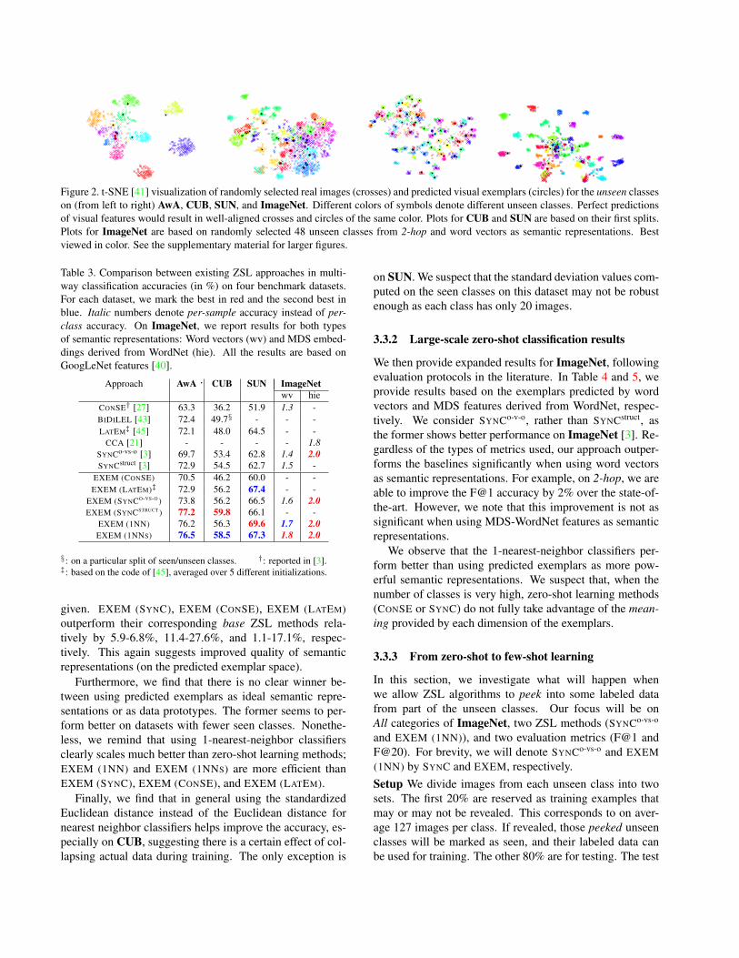
Figure 2. t-SNE [41] visualization of randomly selected real images (crosses) and predicted visual exemplars (circles) for the unseen classeson (from left to right) AwA, CUB, SUN, and ImageNet. Different colors of symbols denote different unseen classes. Perfect predictionsof visual features would result in well-aligned crosses and circles of the same color. Plots for CUB and SUN are based on their first splits.Plots for ImageNet are based on randomly selected 48 unseen classes from 2-hop and word vectors as semantic representations. Bestviewed in color. See the supplementary material for larger figures.

Table 3. Comparison between existing ZSL approaches in multi-way classification accuracies (in %) on four benchmark datasets.For each dataset, we mark the best in red and the second best inblue. Italic numbers denote per-sample accuracy instead of per-class accuracy. On ImageNet, we report results for both typesof semantic representations: Word vectors (wv) and MDS embed-dings derived from WordNet (hie). All the results are based onGoogLeNet features [40].

.Approach AwA CUB SUN ImageNetwv hie

CONSE† [27] 63.3 36.2 51.9 1.3 -BIDILEL [43] 72.4 49.7§ - - -LATEM‡ [45] 72.1 48.0 64.5 - -

CCA [21] - - - - 1.8SYNCo-vs-o [3] 69.7 53.4 62.8 1.4 2.0SYNCstruct [3] 72.9 54.5 62.7 1.5 -

EXEM (CONSE) 70.5 46.2 60.0 - -EXEM (LATEM)‡ 72.9 56.2 67.4 - -

EXEM (SYNCO-VS-O ) 73.8 56.2 66.5 1.6 2.0EXEM (SYNCSTRUCT ) 77.2 59.8 66.1 - -

EXEM (1NN) 76.2 56.3 69.6 1.7 2.0EXEM (1NNS) 76.5 58.5 67.3 1.8 2.0

§: on a particular split of seen/unseen classes. †: reported in [3].‡: based on the code of [45], averaged over 5 different initializations.

given. EXEM (SYNC), EXEM (CONSE), EXEM (LATEM)outperform their corresponding base ZSL methods rela-tively by 5.9-6.8%, 11.4-27.6%, and 1.1-17.1%, respec-tively. This again suggests improved quality of semanticrepresentations (on the predicted exemplar space).

Furthermore, we find that there is no clear winner be-tween using predicted exemplars as ideal semantic repre-sentations or as data prototypes. The former seems to per-form better on datasets with fewer seen classes. Nonethe-less, we remind that using 1-nearest-neighbor classifiersclearly scales much better than zero-shot learning methods;EXEM (1NN) and EXEM (1NNS) are more efficient thanEXEM (SYNC), EXEM (CONSE), and EXEM (LATEM).

Finally, we find that in general using the standardizedEuclidean distance instead of the Euclidean distance fornearest neighbor classifiers helps improve the accuracy, es-pecially on CUB, suggesting there is a certain effect of col-lapsing actual data during training. The only exception is

on SUN. We suspect that the standard deviation values com-puted on the seen classes on this dataset may not be robustenough as each class has only 20 images.

3.3.2 Large-scale zero-shot classification results

We then provide expanded results for ImageNet, followingevaluation protocols in the literature. In Table 4 and 5, weprovide results based on the exemplars predicted by wordvectors and MDS features derived from WordNet, respec-tively. We consider SYNCo-v-o, rather than SYNCstruct, asthe former shows better performance on ImageNet [3]. Re-gardless of the types of metrics used, our approach outper-forms the baselines significantly when using word vectorsas semantic representations. For example, on 2-hop, we areable to improve the F@1 accuracy by 2% over the state-of-the-art. However, we note that this improvement is not assignificant when using MDS-WordNet features as semanticrepresentations.

We observe that the 1-nearest-neighbor classifiers per-form better than using predicted exemplars as more pow-erful semantic representations. We suspect that, when thenumber of classes is very high, zero-shot learning methods(CONSE or SYNC) do not fully take advantage of the mean-ing provided by each dimension of the exemplars.

3.3.3 From zero-shot to few-shot learning

In this section, we investigate what will happen whenwe allow ZSL algorithms to peek into some labeled datafrom part of the unseen classes. Our focus will be onAll categories of ImageNet, two ZSL methods (SYNCo-vs-o

and EXEM (1NN)), and two evaluation metrics (F@1 andF@20). For brevity, we will denote SYNCo-vs-o and EXEM(1NN) by SYNC and EXEM, respectively.Setup We divide images from each unseen class into twosets. The first 20% are reserved as training examples thatmay or may not be revealed. This corresponds to on aver-age 127 images per class. If revealed, those peeked unseenclasses will be marked as seen, and their labeled data canbe used for training. The other 80% are for testing. The test

Table 4. Comparison between existing ZSL approaches on ImageNet using word vectors of the class names as semantic representations.For both metrics (in %), the higher the better. The best is in red. The numbers of unseen classes are listed in parentheses. †: reported in [3].

Test data Approach Flat Hit@K Hierarchical precision@KK= 1 2 5 10 20 2 5 10 20

CONSE† [27] 8.3 12.9 21.8 30.9 41.7 21.5 23.8 27.5 31.3SYNCo-vs-o [3] 10.5 16.7 28.6 40.1 52.0 25.1 27.7 30.3 32.1

2-hop (1,509) EXEM (SYNCO-VS-O ) 11.8 18.9 31.8 43.2 54.8 25.6 28.1 30.2 31.6EXEM (1NN) 11.7 18.3 30.9 42.7 54.8 25.9 28.5 31.2 33.3EXEM (1NNS) 12.5 19.5 32.3 43.7 55.2 26.9 29.1 31.1 32.0CONSE† [27] 2.6 4.1 7.3 11.1 16.4 6.7 21.4 23.8 26.3SYNCo-vs-o [3] 2.9 4.9 9.2 14.2 20.9 7.4 23.7 26.4 28.6

3-hop (7,678) EXEM (SYNCO-VS-O ) 3.4 5.6 10.3 15.7 22.8 7.5 24.7 27.3 29.5EXEM (1NN) 3.4 5.7 10.3 15.6 22.7 8.1 25.3 27.8 30.1EXEM (1NNS) 3.6 5.9 10.7 16.1 23.1 8.2 25.2 27.7 29.9CONSE† [27] 1.3 2.1 3.8 5.8 8.7 3.2 9.2 10.7 12.0SYNCo-vs-o [3] 1.4 2.4 4.5 7.1 10.9 3.1 9.0 10.9 12.5

All (20,345) EXEM (SYNCO-VS-O ) 1.6 2.7 5.0 7.8 11.8 3.2 9.3 11.0 12.5EXEM (1NN) 1.7 2.8 5.2 8.1 12.1 3.7 10.4 12.1 13.5EXEM (1NNS) 1.8 2.9 5.3 8.2 12.2 3.6 10.2 11.8 13.2

Table 5. Comparison between existing ZSL approaches on Im-ageNet (with 20,842 unseen classes) using MDS embeddingsderived from WordNet [21] as semantic representations. Thehigher, the better (in %). The best is in red.

Test data Approach Flat Hit@KK= 1 2 5 10 20

CCA [21] 1.8 3.0 5.2 7.3 9.7All SYNCo-vs-o [3] 2.0 3.4 6.0 8.8 12.5

(20,842) EXEM (SYNCO-VS-O ) 2.0 3.3 6.1 9.0 12.9EXEM (1NN) 2.0 3.4 6.3 9.2 13.1EXEM (1NNS) 2.0 3.4 6.2 9.2 13.2

Seen class index Unseen class index

Inst

ance

ind

ex 20 % for revealing

80 % for testing

: training data from seen classes

: additional training data from peeked unseen classes

: test data

: untouched data

Figure 3. Data split for zero-to-few-shot learning on ImageNet

set is always fixed such that we have to do few-shot learningfor peeked unseen classes and zero-shot learning on the restof the unseen classes. Fig. 3 summarizes this protocol.

We then vary the number of peeked unseen classes B.Also, for each of these numbers, we explore the followingsubset selection strategies (more details are in the supple-mentary material): (i) Uniform random: Randomly se-lected B unseen classes from the uniform distribution; (ii)Heavy-toward-seen random Randomly selectedB classesthat are semantically similar to seen classes according tothe WordNet hierarchy; (iii) Light-toward-seen randomRandomly selectedB classes that are semantically far awayfrom seen classes; (iv) K-means clustering for coverageClasses whose semantic representations are nearest to eachcluster’s center, where semantic embeddings of the unseenclasses are grouped by k-means clustering with k = B; (v)DPP for diversity Sequentially selected classes by a greedyalgorithm for fixed-sized determinantal point processes (k-DPPs) [16] with the RBF kernel computed on semantic rep-resentations.

Results For each of the ZSL methods (EXEM and SYNC),we first compare different subset selection methods whenthe number of peeked unseen classes is small (up to 2,000)in Fig. 4. We see that the performances of different sub-set selection methods are consistent across ZSL meth-ods. Moreover, heavy-toward-seen classes are preferred forstrict metrics (Flat Hit@1) but clustering is preferred forflexible metrics (Flat Hit@20). This suggests that, for astrict metric, it is better to pick the classes that are seman-tically similar to what we have seen. On the other hand, ifthe metric is flexible, we should focus on providing cover-age for all the classes so each of them has knowledge theycan transfer from.

Next, using the best performing heavy-toward-seen se-lection, we focus on comparing EXEM and SYNC withlarger numbers of peeked unseen classes in Fig. 5. Whenthe number of peeked unseen classes is small, EXEM out-performs SYNC. (In fact, EXEM outperforms SYNC for eachsubset selection method in Fig. 4.) However, we observethat SYNC will finally catch up and surpass EXEM. Thisis not surprising; as we observe more labeled data (due tothe increase in peeked unseen set size), the setting will be-come more similar to supervised learning (few-shot learn-ing), where linear classifiers used in SYNC should outper-form nearest center classifiers used by EXEM. Nonetheless,we note that EXEM is more computationally advantageousthan SYNC. In particular, when training on 1K classes ofImageNet with over 1M images, EXEM takes 3 mins whileSYNC 1 hour. We provide additional results under this sce-nario in the supplementary material.

3.3.4 Analysis

PCA or not? Table 6 investigates the effect of PCA. Ingeneral, EXEM (1NN) performs comparably with and with-out PCA. Moreover, decreasing PCA projected dimension dfrom 1024 to 500 does not hurt the performance. Clearly, a

0 500 1000 1500 20000.01

0.015

0.02

0.025

0.03

0.035

0.04

0.045

0.05

# peeked unseen classes

a

ccu

racy

EXEM: F@1

uniform

heavy−seen

clustering

light−seen

DPP

0 500 1000 1500 20000.01

0.015

0.02

0.025

0.03

0.035

0.04

0.045

0.05

# peeked unseen classes

accu

racy

SynC: F@1

uniform

heavy−seen

clustering

light−seen

DPP

0 500 1000 1500 20000.1

0.12

0.14

0.16

0.18

0.2

# peeked unseen classes

a

ccu

racy

EXEM: F@20

uniform

heavy−seen

clustering

light−seen

DPP

0 500 1000 1500 20000.1

0.12

0.14

0.16

0.18

0.2

# peeked unseen classes

accu

racy

SynC: F@20

uniform

heavy−seen

clustering

light−seen

DPP

Figure 4. Accuracy vs. the number of peeked unseen classes forEXEM (top) and SYNC (bottom) across different subset selectionmethods. Evaluation metrics are F@1 (left) and F@20 (right).

0 5000 10000 150000

0.02

0.04

0.06

0.08

0.1

0.12

0.14

0.16

# peeked unseen classes

a

ccura

cy

F@1

EXEM (heavy−seen)

SynC (heavy−seen)

0 5000 10000 150000.1

0.15

0.2

0.25

0.3

0.35

0.4

0.45

0.5

# peeked unseen classes

a

ccura

cy

F@20

EXEM (heavy−seen)

SynC (heavy−seen)

Figure 5. Accuracy vs. the number of peeked unseen classes forEXEM and SYNC for heavy-toward-seen class selection strategy.Evaluation metrics are F@1 (left) and F@20 (right).

Table 6. Accuracy of EXEM (1NN) on AwA, CUB, and SUN whenpredicted exemplars are from original visual features (No PCA)and PCA-projected features (PCA with d = 1024 and d = 500).

Dataset No PCA PCA PCAname d = 1024 d = 1024 d = 500AwA 77.8 76.2 76.2CUB 55.1 56.3 56.3SUN 69.2 69.6 69.6

Table 7. Comparison between EXEM (1NN) with support vector re-gressors (SVR) and with 2-layer multi-layer perceptron (MLP) forpredicting visual exemplars. Results on CUB are for the first split.Each number for MLP is an average over 3 random initialization.

Dataset How to predict No PCA PCA PCAname exemplars d = 1024 d = 1024 d = 500AwA SVR 77.8 76.2 76.2

MLP 76.1 ± 0.5 76.4 ± 0.1 75.5 ± 1.7CUB SVR 57.1 59.4 59.4

MLP 53.8 ± 0.3 54.2 ± 0.3 53.8 ± 0.5

smaller PCA dimension leads to faster computation due tofewer regressors to be trained. See additional results withother values for d in the supplementary material.Kernel regression vs. Multi-layer perceptron We com-pare two approaches for predicting visual exemplars:kernel-based support vector regressors (SVR) and 2-layermulti-layer perceptron (MLP) with ReLU nonlinearity.

MLP weights are `2 regularized, and we cross-validate theregularization constant. Additional details are in the sup-plementary material.

Table 7 shows that SVR performs more robustly thanMLP. One explanation is that MLP is prone to overfit-ting due to the small training set size (the number of seenclasses) as well as the model selection challenge imposedby ZSL scenarios. SVR also comes with other benefits; it ismore efficient and less susceptible to initialization.

4. Related Work

ZSL has been a popular research topic in both com-puter vision and machine learning. A general theme is tomake use of semantic representations such as attributes orword vectors to relate visual features of the seen and unseenclasses, as summarized in [1].

Our approach for predicting visual exemplars is inspiredby [12, 27]. They predict an image’s semantic embeddingfrom its visual features and compare to unseen classes’ se-mantic embeddings. As mentioned in Sect. 2.3, we perform“inverse prediction”: given an unseen class’s semantic rep-resentation, we predict where the exemplar visual featurevector for that class is in the semantic embedding space.

There has been a recent surge of interest in applying deeplearning models to generate images [22, 33, 46]. Most ofthese methods are based on probabilistic models (in order toincorporate the statistics of natural images). Unlike them,our prediction is to purely deterministically predict visualexemplars (features). Note that, generating features directlyis likely easier and more effective than generating realisticimages first and then extracting visual features from them.

5. Discussion

We have proposed a novel ZSL model that is simple butvery effective. Unlike previous approaches, our method di-rectly solves ZSL by predicting visual exemplars — clus-ter centers that characterize visual features of the unseenclasses of interest. This is made possible partly due to thewell separate cluster structure in the deep visual featurespace. We apply predicted exemplars to the task of zero-shot classification based on two views of these exemplars:ideal semantic representations and prototypical data points.Our approach achieves state-of-the-art performance on mul-tiple standard benchmark datasets. Finally, we also analyzeour approach and compliment our empirical studies with anextension of zero-shot to few-shot learning.

Acknowledgements This work is partially supportedby USC Graduate Fellowship, NSF IIS-1065243, 1451412,1513966/1632803, 1208500, CCF-1139148, a Google Re-search Award, an Alfred. P. Sloan Research Fellowshipand ARO# W911NF-12-1-0241 and W911NF-15-1-0484.

References[1] Z. Akata, F. Perronnin, Z. Harchaoui, and C. Schmid. Label-

embedding for attribute-based classification. In CVPR, 2013.1, 3, 8

[2] Z. Akata, S. Reed, D. Walter, H. Lee, and B. Schiele. Eval-uation of output embeddings for fine-grained image classifi-cation. In CVPR, 2015. 1, 3, 4

[3] S. Changpinyo, W.-L. Chao, B. Gong, and F. Sha. Synthe-sized classifiers for zero-shot learning. In CVPR, 2016. 1, 2,3, 4, 5, 6, 7

[4] W.-L. Chao, S. Changpinyo, B. Gong, and F. Sha. An empir-ical study and analysis of generalized zero-shot learning forobject recognition in the wild. In ECCV, 2016. 1, 3, 5

[5] C.-Y. Chen and K. Grauman. Inferring analogous attributes.In CVPR, 2014. 1

[6] T. Chilimbi, Y. Suzue, J. Apacible, and K. Kalyanaraman.Project Adam: Building an efficient and scalable deep learn-ing training system. In OSDI, 2014. 1

[7] K. Crammer and Y. Singer. On the algorithmic implemen-tation of multiclass kernel-based vector machines. JMLR,2:265–292, 2002. 4

[8] J. Deng, W. Dong, R. Socher, L.-J. Li, K. Li, and L. Fei-Fei. Imagenet: A large-scale hierarchical image database. InCVPR, 2009. 4

[9] K. Duan, D. Parikh, D. Crandall, and K. Grauman. Dis-covering localized attributes for fine-grained recognition. InCVPR, 2012. 1

[10] M. Elhoseiny, B. Saleh, and A. Elgammal. Write a classi-fier: Zero-shot learning using purely textual descriptions. InICCV, 2013. 1

[11] A. Farhadi, I. Endres, D. Hoiem, and D. Forsyth. Describingobjects by their attributes. In CVPR, 2009. 1, 3

[12] A. Frome, G. S. Corrado, J. Shlens, S. Bengio, J. Dean,M. Ranzato, and T. Mikolov. Devise: A deep visual-semanticembedding model. In NIPS, 2013. 1, 3, 4, 8

[13] D. Jayaraman and K. Grauman. Zero-shot recognition withunreliable attributes. In NIPS, 2014. 1, 3

[14] D. Jayaraman, F. Sha, and K. Grauman. Decorrelating se-mantic visual attributes by resisting the urge to share. InCVPR, 2014. 1

[15] N. Karessli, Z. Akata, A. Bulling, and B. Schiele. Gaze em-beddings for zero-shot image classification. In CVPR, 2017.1

[16] A. Kulesza and B. Taskar. k-dpps: Fixed-size determinantalpoint processes. In ICML, 2011. 7

[17] C. H. Lampert, H. Nickisch, and S. Harmeling. Learning todetect unseen object classes by between-class attribute trans-fer. In CVPR, 2009. 1, 3

[18] C. H. Lampert, H. Nickisch, and S. Harmeling. Attribute-based classification for zero-shot visual object categoriza-tion. TPAMI, 36(3):453–465, 2014. 4

[19] J. Lei Ba, K. Swersky, S. Fidler, and R. Salakhutdinov. Pre-dicting deep zero-shot convolutional neural networks usingtextual descriptions. In ICCV, 2015. 1

[20] Y. Long, L. Liu, L. Shao, F. Shen, G. Ding, and J. Han. Fromzero-shot learning to conventional supervised classification:Unseen visual data synthesis. In CVPR, 2017. 3

[21] Y. Lu. Unsupervised learning of neural network outputs:with application in zero-shot learning. In IJCAI, 2016. 1,3, 4, 5, 6, 7

[22] E. Mansimov, E. Parisotto, J. L. Ba, and R. Salakhutdinov.Generating images from captions with attention. In ICLR,2016. 8

[23] T. Mensink, E. Gavves, and C. G. Snoek. Costa: Co-occurrence statistics for zero-shot classification. In CVPR,2014. 3

[24] T. Mensink, J. Verbeek, F. Perronnin, and G. Csurka.Distance-based image classification: Generalizing to newclasses at near-zero cost. TPAMI, 35(11):2624–2637, 2013.3, 4

[25] T. Mikolov, K. Chen, G. S. Corrado, and J. Dean. Efficientestimation of word representations in vector space. In ICLRWorkshops, 2013. 4

[26] G. A. Miller. Wordnet: a lexical database for english. Com-munications of the ACM, 38(11):39–41, 1995. 1

[27] M. Norouzi, T. Mikolov, S. Bengio, Y. Singer, J. Shlens,A. Frome, G. S. Corrado, and J. Dean. Zero-shot learningby convex combination of semantic embeddings. In ICLR,2014. 1, 2, 3, 4, 5, 6, 7, 8

[28] M. Palatucci, D. Pomerleau, G. E. Hinton, and T. M.Mitchell. Zero-shot learning with semantic output codes. InNIPS, 2009. 1, 3

[29] D. Parikh and K. Grauman. Interactively building a discrim-inative vocabulary of nameable attributes. In CVPR, 2011.1

[30] G. Patterson, C. Xu, H. Su, and J. Hays. The sun attributedatabase: Beyond categories for deeper scene understanding.IJCV, 108(1-2):59–81, 2014. 4

[31] S.-A. Rebuffi, A. Kolesnikov, and C. H. Lampert. iCaRL:Incremental classifier and representation learning. In CVPR,2017. 4

[32] S. Reed, Z. Akata, H. Lee, and B. Schiele. Learning deeprepresentations of fine-grained visual descriptions. In CVPR,2016. 1

[33] S. Reed, Z. Akata, X. Yan, L. Logeswaran, H. Lee, andB. Schiele. Generative adversarial text to image synthesis.In ICML, 2016. 8

[34] M. Ristin, M. Guillaumin, J. Gall, and L. Van Gool. In-cremental learning of random forests for large-scale imageclassification. TPAMI, 38(3):490–503, 2016. 4

[35] B. Romera-Paredes and P. H. S. Torr. An embarrassinglysimple approach to zero-shot learning. In ICML, 2015. 1, 3

[36] O. Russakovsky, J. Deng, H. Su, J. Krause, S. Satheesh,S. Ma, Z. Huang, A. Karpathy, A. Khosla, M. Bernstein,A. C. Berg, and L. Fei-Fei. ImageNet Large Scale VisualRecognition Challenge. IJCV, 2015. 4

[37] R. Salakhutdinov, A. Torralba, and J. Tenenbaum. Learningto share visual appearance for multiclass object detection. InCVPR, 2011. 1

[38] B. Scholkopf, A. J. Smola, R. C. Williamson, and P. L.Bartlett. New support vector algorithms. Neural compu-tation, 12(5):1207–1245, 2000. 3

[39] R. Socher, M. Ganjoo, C. D. Manning, and A. Ng. Zero-shotlearning through cross-modal transfer. In NIPS, 2013. 1, 3

[40] C. Szegedy, W. Liu, Y. Jia, P. Sermanet, S. Reed,D. Anguelov, D. Erhan, V. Vanhoucke, and A. Rabinovich.Going deeper with convolutions. In CVPR, 2015. 4, 6

[41] L. Van der Maaten and G. Hinton. Visualizing data usingt-sne. JMLR, 9(2579-2605):85, 2008. 5, 6

[42] C. Wah, S. Branson, P. Welinder, P. Perona, and S. Belongie.The Caltech-UCSD Birds-200-2011 Dataset. Technical Re-port CNS-TR-2011-001, California Institute of Technology,2011. 4

[43] Q. Wang and K. Chen. Zero-shot visual recogni-tion via bidirectional latent embedding. arXiv preprintarXiv:1607.02104, 2016. 3, 4, 6

[44] Y. Xian, Z. Akata, and B. Schiele. Zero-shot learning – theGood, the Bad and the Ugly. In CVPR, 2017. 1, 4, 5

[45] Y. Xian, Z. Akata, G. Sharma, Q. Nguyen, M. Hein, andB. Schiele. Latent embeddings for zero-shot classification.In CVPR, 2016. 1, 4, 5, 6

[46] X. Yan, J. Yang, K. Sohn, and H. Lee. Attribute2image: Con-ditional image generation from visual attributes. In ECCV,2016. 8

[47] F. X. Yu, L. Cao, R. S. Feris, J. R. Smith, and S.-F. Chang.Designing category-level attributes for discriminative visualrecognition. In CVPR, 2013. 1, 3

[48] L. Zhang, T. Xiang, and S. Gong. Learning a deep embed-ding model for zero-shot learning. In CVPR, 2017. 4, 5

[49] Z. Zhang and V. Saligrama. Zero-shot learning via semanticsimilarity embedding. In ICCV, 2015. 1, 3, 5

[50] Z. Zhang and V. Saligrama. Zero-shot learning via joint la-tent similarity embedding. In CVPR, 2016. 1, 3

[51] X. Zhu, D. Anguelov, and D. Ramanan. Capturing long-taildistributions of object subcategories. In CVPR, 2014. 1