predicting time-to-event outcomes based on high ... events... · high-dimensional multivariate...
TRANSCRIPT

Predicting time-to-event outcomes based on
high-dimensional multivariate longitudinal information
EFSPI: Brussels, November 7, 2013
Geert Verbeke
Interuniversity Institute for Biostatistics and statistical Bioinformatics
http://perswww.kuleuven.be/geert verbeke
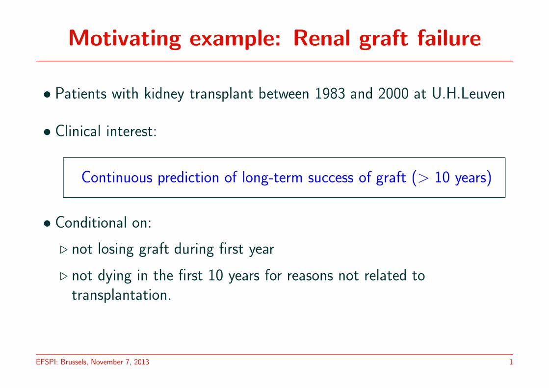
Motivating example: Renal graft failure
• Patients with kidney transplant between 1983 and 2000 at U.H.Leuven
• Clinical interest:
Continuous prediction of long-term success of graft (> 10 years)
• Conditional on:
. not losing graft during first year
. not dying in the first 10 years for reasons not related totransplantation.
EFSPI: Brussels, November 7, 2013 1
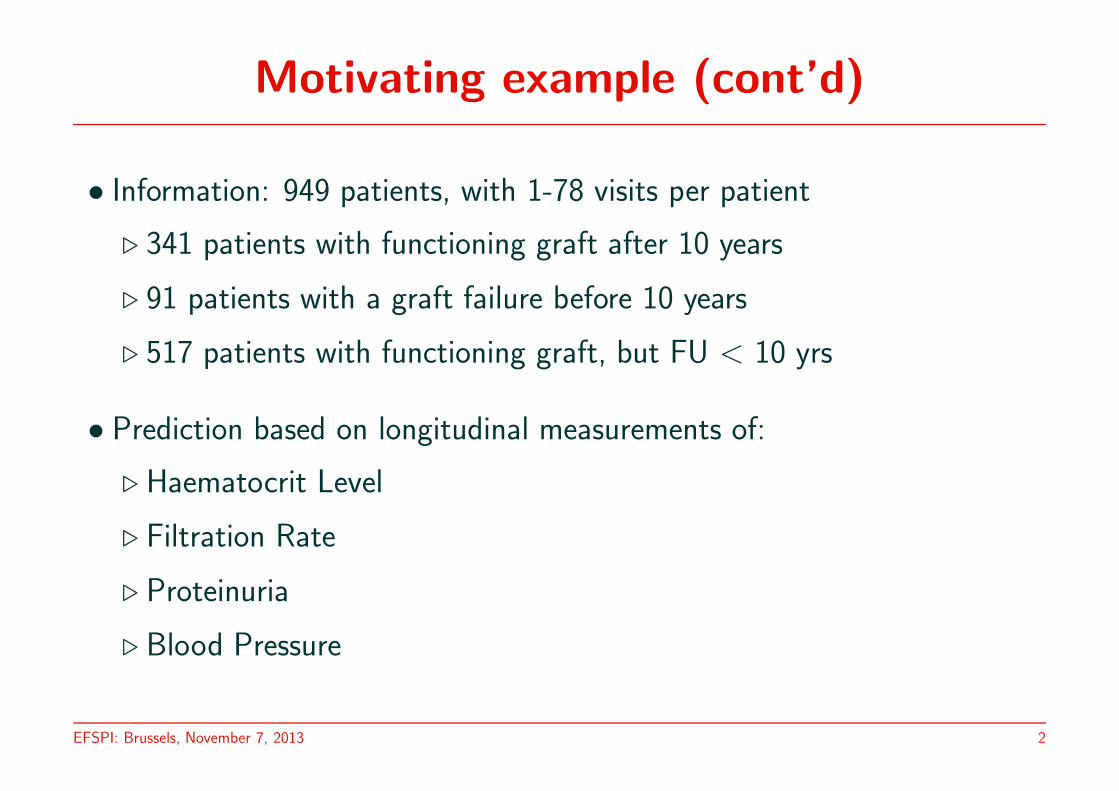
Motivating example (cont’d)
• Information: 949 patients, with 1-78 visits per patient
. 341 patients with functioning graft after 10 years
. 91 patients with a graft failure before 10 years
. 517 patients with functioning graft, but FU < 10 yrs
• Prediction based on longitudinal measurements of:
. Haematocrit Level
. Filtration Rate
. Proteinuria
. Blood Pressure
EFSPI: Brussels, November 7, 2013 2
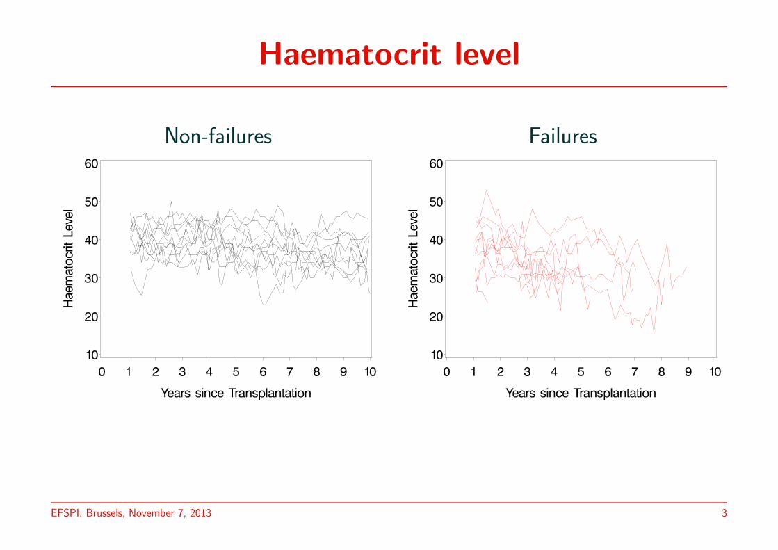
Haematocrit level
Non-failures Failures
EFSPI: Brussels, November 7, 2013 3
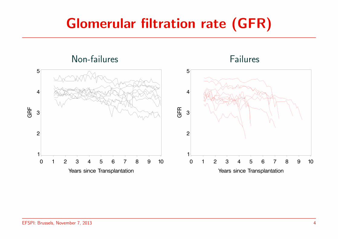
Glomerular filtration rate (GFR)
Non-failures Failures
EFSPI: Brussels, November 7, 2013 4
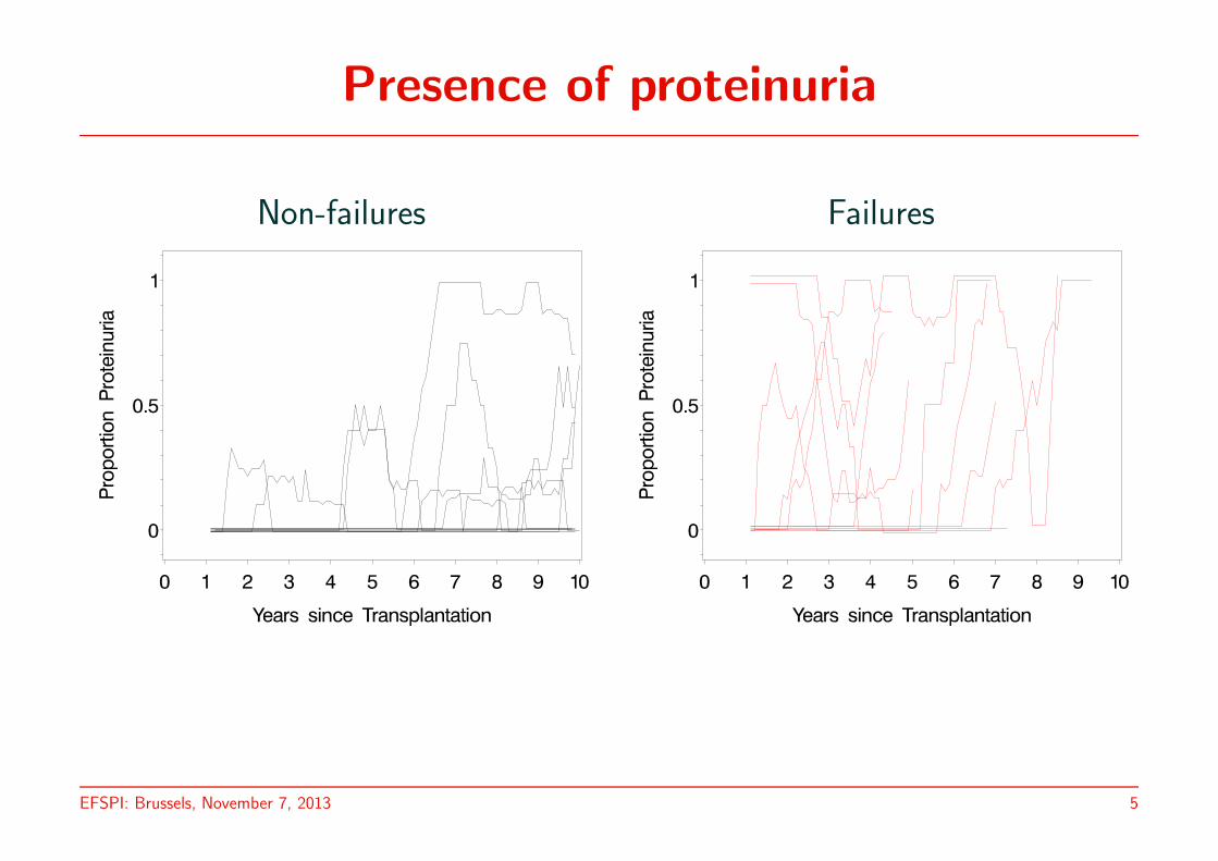
Presence of proteinuria
Non-failures Failures
EFSPI: Brussels, November 7, 2013 5
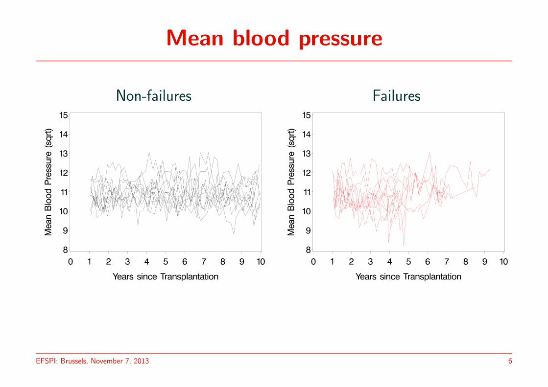
Mean blood pressure
Non-failures Failures
EFSPI: Brussels, November 7, 2013 6
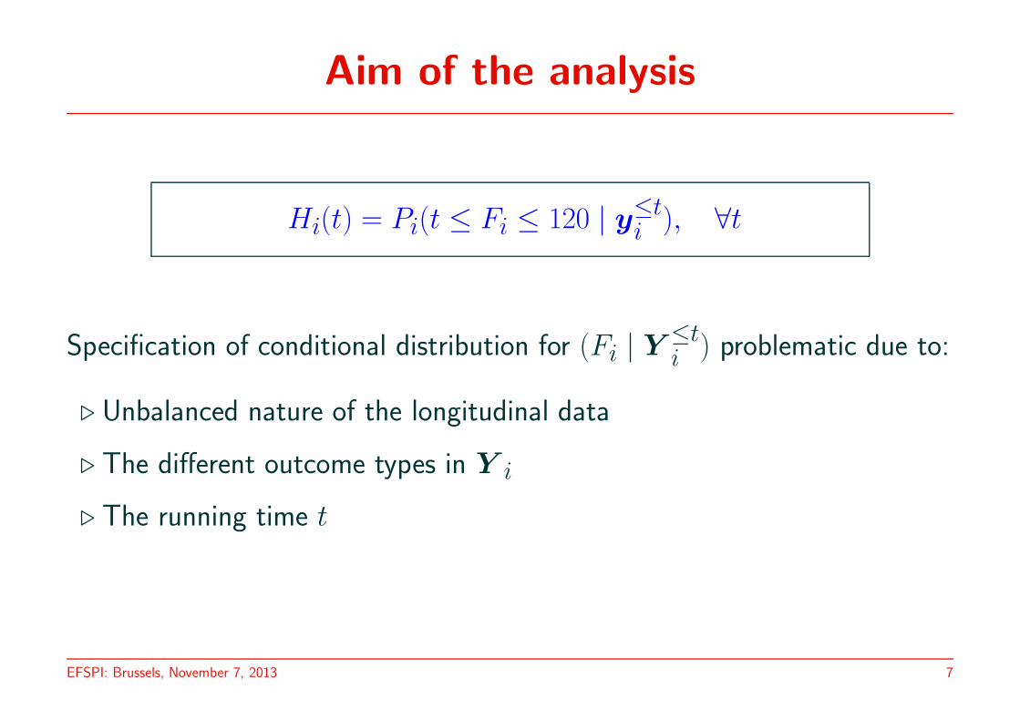
Aim of the analysis
Hi(t) = Pi(t ≤ Fi ≤ 120 | y≤ti ), ∀t
Specification of conditional distribution for (Fi | Y ≤ti ) problematic due to:
. Unbalanced nature of the longitudinal data
. The different outcome types in Y i
. The running time t
EFSPI: Brussels, November 7, 2013 7

A pattern-mixture approach
f (Fi,Y i) = f (Y i|Fi)f (Fi)
⇓f (Fi,Y
≤ti ) = f (Y ≤t
i |Fi)f (Fi)
⇓ + Bayes rule
Hi(t) = Pi(t ≤ Fi ≤ 120 | y≤ti )
= fi(y≤t
i| t ≤ Fi ≤ 120)P (Fi ≤ 120|Fi ≥ t)
fi(y≤t
i| t ≤ Fi ≤ 120)P (Fi ≤ 120|Fi ≥ t) + fi(y
≤t
i| Fi > 120)P (Fi > 120|Fi ≥ t)
EFSPI: Brussels, November 7, 2013 8
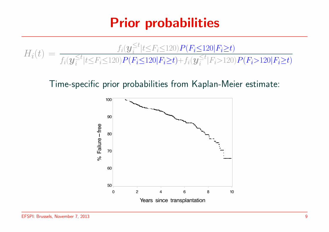
Prior probabilities
Hi(t) =fi(y
≤t
i|t≤Fi≤120)P (Fi≤120|Fi≥t)
fi(y≤t
i|t≤Fi≤120)P (Fi≤120|Fi≥t)+fi(y
≤t
i|Fi>120)P (Fi>120|Fi≥t)
Time-specific prior probabilities from Kaplan-Meier estimate:
EFSPI: Brussels, November 7, 2013 9
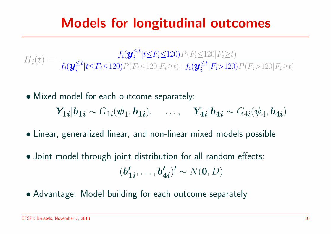
Models for longitudinal outcomes
Hi(t) =fi(y
≤t
i|t≤Fi≤120)P (Fi≤120|Fi≥t)
fi(y≤t
i|t≤Fi≤120)P (Fi≤120|Fi≥t)+fi(y
≤t
i|Fi>120)P (Fi>120|Fi≥t)
• Mixed model for each outcome separately:
Y1i|b1i ∼ G1i(ψ1, b1i), . . . , Y4i|b4i ∼ G4i(ψ4, b4i)
• Linear, generalized linear, and non-linear mixed models possible
• Joint model through joint distribution for all random effects:
(b′1i, . . . , b
′
4i)′ ∼ N (0, D)
• Advantage: Model building for each outcome separately
EFSPI: Brussels, November 7, 2013 10
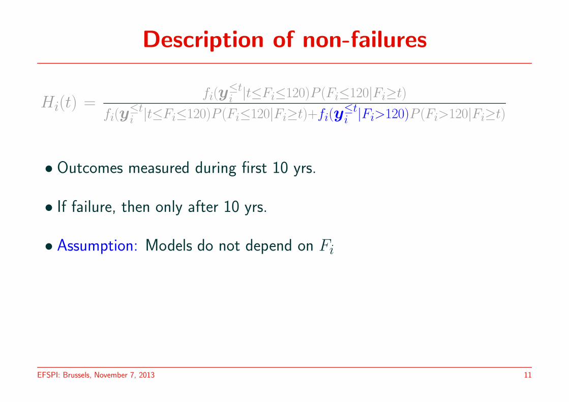
Description of non-failures
Hi(t) =fi(y
≤t
i|t≤Fi≤120)P (Fi≤120|Fi≥t)
fi(y≤t
i|t≤Fi≤120)P (Fi≤120|Fi≥t)+fi(y
≤t
i|Fi>120)P (Fi>120|Fi≥t)
• Outcomes measured during first 10 yrs.
• If failure, then only after 10 yrs.
• Assumption: Models do not depend on Fi
EFSPI: Brussels, November 7, 2013 11
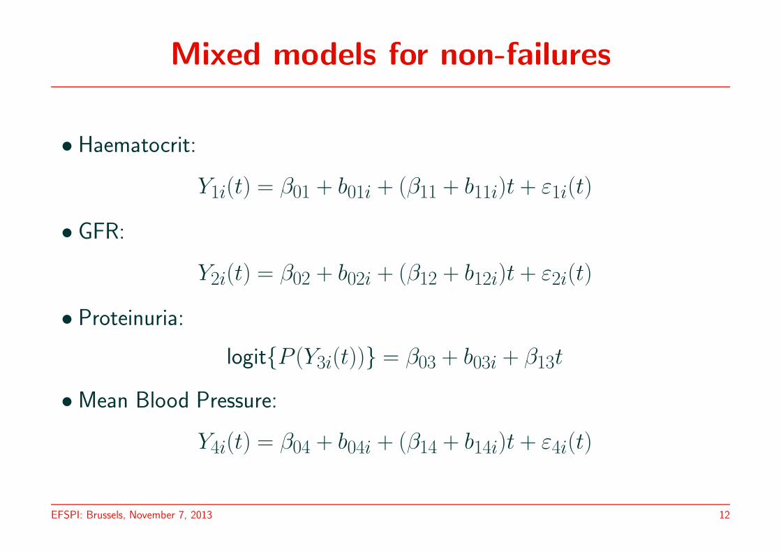
Mixed models for non-failures
• Haematocrit:
Y1i(t) = β01 + b01i + (β11 + b11i)t + ε1i(t)
• GFR:
Y2i(t) = β02 + b02i + (β12 + b12i)t + ε2i(t)
• Proteinuria:
logit{P (Y3i(t))} = β03 + b03i + β13t
• Mean Blood Pressure:
Y4i(t) = β04 + b04i + (β14 + b14i)t + ε4i(t)
EFSPI: Brussels, November 7, 2013 12
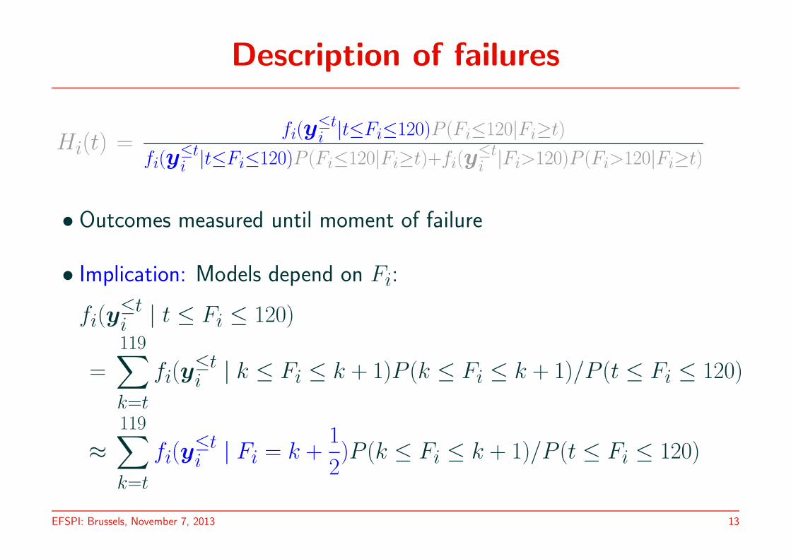
Description of failures
Hi(t) =fi(y
≤t
i|t≤Fi≤120)P (Fi≤120|Fi≥t)
fi(y≤t
i|t≤Fi≤120)P (Fi≤120|Fi≥t)+fi(y
≤t
i|Fi>120)P (Fi>120|Fi≥t)
• Outcomes measured until moment of failure
• Implication: Models depend on Fi:
fi(y≤ti | t ≤ Fi ≤ 120)
=
119∑
k=t
fi(y≤ti | k ≤ Fi ≤ k + 1)P (k ≤ Fi ≤ k + 1)/P (t ≤ Fi ≤ 120)
≈119∑
k=t
fi(y≤ti | Fi = k +
1
2)P (k ≤ Fi ≤ k + 1)/P (t ≤ Fi ≤ 120)
EFSPI: Brussels, November 7, 2013 13
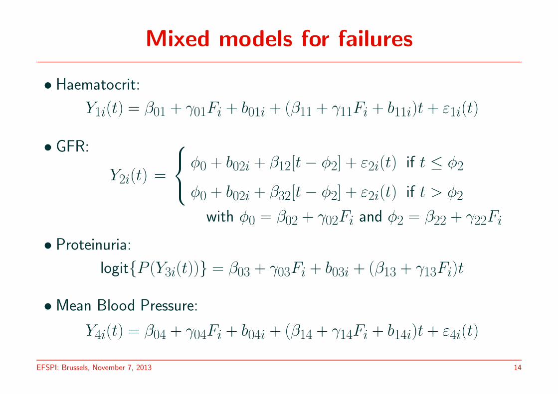
Mixed models for failures
• Haematocrit:
Y1i(t) = β01 + γ01Fi + b01i + (β11 + γ11Fi + b11i)t + ε1i(t)
• GFR:
Y2i(t) =
φ0 + b02i + β12[t − φ2] + ε2i(t) if t ≤ φ2
φ0 + b02i + β32[t − φ2] + ε2i(t) if t > φ2
with φ0 = β02 + γ02Fi and φ2 = β22 + γ22Fi
• Proteinuria:
logit{P (Y3i(t))} = β03 + γ03Fi + b03i + (β13 + γ13Fi)t
• Mean Blood Pressure:
Y4i(t) = β04 + γ04Fi + b04i + (β14 + γ14Fi + b14i)t + ε4i(t)
EFSPI: Brussels, November 7, 2013 14

Mixed models: Summary
Non-Failures Failures
Haematocrit: LMM (2) LMM (2)
GFR: LMM (2) NLMM (1)
Proteinuria: GLMM (1) GLMM (1)
Mean Blood Pressure: LMM (2) LMM (2)
⇒ 2 mixed models with many random effects (7 & 6)
⇒ computational difficulties
EFSPI: Brussels, November 7, 2013 15
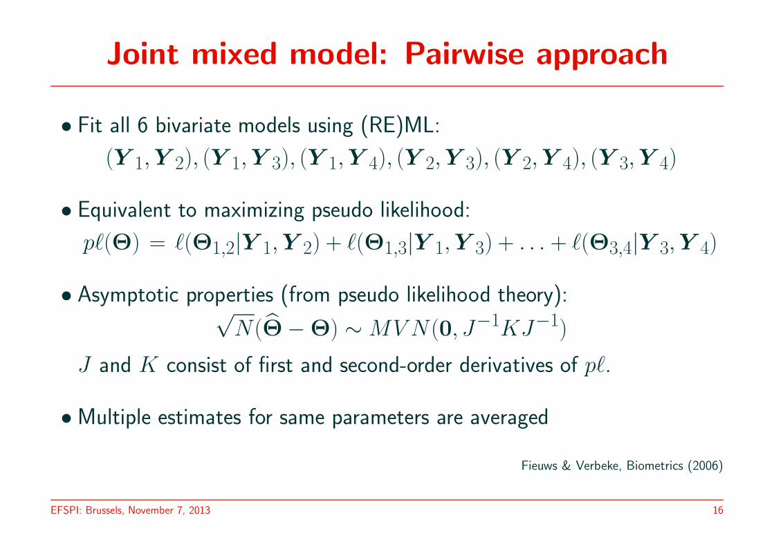
Joint mixed model: Pairwise approach
• Fit all 6 bivariate models using (RE)ML:
(Y 1,Y 2), (Y 1,Y 3), (Y 1,Y 4), (Y 2,Y 3), (Y 2,Y 4), (Y 3,Y 4)
• Equivalent to maximizing pseudo likelihood:
p`(Θ) = `(Θ1,2|Y 1,Y 2) + `(Θ1,3|Y 1,Y 3) + . . . + `(Θ3,4|Y 3,Y 4)
• Asymptotic properties (from pseudo likelihood theory):√N(Θ̂ − Θ) ∼ MV N (0, J−1KJ−1)
J and K consist of first and second-order derivatives of p`.
• Multiple estimates for same parameters are averaged
Fieuws & Verbeke, Biometrics (2006)
EFSPI: Brussels, November 7, 2013 16
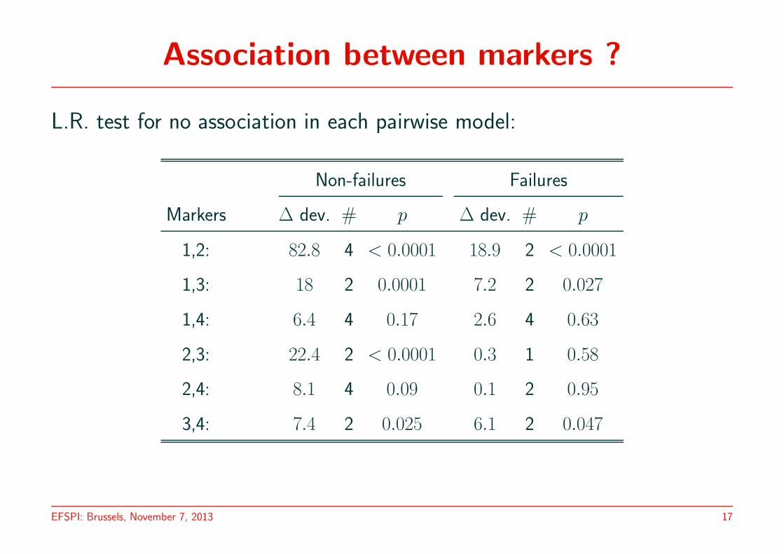
Association between markers ?
L.R. test for no association in each pairwise model:
Non-failures Failures
Markers ∆ dev. # p ∆ dev. # p
1,2: 82.8 4 < 0.0001 18.9 2 < 0.0001
1,3: 18 2 0.0001 7.2 2 0.027
1,4: 6.4 4 0.17 2.6 4 0.63
2,3: 22.4 2 < 0.0001 0.3 1 0.58
2,4: 8.1 4 0.09 0.1 2 0.95
3,4: 7.4 2 0.025 6.1 2 0.047
EFSPI: Brussels, November 7, 2013 17
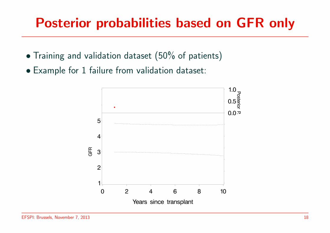
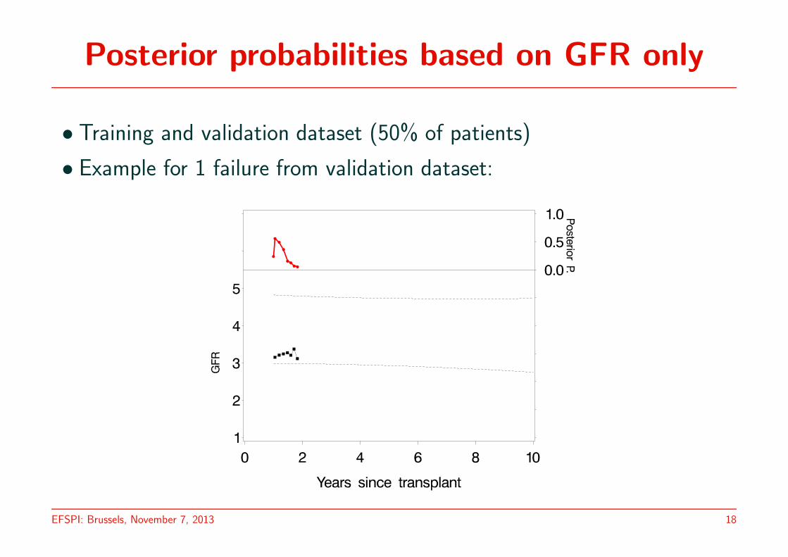
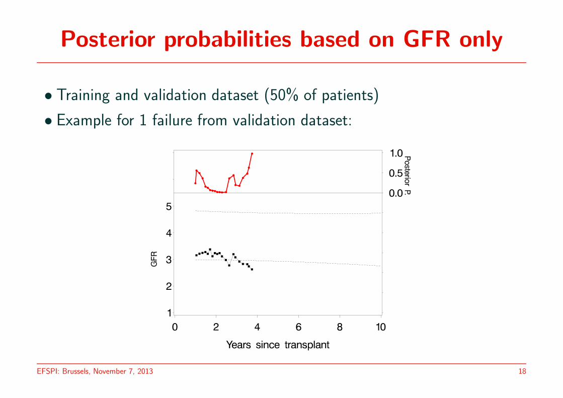
Posterior probabilities based on GFR only
• Training and validation dataset (50% of patients)
• Example for 1 failure from validation dataset:
EFSPI: Brussels, November 7, 2013 18

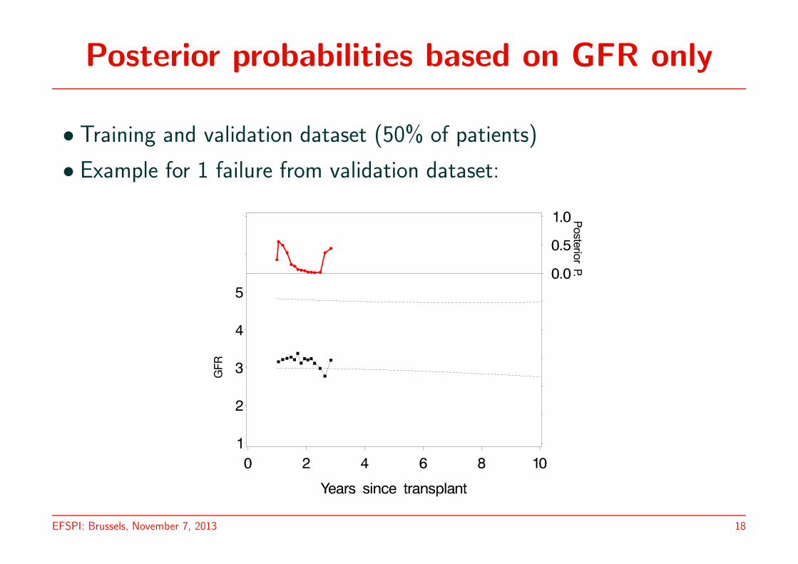
Posterior probabilities based on GFR only
• Training and validation dataset (50% of patients)
• Example for 1 failure from validation dataset:
EFSPI: Brussels, November 7, 2013 18

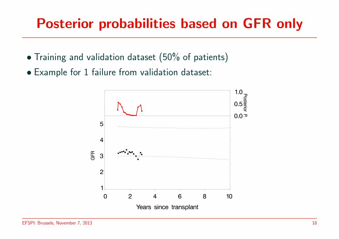
Posterior probabilities based on GFR only
• Training and validation dataset (50% of patients)
• Example for 1 failure from validation dataset:
EFSPI: Brussels, November 7, 2013 18

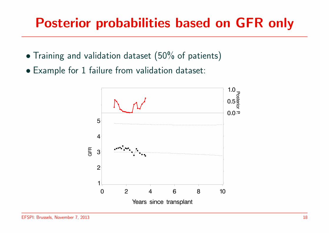
Posterior probabilities based on GFR only
• Training and validation dataset (50% of patients)
• Example for 1 failure from validation dataset:
EFSPI: Brussels, November 7, 2013 18

Posterior probabilities based on GFR only
• Training and validation dataset (50% of patients)
• Example for 1 failure from validation dataset:
EFSPI: Brussels, November 7, 2013 18

Posterior probabilities based on GFR only
• Training and validation dataset (50% of patients)
• Example for 1 failure from validation dataset:
EFSPI: Brussels, November 7, 2013 18

Posterior probabilities based on GFR only
• Training and validation dataset (50% of patients)
• Example for 1 failure from validation dataset:
EFSPI: Brussels, November 7, 2013 18
Posterior probabilities based on GFR only
• Training and validation dataset (50% of patients)
• Example for 1 failure from validation dataset:
EFSPI: Brussels, November 7, 2013 18

Posterior probabilities based on GFR only
• Training and validation dataset (50% of patients)
• Example for 1 failure from validation dataset:
EFSPI: Brussels, November 7, 2013 18

Posterior probabilities based on GFR only
• Training and validation dataset (50% of patients)
• Example for 1 failure from validation dataset:
EFSPI: Brussels, November 7, 2013 18

Posterior probabilities based on GFR only
• Training and validation dataset (50% of patients)
• Example for 1 failure from validation dataset:
EFSPI: Brussels, November 7, 2013 18

Posterior probabilities based on GFR only
• Training and validation dataset (50% of patients)
• Example for 1 failure from validation dataset:
EFSPI: Brussels, November 7, 2013 18

Posterior probabilities based on GFR only
• Training and validation dataset (50% of patients)
• Example for 1 failure from validation dataset:
EFSPI: Brussels, November 7, 2013 18

Posterior probabilities based on GFR only
• Training and validation dataset (50% of patients)
• Example for 1 failure from validation dataset:
EFSPI: Brussels, November 7, 2013 18
Posterior probabilities based on GFR only
• Training and validation dataset (50% of patients)
• Example for 1 failure from validation dataset:
EFSPI: Brussels, November 7, 2013 18
Posterior probabilities based on GFR only
• Training and validation dataset (50% of patients)
• Example for 1 failure from validation dataset:
EFSPI: Brussels, November 7, 2013 18

Posterior probabilities based on GFR only
• Training and validation dataset (50% of patients)
• Example for 1 failure from validation dataset:
EFSPI: Brussels, November 7, 2013 18

Posterior probabilities based on GFR only
• Training and validation dataset (50% of patients)
• Example for 1 failure from validation dataset:
EFSPI: Brussels, November 7, 2013 18

Posterior probabilities based on GFR only
• Training and validation dataset (50% of patients)
• Example for 1 failure from validation dataset:
EFSPI: Brussels, November 7, 2013 18
Posterior probabilities based on GFR only
• Training and validation dataset (50% of patients)
• Example for 1 failure from validation dataset:
EFSPI: Brussels, November 7, 2013 18
Posterior probabilities based on GFR only
• Training and validation dataset (50% of patients)
• Example for 1 failure from validation dataset:
EFSPI: Brussels, November 7, 2013 18
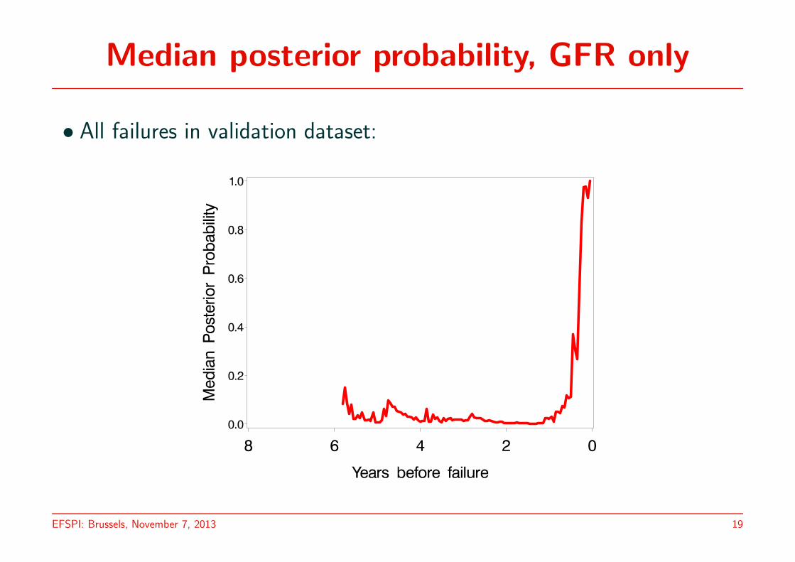
Median posterior probability, GFR only
• All failures in validation dataset:
EFSPI: Brussels, November 7, 2013 19

Discriminant analysis using 4 markers
Strategies:
• Decision based on highest posterior probability
• Joint model assuming uncorrelated markers
• Joint model allowing markers to be correlated
EFSPI: Brussels, November 7, 2013 20
Median posterior probability: Failures
• 46 patients in validation set who fail
• Median posterior probabilities to fail within the remaining period
• As a function of time: years before failure
EFSPI: Brussels, November 7, 2013 21
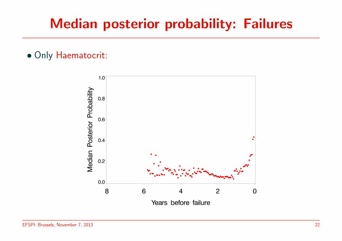
Median posterior probability: Failures
• Only Haematocrit:
EFSPI: Brussels, November 7, 2013 22
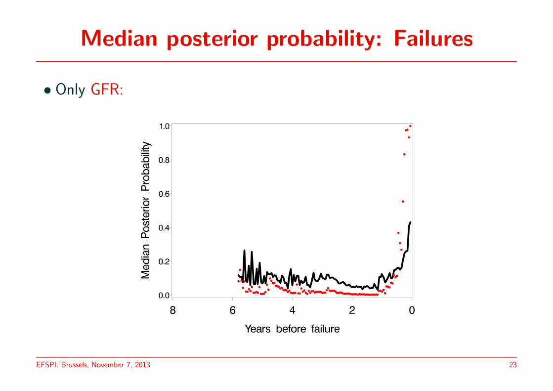
Median posterior probability: Failures
• Only GFR:
EFSPI: Brussels, November 7, 2013 23

Median posterior probability: Failures
• Only Proteinuria:
EFSPI: Brussels, November 7, 2013 24

Median posterior probability: Failures
• Only Mean Blood Pressure:
EFSPI: Brussels, November 7, 2013 25
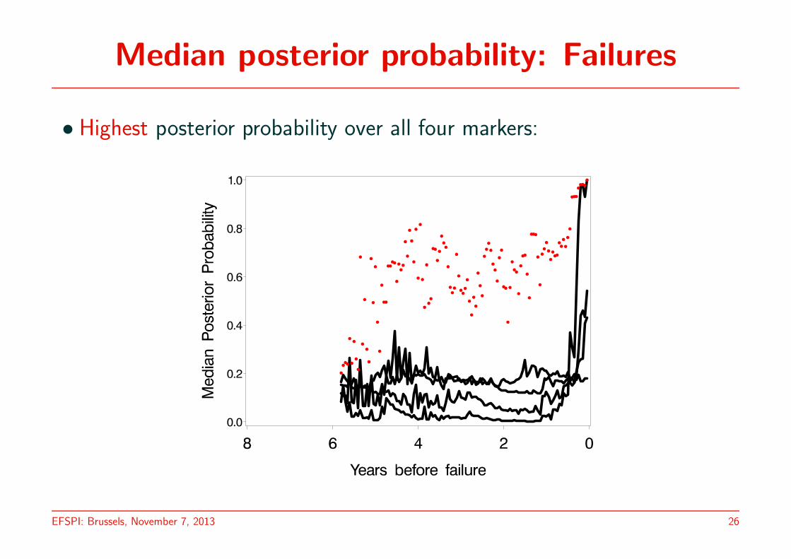
Median posterior probability: Failures
• Highest posterior probability over all four markers:
EFSPI: Brussels, November 7, 2013 26
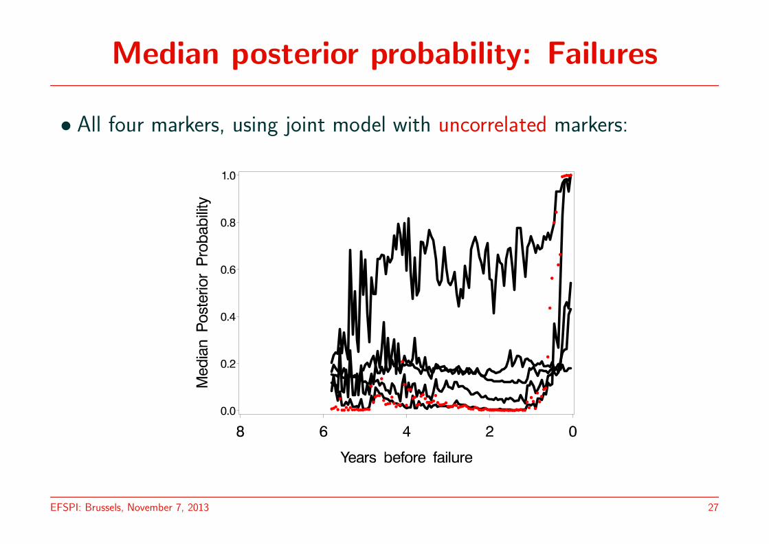
Median posterior probability: Failures
• All four markers, using joint model with uncorrelated markers:
EFSPI: Brussels, November 7, 2013 27
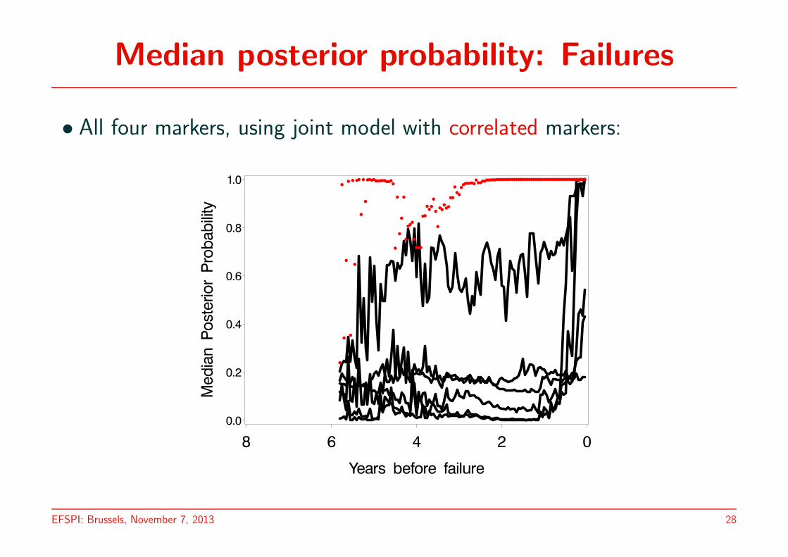
Median posterior probability: Failures
• All four markers, using joint model with correlated markers:
EFSPI: Brussels, November 7, 2013 28

Median posterior probability: Non-failures
• 171 patients in validation set who do not fail
• Median posterior probabilities to fail within the remaining period
• As a function of time: years since transplantation
EFSPI: Brussels, November 7, 2013 29

Median posterior probability: Non-failures
• Only Haematocrit:
EFSPI: Brussels, November 7, 2013 30
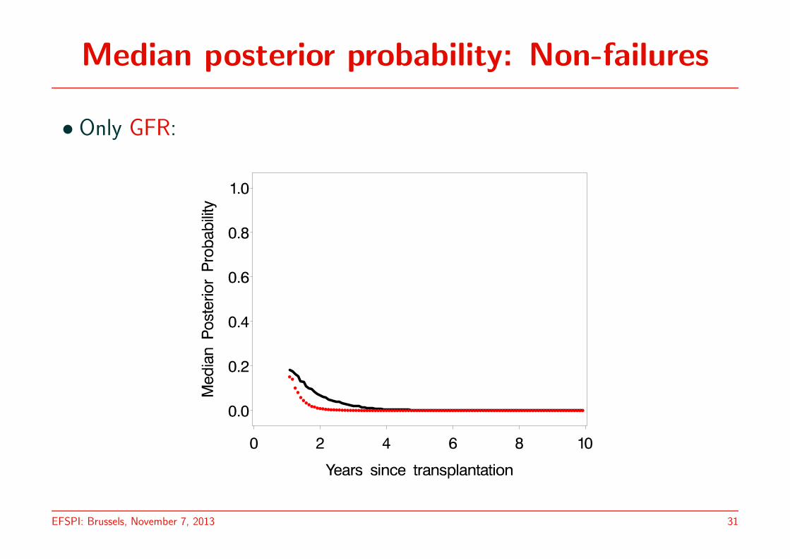
Median posterior probability: Non-failures
• Only GFR:
EFSPI: Brussels, November 7, 2013 31
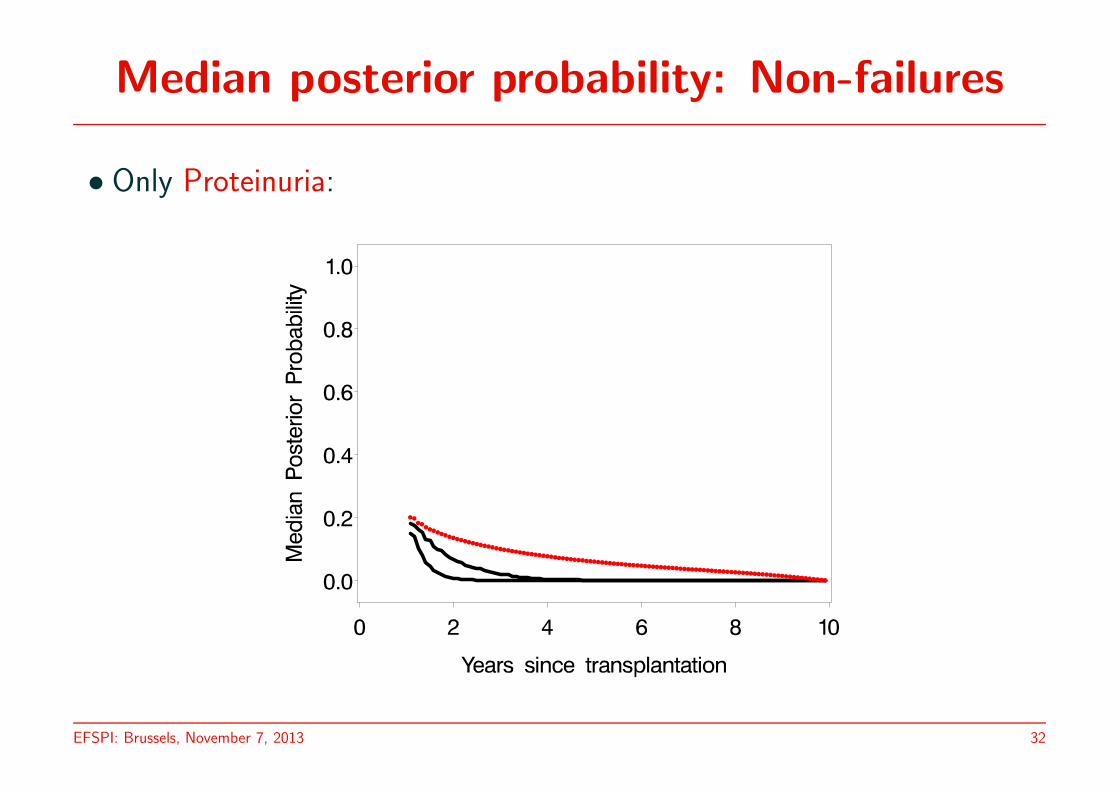
Median posterior probability: Non-failures
• Only Proteinuria:
EFSPI: Brussels, November 7, 2013 32
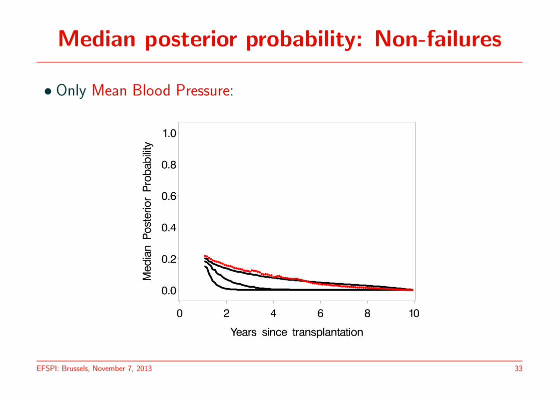
Median posterior probability: Non-failures
• Only Mean Blood Pressure:
EFSPI: Brussels, November 7, 2013 33

Median posterior probability: Non-failures
• Highest posterior probability over all four markers:
EFSPI: Brussels, November 7, 2013 34
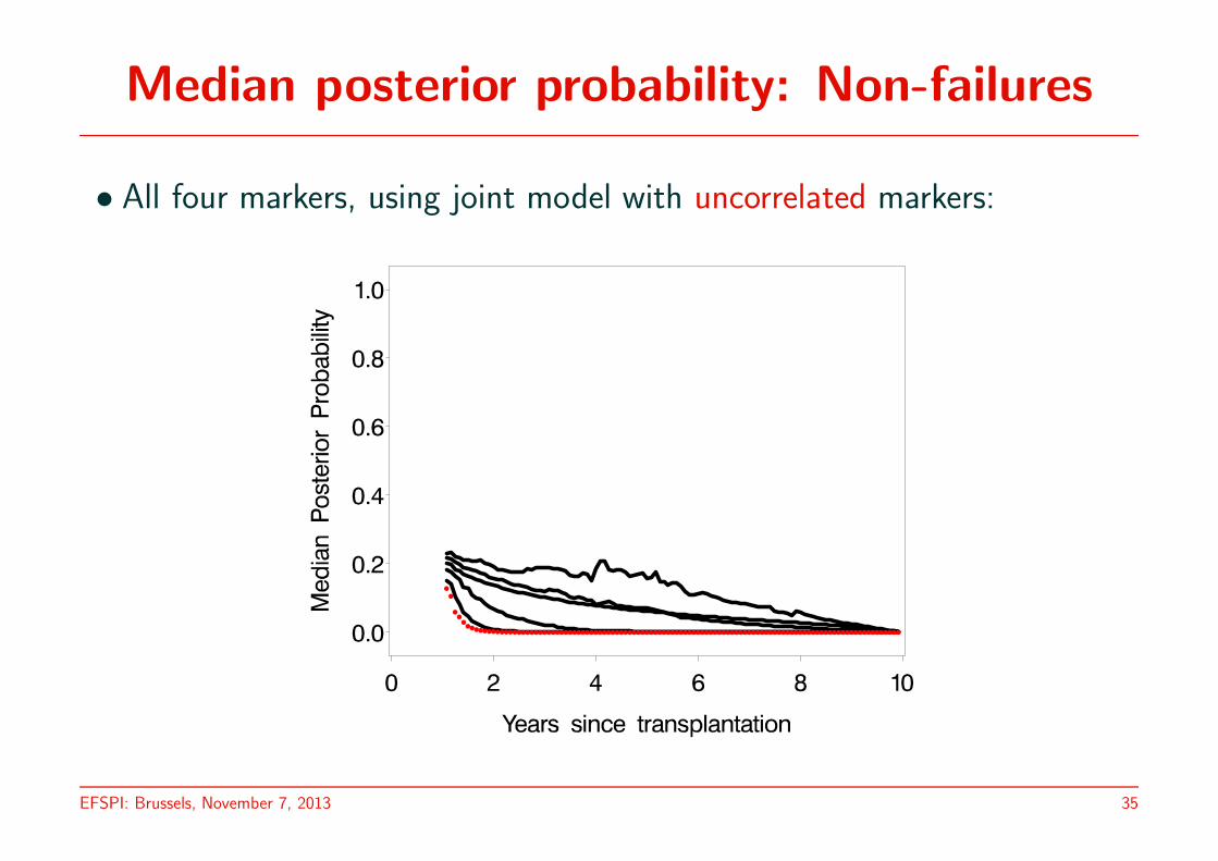
Median posterior probability: Non-failures
• All four markers, using joint model with uncorrelated markers:
EFSPI: Brussels, November 7, 2013 35
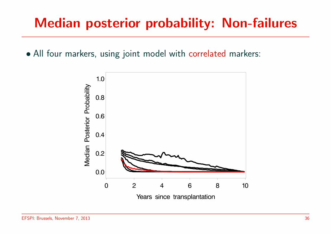
Median posterior probability: Non-failures
• All four markers, using joint model with correlated markers:
EFSPI: Brussels, November 7, 2013 36
Conclusions
• Discriminant analysis based on many outcomes, measured longitudinally,in an unbalanced design, is technically possible
• Allowing the longitudinal markers to be correlated considerably improvespredictions
• A pattern-mixture approach allows for continuous updating of posteriorprobabilities
• Various mixed models can be combined and fitted using pairwise fittingapproach
EFSPI: Brussels, November 7, 2013 37

The End !
EFSPI: Brussels, November 7, 2013 38