Predicting The Next App That You Are Going To Use

Ricardo Baeza-YatesYahoo Labs

Barcelona, Spainrbaeza@acm.org

Di Jiang∗

CS and Eng. Dept.HKUST, Hong Kong, China

dijiang@cse.ust.hkFabrizio Silvestri

Yahoo LabsBarcelona, Spain

silvestr@yahoo-inc.com

Beverly HarrisonYahoo Labs

Sunnyvale, USbeverlyh@yahoo-inc.com

ABSTRACTGiven the large number of installed apps and the limitedscreen size of mobile devices, it is often tedious for users tosearch for the app they want to use. Although some mo-bile OSs provide categorization schemes that enhance thevisibility of useful apps among those installed, the emergingcategory of homescreen apps aims to take one step further byautomatically organizing the installed apps in a more intel-ligent and personalized way. In this paper, we study how toimprove homescreen apps’ usage experience through a pre-diction mechanism that allows to show to users which appshe is going to use in the immediate future. The predictiontechnique is based on a set of features representing the real-time spatiotemporal contexts sensed by the homescreen app.We model the prediction of the next app as a classificationproblem and propose an effective personalized method tosolve it that takes full advantage of human-engineered fea-tures and automatically derived features. Furthermore, westudy how to solve the two naturally associated cold-startproblems: app cold-start and user cold-start. We conductlarge-scale experiments on log data obtained from YahooAviate, showing that our approach can accurately predictthe next app that a person is going to use.

Categories and Subject DescriptorsJ.0 [Computer Applications]: GENERAL.

General TermsDesign, Experimentation, Performance.

KeywordsAviate, Prediction, Mobile App, Machine Learning.

∗This work was done while the author was an intern at Ya-hoo Labs, Barcelona, Spain

Permission to make digital or hard copies of all or part of this work for personal orclassroom use is granted without fee provided that copies are not made or distributedfor profit or commercial advantage and that copies bear this notice and the full cita-tion on the first page. Copyrights for components of this work owned by others thanACM must be honored. Abstracting with credit is permitted. To copy otherwise, or re-publish, to post on servers or to redistribute to lists, requires prior specific permissionand/or a fee. Request permissions from permissions@acm.org.WSDM’15, February 2–6, 2015, Shanghai, China.Copyright 2015 ACM 978-1-4503-3317-7/15/02 ...$15.00.http://dx.doi.org/10.1145/2684822.2685302.

1. INTRODUCTIONMobile devices (smartphones and tables) are ubiquitous

in today’s lives. This high popularity also corresponds to ahuge growth in the availability and usage of mobile applica-tions (commonly referred to as apps). Mobile applicationsare very easy to install and this usually correspond to havingmobile phones with a very large number of apps installed.An empirical study conducted by Yahoo Aviate team showsthat on average there are 96 apps installed on each mobiledevice. This large number of apps installed calls for the de-sign of new paradigms aimed to manage the installed apps.In particular, one of the major issues associated with thehigh number of apps installed on a smartphone is that oftheir visibility. When a user needs a particular app it is notalways available immediately and the search through thelarge number of installed apps might take lots of time. Thisis the reason why homescreen apps are becoming more andmore popular. Homescreen apps act as an intelligent layerbetween the underlying mobile operating system and theuser interface. They manage the installed apps in a highlypersonalized manner rather than simply relying on manual(or trivial) categorization schemes.

The basic building block that we consider at the heartof an effective personalized management of apps is a per-sonalized app prediction mechanism. In other words, themost important feature of our homescreen app is that of an-ticipating the user needs even before the user would clickon the relative icon on his/her mobile phone. Ideally, oncethe predictor has made its guess the homescreen app shouldshow the application already opened as the user picks upthe phone and unlocks it. Even if this scenario might soundfuturistic, we show here that to predict which app a user isgoing to open, is actually feasible. Our solution leveragesthe sequence of real-time spatiotemporal contexts that arecontinuously sensed by the homescreen app (in this case, theYahoo Aviate application).

App Prediction Problem is formally defined as follows:Given a list of installed apps au1, au2, ..., aun by a user

u on his/her phone and the user’s spatiotemporal context C,the problem of app usage prediction is to find an app aui thathas the largest probability of being used under C. Specifically,we aim to solve the problem:

maxaui

P (aui|C, u), ∀i, 1 ≤ i ≤ n;

(a)

(b)

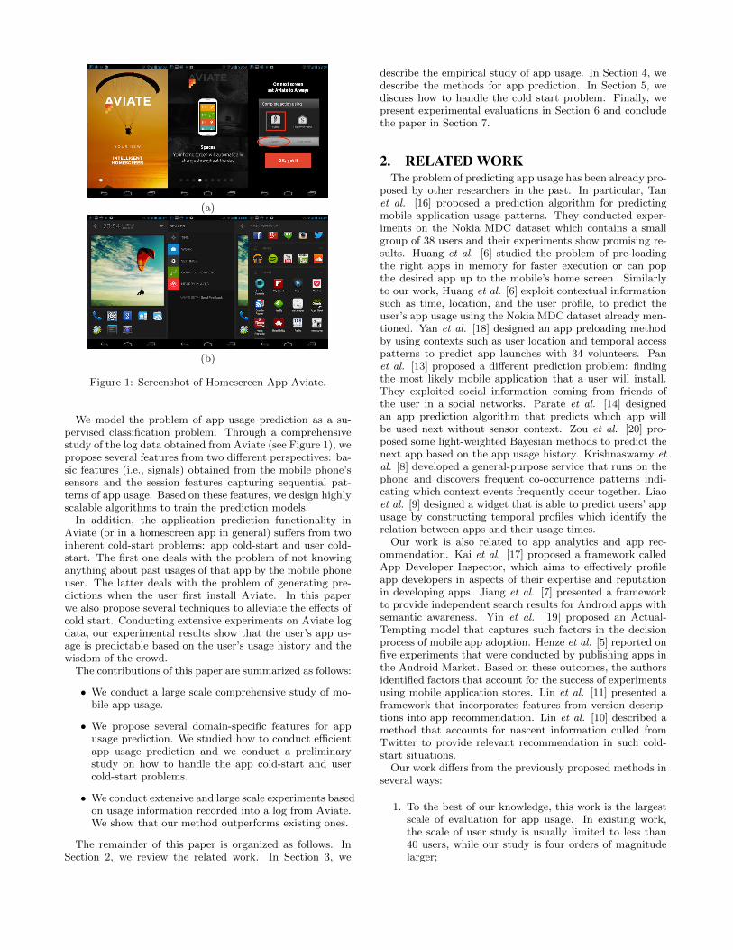
Figure 1: Screenshot of Homescreen App Aviate.

We model the problem of app usage prediction as a su-pervised classification problem. Through a comprehensivestudy of the log data obtained from Aviate (see Figure 1), wepropose several features from two different perspectives: ba-sic features (i.e., signals) obtained from the mobile phone’ssensors and the session features capturing sequential pat-terns of app usage. Based on these features, we design highlyscalable algorithms to train the prediction models.

In addition, the application prediction functionality inAviate (or in a homescreen app in general) suffers from twoinherent cold-start problems: app cold-start and user cold-start. The first one deals with the problem of not knowinganything about past usages of that app by the mobile phoneuser. The latter deals with the problem of generating pre-dictions when the user first install Aviate. In this paperwe also propose several techniques to alleviate the effects ofcold start. Conducting extensive experiments on Aviate logdata, our experimental results show that the user’s app us-age is predictable based on the user’s usage history and thewisdom of the crowd.

The contributions of this paper are summarized as follows:

• We conduct a large scale comprehensive study of mo-bile app usage.

• We propose several domain-specific features for appusage prediction. We studied how to conduct efficientapp usage prediction and we conduct a preliminarystudy on how to handle the app cold-start and usercold-start problems.

• We conduct extensive and large scale experiments basedon usage information recorded into a log from Aviate.We show that our method outperforms existing ones.

The remainder of this paper is organized as follows. InSection 2, we review the related work. In Section 3, we

describe the empirical study of app usage. In Section 4, wedescribe the methods for app prediction. In Section 5, wediscuss how to handle the cold start problem. Finally, wepresent experimental evaluations in Section 6 and concludethe paper in Section 7.

2. RELATED WORKThe problem of predicting app usage has been already pro-

posed by other researchers in the past. In particular, Tanet al. [16] proposed a prediction algorithm for predictingmobile application usage patterns. They conducted exper-iments on the Nokia MDC dataset which contains a smallgroup of 38 users and their experiments show promising re-sults. Huang et al. [6] studied the problem of pre-loadingthe right apps in memory for faster execution or can popthe desired app up to the mobile’s home screen. Similarlyto our work, Huang et al. [6] exploit contextual informationsuch as time, location, and the user profile, to predict theuser’s app usage using the Nokia MDC dataset already men-tioned. Yan et al. [18] designed an app preloading methodby using contexts such as user location and temporal accesspatterns to predict app launches with 34 volunteers. Panet al. [13] proposed a different prediction problem: findingthe most likely mobile application that a user will install.They exploited social information coming from friends ofthe user in a social networks. Parate et al. [14] designedan app prediction algorithm that predicts which app willbe used next without sensor context. Zou et al. [20] pro-posed some light-weighted Bayesian methods to predict thenext app based on the app usage history. Krishnaswamy etal. [8] developed a general-purpose service that runs on thephone and discovers frequent co-occurrence patterns indi-cating which context events frequently occur together. Liaoet al. [9] designed a widget that is able to predict users’ appusage by constructing temporal profiles which identify therelation between apps and their usage times.

Our work is also related to app analytics and app rec-ommendation. Kai et al. [17] proposed a framework calledApp Developer Inspector, which aims to effectively profileapp developers in aspects of their expertise and reputationin developing apps. Jiang et al. [7] presented a frameworkto provide independent search results for Android apps withsemantic awareness. Yin et al. [19] proposed an Actual-Tempting model that captures such factors in the decisionprocess of mobile app adoption. Henze et al. [5] reported onfive experiments that were conducted by publishing apps inthe Android Market. Based on these outcomes, the authorsidentified factors that account for the success of experimentsusing mobile application stores. Lin et al. [11] presented aframework that incorporates features from version descrip-tions into app recommendation. Lin et al. [10] described amethod that accounts for nascent information culled fromTwitter to provide relevant recommendation in such cold-start situations.

Our work differs from the previously proposed methods inseveral ways:

1. To the best of our knowledge, this work is the largestscale of evaluation for app usage. In existing work,the scale of user study is usually limited to less than40 users, while our study is four orders of magnitudelarger;

Table 1: Examples of Aviate Log Data (the user ID is anonymized to ensure privacy).

User ID App Action

xx8ae648c10 ”ts”:”2014-01-10 12:27:39”,”et”:”App Opened” [”com.skype.raider”]xx8ae648c10 ”ts”:”2014-01-10 12:36:09”,”et”:”App Opened” [”com.android.dialer”]xx8ae648c10 ”ts”:”2014-01-10 12:47:41”,”et”:”Location Update” [”37.393093”,”-122.079788”,”20.000000”,”0.000000”]xx8ae648c10 ”ts”:”2014-01-10 12:57:42”,”et”:”Context Triggered” [”Work”]

2. We achieve the highest precision for app prediction.The precision of the state-of-the-art is usually far be-low 90%;

3. Besides achieving high precision, our method is highlyscalable for big data;

4. We study the cold start problems that are still open inapp usage prediction and we study both perspectivesof cold start: users and apps.

3. APP USAGE CHARACTERIZATIONAs this is the first time that such a large scale analysis is

performed, we present here some basic statistics of the Avi-ate sample log data. The log sample contains more than 60million records with about 200K anonymized users that havea total of more than 70K unique apps by January 2014. Anexample of the events recorded in the log are shown in Ta-ble 1. For example, the first log entry indicates that “Skype”(the app) com.skype.raider was opened by user xx8ae648c10at 2014-01-10 12:47:39. The third entry shows that theuser’s location is moved to the GPS location (37.393093, -122.079788). The fourth entry tells us that Aviate’s workingmode is switched to Work.

Aviate records 10 types of actions in total. The distribu-tion of those actions is depicted in Figure 2. As expected,App Open represents a large fraction of app actions. Thisactually confirms that the app prediction problem could im-pact significantly on Aviate by improving its user experience.Furthermore, we observe that the fraction of App Installedevent is relatively low but is non-negligible (around 250Ktimes in our dataset). Just to put this into perspective ev-ery ten times a user changes location he or she installs anapp. For this reason the app cold-start problem is an im-portant one that needs a particular attention.

Figure 2: Distribution of Actions.

4. APP USAGE PREDICTIONIn this section we discuss the problem of predicting the

next app that a given user is going to open as she will pick upher mobile phone. We start by presenting a naive predictionstrategy based on apps popularity in 4.1. We discuss our setof features, namely basic and session features in Sections4.2 and 4.3, respectively. Then we discuss how to train theprediction model and how to generate predictions in Section4.4.

4.1 Predictions by PopularityAt first sight the app prediction problem might seem to

be straightforwardly solvable by always predicting the mostpopular app. While it is obvious that a popularity scorecomputed globally among all the users is not going to workin practice, it might seem reasonable to consider a per-userpopularity score. We discuss two kinds of popularity-basedfeatures: Global Frequency and Timeslot Frequency. GlobalFrequency represents the number of times that an app hasbeen opened by a particular user. Timeslot Frequency, in-stead, is the number of times that an app has been openedwithin a specific timeslot of the day (e.g. at Noon). Weconsider timeslots of granularity ranging from 1 day to 1second and based on the two kinds of frequencies we predictthe next app by selecting the one with the highest (globalor timeslot-based) popularity. We run a test to evaluatethe effectiveness of popularity-based approaches. We ex-tract popularity statistics on 80% of the log data and wetest the methods on the remaining 20%. Results show thatusing Global Frequency we can achieve an average precisionof up to 16.7%. We observe similar results also when we con-sider timeslot-based statistics. Results of predictions usingvarious timeslot granularities are shown in Figure 3. Us-ing 1 day based timeslots we reach a precision of 16.3%.Reducing the timeslot to 1 hour the prediction precision de-creases to 15.2% and the precision further decreases to 12.6%when the timeslot size is 1 second. Results shown in Fig-ure 3 demonstrate that differently from what the intuitionsuggests, solely relying on timeslots is not effective to findany useful pattern in real-life app usage scenarios. We fur-ther investigate the prediction performance of considering aweek as a cycle. We calculate the frequencies of each appat each day in a week and using the most frequent one atthe corresponding date. The prediction precision is 10.5%showing that app usage does not have very strong periodicphenomenon in terms of week.

In order to understand why popularity-based predictionmight fail, we study the distribution of the activeness of theapps, in other words how an app is used. The activenessof an app a is denoted as ∆a, which is formally defined asfollows:

∆a =

∑Si=1

FaiFi

S,

Figure 3: App Usage Prediction by Timeslot Frequency.

where S is the number of timeslots, Fai is the frequency ofa in timeslot i and Fi is the frequency of all apps in the i-thtimeslot. ∆a reflects a’s activeness across different timeslotsin each day. We show app activeness with its activeness rank(in decreasing order of activeness) for the 30 most popularapps in Figure 4. In the plot each line corresponds to a dif-ferent timeslot granularity. We find that the activeness ofthe apps on mobile device follows a power-law distribution.A small fraction of dominant apps take a large proportionof the whole activeness. Most of these dominant apps arerelated to basic services like browser, phone and communi-cation. These dominant apps are frequently used in eachtimeslot, making the other apps hard to predict if only thefrequencies are considered. Hence, we need to look for moreeffective features to approach the problem.

Figure 4: Activeness Proportion v.s. Activeness Rank

4.2 Basic FeaturesSince app usage is strongly related to the user’s spatiotem-

poral context, we discuss some basic features that can bedirectly obtained from the sensors of mobile devices. Thesebasic features defining the user’s spatiotemporal contexts arethe following: Time, Latitude, Longitude, Speed, GPS Accu-racy, Context Trigger Context Pulled, Charge Cable, AudioCable. The first five features are self-explanatory. ChargeCable and Audio Cable indicate whether the correspondingcable is plugged into the mobile device. Context TriggerContext Pulled indicate whether the corresponding Aviate

user has switched the ambient in which he operates (e.g.,“work”, “home”, etc). Among these features, only contexttrigger and context pulled are peculiar of Aviate whereasthe other features are obtained from the OS. These featureshelp to represent the spatiotemporal context of actions re-lated to the app open event. The feature Time is normalizedbetween 00:00:00-23:59:59, in order to capture daily app us-age patterns. As a side note, we have also tried to add theApp Activeness feature to our set of basic features. Thecontribution of avtiveness has not been significant thereforewe have removed it and we are not going to consider it inthe experiments we show next.

4.3 Session FeaturesBasic features do not capture latent relations between app

actions. Intuitively, and as also reported by Huang et al. [6],the correlation between sequentially used apps may have astrong contribution to the accuracy of app prediction. Inthis section we propose a method to extract session featuresby considering the sequential relationships existing amongapp actions.

We exploit the ideas presented in word2vec [12]. Inword2vec documents are modeled as sequences of terms anda context of a term is defined to be the k immediatelypreceding and following terms in the document. Likewise,we model documents with sequences of app events but wecannot simply choose the preceding and following actionsas the context of an app given that they may be associ-ated with events happened a long time back in the past(or ahead in the future). Based on this observation, wepropose a Gaussian based method to identify the contextof each app action. The context is defined as the set ofother actions that are conducted before or after the cur-rent one within a time period whose duration is obtainedby sampling from an empirically defined Gaussian distribu-tion. For example, in Table 1 we show a context relative toApp Open:com.android.dialer formed by the following twoapp actions: App Open:com.skype.raider, and Location Up-date:(37.393093, -122.079788, 20.000000, 0.000000).

Our objective is to find distributed representations ofthese features that are useful for predicting the surround-ing actions of the current context. More formally, given anapp action τ and its context Cτ , the objective is to maximizethe average log probability:

1

T

T∑t=1

∑τ ′∈Ct

log p(τ ′|τt), (1)

where Ct is the context of τt and T is the number of appactions. The probability p(τ ′|τt) is calculated as follows:

p(τ ′|τt) =eVτ′ ·Vτt∑Tt=1 e

Vτ′ ·Vτt(2)

where Vτ ′ is the distributed representation of τ ′ and Vτt isthe distributed representation of τt.

In order to enhance the efficiency, the full softmax inthe above formula is approximated by the hierarchical soft-max [12]. In order to efficiently compute the distributedrepresentations, we parallelize the training procedure usinga MapReduce paradigm. The Mapper and Reducer are pre-sented in Algorithms 1 and 2. The MapReduce procedureiterates for a predefined number of times and the outputvectors are the session features for mobile apps.

Algorithm 1 Mapper of Distributed Representation

1: load the vectors of app actions from the previous iteration;2: initialize the Huffman tree based on the loaded vectors;3: for each app action a do4: draw a temporal gap g1 from Gaussian distribution G;5: draw a temporal gap g2 from Gaussian distribution G;6: consider the actions between g1 and g2 as the context Ca;7: train a based on Ca;8: end for9: for each app action action a do

10: emit(key=IDa,value=V ectora);11: end for

Algorithm 2 Reducer of Distributed Representation

1: for each app action a do2: calculate average and normalize the corresponding vectors;3: end for4: flush updated vectors to HDFS;

Based on Algorithms 1, and 2, we define distributed repre-sentations of the following six app actions: Last App Open,Last Location Update, Last Charge Cable, Last Audio Ca-ble, Last Context Trigger, Last Context Pulled. The corre-sponding distributed representations of the six actions arein turns considered as the session features for the app pre-diction method we use.

4.4 Building Prediction ModelsBy merging basic and session features for each App Open

event, we obtain the training instances for the predictionmodel. In order to achieve a balance between effective-ness and efficiency, we propose the Parallel Tree AugmentedNaive Bayesian Network (PTAN) as the prediction model.PTAN is a parallel version of the Tree Augmented NaiveBayes (TAN) [3], which has been proposed in order toremove the strong assumptions of independence in nativeBayes and exploit the correlations among attributes. Thismodel captures the latent correlations between different fea-tures and can be easily deployed on parallel computingframeworks such as Hadoop. The training procedure ofPTAN can be divided into two phases: (1) parallel struc-ture training and (2) parallel parameters estimation. Thefirst phase is to learn the structure of the Bayesian network.The procedure of constructing the PTAN bayesian networkfrom data is as follows:

1. Based on the training data from all users, we com-pute the conditional mutual information between anytwo attributes fx and fy given the app a. Conditionalmutual information is defined as follows:

Ip(fx, fy|a) =∑

fx,fy,a

P (fx, fy, a) logP (fx, fy|a)

P (fx|a)P (fy|a).

2. Build a complete undirected graph in which the ver-tices are the features. Annotate the weight of an edgeconnecting feature fx and fy by Ip(fx, fy|a).

3. Build a maximum weighted spanning tree for the com-plete undirected graph. The maximum spanning treeproblem can be transformed to the minimum span-ning tree problem simply by negating edge weights [2].Kruskal’s algorithm [4] is used to solve the minimumspanning tree problem.

4. Transform the resulting undirected tree to a directedone by choosing a root variable and setting the direc-tion of all edges to be outward from it. Construct aBayesian network by adding a vertex labeled by appvariable a and adding an arc from a to each featurevertex.

The highest computational cost is associated with the firstand the third step in the above algorithm. If we assume thereexist m training instances and each instance has n featuresthen the first step has complexity of O(n2m). The thirdstep has a complexity of O(n2 logn). Since m logn, thefirst step is the bottleneck of building the Bayesian networkstructure. Hence, in PTAN, we parallelize the first stepagain using MapReduce. The Mapper for parallelizing thefirst step is presented in Algorithm 3 and the Reducer can bestraightforwardly developed by aggregating the values basedon the keys.

Algorithm 3 TAN Structure Learning Mapper

1: for each app action entry u, a, f1, f2, f3, ..., fn do2: for each feature pair (fi, fj) do3: emit(key=fi, fj , a,value=1);4: emit(key=fi, a,value=1);5: emit(key=fj , a,value=1);6: end for7: end for

After learning the structure of PTAN, we estimate a setof parameters for each individual user, in order to achievethe personalization effect. The conditional probability isestimated as follows:

P (fi = k|pa(fi) = j) =Nijk +N ′ijkNij +N ′ij

, (3)

where fi is a feature, pa(fi) is the set of the parents of fi,Nij is the number of times pa(fi) = j, Nijk is the num-ber of times fi = k given pa(fi) = j in the training set,and N ′ij and N ′ijk are the smoothing parameters that we setboth to 0.5 by default. Smoothing is fundamental for theprediction performance when some user contains very fewtraining instances for an app. Furthermore, parameters es-timation for each user is also parallelized. The Mapper ispresented in Algorithm 4 and the Reducer can be straight-forwardly developed by aggregating the values based on thekeys. When the parameters for the Bayesian network havebeen estimated we compute the probability that a user u isgoing to use mobile app aui when it finds herself within thecontext C = f1, f2, ..., fn as follows:

P (aui|f1, f2, ..., fn)

∝ P (aui)P (f1, f2, ..., fn|aui)

= P (aui)

n∏i=1

P (fi|pa(fi))

(4)

Based on this equation we consider the app that has thehighest probability as the prediction result. It is straight-forward to transform this prediction algorithm into a top-krecommendation one just by sorting apps according to thecomputed probability scores.

Algorithm 4 TAN Parameter Learning Mapper

1: for each action long entry u, c, a1, a2, a3, ..., an do2: for each pair

(ai, pa(ai)

)do

3: emit(key=ai, pa(ai),value=1);4: emit(key=pa(ai),value=1);5: end for6: end for

5. COLD START PROBLEMSIn this section, we discuss how to handle two of the main

challenges we face when homescreen apps that are deployedin real-life environments. The first problem is the App ColdStart, which happens when a user installs a new app on herdevice. The second problem is the User Cold Start thatarises when a user installs and open the homescreen appfor the first time. User cold start is more severe than thefirst one given that in order to reduce the risk of app aban-donment it is important to provide high quality personal-ized predictions already from the first interactions with thehomescreen app. We discuss how to tackle these two coldstart problems in Sections 5.1 and 5.2.

5.1 App Cold StartFor a newly installed app ai, we have no user-specific in-

formation available on the app. In particular the probabilityof opening an app for a given user u, P (aui), is unavailable.On the other hand, P (fi|pa(fi)), the prior probability fora given feature, can be obtained from information on otherusers. Therefore, for newly installed apps, how to estimateits P (aui) is critical. We present the app activeness for newlyinstalled apps in Figures 5 (Daily) and 6 (Hourly). We cansee that a significant fraction of the newly installed apps isvery active within the first few hours. After this period oftime the newly installed apps are used significantly less. Incontrast, some apps are used frequently and for a long timeafter their installation. Hence, in order to better estimateP (ai), we categorize apps as short-term apps and long-termapps depending on their activeness longevity.

In order to capture the temporal prominence of each appwe fit app usage data into a Beta(α, β) variable and to dif-ferentiate apps by their temporal significance we use theexcess kurtosis [15] to evaluate the temporal peakedness ofeach app. The excess kurtosis % of a Beta(α, β) distributionis defined as follows:

% =6[α3 − α2(aβ − 1) + β2(β + 1)− 2αβ(β + 2)]

αβ(α+ β + 2)(α+ β + 3). (5)

An app with a high % value indicates that it is likely to bea short-term app while an app with a low % value is likelyto be a long-term app. Through using %, we can categorizethe apps into short-term apps and long-term app. Table 2shows some examples after categorization. As an example,we can observe that while communication apps are usuallylong-term game apps tend to have a shorter life span.

Short-term App. We assign to short-term apps a P (aui)value of P (ai), which is the average opening frequency ob-tained from other users’ historical information. After a fixedtime period (two hours, for example) we can replace P (ai)with the actual app’s usage information for that particularuser, namely P (aui).

Long-term App. For long-term apps, we exploit thewell-known concept of “wisdom of the crowd”. When an

Figure 5: Daily App Activeness (Proportion) After Instal-lation.

Figure 6: Hourly App Activeness (Proportion) After Instal-lation.

app has been opened very few times its P (ai) should ap-proximate the average value coming from other users. Asthe number of open events grow we can switch to the actualP (aui). Hence, we used Bayesian average [1] to effectivelyblend actual usage information with that coming from otherusers’ history. The equation for calculating P (aui) is there-fore given by:

P (aui) =C · Ωai + Oaui

C + Ou, (6)

where Oaui is the number of openings of the app ai by thecurrent user U , Ou is the sum of all app openings by u,and Ωai is the average opening probability of ai by all otherusers. C is a constant whose value is set to match the ex-pected variation between data sets containing the historyfrom different users. The value of P (aui) for an app witha small number of open events tends to be closer to theaverage opening probability of that same app by all otherusers. The more openings an app has received by the cur-rent user, the more accurate the probability estimation is.

Table 2: Examples of Short-term and Long-term Apps.

Short-term Appsjp.gree.jackpot

com.rockstargames.gtasacom.sq.dragonsworld

com.cocoapps.elbombermancom.zhan dui.animetaste

com.sweettracker.smartparcelcom.mobie.catholiclife

com.partyplay.xxlcom.king.candycrushsaga

com.battlelancer.seriesguideLong-term Appscom.quixey.android

com.google.android.talkcom.whatsapp

mobi.mgeek.TunnyBrowsercom.fitbit.FitbitMobile

com.spotify.mobile.android.uicom.google.android.apps.authenticator2

com.facebook.katanacom.myfitnesspal.androidcom.google.android.gm

On the other hand, when an app has received just a smallnumber of openings, its estimated P (aui) value is close toits unweighted average opening probability computed on allthe other users.

5.2 User Cold StartIn this subsection, we discuss two different strategies to

tackle the user cold start problem. In Section 5.2.1 we dis-cuss the Most Similar User Strategy essentially based on col-laborative filtering. In Section 5.2.2 we discuss the PseudoUser Strategy that is designed to synthesize an appropriatepseudo-history for the new user so that the PTAN modelcan be effectively trained on this surrogate usage data.

5.2.1 Most Similar User StrategyWhen a new user installs homescreen apps such as Aviate,

it is not true that we do not know anything about her. Inparticular, we know her apps inventory and using this infor-mation we can identify the most similar user from the set ofknown users by using metrics such as, for instance, Jaccardsimilarity between the new user and the known ones.

After the most similar user has been found, we can use thisuser’s model to predict the behavior of the new user. Wename this strategy as the Most Similar User Strategy. Infact, the most similar user may have an app inventory thatis very different from that of the user under consideration. Insome extreme cases the app inventory can be totally differentfrom those installed by known users and the most similaruser strategy would not have any sensitive advantage overa purely random strategy. Of course we can resort to puta threshold on the minimum acceptable similarity. Whilethis strategy improves the average accuracy of the methodit also limits the coverage, i.e., the number of users for whichrecommendations can be generated.

5.2.2 Pseudo User StrategyIn order to solve the problem of the strategy presented

above we propose the Pseudo User strategy, which consistsin generating a “pseudo history” used in place of the actualone to train the PTAN model for the new user. Let usassume there are k users U = u1, u2, u3, ..., uk and letus further assume that each user u has an app inventoryIu. When a new user with app inventory Inew installs thehomescreen app, we obtain I ′u for each u by only keeping theapps in Inew. We want to find a subset of users U ′ satisfyingthe following conditions:

min∑u∈U′

|c(u)|

subject to⋃u∈U′

I ′u = Inew .

The cost of an user c(u) is defined as the inverse of its sim-ilarity to the current user, i.e., c(u) = 1/J(Inew, Iu). Theidea is to find a small amount of similar users whose app in-ventories cover all the apps in the inventory of the new user.It is straightforward to prove that the problem is NP-hard(it is essentially a weighted set-covering problem) and theO(log |Inew|)-approximation algorithm we use to generatethe pseudo user is presented in Algorithm 5. After obtain-ing U ′ we aggregate log entries for each user in U ′ and wefilter out the App Open events for those apps that are notin Inew. What it is left is considered to be the Pseudo Userdata used in PTAN training.

Algorithm 5 Building Pseudo User

1: U ′ ← ∅2: I ← ∅3: repeat

4: choose u ∈ U minimizingc(u)

|I∪Iu−I|5: let U ′ ← U ′ ∪ u6: let I ← I ∪ I′u7: until I = Inew

6. EXPERIMENTSIn this section we measure the performance of the pro-

posed method. Experiments are conducted on Aviate logdata collected from October 2013 to April 2014. We ran-domly choose 480 active Aviate users for our experiments.For each user, we use 80 percent of the data as trainingdata and the remaining 20 percent as testing data. For allthe methods we extract features (both basic and session)using events within a sliding window of 12 hours, as we as-sume that any event only influence future events that hap-pen within 12 hours. In Section 6.1 we measure the perfor-mance of the propose app prediction algorithm. In Sections6.2 and 6.3, we evaluate the performance of our solution tothe app and user cold start problems, respectively.

6.1 App Usage PredictionAs we have stated in the previous sections, we modeled

the app prediction problem as a classification problem andwe opted for a parallelized version of the Tree AugmentedNaive Bayes (TAN) algorithm to build the classifier. In or-der to assess the effectiveness of PTAN we compare it withthe best ML algorithms that are suitable for this problem,namely Naive Bayes, SVM, C4.5, and Softmax Regression

(i.e., Multinomial Logistic Regression). In the experimentswe report the score for precision, that is the percentage ofcorrectly predicted opened apps over the total number ofapp opened by users in the test data.

Figure 7 shows the performance of different methods inthe case of a model trained when the context is made upof only the basic features. In this case, C4.5 achieves thehighest precision of 34.9%. We investigated the reasons whyC4.5 results is the best method for basic features and weconjecture that is due to that some apps have a very clearfingerprint in terms of sensor usage that a classification treeis able to surface. For example, by analyzing the decisiontree, we found that when the charge cable is plugged in, thepredicted apps were some video games or using bluetooth.Intuitively, game apps or file transmission apps usually con-sume more battery energy, therefore when you plug yourcharge cable (and you do not wait too much time beforetaking an action), it is very likely you are going to use oneof the two classes of applications mentioned above.

We then evaluate the hypothesis we made that sequence-based patterns are useful for building more effective clas-sifiers. For methods such as Naive Bayes, C4.5, PTANand Softmax Regression, the session features are effective toboost the performance. Therefore, these results confirm theassumption that the sequential correlations between app ac-tions are critical for app usage prediction. Combining basicfeatures and session features is an effective strategy for Bayesmethods. With both types of features, Naive Bayes achievesa precision of 76.3% and PTAN achieves the highest preci-sion of 90.2%. We also studied the impact of dominant apps(i.e, the most frequent apps) in app prediction. By filteringthe top five dominant apps for each user, we reevaluate theperformance of the five methods. The performance of NaiveBayes with basic and session features is heavily influenced,giving a precision of 39.3%. Among the five methods, PTANstill achieves the highest precision of 85.7% with all the fea-tures. Therefore, we can conclude that while dominant appsare easy to predict using even just a Naive Bayes classifier,when they are removed a strong signal can still be obtainedby opportunely combining the other features we have de-signed (in particular features about event sequences).

Figure 7: App Usage Prediction (All Apps).

Figure 8: App Usage Prediction (Dominant Apps Filtered).

In order to comprehensively measure the performance ofthe proposed method, we compare it with the state-of-the-art counterparts. Although some methods described in Sec-tion 2 are related to our work, some of them are not com-parable with PTAN because they use some additional infor-mation. We select EWMA [16], CPD [16], LU-2 [20], LUT[20], and BN [20] as comparison baselines as they can beused on our dataset. We evaluate these baselines by vary-ing the different values of the parameters that characterizethose methods. Figure 9 shows the performance of EWMAand CPD on the full set of apps (including dominant ones)and Figure 10 shows the performance of EWMA and CPDwhen dominant apps have been filtered out from the dataset.With the full set of apps EWMA achieved the highest pre-cision of 16.7%. When dominant apps were filtered out, in-stead, CPD has a precision of 19.5%, which is the highest inthis case. We further observe that EWMA performs betterwith all apps while CPD performs better when the domi-nant apps are filtered. Figure 11 shows the performance ofLU-2, LUT and BN. LU-2 shows the best performance withall apps, achieving a precision of 15.7% while BN achievesthe highest precision of 10.1%.

From the various results shown we can conclude thatPTAN significantly outperforms the five baselines we con-sider by a large margin. We remark that the experimentsdone using the techniques presented in the papers describingthe baselines were done on a much smaller dataset contain-ing usage data on 38 users in total. Our user set is oneorder of magnitude larger while the dataset is several orderof magnitude larger. Nevertheless the performance reportedfor papers on the baselines methods are consistent with theones we report here.

6.2 App Cold StartWe now assess the performance of the method discussed

in Section 5.1 and we evaluate its effectiveness in alleviatingthe app cold start problem. For each app installment, weprocess the original dataset by splitting it into two subsets:one subset containing all the events referred to the periodbefore the app installment and one subset containing the re-maining events. We then build a model for predicting appopening events contained in the second file by using events

Figure 9: App Usage Prediction of Baselines (All Apps).

Figure 10: App Usage Prediction of Baselines (DominantApps Filtered).

in the first file. For short-term apps (those that are heavilyused in the moments immediately following their installa-tion), the precision of app prediction improves from 86.3%1

to 87.1% after applying the strategy described in Section 5.1.In particular the precision for new apps is about 91.3% andfor existing apps is about 86.25%. The prediction qualityfor existing apps is thus not heavily hurt. The results con-firm that in the case of short-term apps we usually observeopening events during the first day after they are installed.The number of opening events steadily decreases afterwards.Therefore, assigning a relatively high probability for theseapps is useful for improving the performance. Note thatthe increase in precision is significant since users open manyapps each day and the opening of the newly installed appsmay only happen in a relatively small fraction of the cases.Indeed, the percentage of newly installed apps in the testdata is only 1.42%.

The precision we measure in the case of long-term appsis 89.3% when we use the general method, but no newly

1Precision percentages are different from the previous sec-tion as we are reporting results on a different partitioning ofthe dataset created to test cold start methods.

Figure 11: App Usage Prediction of Baselines.

installed app is correctly predicted in this case. By apply-ing the proposed cold-start strategy the precision measuredincreases up to 90.3% on average. More accurately the pre-cision is 91.1% for new apps and 89.26% for existing apps,also confirming that in this case the precision on existingapps is not heavily hurt.

6.3 User Cold StartExperimental results show that the Most Similar User

Strategy achieves an average precision of 32.7%. We presentthe correlation between app inventory similarity and appprediction precision in Figure 12. We observe that the appinventory is useful yet not very effective. There are two mainreasons that may explain this result. First, it is not easy tofind a user with highly similar inventory. In our dataset,the Jaccard similarity between two different app invento-ries is typically low. We found an average value of 0.121465(±0.038955) and a median of 0.117647. Second, even whenthe similarity is high the corresponding precision increase isnot always satisfactory. In many cases, we observe that theprecision is almost zero even when similarity of the two appinventories is relatively high.

Figure 12: App Prediction By Similar User.

On the other hand, the average precision of the PseudoUser Strategy is 45.7%. Therefore we confirm that estimat-ing usage data about apps in a new user inventory using thisstrategy is effective to boost the performance of the predic-tion model.

Besides reporting the effectiveness of the two proposeduser cold start strategies we also studied after how manydays the app prediction model can achieve acceptable pre-diction precision. The result is presented in Figure 13 wherewe show that even after just one single day of data about theuser has been collected the prediction’s precision increasesup to more than 56%. Precision further increases up to81.5% when two days of historical data are considered.

We can conclude that Most Similar User Strategy andPseudo User Strategy are both useful but only in the verysame day the homescreen app has been installed. After that,for a typical user, high-precision prediction models can betrained using the real (i.e., collected) usage data from thatuser.

Figure 13: App Prediction Precision v.s. Number of Days.

7. CONCLUSIONSIn this paper we have proposed a new methodology to

predict what is the next mobile app that a user is going toopen. We conducted a comprehensive analysis on a verylarge scale mobile log containing events recorded by Aviate,the Yahoo’s homescreen app. We proposed a set of basicand session features that are designed to capture the se-quential correlation between different actions involving mo-bile apps; e.g., plugging the charging cable. Based on thesefeatures, we built a Parallel TAN model to efficiently solveour app prediction problem. We further studied how to al-leviate the app cold start problem and the user cold startproblem. We conducted a wide spectrum of experiments tostudy the parameter sensitivity and effectiveness of the pro-posed method. Experimental results demonstrated that appusage is predictable even though a naive strategy based onpopularity features fail to achieve high effectiveness. Theproposed method outperformed the state of the art by alarge margin.

In the future we plan to further improve the predictionperformance at cold start. In particular the problem to im-prove the performance of user cold start app prediction re-mains open. Regarding app cold start it is an open problem

that of optimizing the performance of the predictor in thepresence of a mix of cold and non-cold apps. Finally, it isrelated the problem of finding the top-k applications thata user would open instead of the next one. The problem,then, could be cast into a learning to rank rather than intoa classification one.

8. REFERENCES[1] George EP Box and George C Tiao, Bayesian inference in

statistical analysis, vol. 40, John Wiley & Sons, 2011.

[2] David Eppstein, Spanning trees and spanners, Handbook ofcomputational geometry (1999), 425–461.

[3] Nir Friedman, Dan Geiger, and Moises Goldszmidt, Bayesiannetwork classifiers, Machine learning 29 (1997), no. 2-3.

[4] John C Gower and GJS Ross, Minimum spanning trees andsingle linkage cluster analysis, Applied statistics (1969), 54–64.

[5] Niels Henze, Martin Pielot, Benjamin Poppinga, TorbenSchinke, and Susanne Boll, My app is an experiment:Experience from user studies in mobile app stores,International Journal of Mobile Human Computer Interaction(IJMHCI) 3 (2011), no. 4, 71–91.

[6] Ke Huang, Chunhui Zhang, Xiaoxiao Ma, and Guanling Chen,Predicting mobile application usage using contextualinformation, Proceedings of the 2012 ACM Conference onUbiquitous Computing, ACM, 2012, pp. 1059–1065.

[7] Di Jiang, Jan Vosecky, Kenneth Wai-Ting Leung, and WilfredNg, Panorama: A semantic-aware application searchframework, Proceedings of the 16th International Conferenceon Extending Database Technology, ACM, 2013, pp. 371–382.

[8] Shonali Krishnaswamy, Joao Gama, and Mohamed MedhatGaber, Mobile data stream mining: from algorithms toapplications, Mobile Data Management (MDM), 2012 IEEE13th International Conference on, IEEE, 2012, pp. 360–363.

[9] Zhung-Xun Liao, Po-Ruey Lei, Tsu-Jou Shen, Shou-Chung Li,and Wen-Chih Peng, Mining temporal profiles of mobileapplications for usage prediction, Data Mining Workshops(ICDMW), IEEE 12th International Conference on.

[10] Jovian Lin, Kazunari Sugiyama, Min-Yen Kan, and Tat-SengChua, Addressing cold-start in app recommendation: latentuser models constructed from twitter followers, Proceedings ofthe 36th international ACM SIGIR conference on Research anddevelopment in information retrieval, ACM, 2013, pp. 283–292.

[11] , New and improved: modeling versions to improveapp recommendation, Proceedings of the 37th internationalACM SIGIR conference on Research & development ininformation retrieval, ACM, 2014, pp. 647–656.

[12] Tomas Mikolov, Ilya Sutskever, Kai Chen, Greg S Corrado, andJeff Dean, Distributed representations of words and phrasesand their compositionality, Advances in Neural InformationProcessing Systems, 2013, pp. 3111–3119.

[13] Wei Pan, Nadav Aharony, and Alex Pentland, Composite socialnetwork for predicting mobile apps installation., AAAI, 2011.

[14] Abhinav Parate, Matthias Bohmer, David Chu, DeepakGanesan, and Benjamin M Marlin, Practical prediction andprefetch for faster access to applications on mobile phones,Proceedings of the 2013 ACM international joint conference onPervasive and ubiquitous computing, ACM, 2013, pp. 275–284.

[15] Gamini Premaratne and Anil Bera, Modeling asymmetry andexcess kurtosis in stock return data, Illinois Research &Reference Working Paper No. 00-123 (2000).

[16] Chang Tan, Qi Liu, Enhong Chen, and Hui Xiong, Predictionfor mobile application usage patterns, Nokia MDC Workshop,vol. 12, 2012.

[17] Kai Xing, Di Jiang, Wilfred Ng, and Xiaotian Hao, Adi:Towards a framework of app developer inspection, DatabaseSystems for Advanced Applications.

[18] Tingxin Yan, David Chu, Deepak Ganesan, Aman Kansal, andJie Liu, Fast app launching for mobile devices using predictiveuser context, Proceedings of the 10th international conferenceon Mobile systems, applications, and services, ACM, 2012.

[19] Peifeng Yin, Ping Luo, Wang-Chien Lee, and Min Wang, Apprecommendation: a contest between satisfaction andtemptation, Proceedings of the sixth ACM internationalconference on Web search and data mining.

[20] Xun Zou, Wangsheng Zhang, Shijian Li, and Gang Pan,Prophet: what app you wish to use next, Proceedings of the2013 ACM conference on Pervasive and ubiquitous computingadjunct publication, ACM, 2013, pp. 167–170.