predicting the leaf water potential of potato plants using

Volume 50 2008 CANADIAN BIOSYSTEMS ENGINEERING 7.1

Predicting the leaf water potentialof potato plants using RGB reflectance

R. Zakaluk1 and R. Sri Ranjan2*

1Civil Engineering Technology Department, Red River College, Winnipeg, Manitoba R3H 0J9, Canada; and 2Department of

Biosystems Engineering, University of Manitoba, Winnipeg, Manitoba R3T 5V6, Canada. *Email: [email protected]

Zakaluk, R. and Sri Ranjan, R. 2008. Predicting the leaf waterpotential of potato plants using RGB reflectance. CanadianBiosystems Engineering/Le génie des biosystèmes au Canada 50: 7.1-7.12. Existing plant water status measurements are impractical to meetreal time irrigation monitoring requirements. This research exploredthe use of artificial neural network (ANN) modeling of imagescaptured by a ground-based, five megapixel, RGB (red green blue)digital camera to predict the leaf water potential (ΨL) of field grownpotato plants. Leaf water potential, soil nitrate (N) content, andvolumetric water content were obtained along with digital images inrandomly selected sample plots. The images from all the plots wereradiometrically calibrated and then classified to isolate green foliagefrom soils, flowers, shadows, and senescent leaves. The RGB images,six image transformations, and nine vegetation indices weretransformed using principal components analysis (PCA). Findingsshowed a significant inverse linear relationship between soil N and leafreflectance in the G image band (r = -0.71, p = 0.003) and that theANN model input neuron weights with more separation between soil Nand ΨL were most important in predicting ΨL. For the ANN modelvalidation dataset, findings indicated that the measured and predictedΨL distributions were normally distributed (Wmeas = 0.97, p = 0.8, Wpred

= 0.95, p = 0.6), the means were not significantly different (t = -1.00,p =0.3), and the variances were equal (F = 0.14, p = 0.7). Based onthese results, the ground-based digital camera proved to be an adequatesensor for image acquisition and a practical tool for predicting ΨL ofpotato plants. Keywords: nitrate, IHS transformation, chromaticitytransformation, principal components, vegetation indices, remotesensing, artificial neural network, digital camera.

Les méthodes courantes de mesure de teneur en eau des plantessont inappropriées pour la gestion en temps réel des systèmesd’irrigation. Cette étude a exploré l’utilisation de la modélisation parun réseau neuronal artificiel d’images prises par une caméra digitalefixe RGB (rouge vert bleu) de cinq mégapixels pour prédire lepotentiel hydrique des feuilles (ΨL) d’un champ de plants de pommesde terre. Le potentiel hydrique des feuilles, la teneur en nitrate (N) etla teneur en eau du sol sur une base volumique ont été mesurés et desphotographies digitales ont été prises dans des parcelles sélectionnéesde manière aléatoires. Les images de toutes les parcelles étaientcalibrées sur le plan radiométrique pour ensuite être classifiées dans lebut d’isoler le feuillage vert du sol, des fleurs, des ombres et desfeuilles sénescentes. Les images RGB, six transformations d’images etneuf indices de végétation ont été transformés en utilisant l’analyse descomposantes principales (ACP). Les résultats ont démontré unerelation linéaire inverse entre la teneur en N du sol et la réflexivité desfeuilles dans la bande d’image G (r = -0,71, p = 0,003). Unepondération plus importante entre la teneur en N du sol et Ψet au niveaudu modèle neuronal d’intrant ‘ANN’ était plus importante pour laprédiction de ΨL. Pour les données obtenues avec le modèle ANNvalidé, les résultats ont indiqué que la distribution des valeursmesurées et prédites de ΨL avaient une distribution normale (Wmesur =

0,97, p = 0,8, Wpréd = 0,95, p = 0,6) ; les moyennes n’étaient pasdifférentes (t = -1,00, p =0,3) et les variances étaient égales (F = 0,14,p = 0,7). Considérant ces résultats, une caméra digitale fixe s’est avéréeêtre un senseur adéquat pour l’acquisition d’images et un outil pratiquepour prédire ΨL des plants de pommes de terre. Mots clés: nitrate,transformation IHS, transformation chromatique, composantesprincipales, indices de végétation, senseur à distance, réseau neuronalartificiel, caméra digitale.

INTRODUCTION

Water is essential for plant growth and sustenance. Accordingto Bowman (1989), a decrease in plant water content causes adecrease in stomatal conductivity that limits the uptake ofcarbon dioxide for photosynthesis. Problems for potato(Solanum tuberosum L.) producers are created because plantwater stress on potato inhibits photosynthesis and causes adecrease in total biomass and a decrease in both fresh and drymatter tuber yield (Costa et al. 1997; Gunel and Karadogan1998). The leaf water potential (ΨL), a measure of the negativepressure that exists within the leaf cells, can be used to measureplant water status. The negative pressure results from stomatalresistance which causes water to flow from the roots toward theleaf. The dynamic nature of plant water status over a given 24-hperiod (Scholander et al. 1965; Waring and Cleary 1967),however, makes in situ plant water status measurementimpractical for irrigation scheduling over large areas.

Remote sensing either by airborne or spaceborne imageacquisition methods is a tool with the potential to monitor plantwater status over large areas (Bastiaanssen and Bos 1999;Jackson et al. 2004; Karimi et al. 2005). Previous researchadvocates the use of the short wave infrared (SWIR) region tomodel plant water content (Ceccato et al. 2002a, 2002b; Ripple1986). However, the addition of an imaging sensor in the SWIRwater absorption regions for vegetation at 1450, 1950, and2600 nm (Ustin 2004) to an irrigation scheduling system wouldbe cost prohibitive. Imaging sensors that model plant waterstatus in the visible region would therefore be moreeconomically viable for an irrigation scheduling system.Justification for using visible light reflectance as an indicator ofplant water status is based on the interrelationships betweenplant water status, photosynthesis, and irradiance load on theleaf (Carter 1991; Schlemmer et al. 2005; Wheeler 2006).Zakaluk and Sri Ranjan (2007) found that an RGB (red greenblue) digital camera could determine ΨL under greenhouseconditions. The objective of this study was to explore the use ofa digital camera to acquire images, in the visible region, of afield grown potato crop under different plant water levels anddifferent soil nitrate conditions.

LE GÉNIE DES BIOSYSTÈMES AU CANADA ZAKALUK and SRI RANJAN7.2

Changes in nitrogen and water availability result inphysiological changes in the plant that alter leaf reflectance inthe visible region (Penuelas et al. 1994; Schlemmer et al. 2005;Zhurmar and Yanovskaya 1992). Specifically, soil or plantnitrogen levels are associated with plant greenness (Blackmer etal. 1994; Boegh et al. 2002; Osborne et al. 2002; Schlemmer etal. 2005; Thomas and Oerther 1972). In addition, plant nitrogenlevels are associated with chlorophyll content (Haboudane et al.2002; Schlemmer et al. 2005). Plant nitrogen levels are alsorelated to the light energy incident upon the leaf surface andphotosynthesis (Charles-Edwards et al. 1986). Since soil andplant nitrogen interacts with chlorophyll content,photosynthesis, and reflectance in the visible spectral regionresearch, exploring leaf reflectance in the visible region todetermine ΨL must consider nitrate (N) levels in either the soilor plant.

To solve the problem of measuring plant water status forirrigation using remote sensing, an economical sensor with rapidimage delivery and flexible revisit rates must be employed.Commercially available digital cameras are one possiblesolution to meeting the requirements of applying remote sensingfor measuring plant water status using leaf reflectance in thevisible region. In this study, therefore, using a camera equippedwith a single five megapixel full frame sensor, RGB digitalimages were explored to determine the ΨL of field grown potato(Solanum tuberosum L. var. cv. Sangre) using artificial neuralnetwork (ANN) modelling under different soil N levels. Thefollowing questions were addressed:

1. Can 0.91 mm spatial resolution RGB images separatefoliage from shadow, soils, leaf senescence, and flowers?

2. Is there a relationship between soil N and leaf reflectance inthe green image band?

3. Can ANN modelling of RGB images determine ΨL ofpotatoes (Solanum tuberosum L. var. cv. Sangre) under fieldconditions?

4. Are there relationships between ΨL and soil N that influencethe relative importance of the input neurons in the ANNmodel?

5. Can a ground-based digital camera supply RGB images asan alternative to airborne-spaceborne imaging sensors?

METHODS

Agronomic instruments and measurements

A pressure chamber instrument (PMS Model 600, PMSInstrument Company, Albany, OR) was used to collect leafwater potential, ΨL (MPa). Soil N (0-150 mm) was determinedusing a hand-held Nitrachek™ 404 Reflectometer (KPGProducts Ltd., Hove, East Sussex, UK) and Merkoquant® N teststrip (Merck KGaA, Darmstadt, Germany) using the methoddescribed by Tremblay et al. (2001).

Imaging sensor and platform

A five megapixel, single, charged couple device (CCD) chip,Sony DSC-T1 digital full frame camera using a 35-mm cameraequivalent focal length of 38 mm, capturing 2592 x 1944 pixelimages, was used to acquire images. The size of each detectoron the CCD chip was 2.775 x 2.775 µm. The peak wavelengthswere empirically determined to be 610, 520, and 460 nm for theR, G, and B filters, respectively (Sony Corporation 2004). Thedigital camera was operated by remote control and mounted ona telescopic pole that extended 2.5 m above ground level (AGL)covering 2.37 x 1.78 m on the ground. The ground spatialresolution of each pixel was 0.91 x 0.91 mm.

Experimental design

Data were collected in a 29-ha field (Fig. 1) locatedapproximately 130 km southwest of Winnipeg, Manitoba (490

16.198' N, 980 3.146' W) during cloud free periods. In theprevious fall, nitrogen fertilizer was not applied to the field. Thefield consisted of coarse-loamy soils with drainage tile and anirrigation pivot. The field was planted with a Sangre, red potatovariety (Solanum tuberosum L. cv. Sangre). Liquid nitrogenfertilizer (28-0-0) was applied to the field at the rate of 66 kg/haon the 35th day after planting (DAP).

To avoid disruption for the crop producer, the soil N and ΨL

factors were sampled using a systematic approach with arandom start. Nine plots were identified at both the southwestand southeast corners of the field using a 45 x 45 m grid for atotal of 18 plots. To assess the influence of soil N on ΨL, soiltests (0–150 mm) were carried out using twelve soil samples perplot to obtain an average soil N level at each plot. Field cornersmade it logistically possible to collect field data by reducing thetravel time between plots and thus maximizing the number ofplots that could be sampled in a day. The outcome of a k-meansclassifier on the undetermined number of soil N levels over18 sample plots was five. In each plot, three rows of potatoes,each approximately 2 m long, were selected (Fig. 2). Thus eachsample plot contained three replicates or rows with three plantssampled from each replicate. During the sampling period, plotswere randomly sampled to collect data on ΨL measures andimages. Images were acquired during cloud free periods, from10:00 to 16:00 h central standard time across the tuberinitiation, tuber bulking, and tuber maturation growth stages.After image acquisition, ΨL measurements were taken within30 minutes. This plot design offered maximum flexibility forlater data analysis of ΨL and soil N measurements by allowingfor the calculation of a whole plot average from allmeasurements within a plot or a whole row average from allmeasurements in a row.

Fig. 1. Study area location (approximately 130 km south-

west of Winnipeg, Manitoba).


Image radiometric calibration

Due to differences in illumination resulting from changes in thesolar zenith angle within and across periods of image capture,each image was radiometrically calibrated before the imageswere analyzed. At each sample plot, a 20-step gray scalereflectance standard (Klotz et al. 2003) was imaged at thebeginning of the image acquisition process. Since the contrastof each image was unaffected by differences in illumination, theaverage reflectance value (RV) from the reflectance standardwas used to generate radiometric calibration coefficients(Gonzalez and Woods 2002). For each RGB image band,radiometric calibration coefficients were generated for each dayof image capture by obtaining the average RV from thereflectance standard imaged at each plot on a given day andstandardizing them to the mean RV of the 8-bit image scale.Using an additive model, the radiometric calibration coefficientswere then applied to each uncorrected image band for therespective day of acquisition to create radiometrically calibratedRGB images across the study period. The purpose ofradiometric image calibration was to standardize the intensity (I)of RGB RVs for all images across all image acquisition dates.

Foliage classification

The visible region can be used for estimates of green plantcoverage (Gitelson et al. 2002; McCoy 2005; Woebbecke at al.1995). To remove the effects of shadow, soils, leaf senescence,and flowers (background noise) on reflectance values, thefoliage was classified to isolate green plants within the canopyarchitecture. Before the foliage was classified, theradiometrically calibrated images were mosaiced together tocreate one RGB image of all plots and rows for all dates imagedin the study. An unsupervised approach was then used toclassify the mosaiced image for foliage and background noiseusing the iterative self-organizing data analysis technique(ISODATA) clustering algorithm (del Moral 1975). Theunsupervised classification approach involved generation ofspectral clusters for all data in spectral space by the ISODATAclassifier followed by observation-based labeling of the spectralclusters for green foliage and background noise. Imageclassification was performed using PCI ImageWorks (Version9.0) software. Using the RGB image bands for input, aminimum and maximum of 254 spectral classes were specified.To refine the number of class means and class boundaries, atotal of 254 iterations was requested with a maximum within-class difference of 10 SD, overall cluster mean movementthreshold of 0.01%, minimum cluster splitting threshold of 5samples, maximum number of class pairs that can be lumped periteration of 5, and a lumping distance of 1 between classes. The

spectral region identified as green foliage was then used as amask on the mosaic to extract a mean RV for each RGB bandand each plot row. Thus all portions of the foliage falling withinshadow, soils, leaf senescence, and flowers were eliminatedfrom further analysis. While other techniques could be used toobtain a vegetation mask (Gitelson et al. 2002; White et al.2000), the use of the unsupervised image classificationtechnique served as a tool to isolate green foliage frombackground noise without the need for further validation.

Image transformations and band ratios

More spectral information can be obtained from the RGBimages through the use of image transformations and band ratios(Asrar et al. 1984), henceforth referred to as vegetation indices(Table 1). Three simple ratio (SR) vegetation indices based onthe ratio between two image bands (Table 1, Eqs. 1 – 3) wereused in this study. Previous research has used similar simpleratios (Gamon and Surfas 1999; Kanemasu 1974; McMurtrey etal. 1994). In addition to the SR vegetation indices, threenormalized difference (ND) vegetation indices (Table 1, Eqs. 4– 6) were calculated to determine their usefulness for modelingΨL measurements (Gitelson et al. 2002). Vegetation indicesfocusing on the visible spectrum were calculated using theextracted RV means to explore their utility in modeling ΨL

measurements.

To obtain additional spectral information, an intensity (I),hue (H), and saturation (S) color coordinate transformation(Table 1, Eqs. 7 – 9) was first calculated (Jensen 2005). An X,Y, Z chromaticity color coordinate transformation (Table 1,Eqs. 10 – 12) was also calculated (Gillespie et al. 1987).Finally, vegetation indices based on slope were defined. Slopederived vegetation indices are the difference in spectralreflectance between two image bands standardized by thedifference between the peak wavelengths used by the imagebands and can be described as “rise” over “run” equations(Table 1, Eqs. 13 – 15). The use of vegetation indices that mightprove beneficial in the determination of ΨL measurements wasundertaken to provide additional spectral information not foundin the RGB bands.

Data analysis

To establish whether ΨL could be determined using the digitalcamera, the RGB and vegetation index results were comparedto the respective ΨL measurements. To contradict the ability ofANN models to learn from a random set of generated numbers(Rzempoluck 1998), a cross validation approach was used. Arandom selection of 75% of the dataset was used for ANNtraining while the remaining 25% of the dataset was used tovalidate the ANN modeling results.

The training and validation dataset distributions werechecked for: normality using the Shapiro-Wilk (W) test, unequalvariance using Bartlett’s test for unequal variance (F), anddifferences between means using the student’s t test (SASInstitute 2002). Where required to fulfill the assumption ofnormality, either logarithmic (log) or exponential (X) datatransformations were applied. Image variables that did not meetthe assumption of normality were dropped from further analysis.If a given image variable with a normal distribution indicatedsignificant unequal variance or a significant difference betweentraining and validation dataset means, these too were dropped

Fig. 2. Layout for sample plots for soil N and ΨL.


from further analysis. A significance level (α) of 5% was usedfor all primary statistics. Thus, image parameters for the trainingand validation datasets with normal distributions, no significantunequal variance, and no significant difference between meanswere then considered to be candidates for principal componentanalysis (PCA).

Principal component analysis is a datacompression technique that reduces the number ofvariables into principal component factors that can bemore interpretable than the original variables(Eastman and Fulk 1993; Ingebritsen and Lyon1985). The goal of PCA was to reduce lineardependency among image variables or input neuroncandidates while maximizing collinearity with ΨL

measurements.

The primary statistics used in this study toevaluate results of the ANN model on the measuredΨL and predicted ΨL for the validation dataset werethe W test, F test, t test, and coefficient of variance(CV). The W test was used to compare distributions,the t test was used to determine if there was nodifference between measured ΨL and predicted ΨL

means, while the F test for unequal variance and CVwere used as respective indicators of measured ΨL

and predicted ΨL variability, plus experimental error.The goal of the statistical analysis was to determineif both the measured ΨL and predicted ΨL for thevalidation dataset were from common populations.

Finally, given that this research was carried out ina production field, the strength of the t test wasevaluated by calculating the least significant value.Determining the strength of the t test provided anindication of how small a difference was detectablebetween measured ΨL and predicted ΨL in thevalidation data.

The contributions of each input neuron for theANN model were assessed using the relativeimportance (RI) of respective neuron connectionweights (Gevrey et al. 2003). The image loadings ofeach principal component (PC) used as an inputneuron were also examined using Pearson’scorrelation coefficient (r). Examination of the RI andPC image loadings enables the investigator torationalize the value of input neurons and clarify the“black-box” nature of the ANN model.

RESULTS

Row averages were chosen as the sample measuredue to foliage overlap within rows, ruling outindividual plant delineation. Row averaging resultedin a total of 73 rows or samples across all plots andsoil N levels over the sampling period. Two rowswere missing due to a lack of image coverage. Giventhat the goal of irrigation is to avoid over-wateringthe plant or having the plant water status decline tothe permanent wilting point, the dataset was limitedto the range of well-watered plants. The resultingdataset consisted of 52 samples, split into 39 samples

for training the ANN model and 13 samples for validating theANN model.

Foliage classification

The spectral relationship between the R and G image bands wasused to label the 254 spectral classes derived from theISODATA classification (Fig. 3). All spectral classes were

Table 1. Vegetation indices derived from the RGB images.

Equation Nomenclature

(1)GBG

B=

GB = green blue simple ratio G = green image bandB = blue image band

(2)RBR

B=

RB = red blue simple ratioR = red image band

(3)GRG

R= GR = green red simple ratio

(4)NDGRIG R

G R=

−

+

NDGRI = normalized difference green red index

(5)NDGBIG B

G B=

−

+

NDGBI = normalized difference green blue index

(6)NDRBIR B

R B=

−

+

NDRBI = normalized difference red blue index

(7)I R G B= + + I = intensity

(8) H = HueHG B

I B=

−

− 3

(9)SI B

I=

− 3S = saturation

(10) X = red X transformationXR

B G R=

+ +

(11)YG

B G R=

+ +

Y = green Y transformation

(12) Z = blue Z transformationZB

B G R=

+ +

(13)GBSG B

GPWL BPWL=

−

−

GBS = green blue slope transformationGPWL = peak wavelength (nm) of the green image bandBPWL = peak wavelength (nm) of the blue image band

(14)GRSG R

GPWL RPWL=

−

−

GRS = green red slope transformationRPWL = peak wavelength (nm) of the red image band

(15)RBSR B

RPWL BPWL=

−

−

RBS = red blue slope transformation


labeled for: shadow, soils, leaf senescence, and flowers(background noise), as well as foliage. Definitive decisionboundaries in spectral space were identified for all backgroundnoise and foliage. Using the R and G image bands, the greenleaf pigment decision boundaries within the foliage of thecanopy were perpendicular to a soil and flower line; betweenshadow, soil, and leaf senescence. Although a mosaic of allimages may appear as a study limitation, given that each imagewas radiometrically calibrated before mosaicing and that thenumber of spectral clusters was maximized during classification,there was no benefit to classifying each image independently.Classification results for all forms of background noise andfoliage would appear in the same pattern and the same decisionboundaries. On the other hand, an image classification approachmay not be viable under less homogeneous vegetation canopiessuch as natural forest stands which contain more heterogeneous

tree species, more heterogeneous plant species below canopy,and more heterogeneous plant densities, or if spatial resolutionis not high enough to avoid a mixture of soils, flowers, leafshadows, and leaf senescence in a pixel. In comparison to soils,foliage coverage reduced visible reflectance because ofchlorophyll absorption by the plant (Huete et al. 1984).Reflectance of flowers and senescent leaves was higher in boththe R and G spectral regions. Foliage shadows and soil shadowsboth appeared dark in the R and G spectral regions. Theunsupervised classification approach was able to separate greenfoliage within the canopy architecture from background noise.

Soil nitrate levels

Figure 4 shows the soil N interpolation results and the locationof the 18 sample plots in the potato field. One condition thatinfluenced soil N levels was spring flooding that caused water-logging in the soils over the study area. The water-logged soilsfacilitated denitrification and the leaching of soil N. Incomparison to the southwest sampling area, the average soil Nlevel was higher in the southeast sampling area. The area on theground between interpolated soil N treatment levels was within0.27 ha of one another.

The mean green RV of each plot sampled across all imageacquisition dates was compared to the mean soil N samplestaken on the 26th DAP (Fig. 5). Although there was up to a 35-day lag between soil N sampling and the final image acquisitiondate, the inverse linear relationship between foliage greennessand soil N (r = - 0.71) was significant. Soil N data werecollected under an operational crop production setting. Theapplied soil N effects on foliage colour will not be immediateand a time lag is necessary to capture this effect. This inverserelationship between soil N and green foliage reflectance in theG spectral region is in agreement with previous studies(Blackmer et al. 1994; Boegh et al. 2002; Osborne et al. 2002;

Fig. 3. Spectral relationship between RG bands for

foliage classification. Note that the bare soil/flower

separation line is perpendicular to green foliage.

Fig. 4. Location of 18 sample plots with soil nitrate

interpolation results using inverse distance

weighting squared. The five soil nitrate levels were

created using a k-means classifier.

Fig. 5. Relationship between G image band (RV) and soil

nitrate for sampled plots. Green reflectance

increased as soil nitrate content decreased. Plants

appeared visually darker in the green as soil N

level increased.


Thomas and Oerther 1972). The significant inverse linearrelationship between foliage greenness and soil N indicates thatGRV’s are an indicator of soil N levels.

Input neuron selection from principal components

Based on the assumption of normality required for thecorrelation matrix used in the PCA, all image variables with theexception of the H image parameter were identified as PCAcandidates. The H image parameter was not normallydistributed (W = 0.9279). The G image parameter, just insidethe significance level for the F test, was kept for further analysisbecause of its relationship with soil N. The student’s t testindicated that there was no significant difference betweentraining and validation dataset means for any of the variables.PCA was then used to transform the normally distributed imagevariables into 17 principal components.

Input neuron selection for the ANN model used the trainingdataset and Pearson’s correlation coefficient (r) to compare PCswith ΨL (Table 2). It was noted that in some cases, PCs withlower contributions towards total PCA variability exhibitedhigher correlations with measured ΨL than PCs with greatercontributions towards total PCA variability. For example, PC 4,contained only 0.5% of the total PCA variability, but had thehighest correlation with measured ΨL (r = |0. 44|). Other PCswith low contributions towards total PCA variability such as PC6 and PC 9 contained only 0.038% and 0.0013% of the totalPCA variability but indicated higher correlations with measuredΨL than other principal components. The second PC contained31% of the total PCA variability and showed the third highestcorrelation with ΨL (r = |0.29|). The first PC showed the highestcorrelation with ΨL (r = |0.37|). Principal components 3, 5, 10,and 12 - 17 were omitted from the ANN model since, comparedto other PCs with ΨL, they were within the same “family” as PCs

retained as input neurons (Table 2). Correlations (r) of theprincipal components with ΨL were used to select eight of thePCs as input neurons in the ANN model to determine ΨL

measurements.

Artificial neural network modeling

The artificial neural network (ANN) model was chosen as amethod to relate the transformed image variables to themeasured leaf water potential. The JMP IN (Version 5.1)software fits an ANN using standard nonlinear least-squaresregression methods (SAS Institute 2002). The ANN model (8-2-1 ANN) consisted of 8 principal components using three layers:one input layer of neurons (one for each independent variable),one hidden layer of 2 neurons (the number which gave theoptimal coefficient of determination) and one output layer of 1neuron for leaf water potential (ΨL) as the dependent variable.Data for ΨL were log-transformed. The ANN modeling was usedto address independence among the input neurons withmeasured ΨL.

To avoid the over-fitting problem inherent with ANN modeldesign, the ANN model settings were empirically determined toestablish the optimal coefficient of determination (R2) andresidual mean square error (RMSE) values. The problem ofover-fitting data can result from using excessive hidden neurons.To attempt a global optimum, a number of tours or randomstarts can be applied to the ANN model. The number ofiterations indicates the number of times a tour will run beforereporting results of input neuron convergence. Thus to developan ANN model with JMP IN, the ANN modeler should considerR2, RMSE, the number of hidden neurons, the number of tours,and the over-fit penalty (SAS Institute 2002).

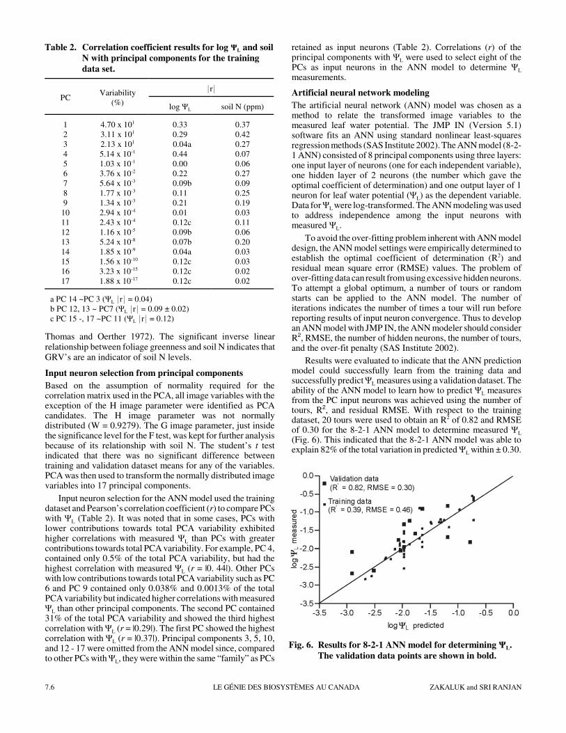
Results were evaluated to indicate that the ANN predictionmodel could successfully learn from the training data andsuccessfully predict ΨL measures using a validation dataset. Theability of the ANN model to learn how to predict ΨL measuresfrom the PC input neurons was achieved using the number oftours, R2, and residual RMSE. With respect to the trainingdataset, 20 tours were used to obtain an R2 of 0.82 and RMSEof 0.30 for the 8-2-1 ANN model to determine measured ΨL

(Fig. 6). This indicated that the 8-2-1 ANN model was able toexplain 82% of the total variation in predicted ΨL within ± 0.30.

Table 2. Correlation coefficient results for log ΨL and soil

N with principal components for the training

data set.

PCVariability

(%)

*r*

log ΨL soil N (ppm)

123456789

1011121314151617

4.70 x 101

3.11 x 101

2.13 x 101

5.14 x 10-1

1.03 x 10-1

3.76 x 10-2

5.64 x 10-3

1.77 x 10-3

1.34 x 10-3

2.94 x 10-4

2.43 x 10-4

1.16 x 10-5

5.24 x 10-8

1.85 x 10-9

1.56 x 10-10

3.23 x 10-15

1.88 x 10-17

0.330.29

0.04a0.440.000.22

0.09b0.110.210.01

0.12c 0.09b 0.07b 0.04a 0.12c 0.12c 0.12c

0.370.420.270.070.060.270.090.250.190.030.110.060.200.030.030.020.02

a PC 14 ~PC 3 (ΨL *r* = 0.04)b PC 12, 13 ~ PC7 (ΨL *r* = 0.09 ± 0.02)c PC 15 -, 17 ~PC 11 (ΨL *r* = 0.12)

Fig. 6. Results for 8-2-1 ANN model for determining ΨL.

The validation data points are shown in bold.


The R2 and RMSE for the validation dataset (0.39 and 0.46,respectively) suggested that the ANN model was an unreliablepredictor of ΨL at the plant level and was not unexpected.However, since irrigation occurs on a whole field basis, theANN model need only predict a whole field ΨL average(Zakaluk and Sri Ranjan 2007). As a result, validation data wereevaluated by comparing the mean and variance between thedistributions for predicted ΨL and measured ΨL (Table 3). Giventhat the variance and mean between the distributions were notsignificantly different and that the CV’s were similar, thepredicted ΨL and measured ΨL were shown to be from commonpopulations. Statistical evidence indicated that results can beused on well-watered potato plants, typically found in anirrigated field.

Since the t test indicated no significant difference betweenthe means of measured and predicted ΨL (Table 3), the strengthof the t test can be reviewed by calculating the smallestdifference the t test was likely to detect (least significant value).Based on the variances and sample size used in the validation ofthe ANN model, the smallest detectable difference for the t testwas 0.102 MPa and we can reasonably assume that both datasets were very similar.

Relative importance of input neurons

The responses of the eight principal components used as inputneurons were assessed to determine their RI for the ANN model(Table 4). Figure 7 illustrates the RI of each ANN model inputneuron. Figure 8 depicts a correlation curve for ΨL and soil Nfor each PC used in the ANN model ranked by relativeimportance. The fourth PC had the highest correlation with ΨL

(r = |0.44|) and the lowest correlation with soil N (r = |0.07|).Consequently the fourth PC had the highest relative importance(RI = 11.15%). The second PC had the second highest

correlation with ΨL (r = |0.29|). Although the second PC alsohad the strongest correlation with soil N (r = |0.42|), theseparation between ΨL and soil N made it the second highestinput neuron of relative importance (RI = 9.61%). Separationbetween correlations of ΨL and soil N with the eighth PC (r =|0.11| and r = |0.25|, respectively) made it the third highest inputneuron of relative importance (RI = 6.98%). The remaining PCs(11, 1, 9, 7, and 6) showed lower differences betweencorrelations with ΨL and soil N. In general, the PCs with moreseparation between ΨL and soil N correlations had more RI thanPCs with less separation between ΨL and soil N correlations.Based on the RI analysis, it appears that when there is lessseparation between ΨL and soil N, the RI decreases, suggestingthat soil N interacts with the determination of ΨL.

Table 3. Comparison of measured log ΨL and predicted log ΨL distributions for the validation dataset.

log ΨL n mean SD *CV*Shaprio - Wilk Bartlett’s Student’s t test

W p < W F ratio p > F t ratio p > *t*

measuredpredicted

1313

-1.75-1.90

0.570.63

3233

0.970.95

0.830.60

0.14 0.71 -1.00 0.34

Table 4. Relative importance of input neuron connection

weights with correlations against ΨL and soil N.

Inputneuron

RI(%)

*r*

log ΨL soil N (ppm)

PC 4PC 2PC 8

PC 11PC 1PC 9PC 7PC 6PC 3PC 5

PC 10

11.159.616.986.666.265.623.180.550.000.000.00

0.440.290.110.120.330.210.090.220.040.000.01

0.070.420.250.110.370.190.090.270.270.060.03

Fig. 7. Relative importance, in descending order, of each

input neuron across the ANN model.

Fig. 8. Correlation curves for ΨL and soil N against

relative importance (RI), in descending order, for

each input neuron used in the ANN model. PC 4,

PC 2, and PC 8 showed the most separation

between ΨL and soil nitrate and the highest RL.


Image parameter loadings of input neurons

Pearson’s correlation coefficient (r) was used to justify the eightPCs used as input neurons in the ANN model by comparingimage parameter loadings of the PCs, comparing the PCs withΨL, soil N, and radiometric calibration error (I) across images(Table 5). The highest loadings for the image parameters werefound in PC 1, PC 2, and PC 4. Although no strong relationshipcan be identified between the image parameters and PC 4 (r >|0.15|), the separation between soil N and ΨL indicated that PC 4was a separator between the two measured biophysical factors(Fig. 8). A comparison of the difference in correlations betweenthe PC 1 and PC 2 image parameter loadings suggested that red-blue and green-blue relationships were stronger in PC 1, whilegreen-red relationships were stronger in PC 2. In addition, PC 2contained the highest correlation with the green (G) image band(r = |0.70|), an indicator of soil N (r = |0.71|). The highercorrelation for I in PC 2 in comparison to PC 1 (r = |0.87| versusr = |0.06|) indicated that despite the higher correlation of PC 1with ΨL than PC 2 (Fig. 8), it can be concluded that soil N, asindicated by G, and radiometric calibration error as indicated byI, were the drivers for PC 2 that resulted in its higher relativeimportance in the ANN model.

Input neuron selection from the PCs required more than anexamination of their contribution towards total variability andimage parameter loading. For example, although PCs 6 – 9 andPC 11 lacked contributions towards total variability and lackedidentifiable image parameter loadings, they were neverthelessrequired in the ANN model due to their relationship with ΨL andsoil N (Fig. 8). For example, PC 8 contained low correlationswith all input image parameters, and yet due to the separation itprovided between ΨL and soil N (Fig. 8), it was the third mostimportant input neuron in the ANN model. PCs that containedlarge amounts of the total PC variability with readily apparentimage loadings was insufficient justification for their use. Forexample, PC 3 accounted for 29% of the total PC variability but

had a low correlation with ΨL (r = |0.04|) andredundant correlation with PC 6 and soil N r =|0.27|). In addition, previous research indicatedthat the third PC, derived from RGB imagebands, was related to soil clay content (Chen etal. 2004). Since soils, a biophysical parameter,were eliminated by image classification andPC 3 had a redundant correlation with PC 6,PC 3 was not required in the ANN model. ThePCs with no identifiable image parameterloadings or relationships with ΨL or soil N arelikely due to biophysical factors not measuredin this study such as: leaf age, leaf structure,and soil nutrients. Further study into otherbiophysical parameters with the PCs isrequired to account for their use in the ANNmodel. The PC omissions as input neuronsrequire analysis beyond image parameterloadings or contributions towards totalvariability.

Summary of findings

This research demonstrated the following:

1. The effects of shadow, soils, leafsenescence, and flowers could be isolatedfrom green leaf foliage using anunsupervised classification approach.

2. An inverse linear relationship was found between soil N andleaf reflectance in the green image band.

3. The measured ΨL and predicted ΨL validation datasets werefrom common populations and therefore ANN modelling ofΨL using RGB images shows promise as a tool fordetermining an average ΨL across a potato field forirrigation scheduling.

4. Input neurons with more separation between ΨL and soil Nwere more important in the prediction of ΨL, suggesting thatsoil N interacts with ΨL prediction when using RGB images.

5. The ground-based digital camera was able to supply RGBimages as an alternative to airborne-spaceborne imagingsensors.

These findings were similar to the results from an earliergreenhouse study (Zakaluk and Sri Ranjan 2007).

DISCUSSION

The results of this research may be explained in reference tovisible light and stomatal opening via guard cell chloroplasts.While guard cell chloroplasts are responsive to the red region(Olsen et al. 2002), guard cell chloroplasts are primarilystimulated by the blue region with the size of the stomatalopening following the level of visible light incident upon theleaf surface (Zeiger et al. 2002). Kleman and Fagerlund (1987)found that the Z chromaticity coordinate, a transformation of theblue spectral region, could be used to separate irrigated andunirrigated barley (Hordeum distichum L.) under fieldconditions. Schlemmer et al. (2005) found that compared to thered spectral region, corn (Zea mays L.) leaves had a closerinverse linear relationship with relative water content (RWC) inthe blue spectral region. Carter (1991) found that RWC wassensitive to the blue and red visible wavelengths centered at 480

Table 5. Pearson’s correlation coefficient (****r****) between image parameters

and the field ANN model input neurons (ranked by relative

importance).

Imageparameter

Input neuron

PC 4 PC 2 PC 8 PC 11 PC 1 PC 9 PC 7 PC 6

XYlog G/Blog BGGRS Xlog GBSlog RBSlog NDGBIIlog Slog RG/R XZlog R/BNDGRI Xlog NDRBI

0.150.130.030.000.040.030.050.050.030.010.010.050.120.010.040.140.03

0.400.730.410.730.700.260.270.470.420.870.320.920.730.280.100.730.10

0.000.000.000.000.000.000.010.000.000.010.010.010.000.000.000.000.00

4 x 10-5

6 x 10-4

3 x 10-5

4 x 10-4

4 x 10-3

3 x 10-4

1 x 10-3

4 x 10-4

9 x 10-4

4 x 10-3

4 x 10-4

2 x 10-4

1 x 10-3

5 x 10-4

3 x 10-4

1 x 10-3

6 x 10-4

0.730.520.910.590.250.020.800.880.910.06 0.830.320.240.960.970.240.97

0.000.000.000.000.010.000.000.000.010.000.000.000.000.000.000.000.00

0.010.010.000.000.010.000.010.010.000.010.020.000.000.000.000.000.02

0.010.000.030.020.020.010.020.020.020.030.020.010.000.010.030.000.02


and 680 nm for the leaves of six species. Given that the blue andred regions influence stomatal opening via guard cellchloroplasts and thus changes in ΨL due to water transpirationvia the stomata, the prediction of ΨL using PCA of R and Bcombinations is justified.

The green image band was an important contributor ofvisible light reflectance to the determination of ΨL. This studywas in agreement with previous studies (Schlemmer et al. 2005;Boegh et al. 2002; Osborne et al. 2002; Blackmer et al. 1994;Thomas and Oerther 1972) which showed that the green spectralregion had a linear association with N. While high soil N wasassociated with dark green color, low soil N was associated withleaf yellowing. Incorporating the green image band into thePCA contributed to the establishment of relationships betweenprincipal components, soil N, and ΨL, enabling the ANN modelto differentiate soil N from ΨL within the plant.

Monitoring chlorophyll absorption

While it might be argued that determining plant water stress inthe visible region via plant chlorophyll could be influenced byother plant physiological factors (Carter 1991; Ceccato et al.2001, 2002a, 2002b; Ripple 1986), strictly measuring plantwater content inside the SWIR region limits the possibility ofidentifying plant stress beyond plant water deficits. Forexample, there is no benefit to applying additional nitrogen overa low nitrogen area if the crop is under water stress (Christensenet al. 2005; Ebertseder et al. 2005). Ideally, for optimal cropproduction, a remotely-sensed imaging model should also bedeveloped to detect plant water stress and other plantphysiological factors.

This study indicated that a physiological change due tosoil N levels could be detected and isolated from the deter-mination of ΨL using visible light and an ANN model design.While future research using the protocol in this study may resultin agreement that visible leaf reflectance is not adequate forplant water stress detection, it may also be found that the onlychange, if any, may be in the ranking of the relative importancefor the input neuron weights in the determination of plant waterstress versus other plant physiological parameters. Moshou et al.(2003) used ANN modeling of five wavebands in the visible andNIR region to detect winter wheat (Triticum sp L.) stress underdifferent soil N levels and yellow rust (Puccinia striiformis f. sptritici) disease under field conditions. The use of ANNmodeling of remotely sensed images to monitor plant stressshows promise for the detection of plant water stress and plantdisease under different soil N levels. Based on findings fromthis study, further research is required to determine if other plantphysiological factors and other soil atmosphere factors could beisolated from the determination of ΨL using RGB images, anANN modeling approach, and relative importance analysis.

Sensor selection: Ground-based versus airborne-spaceborneimage acquisition

The results of this study may be attributed to the shortatmospheric transmission path (2.5 m), 0.91 mm spatialresolution data, and short timeline between image acquisitionand in situ ΨL measurement which may not be transferable tolower spatial resolution images acquired by aircraft or satellite.Satellite based images are susceptible to atmospheric error dueto the transmission path. In fact, wavebands on spaceborne

imaging sensors are selected to avoid atmospheric transmissionissues (Jensen 2005). While aircraft can design their imagingmissions to avoid atmospheric haze and clouds with moreflexibility than satellite imaging, satellite imaging relies on fixedrevisit rates that can only resolve haze and cloud cover issueswith the addition of more satellites. Images acquired withaircraft are also susceptible to hotspots caused by selecting thewrong combination of season and time of day for imageacquisition (Avery and Berlin 1992). Hotspots in the airborneimage create “whiteout” areas, which can make the imageimpossible to analyze.

According to Klotz et al. (2003), the use of a reference forreflectance values captured with a ground operated sensoreliminates the need for atmospheric correction models. Toevaluate the radiometric calibration technique used in this study,the coefficient of variation (CV) for intensity (I) wasdetermined. Intensity (I) is a measure of the mean for thedistribution of reflectance across an image that is not associatedwith any color and is hence an indicator of reflectance thatignores the RGB “colors” used in this research. As a result,radiometrically calibrated multi-temporal RGB images shouldhave similar intensities. The CV for intensity in this studyindicated that the radiometric calibration error across all imagesdid not exceed 4.99%.

Kostrzewski et al. (2002) reported that lower spatialresolutions smooth and reduce data variance, which supports theneed to choose an appropriate spatial resolution fitting for thestudy objectives. The use of aircraft or satellite images for thedetermination of ΨL would be a source of error in thedevelopment of the ANN model because of the lower spatialresolution and the time lag between image acquisition and insitu ΨL measures. In this study, a digital camera mounted on a2.5 m telescopic pole was used to eliminate the need foratmospheric correction through the use of standardizedreflectance reference and to optimize revisit rates to synchronizewith in situ measures of ΨL. If future research using airborne orspaceborne imaging sensors to determine ΨL is to follow theprotocol employed in this study, then the lower spatialresolution, limited revisit rates, and atmospheric correction willneed to be considered.

Experimental error associated with leaf water potential andsoil N

Results for the |CV| were 32% and 33% for both the measuredΨL and predicted ΨL datasets, respectively (Table 3). Accordingto Gomez and Gomez (1984), the CV is an indicator ofexperimental error and the acceptability of the CV depends onthe type of experiment. The CV for ΨL field data in researchconducted by Blad and Walter-Shea (1994) was between 62%and 85% for five grassland species collected over the KonzaPrairie in Kansas. In another field study of ΨL measurements onforest species (Almeida 2000), results indicated thatexperimental error for predawn ΨL measurements (CV = 47%)versus midday ΨL measurements (CV = 40%) was greater. Thisappears reasonable since during the midday period, sunlight isat a maximum, and stomatal resistance would be greater. Inaddition to the time of day for taking ΨL measurements, Naor etal. (2006) reported that variability in midday ΨL measurementscan be avoided by considering subfield variation caused byirrigation or soil hydraulic properties, sample storage, andhuman error of ΨL measurement.


In this study, ΨL measurements were taken from soil N plotsbetween the morning and late afternoon and thus contributed tothe experimental error. However, by ignoring soil N andrandomly selecting plots throughout the trial period, ΨL

measurements across plots were not biased by soil N. Forexample, if all low soil N plots were measured for ΨL during themorning, while all high soil N plots were measured for ΨL atmidday, there may have been some bias towards higher soil Nplots obtaining lower experimental error due to ΨL

measurement. To minimize experimental error, ΨL

measurements ideally should only be collected during themidday period. Based on Almeida (2000) and Blad and Walter-Shea (1994), the CV of ΨL measurements for this study werenevertheless within acceptable limits for this type of research.

CONCLUSION

This study examined RGB images, vegetation indices, andimage transformations derived from a ground based fivemegapixel RGB single CCD chip digital camera to determine ifΨL could be predicted for field potatoes. Existing soil N levelswere predetermined at each plot to account for soil N interactionwith measured ΨL.

Although the number of field samples was limited, a numberof conclusions was reached in this study. Using 0.91 mm spatialresolution images and under homogeneous plant conditions, theG and R image bands could be used to separate green foliagefrom shadow, soils, leaf senescence, and flowers. A significantinverse linear relationship between green foliage as measured bythe green image band and soil N was found (α # 0.05). Theground based five megapixel RGB digital camera providedcomparable distributions, means, and variances betweenmeasured ΨL and predicted ΨL using ANN modeling. PCAperformed on the RGB images and six image transformationsand nine vegetation indices found principal components withboth similar and different linear relationships with eithermeasured ΨL or measured soil N. The principal componentswith the greatest separation between measured ΨL and measuredsoil N were the most important input neurons for predicting ΨL

using ANN modeling of RGB images. The digital camera wasfound to be a viable option to airborne and spaceborne imagesacquisition methods.

Study findings may be attributable to the 0.91 mm spatialresolution images, the number of measurements used in thestudy, and/or the physiological relationships between the visiblelight reactions and water stress for potatoes. It remains unclearhow well the ANN modeling protocol will succeed across othercrops consisting of different canopy structures. Given theexploratory nature of this study, further research is required tovalidate the protocol and stability of input neuron RI beforeimplementation into a potato plant water stress monitoringprogram.

ACKNOWLEDGEMENTS

This research was financially supported in part by Red RiverCollege through a grant funded by Western EconomicDiversification Canada. The authors thank Frank Elias withKroeker Farms Limited for his invaluable assistance in makingthe potato field research possible.

REFERENCES

Almeida, D. 2000. LBA water potential data.http://ecophys.biology.utah.edu/public/LBA/Water_potential_data/ (2007/02/02).

Asrar, G., M. Fuchs, E.T. Kanemasu and J.L. Hatfield. 1984.Estimating absorbed photosynthetic radiation and leaf areaindex from spectral reflectance in wheat. Agronomy Journal

76: 300-306.

Avery, T.E. and G.L. Berlin. 1992. Fundamentals of remote

sensing and airphoto interpretation, 5th edition. UpperSaddle River, NJ: Prentice Hall.

Bastiaanssen, W.G.M. and M.G. Bos. 1999. Irrigationperformance indicators based on remotely sensed data: Areview of literature. Irrigation and Drainage Systems 13:291-311.

Blackmer, T.M., J.S. Schepers and G.E. Meyer. 1994. Remotesensing to detect nitrogen deficiency in corn. In Proceedings

of Site-Specific Management for Agricultural Systems, 505-512. Minneapolis, MN: ASA/CSSA/SSSA.

Blad, B.L. and E.A. Walter-Shea. 1994. Total Leaf TissueWater Potential (FIFE) Data set. http://www.daac.ornl.gov(2007/02/05).

Boegh, E., H. Soegaard, N. Broge, C.B. Hasager, N.O. Jensen,K. Schelde and A. Thomsen. 2002. Airborne multispectraldata for quantifying leaf area index, nitrogen concentration,and photosynthetic efficiency in agriculture. Remote Sensing

of Environment 81: 179-193.

Bowman, W.D. 1989. The relationship between leaf waterstatus, gas exchange, and spectral reflectance in cottonleaves. Remote Sensing of Environment 30: 249-255.

Carter, G. 1991. Primary and secondary effects of water contenton the spectral reflectance of leaves. America Journal of

Botany 78: 916-924.

Ceccato, P., S. Flasse, S. Tarantola, S. Jacquemound and J.M.Gregoire. 2001. Detecting vegetation leaf water contentusing reflectance in the optical domain. Remote Sensing of

Environment 77: 22-33.

Ceccato, P., N. Gobron, S. Flasse, B. Pinty and S. Tarantola.2002a. Designing a spectral index to estimate vegetationwater content from remote sensing data Part 1. TheoreticalApproach. Remote Sensing of Environment 82: 188-197.

Ceccato, P., S. Flasse and J.M. Gregoire. 2002b. Designing aspectral index to estimate vegetation water content fromremote sensing data Part 2. Validation and applications.Remote Sensing of Environment 82: 198-207.

Charles-Edwards, D.A., D. Doley and G.M. Rimmington. 1986.Modelling Plant Growth and Development. Orlando, FL:Academic Press.

Chen, F., D.E. Kissel, L.T. West and W. Adkins. 2004. Fieldscale mapping of surface clay concentration. Precision

Agriculture 5: 7-26.

Christensen, L.K., D. Rodriguez, R. Belford, V. Sadras, R.Rampart and P. Fisher. 2005. Temporal predictions ofnitrogen status in wheat under the influence of waterdeficiency using spectral and thermal information. InProceedings of the Fifth European Conference on Precision


Agriculture, 209-215. Uppsala, Sweden: Swedish Instituteof Agricultural and Environmental Engineering/SwedishUniversity of Agricultural Sciences.

Costa, L.D., G.D. Vedove, G. Gianquinto, R. Giovanardi and A.Peressotti. 1997. Yield, water use efficiency and nitrogenuptake in potato: Influence of drought stress. Potato

Research 40: 19-34.

del Moral, R. 1975. Vegetation clustering by means ofISODATA: Revision by multiple discriminate analysis.Plant Ecology 29: 179-190.

Eastman, J.R. and M. Fulk. 1993. Long sequence time seriesevaluation using standardized principal components.Photogrammetric Engineering & Remote Sensing 59: 991-996.

Ebertseder, Th., U. Schmidhalter, R. Gutser, U. Hege and S.Jungert. 2005. Evaluation of mapping and on-line nitrogenfertilizer application strategies in multi-year multi-locationstatic field trials for increasing nitrogen use efficiency ofcereals. In Proceedings of the Fifth European Conference

on Precision Agriculture, 327-335. Uppsala, Sweden:Swedish Institute of Agricultural and EnvironmentalEngineering/Swedish University of Agricultural Sciences.

Gamon, J.A. and J.S. Surfas. 1999. Assessing leaf pigmentcontent and activity with a reflectometer. New Phytologist

143: 105-117.

Gevrey, M., I. Dimopoulos and S. Lek. 2003. Review andcomparison of methods to study the contribution of variablesin artificial neural network models. Ecological Modelling

160: 249-264.

Gillespie, A.R., A.B. Kahle and R.E. Walker. 1987. Colorenhancement of highly correlated images. II. Channel ratioand "chromaticity" transformation techniques. Remote

Sensing of Environment 22: 343-365.

Gitelson, A., Y.J. Kaufman, R. Stark and D. Rundquist. 2002.Novel algorithms for remote estimation of vegetationfraction. Remote Sensing of the Environment 80: 76-87.

Gomez, K.A. and A.A. Gomez. 1984. Statistical Procedures for

Agricultural Research. New York, NY: John Wiley & Sons,Inc.

Gonzalez, R.C. and R.E. Woods. 2002 Digital Image

Processing, 2nd edition. Upper Saddle River, NJ: PrenticeHall.

Gunel, E. and T. Karadogan. 1998. Effect of irrigation appliedat different growth stages and length of irrigation period onquality characters of potato tubers. Potato Research 41: 9-19.

Haboudane, D., J.R. Miller, N. Tremblay, P.J. Zarco-Tejadaand L. Dextraze. 2002. Integrated narrow-band vegetationindices for prediction of chlorophyll content for applicationto precision agriculture. Remote Sensing of Environment 81:416-426.

Huete, A.R., D.F. Post and R.D. Jackson. 1984. Soil spectraleffects on 4-space vegetation discrimination. Remote

Sensing of Environment 15: 155-165.

Ingebritsen, S.E. and R.J.P. Lyon. 1985. Principal componentsof multitemporal image pairs. International Journal of

Remote Sensing 6: 687-696.

Jackson, T.J., D. Chen, M. Cosh, F. Li, M. Anderson, C.Walthall, P. Doriaswamy and E.R. Hunt. 2004. Vegetationwater content mapping using Landsat data derivednormalized difference water index for corn and soybeans.Remote Sensing of Environment 92: 475-482.

Jensen, J.R. 2005. Introductory Digital Image Processing, a

Remote Sensing Perspective, 3rd edition. Upper SaddleRiver, NJ: Prentice Hall.

Kanemasu, E.T. 1974. Seasonal canopy reflectance patterns ofwheat, sorghum, and soybean. Remote Sensing of


Karimi, Y., S.O. Prasher, H. McNairn, R.B. Bonnell, P.Dutilleul and P.K. Goel. 2005. Discriminant analysis ofhyperspectral data for assessing water and nitrogen stressesin corn. Transactions of the ASAE 48: 805-813.

Kleman, J.K. and E. Fagerlund. 1987. Influence of differentnitrogen and irrigation treatments on the spectral reflectanceof barley. Remote Sensing of Environment 21: 1-14.

Klotz, P., H. Bach and W. Mauser. 2003. GVIS groundoperated visible/near infrared imaging spectrometer. InProceedings of the Fourth European Conference on

Precision Agriculture, 315-323. Berlin, Germany: Centrefor Agricultural Landscape and Land Use Research/ Instituteof Agricultural Engineering Bornim.

Kostrzewski, M., P. Waller, P. Guertin, J. Haberland, P.Colaizzi, E. Barnes, T. Thompson, T. Clarke, E. Riley andC. Choi. 2002. Ground-based remote sensing of water andnitrogen stress. Transactions of the ASAE 46(1): 29-38.

McCoy, R.M. 2005. Field Methods in Remote Sensing. NewYork, NY: The Guilford Press.

McMurtrey, J.E., E.W. Chappelle, M.S. Kim, J.J. Meisinger andL.A. Corp. 1994. Distinguishing nitrogen fertilizer levels infield corn (Zea mays L.) with actively induced fluorescenceand passive reflectance measurements. Remote Sensing of


Moshou, D., C. Bravo, S. Wahlen, J. West and A. McCartney.2003. Simultaneous identification of plant stresses anddiseases in arable crops based on a proximal sensing systemand self organizing neural networks. In Proceedings of the

Fourth European Conference on Precision Agriculture,

425-431. Berlin, Germany: Centre for AgriculturalLandscape and Land Use Research/ Institute of AgriculturalEngineering Bornim.

Naor, A., Y. Gal and M. Peres. 2006. The inherent variabilityof water stress indicators in apple, nectarine, and pearorchards, and the validity of a leaf-selection procedure forwater potential measurements. Irrigation Science 24: 129-135.

Olsen, R.L., B.P. Pratt, P. Gump, A. Kemper and G. Tallman.2002. Red light activates a chloroplast-dependent ion uptakemechanism for stomatal opening under reduced CO2

concentrations in Vicia spp. New Phytologist 153: 497-508.

Osborne, S.L., J.S. Schepers, D.D. Francis and M.R.Schlemmer. 2002. Use of spectral radiance to estimate in-season biomass and grain yield in nitrogen- and waterstressed corn. Crop Science 42: 165-171.


Penuelas, J., J.A. Gamon, A.L. Fredeen, J. Merino and C.B.Field. 1994. Reflectance indices associated withphysiological changes in nitrogen- and water-limitedsunflower leaves. Remote Sensing of Environment 48: 135-146.

Ripple, W.J. 1986. Spectral reflectance relationships to leafwater stress. Photogrammetric Engineering and RemoteSensing 52: 1669-1675.

Rzempoluck, E.J. 1998. Neural Network Data Analysis UsingSimulnet™. New York, NY: Springer-Verlag.

SAS Institute. 2002. Jmp Version 5 Statistics and GraphicsGuide. Cary, NC: Statistical Analysis System, Inc.

Schlemmer, M.R., D.D. Francis, J.F. Shanahan and J.S.Schepers. 2005. Remotley measuring chlorophyll content incorn leaves with differing nitrogen levels and relative watercontent. Agronomy Journal 97: 106-112.

Scholander, P.F., H.T. Hammel, E.D. Bradstreet and E.A.Hemminsen. 1965. Sap pressure in vascular plants. Science148: 339-346.

Sony Corporation. 2004. ICX452AQF data sheet.http://www.eureca.de/pdf/optoelectronic/sony/ICX452AQF.PDF (2007/01/28).

Thomas, J.R. and G.F. Oerther. 1972. Estimating nitrogencontent of sweet pepper leaves by reflectance measurements.Agronomy Journal 64: 11-13.

Tremblay, N., H. Scharpf, U. Weier, H. Laurence and J. Owen.2001. Nitrogen Management in Field Vegetables - A guideto efficient fertilization. http://res2.agr.ca/stjean/publication/bulletin/nitrogen9-azote9_e.htm (2007/01/20).

Ustin, S.L. 2004. Manual of Remote Sensing, Volume 4, RemoteSensing for Natural Resource Management andEnvironmental Monitoring, 3rd edition. Hoboken, NJ: JohnWiley & Sons, Inc.

Waring, R.H. and B.D. Cleary. 1967. Plant moisture stress,evaluation by pressure bomb. Science 155: 1248-1254.

Wheeler, R.M. 2006. Potato and human exploration of space:Some observations from NASA-sponsored controlledenvironmental studies. Potato Research 49: 67-90.

White, A.M., G.P. Asner, R.R. Nemani, J.L Privette and S.W.Running. 2000. Measuring fractional cover and leaf areaindex in arid ecosystems: Digital camera, radiationtransmittance, and laser altimetry methods. Remote Sensingof Environment 74: 45-57.

Woebbecke, D.M., G.E. Meyer, K. Von Bargen and D.A.Mortensen. 1995. Color indices for weed identificationunder various soil residue and lighting conditions.Transactions of the ASAE 38: 259-269.

Zakaluk, R. and R. Sri Ranjan. 2007. Artificial neural networkmodelling of leaf water potential for potatoes using RGBdigital images–A greenhouse study. Potato Research 49:255-272.

Zeiger, E., L.D. Talbott, S. Frechilla, A. Srivastava and J. Zhu.2002. The guard cell chloroplast: A perspective for thetwenty-first century. New Phytologist 153: 415-424.

Zhurmar, A.Y. and E.A. Yanovskaya. 1992. Use of spectralinformation to estimate the mineral content of agriculturalcrops. Soviet Journal of Remote Sensing 10: 130-139.

LIST of SYMBOLS

AGL above ground level (m)ANN artificial neural networkB blue image band (8 bit)CCD charged couple deviceCV coefficient of variation (%)DAP days after plantingFC field capacity or upper soil water limit allowable

for plant growthG green image band (8 bit)GBS green blue slope (8 bit RV/nm)GB green blue simple ratio (dimensionless)GPS global positioning satelliteGR green red simple ratio (dimensionless)GRS green red slope (8 bit RV/nm)H hue transformation (8 bit)I intensity transformation (8 bit)N nitrate (ppm)NDGBI normalized difference green blue index

(dimensionless)NDGRI normalized difference green red index

(dimensionless)NDRBI normalized difference red blue index

(dimensionless)p probability levelPC principal componentPCA principal component analysisPWL peak wavelength (nm)R red image band (8 bit)r correlation coefficientR2 coefficient of determinationRB red blue simple ratio (dimensionless)RBS red blue slope (8 bit RV/nm)RMSE residual mean square errorRGB red green blue regions of the electromagnetic

spectrumRWC relative water content a soil (%)RI relative importance of input neuron (%)RV reflectance value response from an image (8 bit)TDR time domain reflectometry S saturation transformation (8 bit)SR simple ratio vegetation indexW Shapiro-Wilk test for normalityX chromaticity color coordinate transformationY chromaticity color coordinate transformationZ chromaticity color coordinate transformationα significance levelΨL leaf water potential (MPa)θV volumetric water content (%)

predicting the leaf water potential of potato plants using

Documents