predicting refrigerant inventory of hfc 134a in air cooled
TRANSCRIPT

Predicting Refrigerant Inventory of HFC 134a in Air Cooled Condensers
L. Orth, D. C. Zietlow, and C. O. Pedersen
ACRCTR-34
For additional information:
Air Conditioning and Refrigeration Center University of Illinois Mechanical & Industrial Engineering Dept. 1206 West Green Street Urbana, IL 61801
(217) 333-3115
April 1993
Prepared as part of ACRC Project 3 Condenser Peiformance
C. O. Pedersen, Principal Investigator

The Air Conditioning and Refrigeration Center was founded in 1988 with a grant from the estate of Richard W. Kritzer, the founder of Peerless of America Inc. A State of Illinois Technology Challenge Grant helped build the laboratory facilities. The ACRC receives continuing support from the Richard W. Kritzer Endowment and the National Science Foundation. Thefollowing organizations have also become sponsors of the Center.
Acustar Division of Chrysler Allied-Signal, Inc. Amana Refrigeration, Inc. Carrier Corporation Caterpillar, Inc. E. 1. du Pont de Nemours & Co. Electric Power Research Institute Ford Motor Company General Electric Company Harrison Division of GM ICI Americas, Inc. Johnson Controls, Inc. Modine Manufacturing Co. Peerless of America, Inc. Environmental Protection Agency U. S. Army CERL Whirlpool Corporation
For additional information:
Air Conditioning & Refrigeration Center Mechanical & Industrial Engineering Dept. University of Illinois 1206 West Green Street Urbana IL 61801
2173333115

Predicting Refrigerant Inventory of HFC 134a in Air Cooled Condensers
L. Orth, D.C. Zietlow, C.O. Pedersen
Department of Mechanical and Industrial Engineering
University of Illinois at Urbana-Champaign, 1993
ABSTRACT
Currently, the refrigerant inventory for vapor compression systems is determined using a costly trial and error procedure. An accurate computer model of the refrigerant in a system would reduce the time and expense of this process. This paper presents a computer model that has the capability to predict the amount of refrigerant in air cooled condensers.
For accurate prediction of refrigerant inventory two important steps are required. The first step is to model the heat transfer of the coil. This is needed to separate the three regions of the coil, de superheating, condensing, and sub cooling and then to further divide the condensing region into increments of quality.
The second step is to predict the void fraction (ratio of area occupied by gas to liquid) throughout the condensing region. Void fraction correlations by Domanski and Didion[ll], Hughmark[14], Premoli et al.[12], and Tandon et al. [10] are included in the model.
The simulation is used to model a cross flow heat exchanger, with parallel refrigerant paths, used in mobile air conditioning systems. The model is exercised to illustrate the effects of different operating conditions and void fraction correlations on the refrigerant inventory in condensers. A condenser used in mobile air conditioning applications is modeled. Future work includes experimental validation of the model.


TABLE OF CONTENTS
1.0 Introduction ......................................................................................................... 1
1.1 Nomenclature ..................................................................................................... 3
2.0 Simulation Description ..................................................................................... 6
2.1 Solution Technique ................................................................................ 6
2.2 Effectiveness-NTU Method .................................................................. 9
2.3 Air Side Heat Transfer Correlation ..................................................... 11
2.4 Refrigerant Side Heat Transfer Correlations ................................... 12
Single Phase Heat Transfer Correlation .......................................... 12
Two Phase Heat Transfer Correlations ........................................... 13
2.5 Refrigerant Pressure Drop Correlations ............................................. 14
Single Phase Pressure Drop Correlation ......................................... 15
Two Phase Pressure Drop Correlation ............................................ 16
2.6 Property Routines ................................................................................... 17
3.0 Coil Geometry and Modeling ........................................................................... 19
4.0 Prediction of Inventory ..................................................................................... 25
4.1 General Equations ................................................................................... 25
Single Phase Region ............................................................................ 26
Two Phase Region ............................................................................... 26
4.2 Void Fraction Correlations ................................................................... 28
Homogeneous ...................................................................................... 28
Domanski and Didion ........................................................................ 29
Tandon ................................................................................................... 29
Premoli. .................................................................................................. 30
Hughmark ............................................................................................. 30
4.3 Integral Solution Techniques .............................................................. .31
Closed Form .......................................................................................... 32
TABLE OF CONTENTS (continued)
Numerical Average ............................................................................. 32
4.4 Inventory Results ................................................................................... 33
Simulation Validation ...................................................................... .33
Solution Method .................................................................................. 35
Predicted Charge for Void Fraction Correlations ......................... .36
Inventory vs. Inlet Conditions ........................................................ .36
Inventory Distribution ...................................................................... .37
5.0 Future Work ........................................................................................................ 44
5.1 Overview .................................................................................................... 44
5.2 Schematics .................................................................................................. 44
5.3 Proposed Solutions to Weight Measurement Problems ................. .46
5.4 Test Plan ....................................................................................................... 47
6.0 References ............................................................................................................. 49
7.0 Appendix .............................................................................................................. 52

1.0 Introduction
Accurate prediction of the mass of a system component is important for
several reasons. In condenser modeling, accurate charge inventory prediction is
required for simulating off design performance and transient behavior. In system
modeling, the charge inventory of all components is required for the continuity
equation. This work focuses on predicting refrigerant inventory in air cooled tube
and fin condensers. In the single phase regions of the condenser, mass prediction is
a straight forward calculation. In the two-phase region, inventory is calculated
using a void fraction correlation. The void fraction correlation provides a ratio of
the tube cross sectional area occupied by refrigerant vapor to the total cross sectional
area for a given quality. There are many void fraction correlations available in the
literature; Domanski and Didion [11], Baroczy [18], Zivi [17], Smith [19], Premoli et al.
[12], Tandon et al. [10], and Hughmark [14]. The purpose of the work presented here
is to implement a number of these correlations into a condenser simulation
program to determine the mass of the condenser and provide a comparison of the
correlations for different operating conditions. Determination of the most accurate
correlation requires experimental data of the charge for the condenser coil being
modeled. This work will be available in the future and is discussed in section 5.0.
The condenser simulation program used for this study was originally
developed by Ragazzi [1]. The steady state simulation was designed to model air
cooled condensers which could be categorized as cross-flow heat exchangers with
circular refrigerant tubes with air flowing over them. It is based on first principles
and is general enough to use with condenser coils of various geometries and for
flows of different refrigerants. A complete description of the program and its
adaptation to various condenser coil geometries is provided. The various solution
techniques for the charge inventory correlations are also examined and compared.
1

The results indicate that the prediction of refrigerant inventory is influenced
by the selection of void fraction correlation and the predicted length of the
subcooling section in the condenser. This length is determined by the simulation
program and is dependent upon the correlations used for the refrigerant side heat
transfer coefficients and pressure drop. It will be shown that it is as important for
the condenser model to proper I y predict the outlet conditions as it is to predict the
overall capacity of the coil. Inventory comparisons are provided for the best
combination of heat transfer and pressure drop correlations.
In section 2 of the paper, an overview of the Module Based Condenser
Simulation program is provided. It outlines the solution technique and the
relevant heat transfer and pressure drop correlations. In addition, a discussion of
the thermodynamic property routines used in the simulation is provided. In
section 3, a description of the condenser coil used for this work is given. A
summary of the assumptions which were made is provided along with a detailed
description of how the coil was modeled. The void fraction correlations
implemented in the program are discussed in section 4, along with the integral
solution techniques and the final results. Future work to experimentally verify the
accuracy of the void fraction models is discussed in section 5.
2

1.1 Nomenclature
a Void fraction
A I Inside tube cross-sectionsl area ft2
Amean Mean tube cross-sectional area ft2
Asj(i) Module i inside surface area ft2
Aso(i) Module i outside surface area ft2
Cair(i) Module i air heat capacity rate Btu/hr-of
Cmax(i) Module i maximum heat capacity rate Btu/hr- of
Cmin(i) Module i minimum heat capacity rate Btu/hr- OF
cpMi) Module i air specific heat Btu/lbm-r
Cp air Condenser air specific heat Btu/lbm-r
cpf(i) Module i refrigerant liquid specific heat Btu/lbm-r
CpR (i) Module i refrigerant specific heat Btu/lbm-r
Cref(i) Module i refrigerant heat capacity rate Btu/hr- OF
Cratio(i) Module i heat capacity ratio
Di Inside tube diameter ft
Dh Air side hydraulic diameter ft
APcom Component refrigerant pressure drop psi
AP fric(i) Module i frictional refrigerant pressure drop psi
AP grav(i) Module i gravitational refrigerant pressure drop psi
AP mom(i) Module i momentum refrigerant pressure drop psi
AP mod(i) Module i total refrigerant pressure drop psi
C(i) Module i effectiveness
f Fanning friction factor
Fr Refrigerant Froude number
fQ (x) Heat flux assumption
G air Air side total mass flux Ibm/ft2-hr
G ref Refrigerant mass flux Ibm/ft2-hr
H Condenser height ft
hair Air side total heat transfer coefficient Btu/hr-ft2- OF
hair(i) Module i air side heat transfer coefficient Btu/hr-ft2- OF
h fg Latent heat of vaporization Btu/Ibm
href(i) Module i refrigerant side heat transfer coefficient Btu/hr-ft2- OF
h Rin ( i) Module i refrigerant inlet enthalpy Btu/Ibm
3

hRout(i) Module i refrigerant outlet enthalpy Btu/Ibm
j Colburn j-factor
k air Air thermal conductivity Btu/hr-ft- of
kf(i) Module i refrigerant liquid thermal conductivity Btu/hr-ft- of
kref(i) Module i refrigerant thermal conductivity Btu/hr-ft- of
k tube Tube thermal conductivity Btu/hr-ft- of
Leond Total refrigerant tube length ft
Lmod(i) Module i length ft
Lseg Segment length ft
mliq(i) Module i refrigerant liquid mass Ibm
mmod(i) Module i refrigerant mass Ibm
mtotai Total condenser mass Ibm
mvap(i) Module i refrigerant vapor mass Ibm
mA mod(i) Module i air mass flow rate lbm/hr
m Atot Total air mass flow rate lbm/hr
mRmod Module refrigerant mass flow rate lbm/hr
mRseg Segment refrigerant mass flow rate lbm/hr
mRtot Total refrigerant mass flow rate lbm/hr
n Number of modules in segment
1]s Air side overall efficiency
ntubes Number of tubes in manifold section
NTU Number of transfer units
NUair Air side Nusselt number
NUref(i) Module i refrigerant Nusselt number
«Pvap Two phase frictional multiplier
P Number of segments in condenser
Prair Air side Prandtl number
Prf(i) Module i refrigerant liquid Prandtl number
Prref(i) Module i refrigerant Prandtl number
PRin(i) Module i refrigerant inlet pressure psi
PRout(i) Module i refrigerant outlet pressure psi
Qmod(i) Module i total heat transfer Btu/hr
Reair Air side Reynolds number
Reeq(i) Module i equivalent Reynolds number
Ref (i) Module i liquid Reynolds number
Reg(i) Module i vapor Reynolds number
4

Reref(i) Module i refrigerant Reynolds number
Res(n,2) Residual equation array for n modules
Pavg(i) Module i refrigerant average density Ibm/ft3
Pf(i) Module i refrigerant liquid density Ibm/ft3
Pg(i) Module i refrigerant vapor density Ibm/ft3
Pref(i) Module i refrigerant density Ibm/ft3
(J Refrigerant surface tension
"wall Wall shear stress
TAin(i) Module i air inlet temperature of
T air in back Inlet air temperature to back modules of segment of
T avg out front Average air outlet temperature from front of
modules of segment
T Rin(i) Module i refrigerant inlet temperature of
VA Overall heat transfer coefficient
f.1air Air side viscosity lbm/ft-hr
f.1f(i) Module i refrigerant liquid viscosity lbm/ft-hr
f.1 g (i) Module i refrigerant vapor viscosity lbm/ft-hr
f.1ref (i) Module i refrigerant viscosity lbm/ft-hr
V(i) Module i refrigerant velocity ft/s
vf(i) Module i refrigerant liquid specific volume ft3/lbm
Vg(i) Module i refrigerant vapor specific volume ft3/lbm
Vin (i) Module i refrigerant inlet specific volume ft3/lbm
vout(i) Module i refrigerant outlet specific volume ft3/lbm
Wef Refrigerant liquid Weber number
Wg Heat flux averaged void fraction
xout(i) Module i refrigerant outlet quality
Xtt(i) Module i Lockhart-Martinelli correlating
parameter
5

2.0 Simulation Description
2.1 Solution Technique
The Module Based Condenser Simulation program is a general, first
principles condenser simulation which was developed to model air-cooled cross
flow condenser coils of various geometries. The general technique used by the
model is to divide the condenser coil into a user specified number of segments
which in turn are divided into a number of modules. The inlet conditions to the
segment are provided and then each module in the segment in treated as an
individual heat exchanger and a Newton-Raphson solution is performed to
determine the outlet conditions for each module. This procedure is used to analyze
all the segments in the condenser coil. The governing equations for each module
are the conservation of energy and momentum equations. These equations provide
a set non-linear equations which are then solved with a Newton-Raphson iteration
technique. A description of this technique is provided in Stoecker [2].
The operating conditions at the condenser coil inlet which must be specified
for the simulation are the refrigerant inlet pressure, temperature and mass flow rate
and the air inlet pressure, temperature, mass flow rate and relative humidity. These
are what will be referred to as the inlet test conditions. As stated earlier, each
module is treated as an individual heat exchanger so these same inlet variables
must be specified for each module. Certain assumptions are made to get this
information for each module, and hence, the accuracy of the solution is inherent on
the validity of these assumptions. For example, the condenser coil modeled by
Ragazzi consisted of two parallel, serpentine, finned tubes with air flowing normal
to the tubes. The inlet test conditions to the condenser coil were known (from
experiments). The coil was divided into two segments, the front tube and the back
tube. So the inlet test conditions on the refrigerant side for each segment were
assumed to be the same as those for the inlet to the condenser, with the exception of
6

the refrigerant mass flow rate which was assumed to be one-half of the total
refrigerant mass flow rate. This would also be the refrigerant mass flow rate for each
module.
[2.1]
For the air side inlet conditions, there is a slightly different situation. The
inlet air temperature and pressure for each module, in the first tube of the coil
modeled by Ragazzi, are equal to the inlet pressure and temperature for the test
point. The inlet air temperature to the second tube (segment) is set equal to the
average outlet air temperature from the first tube (segment). This is discussed in
greater detail in Ragazzi [1]. The air mass flow rate must also be determined. For
this example, it was assumed that the air flow rate in the duct was uniform so a
weighted average was taken to determine the mass flow rate over each module.
• _ • Lmod(i) mA mod(i) - mAtot x -
Lseg [2.2]
Here the weighting function is a ratio of the length of the module to the total length
of the segment, which is the total length of one tube. This weighting function
represents a ratio of the air flow area for the module to the total air flow area and
assumes that the refrigerant tubes are equally spaced. This weighting function can
change depending on the geometry of the coil. For example, if a condenser coil had
only one refrigerant tube, this tube could be modeled as any number of segments.
For this case, the total length of the condenser tube is used in the weighting function
instead of the length of one segment. The subscript (i) in equation [2.2] designates
the fact that this value will (or may) change for each module and will be utilized
throughout this paper. This subscript is not used for the refrigerant module mass
flow rate because this value is constant throughout a segment.
One additional determination needs to be made for the condenser
simulation, and that is whether the user wants to fix the length of a module or the
7

outlet quality of the module. The example above would work well with either of
these versions. The module length could be specified for each module and the
program will solve for the outlet quality. If the outlet quality is specified for each
module then the program determines the length of each module required to obtain
this condition. Both versions have their advantages and disadvantages. For
example, the fixed quality version is useful if the length of each of the condenser
regions (superheated vapor, two phase and subcooled liquid) is to be determined.
For more complicated geometry, however, the fixed length version is more
adaptable to the coil geometry as will be shown later. One source of error in the
fixed length version is a result of the determination of the local refrigerant side heat
transfer coefficients. The heat transfer correlation used for a module is always based
on the outlet conditions. For example, if the inlet condition of a module is
superheated vapor and the outlet condition of the module is two phase, then the
program uses the two phase correlation to determine the heat transfer coefficient for
the entire module. In reality, the transition from superheated vapor to two phase
occurred somewhere in the module. This problem would only occur at the two
transition points (superheated vapor to two phase refrigerant, and two phase
refrigerant to subcooled liquid), and can be compensated for somewhat by making
the length of the modules smaller.
As stated previously, the simulation uses a Newton-Raphson solution
technique for each segment to determine the outlet conditions of each module. The
Newton-Raphson variables for both versions of the simulation are the module
outlet enthalpy (hRout(i) and the module outlet pressure (PRout(i)' The residuals
equations for the Newton-Raphson iteration are given by,
R (. 1) h h Qmod(i) h h Qmod(i) es l, = Rout(i) - Rin(i) -. = Rout(i) - Rout(i-l) - • mRmod mRmod
[2.3]
Res(i, 2) = PRout(i) - PRin(i) - L1Pmod(i) = PRout(i) - PRout(i-l) - L1Pmod (i) [2.4]
8

In equation [2.3], Qmod(i) represents the total heat transfer from the module and in
equation [2.4] tJ.Pmod(i) represents the total pressure drop in the module. The total
heat transfer is calculated using an effectiveness-NTU method and the total pressure
drop is calculated using a pressure drop correlation.
For certain coil geometries, an additional Newton Raphson variable is used.
This variable is the average outlet air temperature from the from the modules. This
situation occurs when the refrigerant tube is wrapped from the front of the coil to
the back of the coil with a return bend and the refrigerant inlet to the tube is located
in the back. In this situation, the portion of the tube at the back of the condenser
requires the average air oulet temperature from the portion of the tube in the front
of the coil to use as its inlet air condition. This is accomplished by modeling the
tube as one segment and having an equal number of modules in both the front and
rear portions of the tube. The Newton-Raphson residual equation which is added to
the iteration is given by,
Res = T air in back - T avg out front [2.5]
A more in depth discussion of this procedure is provided in Zietlow [24].
2.2 Effectiveness-NTU Method
The effectiveness-NTU method is used in the condenser simulation to
determine the heat rejected by each module (Qmod(i). The general form of the
equation is,
[2.6]
The module effectiveness C(i) is defined as the ratio of the actual heat transfer rate to
the "ideal" or maximum heat transfer rate. This value is dependent on the ratio of
heat capacity rates and the number of transfer units (NTU).
C Cmin(i) ratio(i) = C
max(i)
9
[27]

NTU=~ Cmin(i)
[2.8]
The heat capacity rates are calculated for the both the refrigerant and the air and the
minimum value of these is Cmin(i) and the maximum value is designated as Cmax(i)'
The heat capacity rate is the mass flow rate times the specific heat.
Cair(i) = rnA mod(i) X CpA(i)
[2.9]
[2.10]
The variable VA in equation [2.8] is the overall heat transfer coefficient and is the
sum of the convective resistances on the air side and refrigerant side of the
condenser coil along with the conductive resistance of the tube wall.
UA = ---=1-----1-:---------:;-1-- [2.11] ----- + + ----
The effectiveness is then calculated for one of three cases:
1. Cmin(i) = Cair(i) and the refrigerant is single phase
- 1 [_ -[ 1-e-NTU ]xCratio(i) 1 C(i) - 1 e
Cratio(i) [2.12]
2. Cmin(i) = Cref(i) and the refrigerant is single phase
[ -NTUxC to (0)] - 1-e ra 10' /Cratio(i) C(i) = e [2.13]
3. Refrigerant is two phase:
1 -NTU C(i) = - e [2.14]
The third case is the limiting case which occurs in the condensing region when the
refrigerant side specific heat approaches infinity. Once the coil geometry and
material are specified, equation [2.11] indicates that there are three unknowns in the
equation which must be determined: 1]s' hair(i) and href(i). The formulation for
determining these variables will be provided in the next sections.
10

2.3 Air Side Heat Transfer Correlation
The air side heat transfer coefficient (haiT(i) used in the simulation program
for the charge inventory analysis is the Colburn j-factor. The j-factor is determined
for the condenser coil using experimental data and a modified Wilson plot
technique [3]. The modified Wilson plot is used to provide the surface efficiency (11s)
of the coil in addition to the j-factor correlation. If no experimental data are
available, Kays and London [13] have tabulated data for various heat exchanger
geometries which can be used to determine this correlation. The general
formulation for the j-factor is:
where,
. NUaiT ) = 1/3
ReaiT PraiT
h· Dh Nu· = Air Nusselt Number = _a_IT_ alT kair
G ·Dh ReaiT = Air Reynolds Number = _a,,_
J.lair
. I J.laiTCp aiT Prair = AIr Prandt Number = ---'--
kair
[2.15]
[2.16]
[2.17]
[2.18]
Once the j-factor has been determined for various data points using the modified
Wilson plot technique, a correlation for the j-factor can be found as a function of the
air side Reynolds number. A least squares fit was utilized in the determination of
this correlation. For the coil used in this paper, this correlation was found to be,
j = O. 166 Reair -0.4 [2.19]
The heat transfer correlation is then found by rearranging equation [2.15] and
canceling terms.
h. = GaiT CpaiT j azr P 2/3
raiT [2.20]
11
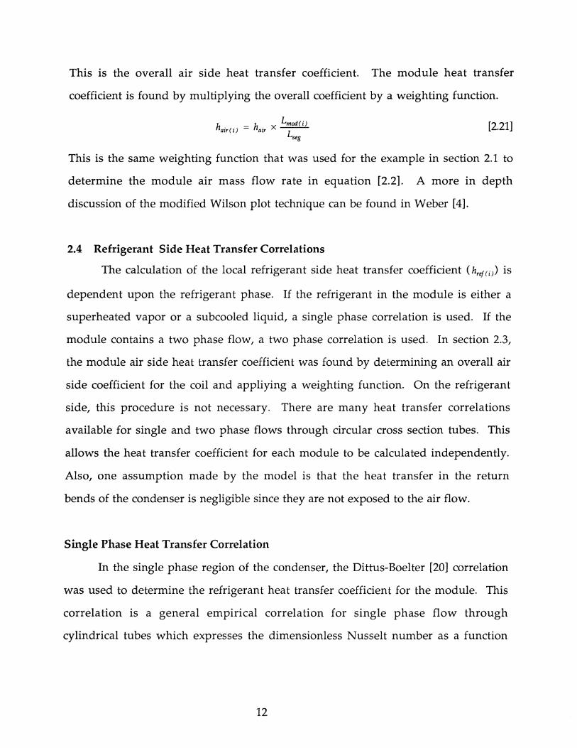
This is the overall air side heat transfer coefficient. The module heat transfer
coefficient is found by multiplying the overall coefficient by a weighting function.
h h Lmod(i) air(i)::= air X --
Lseg [2.21]
This is the same weighting function that was used for the example in section 2.1 to
determine the module air mass flow rate in equation [2.2]. A more in depth
discussion of the modified Wilson plot technique can be found in Weber [4].
2.4 Refrigerant Side Heat Transfer Correlations
The calculation of the local refrigerant side heat transfer coefficient (href(i) is
dependent upon the refrigerant phase. If the refrigerant in the module is either a
superheated vapor or a subcooled liquid, a single phase correlation is used. If the
module contains a two phase flow, a two phase correlation is used. In section 2.3,
the module air side heat transfer coefficient was found by determining an overall air
side coefficient for the coil and appliying a weighting function. On the refrigerant
side, this procedure is not necessary. There are many heat transfer correlations
available for single and two phase flows through circular cross section tubes. This
allows the heat transfer coefficient for each module to be calculated independently.
Also, one assumption made by the model is that the heat transfer in the return
bends of the condenser is negligible since they are not exposed to the air flow.
Single Phase Heat Transfer Correlation
In the single phase region of the condenser, the Dittus-Boelter [20] correlation
was used to determine the refrigerant heat transfer coefficient for the module. This
correlation is a general empirical correlation for single phase flow through
cylindrical tubes which expresses the dimensionless Nusselt number as a function
12

of the dimensionless Reynolds and Prandtl numbers. The general form of this
correlation for cooling is given by,
NUref(;) = 0.023 x Reref (i)°.8 x Prref (i)°.3 [2.22]
The heat transfer coefficient for the module is related to the Nusselt number by,
[2.23]
The dimensionless Reynolds number and Prandtl number for the module are given
by, R mR mod X D;
eref(i) = A; x J.lref(;)
[2.24]
P _ J.lret(;) X CpR(i) rret(i) - k
rete;)
[2.25]
It should be noted that additional single phase correlations are available for
use in the simulation program and can be found in Ragazzi [1].
Two Phase Heat Transfer Correlations
In the calculation of condenser mass inventory, two refrigerant two phase
correlations will be compared, the Cavallini-Zecchin [5] and Dobson [6]. Both
correlations were developed for annular flow regimes. The Cavallini-Zecchin
correlation is one of the most general empirical correlations. It was developed using
a large amount of data from various substances. The Dobson correlation, on the
other hand, was developed specifically for R134a. Overall it was found that using
the Dobson correlation provided more accurate results for the condenser outlet
conditions. This will be discussed in greater detail in the results section.
The general form of the Cavallini-Zecchin correlation is given by,
h 0.8 0.33 [ kt(i) ] ref(;) = 0.05 x Reeq(;) x Prr(;) D; [2.26]
13

where,
[ ][ ]0.5
Jig(i) Pf(i) Reeq(i) = Ref(i) + Reg(i) -- --
Jif(i) Pg(i)
[2.27]
[2.28]
eref x Di ( ) Reg(i) = Xout(i)
Jig(i)
[2.29]
[2.30]
The Dobson correlation which was developed for R134a is a function of the
Lockhart-Martinelli correlating parameter Xu. Its general form is given by,
[2.31]
where,
[ ]0.5 []0.125 0.875
Xtt(i) = Pg(i) Jif(i) [ 1 - Xout(i) ]
Pf(i) Jig(i) Xout(i)
[2.32]
and hf(i) is the liquid heat transfer correlation,
[2.33]
Equation [2.33], is the Dittus Boelter single phase liquid heat transfer given by
equation [2.20], and the liquid Reynolds number and Prandtl number have the same
definition as given by equations [2.28] and [2.30].
2.5 Refrigerant Pressure Drop Correlations
As was the case for the refrigerant heat transfer coefficient, the refrigerant
pressure drop across the module is dependent on the phase of the refrigerant. The
simulation program contains both single phase and two phase pressure drop
correlations. In addition to this, there are three components for the module
14
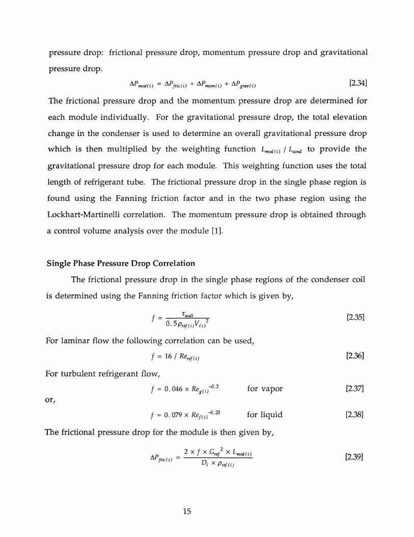
pressure drop: frictional pressure drop, momentum pressure drop and gravitational
pressure drop.
[2.34]
The frictional pressure drop and the momentum pressure drop are determined for
each module individually. For the gravitational pressure drop, the total elevation
change in the condenser is used to determine an overall gravitational pressure drop
which is then multiplied by the weighting function Lmod(i) / Lcond to provide the
gravitational pressure drop for each module. This weighting function uses the total
length of refrigerant tube. The frictional pressure drop in the single phase region is
found using the Fanning friction factor and in the two phase region using the
Lockhart-Martinelli correlation. The momentum pressure drop is obtained through
a control volume analysis over the module [1].
Single Phase Pressure Drop Correlation
The frictional pressure drop in the single phase regions of the condenser coil
is determined using the Fanning friction factor which is given by,
For laminar flow the following correlation can be used,
f = 16 / Reref(i)
For turbulent refrigerant flow,
f = 0.046 x Reg (i)-O·2 for vapor or,
f = 0.079 x Ref(i)-O·25 for liquid
The frictional pressure drop for the module is then given by,
2 x f x Cre/ x Lmod(i) !!..P fric(i) = -----'-----'
Di X Pref(i)
15
[2.35]
[2.36]
[2.37]
[2.38]
[2.39]

The momentum pressure drop for the module is given by,
[2.40]
The gravitational pressure drop for the module is given by,
flP H[ Lmod(i)] grav(i) = Pref(i)gc -L--cond
[2.41]
Two Phase Pressure Drop Correlation
A separated flow model was used in the simulation to calculate the pressure
drop in the two phase region. It was developed by Lockhart and Martinelli based on
their studies of air-water flows. The general form of the two phase pressure drop
correlation is given by,
_ 2[ 2 x ivap x Gre/ x XOl<t(i/ x Lmod(i) ] flP fric(i) - <l>vap D. x P .
I ge,) [2.42]
where <l> is a two phase frictional multiplier which is dependent on whether there is
laminar or turbulent flow in the liquid and vapor, and ivap is the vapor Fanning
friction factor given by equation [2.37]. Various forms for <I> are available in the
literature, Soliman et al. [15] and Chisholm [16]. The two-phase frictional multiplier
developed by Soliman et al. was for the case of both turbulent liquid and vapor (the
turbulent-turbulent case) and is given by,
85 X 0.523 <l>vap = 1 + 2. tt(i) [2.43]
where XI/(i) is the Lockhart-Martinelli parameter given by equation [2.32]. The
momentum pressure drop is found by applying a momentum balance to the
module which yields,
flP (.) = -G e/{[~ + (1- xf] _ [~+ (1- X)2]} [2.44] mom I r Pga Pi (1 - a) out(i) Pga Pi {1 - a) in(i)
16

where a is the void fraction correlation proposed by Zivi [17] and is given by,
1 [2.45] a=------.......,..-;-;;-1 + [~][Pg(i) ]2/3
X Pfeil
The gravitational pressure drop is calculated based on a homogeneous flow
model and has the same general form as the single phase pressure drop except an
average density is used.
LlP H[ Lmod(i) ] grav(i) = Pavg(i)gc -L--cand
[2.46]
where,
Pavg(i) = [ 1 1 Vf(i) + Xli) ( Vg(i) - Vf(i))
[2.47]
2.6 Property Routines
The thermodynamic property subroutines utilized by the simulation were
developed by the National Institute of Standards and Technology (NIST) [7]. The
use of these subroutines allows for greater flexibility in the model. There is a choice
of two equations of state, the Benedict-Webb-Rubin (BWR) or the Carnahan
Starling-DeSantis (CSD) equation of state. In addition, there are coefficients for the
CSD equation of state for up to 26 refrigerants and mixtures of up to five
components can be analyzed. The BWR subroutines are more accurate, especially
for R134a which is the reference refrigerant [8]. When using the Benedict-Webb
Rubin equation of state, properties for other refrigerants are found using the
principle of corresponding states. The CSD equation of state subroutines were
chosen for use in the simulation program because they allowed the flexibility of
looking at mixtures.
A comparison of the enthalpy change and saturation temperatures for the
two equations of state for R134a was made to determine the error that could result
through the use of the less accurate CSD equation of state. It was found that there
17

were errors in the saturation temperatures of less than 0.5 %. For the latent heat, it
was found that the error in the CSD equation of state (EOS) ranged from 3.4% to
4.7% for a saturation pressure of 150 psi to 250 psi which is shown in Figure 2.1.
The experimental data taken for the condenser coil is also analyzed with the
CSD equation of state subroutines, so this error should not affect the validation of
the simulation. An interface program was written for use with the FORTRAN
subroutines. This interface allows the subroutines to be implemented into existing
programs with relatively few problems.
Comparison of Hfg for R134a Figure 2.1
80,-------------------------------~
75~------------------------------_1
~ 70 ........ .a 65 e eo
:E 60
55
50
Saturation Pressure [psi]
18
II CSD EOS ~ BWR EOS

3.0 Coil Geometry and Modeling
The condenser coil used for the inventory analysis is a cross-flow tube and fin
heat exchanger with a fairly complex geometry. This section provides an overview
of the coil geometry along with a discussion of the assumptions made in the
computer modeling and the changes to the simulation required to include the
manifold and return bend pressure drop.
The inlet to the condenser coil is a manifold which is divided into a number
of sections where the refrigerant flows in and out of the refrigerant tubes. In each of
these sections, a number of tubes circulate the refrigerant through the width of the
condenser and return to the manifold where the refrigerant drops into the next
section of tubes. Figure 3.1 below, is a top view of the condenser coil which shows
the manifold inlet and the top tube configuration.
Figure 3.1 - Condenser Top View
4arufoldWet/ / / / / / / / Refrigerant Tube
Air How Air How I Drawing not to scale I
Figure 3.2 on the next page, shows the number sections in the condenser coil
and the number of refrigerant tubes in each section. It also indicates the air flow
direction and whether the refrigerant inlet is in the front of the tube or the rear of
tube. This is an important point in the condenser modeling. In section 2.1, it was
shown that the modeling of a refrigerant tube whose air inlet was in the front and
refrigerant inlet was in the rear required the additional Newton-Raphson variable
19

which determined the average air outlet temperature from the front of the
refrigerant tube to use as the air inlet temperature to the back of the refrigerant tube.
This will greatly affect the number of segments required to model this coil.
Section 1 Set of 4 tubes
Rear Tube Inlet
Section 2 Set of 4 tubes
Front Tube Inlet
Section 3 Set of 3 tubes
Rear Tube Inlet
Section 4 Set of 3 tubes
Front Tube Inlet
Section 5 Set of 3 tubes
Rear Tube Inlet
Section 6 Set of 3 tubes
Front Tube Inlet
Section 7 Set of 2 tubes
Rear Tube Inlet
Figure 3.2 - Condenser Front View
Air Flow Air Flow
///////// .. ................ ......... ... . ........................... ... .......... . ....... . ....... . ... .
..... .,. .. ... ..... ........ . ..................... .,; ................... .
••••••••• ',' ....................... ".jo" ••••••••••••••••• ;. •••••••••••••••• ;.=- .•.•... ";W'O ••••• ;. ....... .
.. x ....
: .... •.•. !'
. .. . .. " ... .......... ..... . .......... " ........ .
..... ........ .... ............ ...... ..,., .. .............. ................. ... ... ...... .; ... .-
.... ... .. ....... ...... ..... .... .... . ........................................ '" ....... .
Manifold Drawing not to scale I
20
Return Bends Not Shown
Rear Tubes Not Shown

It should be noted that the distance between manifold sections in figure 3.2
has been exaggerated to enhance the clarity of the figure. This type of geometry
requires the use of the fixed length version of the simulation program, because it is
not possible to specify before hand the inlet and outlet quality of the segments.
These values will be determined by the simulation. For this coil geometry, the
condenser coil is divided into ten segments. The manifold sections which have a
rear inlet are modeled as one segment (sections 1, 3, 5 and 7), alternatively, the
sections with a front inlet are modeled as two segments (sections 2, 4 and 6).
As stated previously the coil is modeled by ten segments. It is assumed that
the inlet conditions to all of the tubes in each manifold section are equivalent. This
allows the use of only one tube in the Newton-Raphson solution. Table 4.1 below
shows the number of modules each segment was divided into for the inventory
results presented in section 4.4.
Table 3.1 Number of Modules per Segment for Inventory Analysis
Manifold Section Segment Number Number of Modules 1 1 10 2 2 5
3 5 3 4 10 4 5 5
6 5 5 7 10 6 8 5
9 5 7 10 10
Table 4.2 gives some of the overall condenser dimension needed to run the
simulation.
21

Table 3.2 - Condenser Dimensions
Variable Value Units
Condenser Total Tube Length 81.4 ft
Condenser Frontal Tube Length 40.7 ft
Inside Tube Diameter 0.204 in
Outside Tube Diameter 0.235 in
Here the total condenser tube length is used in the weighting function to determine
the gravitational pressure drop in the module given by equations [2.41] and [2.46].
The frontal condenser tube length is used to determine the air flow rate over a
module given by equation [2.2] and the air side heat transfer coefficient in equation
[2.21]. The frontal length is used because this represents the ratio of the area which
the module air flow occupies to the total air flow area assuming the refrigerant tubes
are equally spaced.
Certain assumptions are made to determine the refrigerant properties along
the condenser length. The first assumption made is that refrigerant mass flow rate
entering the tubes from the manifold is uniformly divided among the number of
tubes giving, . mRtot
mRmod = -ntubes
[3.1]
In addition, the inlet conditions to each tube in the manifold section are assumed to
be equal (the inlet pressure, temperature and enthalpy). The return bends and
manifold are assumed to be adiabatic since they are not exposed to the airflow.
However, the pressure drop accross the bends and manifold were included in the
sim ula tion.
For example, the inlet pressure and temperature to the condenser is specified
by the user. The program determines the condenser inlet enthalpy and the pressure
22

drop in the first manifold. So the inlet conditions to the first segment are the
enthalpy at the inlet of the condenser and the inlet pressure minus the manifold
pressure drop. With these two thermodynamic properties set, all the additional
segment inlet conditions are found using the thermodynamic property routines.
The simulation then solves the Newton-Raphson problem for the first segment
which provides the outlet conditions of the first segment. To determine the inlet
conditions for the second segment, the inlet enthalpy is equal to the outlet enthalpy
of the first segment (the manifold is adiabatic). The inlet pressure is the outlet
pressure of the first segment minus the manifold pressure drop. Return bend
pressure drops are calculated only in manifold sections which are modeled with two
segments.
This procedure continues until all segments of the condenser have been
analyzed. The total mass of the condenser is then given by,
[3.2]
If there were only one refrigerant tube per segment then the total mass of the
condenser is given by,
n
mtotal = I. mmod(i)
i=l
[3.3]
The pressure dop correlations for the manifolds and return bends were
developed by Paliwoda [23]. He developed a generalized method for determining
the pressure drop across pipe components with two-phase flow. This includes,
manifolds, return bends, T-junctions, valves, etc. The general component pressure
drop correlation for the condenser is given by,
Cr/ X ~ X f3e L1P = ----"~---
eom 2xp x g ge
[3.4]
23

For this condenser's manifold,
~ = 2.7 [3.5]
and,
Pc = [8 + O. 58x{1 - 8)][1 - x ]0.333 + x2.276 [3.6]
where,
[ jO.25
8 = Pg J.li Pi J.lg
[3.7]
For the return bends,
~ = 0.12 [3.8]
and,
Pc = [8 + 3.0x{1- 8)][1- x]0.333 + x2.276 [3.9]
Overall it was found that the frictional pressure drop in the return bends was
on the same magnitude as was found for the frictional pressure drop in straight
modules. The manifold frictional pressure drop on the other hand was quite large
in comparison to the pressure drop in straight modules. The next section of the
paper discusses the void fraction correlations and the charge inventory equations
used to find the mass of the modules.
24

4.0 Prediction of Inventory
The simulation program solves for the outlet conditions for each module, the
temperature, pressure, quality, enthalpy, etc. It is these values which are needed to
determine the refrigerant mass in each module using a void fraction correlation.
Five different correlations were added to the simulation for comparison purposes.
These are the homogeneous void fraction model [21], the Domanski and Didion
correlation [11], the Tandon et al. correlation [10], the Premoli et al. correlation [12]
and the Hughmark correlation [14]. Section 4.1 presents an overview of the general
governing equations needed to calculate the refrigerant inventory. In section 4.2 the
specific format for each of the void fraction models is presented. The different
solution techniques are discussed in section 4.3 and results are presented in section
4.4.
4.1 General Equations
The general refrigerant inventory equations are provided for both the single
phase region and two phase regions of the condenser. In the single phase region,
the condenser mass is a function of the density and volume of the module only. In
the two phase region, the mass is also a function of the quality which leads to a
more complicated integral equation as will be shown. The mass of each module is
determined using its inlet and outlet conditions, and then the total condenser mass
is found by taking the summation of all the module masses.
n
mtotal = L mmod (i)
i=l
[4.0]
The general void fraction equations are available in the literature and Rice [9]
provides an excellent summary of these equations.
25

Single Phase Region
In the single phase region of the condenser, the refrigerant mass is a function
of the density and module volume.
[4.1]
where L = 4nod(i)' Since the cross sectional area of the condenser is constant (the tube
inside diameter is constant), this equation can be integrated and the result is:
mmod(i) = V mod(i) X Pavg(i) = Ai X Lmod(i) x Pavg(i) [4.2]
For better accuracy, the average density across the module is used.
Two Phase Region
In the two phase region of the condenser, the total mass of the module can be
found by adding the mass of the liquid and the mass of the vapor together.
mmod(i) = mvap(i) + mliq(i) [4.3]
To determine the mass of the vapor and liquid in the module the same integral that
was used in equation [4.1] is performed for the vapor and liquid refrigerant
separately. The mass of the vapor present in the module is given by,
[4.4]
and the mass of the liquid present in the module is given by,
[4.5]
The void fraction alpha is defined as the ratio of the cross sectional area occupied by
the vapor to the total tube cross sectional area, a = Ag / Ai' Equations [4.4] and [4.5]
can then be written in the following form,
mvap(i) = P g Ai r a . dl [4.6]
and,
26

mliq(i) = Pt Ai foL (1 - a) . dl [4.7]
The total refrigerant mass in the module is then given by,
mmod(i) = Ai[Pg foL a . dl + Pt foL (1 - a)· dl] [4.8]
The void fraction is generally a function of quality so it is desired to transform
the integral over the length of the module to an integral over the quality of the
module. In order to do this, an assumption regarding the heat flow must be made
to determine the relationship between the quality and the tube length [9]. The mass
integral equation [4.8] is then normalized with this function and integrated over the
quality. The total heat transferred from a module can be represented by the
following equation,
[4.9]
Recognizing that the refrigerant mass flow rate and the latent heat of vaporization
are constants, the integral in equation [4.6] for the mass of the vapor can be
normalized and the result is a heat flux averaged void fraction wg •
[4.10]
Equation [4.8] then becomes,
[4.11]
Now the calculation of the module mass is dependent on evaluating the integral in
equation [4.10]. In order to do this, as stated earlier, an assumption regarding the
heat flux along the length of the tube must be made. The simplest assumption
which can be made is that the heat flux is constant, in which case, it drops out of the
integral leaving, lXOUf(i) a dx
W - _.....:Xin~(.!.!.i) __ _ g(i) -
Xout(i) - Xin(i) [4.12]
27

This assumption is dependent on their being a linear relationship between
the quality and tube length. The design of the simulation program is well suited for
this assumption if a large number of modules is used. If a large number of modules
is used, the change in quality along the length of the module will be small and could
therefore, be approximated by a linear distribution without much error. This will be
investigated in more detail in the results section. The next section outlines the void
fraction models which will be used in this study.
4.2 Void Fraction Correlations
The void fraction correlations available in the literature were reviewed by
Rice [9] who categorized them into four groups:
1. Homogeneous 2. Slip ratio correlated 3. Xtt correlated 4. Mass flux dependent
The Domanski-Didion correlation can be categorized as Xtt correlated while the
Premoli and Hughmark correlations are categorized as mass flux dependent. The
Tandon correlation is both Xtt correlated and mass flux dependent. No slip ratio
correlated void fraction models were used in the simulation program.
Homogeneous
The homogeneous void fraction is the most simplistic form available. It is a
function of the quality and the vapor-liquid density ratio. The general form of the
equation is given by [21], 1 [4.13] a = --------
l+[l-XJPg
x Pf
This void fraction model along with the constant heat flux assumption can be
integrated over the quality change of the module to obtain a closed form solution
for the homogeneous void fraction. This solution will be provided in section 4.3.
28

Domanski and Didion
The Domanski and Didion [11] void fraction correlation is based on the
Lockhart-Martinelli correlating parameter Xtt and the data available from the
pressure drop work of Lockhart-Martinelli [22]. It was developed by Domanski and
Didion for use in a heat pump simulation. The general formulation is,
[ 0.8 ]-0.378 a = 1 + Xtt for Xtt ::; 10 [4.14]
and,
a = O. 823 - O. 157 In Xtt for Xtt > 10 [4.15]
where,
[4.16]
Tandon
The Tandon et. al. [10] void fraction equation includes both the effects of
frictional pressure drop and mass flux by correlating as a function of the liquid
Reynolds number and the Lockhart-Martinelli correlating parameter. The void
fraction equations are,
a- 1 f + f [ 1. 928 Re -0.315 0.9293 Re -0.63]
- - F(Xtt ) F(XttP for 50 < Ref < 1125 [4.17]
or,
a- 1 f + f [ 0.38 Re -0.088 0.0361 Re -0.176]
- - F( Xtt ) F ( Xtt P for Ref ~ 1125 [4.18]
where,
[4.19]
and
[4.20]
29

Premoli
The Premoli et al. [12] correlation is a function of the liquid Reynolds
number, Weber number and the surface tension. It is given by,
where, -0.19 [ ]0.22 F1 = 1. 578 Ref Pt!Pg
-0.51 ( )-0.08 F2 = 0.0273 Wef Ref Pt!Pg
y = _/3_ 1-/3
1 /3 = --::----::---1 + [1 -x] Pg
x Pf
[4.21]
[4.22]
[4.23]
[4.24]
[4.25]
[4.26]
[4.27]
Here we start to see that the integrals to evaluate Wg can get quite complicated as
the void fraction models become more complex. It is not clear if a closed form
solution even exists for these integral equations, therefore, numerical methods of
evaluating the integrals is discussed in section 4.3.
Hughmark
The Hughmark void fraction correlation is one the most complex and
requires an iterative solution. The correlation is given by,
[4.28]
30

where KH is a function of the correlating parameter Z. These values are tabulated in
Table 4.1. The correlating parameter Z is given by,
Table 4.1
Re 1/6 Fr1.8 [4.29] Z= a
YL1.4
Hughmark Flow Parameter Data Z KH
where, 1.3 0.185
Rea = Dj Gre! [4.30]
J.i.! + a(J.i.g - J.i.! )
1.5 0.225 2.0 0.325 3.0 0.490
1 [G~ xl [4.31] Fr = gc Dj /3 Pg
4.0 0.605 5.0 0.675 6.0 0.720 8.0 0.767
YL = 1 - /3 [4.32] 10.0 0.780 15.0 0.808
/3= 1 [4.33]
1 + [1 - x] Pg
x Pg
20.0 0.830 40.0 0.880 70.0 0.930 130.0 0.980
These are the five void fraction correlations which were added to the
condenser simulation program and will used for the comparison of predicted
condenser charge. The next section reviews the solution techniques used to
evaluate the integral W g.
4.3 Integral Sol ulion Techniques
The calculation of the refrigerant mass in each module of the condenser is
dependent on evaluating the integral equation for W g for each void fraction model.
Two solution techniques were explored, a closed form expression and a numerical
average of the inlet and outlet void fraction values. A closed form expression for
the homogeneous void fraction correlation was found. This is useful in verifying
the results obtained for the numerical average approximation. For the other void
31

fraction correlations, the numerical average is performed. This section describes the
procedure and assumptions used for these solution techniques.
Closed Form
The closed form expression is the exact solution for the heat flux averaged
void fraction for the module. As the void fraction correlations increase in
complexity, however, this expression is more difficult to find if it exists at all. For
the homogeneous model, the integration was performed to obtain the following
expression,
[4.34]
where,
and, [4.35]
This closed form solution will be utilized to determine the accuracy of the
numerical average technique.
Numerical Average
The numerical average technique consisted of taking a numerical average of
alpha at the inlet and outlet of the module. The assumption made here is that there
is a linear quality distribution along the module length. This is the same
assumption which was made for the use of the constant heat flux assumption in the
formulation of W g in section 4.1 and similar reasoning applies here. For a small
module length, relative to the total length of the condenser, the change in quality
from the inlet to the outlet is small and W g can be approximated by an average of
the inlet and outlet void fraction. Clearly, the accuracy of this technique is
dependent on this assumption being satisfied. If the entire two phase region of the
32

condenser is being modeled with one module, one might need to investigate
additional numerical integration techniques.
4.4 Inventory Results
Simulation Validation
In section 2, a discussion of the two phase refrigerant heat transfer
correlations indicated that there were some differences between the Cavallini
Zecchin and the Dobson correlations for both the prediction of the overall coil
capacity and the total pressure drop. This is the first comparison provided. In
Figure 4.1, a comparison of the total heat transfer is provided for the two
correlations. The comparison is against the experimental heat transfer found for the
same operating inlet conditions. Overall, the average magnitude of error for the
Cavallini-Zecchin correlation was 6.33% while the Dobson correlation was 8.62%.
The Cavallini correlation overpredicted the heat transfer in most cases while the
Dobson correlation underpredicted the heat transfer. In general, the Cavallini
correlation better predicted the heat transfer for this coil. The pressure drop results
are shown in Figure 4.2. The average magnitude of error using the Cavallini two
phase heat transfer correlation was 33.11 %, while for the Dobson correlation it was
21.38%. The underprediction of heat transfer from the Dobson correlation results in
a longer two phase region in which a higher pressure drop exists. This increases the
overall pressure drop predicted by the simulation. The heat transfer correlations
also have a significant implact on the length of the subcooling region. The
Cavallini correlation overpredicted the heat transfer which resulted in a long
subcooling region. The Cavallini correlation predicted an average of 14.35 of
subcooling while the Dobson correlation predicted no sub cooling with an average
outlet quality of 0.0898. The experimental data indicated an average of 1.5 of
subcooling. The Dobson correlation decreases the sub cooling length and therefore
33

provides a better inventory prediction. Figure 4.3 shows a comparison of the charge
prediction for the two correlations using the homogeneous close form void fraction.
50
'til 0.. 0:. 40 0
0 (I) 30 ... ;:l VJ VJ (I) ...
0... 20 r:: ,9 (U
10 "S S
U)
0
Heat Transfer Comparison Figure 4.1
50~--------------------------------~~--
O~~--~------~----~----~~----~ o
0
10 20 30
Experimental Q [Btu/Ibm) Thousands
40
Pressure Drop Comparison Figure 4.2
Experimental Pressure Drop [psi)
34
50
o Dobson <> Cavallini
o Dobson <> Cavallini
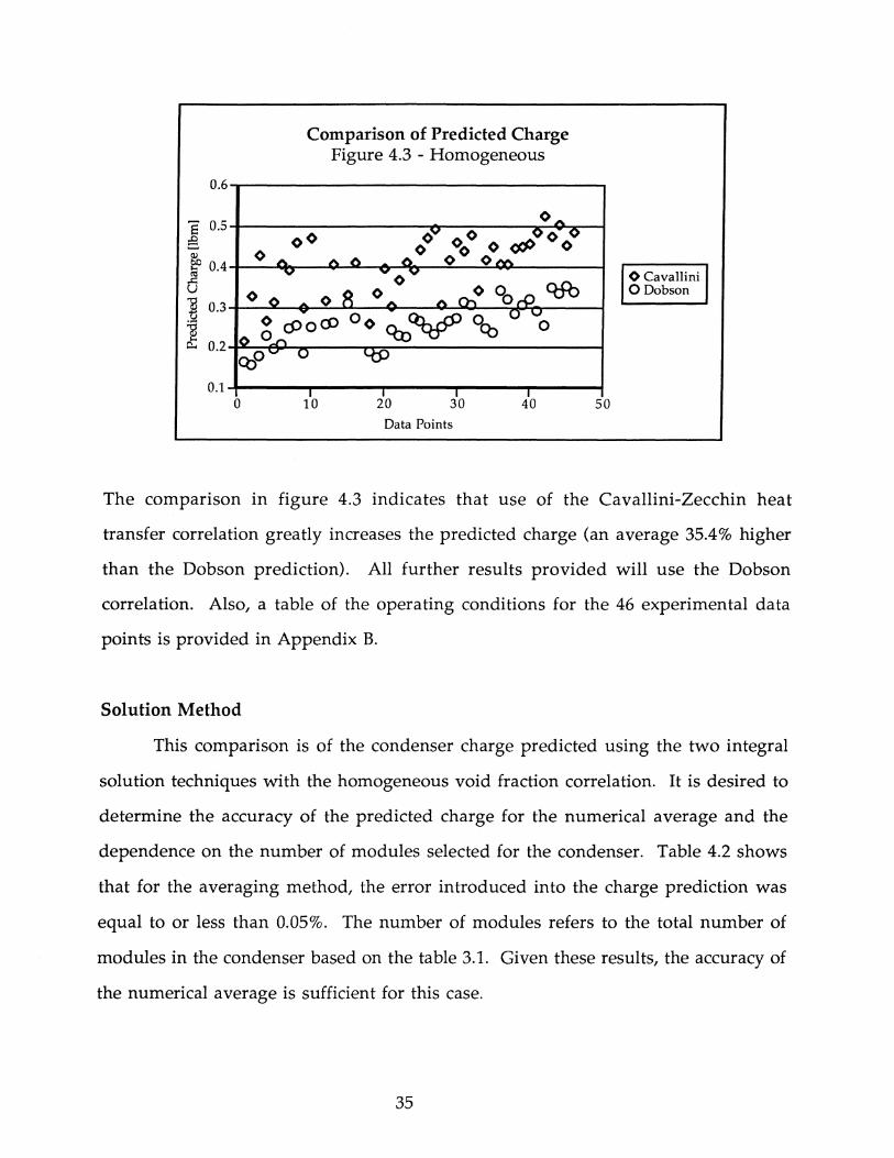
Comparison of Predicted Charge Figure 4.3 - Homogeneous
0.6 __ ------------------.
0.1-+----,...--..,..---.,....--....,.----1 o 10 20 30 40 50
Data Points
o Cavallini o Dobson
The comparison in figure 4.3 indicates that use of the Cavallini-Zecchin heat
transfer correlation greatly increases the predicted charge (an average 35.4% higher
than the Dobson prediction). All further results provided will use the Dobson
correlation. Also, a table of the operating conditions for the 46 experimental data
points is provided in Appendix B.
Solution Method
This comparison is of the condenser charge predicted using the two integral
solution techniques with the homogeneous void fraction correlation. It is desired to
determine the accuracy of the predicted charge for the numerical average and the
dependence on the number of modules selected for the condenser. Table 4.2 shows
that for the averaging method, the error introduced into the charge prediction was
equal to or less than 0.05%. The number of modules refers to the total number of
modules in the condenser based on the table 3.1. Given these results, the accuracy of
the numerical average is sufficient for this case.
35

Table 4.2 - Error for Numerical Average
Number of Modules Percent Error - Average
70 0.020
48 0.033
24 0.050
Predicted Charge for Void Fraction Correlations
Figure 4.4 shows the predicted condenser charge for the different void fraction
correlations. Overall, it is seen that the Hughmark correlations consistantly predicts
the greatest charge, the next highest predictor is the Premoli correlation, and the
Tandon, Domanski and homogeneous correlations seem to be in the same general
area.
Predicted Charge For Void Fraction Models Figure 4.4
0.5-.---------------------,
0.45-1---------------:------,1
& 0.4
~ 0 .35 -f-~~r_d:~:_bh_Cii~~.,......._=i::IR_T"T""__'=I__l=:::l
o 0.3 ~I....,;,...--,I
~ 0.25 ~~IIiP~~---, ] ~ 0.2~-............. .__--_=_------------,I
0.15-t=-------------------,I
0.1 -1----...... ---.,...---,.----,------4 o 10 20 30 40 50
Data Ponts
Inventory vs. Inlet Conditions
• Homogeneous • Domanski • Tandon o Premoli <> Hughmark
A comparison of the predicted charge versus various conditions is made. The
charge was compared with the overall heat transfer and pressure drop. In addition,
36

it was compared with the inlet pressure, refrigerant mass flow, and air mass flow
rate. The most significant dependence of the predicted charge is on the inlet
refrigerant pressure. This dependence is shown in figure 4.5 below.
Predicted Charge vs. Inlet Pressure Figure 4.5
0.5....--------------------,
0.45 -f-----------------::;;::----i
~ 0.4-t---9----:~:__ll~~~~~~~1:JI2m1 We 0.35 +--~J::I-~>*:~Ii""I""~~_'f"i_"'I""Fri;;_.....,fiitlll-l ~ u 0.3 -r--..,..,r::-~t::iiiMr-'tra ..... -~
~ 0.25 +----==" ...... ~ ... ~ 0.2-1---~~1_I1I_:::__-----------1
0.15-1---l1li--='---------------1
0.1-+----..,...---..,...---..,..----1 1
Condenser Inlet Pressure [psi]
Inventory Distribution
II Homogeneous • Domanski • Tandon [J Premoli <> Hughmark
This last section of results provides a comparison of the mass distribution
along the condenser length for the module vapor, liquid and total module mass.
This comparison is based on the results for a single tube. For example, for this coil
geometry, the first manifold section contained four tubes. Only the mass of the
modules in one of these tubes will be compared. This will provide a clearer picture
of what effect the quality distribution has on the predicted module charge and also
what effect the refrigerant mass flux has on the module charge. There are two mass
flux transitions within this coil. The first occurs between the second and third
manifold sections where the number of refrigerant tubes is reduced from four to
three. The second transition occurs between the sixth and seventh manifold
37

sections where the number of refrigerant tubes is reduced from three to two. It is
desired to see what effect, if any, these transitions will have.
The comparison was made for three data points at different air mass flow
rates. These points were selected for their low outlet qualities which allowed most
of the condensing region to be modeled. The data points used were six, ten and forty
from the Appendix. Figure 4.6 below shows the distribution for point six which had
the highest air mass flow rate of the three. The Hughmark correlation predicts a
larger module mass throughout the condensing section. It is also interesting to
note, the mass flux transition points had no noticeable effect on the module mass.
12
10
S ::9
~ 8
(/)
a .r::. '6
Q) c :3 CIS 6 (/)
~ :::J 0
.r::.
"S I-
.~ 4 "'C
J: 2
0 0
Predicted Module Mass Distribution Figure 4.6 - Air Mass How Rate: 6509.8 [Ibm/hr]
~
~IZ!I ~~r:'I AAoO
~ ijO ~~A
XX~O&O xxxXi i 6& 0
xxxxxg8i g DO XXX BaBBS 000000 x 88
.S~~DD 000000
5 10 15 20 25
Condenser Length [ft)
30
Mass Flux Transition
o Homogeneous o Domanski A Tandon o Premoli X Hughmark
Figure 4.7 shows the module mass distribution for point ten. In this diagram
the predicted refrigerant mass increased much more sharply towards the end of the
condensing region than it did in Figure 4.6. This is due in part to the low refrigerant
38

mass flow rate in combination with the high air flow rate which provides a faster
condensing rate.
Predicted Module Mass Distribution Figure 4.7 - Air Mass Flow Rate: 4092.6 Dbm/hr]
0.02 _._----...,.....-----------:-------,
~ 0.Q15
~ a f3 0.01
~ al .tl "0 J: 0.005
o 5 10 15 20 25 30
Condenser Length [ft]
Mass Flux Transition
o Homogeneous <> Domanski ll. Tandon o Premoli X Hughmark
Figure 4.8, is the module mass distribution for point forty. The predicted
module mass for these operating conditions shows a much more gradual increase
along the length of the condenser. The refrigerant mass flow rate for this case was
about the same as for point 10 while the air mass flow is about half. The first few
modules in the figures represent the superheated region of the condenser where the
mass is found without the void fraction correlation and so it is the same for all the
curves. Figure 4.9, shows the liquid mass distribution along the length of the
condenser coil for point six. It is found that the liquid distribution curves are almost
the same as the module mass distribution curves. This is due to the dominating
effect the liquid has the total module mass.
39

12
10
S @ ~ 8
a (/) .s:::. .:0
..sl c: a1 6 ::s (/)
"0 ::l 0 0
::E .s:::.
~ I-
4
£ 2
0
10
9
S 8 @
~ 7 ..c:: U (/) "0 .s:::. 6 ·S .:0 0'" c: .... a1
5 ....l (/)
~ ::l 0
-g .s:::. 4 I-::E "0 3 .21 .S=! "0 2 J:
1
0
0
0
••
Predicted Module Mass Distribution Figure 4.8 - Air Mass Flow Rate: 2197.1 [lbm/hr1
XX X
.I~~
5 10 15 20 25 Condenser Length [ft]
Predicted Module Liquid Mass Distribution Figure 4.9 - Air Mass Flow Rate: 6509.8 [Ibm/hr1
5 10 15 20 25
Condenser Length [ft]
40
30
30
Mass Flux Transition
o Homogeneous <> Domanski b. Tandon o Premoli X Hughmark
Mass Flux Transition
o Homogeneous <> Domanski b. Tandon o Premoli X Hughmark
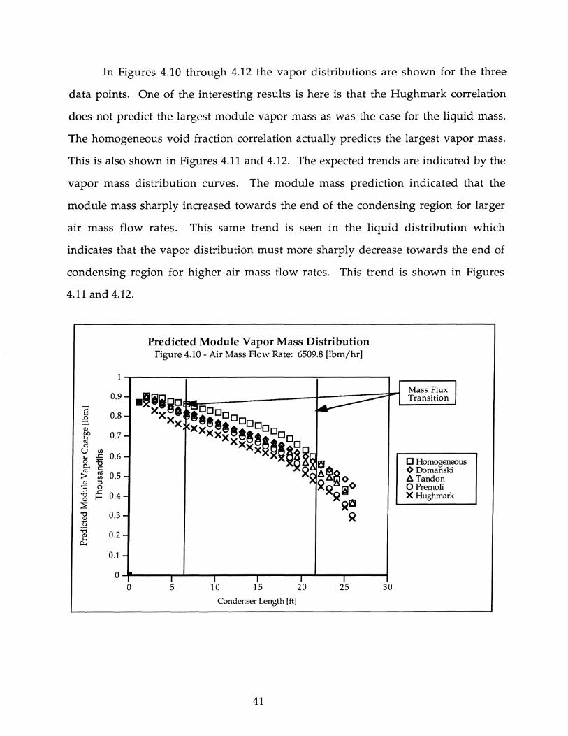
In Figures 4.10 through 4.12 the vapor distributions are shown for the three
data points. One of the interesting results is here is that the Hughmark correlation
does not predict the largest module vapor mass as was the case for the liquid mass.
The homogeneous void fraction correlation actually predicts the largest vapor mass.
This is also shown in Figures 4.11 and 4.12. The expected trends are indicated by the
vapor mass distribution curves. The module mass prediction indicated that the
module mass sharply increased towards the end of the condensing region for larger
air mass flow rates. This same trend is seen in the liquid distribution which
indicates that the vapor distribution must more sharply decrease towards the end of
condensing region for higher air mass flow rates. This trend is shown in Figures
4.11 and 4.12.
1
0.9
S 0.8 @ w co 0.7 ... <!l ..c:: u CJ)
0.6 ... .c o -0.."0 <II c:
:> ffi 0.5 -&
:::J 0 .c "'0 I- 0.4 0 ::;s
"8 0.3 t)
] 0.2 ... 0..
0.1
0 0
Predicted Module Vapor Mass Distribution Figure 4.10 - Air Mass Flow Rate: 6509.8 [lbm/hr]
.~ii~D Xx 0 80000 Xx 088 DOD xXxx88eeDDDD
Xx ee~ 0 xxxxx~e~~
~ Q ~~~O Q~ IilO
~~ra ~
5 10 15 20 25
Condenser Length [ft]
41
30
Mass Flux Transition
o Homogeneous <> Domanski ~ Tandon o Premoli X Hughmark

s ~ ~ a U) ... .r:; o -p.,"O m c: :> ~ J:! :;, ::s 0
"0 .r:; 0 I-~ "0
QJ
.~ ] p.,
S @
QJ
fa e U) ... .r:;
o -p.,"O m c: :> ~
QJ :;,
"S 0 "0
.r:; 0 l-~ 13 tl :a J:
0.8
0.7
0.6 • 0.5
0.4
0.3
0.2
0.1
0 0
Predicted Module Vapor Mass Distribution Figure 4.11 - Air Mass Flow Rate: 4092.6 [lbm/hr]
.~iii 00000
3333S0000o XXX xxxxx3gggg%
Xx ~<>o XXx ~<>e
~t.1!J ~t. ~
5 10 15 20 25 Condenser Length [ft]
Predicted Module Vapor Mass Distribution Figure 4.12 - Air Mass Flow Rate: 2197.1 Ubm/hr]
30
2.5 -.-------:..----------~----___.
2 ii~ ~~~iii~ ·X
• Xx 1.5 xxx~OOo!l!1I1!1l98 • XXX 00 <><>
XXXOO ~A XXO
X~Q 1 X
0.5
O~----~~----~----~------~~--~----~ o 5 10 15 20 25 30
Condenser Length [ft]
42
Mass F1ux Transition
o Homogeneous <> Domanski t. Tandon o Premoli X Hughmarl<
Mass F1ux Transition
o Homogeneous <> Domanski t. Tandon o Premoli X Hughmark

Overall, these results reinforce the belief that the accurate prediction of the
condenser mass is based upon the accurate prediction of the condenser liquid mass.
In order to determine the most accurate void fraction correlation for this purpose it
is necessary to measure the condenser mass. This work will be available in the
future and is discussed in the next section.
43

5.0 Future Work
5.1 Overview
The future work consists of an experiment which measures the weight of the
refrigerant in a condenser during operation. The experimental measurement will be
compared with the simulation results to determine which void fraction correlation
produces the best results. The condenser to be tested is different than the one
discussed in this paper. It consists of micro channel tubes with headers at the inlet
and outlet of the tubes. It will be modeled using the same techniques described in
this paper.
5.2 Schematics
The following schematic illustrates the instrumentation and components used in
the experimental apparatus for condensers. The apparatus has the capability to
control the fluid flow rates and inlet conditions. The pre and after condensers
provide the capability for partial condensing. A refrigerant turbulator is used at the
entrance to the test section to promote thermodynamic equilibrium between the
liquid and the vapor.
44

Condenser Apparatus
~ U1
Air In
Air blender
Filter
Air Out
Subcooling Control
i
t:::::)
Schrader Valve
Supply Fan w/ Speed Controller
C?
Low Range Pump
Hot/Chilled Water Coil
iTlTIl 1111111 111111 !I!IV
.v-Receiver
Filter/Drier
Instrumentation legend
High Range Pump
D-differential pressure, F-f1ow, H-humidlty, P-pressure, T-temperature ,W-weight
(r)(p) Airflow Measurement Station w/ Nozzles
Air Loop
......--tD\---w Refrigerant Turbulator
--Refrigerant Loop
Equipment legend
C><3 Shut-off valve or Schrader valve
ty
8i Manual expansion valve WN Capillary tube
~ Sight glass rzza Air filter ~ Air blender
Air blender
Heater/Superheater

The details of the weight measurement system are given in the following figure.
cable
load cell
pivot point
air flow ......
counterweight
oil bath
Layout of Test Section - side view
5.3 Proposed Solutions to Weight Measurement Problems
BeIth and Tree [25] describe a design to accurately measure the weight of refrigerant
in each of the components of a heat pump. On the following page is a list of
problems they encountered, along with the current design's proposed solutions to
these problems.
Weight measurement problem Proposed solution
Component weight greater than Use a balance beam with a co un ter
refrigerant mass weight
Refrigerant movement causes false Suspend the condenser from above
readings when using a balance with a using a cable
single pivot point
46

Drag and lift forces cause errors in With no refrigerant flow the lift
the mass measurement forces will be measured for different
air flow rates
The stiffness of the piping and duct Flexible ducting made of 5 mil plastic
connections affect the vertical will be used between the coil and the
movement of the component fixed duct. Flexible refrigerant hose
will be used to connect the
component to the rest of the loop.
Rigid mounting of the cantilever Mount the transducer so there can be
beam transducers limited the movement between the transducer
deflection of the balance beam and the balance beam
Friction or dam ping from the pivot Make all pivot points knife edges
points, when bearings were used,
caused a hysteresis loop the same
magnitude as the expected output
The balance beam vibrated Immerse the counter weight into an
oil bath to dampen the vibrations.
5.4 Test Plan
Before testing can begin, the weight measurement system will be calibrated. This
calibration will account for two different effects. The first is the effect of the flexible
connections on the mass measurement. This will be accounted for by placing a series
of known masses, covering the range of expected refrigerant mass, on top of the
empty test section and recording the output of load cell. Then the offset and span
can be determined from a curve fit of this data.
The second effect is the lift force caused by air flow over the coil. This will be
accounted for by recording the output of the load cell at different air flow rates that
cover the entire operating range of the condenser. The output of the load cell will be
corrected in an analysis program using the relationships developed during the
calibration.
The test plan may consist of two phases. In phase one the refrigerant will enter the
test section at or near saturated vapor conditions, and exit the test section at or near
saturated liquid conditions. In other words, complete condensation will occur
47

during the testing. After the first phase the data will be analyzed to determine if
partial condensing data are needed. Many of the void fraction correlations were
developed for a particular flow regime (e.g. Tandon-annular flow) and may not be
able to be applied over the full condensing region. If this is the case then the
different flow regimes may need to be studied separately.
Since it is not possible to observe the flow regimes in the tubes of the condenser,
some criteria will be needed to determine where the flow regime changes. Tests of a
compact heat exchanger (Dh=1.74 mm) by Damianides and Westwater [26] does
provide a starting point. They tested water air mixtures at 5.4 atmospheres. The
superficicial liquid velocity varied from 0.0838 to 8.62, and the superficial gas
velocity was from 1.05 to 101.2 m/s. They observed that smooth stratified and wavy
stratified flow regimes were absent. Comparing the test envelop with their flow map
suggests that there will be two flow regimes: intermittent and annular. If phase two
testing is necessary, a dimensional analysis will be conducted to check the validity of
the Damianides flow map for this application.
The exit header introduces a significant amount of uncertainty (-35%) in the weight
measurement. For this reason some method of flow visualization will be
implemented to qualitatively access the amount of liquid in the exit header. With
the flow visualization technique we hope to reduce this uncertainty to within 10%.
48

6.0 References
[1] Ragazzi, F., "Modular-Based Computer Simulation of an Air-Cooled Condenser", M.S. Thesis, University of Illinois at Urbana-Champaign, 1991.
[2] Stoecker, W.F., Design of Thermal Systems, 3rd ed., McGraw-Hill Publishing Co., New York, 1989, p125.
[3] Stoecker, W.F., and J.W. Jones, Refrigeration and Air Conditioning, 2nd ed., McGraw-Hill Publishing Co., New York, 1982, p236.
[4] Weber, R.J., "Development of an Experimental Facility to Evaluate the Performance of Air-Cooled Automotive and Household Refrigerator Condensers Utilizing Ozone-Safe Refrigerant", M.S. Thesis, University of Illinois at Urbana-Champaign, 1991, p137-144.
[5] Cavallini, A., and R. Zecchin, "A Dimensionless Correlation ·for Heat Transfer in Forces Convection Condensation", Heat Transfer 1974: Proceedings of the Fifth International Heat Transfer Conference, Japan Society of Mechanical Engineers, Tokyo, September 1974, Vol. III, pp309-313.
[6] Dobson, M., Ph.D. Thesis, University of Illinois at Urbana-Champaign, anticipated.
[7] McLinden, M., J. Gallagher, G. Morrison, "NIST Thermodynamic Properties of Refrigerants and Refrigerant Mixtures", U.S. Department of Commerce, National Institute of Standards and Technology, 1989.
[8] Gallagher, J., U.S.Department of Commerce, National Institute of Standards and Technology, personal communication.
[9] Rice, C.K., "The Effect of Void Fraction Correlation and Heat Flux Assumption on Refrigerant Charge Inventory Predictions", ASHRAE Transactions, Vol. 93, Part 1, 1987, pp. 341-367.
[10] Tandon, T.N., H.K. Varma, c.P. Gupta, "A Void Fraction Model for Annular Two-Phase Flow", International TournaI of Heat and Mass Transfer, Vol. 28, No.1, 1985, pp. 191-198.
[11] Domanski, P., D. Didion, "Computer Modeling of the Vapor Compression Cycle with Constant Flow Area Expansion Device", NBS Building Science Series, 1983, p. 155.
49

[12] Premoli, A., D.D. Francesco, A. Prina, "A Dimensional Correlation for Evaluating Two-Phase Mixture Density", La Termotecnica, Vol. 25, No.1, 1971, pp. 17-26.
[13] Kays, W., A.L. London, Compact Heat Exchangers, 2nd ed., McGraw Hill Publishing Co., New York, 1964.
[14] Hughmark, G.A., "Holdup in Gas-Liquid Flow", Chemical Engineering Progress, Vol. 58, No.4, 1962, pp. 62-65.
[15] Soliman, M., J.R Schuster, P.J. Berenson, "A General Transfer Correlation for Annular Flow Consideration", TournaI of Heat Transfer, Vol. 90, 1968, pp. 267-276.
[16] Chishom, D., "A Theoretical Basis for the Lockhart-Martinelli Correlation for Two-Phase Flow", International TournaI of Heat and Mass Transfer, Vol. 10, 1967, pp. 1767-1778.
[17] Zivi, S.M., "Estimation of Steady-State Steam Void Fraction by Means of the Principle of Minimum Entropy Production", Transactions ASME, TournaI of Heat Transfer, Series C, Vol. 86, May 1964, pp. 247-252.
[18] Baroczy, c.J., "Correlation of Liquid Fraction in Two-Phase Flow With Application to Liquid Metals", Chemical Engineering Progress Symposium Series, Vol. 61, No. 57, 1965, pp. 179-191.
[19] Smith, S.L., "Void Fractions in Two-Phase Flow: a Correlation Based Upon an Equal Velocity Head Model", Proc. Instn. Mech. Engrs., London, Vol. 184, Part 1, No. 36, 1969, pp. 647-664.
[20] Eckels, S.J., and M.B. Pate, "A Comparison of R-134a and R-12 In Tube Heat Transfer Coefficients Based on Existing Correlations", ASHRAE Transactions, Vol. 96, Part 1, 1990.
[21] Wallis, G.B., One-Dimensional Two-Phase Flow, McGraw-Hill, Inc., New York, 1983, p 666.
[22] Lockhart, RW., RC. Martinelli, "Proposed Correlation Data for Isothermal Two-Phase Two-Component Flow in Pipes", Chemical Engineering Progress, Vol. 45, No.1, pp. 39-48.
[23] Paliwoda, A., "Generalized Method of Pressure Drop Calculation Across Pipe Components Containing Two-Phase Flow of Refrigerants", International TournaI of Refrigeration, Vol. 15, No.2, 1992, pp. 119-125.
50

[24] Zietlow, D. c., Ragazzi, F., Pedersen, C.O., "A Physically Based Computer Model for Mobile Air Conditioning Condensers using Ozone-Safe Refrigerants", ProceedingS-International Refrigeration Conference, Purdue University, Vol. 1, pp.l03-112. July 1992.
[25] Belth, M.I.; Tree, D.R. "Design and Preliminary Analysis for Measuring Transient Mass Rate of Flow in Unitary Heat Pumps." American Society of Heating, Refrigerating and Air Conditioning Engineers (ASHRAE) Transactions. Vol. 92 Part lB. pp. 843-853. 1986.
[26] Damianides, C.A.; Westwater, J.W. "Two-Phase Flow Patterns in a Compact Heat Exchanger and in Small Tubes." Second UK National Conference on Heat Transfer. Volume II. pp. 1257-1264. Published for the Institution of Mechanical Engineers by Mechanical Engineering Publications, London. September 14-16, 1988.
51

7.0 Appendix
This appendix provides a table of the operating conditions for the 46
experimental data points used in the results comparison.
Ref. Inlet Ref. Inlet Air Inlet Air Inlet Relative Ref. Flow Air Flow
Temp. Pressure Temp. Pressure Humid. Rate Rate
No. of psi of psi lbm/hr lbm/hr
1 137.6 200.3 79.9 14.48 0.39 197.4 1838
2 124.0 165.9 80.0 14.48 0.47 194.6 3929
3 123.2 155.3 79.9 14.48 0.53 192.7 6178
4 181.6 304.7 79.8 14.48 0.40 384.9 1848
5 151.7 230.9 80.2 14.48 0.47 384.7 3920
6 145.5 206.5 79.8 14.48 0.54 389.3 6509
7 165.4 274.5 78.8 14.48 0.35 560.3 4947
8 154.8 249.6 80.0 14.48 0.35 568.1 7524
9 218.5 205.1 80.1 14.48 0.41 156.2 1698
10 224.4 167.7 80.1 14.48 0.47 153.1 4092
11 223.1 154.0 80.0 14.48 0.53 150.1 7089
12 244.2 344.9 80.7 14.48 0.39 381.1 1891
13 219.5 254.2 77.6 14.34 0.45 400.9 4295
14 212.2 226.5 79.1 14.34 0.43 396.3 6850
15 230.0 468.7 79.8 14.48 0.38 668.5 1757
16 197.1 289.2 76.4 14.48 0.38 555.1 4740
17 197.4 268.6 79.9 14.48 0.36 568.0 7511
18 154.1 249.9 110.2 14.48 0.30 154.9 1984
19 138.2 220.3 110.0 14.48 0.30 154.8 4041
20 154.6 219.5 110.0 14.48 0.26 184.6 6754
21 168.3 325.2 110.0 14.51 0.27 402.2 2972
22 162.4 276.7 100.1 14.48 0.33 416.1 4795
23 160.7 272.8 110.0 14.53 0.30 387.3 6999
24 182.6 346.8 110.1 14.48 0.26 548.6 4915
25 171.6 316.9 109.9 14.48 0.26 563.1 7627
26 243.5 240.0 110.0 14.48 0.30 149.8 4043
52

7.0 Appendix <Continued)
Ref. Inlet Ref. Inlet Air Inlet Air Inlet Relative Ref. Flow Air Flow
Temp. Pressure Temp. Pressure Humid. Rate Rate
No. of psi of psi lbm/hr lbm/hr
27 223.5 231.5 110.0 14.48 0.26 182.6 6742
28 213.3 340.8 97.2 14.39 0.43 386.5 2315
29 220.4 297.6 100.0 14.48 0.33 400.6 4791
30 212.8 274.3 100.0 14.48 0.33 395.0 6585
31 232.9 378.2 110.0 14.48 0.26 539.7 4905
32 216.6 340.3 110.0 14.48 0.26 556.5 7658
33 188.2 379.3 150.0 14.48 0.22 154.5 2003
34 183.4 345.2 150.0 14.48 0.22 155.7 4953
35 182.1 334.7 150.3 14.48 0.21 156.7 8020
36 206.8 465.1 150.1 14.48 0.22 366.5 2623
37 190.0 429.1 150.1 14.48 0.22 391.9 3939
38 197.0 370.4 140.1 14.53 0.23 380.2 6955
39 188.1 398.5 139.9 14.53 0.23 517.6 7008
40 263.4 405.2 150.0 14.48 0.22 150.8 2197
41 258.5 365.7 150.0 14.48 0.22 153.9 4398
42 230.3 308.6 140.1 14.48 0.22 153.1 8187
43 254.4 451.0 149.1 14.53 0.21 370.9 4738
44 262.1 399.2 140.2 14.53 0.23 379.4 6935
45 246.9 483.5 150.1 14.39 0.22 484.7 4918
46 244.5 428.1 139.9 14.53 0.23 494.9 6943
53