William J. Devenport and Nicolas SpitzVirginia Polytechnic Institute and State University, Blacksburg, Virginia

Predicting Modes of the Unsteady VorticityField Near the Trailing Edge of a Blade

NASA/CR—2003-212099

March 2003

https://ntrs.nasa.gov/search.jsp?R=20030022774 2018-07-02T06:16:05+00:00Z

The NASA STI Program Office . . . in Profile

Since its founding, NASA has been dedicated tothe advancement of aeronautics and spacescience. The NASA Scientific and TechnicalInformation (STI) Program Office plays a key partin helping NASA maintain this important role.

The NASA STI Program Office is operated byLangley Research Center, the Lead Center forNASA’s scientific and technical information. TheNASA STI Program Office provides access to theNASA STI Database, the largest collection ofaeronautical and space science STI in the world.The Program Office is also NASA’s institutionalmechanism for disseminating the results of itsresearch and development activities. These resultsare published by NASA in the NASA STI ReportSeries, which includes the following report types:

• TECHNICAL PUBLICATION. Reports ofcompleted research or a major significantphase of research that present the results ofNASA programs and include extensive dataor theoretical analysis. Includes compilationsof significant scientific and technical data andinformation deemed to be of continuingreference value. NASA’s counterpart of peer-reviewed formal professional papers buthas less stringent limitations on manuscriptlength and extent of graphic presentations.

• TECHNICAL MEMORANDUM. Scientificand technical findings that are preliminary orof specialized interest, e.g., quick releasereports, working papers, and bibliographiesthat contain minimal annotation. Does notcontain extensive analysis.

• CONTRACTOR REPORT. Scientific andtechnical findings by NASA-sponsoredcontractors and grantees.

• CONFERENCE PUBLICATION. Collectedpapers from scientific and technicalconferences, symposia, seminars, or othermeetings sponsored or cosponsored byNASA.

• SPECIAL PUBLICATION. Scientific,technical, or historical information fromNASA programs, projects, and missions,often concerned with subjects havingsubstantial public interest.

• TECHNICAL TRANSLATION. English-language translations of foreign scientificand technical material pertinent to NASA’smission.

Specialized services that complement the STIProgram Office’s diverse offerings includecreating custom thesauri, building customizeddatabases, organizing and publishing researchresults . . . even providing videos.

For more information about the NASA STIProgram Office, see the following:

• Access the NASA STI Program Home Pageat http://www.sti.nasa.gov

• E-mail your question via the Internet tohelp@sti.nasa.gov

• Fax your question to the NASA AccessHelp Desk at 301–621–0134

• Telephone the NASA Access Help Desk at301–621–0390

• Write to: NASA Access Help Desk NASA Center for AeroSpace Information 7121 Standard Drive Hanover, MD 21076

William J. Devenport and Nicolas SpitzVirginia Polytechnic Institute and State University , Blacksburg, Virginia

Predicting Modes of the Unsteady VorticityField Near the Trailing Edge of a Blade

NASA/CR—2003-212099

March 2003

National Aeronautics andSpace Administration

Glenn Research Center

Prepared under Grant NAG3–2710

Available from

NASA Center for Aerospace Information7121 Standard DriveHanover, MD 21076

National Technical Information Service5285 Port Royal RoadSpringfield, VA 22100

This report contains preliminaryfindings, subject to revision as

analysis proceeds.

The Aerospace Propulsion and Power Program atNASA Glenn Research Center sponsored this work.

Available electronically at http://gltrs.grc.nasa.gov

PREDICTING MODES OF THE UNSTEADY VORTICITY FIELD NEAR THE TRAILING EDGE OF A BLADE

EXECUTIVE SUMMARY Progress on predicting modes of the unsteady velocity/vorticity field of a turbulent boundary layer from Reynolds stress statistics is described. Prediction of these modes, that provide the source terms for trailing edge noise predictions in aircraft engine fans and other configurations, will allow for the first time detailed viscous flow effects to be included in such noise calculations. The key accomplishments of this work in FY02 are

1. The development of a Matlab code for the prediction of modes in two and three-dimensional boundary layers using the method described by Devenport et al. (1999, 2001) and Devenport and Glegg (2001), previously applied to plane wakes.

2. Predictions with the code using a constant lengthscale formulation in a fully developed turbulence channel flow. Comparison of these boundary layer predictions with DNS simulation results of Moser et al. (1999).

3. Formulation of an improved model using a variable lengthscale proportional to mixing length. Turbulent channel flow predictions and comparison with DNS results.

This work is being carried out in continuous communication and collaboration with the Glegg research group at Florida Atlantic University, which will be incorporating mode predictions into engine noise calculations.

INTRODUCTION

This project is concerned with the modeling of turbulent boundary layer flows for the purpose of predicting trailing-edge noise. Fundamentally, prediction of this noise requires information about the two-point vorticity correlations in the boundary layer. In most practical circumstances this information cannot be calculated and so noise calculations must depend heavily on empirical correlations based on bulk boundary layer properties.

This project is directed at the application and testing of a new method in which the two-point velocity and vorticity statistics are predicted explicitly from simple Reynolds stress and lengthscale data, such as produced by traditional CFD calculations. This method, initially developed by Devenport et al. (1999, 2001) and Devenport and Glegg (2001) for wake flows, is being adapted for use in boundary layers and tested against an existing experimental and DNS data sets. The results will be incorporated into trailing edge noise predictions, as part of the parallel and coordinated study of Glegg (2001). The combined goal of these two studies is the development of noise prediction schemes for aircraft engines that are not only more accurate, but also allow the key flow noise sources to be identified and thus controlled and reduced.

William J. Devenport and Nicolas SpitzAOE Department

Virginia Polytechnic Institute and State UniversityBlacksburg, Virginia 24061

Phone: 540–231–4456, Fax: 540–231–9632Email: devenport@aoe.vt.edu

NASA/CR—2003-212099 1

1. Development of a Matlab code for the prediction of two point correlations in two- and three-dimensional boundary-layers, based on Devenport et al.s (1999) theory and Devenport and Glegg's (2001) improvements.

2. Initial predictions. Predictions of the two-point correlations for the standard boundary layer data sets of Moser et al., 1999, and Adrian et al., 2000 using a constant lengthscale L. Comparison of predicts with measurements/DNS results in terms of correlation functions, proper orthogonal modes and compact eddy structures.

3. Transmission of initial results and prediction code to the parallel effort of Glegg (2001). 4. Refinement of model based upon comparisons with simulation and experimental data, and

experience in incorporating results in acoustic model. In this task we will focus on how the length scale/decay function form can and should be prescribed based upon parameters normally available from CFD solutions, and the extent to which the prescriptions improve the predictions of the two-point correlations. We will also investigate the operation of the method when incomplete turbulence stress profile is available from a CFD solution, such as when only turbulence kinetic energy and/or Reynolds shear stress results are available. Final comparisons with standard boundary layer data sets, transmission of results to parallel effort of Glegg.

5. Model predictions based on trailing-edge data (e.g. Wang and Moin, 2000). 6. Analysis, write up and publication of all results. The proposal called for completion of items 1 through 3 during the first year of work. While this project has only been in place for 6½ months we have nevertheless completed items 1, most of items 2 and 3 and some of item 4 during this period. The rest of the report describes this effort and the results it has produced so far.

BACKGROUND OF THE METHOD This section describes the basis of the theoretical method we are using to predict two-

point correlations in the turbulent boundary layer. This method was developed for plane wakes by Devenport et al. (1999, 2001) and Devenport and Glegg (2001). In this method the two-point velocity correlation Rij between fluctuating velocity components ui and uj is expressed as the double curl (with respect the two positions r and r') of another function qij (r, r'), ensuring that it is divergence free.

km

jmniklij xxrrqrrR

∂∂∂

='

)',()',( ln2

εε (1)

The two-point vorticity correlation is then determined simply as the double curl of Rij. For homogeneous turbulence it is straightforward to show that δ ijij shuq )()',( 2

21−=rr (2)

where u is the turbulence intensity, s is the scalar distance between r and r', and h(s) is the first moment of the longitudinal correlation coefficient function, i.e. ∫=

sdssfssh

0')'(')( . (See Hinze,

1973, for the definition of f(s)). For a von Karman turbulence spectrum, 2

31

343

4

3433

2/)(/)()()(22)( eee kskKsksh Γ

−Γ= (3)

where ke ≈ 0.75/L and L is the longitudinal integral scale of the turbulence.

This is a two year project, with the following task list:

NASA/CR—2003-212099 2

For inhomogeneous turbulence, Devenport et al. proposed an expression analogous to equation (3) in which qij is separated into the product of the homogeneous function h(s), that controls the manner in which the correlation falls off with separation between points, and an scaling function aij(r,r'), i.e. )()',()',( shaq ijij rrrr = (4) Substituting equation (4) into (1) we obtain,

∂∂

∂+

∂∂

∂∂

+∂∂

∂∂

+∂∂

∂

=∂∂

∂=

kmmkkmkmjmnikl

kmjmniklij

xxsha

xsh

xa

xsh

xa

shxx

axx

shaR

')()',(

')()',()(

')',(

)('

)',('

)()',()',(

2

lnlnlnln

2

ln2

rrrrrrrr

rrrr

εε

εε (5)

where xj and x'j denote, respectively the jth components of r and r'. The scaling function aij is chosen so as to make the two-point correlation function consistent

with the prescribed Reynolds stress field of the flow, i.e. when r=r' (i.e. s=0) the Rij must be equal to the Reynolds stress tensor τij. To find a form for aij that will achieve this we first note that the value of h(s) and its first derivative tend to zero as s tends to zero, because it is the first moment of a correlation coefficient function. Also, its second derivative,

km xx

sh∂∂

∂'

)(2

tends to -δmk. Thus for s=0, ),(),(),()(),( ln rrrrrrrrr ooijijmkjmniklijij aaaR δδεετ −=−== (6) This equation is satisfied if )()(),( 2

1 rrrr ppijijija τδτ −= (7) The unexpected simplicity of this relationship is what makes this entire modeling approach viable. It shows that it is a trivial matter to prescribe a vector potential correlation function consistent with any Reynolds stress field. This result is unexpected because of the otherwise second-order differential relationship between the vector potential and velocity correlation functions.

Devenport and Glegg (2001) proposed an expression for aij(r,r') consistent with equation 8 in terms of the arithmetic average of the Reynolds stress tensor at r and r', specifically

[ ]

)'()()'()'()()()',( 2

121

21

rrrrrrrr

ijij

ppijijppijijij

bba

+=−+−= τδττδτ

(8)

say. Substituting into equation (6) gives,

∂∂

∂++

∂∂

∂∂

+∂∂

∂∂

=

∂∂+∂

=

kmmkkmjmnikl

kmjmniklij

xxshbb

xsh

xb

xsh

xb

xxshbbR

')())'()((

')()()(

')'(

')())'()(()',(

2

lnlnlnln

lnln2

rrrr

rrrr

εε

εε (9)

Apart from being simple, this formulation is attractive because it makes Rij dependent only on the derivatives of h(s) and not its actual value. This guarantees decay of the resulting correlation at large separations (see Devenport and Glegg, 2001).

To apply this model to a flow requires as input only the Reynolds stress field τij(r) and the single length scale L, required to scale the decay function in equation 3. In effect, an

NASA/CR—2003-212099 3

inhomogeneous flow is treated as homogeneous turbulence, modulated so as to match the Reynolds stress field. However, since the modulation is performed on qln the result is not a trivial product of the von Karman spectrum and the turbulence stress field, but a much more complex function whose length scales and form vary from point to point in a manner implied by continuity and the inhomogeneity, as well as the von Karman form.

Devenport et al. (1999, 2001) and Devenport and Glegg (2001) tested this model by using it to predict the 4-dimensional 2-point correlation tensor of the measured plane wake. They used the measured Reynolds stress profile as input, and chose the length scale L to be three-quarters of the half-wake width. They found it provided a satisfactory prediction of the the entire two-point velocity correlation of the wake. The fundamental modes of the wake (i.e. Proper Orthogonal Modes and Compact Eddy Structures – see Glegg and Devenport, 2001) that are needed for a rigorous aeroacoustic noise calculations (such as leading edge noise produced by a blade impacting on the wake) were particularly well reproduced.

APPLICATION OF THE BASIC METHOD TO A BOUNDARY-LAYER TYPE FLOW The first tasks of this project were the development of the Matlab code for performing

predictions of two-point velocity correlations in boundary-layer type flows, and the application and testing of that code through comparison with a standard test case. Test Case

As the standard test case we chose the channel flow DNS simulation of Moser et al. (1999), based on the completeness of this data set and initial availability of some explicit correlation results.

Figure 1. Sketch of the channel with the coordinate system and the flow geometry

Figure 1 shows a sketch of the channel and the coordinate system used for the DNS. In the DNS periodic boundary conditions were applied on the x and z directions. The periodic domain was chosen by Moser et al. with the intent that the two-point correlation in these streamwise and spanwise directions would be essentially zero at half the domain size separation. Simulations were available for several Reynolds numbers.

b

h=2δ y,u2

x,u1

z,u3

Flow

NASA/CR—2003-212099 4

As the test case we used the highest Reynolds number simulation, performed at a Reynolds number, based on the channel half height δ and the friction velocity on its walls τu of 590. The statistics extracted from the simulation are available at http://www.tam.uiuc.edu/Faculty/Moser/channel. These data include the two-point correlations in the streamwise and spanwise directions for fixed y positions. Correlations in the y-direction, while implicit in the Moser data set are not explicitly available.

Application of the current 2-point correlation prediction method requires the specification of the Reynolds stress field (for equation 8) and the single constant lengthscale used in equation 3. The continuous Reynolds stress distributions required by the method were obtained by interpolating the DNS results, which were available for 129 y positions across the half height of the channel, figure 2. The length scale for the model was chosen by a trial and error method aiming at fitting the DNS-computed time delay correlation coefficient function for u2 fluctuations at the center of the channel. Figure 3 shows the fit obtained with the final value of the lengthscale L=0.28δ, used for the model predictions.

Results

Figures 4 and 5 compare two-point spatial correlation functions predicted using the current constant lengthscale model, with those given by the DNS data set. The pictures compare the correlations as a function of streamwise separation for points at the same

DNS

Figure 3. Comparison of the decay of the correlation coefficient of u2 fluctuations with streamwise separation at the channel centerline. The horizontal axis represents streamwise separation normalized on δ.

Figure 2. Reynolds stress profiles from the Moser data set used as input to the two-point correlation predictions. Horizontal axis is y/δ. Symbol u11 is used to indicate the Reynolds stress in the u1 direction, for example.

NASA/CR—2003-212099 5

Figure 4. Comparison with streamwise correlation functions predicted using the model and given by the DNS solution (denoted as ‘experimental values in the legend). Stated y locations and x-positions on horizontal axes are normalized on the channel half width.

NASA/CR—2003-212099 6

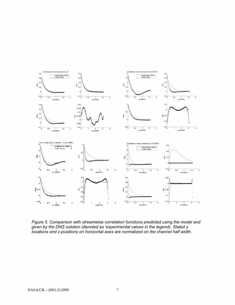
Figure 5. Comparison with streamwise correlation functions predicted using the model and given by the DNS solution (denoted as ‘experimental values in the legend). Stated y locations and z-positions on horizontal axes are normalized on the channel half width.

NASA/CR—2003-212099 7

z and y location, and correlations as a function of spanwise separation for points at the same x and y (these are all the types of correlations available in the reduced DNS data set). These correlation function comparisons are presented for four different y locations. Note that these figures use the notation u,v and w to denote the velocity components u1, u2 and u3 and thus, for example, the correlation R12 is denoted by the symbol Ruv.

At the center of the channel (y=1) the correlation functions predicted with the model generally compare well with those from the DNS. Note that the large deviations in the values of Ruv at this station from the DNS are merely the result of statistical uncertainty. The value of this correlation must be zero at the channel center, by symmetry, as predicted by the model. As y decreases the prediction between DNS and model worsens. Some of the disagreement is accounted for by the fact that correlation functions given by the DNS do not always decay to zero (as the computers intended). This lack of realism in the DNS data is most apparent in the streamwise decay of Ruu at y=0.25δ (figure 4). However, ignoring this it is apparent that, closer to the wall, the model begins to substantially under predict the rate of decay of most of the correlations. This problem is most likely associated with the fact that we are attempting to use a single, constant, lengthscale to represent the entire flow, whereas in reality the turbulence lengthscale in the channel flow decreases rapidly as the wall is approached. Figure 6 provides a somewhat different view of the correlation function predicted using the model. Plotted are the 9 components of the correlation as functions of the y-coordinates of the two points, for zero separation in z and x. While no reduced DNS data are available for comparison with these results, they are quite revealing of the problems associated with the constant lengthscale assumption.

These maps show, as expected strong correlations along the diagonals (y=y') where they represent the Reynolds stress profiles. Furthermore they show the modeled correlation functions to be symmetric about this line, as they must be. However, the Ruu and Rww correlation functions show very unrealistic behavior close to the y and y’ axes, indicating that velocity fluctuations near the wall are closely correlated with fluctuations across the entire channel, where as those near the channel center are not. This unlikely behavior turns out to be a consequence of the constant lengthscale assumption, as is demonstrated below. Additional to the calculations and analysis presented here, the constant lengthscale calculations have also been used to predict the one-dimensional proper orthogonal modes of the

y/δ

y'/δ

Figure 6. Two-point correlation maps for zero x and z separation as a function of y locations of the two points.

Ruw

Ruv

Ruu

Rvw

Rvv

Rvu

Rww

Rwv

Rwu

NASA/CR—2003-212099 8

channel flow. The grid dependence of the model solution has also been investigated. For details see Spitz (2002).

EXTENSION OF THE METHOD TO ALLOW PRESCRIPTION OF A VARIABLE LENGTHSCALE

The above results that allowing a variable lengthscale to be prescribed in the model could improve predictions. Prescribing such a lengthscale is still consistent with the ultimate application of the model, i.e. as a post processor for CFD results that provides 2-point correlation estimates, since almost all standard turbulence models used in CFD codes give as output some lengthscale as a function of position throughout the flow.

Devenport and Glegg (2001) and Devenport et al. (2001) discussed how a variable lengthscale and anisotropic decay function could be accommodated within the model framework. They argue that such variations of this type can be incorporated into the model by replacing equation (9) with,

km

ssjmniklij xx

bshbshR

∂∂+∂

='

))'()',,()(),,(()',( lnln

2 rrerrerr εε (10)

where the dependence of h() on es, the vector direction of separation, allows for the prescription of an anisotropic decay function, and the dependence on r allows for point to point changes in the prescription of the decay function form, or its lengthscale. If we are only concerned with varying the lengthscale we can write,

km

jmniklij xxbLshbLshR

∂∂+∂

='

))'())'(,()())(,(()',( lnln2 rrrrrr εε (11)

with h() still given by equation (3). As discussed by Devenport and Glegg (2001) this type of manipulation of the decay function does not alter the simple relationship between the scaling function b() and the prescribed Reynolds stress field that is the basis of the method.

As a first step we chose to prescribe L as proportional to a standard mixing length distribution. The van Driest (1956) mixing length formulation prescribes a value that increases from zero at the wall until it reaches a value of 0.09δ. From this point on the mixing length is prescribed as constant at 0.09δ. The variation in the near-wall region is given by the equation. )]/exp(1[ +++ −−= Ayym κδνl (12) where νδ is the viscous lengthscale, κ = 0.41 and A+ the van Driest constant equal to 26 For Moser et al.’s (1999) channel flow this reaches a value of 0.09δ at y/δ=0.225. The constant of proportionality between L

y/δ

y'/δ

Figure 7. Two-point correlation maps for zero x and z separation as a function of y locations of the two points,

Ruw

Ruv

Ruu

Rvw

Rvv

Rvu

Rww

Rwv

Rwu

lengthscale proportional to mixing length.

NASA/CR—2003-212099 9

and lm was chosen so that the value of L at the channel center would be the same as in the constant lengthscale calculations. Specifically, we set L=0.0053lm. Figure 7 shows the same y- correlation data plotted in figure 6, recomputed with the lengthscale varying according to this prescription. The introduction of the variable lengthscale appears to eliminate the sudden increase in the extent of the Ruu and Rww correlations close to the walls. Comparisons similar to those shown in figures 4 and 5 (see Spitz, 2002) show improved (although still imperfect) agreement between the variable lengthscale model and the DNS.

PLAN FOR FY03 Our sense of the above results, and or our progress so far, is that they provide an initial demonstration of the viability of predicting the full velocity correlation function, and thus the velocity and vorticity modes of a turbulent wall layer using the method of Devenport et al. (1999, 2001) and Devenport and Glegg (2001) modified so as to allow for the prescription of a variable lengthscale. Indeed, we are currently working on an additional variable lengthscale formulation, based on the turbulent macroscale k3/2/ε which is available from many widely used turbulence models, such as the k-ε model. However, it is also apparent that the reduced data available from Moser et al.’s (1999) simulation is limited when it comes to comparing with the model results. The reduced data includes no y-correlations and thus cannot be compared with pictures such as figure 6 and 7. Without y-correlations the DNS data cannot be used to determine the all important Proper Orthogonal or Compact Eddy modes used in noise calculations, and thus no comparisons of these are possible either.

To remedy this situation we have managed to obtain access to the raw (instantaneous) DNS results, and have begun reducing them ourselves in order to obtain the needed y-correlation information. We will also be looking at other data sets (which are also incomplete, but in other ways) for comparative data, in particular the boundary layer measurements of Adrian et al., (2000).

Once we are able to validate the modal predictions of the model, we will provide the first version of this model to the Glegg group, and begin calculations of the Wang and Moin (2000) trailing edge flow. We therefore expect to be close to the completion of the project at the end of FY03.

REFERENCES Devenport W J, Muthanna C, Ma R and Glegg S A L, "Measurement and Modeling of the Two-

point Correlation Tensor in a Plane Wake for Broadband Noise Prediction", First International Symposium on Turbulence and Shear Flow Phenomena, Santa Barbara, CA, September 12-15, 1999.

W J Devenport, C Muthanna and S A L Glegg, 2001, "Two-Point Descriptions of Wake Turbulence with Application to Noise Prediction", AIAA Journal, vol. 39, no. 12, pp. 2302-2307.

Devenport W J and Glegg S A L, 2001, "Modeling the two-point space time correlation of turbulence in a fan wake type flow", 7th AIAA CEAS Aeroacoustics Conference, 28-30th May 2000, The Netherlands.

Glegg S A L, 2001, “Noise Generated by Fans with Supersonic Tip Speeds”, Parallel grant under NRA-01-GRC-02 Aerospace Propulsion and Power Base Research and Technology Program.

Hinze J O, 1973, Turbulence, McGraw Hill, New York.

NASA/CR—2003-212099 10

Moser R D, Kim J, and Mansour N N, 1999, " Direct numerical simulation of turbulent channel flow up to Re-tau=590", Physics of Fluids, vol. 11, pp. 943-945.

Spitz N, 2002, “Prediction Of 2-Point Statistics In A Turbulent Boundary Layer”, AOE Dept., Virginia Tech, June.

Wang M and Moin P, 2000, "Computation of trailing-edge flow and noise using large-eddy simulation", AIAA Journal, vol 38, pp. 2201-2209.

NASA/CR—2003-212099 11

This publication is available from the NASA Center for AeroSpace Information, 301–621–0390.

REPORT DOCUMENTATION PAGE

2. REPORT DATE

19. SECURITY CLASSIFICATION OF ABSTRACT

18. SECURITY CLASSIFICATION OF THIS PAGE

Public reporting burden for this collection of information is estimated to average 1 hour per response, including the time for reviewing instructions, searching existing data sources,gathering and maintaining the data needed, and completing and reviewing the collection of information. Send comments regarding this burden estimate or any other aspect of thiscollection of information, including suggestions for reducing this burden, to Washington Headquarters Services, Directorate for Information Operations and Reports, 1215 JeffersonDavis Highway, Suite 1204, Arlington, VA 22202-4302, and to the Office of Management and Budget, Paperwork Reduction Project (0704-0188), Washington, DC 20503.

NSN 7540-01-280-5500 Standard Form 298 (Rev. 2-89)Prescribed by ANSI Std. Z39-18298-102

Form Approved

OMB No. 0704-0188

12b. DISTRIBUTION CODE

8. PERFORMING ORGANIZATION REPORT NUMBER

5. FUNDING NUMBERS

3. REPORT TYPE AND DATES COVERED

4. TITLE AND SUBTITLE

6. AUTHOR(S)

7. PERFORMING ORGANIZATION NAME(S) AND ADDRESS(ES)

11. SUPPLEMENTARY NOTES

12a. DISTRIBUTION/AVAILABILITY STATEMENT

13. ABSTRACT (Maximum 200 words)

14. SUBJECT TERMS

17. SECURITY CLASSIFICATION OF REPORT

16. PRICE CODE

15. NUMBER OF PAGES

20. LIMITATION OF ABSTRACT

Unclassified Unclassified

Final Contractor Report

Unclassified

1. AGENCY USE ONLY (Leave blank)

10. SPONSORING/MONITORING AGENCY REPORT NUMBER

9. SPONSORING/MONITORING AGENCY NAME(S) AND ADDRESS(ES)

National Aeronautics and Space AdministrationWashington, DC 20546–0001

Available electronically at http://gltrs.grc.nasa.gov

March 2003

NASA CR—2003-212099

E–13752

WU–708–87–23–00NAG3–2710

17

Predicting Modes of the Unsteady Vorticity Field Near the Trailing Edgeof a Blade

William J. Devenport and Nicolas Spitz

Vorticity; Aerodynamic noise; Trailing edges

Unclassified -UnlimitedSubject Category: 02 Distribution: Nonstandard

Virginia Polytechnic Institute and State UniversityAEO Department215 Randolph HallBlacksburg, Virginia 24061

Project Manager, Edmane Envia, Structures and Acoustics Division, NASA Glenn Research Center, organizationcode 5940, 216–433–8956.

Progress on predicting modes of the unsteady velocity/vorticity field of a turbulent boundary layer from Reynolds stressstatistics is described. Prediction of these modes, that provide the source terms for trailing edge noise predictions inaircraft engine fans and other configurations, will allow for the first time detailed viscous flow effects to be included insuch noise calculations. The key accomplishments of this work in FY02 are 1. The development of a Matlab code forthe prediction of modes in two- and three-dimensional boundary layers, previously applied to plane wakes; 2. Predic-tions with the code using a constant lengthscale formulation in a fully developed turbulence channel flow. Comparisonof these boundary layer predictions with available DNS simulation results; and 3. Formulation of an improved modelusing a variable lengthscale proportional to mixing length. Turbulent channel flow predictions and comparison withDNS results. This work is being carried out in continuous communication and collaboration with the Glegg researchgroup at Florida Atlantic University, which will be incorporating mode predictions into engine noise calculations.