This article was downloaded by: [University of Nebraska, Lincoln]On: 08 October 2014, At: 08:12Publisher: Taylor & FrancisInforma Ltd Registered in England and Wales Registered Number: 1072954 Registeredoffice: Mortimer House, 37-41 Mortimer Street, London W1T 3JH, UK

Canadian Water Resources Journal /Revue canadienne des ressourceshydriquesPublication details, including instructions for authors andsubscription information:http://www.tandfonline.com/loi/tcwr20

PREDICTING HEAT AND WATER FLOW IN AFREEZING/THAWING SOIL WITH NMOLG.Q. Geng , G.R. Mehuys & S.O. PrasherPublished online: 23 Jan 2013.

To cite this article: G.Q. Geng , G.R. Mehuys & S.O. Prasher (1996) PREDICTING HEAT AND WATERFLOW IN A FREEZING/THAWING SOIL WITH NMOL , Canadian Water Resources Journal / Revuecanadienne des ressources hydriques, 21:1, 69-80, DOI: 10.4296/cwrj2101069

To link to this article: http://dx.doi.org/10.4296/cwrj2101069

PLEASE SCROLL DOWN FOR ARTICLE

Taylor & Francis makes every effort to ensure the accuracy of all the information (the“Content”) contained in the publications on our platform. However, Taylor & Francis,our agents, and our licensors make no representations or warranties whatsoever as tothe accuracy, completeness, or suitability for any purpose of the Content. Any opinionsand views expressed in this publication are the opinions and views of the authors,and are not the views of or endorsed by Taylor & Francis. The accuracy of the Contentshould not be relied upon and should be independently verified with primary sourcesof information. Taylor and Francis shall not be liable for any losses, actions, claims,proceedings, demands, costs, expenses, damages, and other liabilities whatsoever orhowsoever caused arising directly or indirectly in connection with, in relation to or arisingout of the use of the Content.

This article may be used for research, teaching, and private study purposes. Anysubstantial or systematic reproduction, redistribution, reselling, loan, sub-licensing,systematic supply, or distribution in any form to anyone is expressly forbidden. Terms &Conditions of access and use can be found at http://www.tandfonline.com/page/terms-and-conditions

PREDICTING HEAT AND WATER FLOW IN AFREEZING/THAWING SOIL WITH NMOL

Submitted August 1995; accepted December 1995Written comments on this paper will be accepted until September, 1996

G.Q. Gengt, G.R. Mehuys2, and S.O. Prasher'

AbstractA program that implements the numerical method of lines (NMOL) was devel-oped for the IBM PC or compatible computer to simulate soil temperature andwater redistribution in a field soil during freezing and thawing. NMOL is a numeri-cal solution to initial-boundary value problems. In this study, NMOL was used tosolve the coupled heat and water flow in freezing/thawing soil. Measured temper-atures at the soil surface and at 17 cm depth were used as boundary conditionsof the heat flow solutions. Boundary conditions for water flow solutions werespecified as zero flux at the surface and at 17 cm depth. With this program, soilheat and water fluxes were simulated for two different days, the first when thesoil was frozen to a depth of 1.5 cm (Test 1) and the second when it was frozento 0.75 cm (Test 2). The solutions are statistically compared with field measure-ments and Crank-Nicholson solutions. The predicted temperatures and corre-sponding times had good agreement with the field measurements, while waterand ice contents predicted by NMOL were a little lower than the measured val-ues. The results obtained with NMOL were identical to those obtained with theCrank-Nicholson technique. The results demonstrate the applicability of theNMOL technique as one approach to the solution of simultaneous, partial-differ-ential eouations in soil svstems.

R6sum6Un programme utilisant la m6thode num6rique de lignes (NMOL) a 6t6d6velopp6 pour les IBM PC ou pour les ordinateurs compatibles pour simuler la

redistribution de la temp6rature et de l'eau dans le sol pendant les ph6nomdnes

de gel et d6gel. NMOL propose une solution num6rique pour les probldmes de

limite et de valeur initiale. Dans cette 6tude, NMOL est utilis6e pour r6soudre lacombinaison du flux d'eau et de chaleur dans un sol en situation de gel/d6gel.

Les temp6ratures ont 6t6 mesur6es d la surface du sol ainsi qu'd 17 cm deprofondeur pour d6finir les limites de chaleur. De m6me, les limites pour le fluxde l'eau ont 6t6 measur6es d la surface et a 17 cm. Avec ce programme, la

chaleur du sol et le flux de l'eau ont 6t6 simul6s pour deux diff6rents jours. Pourle premier jour, le sol 6tait consid6r6 gel6 jusqu'd une profondeur de 1.5 cm(Test 1), alors que pour le deuxidme jour, le sol 6tait gel6 jusqu'd 0.75 cm (Test

2). Les solutions ont 6t6 compar6es statistiquement avec les valeurs mesur6es

1. Post-Doctoral Research Fellow, Department Agricultural Engineering, McGill University,Macdonald Campus, Ste-Anne-de-Bellevue, QC

2. Associate Professor, Department of Natural Resource Sciences, McGill University, Macdonald

Campus, Ste-Anne-de-Bellevue, QC3. Associate Professor, Department of Agricultural Engineering, McGill University, Macdonald

Campus. Ste-Anne-de-Bellevue. QC

Canadian Water Resources JournalVol. 21. No. 1. 1996

69

Dow

nloa

ded

by [

Uni

vers

ity o

f N

ebra

ska,

Lin

coln

] at

08:

12 0

8 O

ctob

er 2

014

dans le champ ainsi qu'avec les solutions g6n6r6es par la technique de Crank-Nicholson. Les oredictions de temo6rature s'accordent relativement bien avecles mesures faites dans le champ. Cependant, les pr6dictions pour l'eau et laglace sont legerement inf6rieures aux mesures effectu6es dans le champ. Tousles r6sultats g6n6r6s par NMOL tendent d 6tre sensiblement diff6rents dessolutions obtenues oar la technioue de Crank-Nicholson. Ces r6sultatsd6montrent que la technique NMOL est applicable tout en pr6sentant uneapproche alternative aux probldmes d'6quations diff6rentielles partielles etsimultan6es dans le svstdme des sols.

IntroductionSoil freezing is a complex process that in-volves a dynamic balance of heat flow toand from atreezing plane. The process in-volves water migration to and into thefreezing zone, salt migration in responseto the thermal conductivity and heat ca-pacity of the soil-water system (Cary andMayland, 1972). Liquid water flow is soclosely coupled with temperature that heatflow must be considered simultaneously inany comprehensive analysis (Cary andMayland, 1972; Narlan, 1973). When achange of phase, i.e. freezing or thawingis involved, the heat and fluid flow fieldsare interdependent, and a change in direc-tion or intensity of one field affects theother. The occurrence, depth and perme-ability of frozen soil are dependent on theinterrelated processes of heat and masstransfer at the soil surface and within thesoil orofile.

Knowing whether the soil is frozen ornot is important in predicting water runoffand spring soil moisture reserve (Cary etal., 1978; Willis ef a/. 1961). An ability topredict accurately the freezing-induced re-distribution of water and heat, and the sub-sequent displacement of matter on orbeneath the ground sudace, is the goal ofscientists with interests as diverse as win-ter-hardiness of forages and long-term in-tegrity of chilled gas pipelines.

Heat and water flow in freezing soilhas been modeled using different ap-proaches (Cary ef al., 1979; Groeneveltand Kay, 1974; Harlan, 1973; Kennedyand Lielmezs, 1973; Osterkamp, 1987).The advent of the computer has acceler-ated the develooment of models to simu-

70

late heat and water flow and estimatefrost depth (Guymon and Luthin, 1974;Hayhoe et al., 1983; Jame and Norum,1980; Konrad and Duquennoi, 1993;Kung and Steenhuis, 1986). One of thewidely-used models was devised byHarlan (1973), using an analogy betweenthe mechanism of water transport in par-tially frozen soils and that in unsaturatedsoils. By use of this analogy, a Darcianapproach was applied to the analysis ofcoupled heat-fluid transport in porousmedia with freezing and thawing. With theaid of a numerical model, Harlan exam-ined the freezing-affected soil-water re-distribution and infiltration to frozen soilusing the coupled heat and water flowequations. Later, Taylor and Luthin(1978), Jame and Norum (1980), andPikul et a/. (1989) also simulated unsatu-rated water flow when coupled heat andwater flow and phase change took placein the laboratory or in the field, using amodified form of the model presented byHarlan (1973). Under unsaturated condi-tions, water flow is driven by both the gra-dient in unfrozen water content, whichimplicitly represents the matric potential,and an appropriate soil water sink orsource term that is based on the rate ofchange of ice content within the freezingsoil. Pikul et a/. used an experimental orderived relationship of unfrozen watercontent to subzero temperature to couplethe heat and water flow equations and adifferent technique to attain the ratechange of ice.

The objective of this study is to intro-duce the numerical method of lines

Revue canadienne des ressources hydriquesVol. 21. No. 1. 1996

Dow

nloa

ded

by [

Uni

vers

ity o

f N

ebra

ska,

Lin

coln

] at

08:

12 0

8 O

ctob

er 2

014

(NMOL) to the solution of coupled heatand mass transfer processes during freez-ing/thawing of soil.

The NMOL TechniqueThe Numerical Method of Lines (NMOL)was developed by Schiesser (1977) tosolve partial differential equations andmixed ordinary and partial differentialequations. lt is a numerical solution to ini-tial-boundary value problems, based onclassical implicit finite difference algo-rithms. Prasher and Madramootoo (1987)first used the NMOL technioue to solve ini-tial-boundary value problems in soil hy-drology on an IBM PC or compatiblecomputer. They demonstrated the tech-nique by solving initial-boundary valueproblems in the design of drainage andsub-irrigation systems (Prasher andMadramootoo, 1987).

The problem-domain is discretized, asin the finite difference method, so that thegoverning partial differential equation isvalid equally at all the nodal points. Whilethe spatial derivatives in the differentialequation are approximated by algebraicexpressions based on the Taylor series,the time derivative is left alone. This re-sults in a set of ordinary differential equa-tions, one for each nodal point, which canbe solved by one of the many availablemethods of solving ordinary differentialeouations.

The following algorithms are availableat the present time in the NMOL softwarepackage: (1) Runge Kutta Euler, (2)Runge Kutta Niesse, (3) Runge KuttaMerson, (4) Runge Kutta Tanaka-4, (5)Runge Kutta Tanaka-s, (6) Runge KuttaChai, (7) Runge Kutta England, (8) RungeKutta Wes-4/1, (9) Runge Kutta Wes-4/2,(10) Runge Kutta Wes-413, (11) RungeKutta Wes-4/4, (12) Runge Kutta Wes-4/5,(13) Runge Kutta Wes-5/1, and (14)Runge Kutta Wes-5/2.

For most problems, any algorithm fromthe above list can be used. The main fea-ture of this method is that the oroceduredoes not change from one problem to an-

Canadian Water Resources JournalVol.21, No. 1. 1996

other and from one-dimensional to two- orthree-dimensional problems. Moreover,with this approach, the time spent on de-veloping numerical solutions is reducedfrom months to days.

The programming effort in the NMOLtechnique is minimal. Only three subrou-tines, lNITAL, DERV and PRINT, are writ-ten by the user in the FORTRAN-77language. The subroutine INITAL containsthe initial conditions of the problem, whichis called only once by the main program.Therefore, any other calculations thatneed to be done once for a given run orinitializations can be included in this sub-routine. The subroutine DERV is calledmany times by the main program. lt, inturn, calls subroutines that approximatespatial derivatives. The boundary condi-tions are also established in DERV. Noimaginary nodes are needed at theboundary, as in the finite differencemethod. In DERV, the derivatives of thedependent variables are calculated withrespect to time and sent to the mainNMOL program (an initial-value integra-tor). The subroutine PRINT prints interme-diate or final results. The format of theprinted output, generated by the numeri-cal solution of the problem, is given in thissubroutine. In most cases, the main pro-gram requires three input data lines con-taining information with respect to thenumber of nodal points in the region, algo-rithm to be used, tolerance, printing inter-val, etc. (Prasher and Madramootoo,1987; Schiesser, 1977).

Application of NMOLA program that implements the NMOLtechnique was developed for the IBM PCor compatible computer with a mathemati-cal co-processor to solve initial-boundaryproblems of coupled heat and water flowin a freezing soil system. This programwas run against the field measurementsand numerical solutions given by Pikul efa/. (1989), in which they used the Crank-Nicholson method to obtain numerical so-lutions. The field treatment was a 40- bV

71

Dow

nloa

ded

by [

Uni

vers

ity o

f N

ebra

ska,

Lin

coln

] at

08:

12 0

8 O

ctob

er 2

014

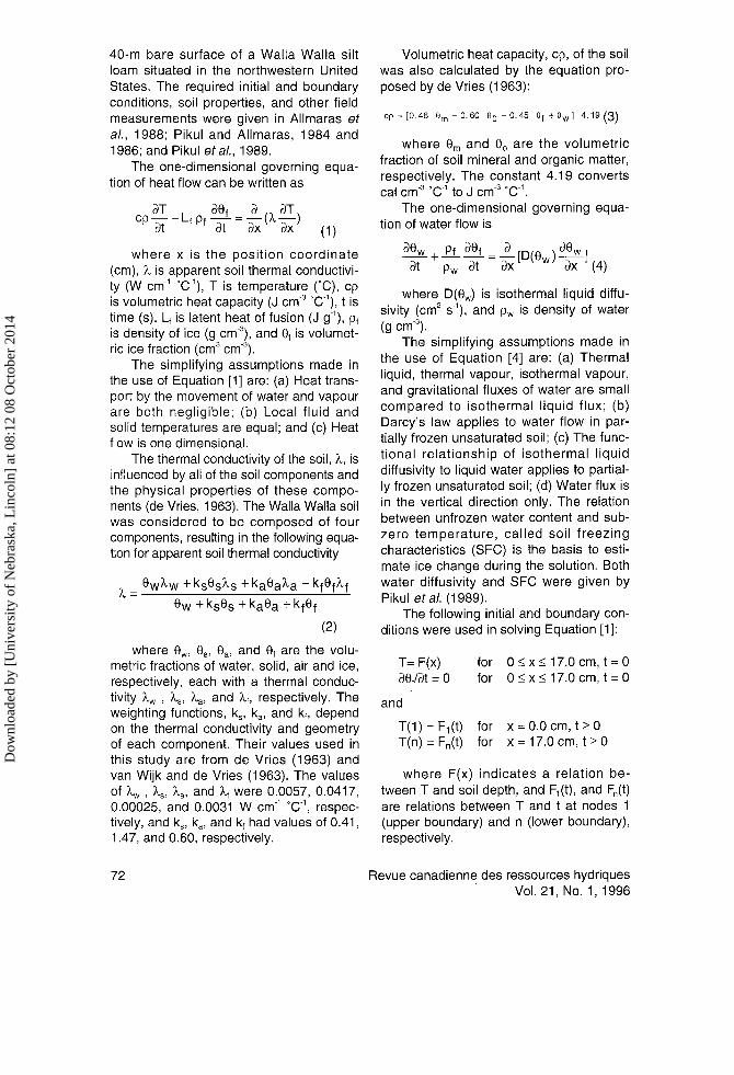
40-m bare surface of a Walla Walla siltloam situated in the northwestern UnitedStates. The required initial and boundaryconditions, soil properties, and other fieldmeasurements were given in Allmaras eta/., 1988; Pikul and Allmaras, 1984 and1986:and Pikulef a/.. 1989.

The one-dimensional governing equa-tion of heat flow can be written as

ar dor a ." ar.co__L+o+_=_( _)'at " at 3x' dx' (1)

where x is the oosition coordinate(cm), )" is apparent soil thermal conductivi-ty (W cm-' 'C'), T is temperature ("C), cpis volumetric heat capacity (J cm-' 'C-';, t istime (s), L, is latent heat of fusion (J g-'), p1

is density of ice (g cm'), and 0, is volumet-ric ice fraction (cmt cm-t).

The simplifying assumptions made inthe use of Equation [1] are: (a) Heat trans-port by the movement of water and vapourare both negligible; (b) Local fluid andsolid temperatures are equal; and (c) Heatflow is one dimensional.

The thermal conductivity of the soil, 1,, isinfluenced by all of the soil components andthe physical properties of these compo-nents (de Vries, 1963). The Walla Walla soilwas considered to be comoosed of fourcomponents, resulting in the following equa-tion for apparent soil thermal conductivity

^

_ Ow)"w + ksOsl"s + ka0al"a + kf Of),f

0* +ksOs +ksOs +k101

(2\

where 0*, 0., 0u, and 0t are the volu-metric fractions of water, solid, air and ice,respectively, each with a thermal conduc-tivity )"" , tr., tr", and \, respectively, Theweighting functions, k", k", and k1, dependon the thermal conductivity and geometryof each component. Their values used inthis study are from de Vries (1963) andvan Wijk and de Vries (1963). The valuesof \ , ),", 1.", and ln were 0.0057, 0.0417,0.00025. and 0.0031 W cm-' 'C-', respec-tively, and k", ku, and k, had values of 0.41 ,

1 .47, and 0.60, respectively.

72

Volumetric heat capacity, cp, of the soilwas also calculated by the equation pro-posed by de Vries (1963):

cp = [0.46 em + 0.60 eo + 0.45 01 + e* J a.19 ($)

where 0. and 0o are the volumetricfraction of soil mineral and organic matter,respectively. The constant 4.19 convertscal cm.'C-tto J cm-3'C-1.

The one-dimensional governing equa-tion of water flow is

do' * Pt dot = E tora,.,)dt*lat p* Et Dx' "" dx ' (a)

where D(0") is isothermal liquid diffu-sivity (cm'? s-'), and p* is density of water(g cm').

The simplifying assumptions made in

the use of Equation [4] are: (a) Thermalliquid, thermal vapour, isothermal vapour,and gravitational fluxes of water are smallcompared to isothermal liquid flux; (b)Darcy's law applies to water flow in par-tially frozen unsaturated soil; (c) The func-tional relationship of isothermal liquiddiffusivity to liquid water applies to partial-ly frozen unsaturated soil; (d) Water flux is

in the vertical direction only. The relationbetween unfrozen water content and sub-zero temperature, called soil freezingcharacteristics (SFC) is the basis to esti-mate ice change during the solution. Bothwater diffusivity and SFC were given byPikulef a/. (1989).

The following initial and boundary con-ditions were used in solving Equation [1]:

T= F(x)d0y'Dt = 0

ano

for 0<x<17.0cm,t=0for 0<x<17.0cm,t=0

T(1)= F1(t) for x = 0.0 cm, t > 0T(n) =F"(t) for x=17.Ocm,t>0

where F(x) indicates a relation be-tween T and soil depth, and F (t), and F"(t)

are relations between T and t at nodes 1

(upper boundary) and n (lower boundary),respectively.

Revue canadienne des ressources hydriquesVol. 21. No. 1 . 1996

Dow

nloa

ded

by [

Uni

vers

ity o

f N

ebra

ska,

Lin

coln

] at

08:

12 0

8 O

ctob

er 2

014

The one-dimensional space domainwas evenly subdivided based on the num-ber of nodal points which was given in thesubroutine lNITAL. In this case, there were69 nodal ooints with a distance of 0.25 cmbetween two nodal points.

The following initial and boundary con-ditions were used in solving Equation [4]:

0* -- G(x)ae/at = 0

ano

30*/Dx = 0DO./Ex = 0

for 0 < x < 17.0 cm, t = 0for 0<x<17.0cm,t=0

for x=0.0cm,t>0for x=17.Ocm,t>0

where G(x) describes the relation of 0*and soil depth. The boundary conditionsfor the water flow solution were specifiedas zero flux at the too and bottom of thecolumn during both freezing and thawing.All F(x), Fr(t), F"(t), and G(x) were mea-sured in the field (Pikul ef a/., 1989).

The amount of water remaining un-frozen in a soil is often considerable, de-creases with the temperature, and varieswith soil type (Williams and Burt, 1974).The transoort of water and heat in a frozenporous medium is complicated by the pres-ence of water in the solid ohase and thefact that the liquid water content is stronglytemperature dependent (Kay andGroenevelt, 1974). Previous studies haveemployed different strategies for estimatingthe ice change, AOs. Harlan (1973) suggest-ed that an optimization procedure be incor-porated into the computational scheme thatiterates between the heat transfer equationand mass transfer equation. Taylor andLuthin (1978) proposed a coefficient whosemagnitude is adjusted between time stepsso that calculated water content agrees withthat given by the experimental relationshipbetween unfrozen water content and sub-zero temperature. Jame and Norum (1980)first estimated Aer by the heat transferequation using apparent soil heat capacity,which includes latent heat of fusion.Iteration was then carried out between heat

Canadian Water Resources JournalVol.21. No. 1. 1996

and water flow equations, but the criteriaused to stoo the iteration were not dis-cussed. Pikul ef a/. (1989) determined A06

by estimating the heat change during thetime step and equating the heat loss/gain to

a volumetric fraction of ice loss/gain. Theirproblem was that the soil water diffusivityneeded to be multiplied by a factor of 0.1 tobetter fit the field measurement.

In this study, A01 was estimated in thesubroutine DERV. Whenever the tempera-ture becomes less than zero, the calculatedliquid water content is adjusted to agreewith that given by the experimental relation-shio between unfrozen water content andsubzero temperature (the SFC). The differ-ence between them is the ice change Aer.

The accumulated ice content is increasedor decreased based on the ice change.

The measured and Predicted valueswere statistically compared by calculatingthe standard error and mean relativeerror, which are computed by the follow-ing equations:

where S.E. is the standard error; Yo is

the predicted value of a given point; Y, is

the measured value of that point; n is thenumber of points.

r (Y^ - Y-)tr =_\i'n ""100-'- nu Ym (6)

where E, is the mean relative error (k).

Results and DiscussionTest 1:

Soil temoerature and water and ice contentwere simulated with the developed pro-gram that implements the NMOL techniqueusing the field measurements of March 21

and 22, 1982 (Pikul et al., 1989) as the cor-

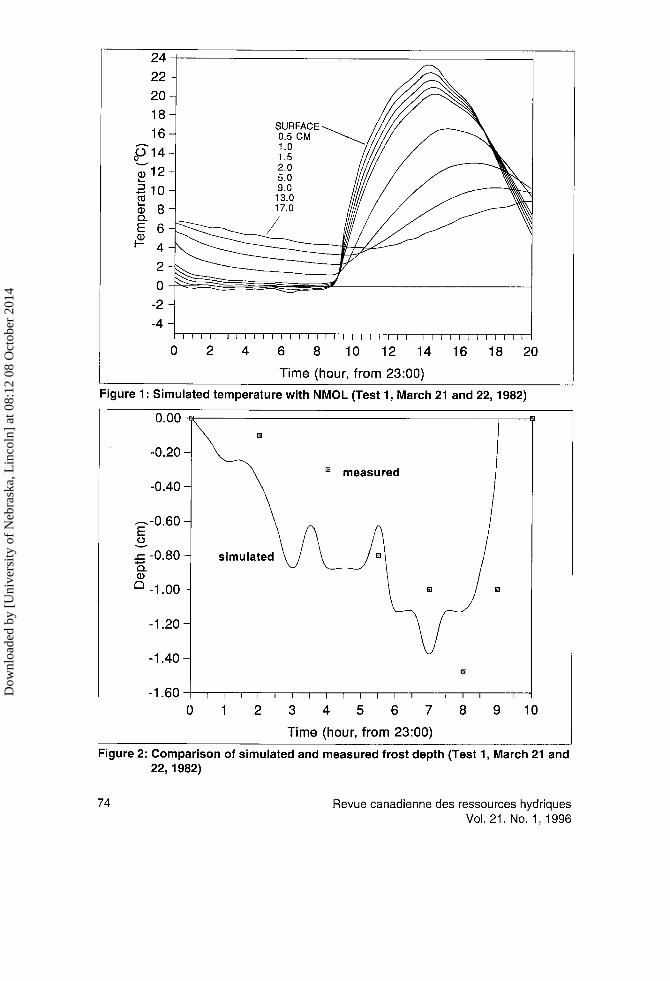
responding initial and boundary conditions.The simulated temperature distributionswith NMOL are shown in Figure 1. The sur-face (upper boundary) and bottom (lower

(5)

r(Yp - Yr)2n

73

Dow

nloa

ded

by [

Uni

vers

ity o

f N

ebra

ska,

Lin

coln

] at

08:

12 0

8 O

ctob

er 2

014

24

22

20

18

16

9t+a12J {nt tv

b8E6,o

4

2

0

-2

-4

38101214Time (hour, from 23:00)

SURFACE0.s cM1.0t.J2.05.0on13.017.0

Figure 1 : Simulated temperature with NMOL (Test 1, March 21 and 22, 1982)

0.00

-0.20

-0.40

^-0.60E

I-o.aoo-oo -t.oo

-1.20

-1.40

-1.6034567Time (hour, from 23:00)

Figure 2: Comparison of simulated and measured frost depth (Test 1, March 21 and22,1982)

Revue canadienne des ressources hydriquesVol.21. No. 1.1996

74

Dow

nloa

ded

by [

Uni

vers

ity o

f N

ebra

ska,

Lin

coln

] at

08:

12 0

8 O

ctob

er 2

014

boundary) temperatures are field measure-ments. Maximum predicted soil tempera-tures at 1.0. 2.0. and 9.0 cm occurred at14.3, 14.5 and 16.5 h, respectively. Bycomparison, maximum soil temperaturesmeasured and predicted by Pikul et a/.(1989) with the Crank-Nicholson method atthe same depths occurred at 14.0, 14.0and 16.3 h and 13.5, 13.6, 15.8 h, respec-tively. The maximum soil temperatures pre-dicted by NMOL occurred a little later,while those predicted by Crank-Nicholson alittle earlier than the field measurements.The standard error of the predicted time byNMOL from the measured time was 0.4 h,

while the mean relative error was 2.3oh.The maximum soil temperatures predictedat those depths by Pikul et a/. (1989) withCrank-Nicholson were about 21.5, 20.0,and 13.0"C, respectively, while those byNMOLwere 21 .7,2O.3 and 13.0'C, respec-tively. The differences between these twopredictions of temperature were extremelysmall and the mean relative error between

them was only 0.81%. The maximum neg-ative temperature measured at the surfaceoccurred at 6.5 h. The maximum negativetemperature at 1 cm predicted by bothNMOL and Crank-Nicholson occurredaround 7 h. The temperature values pre-

dicted by the two numerical solutions werevery similar. Simulated soil temperatureand related time predicted bY NMOLagreed well with the field measurementsand the Crank-Nicholson solutions basedon the S.E. and E, values.

The frost depths measured and Pre-dicted with NMOL are shown in Figure 2

for March 21 and 22, 1982. The soil wasconsidered frozen when the temperatureat a node was less than 0'C. Generally,the predicted frost depth was a littlegreater than the measured depth beforethe maximum frost penetration was at-tained. This could be due to a frost tem-perature set a little too high or theincorrectness of frost measurement sincethe frost depth was determined visually.

0.45

0.40

0.35

0.30

0.25

0.20

o-

I

I

18 2068101214Time (hour, from 23:00)

16

Figure 3: Comparison of simulated and measured ice and water content (0 to 1 cmof Test 1, March 21 and22,1982)

Canadian Water Resources JournalVol.21, No.1,1996

75

Dow

nloa

ded

by [

Uni

vers

ity o

f N

ebra

ska,

Lin

coln

] at

08:

12 0

8 O

ctob

er 2

014

The standard error of frost deoth was 0.3cm and the mean relative error 0.1%. Themaximum predicted f rost penetrationcame earlier than the measured one. Themaximum measured frost deoth was 1.5cm and occurred at I h. Those predictedby NMOL and Crank-Nicholson were both1.4 cm, respectively, and occurred at 7 h

and from 6.3 to 8 h, respectively. Bothmethods predicted that complete soilthawing occurred at t h, which was mea-sured at 9.5 h. The predicted values off rost depth using these two methodsshowed little difference and their meanrelative error was only 0.02"k.

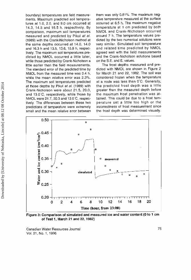
The predicted and measured ice andwater content in the 0- to 1-cm soil layerare shown in Figure 3 for March 21 and22, 1982. Like Pikul's prediction, differ-ences between measured and oredictedice and water contents were larger thanthose of temperature. Generally, the pre-dicted water and ice contents were a littlelower than measured values. The stan-

dard error of the NMOL from the measure-ment was 0.05 cm3/cm3 and the relativeerror -3.8%. The maximum water and icecontents measured were 0.49 and oc-curred at 7.5 h. By comparison, the maxi-mum values predicted by NMOL andCrank-Nicholson were 0.43 and 0.45 andboth occurred at 8 h, respectively. Thepredictions from the two methods weresimilar, with a -5.8% mean relative error.Pikul ef a/. (1989) explained that the un-derestimation of ice and water contentcould be due to the incorrectness of mea-sured water diffusivity. Another reasoncould be that the frost oenetration waspredicted to be greater.

Test 2:

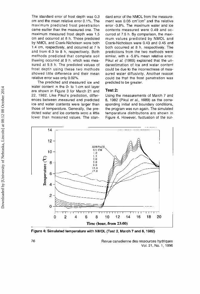
Using the measurements of March 7 and8, 1982 (Pikul ef a/., 1989) as the corre-sponding initial and boundary conditions,the program was run again. The simulatedtemoerature distributions are shown inFigure 4. However, fluctuation of the sur-

12

10

p;8Ebb

f4

68101214Time (hour, from 23:00)

SURFACE0.5 cM1.01.52.05.09.013.017.0

Figure 4: Simulated temperature with NMOL (Test 2, March 7 and 8, 1982)

Revue canadienne des ressources hydriquesYol.21. No.1.1996

76

Dow

nloa

ded

by [

Uni

vers

ity o

f N

ebra

ska,

Lin

coln

] at

08:

12 0

8 O

ctob

er 2

014

face temoerature occurred several timesduring March 7 and 8. Maximum predictedsoil temperature at 1 cm dePth was11.7'C and occurred at 16.0 h. By com-parison, the maximum soil temperaturesmeasured and predicted by Pikul ef a/(1989) with Crank-Nicholson were also11.7"C at that depth and occurred at 16.0h. The standard error of temperature pre-

dicted by NMOL from measurements at 1

cm depth were 0.2'C and mean relativeerror was 1.0%. The other two tempera-ture peaks at 1 cm depth were 8.3 and11.2'C at 11.5 and 14.5 h, respectively,for NMOL orediction and 8.2 and 11.0'Cat 11.5 and 14.5 h, respectivelY, forCrank-Nicholson. The mean relative errorof temperatures predicted by the twomethods was 1.0%. The maximum nega-tive temperature at 0.5 cm predicted bythe two methods occurred at 8.5 h. Thetemperatures predicted by the two meth-ods were very similar. Even in the pres-

ence of temperature fluctuations, the soil

temperature simulated by NMOL fit thefield measurement extremely well.

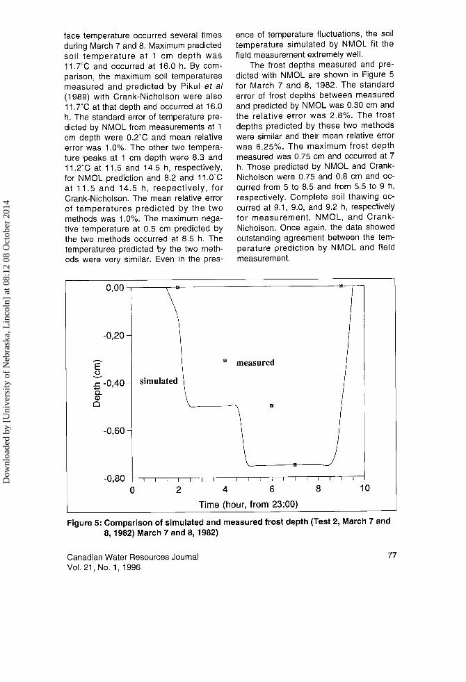
The frost depths measured and Pre-dicted with NMOL are shown in Figure 5

for March 7 and 8, 1982. The standarderror of frost depths between measuredand predicted by NMOL was 0.30 cm and

the relative error was 2.8%. The frostdepths predicted by these two methodswere similar and their mean relative errorwas 6.25"/o. The maximum frost depthmeasured was 0.75 cm and occurred at 7h. Those predicted by NMOL and Crank-Nicholson were 0.75 and 0.8 cm and oc-

curred from 5 to 8.5 and from 5.5 to t h,

respectively. Complete soil thawing oc-

curred at 9.1, 9.0, and 9.2 h, respectivelyfor measurement, NMOL, and Crank-Nicholson. Once again, the data showedoutstanding agreement between the tem-perature prediction by NMOL and fieldmeasurement.

E9o-oo

46Time (hour, from 23:00)

Figure 5: Comparison of simulated and measured frost depth (Test 2, March 7 and8,1982) March 7 and 8,1982)

Canadian Water Resources JournalVol. 21. No. 1. 1996

77

Dow

nloa

ded

by [

Uni

vers

ity o

f N

ebra

ska,

Lin

coln

] at

08:

12 0

8 O

ctob

er 2

014

0.50

? 0.45

I

E o.4o

'- u.J5

$ o.eo

0.2568101214Time (hour, from 23:00)

18 20

simulated

Figure 6: Comparison of simulated and measured ice and water content(0 to 1 cm of Test 2, March 7 and 8, 1 982)

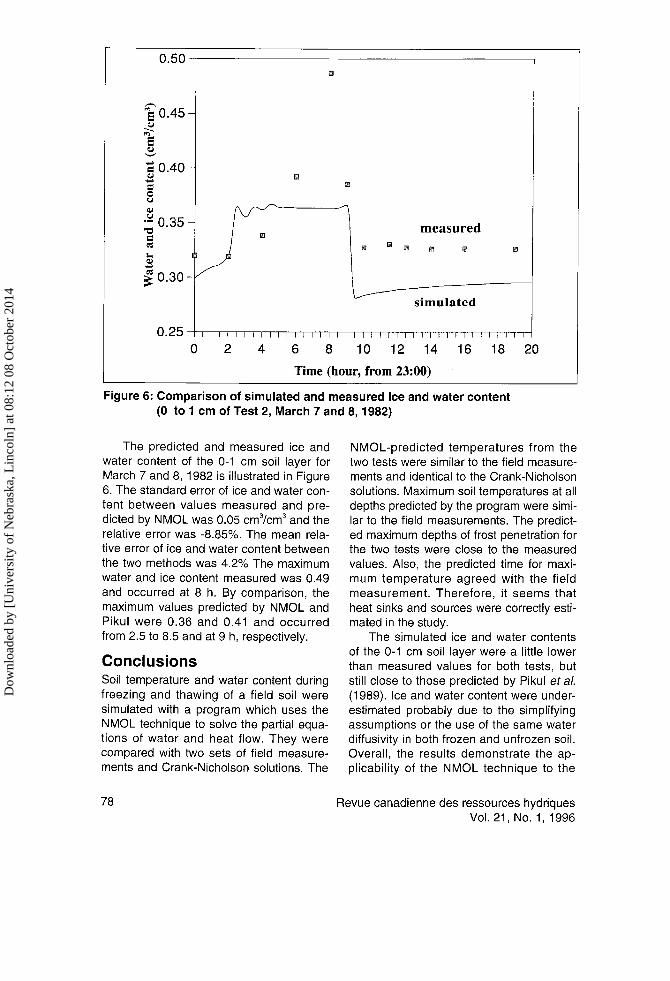
The predicted and measured ice andwater content of the 0-1 cm soil layer forMarch 7 and 8, 1982 is illustrated in Figure6. The standard error of ice and water con-tent between values measured and ore-dicted by NMOL was 0.05 cm3/cm3 and therelative error was -8.85%. The mean rela-tive error of ice and water content betweenthe two methods was 4.2o/o The maximumwater and ice content measured was 0.49and occurred at 8 h. By comparison, themaximum values predicted by NMOL andPikul were 0.36 and 0.41 and occurredfrom 2.5 to 8.5 and at t h, respectively.

GonclusionsSoil temperature and water content duringfreezing and thawing of a field soil weresimulated with a program which uses theNMOL technique to solve the parlial equa-tions of water and heat flow. They werecompared with two sets of field measure-ments and Crank-Nicholson solutions. The

td

NMOL-predicted temperatures from thetwo tests were similar to the field measure-ments and identical to the Crank-Nicholsonsolutions. Maximum soil temperatures at alldepths predicted by the program were simi-lar to the field measurements. The oredict-ed maximum depths of frost penetration forthe two tests were close to the measuredvalues. Also, the predicted time for maxi-mum temperature agreed with the fieldmeasurement. Therefore, it seems thatheat sinks and sources were correctly esti-mated in the study.

The simulated ice and water contentsof the 0-1 cm soil layer were a little lowerthan measured values for both tests, butstill close to those predicted by Pikul et al.(1989). lce and water content were under-estimated probably due to the simplifyingassumotions or the use of the same waterdiffusivity in both frozen and unfrozen soil.Overall, the results demonstrate the ap-plicability of the NMOL technique to the

Revue canadienne des ressources hydriquesVol.21. No. 1.1996

Dow

nloa

ded

by [

Uni

vers

ity o

f N

ebra

ska,

Lin

coln

] at

08:

12 0

8 O

ctob

er 2

014

solution of initial and boundary-valueproblems associated with coupled heatand water flow in soil systems. Also, thetime reouired to obtain NMOL solutions is

considerably less than for other numericalsolutions.

AcknowledgementsThe authors would like to express theirappreciation to Dr. J,L. Pikul, Jr. and hiscolleagues for the use of their data in thisstudy.

ReferencesAllmaras, R.R., J.L. Pikul Jr., J.M. Kraft,and D.E. Wilkins. 1988. "A method formeasuring incorporated crop residue andassociated soil properties." SorT ScienceSociety of America Journal, 521 1 28-1 1 33.

Cary, J.W. and H.F. Mayland. 1972. "Saltand water movement in unsaturated'frozen soil." Soll Science Society ofAmerica P roceedi ngs, 36:549-555.

Cary, J.W, G.S. Campbell and R.l.Paoendick. 'l 978. "ls the soil frozen ? Analgorithm using weather records." WaterResources Research, 1 4, 1 1 17 -1 122.

Cary, J.W, R.l. Papendick and G.S.Camobell. 1979. "Water and salt move-ment in unsaturated frozen soil: principlesand field observations." Sol/ ScienceSociety of America Journal,43, 3-8.

de Vries, D.A. 1963. "Thermal propertiesof soils." /n W.R. van Wijk (ed) Physics ofthe plant environmenf. North-Holland,Amsterdam, 210-235.

Groenevelt, P.H. and B.D. Kay. 1974. "Onthe interaction of water and heat transoodin frozen and unfrozen soil: ll. The liouidphase." Soil Science Society of AmericaP roceedi ngs, 38, 4O0-4O4.

Guymon, G.L. and J.N. Luthin. 1974. "A

coupled heat and moisture transportmodel for Arctic soils." Water ResourcesResearch 10,995-1001.

Canadian Water Resources JournalVol.21. No. 1. 1996

Harlan, R.L. 1973. "Analysis of coupledheat{luid transport in partially frozen soil."Water Resources Research, 9, 1314-1323.

Hayhoe, H.N., G.C. Topp and S.N. Edey.

1983. "Analysis of measurement and nu-merical schemes to estimate frost andthaw penetration of a soil." CanadianJournal of Soil Science, 63, 67-77.

Jame, Y.W. and D.l. Norum. 1980. "Heat

and mass transfer in a freezing unsaturat-ed porous medium." Water ResourcesResearch. 1 6. 81 1 -81 9.

Kay, B.D. and P.H. Groenevelt. 1974. "On

the interaction of water and heat transpotlin frozen and unfrozen soil: l. Basic theory,the vapour phase." Soil Science Society ofAmerica Proceedings, 38, 395-400.

Kennedy, G.F. and J. Lielmezs. 1973."Heat and mass transfer of freezing water-soil system." Water Resources Research,9:395-400.

Konrad, J.M. and C. Duquennoi. 1993."A model for water transport and ice lens-ing in freezing soil." Water ResaurcesRese arch. 29. 31 Og -31 24.

Kung, S.K.J. and T.S. Steenhuis. 1986."Heat and moisture transfer in a partlyfrozen nonheaving soil." Soll ScienceSociety of America Journal, 50:1 1 1 4-1 122.

Osterkamp, T.E. 1987. "Freezing andthawing of soils and permafrost containingunfrozen water or brine." Water ResourcesR e s ea rch, 23:227 9-2285.

Pikul, J.L. Jr. and R.R. Allmaras. 1984."A field comparison of null-aligned andmechanistic soil heat flux." Sol/ ScienceSociety of America Journal,48, 1207-1214.

Pikul, J.L. Jr. and R.R. Allmaras, 1986."Physical and chemical properties of aHaploxeroll after fifty years of residuemanagemenl." Soil Science Society ofAmerica Journal. 50, 21 4-219.

Pikul, J.L. Jr., L. Boesma, and R.W.Rickman. 1989. "Temoerature and waterprofiles during diurnal soil freezing and

79

Dow

nloa

ded

by [

Uni

vers

ity o

f N

ebra

ska,

Lin

coln

] at

08:

12 0

8 O

ctob

er 2

014

thawing: field measurements and simula-tion." Soil Science Societv of AmericaJournal.53. 3-1 0.

Prasher, S.O. and C. Madramootoo. 1987."Application of the numerical method oflines (NMOL) in soil hydrology."Tran sactions A54E 30: 1 98-200.

Schiesser, W.E. 1977. An introduction tothe numerical method of lines integrationof partial differential equations. LehighUniversity and Naval Air DevelopmentCenter, Bethlehem, Pennsylvania.

Taylor, G.S. and J.N.Luthin. 1978."A model for coupled heat and moisture

transfer during soil freezing." CanadianGeotechnical Journal, 1 5, 548-555.

van Wijk, W.R. and D.A. de Vries. 1963,"The atmosphere and the soil." /n W.R.van Wijk (ed), Physics of the plant environ-menf. North-Holland, Amsterdam, 1 7-59.

Williams, P.J. and T.P. Burt. 1974."Measurement of hydraulic conductivity oflrozen soils." Canadian GeotechnicalJournal. 1 1. 647-650.

Willis, W.O., C.W. Carlson, J. Alessi andH.J. Hass. 1961. "Depth of freezing andspring runoff as related to fall soil-moisturelevel." Sol/ Science Societv of AmericaJournal. 41. 115-123

Revue canadienne des ressources hydriquesVol.21. No. 1.1996

80

Dow

nloa

ded

by [

Uni

vers

ity o

f N

ebra

ska,

Lin

coln

] at

08:

12 0

8 O

ctob

er 2

014