Purdue UniversityPurdue e-PubsDepartment of Electrical and ComputerEngineering Technical Reports

Department of Electrical and ComputerEngineering

11-1-1989

Predicting Fault Transients on UndergroundResidential Distribution Systems - A Project of thePurdue Electric Power CenterL. M. RuxPurdue University

W. L. WeeksPurdue University

Follow this and additional works at: https://docs.lib.purdue.edu/ecetr

This document has been made available through Purdue e-Pubs, a service of the Purdue University Libraries. Please contact epubs@purdue.edu foradditional information.

Rux, L. M. and Weeks, W. L., "Predicting Fault Transients on Underground Residential Distribution Systems - A Project of the PurdueElectric Power Center" (1989). Department of Electrical and Computer Engineering Technical Reports. Paper 686.https://docs.lib.purdue.edu/ecetr/686

Predicting Fault Transients on Underground Residential Distribution Systems

A Project of the Purdue Electric Power Center

L. M. Rux W. L. Weeks

TR-EE 89-63 November, 1989

School of Electrical EngineeringPurdue UniversityWest Lafayette, Indiana 47907

Predicting Fault Transients

■ on'

Undergronnd Pesidential Distribution Systems

A Project of the

Purdue Electric Power Center

‘ ■ Wr

by

Lorelynn M. Rux

Graduate Student

Prof. W. L. Weeks

Advisor

December, 1989

. A b s t r a c t

This thesis addresses the problem of calculating and utilizing the voltage and current transients that may occur in underground residential distribution (URD) systems. A computational model for such systems is proposed and evaluated by comparisons to experimental results. The propagation characteristics of standard URD cables are complex but central to the computational model. The specific objective of this study was to determine whether a relatively simple approximation for the cable propagation constant is accurate enough that, when incorporated into the computational model for the transients resulting from a fault in the system, the resulting fault transient can be utilized to locate the fault.

The conclusion is that over a frequency range of approximately 0.1 to 10 MHz, the computational model does provide a useful description of the transients. The approximation for the cable propagation constant does seem to provide adequate information about the variation with frequency of the phase constant and the attenuation constant when plausible ad hoc values of the parameters are included. The computational model is simple and quick to evaluate. It is based on standard lattice diagram analysis of the multiple reflections in the system. The model provides an approximation to the impulse response of the system, when the impulse is applied at various positions In the system.

I

CHAPTER I - UNDERGROUND POWER DISTRIBUTION

1.1 Introduction

In the early to mid-1960's electric utility companies began to shift their focus from overhead to underground installations for residential power distribution systems. The reduction of overhead lines and appearance of underground networks brought a favorable response from consumers. The practice of undergrounding distribution equipment has continued to flourish and virtually all new subdivisions and commercial businesses are being served by underground systems. [1]

In most cases it hasn't been practical to replace existing overhead lines with buried cables. However, at new installations the costs associated with underground distribution systems are feasible when compared with the costs for overhead networks. [2] And although underground circuits have their own disadvantages they are relatively immune to some of the problems faced by overhead lines, such as power-pole accidents and damage caused by lightning, snow and wind storms.

,, Presently, there are more than a million miles of underground residential distribution (URD) cable buried in the United States. [1] The beneficial combination of aesthetics, safety and economics ensures that the demand for URD will continue to increase in the future.

1.2 URD Cables and Equipment

A primary single-phase concentric-neutral underground cable is shown in Figure 1.1. Underground power cables typically consist of one or more insulated conductors, enclosed in a protective sheath. The neutral conductors often surround the insulation in a helical pattern, as shown, and may be also be protected against the environment by an outer sheath. Power cables are classified according to their design and the materials used in their construction.

Conductors are normally made of solid or stranded copper or aluminum, with Stranded conductors giving more flexibility to the finished cable. Round stranded conductors may be compacted to reduce the cable diameter, although this also reduces flexibility.

Insulation materials include oil-impregnated paper, natural and synthetic rubber compounds, and plastics. A common insulation material is crosslinked polyethylene (XLPE), obtained by chemically crosslinking polyetheylene with a variety of organic chemicals. Among the many useful properties of polyethylene is its ability to be extruded over a conductor with excellent results. The crosslinking extends the operating temperature of the insulation to 90C [3].

Sheaths and jackets prolong the life of the insulation and conductors by guarding against mechanical and corrosive damage. Sheathing materials include metals such as lead, aluminum and iron, and semiconducting polymers such as chloroprene and polyvinylchloride (PVC).

The combination of conducting, insulating and sheath materials produces a cable with unique physical, mechanical and electrical properties. Figure 1.2 shows a cross- section of a typical single-conductor cable.

In addition to the power cables, an underground distribution system will generally include other auxiliary equipment. Among those components are:

1. Splices and connectors, for joining two cables.2. Terminations, where cables are connected to overhead lines or other electrical

■ :v; apparatus.3 . URD transformers, for lowering voltages before distribution to the customer.4. Ducts and manholes, in underground systems where cables are not directly buried.5. Risers, which connect the underground system to die overhead network;

Figure 1.3 shows an example of the layout of an underground residential distribution system consisting Of buried primary, and secondary cables, and a distribution transformer.

3

PROTECTIVE JACKET

SE JiM-GO NOUCTIN G HIGH VOLTAGE SHIELDING INSULATIONLAVER /

CONCENTRIC NEUTRAL STRAN DS

STR AND SHIELDING LAYER

Figure 1.1 Single phase concentric neutral underground cable.

CO ND U CTO R

INSUi-ATfONGROU N DEDSHEATH

Figure 1.2 Cross-section of a single conductor cable.

5

PRIMARY— ■ — SECONDARY

'fO -* AREA [ T I TRANSFORMER

Figure 1.3 Underground residential distribution layout.

1.3 Cable Faults

A 1985 nationwide survey of electric utilities indicted that the "major underground distribution problems facing electric utilities" were the premature failure of primary distribution cables and the repair of direct-buried cables in ieveloped areas. [4]

The Service life of URD primary cable (15-35kV) is shorter than the 40 years expected by the utilities [5J. Efforts are underway to present premature dielectric failures and improve reliability. Among the methods being investigated are I) protecting the insulation from defects and contamination during the manufacturing process, and 2) modifying cable construction to prevent ingress of water into the insulation [6].

When failures occur in direct-buried cables excavation is necessary to uncover and replace the damaged cable. The process of locating and repairing the fault is expensive and time-consuming. Particularly in paved and landscaped areas, it is essential that the precise location of the fault be known before any digging begins. Unfortunately, pinpointing the exact location of faults using presently available methods is often difficult, requiring a variety of fault-locating equipment and demanding a substantial amount of skill on the part of the operator. 1C - ;

Cable faults can be divided into two basic types: conductor failure and insulation failure. Thefirsttype might be caused by excessive cable stretching during installation. If conductor breakage or embrittlement occurs the result would normally be an open circuit [7], Another example of conductor failure is the corrosion of the concentric neutrals of a directly-buried cable with no protective outer jacket.

Insulation failures, the second type, are the most common and the kind of faults this study primarily focuses on. Insulation damage can occur during cable manufacture, as mentioned previously, or by improper handling during storage and installation, dig-ins, aging, water ingress, and rodents. Defects in the cable insulation will cause a progressive degradation of cable performance and will eventually lead to a permanent fault at operating voltages. Figure 1.4 shows the progression of a void in the fable insulation to a permanent fault*

(B)

Figure 1.4 Progression of a void to a fault.

W hen the damaged cable is energized, a high electric field concentrates at the defect, eventually causing the dielectric to break down. This finally results in an effective short circuit between the conductor and neutrals, forcing the voltage a t the fault to be zero. As long as the cable is sufficiently energized, the fault will persist and no power will be supplied beyond the fault.

1.4 Fault Location

As mentioned, finding the exact location of a fault in an underground cable system can be a very difficult task. The techniques and equipment required depend on several factors such as: the impedance of the fault, the depth of the cable, whether it is buried under pavement or other obstacles, and the existence of electrical interference near the cable. Fault location can take from less than one hour after setup, to an entire day or longer [8],

The fault location techniques available today fall into two general categories: term inal measurements and tracer methods. Tracing techniques involve applying a signal to the cable and following the electrical or magnetic effect to the fault. An example is tone tracing whereby an audio frequency signal is injected into the cable. The flow of current through the conductor causes a magnetic field to exist in the ground and in the air surrounding the cable. The magnetic field can be detected by an antenna and the orientation of the field lines can be used to follow the path of the cable to the fault, bince tone tracing is most applicable to direct buried cables in which the neutral conductors are insulated from ground, it is normally used for fault location in secondary distribution.[9j

Terminal methods involve electrical measurements which are taken at one or two of the cable terminals and used to determine the distance to the fault. One example of this type is the so-called radar, or pulse-echo method. A pulse is injected into the cable and a measurement taken of the time required for the pulse to travel to the fault and be reflected back to the term inal. The time between the incident and reflected pulses is an indication of the distance to the fault. rThis is feasible only for opens or shorts.

Another approach is to energize the faulted cable, causing the insulation at the fault to break down and an arc to be produced between the conductor and neutral. This sudden energy dissipation results in both an acoustic and an electromagnetic wave to be generated at the fault site.

The electromagnetic wave’s energy is largely captured by the cable and shows up as a voltage/current wave propagating along the cable in both directions from the fault site. The wavefront is almost a step. When this wavefront reaches a terminal or other impedance discontinuity, it is reflected hack toward the fault. There, the arc acts like a short-circuit, inverts the step and reflects it back toward the terminal. The reflections between tin? fault and terminals will continue until the arc at the fault is extinguished or until the energy of the transient is entirely dissipated. The time between step changes can be used to determine the distance to the fault.

A thumper can be used to excite the cable and permit a combination of terminal and tracing techniques. The thumper utilizes a capacitive discharge circuit to impress a high energy pulse between the faulted conductor and ground [9]. The pulse breaks down the insulation at the fault, creating an arc at the failure. The arc heats the air surrounding the fault and the energy is released as an audible "thump”. By repeatedly, thumping the cable, the source of the acoustical (or seismic) wave can be traced to the fault.

The survey of electric utilities, referred to earlier [3], indicates that, all 70 utilities responding to the survey used the thumper in primary fault location. In secondary fault location the thumper method was mentioned most often. This is significant because distribution cable engineers have long suspected that lightning and thumper surges were destructive and contributed to premature'cable failures. This suspicion has been recently confirmed in a EPRl-sponsored study of the effects of voltage impulses on extruded dielectric cables [10j. The results of this study indicate that voltage impulses as low as 40kV can reduce cable life. Clearly, additional work needs to be done in this area.

1.5 Project Description

This project has been an adjunct to an ongoing project at Purdue University whose object has been to utilize fault transients for fault location. Facilities and instrumentation have been designed for that purpose under an agreement with

'-.-EpRL Accurate fault location requires an accurate description of the transients caused by faults in underground distribution cables. The propagation characteristics, in the detail applicable to URD type cable, are complex and hard to calculate.

The goal of this thesis has been to try to develop a practical computational model for a cable distribution system. The model adopted consists of a set of

Mcoaxial cables, distribution transformers, cable term inations and faults. Using transmission line principles it is possible to describe the amplitude, phase and frequency characteristics of the fault transient as it propagates through the model system. A mathematical description of the model can then be programmed into the computer and used to simulate a variety of system configurations and fault conditions. The output of the computer simulation is the time-domain waveform of an input transient, as viewed from a system term inal. Figure 1.5 illustrates a simulated transient waveform. This type of waveform is analyzed to study and predict the effects of the cable parameters and other system components on the transient pulse.

The resulting simulation was then compared to corresponding experimental data. The data was obtained on the Purdue model underground distribution system. This system consists of several lengths of buried 15kV distribution cable totaling over 2500 feet, plus two padm ount distribution transformers, and riser pole which can be excited a t 7.2kV. This test facility is arranged such th a t a short section of faulted cable can be inserted into the main cable, replicating a faulted cable in the system. Several sections of faulted cable have been cut out of operating utility systems and have been tested as specified by the EPRI project.

The model URD system can be configured in numerous ways and the computational model set up to match. W ith the use of a pulse generator and a storage oscilloscope, a calibration signal is injected into the experimental system and the transient waveform captured. The experimental waveforms are then compared with the output of the simulation to evaluate the accuracy of the computational model.

An alternative test involves energizing the experimental system so tha t the fault breaks down and generates an electrical transient which will travel throughout the system and can be acquired a t a cable terminal. Again, this configuration is computer-simulated and the results compared with the experimental data. The similarities and differences between the two sets of data are useful for appraising the validity of the theoretical model and for assessing our understanding of the fault transient phenomenon.

i i

i.oooie Tr

-l.ieoH ?OooOoo. .818347 .624399 .937048 1.84939 1.96174 1.67409 8.18643 8.49878

t i m e < s e c > <X 10- 5 >

Figure 1.5 Sirftulated transient waveform.

CHAPTER 2 - DEVELOPMENT OF DISTRIBUTION SYSTEM MODEL

2.1 Transmission Line Model

Figure 2.1 depicts an idealized section of transmission line. The frequency spectrum of the voltage waveform traveling in one direction on a single length of cable is given by the equation

V = Y0e '"/x -V'".-

where V0 is the initial frequency spectrum of the pulse, x is the distance from the source to the observation point, and 7 is the propagation constant of the transmission line. [11]

The param eter 7 is a complex quantity which specifies the attenuation and phase delay of the pulse waveform as it travels along the cable. 7 can also be expressed as

■ ;7 y

where oc represents the real part of 7 and is called the attenuation constant of the line, while /3, the imaginary part of 7, is called the phase constant of the line. The above voltage equation can be rewritten as

Y Voe-(,v+ i^ x = V0e“ axe“^ x

From this equation it can be seen th a t the amplitudes are reduced by the factor e ftX, while the factor e ^ ,x term shifts the phases. Figure 2.2 illustrates the attenuation and dispersion effects of a and /3 on a particular propagating waveform on a particular transmission line.

The value of the propagation constant is determined by the physical proper­ties of the transmission line. Figure 2.3 shows a distributed parameter represen­tation of a transmission line of length Ax. It is called a distributed representation because the circuit param eters (C, L, R, and G) are distributed uniformly along the length of the line.

RfiiKe 2.1 A pulse generator sending a pulse to a transmission line of length L, terminated by a load impedance Zl.

(a) Initial Waveform

(b) Propagated Waveform

Figure 2.2 Transmission line waveform propagation.

I(x + Ax)

X = position along the line, measured from the right (receiving) end in meters toward the left.

V(x) = phasor voltage at location x on the line.T(x) = phasor current at location x on the line.Z = R -f JmL series impedance per unit length in Q/m.y =ZjmC shunt admittance per-unit length in S/m.V3 — V(d) sending-end voltage.Vr = V(O) receiving-end voltage.T3 = T(d) sending-end current.Tr = T(O) Receiving-end current.d = line length.

Figure 2.3 Distributed parameter transmission line.

By applying KirchhofTs voltage and current laws to this circuit and taking the limit as Ax goes to zero, we find tha t

7 = VyTwhere y is the shunt adm ittance per unit length of transmission line (G + jwC) and z is the series impedance per unit length (R -|- jcoL). [12]

The cable param eters G, C, R, and L represent the per Unit length values of con­ductance,capacitance, resistance and inductance, respectively. Generally, these param ­eters are not constants, rather they are functions of the operating conditions, such as frequency and tem perature.

In order to form ulate an expression which would describe the propagation charac­teristics of the concentric neutral cables available in the: high voltage lab, some experi­mental results were compared to the coaxial cable approximations for 7 found in [11]. The suggested formula is not excessively cumbersome and gives adequate results in the frequency range of interest ( « 100 kHz to 10 MHz). The analysis is described in a later section. The result is stated here.

7 ' 2 e22/X2 In

I Ihai 2cOdl + -

/'•a2u>a->

A subscript I indicates the param eters of the center conductor and subscripts 2 and 3 indicate the param eters of the dielectric and neutrals, respectively.

The param eter values found in this equation are known to varying degrees of accu­racy. a; and a0, the inner and outer radii o f the cable dielectric, can be measured directly. /Xj , /.I2 , and /X3 are approximately equal to the permeability of free space. e2 ,

the real perm ittivity of the dielectric, and CX1 , the conductivity of the inner conductor, are known reasonably accurately. However, O3 , which has to represent the effective com­bined conductivity of the outer semiconductor, sheath materials and earth ground, is not known. A ppropriate values for O3 Were determined experimentally and were found to be on the order of a few percent of Or1 The

17

development of the formula for Y and die determination of cable parameter values will hedescribed in Chapter 3.

2.2 Reflectron Piagraans

The pulse traveling on the transmission line in Figure 2.1 was: assumed to be moving in the positive x direction and to lie somewhere between x=0 and x=£. In an actual

circuit the pulse would eventually reach the end of the cable where part or all of the signal would be reflected back toward the source. In fact, any discontinuity in line impedance encountered by the pulse will cause a reflection. For instance, if the termination impedance Zl differs from the characteristic impedance of the cable Z0 then a reflection will occur at

the boundary between the two impedances. Lumped elements in shunt or series with the cable will also appear as discontinuities and cause reflections. A corroded conductor and a damaged dielectric are examples of a series and a shunt discontinuity, respectively.

■ ' ' / ' t : ' . ' .. ; ' ■'The amount of reflection at a discontinuity is determined by the relative values of

the impedances on either side of the boundary. The reflection coefficient, F is defined as the ratio of the reflected voltage over the incident voltage [ 13]. That is,

In terms of line impedances, the reflection coefficient seen by the voltage wave as it reaches the load is

Zl -Z 0 Zl+ Z0

The special cases of load impedances are:

(I) MatehedMne: Zl = Z 0,

Tl = O or V. = 0 ThaeisnorefleetionattheIoad

(2) Short Circuit: Zl -» 0

; ' v : r L=- i or v .= - v +The voltage changes sign upon reflection and propagates back to the source end

of the line.

(3) OpenGrcuit: Zl - »°°r L= l o r V . = V+

The voltage is not inverted before propagating back to the source.

After the pulse has been reflected at the load end of the cable it propagates back to the pulse generator with a voltage V+Fl (neglecting line losses). When it arrives at the generator a second reflection takes place. This time the reflection coefficient is determined by the line impedance and the impedance of the generator.

I- _ r S - z Q« Rg + Z0

The pulse is reflected back toward the load with a voltage V+ FlF 8. If line losses

are ignored, the reflection between the load and source ends of the cable will continue indefinitely. In a practical circuit, the reflections continue until all of the energy of the incident pulse is dissipated.

The time required for the pulse to travel the length of the cable and back is a function of the length L of the cable and the velocity of propagation, v. This time delay is

x = £ = length v velocity

The preceding discussion of voltage reflections on a lossless transmission line can be illustrated graphically using a pulse bounce or reflection diagram, as shown in Figure2.4 Theamplitude of the incident pulse is V+ at t = Gv When t = 2x the pulse has been

reflected at both the load and the source and the vpltage is now V+ Fl Fg. At t = Ax the

voltage isW+ Fl Fg> and so on.

19

x=0 x -L

Figure 2.4 Voltage reflection diagram for a section of lossless transmission line.

Figure 2.5 illustrates a transmission line consisting of two sections of cable with differing lengths and characteristic impedances. The boundary between these two cables will be a source of reflections. The reflection coefficient seen by the pulse as it travels toward the load is

P _ Z02‘ Z0I ̂ 'i z„!+z„, :■■■..

The reflection coefficient seen by the pulse traveling toward the source is

v - \ + _ Z o i - Z o 2 ;■■ ■2 Z01 + Z„2

The signal which is transmitted past the junction is

Vtrans = TV+ where T = T + F

When traveling toward the load Ti = I + Ti, and when traveling toward the source' T i = i + r v ^ ^ ^

The time delay experienced by the pulse as it travels in the first section of cable is

Ti - and the time delay in the second section of cable is T2 = — .Vi V2

It should be clear from Figure 2.5 that transmission lines with multiple branches and discontinuities are difficult to analyze graphically. This is particularly true when the line is not assumed to be lossless nor the impedances frequency-independent In actual systems, the propagation characteristics, as well as the propagation velocities and other system impedances may vary with frequency in ways that are unknown, or difficult to model. Yet to obtain useful results, the attenuation and phase delay caused by the transmission line will indeed need to be taken into account.

In order to accomplish the present distribution system analysis some assumptions about the cables, faults, and termination impedances were made. The result is a model which displays many of the important attributes of the system, yet is still manageable and comprehensible. To automate the analysis of the transients in the system, a computer program was utilized to generate and combine the Voltage reflections calculated over the desired range of frequencies. The program outputs a waveform of the time response of the system to a pulse injected into the system.

Figure 2.5 Voltage reflection diagram for a lossless transmission line consisting of two joined sections of cable with differing lengths and characteristic impedances.

2.3 Distribution System Simulation

The Fortran program used for simulating the underground distribution system was written by a former Purdue graduate student and is essentially a bookkeeping technique for determining the pulse bounce diagrams of very Complex, multi-component systems. By calculating the propagation characteristics and reflection coefficients of the system over the desired frequency interval, the bounce diagrams at many frequencies are combined and the result is transformed into the time domain, establishing the circuit response to the transient waveform.

The model distribution system used in this analysis consists of a set of "coaxial" cables having specified dimensions, permittivity, permeability, and conductivity, and of transformers and cable terminations which are represented by frequency-dependent, second-order shunt admittances to ground. Faults are characterized by short sections of cable or by shunt admittances with the desired parameter values.

The analysis is constrained by a maximum time interval and a minimum reflected pulse amplitude. The incident pulse begins at time zero, with an amplitude of one. Subsequent reflections are followed until the stop time is exceeded or the magnitude of the signal falls below the specified limit.

The number of points appearing in the result is also a user-specified value. Since the FFT is utilized, the number of samples must be an integer power of two. Sampling time and bandwidth are based on the time interval and the number of analysis points. Other simulation parameters are the boundary where the transient signal originates and the boundary where it is observed.

Based on the line parameters, cable connections, lumped admittances and terminations, and simulation parameters the program permits a variety of realistic system configurations and faults to be studied. Figure 2.6 illustrates the configuration of the distribution network used ifl the experimental and simulation analysis. This figures shows the calibration measurement set-up.

23

INPUTopen

circuitPulse

Generator

OUTPUT

T j - Transformer #1 T2 - Transformer #2 F - Faulted Section of cable C -SignalCoupIer A - Amplifier

Figure 2.6 Configuration of distribution system used for calibration measurements.

2.4 System Calibration

The Configuration of the distribution system (e.g., placement o f cables, transformers and terminations) plus the physical properties of the system components (Cable dimensions, termination impedances, etc.) uniquely determine the response of the circuit to a transient waveform. This response is the so-called "signature" of the system since a pulse injected into the network will experience reflections, delays and attenuations which distinguish that particular system from any other.

The calibration signature furnishes valuable supplemental information to the fault location personnel by providing a check against the existing system diagrams and by identifying system discontinuities. Perhaps the documented cable lengths have unknown or intolerable accuracies. A calibration measurement will establish the relative separation of transformers and other system components. Similarly, unexpected sources of reflections, such as cable running through a section of conduit buried beneath a paved roadway, can also be detected and identified through the use of the calibration signal.

To perform an actual calibration, the buried distribution system is subjected to a narrow pulse at one of its terminals. Precision measurements of the transient waveform are made with a digital storage oscilloscope. Using the results of the calibration, the computer model of the system is developed with accurate cable lengths and location of transformers and terminations. The parameters of the model system can be adjusted until the output waveform of the simulation gives a good fit to the experimental waveform. .

The calibration signal used to obtain the simulated circuit response is approximated by a single unit impulse function injected at the source end of the cable. Although a true impulse could never be realized in an actual circuit, the transfer function of this computational model matches well with the behavior of an actual system Subjected to a sharp pulse.

It is important to note that a shunted fault in the dielectric will probably not be detected from these low-level calibration measurements. Unless the insulation damage extends over a large area, the impedance discontinuity will not be visible until the cable is energized arid the fault breaks down. Therefore, the calibration measurements generally provide the signature of the system without the fault.

2.5 Cable Fault Measuireinehts

When a faulted cable is energized the dielectric breaks down and an arc between the cable and conductor appears as a short circuit at that point. The sudden breakdown of the insulation causes a surge of current which propagates as a step increase in voltage to the end of cable. Until the arc at the fault is extinguished, the wave continues to reflect between the fault and the other impedance discontinuities in the System. The fault measurement waveform is captured using a digital storage oscilloscope.

The measurements taken on the faulted system are compared with a lattice diagram, where a step is initiated at the location of the fault and the waveform is observed from the appropriate cable terminal. As before, this transient waveform will encounter discontinuities which will cause reflections. The position of these reflections indicate the location of the system components, as well as the fault. If a system calibration waveform is available, it will be possible to isolate the reflections which are caused by the fault from those caused by other system discontinuities.

The time delay between a reflection from the fault and a reflection from the cable terminal or other identifiable system element, such as a transformer, can be measured. Using the known propagation velocity of the cable it is then possible to locate the position of the fault. However, the propagation velocity is not always known to the degree of accuracy that may be required to begin excavation. In that case, based on the measured fault waveform, it will still be possible to locate the position of the fault relative to two known elements in the circuit. For instance, the may fault be located halfway between two system transformers.

CHAPTER 3 - EXPERIM ENTAL PROCEDURE

3.1 Description of Distribution System

As previously mentioned, the High Voltage Lab is equipped with a 15kV buried distribution system for use in demonstrating and analyzing cable fault processes. The distribution system is illustrated in Figure 3.1 and the specific configuration used in this study is shown in Figure 3.2

The distribution system consists of four sections of 15kV primary distribution cable, ranging from 471 to 881 feet each and totaling over 2600 feet. The cables have XLPE insulation with stranded aluminum center conductors and 6 tinned-copper concentric helical neutral conductors. (Actually, one of the four cables has 8 copper neutral conductors). The cables are directly buried in the yard outside the Duncan Annex of the Electrical Engineering building, with the ends of the cable being accessible from within the ljab; ■ ,',V-V. ■ " /■

Two RTE 25kVA, 240/120V padmount distribution transformers (catalog number: 81AX46A0ZE) are situated in separate compartments of a shielded room which has been erected inside the lab. The cables, whose ends are fitted with Elastimold loadbreak elbow connectors, are fed into these two compartments plus a third compartment, where they can be connected into various configurations. The third compartment of the shielded room contains a mechanism which permits a specimen of faulted cable to be inserted into the system. The apparatus supports the faulted section of cable and connects it into the main cable network.

The faulted piece of cable used in this analysis has a small hole in the insulation, exposing the center conductor. This represents a common type of fault wherein the dielectric has been deteriorated so that the center conductor and the concentric neutrals are not properly insulated from one another. The hole in the insulation has a diameter of approximately 1/4 inch.

Transformer #1 Faulted Cable Transformer #2

Figure 3 .1 Pistiibution system available for use in fault loeation analysis.

28

881’

Figure 3.2 Disttibution system configuration used for analysis Of fault transients.

1° addition to the shielded room, distribution cables, transformers, and fault, another component of the system is a 60Hz ac generator which is available for energizing the distribution system. Although not used in this study, the generator can be connected to the system via a power cable fitted with an elbow connector.

3.2 Measurement Equipment

The main elements of the measurement equipment were the signal sources and the oscilloscope. The following instruments were used:

1. HP 8656B Signal Generator - used for determining the cable propagation characteristics at various frequencies.

2. HP 8013A Pulse Generator - used in the system calibration measurements.

3. Thumper - capacitive discharge circuit used for energizing the system and initiating the fault transient.

4. LeCroy 9400 125MHz digital oscilloscope - used for displaying and storing the transient waveforms. Among the many useful capabilities of this scope are:

a. Waveform Archiving - with the LeCroy software (MASP V2.01) and an IBM Personal Computer AT, digitized waveforms and scope front panel settings were transferred to the computer memory for permanent storage.

b. Single Sweep Mode - for capturing a single event, such as the transient waveform initiated by the breakdown of the fault.

c. Waveform Averaging - allows many repetitions of the same response waveform to be averaged, allowing small details to be better observed.

Additional equipment used in the distribution system experiments included:

I. Tektronix Type 1121 Amplifier - for amplifying and attenuating signals, and for

isolating (protecting) the LeCroy oscilloscope from possible overvoltage.

2. Normal Detector - device which interconnects the thumper and the distribution system and provides a resistive-capacitive voltage divider network for detecting the transient signal (series lnF, 5kQ, 50Q).

3. Adapter - directly connects the instrumentation cable to the distribution cable.

4. Resistive Detector - same as (2) except the detection circuit is purely resistive (series I OkQ, 50Q).

5. RG-58 - coaxial instrument cable with characteristic impedance of 50Q.

6. Triax - double insulated instrument cable with characteristic impedance of 50Q.

7. Barrel-type attenuators - used with RG-58 to attenuate fault transient signals before being displayed.

3.3 Measurements of Cable Propagation Constant

In order to determine approximate values for the conductivities of the distribution cable's center and neutral conductors, measurements were performed on a 1560 ft. length of 15kV tape-shielded distribution cable. The objective of this experiment was to measure the attenuation (a) and the phase delay (p) of the cable and from these findings determine

an appropriate a j and C3 for use in the simulations. Although the tape-shielded cable used ip these measurements is not identical to the type of cable used in the actual buried distribution system, it is similar and the results from the measurements were deemed useful for evaluating Oj and C3, and for confirming the usefulness of the formula derived for Y. The experimental set-up is shown in Figure 3.3.

The values of a and P were determined according to

1*0»)

where L is the length Of the cable (in meters), Aj and A2 are the amplitudes of the input and

the output signals, respectively. <|>s (in radians) is the phase delay between the input and

31

Figure 3.3 Cable propagation constant measurements set-up.

output signals and is found from the relationship

2k -

seconds/cycle td

where td is the measured time delay in seconds, and seconds/cycle is the inverse of the frequency of the applied signal.

The characteristic impedance of the distribution cable and the triaxial instrumentation cable is approximately 40Q and 50Q, respectively. Therefore, impedance

discontinuities exist at the connections between the two ends of the distribution cable and the triaxial cables. Since mismatched impedances within the cable system reflect a portion of the propagating wave each time the Wave encounters the discontinuity, in the steady- state, periodic reflections cause a voltage standing wave to be superimposed on the propagating wave.

Such a standing wave exists on the tape-shielded distribution cable during measurements of the cable propagation constant. Because the frequency generator looks like a high impedance, a standing wave will also exist on the 50Q instrumentation cables

between the sweep generator and the distribution cable. Furthermore, unless the input to the scope is terminated with 50Q - to match the characteristic impedance of the triaxial cable - another standing wave will exist on the 50£2 cable between channel 2 of the scope

and the distribution cable. Depending on the position along the cable and the frequency of the propagating signal, the standing wave can increase, decrease or not affect the amplitude of the signal being measured.

The maximum amplitude of the standing wave is a function of the magnitude of the impedance discontinuity, the signal frequency, and the length of the cable. Based on rough estimates, it was determined that the amount of error introduced into the propagation constant iiieasurements by the standing waves was on the order of ten percent or less. Since this amount of uncertainty in the data is considered to be tolerable, no further effort was made to either minimize the impedance discontinuities or to adjust the data to compensate for the effects of the standing waves.

Before making measurements on the distribution cable, the attenuation and phase delay of the measurement system were determined. Next, the distribution cable was

connected and the measurements repeated. The second set of data contains the attenuation arid PhMe delay effects of the power cable arid of the measurement system. The effects of the measurement system Were removed arid the results shown in Table 3.1 indicate the a and p of the distribution cable only.

The cable impedance varies with frequency so it is necessary to determine a and P

at several points in the frequency range of interest. Nineteen measurements were taken in the interval from 100 kHz to 10 MHz. The interpretation of these results is deferred to the next chapter.

Table 3,1 Attenuation and phase delay measurements of 15kV distribution cable.

no.frequency

(MHz)A2Al

delay (x 10-6)

phi(radkris) alpha (x 10-3) beta

i o.i 0.9463 2.793

i.—- L - ' - i - I

1.755

4-' ̂ — — — —- — — _ i. —1 —

0.1162 0.00369,2; ■■: 0.2 0.9322 2.741 3.444 0,1476 0.007243 - ' : 0.3 0.9557 2.785 5.250 0.0954 0.01104

/ ' 4 0.4 0.9471 2.749 6.910 0.1144 0.01453

■ T 0.5 0.8732 2.769 8.700 0.2853 0,018306 0.6 0.9309 2.744 10.345 0,1507 0.02176

Ifj' . 0.7 0.8165 2.754 12.113 0.4264 0.025478 0.8 0,8537 2.763 13.889 0.3326 0.029219 /. 0.9 0.7908 2.755 15.578 0.4945 0.03276

W 1.0 0.7975 2.755 17.311 0.4760 0.03641i i 2.0 0.7417 2.727 34.271 0,6283 0.0720812 3.0 0.6978 2.723 51.324 0.7567 0.10794

. 13 V 4.0 0.6802 2.723 68.442 0.8106 0.1439414 5.0 0.6410 2.722 85.527 0.9354 0.1798715 6.0 0.6044 2.722 102.632 1.0589 0.21585

7.0 0.5550 2.720 119.632 1.2383 0.2516017 8.0 0.5199 2.718 136.602 1.3759 0.2872918 9.0 0.5234 2.718 153.722 1.3616 0.3232919 10.0 0.4795 2.717 170.714 1.5460 0.35903

3.4 Distribution System Calibration Measurements

The next experiment performed was the system calibration. This involved injecting a narrow, low-level (150ns, 7V) pulse into the distribution system and evaluating the transient waveform as the pulse propagated throughout the network. The instrumentation set-up for this experiment is shown in Figure 3.4 and the circuit diagram is illustrated in Figure 3.5.

Figure 3.6 shows the calibration waveform, i.e., the signature of the system. The calibration pulse period (time between pulses) is 15|is, which is long enough for a pulse to

travel from the input to the open circuit at the end of the system and back to the input. The waveform shown is the average of 2000 responses to an incident calibration pulse. The first peak on the left is the calibration pulse and it occurs at time zero. The last peak in the figure is the reflection from the open circuit and it occurs at 10.9)is. The other peaks are from the first transformer at 2.9|is, the fault location at 5.2jis, and the second transformer at 7.1p.s. Figures 3.7, 3.8, and 3.9 further illustrate the time delays between the incident pulse and each of these peaks. y ':\

Two remarks should be made regarding the calibration waveform of Figure 3.6. First, the reflection from thie fault site is probably due to the splices between the section of faulted cable and the main cable, not from the impedance of the fault itself. This is because the hole in the insulation is very small and will not look like a significant impedance discontinuity to the low-level calibration signal.

A second observation is that an extra peak is visible approximately halfway between the incident pulse and the location of the first transformer. The exact source of this reflection is unconfirmed but is believed to result from an impedance mismatch at the point where the cables, which were traveling through conduit while in the building, leave the conduit and are routed outside to the underground.

f ̂ Analysis of the calibration waveforms verify the system configuration and the relative distances between the system components. And, as suggested earlier, this waveform also allows identification of an unexpected source of reflections. Given experience in evaluating the reflections caused by various sources of impedance discontinuities, it may eventually be possible to identify the specific type of system componentry the shape and relative amplitude of the peak in the waveform.

35

Amplifcr

Mlbow Connector

Open-Circuited Distribution System

In Ou tChl Ch2

Figure 3.4 System calibration measurements set-up.

_ f l _723’ 567’ - 471’ - T t 881’

OpenCircuit

LEGEND:

T - transformer X -fault site D - detector

Figure 3.5 Circuit diagram for system calibration measurement.

V ■

. . . - ■ : -------- . . . . . , - - - •

• • L' . ■ ' >I. - Z 1 '.; 2; ■ ■ ■.' v -

- f - l - f P i. L . L 1 . . L L L I i i I i I i i i I I ! I l i l t I i i i i i i lI I I I I I r r t i i t i t i t t i t r n r r TTTT- r f - t r -

V-

\ . ■ . ;

A;V r̂ h/>rsT. m

' ' rC X. . . . .

.

II.

. \ -

Figure 3.6 System calibration measurement waveform, 2|is per division.

' T-." i‘

IT

2'f - —

i

Ii

_ j ; .... - I :

I

I-

L / . . . .....j

. .. ̂ .. ■

i

ri

i ■ . Ir ~

I

^4 -i I u.

I.i

I j I I I

-

I I I i

-_

■ I I i » •• I L i i

i«

I .--.I i r i’i i f i f I ;T I

I

-------i----

f r i t ' M m I H - I t t

<H r t -

}

I f I I .

I

I - v- . .....

i

» •

I'

I..V

iss> J

...I.,..'.. . . „v......... .

... -.....

— .. . T.., .......... . II-

. i'r~; Y ' ■ ■

j -

iZ

r- ) -

•

\ i

"

I l l l I I I I i i i I i i i I I I I I i i i I I I I I l t l I I I I ... I I I L .I r r I ~ - H H - I I r f- T r r r I i I r f i l l I I I T I T M I M I I t M

Zs - s / --------—“ " ‘ T

Figure 3.9 Calibration measurement of second transformer, I (is per division.

3.5 Fault Calibration Measurements

The next calibration experiment performed on the distribution system involved injecting the calibration Signal into the cable at the fault, and again measuring the transient waveform at the terminal end of the system, as in the previous system calibration. It would not be possible to perform this type of fault calibration procedure in the field. However, with the given system, this test was easily accomplished and the output waveforms are useful because they represent a response which can be simulated and verified with the pulse bounce program. The circuit diagram for the fault calibration is shown in Figure 3.10.

The fault calibration measurements were performed using two different types of signal detectors. The first waveform, shown,in Figure ST l j was detected while using an adapter which directly connects the distribution system to the instrumentation system. The second measurement, shown in Figure 3.12, was made using the normal signal detector. This detector is referred to as "normal" since it is used for detecting the actual fault transients. The normal detector terminates the distribution system with an RC circuit. The detection circuit consists of a InF capacitor in series with a 5k£2 resistor and a 50Q resistor. The measured signal is taken across the 5QQ resistor. Measurements were made

with these two types of detectors since both were readily available, and depending on the feature of the signal to be observed, the waveform in one case may prove to be more useful than the other.

A cursory comparison of the two figures shows that the major features of the waveforms are similar. That is, the relative amplitudes and positions of the largest peaks are comparable. However, under closer scrutiny, one can observe subtle differences, particularly in the actual shape of the peaks in the waveforms. For example, there is a notable difference between the second tall peak seen in Figures 3.11 and 3.12. In the first figure the peak makes only a slight negative dip before going positive. In the second waveform there is a pronounced negative peak preceding the positive peak. Furthermore, the calibration waveform taken with the normal detector has a “smoother” appearance than the waveform measured while using the adapter.

The differences in the two waveforms result, at least in part, from the filtering action of the detectors. In the case of the normal detector the detection circuit is an RC network. In the case of the adapter there are no lumped circuit components. In both situations, the stray capacitance and inductance associated with the detectors causes

distortion which also affects the waveshape of the measured signals. Unfortunately, since these parameters are not easily quantified it is difficult to state the exact cause for the differences seen in the two waveforms.

When the calibration pulse is injected into the system it propagates in both directions, away from the fault. As the pulse travels from the fault to the detector it is reflected by any impedance mismatches it encounters. In the present configuration, the observed pulse must travel from the fault through 567 feet of cable, through a transformer,then through another 723 feet of cable to the terminal end of the system, where the detector is located.

The waveforms of Figures 3.11 and 3.12 illustrate the initial calibration pulse followed by a second peak approximately 5.3 ps later, and then a third peak after another5.3 Its. The time between the peaks in these waveforms indicates the two-way transit time

between the fault and the detector. The previous system calibration measurements, taken while using a smaller time scale, indicated the round-trip time was approximately 5.2 |ns.

The transformer which is situated between the detector and the fault site is also a source of minor reflections. Utilizing the pulse bounce program for this section of the distribution system, the anticipated positions of the reflections from the transformer were determined. The results of the pulse bounce analysis indicate that small reflections are expected approximately 2.3 and 2.94s after the incident calibration pulse. A close look at

the waveform of Figure 3.12 does show some small peaks near the suggested times. Since these peaks are among other small peaks, it would be difficult to identify the transformer reflections from this waveform without previous knowledge of the position of the transformer.

OpenCircuit

LEGEND:

T - transformerX - fault site D - detector

Figure 3.10 Circuit diagram for fault calibration measurement from terminal end.

I l t i I I I ; 1 1 1 I i i i t I I I I ~ * 1 U I i i i I I i i I i i I I i I I ii t I I t i l l r i l l I I I I I I J I M I M I I I M M i l I I I t 1

- v A A\1.

Figure 3.11 Fault calibration measurement using adapter, 2|is per division.

Figure 3.12 Fault calibration measurement using normal detector, 2(xs per division.

3.6 Fault Measurements From The Terminal End

The next experiment required energizing the distribution system to break over the cable dielectric and force a transient to be initiated at the fault. The experimental set-up is illustrated in Figure 3.13. The circuit diagram is shown in Figure 3.14. Similar to the fault calibration procedure above, the transient wave begins at the fault and propagates throughout the system where it is reflected by transformers, cable terminations, and other impedance discontinuities.

The source used to energize the system was a Purdue designed "thumper", i.e., a capacitive discharge circuit which creates a high energy pulse between die faulted conductor and ground. The pulse from the thumper is of sufficient amplitude to cause the fault tb arc over, shorting the conductor to ground and initiating a surge of current which propagates to the ends of the system as a step change in voltage. The time constant of the thumper and distribution system is long enough so that the fault remains energized while multiple reflections between the fault and the detector can occur and be recorded. The fault measurements were made from the terminal end of the system with the normal detector. Figures; 3.15 and 3.16 illustrate the application of the thumper pulse to the system. Approximately 4 kV was impressed onto the system by the thumper network.

Figure 3.16 shows the first negative voltage step arriving at the detector, where it is then reflected back toward the fault. The arcing fault looks like a short-circuit to the wave and the voltage is inverted before being reflected back to the detector. The time between the inverted signals is the two-way transit time between the fault and the detector. As stated in the previous fault calibration experiment, this is the time required to travel back and forth through 1290 feet of cable and a transformer. From Figure 3.16, the round-trip time is again determined to be approximately 5.3|is.

Because the normal detector utilizes an RC detection network, the measured waveform has been filtered and is somewhat difficult to analyze. As in the prior experiment, during the trips between the fault and the detector, the traveling wave encounters a transformer where some of the energy is reflected, although most is transmitted. From these fault measurement waveforms it is barely possible to distinguish the transformer reflections which appear approximately 2.3 and 2.9ps after the falling edge

of the first negative step. However, it is possible to make a few other general observations.

First, the arc at the fault acts as a short circuit, hence the reflection coefficient at the fault is approximately -I. The detection network is a high impedance Circuit and the thumper network consists of a series (68Q) resistor and capacitor, shunt to ground. The

thumper and detector are in parallel at the terminal end Of the system, so the high frequency Components of the fault transient see a low impedance path to ground through the thumper resistor and capacitor. The low frequency components of the signal see the higher impedance termination of the detector. Hence, the reflection coefficient looking toward the terminal is close to +1 for the low frequency part of the signal and much less than one for the high frequency portion.

Lastly, the amplitude of the reflections between the fault and the detector is seen to diminish gradually, due to the attenuation and losses imposed by the cable system and the terminations. This gradual decline in signal amplitude suggests that the reflections had become too small to be observable prior to the arc at the fault being extinguished. Had the arc been extinguished first, the reflections would have ended abruptly rather than gradually.

Figure 3.13 Fault measurements set-up.

T T567' 471' '■ •. 881' °

X OpenCircuit

LEGEND:T - transformer X -fault D - detector

Figure 3.14 Circuit diagram for fault measurement from terminal end.

. ■ h : -

m - - , .. r - - - m' . « « * >- - - - -

V /\ ■ ' ̂ j '

V WAni-v *****;■

’IIIV I I I I III I "I I I I I J i l l i l l I I I I I I Ii I I III

'V : -

•

: -■y

: - - - . . I— -■ “ T - : - J I- T ■ - - - .

■ M W . ■

■ . - ■ . - ; J':; - '

Figure 3.15 Faultmeasurement from terminal end, IOfxs per division.

"Il l I 1I 11 1111 1111 I I I I

Figure 3.16 Fault measurement from terminal end, 2|is per division.

3.7 Fault Measurements From The Open Circuit

In some situations it may be helpful, or even necessary, to make measurements from both sides of the fault. The final measurements taken on the distribution system were of the fault transient, as observed from the open circuit end bf the system. In this experiment a resistive detector WaS used; one which utilizes a IOkQ into 50Q voltage

divider network. The circuit diagram is illustrated in Figure 3.17 and the results are shown in Figures 3.18 and 3.19.

When using the resistive detector to make measurements, the step-like nature of the fault transient is better preserved than in the case of the normal (RC) detector. The first positive step, seen in Figure 3.18, is a record of the application of the thumper voltage to the distribution system. The falling edge indicates that the insulation at the fault broke down and the voltage at the fault location was forced to zero.

The reflection coefficient at the fault is approximately -I, due to the short circuit between the center and neutral conductors. At the detector, the reflection coefficient is approximately +1, since the termination is a shunt resistance of more than I OkQ, compared to the cable characteristic impedance of around 40Q. The first negative step shows the

arrival of the negative polarity step generated by the fault event. The following steps show the subsequent reflections between the fault and the detector.

As seen in Figure 3.19, the initial rise remains high for more than IOps. This

indicates that the dielectric at the fault does not break down instantaneously when the voltage is applied. Rather, there is a delay between the application of the voltage and the actual breakdown of the fault. Thistime lag is partly of a statistical nature, hence the time delay between energizing the system and the breakdown of the fault is not precisely repeatable.

The two-way transit time between the fault and the detector can be determined from the waveform of Figure 3.19. The negative polarity step generated by the fault event arrives at the detector and is reflected back toward the fault. When the step encounters the arching fault, it is inverted and reflected back to the detector. The time between the arrival of the negative polarity step and the arrival of the positive polarity step indicates the round- trip travel time between the fault and the open circuit end of the system. This time delay is approximately 5.7|ls.

Between the fault and the open circuit is a transformer which is also a source of reflections. Since the impedance discontinuity between the transformer and the distribution cable is much smaller than the discontinuities at the fault or the detector, the reflections have a smaller amplitude. A pulse bounce analysis for this system indicates that the transformer will cause reflections approximately 1.9 and 3.8p.s after the initiation of the fault transient.■ - .. • . 'h ' - ■ 'There are, in fact, small peaks at these times, superimposed on the negative step of Figure 3.19. Similar reflections also occur on all successive steps, although they have been attenuated and are not visible.

49

Thumper

LEGEND;T - transformer X -fault D - detector

Figure 3.17 Circuit diagram for fault measurement from open circuit end.

Figure 3.18 Faidt measurement from open circuit end, IOfXs per division.

Figure 3.19 Faultmeasurement from open circuit end, 2ps per division.

CMAWfiiR 4 - COMPUTER SIMULATIONS

4.1 Determining Cable Wrameiter Values

In order to perform the computer simulations, values had to first be assigned to the parameters in the computational model of the distribution cable. Recall die equation

describing the cable propagation constant.

Y =jcoVp.2 e2 1 +

M t )I I f a \ \ , I ( M-3

_ai \2 (O 0i) S0 \2 coC3( l - j )

As stated earlier, sufficiendy accurate initial values were available for all parameters except Ci and 03, the conductivity of the center and neutral conductors, respectively.

Appropriate values for these two parameters had to be determined.

Electrical conductivity affects the attenuation and phase delay of the propagating wave. A poor conductor has a low value of 0, resulting in greater attenuation and

dispersion of the propagating signal. Cable conductance is a function of the type of conducting material and the cross-sectional area of the conductor. The electrical conductivity of pure copper is approximately 6. xlO7 (ohm-m)'1. Aluminum has a conductivity of 3.8xl07 (ohm-m)-1. The cables used in this analysis have aluminum center conductors, and either copper or tinned-copper concentric neutrals. Presuming the aluminum alloy used in the cables has a conductivity close to that of pure aluminum, and also accounting for the fact that the center conductor is stranded rather than solid, the value of 01 was chosen to be 3.75xlG7 (ohm-m)"1.

Consider the determination of 03. The cable manufacturer states that for

distribution cables of this type the helical concentric neutral conductor has a conductance of no less than 1/3 the conductance of the center conductor [141. However, in the case of direct-buried cables with unshielded neutrals, a portion of the return current also flows in the earth around the cable, as well as in the semiconducting layer between the neutral

52

conductor and the cable dielectric. This combination of different conducting materials results in an apparent conductivity which is actually much lower than the value specified for the cable neutral wires alone.

To determine a practical value for (T3 (and to verify the value selected for a i), the above expression for Y was used to compute the relative speed and attenuation of wave propagation for several values of Oi and 0 3 . The speed of propagation,

v = G>P

where P = Im[Y], was scaled by the natural velocity of propagation of the insulation,

c = -= L =V11262

and the result was plotted versus frequency over a range of IOOkHz to 10MHz. The attenuation constant, a = R e[Y], was computed, then scaled by and plotted against

frequency over the same interval.

Plots displaying the attenuation of the propagating wave versus frequency and the relative speed of propagation versus frequency were compared against similar graphs found in [15]. The reference data was derived from a more detailed and complex model of the propagation constant for concentric neutral distribution cables. The propagation characteristics obtained from the detailed model were known to match experimental data and were thus considered a benchmark.

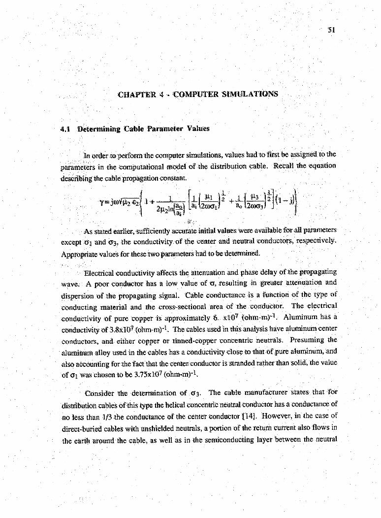
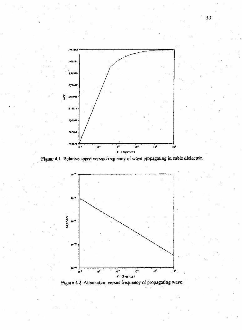
From this comparison it was found that within the given frequency range, a good match of the attenuation and phase delay results when the conductivity of the center conductor equals 3.75xl07 (ohm-m)"1, and the conductivity of the neutral conductor is five percent of a i, that is, 03 approximately equals 0.188xl07 (ohm-m)'1. Figure 4.1 shows the plot of v/c versus f and Figure 4.2 shows the plot of oc/f versus f, using these values of

(Ti and 03.

-

Figure 4 .1 Relative spged versus frequency of wave propagating in cable dielectric.

JL W t*

Figure 4.2 Attenuation versus frequency of propagating wave.

54

The above results provide initial parameter values for Oi and 63, and just as importantly, demonstrate that the proposed model for Y does, in fact, accurately describe

the cable propagation characteristics over the specified range of frequencies. Thus armed with all of the parameter values needed to calculate the cable propagation constant versus frequency, it is now possible to simulate the calibration experiments and compare the results against the experimental data to further develop the model of the distribution system.

Before performing the computer simulations, however, it is also possible to verify the accuracy of the proposed parameter values by utilizing the data from the tape-shielded cable experiment. The attenuation and phase delay values obtained from these measurements can be compared to the a and P determined from the computational model of

the cable propagation characteristics. For the tape-shielded cable, the Conductance of the copper neutral conductor is specified by the manufacturer as being approximately equal to the conductivity of the center conductor.

The center conductor of the tape-shielded cable is again stranded aluminum, thus 0 \ was set to 3.75xl07 (ohm-m)*1- Next, calculating a and P for various values of 03, it was

found that when 03 equals 9.5% of Oi the computed values compare well with the experimentally determined values, particularly at the higher frequencies (above I MHz). The measured values of a and P, previously listed in Table 3.1, are repeated here in Table 4.1, along with the calculated values of a and p computed at corresponding frequencies.

55

Table 4.1 Measured versus calculated values of attenuation and phase delay constants.

no.frequency

(MHz)

Measured alpha

(x 10-3)

Calculated alpha

ix 10*3)Measured

betaCalculated

beta

0.1 0.1162 0.1384 0.00369 0.00377

ru2 ; 0.2 &1476 0.1957 0.00724 0.00745

0.3 0.0954 0.2397 0.01104 0.01113

4 . 0.4 0.1144 0.2767 0.01453 0.01479

5 /; 0.5 0.2853 0.3094 0.01830 0.01846

6 0.6 0.1507 0.3389 0.02176 0.02211

7 ; 0.7 0.4264 0.3361 0.02547 0.02577

% 0.8 0.3326 0.3914 0.02921 0.02943

9 0.9 0.4945 0.4151 OJ03276 0.03308

10 1.0 ■ 0.4760 0.4376 0.03641 0.03673

11 2.0 0.6283 * 0.6188 0.07208 0.07320

12 V; 3.0 0.7567 0.7579 0.10794 0.10964

13 4.0 0.8106 0.8752 0.14394 0.14605

14 5.0 0.9354 0.9785 0.17987 0.18244

15 6.0 1.0589 1.0718 0.21585 0.21883

16 7.0 1.2383 1.1577 0.25160 0.25521

17 8.0 1.3759 1.2377 0.28729 0.29158

18 9.0 1.3616 1.3127 0.32329 0.32795

19 10.0 1.5460 1.3837 0.35903 0.36431

4.2 Calibration Measurement Simulations

iGiven A e cable parameters, it is now possible to implement the computational model and simulate Ae calibration and fault experiments. The computer program used to perform Ae following simulations was written by Al Englemann, a former Purdue graduate student, and Dr. Steiner. A few slight modifications were made to the program to make it suitable for use in this analysis. A listing of Ae simulation program can be found in the

Appendix.

The first step is to simulate the phase delay and attenuation experienced by the calibration pulse as it propagates in the cable. Working with the 723 foot section of distribution cable, the simulation parameters are specified and a IV calibration pulse is “injected” into the terminal end of the cable. The opposite end of the cable is left as an open circuit (although in the buried system the first transformer is connected to the far end of this cable). The calibration signal propagates from the terminal end to the open where it is reflected back to the input. The anticipated two-way transit time is approximately 2.9ps, as

this was the round-trip time between the terminal end and the first transformer measured in the system calibration experiment. (See Figure 3.7 for the system calibration waveform.)

The phase delay experienced by the propagating signal can be adjusted by varying £2, the permittivity of the cable dielectric. The actual permittivity of the dielectric is approximately 2.7eo, but this parameter value had to be increased to 4.0£o before the

simulated delay adequately matched the experimental delay. The primary effects of a higher permittivity are a lower velocity of propagation and an increased attenuation. Increasing £2

can be justified as a means to compensate for the longer distance the signal travels because the; concentric neutrals are wound around the insulation in a helical fashion, instead of

running straight along the length of the cable.

As previously indicated, three of the cables in the buried distribution system have six helically-wrapped wires in the neutral conductor and the other cable has eight. The pulse bounce program does not allow each distribution cable to be specified in terms of its own parameters, so the length of the cable with two extra wires was normalized (reduced) to account for a higher value of conductance. The normalization was based on measurements (taken by Dr. Steiner prior to this analysis) of the propagation delay (1/v) of

the two types of cables. It was known from the earlier measurements that the propagation delay of the cable with eight neutral wires was 96% of the propagation delay of the cables with six neutral wires. Hence, the length of the cable was reduced to 96% of its measured length (694 ft. = 723 x 0.96). The remaining parameter values of the four cables were then assumed to be identical. Table 4.2 lists the cable parameter values used in the simulations.

Table 4.2 Cable parameter values used in simulations.

Parameter Value .. Unit

Ol 3.75 x 107 (ohm-m)-l

. ; . ■ 03 5% CTl (ohm-m)-l

£0 8.85 X 10-12 ; ' F/m

V ; . ' . . 62 4.0 60 F/m

;i: ■■ ■■ W) 4jt x 10-7 H/to

■■■■'' P l MO B to

P2 MO B to

P3 MO H/m0.011218 m .

. aj 0.004808 m

. . ' • ■ :*fe . . . ■. ■ : W . ,

Once the propagation velocity of the distribution cables was correctly adjusted, the three other distribution cables, the section of faulted cable, ,and the transformers were added to match the configuration of the buried distribution system. The next stage of the simulations was to develop accurate representations for the transformers and fault so that the reflections caused by the discontinuities had shapes and amplitudes similar to the reflections seen in the experimental calibration waveforms (see Figures 3.6-9). In essence, this required finding the eormettchaiacteristicimpedance o f each component in the system. The options were to model the system components either as shunt admittances or as short sections of distribution cable with appropriate numerical values.

Since the reflections from the transformers are known to have a positive peak followed by a negative peak, the transformers must have a higher value of impedance than the distribution cable. After experimenting with various admittances and series sections of cable, it was determined that the simplest and most accurate transformer model was a short section (6 ft.) of series cable with a characteristic impedance of 50Q. A value of 50Q for the transformer characteristic impedance, along with 40Q for the characteristic impedance

of the cable, gives a reflection coefficient (looking into the transformer) of approximately 0.11. This value for T produces reflections of the correct polarity and magnitude. This can

be seen in Figure 4.3, which shows an expanded view of the simulated reflection from the

first transformer.

The system calibration waveforms indicate that the reflection from the fault site has a small negative peak, followed by a slightly larger positive peak, followed by another negative peak. To characterize the impedance discontinuity responsible for this reflection a three foot section of 35S2 cable in series with another three foot section of 50Q cable was

connected into the distribution system model at the fault location. The resulting reflection of the calibration signal is illustrated in Figure 4.4, where the amplitude as well as the position of the reflections match the experimental data.

The distribution transformers in the buried system are configured so that the current merely feeds through the transformer, with no connections to the secondary taps. Therefore, describing the transformer as a series section of distribution cable with a unique characteristic impedance seems a logical way to model the transformer. The short section of faulted cable has two features which are primarily responsible for the reflections it causes. First, the type of distribution cable is actually different from the other distribution cables in the system. That is, the materials and dimensions Used in its construction are not identical to those of the adjacent cables. Thus the cable has a different characteristic impedance. Second, the section of faulted cable is held in place by an apparatus which effectively splices the cables together. These splices result in an added capacitance between the center and neutral conductors, reducing the impedance at the each end of the faulted cable. These features produce reflections as seen in Figure 4.4.

Based on the models developed for the distribution cables, transformers and fault site, the calibration experiment was simulated and the resulting waveform is shown in Figure 4.5. The incident calibration pulse occurs at time zero and has an amplitude approximately equal to one. The peaks from left to right locate the first transformer, the fault site, the second transformer and the open circuit. (Refer to Figure 3.5 to See the corresponding circuit diagram.) Compare this simulated waveform to the measured calibration waveform of Figure 3.6. Notice especially the amplitudes, shapes and positions o f the reflections.

Another way to verify the model of the distribution network is to simulate the fault calibration experiment and compare the results to the measured waveform. Initiating the calibration signal at the fault site and observing the waveform from the terminal end of the

59

system (see Figure 3.10), the simulated waveform replicates the outcome of a similar experiment performed on the buried system. Figure 4.6 shows the simulated fault calibration waveform and Figures 3.11 and 3.12 show the experimental results. The tallest peaks indicate the calibration pulse reflecting back and forth between the fault site and the detector with a delay of approximately 5.3ps. In addition to providing the transit time

between the fault site and the terminal end of the cable, the simulated waveform is also useful for determining the location of the reflections from the transformer. As mentioned in the previous chapter, the transformer reflections appear approximately 2.4 and 2.9ps after

the arrival of the incident calibration pulse.

~ '#<* T 3 6 3 M t . t i t t l t.OWIB 0.7M 00 »0*30* 3 .0 e m 0.1000» 3 . *9363 3 .1 MT*

t l M < * * C ) < X 1 0 " 6 >

Figure 4.3 Expanded view of simulated reflection from first transformer,

^ .170004

JV* — — :— r—-------I-------------- 1------------ r----------- 1------------1------------ r— II . «339« 9.96691 9.69989 9 .« tt7T 9.8697« 9.99864 9.63199 9.76998 9.99796

t lo w f < a * c > < X 10- 6 >

Figure 4.4 Expanded view of simulated reflection from fault site.

61

i.«mi

-.035441OfllOOO .137314 .37473(1 .113033 '.»».«44 .646431 ,034137 .361864 1.03093

i t * * < s#c> <xi<rs>Figure 4.5 Simulated system calibration measurement

^000000 .18713H .37H868 .S61H0I .7H9033 .938649 1.12360 1.3099H 1.99707

t im e < sec> <X10"5 >

Figure 4.6 Simulated fault calibration measurement.

62

4.3 Fault Measurement Simulations

The Hnal measurements obtained from the buried distribution system were the fault transient waveforms as observed from both the terminal and open circuit ends of the system. For these measurements, the thumper was used to energize the cable and break down the dielectric at the fault.

The pulse bounce program is not equipped to simulate the breakdown of the fault on a cable system. The program can simulate the calibration waveforms using an impulse function; however, simulating a line fault requires the application of a step change in voltage at the fault site. Unfortunately, a step input was not a feature available in the pulse

bounce program.

Still, it is possible to construct the fault measurement waveforms in either of the following two ways. First, a graphical pulse bounce diagram can be used to determine the time delays and relative amplitudes of the reflections found in the fault waveform. By using a voltage step for the input signal, the response of the distribution system reproduces the fault waveform. Another way to construct the fault waveform is to integrate the impulse response (i.e., the simulated fault waveform) to obtain the step response. These two methods will be demonstrated shortly.

The first fault measurement performed on the distribution system involved observing the fault event from the terminal end of the system with the normal detector. (See Figure 3.14 for the circuit diagram and Figures 3.15 and 3.16 for the measured waveforms.) This experiment was simulated by placing a low-value shunt impedance at the fault site in order to represent the arcing fault. The terminal end of the system was left as an open circuit (even though the thumper circuit actually appears like a lower impedance to the high frequency components of the transient signal). The model of the transformer was unchanged.

Figure 4.7 shows the simulated fault transient as detected from the terminal end of the system. The two-way time delay between the fault arid the detector is approximately 5.3ps, as was also determined from the fault measurement of Figure 3.16. The smaller

peaks are due to reflections at the transformer which is located between the fault and the terminal. As expected, these smaller peaks occur approximately 2.3 and 2.9)j.s after the

first pulse. (The fault measurement Of Figure 3.16 also indicated small peaks around this

time, although the measured waveform has been filtered significantly and the peaks are difficult to identify precisely.)

iThe first reflection from the transformer, seen in Figure 4.7, represents the time required for the fault transient to travel from the fault site to the transformer, where it is reflected back to the fault, inverted and reflected again back to the transformer where it is then transmitted through to the detector. This represents a total distance of 2395 ft. o f distribution cable and one pass through the transformer. The second peak from the transformer indicates the time required for the fault transient to travel from the fault site through the transformer to the detector, back to the transformer and then back to the detector, for a total distance of 2649 ft. of cable and one trip through the transformer. Other reflections also occur between the various impedance discontinuities in the system

bnt are too small to be detected.

The waveform of Figure 4.7 is the simulated impulse response of the faulted system. The actual fault waveforms result from a step input from the thumper. The integral of an impulse function is a step function, therefore, the step response of the distribution system can be obtained by integrating the impulse response. This integration can be performed by expanding the time scale around the peaks seen in Figure 4.7 to determine the area under the pulses. The area is then plotted against time and the resulting waveform represents the actual fault waveform. This integration was performed on the waveform of Figure 4.7 and the results are shown in Figure 4.8. The waveform of Figure 4.8(a) does not account for the effect the RC detection network has on the waveform. To improve the accuracy of the waveform, the 5jis RC time constant of the detector is

considered and the resulting waveform is shown in Figure 4.8(b). In terms of timing and waveshape, this transient wave now clearly resembles the actual fault measurement of Figure 3.16.

64

-O .663321

OOOOOO . 167316 .37H633 .861983 .7^9870 .936866 1.12391 1 .3 u e S 1.99699

t i m e < s e c > CXIO"®)

5

Figure 4.7 Simulated fault measurement from terminal end of system.

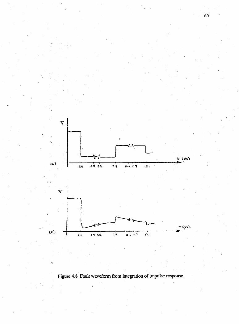
\o . \ VO.T

Figure 4.8 Fault waveform from integration of impulse response.

66

The final fault measurements were taken from the open circuit end of the system with the resistive detector, as seen in Figures 3.18 and 3.19. This experiment was simulated by placing a low value shunt impedance at the fault site, leaving the transformer in place and representing the resistive detector as a high impedance. (See Figure 3.17 for the circuit diagram.) The resulting simulation waveform is shown in Figures 4.9 and 4.10. Note the reflections between the fault and the open circuit, as well as reflections from the transformer.

As seen from Figure 4.9, the round-trip travel time between the fault and the open circuit is approximately 5.6|is, compared to the measured time of approximately 5.7(is.

The simulated waveform also shows that the first two reflections from the transformer are expected to occur around 1.9 and 3.8|is after the fault transient arrives at the detector. This

result was confirmed in the previous chapter, where it was noted that the fault measurement of Figure 3.19 does have small peaks in these positions.

The circuit diagram representing the fault measurement from the open circuit end of the system is shown in Figure 4.11 and the corresponding pulse bounce diagram appears in Figure 4.12. The time delays experienced by the transient signal propagating in the distribution system were determined from the system calibration waveform. The amplitude (A) of each reflection is shown to the left of the appropriate time delay. The amplitudes given here were calculated based upon the reflection coefficients for the system impedance discontinuities. The attenuation due to the cable propagation characteristics was not included. Other simplifications to the pulse bounce diagram include the omission of minor reflections and the assumption that the reflection coefficients and propagation delays are

constant for all frequencies.

The amplitude and phase delay information obtained from the graphical pulse bounce diagram was used to construct the fault waveforms of Figure 4.13. The waveform of Figure 4.13(a) illustrates the timing and amplitude characteristics, but does not account for the rise time (sloped edges) of the faulting transient. When this rise time is approximated and minor reflections from the transformer are added, a more accurate picture of the fault transient is obtained, as seen in Figure 4 .13(b). Compare this waveform to the fault measurements of Figures 3.18 and 3.19. Note the similarities between the measured and graphical fault transients in terms of timing and general waveshape.

Figure 4.11 Circuit diagram for fault measurement from open circuit end of system.

4.70|is (transformer)

10.39ps (transformer)

14.21ns (fault)

Figure 4.12. Bounce diagram for fault measurement from open circuit.

68

< 4 8 S 10.4- » a .l 14.3.z.e 4H

8.S 10.4- 11.3 V4.1.

Figure 4.13 Fault waveforms from pulse bounce analysis.

69

4.4 Pulse. Bounce Simulation Program

Comments have already- been made regarding a few of the. limitations of the pulse bounce'program. For instance, it is not, possible to* specify each cable in the distribution system according to its own unique parameters,, nor can. the program simulate the system step response needfed to represent the aetuaifault waveforms

There are two other points: that need to be mentioned regarding the results of the computer simulations. First, the program? uses an impulse function as the: stimulus to the distribution system, under evaluation. An. impulsive input generates reflections from the impedance' discontinuities which are* extremely narrow, as can be seen? in any of the simulated waveforms. Because the reflections are so narrow, the peak amplitudes being Computedf tend to be heavily dependent, on? the simulation- interval* and the? number of samples within the interval.. If the. sampling rate:is too-low, the-amplitudes in the. resulting waveform may be much lower than they should be. (This- could significantly affect the outcome of an integration1 of the impulse response.): Thereforevit is-advisable that several? simulations be: performed for each system: configuration, using various simulation parameters. Then carefully evaluate the waveform to ensure it seems logical and appears correct;.

One final note. There are slight’numerical instability problems seen in some of the simulated- waveforms; In particular; Figure 4.4' shows the simulated reflection from the fault site:.. OteeiMer sidte o f this; reflection there are: several; microseconds of oscillations. These oscillations are actually due to numerical, problems encountered during the calculations and are not aphenomenon seen in the actual* measurement; The magnitude of the numerical instability is,also,dependent on Me simulation parameters.

CHAPTER 5 - SUMMARY AND RESULTS

5.1 Analysis of the Proposed Computational Model

The objective of the preceding analysis was to develop and assess the computational model proposed to describe the propagation characteristics of fault transients in underground residential distribution cables. The proposed model was derived from an approximation for the propagation constant of coaxial cables. The equation and associated parameter values were modified in an effort to represent a single phase concentric neutral distribution cable.

M easurem entsweremadeonprimarydistributioncabletoacquireattenuationand phase delay data for signals propagating in the cable. Next, experiments were performed on the buried distribution system to get system calibration and fault transient waveforms. The experimental results were then used to determine the appropriate parameter values in the cable model and to develop a theoretical representation of the entire cable system; including cables, transformers, line faults, and cable terminations.

Ohce the total system model was accurately defined, computer simulations were performed to generate system calibration and fault measurements. The simulated waveforms were then compared to the actual calibration and fault waveforms taken on theburied system.

The criteria used to evaluate the computational model included the accuracy of the calculated propagation characteristics and the applicability of the model to the study of fault transients The results are as follows: •

• Over a limited frequency range (approximately IOkHz to 10MHz) the computational model of the cable propagation characteristics can accurately describe the attenuation and phase delay experienced by transients propagating in concentric neutral distribution cables.

71

While producing adequate results, the cable model is relatively simple and easy to evaluate, making it well-suited for computer implementation.

A computer program, based on the computational model, can be used to simulate a multi-component distribution system consisting of a fault and one or more distribution cables, transformers, and/or cable terminations. The computersimulations can generate system calibration or fault transient waveforms.

The simulated waveforms are useful for studying fault transient behavior in general, or for identifying the location of specific system discontinuities.

U ST OF REFERENCES

LIST OF REFERENCES

flj IEEE Conference Record; 1976 Underground Transmission and D istribution Conference, IEEE Power Engineering Society, IEEE, Inc., New York, 1976.

[2] E. B. Kurtz and T. M. Shoemaker, The Lineman’s and C ablem ans Handbook, McGraw-Hill BookCo., New York, 1981,

[3] J. Tyner, "Underground distribution problems still abound", Transmission and Distribution, vol. 37, pp 20-28,1985 December.

[4] B. K. Hwang, "Latest developments in long-life cables: insulating, semi- conducting and jacketing materials", Wire Journal International, vol. 19, pp 58-64, 198b December.

[5] J. Alton, "Is the tide turning for x.l.p.e.?", Electrical Review , vol. 219, pp 32-3,1986 September.

[6] J. Lawson, "Picking the right URD cable isn't easy", Electrical W orld, vol. 40-1,1987 May.

[7] G. J. Conroy, "Cable Fault Locating by Electronic Means", M ine P o w er D istribution, ed. Bureau of Mines, Proceedings: Bureau of Mines TechnologyTransfer Seminar Pittsburgh, PA, pp 104-114, Washington, DC, 1975 March.

J i j D. Fielding, "Mastering the HV impulse method of finding faults in bpried cables”. Electricity Canada, vol. 34, pp 8-20,1984 February.

[9] R. W. Deltenre, J. J. Schwarz, H, J. Wagnon, "Underground Cable Fault Location", EPRI E l-363, R esearch P ro jec t 481-1 , Electric Power Research Institute, Palo Alto, CA, 1977 January.

[10] IEEE Transactions on Pow er D elivery, IEEE Power Engineering Society, vol. 4, no. 2, IEEE, Inc., New York, 1989 April.

[11] W. L. Weeks, Electromagnetic Theory For Rnginemng Applications, Jrifeh Wiley and Sons, Inc,, New York, 1964.

[12] W. L, Weeks, Transmission and Distribution o f E lectrical Energy, Harper and Row, New York, 1981.

[13] L. C. Shen and J. A. Kong, A pp lied E lectrom agnetism , PWS Engineering, Boston, MA, 1987.

[14]

[15]

Essex, Underground Cable Engineering Handbook, United Technologies, Essex Group, Marion, IN, 1980.

Y. Diao, Propagation o f W ide Band Signals in P ow er C ables, Ph.D. Thesis, Purdue University, 1984.

AdHitional References

T. Tanaka and A. Greenwood, Advanced Pow er Cable Technology, CRG Press Ine., Bdca Raton, Florida, 1983.

A. J. Pansini, Under grounding E lectric Lines, Hayden Book Company, Inc., Rochelle Park, New Jersey, 1978.

\ APPENDIX

This appendix contains the computer program, called pbnce 6, which generates a rough approximation to the impulse response of a cable system with multiple discontinuities. It permits information concerning the variation of propagation characteristic with frequency to be included. The program itself is a result, primarily, of the joint efforts of Alan J. Englemann and Dr. James P. Steiner.

CCCG0C '•gGCGCGe

■ c '■

GGGGGGd .'G

■ G 'dG .GGdG

■ G - .CG'GCGG ■ G G C G £GG

. C G C G G Gc-'C G GS G '; G-:'' C ' :CGGGGG<?G

. ' p r o g r a m p b n c e 6

P R O G F t A M D E S C R I P T I O N :G i v e n a s y s t e m m o d e l e d a s a s e t o f c o a x i a l c a b l e s h a v i n g s p e c i f i e d d i m e n s i o n s , p e r m i t t i v i t y , p e r m e a b i l i t y , a n d c o n d u c t i v i t y , a n d f r e q u e n c y d e p e n d e n t , s e c o n d o r d e r s h u n t a d m i t t a n c e s

g r o u n d , p b n c e 6 w i l l c a l c u l a t e t h e t i m e d o m a i n t r a n s i e n t • • •- ' # a f t ? e £ 6 r n v . a p p e a r i n g a t a g i v e h o b s e r v a t i o n p o i n t i n t h e s y s t e r r i

a s r e s u l t i n g f r o m a u n i t i m p u l s e i n j e c t e d a t a s p e c i f i e d p o i n t i n t h e s y s t e m . P b n c e e p e r f o r m s a b o u n c e a n a l y s i s a t a h U r n b d r o f f r # q u d h e i # s t o o b t a i n I i f G q u e n c y d o m a i n R e p r e s e n t a t i o n o f r G s i i i t a n t w a v e f o t m , w h l G h i s t h e n t r a n s f o r m e d i n t o t h e t i m e ( f o i M i h b y u s e o f a n F F T . P r o p a g a t o n c h a r a c t e r i s t i c s a r e f r e q u e n c y d e p e n d e n t a n d c a l c u l a t e d f r o m t h e s p e c i f i e d c a b l e p a r a m e t e r s u s i n g a G G f f i p U R a t i o n a l m o d d i o f t h e c a b l e p r o p a g a t i o n c o n s t a n t b a s e d o n a n a p p r o x i m a t e f o r m u i a f o r G d a x i a l c a b l e s d e r i v e d i n W e e k s '

e I e c t r d r i i a g h e t i c s M d k , p . « 7 :

g a m n t a = b e t a * ( I .*Q + i 0 >/ (2 , 0 * m u 2 * a l o g ( a o / a i ) )I * ( s q r t ( m a i / ( 2 ; 0 * w * s i g l ) * l / a i f s q r t ( m u 3 / 2 , 0 * w * s i g 3 ) * 1 / a o ) )

I * d f f i p l x ( I i O / - 1 . 0 ) )

( p a r a m e t e r s a r e d e f i n e d i n t h e f o l l o w i n g p r o g r a m ) . A n a l y s i s i s c o n s t r a i n e d b y a m a x i m u m t i f f i d c o n s t r a i n t a n d m i n i m u m a m p l i t u d e c o n s t r a i n t . N t u f i b e R o f p o i n t s a p p e a r i n g i n r e s u l t i s a u s e R s p e c i f i e d , i n t e g e r p o w e r o f t w o .

I N P U T : r t i f l 6 " , s y n t a x d e s c r i b e d b e l o wO U T P U T : " d u t e " , a m p l i t u d e o f r e s u l t a n t w a v e f o r m .

rt t i m G 6 M , t i m e i n f o r m a t i o n c o r r e s p o n d i n g ; - i d " d i l t # " y d a t a

I N P U T F O R M A T :a . l i n e p a r a m e t e r s - e a c h l i n e d e f i n e d i n t e r m s o f : t w o b o u n d a r i e s , -

e a c h i n d e x e d b y u n i q u e i n t e g e r s ; a c h a r a c t e r i s t i c i m p e d a n c e Z O ( r e a l ) ; a n d a c a b l e l e n g t h ( u n i t o f l e n g t h s h o u l d c o r r e s p o n d w i t h t h a t u s e d i n d e l a y p a r a m e t e r ) . N o t e t h a t t h e o r d e r i n w h i c h t h e b o u n d a r i e s a r e n u m b e r e d i s n o t i m p o r t a n t , h o w e v e r , f o r a n y s y s t e m d e f i n e d w i t h N b o u n d a r i e s , o n l y i n t e g e r s f r o m I t o N m a y b e U s e d , a s l i b n e m a y b e s k i p p e d . E a c h c a b l e m u s t b e d e f i n e d i n t h i s m a n n e r ; p a r a m e t e r s m u s t a p p e a r o n o n e l i n e i n t h e f o l l o w i n g s e q u e n c e : .

> b d f y i , b d r y 2 , Z 0 , l e n g t h

( e n d t h i s f i e l d w i t h a l i n e o f a l l z e r o d a t a )

b . c o n n e c t i o n d a t a - d e f i n e a l l b o u n d a r y - t o - b o u n d a r y c o n n e c t i o n s .I f t h e r e e x i s t s a h y n o d e a t w h i c h m o r e t h a n - t w o b o u n d a r i e s a r e c o n n e c t e d , t h e n a b o u n d a r y - t o - b o u n d a r y c o n n e c t i o n m u s t b e d e f i n e d f o r e v e r y p o s s i b l e b o u n d a r y p a i r i n t h e s e t ; e . g . i f b o u n d a r i e s a , b , c a r e c o n n e c t e d , t h e n c o n n e c t i o n s m u s t b e d e f i n e d f o r a - b , b - c , a n d c - a . C o n n e c t i o n s m u s t e a c h b e i n p u t i n t h e f o l l o w i n g m a n n e r :

> b d r y l , b d r y 2

( e n d w i t h z e r o s )

C . l u m p e d a d m i t t a n c e s a n d t e r m i n a t i o n s - i n p u t c o m p l e x a d m i t t a n c e s W h i c h a T e t o a p p e a r a s s h u n t e l e m e h t s t o g r o u n d i n t h e s y s t e m .

/ ' t h e s e a r e t o b e d e f i n e d i n t e r m s o f c o m p l e x c o e f f i c i e n t s o f t h e

f o l l o w i n g p o l y n o m i a l e x p r e s s i o n :

Y ( W )

a O + a L * w + a 2 * w * ‘ 2

c b O + b l * w + b 2 * w * * 2Ccc F o r s h u n t e l e m e n t s a p p e a r i n g a t c o n n e c t i o n s o f t w o o r m o r ec b o u n d a r i e s , t h e a d m i t t a n c e m u s t b e d e f i n e d a t o n l y o n ec o f t h e b o u n d a r i e s i n v o l v e d . O n l y o n e s h u n t e l e m e n t m a y b ec d e f i n e d a t e a c h n o d e . C a r e m u s t b e t a k e n t h a t t h e d e n o m i n a t o rc d o e s n o t b e c o m e z e r o a t w - 0 , i . e . b O m u s t a l w a y s b e n o n - z e r o ,c I f n o a d m i t t a n c e i s s p e c i f i e d a t a n o d e , i t i s a s s u m e d t o b ec z e r o ( i n f i n i t e i m p e d a n c e ) , D a t a i s e n t e r e d a s f o l l o w s :cc > b d r y , a O , a l , a 2 , b O , b l , b 2c ■c ( e n d w i t h z e r o s )cc d . s i m u l a t i o n p a r a m e t e r s - D e f i n e t h e b o u n d a r y a t w h i c h t h e s y s t e m c w i l l b e o b s e r v e d , a n d t h e b o u n d a r y a t w h i c h t h e s i g n a l i s t oc o r i g i n a t e . A n a l y s i s i s c o n s t r a i n t e d b y a s t o p t i m e a n d ac m i n i m u m s i g n a l m a g n i t u d e . T h e s i g n a l b e g i n s a t t i m e =» 0 , a tc a n a m p l i t u d e o f o n e . S u b s e q u e n t r e f l e c t i o n s a r e f o l l o w e d u n t i lc t h e s t o p t i m e i s e x c e e d e d o r t h e m a g n i t u d e o f t h e s i g n a l f a l l sc b e l o w t h e s p e c i f i e d l i m i t . N u m b e r o f p o i n t s u s e d i n t h e a n a l y s i sc m u s t a l s o b e g i v e n , a n d i t s c o r r e s p o n d i n g b a s e 2 l o g a r i t h m ,c S i n c e t h e F F T i s i n v o l v e d , t h e n u m b e r o f p o i n t s m u s t b e a n i n t e g e rc p o w e r o f t w o . S a m p l i n g t i m e a r i d b a n d w i d t h w i l l b e b a s e d o n t h ec n u m b e r o f a n a l y s i s p o i n t s , a n d t h e s p e c i f i e d t i m e i n t e r v a l ,c A n a l y s i s p a r a m e t e r s a r e i n p u t i n t h e f o l l o w i n g s e q u e n c e :cc > o b s e r v a t i o n b d r yc > b d r y w h e r e s i g n a l o r i g i n a t e sc > s t o p t i m e ( s e c o n d s )c > m i n i m u m s i g n a l m a g n i t u d e ( I i s m a x )c > n u m b e r o f p o i n t s N S , l o g b a s e t w o o f N S

cCc A l l l i n e i e n g h t h s a r e a s s u m e d t o b e - - * ^c s u c h t h a t t h e d r i v i n g p o i n t i m p e d a n c e o f a l i n e i s i t s c c h a r a c t e r i s t i c i m p e d a n c e , c cc E X A M P L E I N P U T F I L E : cC I 2 5 0 . 1 0 0 .c 3 4 7 0 . 1 0 0 .c 0 0 0 . 0 .c 2 3 ■c 0 0c I ( I . 0 , 0 . 0 ) ( 0 . , 0 . ) ( 0 . , 0 . ) ( 5 0 . , 0 . ) ( O ' . , 0 . ) ( 0 . , 0 . )

c 2 ( 1 . 0 e - 8 , 0 . 0 ) ( 0 . , I . e - 1 2 ) ( 0 . , 0 . ) ( 1 . 0 , 0 . ) ( 0 . , 0 . ) O O

c 4 ( I . 0 , 0 . 0 ) ( 0 . , 0 . ) ( 0 . , 0 . ) ( 5 0 , 0 . ) ( 0 . , 0 . ) ( 0 . > 0 . )

C O ( 0 . 0 , 0 . 0 ) ( 0 . , 0 . ) ( 0 . , 0 . ) ( 0 . , 0 . ) ( 0 . , 0 . ) ( 0 . , 0 . )

c Ic lc 1 0 e - 6 .c I e - 2 ' ■c 1 0 2 4 1 0CC ■ ' V.c V A R I A B L E S :Cc A ( I ) : s i g n a l a m p l i t u d e S T A C K .c a 0 , a l , a 2 : s h u n t a d m i t t a n c e n u m e r a t o r c o e f f i c i e n t s i n p u tc v a r i a b l e s .c a b u f ( i ) : s i g n a l a m p l i t u d e O U T P U T B U F F E R ,c a i n c : i n c i d e n t s i g n a l a m p l i t u d e v a r i a b l e .c .... a f ( i ) : a t t e n u a t i o n c o e f f i c i e n t P A R A M E T E R A R R A Y a t a s p e c i f i c

gCCCGCCCCCCGGGGCGGGGGCCGGCCGGCCCCCCCCCGCGCGGCCCCCGCCCCCCCCG

f r e q u e n c y , f o r e a c h c a b l e h a v i n g b o u n d a r y ( i ) . a m i n : m i n i m u m s i g n a l a m p l i t u d e c r i t e r i o n .B ( i ) : b o u n d a r y i n d e x n u m b e r S T A C K .b O , b l , b 2 : s h u n t a d m i t t a n c e d e n o m i n a t o r c o e f f i c i e n t s i n p u t

v a r i a b l e s .b e t a : b e t a p r o p a g a t i o n d e l a y p a r a m e t e r .c a b l e n ( i ) : c a b l e l e n g t h P A R A M E T E R A R R A Y , l e n g t h o f e a c h c a b l e

w i t h b o u n d a r y ( i ) .c i m p c h a r a c t e r i s t i c i m p e d a n c e i n p u t v a r i a b l e , c j : u n i t i m a g i n a r y q u a n t i t y .c o e f ( i ) : a r r a y u s e d t o p a s s p o l y n o m i a l e x p r e s s i o n c o e f f i c i e n t s

t o s u b r o u t i n e .c s u m : c o m p l e x s u m a c c u m u l a t o r .c y p : c o m p l e x a d m i t t a n c e v a r i a b l e .c z p : c o m p l e x i m p e d a n c e v a r i a b l e .d e l t a f : f r e q u e n c y i n c r e m e n t o f a n a l y s i s .d e l t a t : s a m p l i n g i n t e r v a l i n r e s u l t a n t w a v e f o r m .d l e n : c a b l e l e n g t h i n p u t v a r i a b l e .g a m m a : p r a p a g a t i o n c h a r a c t e r i s t i c p a r a m e t e r .i b l , i b 2 : b o u n d a r y i n d e x n u m b e r i n p u t v a r i a b l e s .i b o b s : o b s e r v a t i o n b o u n d a r y i n d e x n u m b e r .i b s o r : i n d e x n u m b e r o f b o u n d a r y a t w h i c h s i g n a l o r i g i n a t e s , i b u f : i n d e x f o r O U T P U T B U F F E R S . . _i s l , i s 2 : b o u n d a r y i n d e x n u m b e r p a r a m e t e r s , " s i d e O n e r a n d

" s i d e t w o " .i s n 2 : l o g b a s e 2 o f N S . .i t e r b : m a x n u m b e r o f n e w s i g n a l s g e n e r a t e d b y a n y o n e s i g n a l .I T Q S i i n d e x f o r S T A C K S , t o p o f s t a c k i n d i c a t o r , k : s t a c k p o i n t e r i n d e x . Vs\M ( i , j ) : C O N N E C T I O N M A T R I X , i n d e x e d b y b o u n d a r y n u m b e r s :

M ( i , j ) = I : i c o n n e c t e d t o jM ( i , j ) = - I ; i a n d j a t o p p o s i t e e n d o f s a m e c a b l e M ( i , i ) =■ I : i i s t h e o b s e r v a t i o n p o i n t M ( i , j ) =- 0 : o t h e r w i s e

N : t o t a l n u m b e r o f b o u n d a r i e s i n t h e d e f i n e d s y s t e m .N F R E Q : f r e q u e n c y c o u n t e r .N M A X : m a x i m u m n u m b e r o f b o u n d a r i e s i n s y s t e m .N S : n u m b e r o f p o i n t s i n r e s u l t a n t w a v e f o r m .N S T A C K : m a x i m u m s t a c k s i z e .P I : m a t h e m a t i c a l c o n s t a n t p i . . nr h o ( i ) : r e f e c t i o n c o e f f i c i e n t P A R A M E T E R A R R A Y , r e f l e c t i o n

c o e f f i c i e n t l o o k i n g o u t o f c a b l e a t c a b l e e n d d e f i n e d b y b o u n d a r y ( i ) , a t a s p e c i f i c f r e q u e n c y ,

s c f ( i / j ) : ( j ) t h c o e f f i c i e n t s d e s c r i b i n g p o l y n o m i a l e x p r e s s i o n s f o r s h u n t a d m i t t a n c e s c o n n e c t e d t o b o u n d a r y ( i ) ( P A R A M E T E R A R R A Y S ) .

t ( i ) : s i g n a l t i m e d a t a S T A C K .t a u ( i ) : d e l a y P A R A M E T E R A R R A Y , t i m e d e l a y o f c a b l e h a v i n g

b o u n d a r y ( i ) , a t a s p e c i f i c f r e q u e n c y . t b u f ( i ) *. s i g n a l t i m e d a t a O U T P U T B U F F E R , t m a x : m a x i m u m t i m e c r i t e r i o n .w : r a d i a n f r e q e n c y . . .X ( i ) : v e c t o r i n w h i c h i s d e p o s i t e d f r e q u e n c y d o m a i n r e s u l t s

a t e a c h f r e q u e n c y i n c r e m e n t . E v e n t u a l l y c o n t a i n s f r e q d o m a i n r e p r e s e n t a t i o n o f r e s u l t , a n d i s i n v e r s e t r a n s f o r m e d

i n t o t i m e d o m a i n .Z c h a r ( i ) : c h a r a c t e r i s t i c i m p e d a n c e P A R A M E T E R A R R A Y , c h a r

i m p e d a n c e o f c a b l e h a v i n g b o u n d a r y ( i ) .

E R R O R M E S S A G E S :

l i n e l i m i t e x c e e d e d : s y s t e m h a s t o o m a n y l i n e s ; , i n c r e a s e N M A X . b o u n d a r y c o n n e c t e d t o i t s e l f : c o n n e c t i o n d a t a e r r o r , s e l f

e x p l a n a t o r y .

e x c e s s c o n n e c t i o n d a t a

c w h a t i s p o s s i b l e .o . z e r o i m p e d a n c e t o g r o u n d : s h u n t i m p e d a n c e h a s b e e n d e f i n e d a sc z e r o - t h i s i s n o t a l l o w e d ,c t o p m a n y l u m p e d i m p e d a n c e s : m o r e s h u n t i m p e d a n c e s d e f i n e d t h a nc w h a t i s p o s s i b l e .c o n e s i d e d c a b l e : n o o p p o s i t e s i d e d e f i n e d i n c o n n e c t i o n m a t r i x ,c e x c e e d e d s t a c k s i z e : N S T A C K e x c e e d e d - e i t h e r i n c r e a s e t h i sc p a r a m e t e r o r c h a n g e a n a l y s i s p a r a m e t e r sc t o d e c r e a s e n u m b e r o f s i g n a l s c a l c u l a t e d ,c E X C E E D E D n n n I T E R A T I O N S F O R S I G N A L : o n e s i g n a l h a s p r o d u c e dc e x c e s s i v e n e w s i g n a l s ,c C h a n g e i t e r b v a l u e o rc a n a l y s i s p a r a m e t e r s ,c E X C E E D E D n n n I T E R A T I O N S O N S T A C K : s t a c k s i z e e x c e e d e d . S e e a b o v ec b O i s z e r o f o r s h u n t a d m i t t a n c e : b O c o e f f i c i e n t d e f i n e d f o r ac s h u n t a d m i t t a n c e t e r m i s z e r o ;c c h a n g e t o n o n - z e r o v a l u e ,c ■ _ > .

c ■ .C a . e n g e l m a n n , 1 9 8 8 c u p d a t e d 1 2 - 1 6 - 8 8 c u p d a t e d 6 ^ 1 5 - 8 J ( I i u r )c :

p a r a m e t e r ( N M A X - 2 0 / N S T A C K - 2 5 0 0 0 / N S M A X = 8 1 9 2 )c . . in teger 13 (NSTACK), M (NMAX, NMAX)

c o m p l e x r h o ( N M A X ) , z c h a r ( N M A X ) , A ( N S T A C K ) , a b u f ( N S T A C K ) c o m p l e x X ( N S M A X ) , s c f ( N M A X , 6 ) , c o e f ( 6 ) , g a m m a , b e t a c o m p l e x c a d m , c y p , c z p , a i n c , c s u m , c j , a O , a l , a 2 , b O , b l , b 2 r e a l c a b l e n ( N M A X ) , t ( N S T A C K ) , t a u ( M M A X ) r e a l a f ( N M A X ) , t b u f ( N S T A C K ) , m u l , m u 2

c ' ■ ' • ' V \ v ..•.■■■■ •' . ■. ■ . :c

open( I, File=3nOUte") open(2,file=nin6n)

c ppen( 3/f He=anS tack6 " )Ppen(IHile=l̂ imeen)

c \ f- k k h -f t + T f+-H-H- + f- F f- +h h h h H - H H f f t H c I. INPUT AND INITIALIZATIONSC + f f l - :h l + + + l l l - + + + + + + + + f f + + + + f 4- + + + + f + + + + H +

c c o n s t a n t s :P1=4.O *ATAN(1.0) ; c j = ( 0 . 0 / 1 . 0 )

Cccccccccc

t f * f a c t o r f o r a d j u s t i n g t i m e d e l a y e p s r = r e i a t i v e p e r m i t i v i t y o f d i e l e c t r i c e p s C N p e r m i t i v i t y o f f r e e s p a c e e p s 2 = r e a l p e r m i t t i v i t y o f d i e l e c t r i ce p s 2 t = r e a l p e r m i t t i v i t y o f d i e l e c t r i c , w i t h t i m e d e l a y a d j u s t m e n tS L g l = C o n d u c t l v i t y o f c e n t e r c o n d u c t o rs i g 3 “ c o n d u c t i v i t y o f o u t e r n e u t r a l c o n d u c t o r sm u l = m u 3 = p e r m e a b i l i t y o f c o n d u c t o ra i , a o = i n n e r a n d o u t e r r a d i u s o f d i e l e c t r i c

s e t c a b l e p a r a m e t e r st f = 3 . 0e p s r = 2 . 7e p s 0 = 8 . 8 5 e - 1 2e p s 2 = e p s r * e p s Qe p s 2 t = ( t f / e p s r ) * e p s 2m u 1 = 4 . 0 * P I * 1 . O e - 7m u 2 = m u li n u 3 = m u ls i g l = 3 . 7 5 e 7

O O

s i g 3 - 0 . 0 5 * s i g l a i - O . 0 0 9 6 1 5 / 2 . 0 a o ~ 0 . 0 2 2 4 3 6 / 2 . 0 z c h a r - 4 0 .

c A . I n i t i a l i z e c o n n e c t i o n m a t r i x , s t a c k , a n d c o < d o 1 0 5 1 = 1 , N M A X s c f ( i , I ) = ( 0 . 0 , 0 . 0 ) s c f ( i , 2 ) = ( 0 . 0 , 0 . 0 ) s c f ( i , 3 ) ^ ( 0 . 0 , 0 . 0 ) s c f ( i , 4 ) - ( l . 0 , 0 . 0 ) s e f ( L , 5 ) » ( 0 . 0 , 0 . 0 )

s c f ( i , 6 ) = ( 0 . 0 , 0 . 0 ) d o 1 0 5 j = l , N M A X M ( i , j ) = 0

1 0 5 c o n t i n u e

> e f f i c i e n t a r r a y s

1 0 6

d o 1 0 6 i = I , N S T A C KB ( i ) = 0c o n t i n u e

c B . I n p u t s y s t e m p a r a m e t e r s , c o n s t r u c t m a t r i c e s

c — , ' . , ■ .c r e a d c a b l e d a t a ( a t m o s t N M A X / 2 )

d o H O k o u n t = I , N M A X / 2 r e a d ( 2 , * ) i b l , i b 2 , c i m p , d l e n

c c o n v e r t c a b l e l e n g t h f r o m f e e t t o m e t e r s d i e n = d l e n * . 3 0 7 7 ^i f ( i b l . E Q . 0 ) g o t o 1 2 0 f

c f i l l i n " o p p o s i t e e n d " i n d i c a t o r s i n c o n n e c t i o n m a t r i x M ( i b l , i b 2 ) = - l M ( i b 2 , i b l ) = - 1

G p u t r e a l c h a r i m p e d a n c e i n t o c o m p l e x p a r a m e t e r a r r a y z c h a r ( i b i ) = c m p l x ( c i m p , 0 . 0 ) z c h a r ( i b 2 ) = C m p l x ( c i m p , 0 . 0 )

c a b l e n ( i b l ) = d l e nC a b l e n ( i b 2 ) = d l e n .

c v a r i a b l e N k e e p s t r a c k o f h o w m a n y b o u n d a r i e s a r e i n t h e s y s t e m

N = k o u n tH O c o n t i n u e c e r r o r i f N M A X e x c e e d e d

S T O P " l i n e l i m i t e x c e e d e d "

c r e a d c o n n e c t i o n d a t a ( M h a s o n l y N M A X / 2 * N M A X / 2 e l e m e n t s )1 2 0 d o 1 3 0 k o u n t = ! , N M A X * N M A X / 4

r e a d ( 2 , * ) i b l , i b 2 .i f ( i b l . E Q . 0 ) g o t o 1 3 4i f ( i b l . E Q . i b 2 ) S T O P " b o u n d a r y c o n n e c t e d t o i t s e l f "M ( i b l , i b 2 ) = 1 M ( i b 2 , i b l ) = 1

1 3 0 c o n t i n u eS T O P " e x c e s s c o n n e e t i o n d a t a "

r e a d l u m p e d i m p e d a n c e s a n d t e r m i n a t i o n s ( a t m o s t N M A X / 2 + I )1 3 4 d o 1 3 7 k o u n t = I , N M A X / 2 + I

r e a d ( 2 , * ) i b l , a O , a l , a 2 , b O , b l , b - 2 i f ( i b l . E Q . O ) g o t o 1 4 0

c p u t s h u n t e l e m e n t c o e f f i c i e n t s i n t o c o r r e s p o n d i n g a r r a y

s c f ( i b l , l ) = a 0 S c f ( i b l , 2 ) = a l s c f ( i b l , 3 ) = a 2 s c f ( i b l , 4 ) = b O

s c f ( i b l , 5 ) = b l s c f ( i b l , 6 ) = b 2

c b O c a n n o t b e z e r o „i f ( c a b s ( b O ) . E Q - . 0 . 0 ) S T O P " b O i s z e r o f o r s h u n t a d m i t t a n c e

O O

c i n c l u d e t h i s s h u n t e l e m e n t a t c o n n e c t e d b o u n d a r i e s a l s o d o 1 3 6 i - l , 2 * N i f ( M ( i b l ; I ) . E Q . I ) t h e n

d o 1 3 5 I c o e f = I , 6 s c f ( i , I c o e f ) = S C f ( i b l , I c o e f )

1 3 5 c o n t i n u e e n d i f

1 3 6 c o n t i n u e1 3 7 c o n t i n u e

S T O P " t o o m a n y l u m p e d i m p e d a n c e s " c . • 'c C . R e a d a n d i n c o r p o r a t e a n a l y s i s p a r a m e t e r sc ; ■ ■■c r e a d C b s e r a t i o n b o u n d a r y a n d a d d t h i s i n f o r m a t i o n t o M

1 4 0 r e a d ( 2 , * ) i b o b sc p u t a I o n t h e " i b o b s " d i a g o n a l t o i n d i c a t e i t i s o b s p t .

M ( i b o b s , i b o b s ) = 1c p u t a I o n d i a g o n a l s c o r r e s p o n d i n g t o b d r y s a d j a c e n t t o i b o b s

d o 1 4 5 1 = 1 , 2 * N1 4 5 i f ( M ( i b o b s , i ) . E Q . I ) M ( i , i ) tssI

c ■c r e a d b o u n d a r y w h e r e s i g n a l o r i g i n a t e s

r e a d ( 2 , * ) i b s o r cc r e a d s t o p t i m e

r e a d ( 2 , * ) t m a xc ■ . . .c r e a d m a g n i t u d e l i m i t

r e a d ( 2 , * ) a m i nc . •'c r e a d n u m b e r o f s a m p l e p o i n t s , c o r r e s p o n d i n g i n t e g e r p o w e r o f t w o

r e a d ( 2 , * ) N S . , . I s n 2 'c - '.--.V '

w r i t e ( 6 , * ) " r u n n i n g "

c ■ ■ •■■... :

C I I . C A L C U L A T E F O U R I E R P A R A M E T E R S C + + + + + + + + + + + + + + + + + + + + + + + + + + + + + + + + + + + + + + + +c ;. ; ; ;c A . f o u r i e r a n a l y s i s p a r a m e t e r s b a s e d o n c o n s t r a i n t s

■p; ... ' . , , * • .d e l t a t = t m a x / N S d e l t a f - 1 . O / t m a x

c + + + + + + + + + + + + + + + + + + + + + + + + + + + + + + + + + + + + + + + +C I I I . S E T U P A N A L Y S I S A T E A C H F R E Q U E N C Y I N C R E M E N T c + + + + + + + + + + + + + + + + + + + + + + + + + + + + + + + + + + + + + + + +

C * * F R E Q U E N C Y I N C R E M E N T L O O P * *c d o b o u n c e a n a l y s i s a n d o u t p u t f o r a l l n o n - n e g a t i v e f r e q s

d o 6 0 0 N F R E Q = O , ( N S / 2 ) w = 2 * P I * N F R E Q * d e l t a f

c c a l c u l a t e p r o p a g a t i o n c h a r a c t e r i s t i c s a t t h i s f r e q u e n c y c ( f r o m W e e k s p . 4 8 7 )

b e t a = c m p l x ( 0 . 0 , s q r t ( w * * 2 * m u 2 * e p s 2 t ) ) i f ( N F R E Q . N E . 0 ) t h e ng a m m a = b e t a * ( I . 0 + 1 . 0 / ( 2 . 0 * m u 2 * a l o g ( a o / a i ) )

* * ( s q r t ( m u I / ( 2 . 0 * w * s i g l ) j . * ( 1 / a i ) + s q r t ( m u 3 / ( 2 . 0 * w * s i g 3 ) ) * ( 1 / a o ) )* * c m p l x ( 1 . 0 , - 1 . 0 ) )

: :*■ e l s eg a m m a = ( 0 . , 0 . ) e n d i f ■

G A . D e t e r m i n e a t t e n u a f e l o n I a G t a r s i f o r e a c h c a b l e ; s e g m e n t a t t h e i s m e f r e q u e n c y , b a s e d o n g a m m a c a l c u l a t e d : a b o v e ,

d o 2 0 1 i = l , 2 > - N ? a £ ( D ) = r e a I ( g a m m a ? )

2 0 ! c o i i f e i l i n e : cc B i d e t e r m i n e d e l a y s = f o r e a c h , c a b l e s e g m e n t a t t h i s f r e q u e n c y , c a l s o S p e e i f i e d b y t h e v a l u e o f f g a m m a c a l c u l a t e d a b o v e ,

d o 2 0 2 i=l, 2 * Ni i I ( ,NFREQ. NE . 0 ) t h e n ; t a u ( i l - e a b l e n ( i )i * a i m a g ( g a m m a l / w e l s ef e a u (: L ) = 0 . e n d ! f

2 0 2 c o n t i n u e cc c a l c u l a t e ; r e H e c f e i o n c o e f f i c i e n t s f o r e a c h b o u n d a r y a t c t h i s f r e q u e n c y , c

d o i m l b = I , 2 a N c y p = 0 . 0

e c h a r a c t e r i s t i c a d m i t t a n c e o f c o n n e c t e d l i n e s ? a d d t o g e t h e r d o 1 5 5 1 = I , 2 k N i f ( I . E Q . i b ) : g o t o I S S i f ( I i ( d b r I ) . E Q ; . i g c y p = c y p t l . O ^ z c h a r ( l g

1 5 5 c o n t i n u ec a l s o a d d - t e r m i n a l a n d l u m p e d a d m i t t a n c e s ?

d o 1 5 6 k = l , 61 5 6 c o e £ ( k ) = s c f ( ? l b r k ) ; ®

c a l l p o l y ( : c o e £ , w r c a d m ge y p = c y p t c a d m :

c c a l c u l a t e : r e f l e c t i o n c o e f f i c i e n t i t i s 1 . 0 ? i f o p e n c i r c n i b i f ( c y p . M E . ( 0 . O r 0 . t h e n

c z p = l . 0 / c y pr h o ? t i b ) ; = ( C Z p ^ - - Z C h a r ( i b ) l j / ( f e z p + z c h a r | i b ) i )}

e l s er h o ( i b ) = ( I ... O r Q . 0 )

e n d i f1 6 0 c o n t i n u e

e C rc t f t H f t w f 1 1 - f t f t - H t t t t t t t t t t t t t t t t t t t t - f t - H t C I V . B O U N C E A N A L Y S I SC f f f t -H1 1 f + f - f M t t t t t t t t t t t t t t t t t M t t t t t t t t

c A . I n i t i a l c o n d i t i o n s a n d s e t u p c

a l n o = f l . Q r 0 ? . , 0 g feime= 0 . 0?I b u f = I

cc p u t s i g n a l o r i g i n a t i n g b d i y o n s t a c k

B - ( I g = I b s a r A ; ( l g = a i n c t ( I ) = t i m e

c ; t o p o f s t a c k i s n o w 2 I T O S = 2

Cc put adjacent bdrys; on stack; (signal originates there also); do 101 I=Ir2*N

i f (lbsor. EQ .1} go to? 401 if ( MCibsorriy .EQi. I ) then

B?( ITOSg= I A(ITOS) = aIn c t (ITOS)= I im e ITOS=ITOStl

e n d i f4 0 1 c o n t i n u e

c . .cc o u t p u t i m m e d i a t e l y i f s i g n a l o r i g i n a t e s a t o b s e r v a t i o n p o i n t

i f ( M ( I b s o r z i b o b s ) - E Q . I ) t h e n t b u f ( i b u f ) = t i m e a b u f ( i b u f ) = a i n c I b u f = s I b u f f l

e n d i fC . ‘ ’ • . ' . ; .C . - . : " v . "■ :C B E G I N M A I N L O O Pc P o i n t e r k w i l l i n c r e m e n t t h r o u g h s t a c k . A t e a c h s t a c k p o s i t i o n , c t h e s i g n a l r e p r e s e n t e d b y t h e s t a c k d a t a w i l l b e u s e d t o c o m p u t e n e w c s i g n a l s t r a n s m i t t e d t o a d j a c e n t c a b l e s . T h e d a t a r e p r e s e n t i n g t h e s e c n e w s i g n a l s w i l l b e p l a c e d o n t o p o f s t a c k .

■c • ■ " - Vd o 4 8 0 k = l , N S T A C K

c ' • .c B . T h e s i g n a l r e p r r e s e n t e d b y t h e s t a c k d a t a a t p o i n t e r , k , l o c a t i o n c i s c o n t a i n e d w i t h i n a c e r t a i n c a b l e s e g m e n t . G e t b o u n d a r y a t c p r e s e n t p o i n t e r p o s i t i o n , a n d o p p o s i t e b o u n d a r y , w h i c h d e f i n e s t h ec c a b l e s e g m e n t , c a l l t h e s e " s i d e I " a n d " s i d e 2 " , r e s p e c t i v e l y .c . .C . , '■ v ; ; .... . 'c c h o o s e s i d e I a s b d r y H i n p r e s e n t s t a c k p o s i t i o n

4 0 5 i s l - B ( k )c / ■c i f n o b d r y # , t h e n d o n e

i f ( i s l . E Q . O ) g o t o 4 9 0 C - . V ; • Vc f i n d t h e o t h e r e n d o f t h i s c a b l e s e g m e n t

d o 4 1 0 J s= I , 2 * N . i s 2 = j ;

I f ( M ( i s I , j ) . E Q . - I ) g o t o 4 1 5 4 1 0 c o n t i n u e

S T O P " o n e s i d e d c a b l e "• C " V ’ -• . 'V. ..

c i n i t i a l i z e t i m e a n d a m p l i t u d e v a r i a b l e s 4 1 5 a i n c = A ( k )

t i m e = t ( k )G ' ■ ■ ■ - . ' :c . .c C . D e t e r m i n e n e w s i g n a l s g e n e r a t e d a s t h i s s i g n a l b o u n c e s f r o m c s i d e t o s i d e . P u t t r a n s m i t t e d s i g n a l s o n t o p o f s t a c k , a n d c i n o u t p u t b u f f e r , w h e n a p p r o p r i a t e , cc l i m i t o n I o f n e w s i g n a l s g e n e r a t e d b y t h i s s i g n a l i s i t e r b

i t e r b = 1 0 0d o 4 7 5 I t e r = I , i t e r b

C , ' - V , . .. / .C :: ■ ' . • - ' - Vc f t + b o u n c e s i d e 2 + + +

c ■ :-V I - ■- '■ ' ■c i n c r e m e n t t i m e b y c a b l e d e l a y a n d a t t e n u a t e a m p l i t u d e

t i m e = t i m e f t a u ( i s l )a i n e = a i n c * e x p ( - a f ( i s l ) * c a b l e n ( i s l ) )

c - - V ! . v . .c c h e c k t h a t l i m i t i n g p a r m e t e r s h a v e n o t b e e n e x c e e d e d

i f ( t i m e . G T . t m a x ) g o t o 4 8 0 V i f ( C A B S ( a i n c ) . L T . a m i n ) g o t o 4 8 0

c • • •

c l o c a t e a d j a c e n t b d r y s a n d o b s e r v a t i o n p t s ( I ' s I n M ) d o 4 2 0 j “ l , 2 + N i f ( M ( i s 2 , j ) . E Q . I ) t h e n

c i f t h i s i s o r i t h e d i a g o n a l , i t l a o b s e r v a t i o n p o i n t i f ( i s 2 . E Q . j ) t l i . m i

t b u f ( I b u f ) - t i m e a b u f ( i b a f § ^ a i n o ! * i i ^ r i i o ^ i s j 5 ) i b i i f = L b u f t l

0 o t h e r w i s e , c a l c u l a t e t r a n s m i t t e d s i g n a l a n d p u t o n s t a c k : e l s e ■

B ( I T O S ) ^ j t < I T O S ) - t i m eA ( I T O S ) - a i n c * ( l + r h o ( i s 2 ) )I T O S - r P O S t l

I f ( I T O S - G T J N S T A C K ) S T O P " e x c e e d e d s t a c k s i z e "- . e n d l f

■ e n d I f ' - ^ i4 2 0 c o n t i n u e ■

c ' ' ■ ’ ' ■ ' Vc g o t r e f l e c t e d s i g n a l a m p l i t u d e

a i n c - a i n c * r h o ( i s 2 )C ,' . ■ .. J . . . ;c V ' ■'■■■•e » - t t b o u n c e s i d e I + + + •c . - . . ■ J ' • .. j ; - "o i n c r e m e n t t i m e b y c a b l e d e l a y a n d a t t e n u a t e a m p l i t u d e

t i m e = t i m e + t a u ( i s l )a i n c - a i n c * e x p { - a f ( i s l ) ^ a f e l e n ( i s l ) )

c ■

c c h e c k t h a t l i m i t i n g p a r m e t e r s h a v e n o t b e e n e x c e e d e d i f ( t i m e . G T . t i n a x ) g o t o 4 8 0 i f ( C A B S ( a I n c ) ̂ L T . a m i n ) g o t o 4 B f l

c . ■ ■■ j ' ,c l o c a t e a d j a c e n t b d r y s a n d o b s e r v a t i o n p t s { I t s I n M )

d o 4 3 0 j - 1 , 2 * N i f ( M ( i s l , j ) . E Q . I ) t h e n

c i f t h i s i s o n t h e d i a g o n a l , i t i s o b s e r v a t i o n p o i n t i f U s l . E Q . j ) t h e n

t b u f { i b u f ) = t i m e' / r ̂ ; a b u f i ( i b u f ) ^ a i n c * f l t r h o { i s l i i

i b u f - i b u f + ic o t h e r w i s e , c a l c u l a t e t r a n s m i t t e d s i g n a l a n d p u t on s t a c k

:-"J- e l s eB ( I T 0 S ) - j t ( I T O S ) - t i m eA ( I T 0 S ) = a i n c * ( l + r h o { i s l ) )I T O S = I T O S + 1T f ( I T O S - G T 0 N S T A C K ) S T O P " e x c e e d e d s t a c k s i z e "

e n d i f e n d l f

4 3 0 c o n t i n u e' G • ' ' . ; "

c g e t r e f I e c t e d S i g n a l a m p l i t u d e a I n c = a i n c * r h o ( i s l )

c

c ■ • ■ ■ *-■C

4 7 5 c o n t i n u ew r i t e ( 6 , * ) " E X C E E D E D " , i t e r b , " I T E R A T I O N S P O R S I G N A L "

G JC ; •c D . N e x t b o u n d a r y i n s t a c k c ’ • •

4 8 0 c o n t i n u e

w r i t e ( 6 , * ) " E X C E E D E D " , I t e r k , " I T E R A T I O N S O N S T A C K "c • . . ■ . ,c E . F i n I s h e d b o u n c e a n a l y s i s ( M A I N L O O P )c ■ ' - r '

- B ( I ) 1

4 9 0 c o n t i n u e

■ V ■c w r i t e o u t s t a c k c o n t e n t s

i f ( N F R E Q . L E . l ) t h e n d o 4 9 9 " I - I , I T O S w r i t e ( 3 , , 1 , "

4 9 9 c o n t i n u ee n d i f _

c . _ • ., . "cC H f K l- H Kff H I + + H H + + + + + + fC V . C O M B I N E R E S U L T S A T T H I S F R E Q , C O N T I N U E L O O PC + + + f + + + -+ + + + + + 4-++++ + > + + + f + fC

t ( f )

c A . C h a n g e a i l a m p l i t u d e a n d t i m e ( p h a s e ) o u t p u t t o i t s c o m p l e x c e q u i v a l e n t a n d s u m t o g e t h e r , c -c i n i t i a l i z e c o m p l e x s u m t o z e r o

csimv=* ( 0 . 0 , 0 . 0 ) •cc c o n v e r t e a c h o u t p u t t e r m t o a s i n g l e c o m p l e x n u m b e r a n d a d d

d o 5 2 0 i = l , i b u f - 1c s u m = a b u f ( i ) * c e x p ( - c j * w * t b u f ( i ) ) + c s u m

5 2 0 c o n t i n u eC '' ; . : ■. • V ; .c r e s u l t i s s t o r e d - t h i s i s f r e q u e n c y d o m a i n r e p r e s e n t a t i o n o f c t h e t r a n s i e n t w a v e f o r m a t t h i s f r e q u e n c y .

X ( N F R E Q + I ) = c s u mC yc f i n i s h e d

5 5 0 c o n t i n u e c ‘ < V / V . V . /c B . c l e a r o u t s t a c k f o r n e x t a n a l y s i s

d o 5 9 0 i = * l , I T O S 5 9 0 B ( i ) = 0

c - v ' •

6 0 0 c o n t i n u ec * * E N D F R E Q U E N C Y I N C R E M E N T L O O P * *

- C -/-yV. , • ■ ■ •c + + + + + + + + V + + + + + + + + + + + + + + + - ! - + + + + + + + + + + + + + + +C V I . I N V E R S E T R A N S F O R M R E S U L T S c f f + i + + + + + + + + + + ^ + + + . + + t + + + + + + + ' + + + + + + + + + + ' + + '

c . ■ '■' ’■ .C A . n e g a t i v e f r e q t e r m s a r e c o m p l e x c o n j o f p o s f r e q t e r m s

d o 7 1 0 j = l , N S / 2 - 1 X ( j + l + N S / 2 ) = c o n j g ( X ( - j 4 - 1 + N S / 2 ) )

7 1 0 c o n t i n u ec ■' ■ ' ■ :v..' ’ ‘ ‘ V . V ' ' ■'c ‘ •C B . p e r f o r m I n v e r s e f f t t o o b t a i n t i m e d o m a i n d a t a

c a l l f f t ( X , i s n 2 , N S , I ) c ■■■;. ; v •c C . o u t p u t

d o 7 2 0 i = l , N S w r i t e ( I , * ) r e a l ( X ( i ) )

c w r i t e ( l , * ) X ( i )w r i t e ( 4 , * ) ( i - l ) * d e l t a t

7 2 0 c o n t i n u e

e n dccc * * * * * * * * * * * * * * * * * * * * * * * * * * * * * * * * * * * * * * * * * * * * * * * * * * * * * * * * * *

CCCGCCCGQ0GGGGG'CGGGC

r e a l f u n c t i o n a l p h a ( a , b , e , w )I h i s s u b r o u t i n e c a l c u l a t e s t h e v a l u e o f a p o l y n o m i a l i n w , g i v e n c o e f f i c i e n t s f o r w , s q u a r e r o o t o f w , a c o n s t a n t t e r r a a n d a v a l u e f o r w .

a I p h a = ? a I b * s q r t ( w ) t e * w

• , e n d

************* * * * ************ ***** * * * * * * ****** ***** * * * * * * * *

s u b r o u t i n e f f t . f

i n p u t s :

A — input array, complexo n r e t u r n i t c o n t a i n s c i t h e r t h e f f t o r

■ - t h e i f f tM — p o w e r o f t w o o f t h e n u m b e r o f p o i n t s N — n u m b e r o f p o i n t s

I S I G N - I p e r f o r m t h e f f t + 1 p e r f o r m t h e i f f t

N o t e : I S I G N i s a n i n t e g e i :

s u b r o u t i n e f f t ( A , M , N , I S I G N ) c o m p l e x A ( N ) , U , W , T

S i g n = I S I G NN V 2 = N / 2N M l = N - IJ - Id o 7 I = I , N M l i f ( I . G E . J ) g o t o S T=A(J)A(J) - A(I)A ( J ) - TK - N V 2I f ( K . q E . J ) g o t o 7

J - J - KK - K / 2 go to 6

I J = J t KP I - 3 . 1 4 1 5 9 2 6 5 3 d p 2 0 I , ■* I , M LE■» 2**L L E l - L E / 2 U - (1,0 ,Q,Q)W = C M P L X ( C 0 S ( P I / l e 1 ) , S I N ( P I * S I G N / L E 1 ) ) d o 2 0 J =• I , L E l d p 1 0 I = J , N , b E I P > I t L E l

T^A(IP)-U A ( I P ) ^ A ( I ) - T

1 0 A ( I ) - A ( I ) t T 20 u = U*W

i f ( s i g n , L T . 0 . 0 ) r e t u r nd o 8 I ^ I , NA ( I ) - A ( I ) / F L Q A T ( N )

8 c o n t i n u e r e t u r n

o

a a

a

end

r* * * * * * * * * * * * * * * * * * * * * * * * * * * * *****************************

s u b r o u t i n e p o l y ( c o e f , x , c p )c t h i s s u b r o u t i n e c a l c u l a t e t h e c o m p l e x q u a n t i t y :

C c o e f ( l ) + c o e f ( 2 ) * x +

C P ” c o e f ( 4 ) + c o e f ( 5 ) * x + c o e f ( 6 ) * x * * 2

c w h e r e t h e a r r a y c o e f ( i ) c o n t a i n s t h e c o r r e s o n d i n g c o m p l e x

C c o e f f i c i e n t s .

c

c

cc

c o m p l e x c p , c n u n i , c d e n , c o e f ( 6 )

c n u m > c o e f ( I ) + c o e f ( 2 ) * x . + c o e ^ ^ * x * * ^ c d e n - c o e f ( 4 ) + c o e f ( 5 ) * x + / c o e f ( 6 ) * x * * 2

c p ~ c n u m / c d e n

r e t u r ne n d

c o o o o o o o o o o o o o o o o o o o o o o o o o o o o o o o o o o o o o o o o o o o o o o o o o o o o o o o o o o o o