Seattle Pacific UniversityDigital Commons @ SPU

Industrial-Organizational Psychology Dissertations Psychology, Family, and Community, School of

Spring March 10th, 2017

Predicting Employee Performance Using Text Datafrom ResumesJoshua D. WeaverSeattle Pacific University

Follow this and additional works at: https://digitalcommons.spu.edu/iop_etd

Part of the Industrial and Organizational Psychology Commons

This Dissertation is brought to you for free and open access by the Psychology, Family, and Community, School of at Digital Commons @ SPU. It hasbeen accepted for inclusion in Industrial-Organizational Psychology Dissertations by an authorized administrator of Digital Commons @ SPU.

Recommended CitationWeaver, Joshua D., "Predicting Employee Performance Using Text Data from Resumes" (2017). Industrial-Organizational PsychologyDissertations. 9.https://digitalcommons.spu.edu/iop_etd/9

i

Predicting Employee Performance Using Text Data from Resumes

Joshua D. Weaver

A dissertation submitted in partial fulfillment

Of the requirements for the degree of

Doctor of Philosophy

In

Industrial/Organizational Psychology

Seattle Pacific University

April 2017

Approved by: Reviewed by:

Dana Kendall Ph.D.

Assistant Professor, Industrial/Organizational

Psychology

Dissertation Chair

Robert B. McKenna Ph.D.

Chair, Industrial/Organizational Psychology

Christopher Roenicke Ph.D.

Assessment & Evaluation Program Manager at

Amazon

Committee Member

Katy Tangenberg Ph.D.

Dean, School of Psychology, Family & Community

Ryan C. LaBrie Ph.D.

Associate Professor - MIS

Committee Member

ii

© Copyright by Joshua Weaver 2017

All Rights Reserved

iii

Acknowledgements

I have been fortunate to be surrounded by a cadre of supporters and advisers who have shaped

and continue to shape who I am. These acknowledgments are presented in no particular order.

Each of these individuals has had a meaningful (statistically significant) impact on my life,

without which I would not be the person I am today…

My advisor, Dr. Dana Kendall. Her unwavering support, passion for truth, theory, and

quantitative prowess have been a source of inspiration, emotional support, and healthy tension

throughout this journey.

The SPU faculty who have pushed, pulled, challenged, and supported me over the years. The

tools you have given me to make sense of myself, the world and people in organizations have

had a huge impact. Keep up the great work.

Kira, for being an academic confidant, a reliable colleague with whom I could discuss our

unconventional views of IO psychology and our desire to make a lasting impact on our worlds,

and for being a friend to share in the difficulties of graduate school and young professional life.

Diana, thanks, roomie. Sharing our love of musicals and upbringing has been a source of support

and much laughter.

Katie, for being an awesome co-author and research partner. Her support early on in the Ph.D.

program was key to helping me survive those turbulent early years.

Robleh, thanks, roomie. It has been a remarkable experience to support each other over the years

and to cheer on our successes and problem solve through setbacks.

Emily, for being a great friend, and happy hour buddy. Who else would I talk to about structural

equation modeling while drinking bourbon?

Serena, for being a great friend, who always brings a unique perspective to the world of work or

academia. I am looking forward to more spirited conversations in the future.

Matt, who thought meeting on Twitter (will Twitter be relevant in 10 years?) would lead to us

being friends 5 years later. Thanks for great times and looking forward to more, even if Twitter

ceases to be relevant.

Tyler, Dan, and Aaron for being a much-needed distraction from the crazy-making that can be

graduate school. Cheers, mates.

To the rest of the group, outside of graduate school (you know who you are), you guys are

awesome, and I would not trade you for anything. Thanks for putting up with me all these years.

iv

Preface

The impetus for this dissertation came in 2011 while working as an entry-level consultant with a

local Seattle consulting company. I was assigned to work on a project with an intellectual

property firm to help the US Patent Office more quickly process patent applications. In 2011, it

took about 3 years for a patent to be officially accepted or rejected. We used text analytics to try

and identify patent applications that should be rejected because the idea had already been

patented. Up until that point, I was not aware that text could be used in such a way. I was

fascinated with the potential for text to be analyzed and mined for insight and immediately began

considering its application to IO psychology as a tool for automating resume reviews.

Initially, I considered text analytics as a tool to add rigor to keyword searches applicant

tracking systems (ATS) used to crudely screen resumes, as well as a way to deliver value to

organizations by reducing time spent hiring talent, while also protecting applicants from recruiter

or hiring manager bias by doing a “blind” resume review. Truthfully, I was more interested in

applying the technique to resumes than extending and building on IO psychology theory. After

all, text analytics had been used to identify sex (Cheng, Chandramouli, & Subbalakshmi, 2011),

mood (Nguyen, Phung, Adams, & Venkatesh, 2014), and even predict stock prices (Bollen, Mao,

Zeng, 2010). My rationale was to use the transitive property to argue that if text analytics could

be used for those purposes, why not extend its use to evaluating resumes? However, I knew this

would not fly; my advisor would never allow such a flimsy theoretical argument as the basis for

a dissertation (…and rightly so I might add).

In digging deeper into IO psychology selection research, I happened upon biodata and

immediately saw a connection (albeit a tenuous one) between text analytics and biodata, and the

rest—well the rest, as they say, is history…or at least I hope so!

v

Table of Contents

Acknowledgements .................................................................................................................................................... iii

Preface .........................................................................................................................................................................iv

List of Tables ............................................................................................................................................................. vii

List of Figures .............................................................................................................................................................ix

List of Appendices ....................................................................................................................................................... x

Abstract .......................................................................................................................................................................xi

CHAPTER 1 ................................................................................................................................................................. 1

Introduction ................................................................................................................................................................. 1

Biographical Data .................................................................................................................................................... 2

Defining and describing the biodata method. ........................................................................................................ 2

Exploring applicant attributes captured by biodata. ............................................................................................... 2

Limitations of biodata: the conflation of method and construct. ........................................................................... 3

Biodata summary. .................................................................................................................................................. 4

Text Analytics .......................................................................................................................................................... 4

Term frequency using linguistic inquiry and word count software. ...................................................................... 4

Overview of how LIWC software analyzes text. ................................................................................................... 5

Linking the predictor method to the construct. ...................................................................................................... 5

Pronouns as proxies for impression management. ................................................................................................. 6

Verbs as predictors of job performance. ................................................................................................................ 7

Emotion words as predictors of organizational citizenship behaviors and counter-productive work behaviors. .. 7

LIWC categories that may serve as proxies for cognitive ability. ......................................................................... 8

Chapter One Summary and Introduction to the Present Study .......................................................................... 9

CHAPTER 2 ............................................................................................................................................................... 11

Method ........................................................................................................................................................................ 11

Participants Characteristics, Text Data Characteristics, Sample Size, and Power ......................................... 11

Inclusion and exclusion criteria. .......................................................................................................................... 11

Working with distributions found in text data. .................................................................................................... 11

Demographic characteristics. ............................................................................................................................... 12

Sampling Procedures. .......................................................................................................................................... 12

Measures ................................................................................................................................................................. 13

Control variables. ................................................................................................................................................. 13

LIWC variables. ................................................................................................................................................... 13

Impression management. ..................................................................................................................................... 14

Verbal intelligence. .............................................................................................................................................. 14

Job performance. ................................................................................................................................................. 15

CHAPTER 3 ............................................................................................................................................................... 17

Results ......................................................................................................................................................................... 17

Data Preparation ................................................................................................................................................... 17

vi

Preparing resume files for analysis. ..................................................................................................................... 17

Cleaning and preparing survey data. .................................................................................................................... 17

Creating the training and holdout samples........................................................................................................... 17

Data Diagnostics .................................................................................................................................................... 18

Comparing resume text sparseness to previously reported base rates for LIWC analyzed text. .......................... 18

Preliminary Analyses............................................................................................................................................. 18

Primary Analyses ................................................................................................................................................... 19

Hypothesis one. ................................................................................................................................................... 19

Hypothesis 2a-c ...................................................................................................................................................... 21

Hypothesis 2a. ..................................................................................................................................................... 21

Hypothesis 2b. ..................................................................................................................................................... 22

Hypothesis 2c. ..................................................................................................................................................... 22

Hypotheses 3a-b ..................................................................................................................................................... 23

Hypothesis 3a. ..................................................................................................................................................... 23

Hypothesis 3b. ..................................................................................................................................................... 23

Hypotheses 4a-g ..................................................................................................................................................... 24

Ancillary Analyses ................................................................................................................................................. 24

CHAPTER 4 ............................................................................................................................................................... 26

Discussion, Limitations, and Future Research ........................................................................................................ 26

Summary of Results ............................................................................................................................................... 26

Pronouns as predictors of job performance. ........................................................................................................ 26

Verbs as predictors of job performance. .............................................................................................................. 27

Positive and negative emotion words as predictors of job performance, contextual performance, and

counterproductive performance. .......................................................................................................................... 27

Word categories that are proxies for cognitive ability. ........................................................................................ 28

Theoretical Implications ....................................................................................................................................... 29

Practical Implications ............................................................................................................................................ 29

Ethical Implications ............................................................................................................................................... 32

Implications of text analytics for employment decisions extend beyond resume data. ....................................... 32

Informed consent and privacy in the era of easy access to mass quantities of candidate information. ................ 32

The scope of data employers can use in hiring .................................................................................................... 33

Applicant reactions to using mechanistic approaches in selection decisions. ...... Error! Bookmark not defined.

Future Research Directions .................................................................................................................................. 36

Limitations ............................................................................................................................................................. 38

Conclusion .............................................................................................................................................................. 39

References .................................................................................................................................................................. 40

vii

List of Tables

Table 1. Detailed Biodata Research Findings Reproduced from Mumford, Costanza, Connelly, &

Johnson (1996)

Table 2. Overview of Biodata Research Findings

Table 3. Overview of Text analytics and the Marker Word Hypothesis Used in Psychological and

Computer Science Research

Table 4. Descriptive Statistics: LIWC Categories for Hypothesis 2-5 with Base Rate

Comparisons (Sub-Sample)

Table 5. Impression Management Questionnaire (Wayne & Liden, 1995)

Table 6. Spot-The-Word Test (Baddeley et al., 1993)

Table 7. The Individual Work Performance Questionnaire (Koopmans et al., 2013)

Table 8. Overview of Evidence for the Validity and Reliability of the Individual Work

Performance Questionnaire (Koopmans et al., 2013)

Table 9. Benchmark Scores for the Individual Work Performance Questionnaire

Table 10. Descriptive Statistics: Hypothesis Variables by Sex (Full Sample)

Table 11. Descriptive Statistics: Primary Study Variables by Race: White, Asian,

Hispanic/Latino (Full Sample)

Table 12. Descriptive Statistics: Primary Study Variables by Education: Bachelor’s, Master’s,

Some College, Doctorate (Full Sample)

Table 13a. Descriptive Statistics: Tenure (Full Sample)

Table 13b. Descriptive Statistics: Tenure Correlated with Hypothesis Variables (Full Sample)

Table 14. Descriptive Statistics: Hypothesis Variables by Sex (Sub-Sample)

Table 15. Descriptive Statistics: Hypothesis Variables by Race: White, Asian, Hispanic/Latino,

Other (Sub-Sample)

Table 16. Descriptive Statistics: Hypothesis Variables by Education: Bachelor’s, Master’s, Some

College, Doctorate (Sub-Sample)

Table 17a. Descriptive Statistics: Tenure (Sub-Sample)

Table 17b. Descriptive Statistics: Tenure by Hypothesis Variables (Sub-Sample)

viii

Table 18. Results of t-Test and Descriptive Statistics for Task Performance by Sex

Table 19. Omnibus ANOVA Results for Task Performance by Race

Table 20. Omnibus ANOVA Results for Task Performance by Education

Table 21. Correlation Matrix of All Study Variables and Control Variables

Table 22. Test for Normality for Predictor Variables

Table 23. Descriptive Statistics: LIWC Categories for Hypothesis 2-5 with Base Rate

Comparisons (Sub-Sample)

Table 24. Logistic Regression Model for Training Data (n = 462)

Table 25. Logistic Regression Model for Testing Data (n = 205)

Table 26. Testing for Significant Differences in B-weights from Training to Test Models

Table 27. Pronouns Correlated with Impression Management

Table 28. Task Performance Regressed on Pronouns

Table 29. Task Performance Regressed on Verbs

Table 30. Task Performance Regressed on Positive Emotion Words

Table 31. Contextual Performance Regressed on Positive Emotion Words

Table 32. Counterproductive Job Performance Regressed on Negative Emotion Words

Regressed

Table 33. Task Performance Regressed on Negative Emotion Words

Table 34. Verbal Intelligence Correlated with Differentiation Words, Conjunctions, and Words

Longer than Six Characters

Table 35. Task Performance Regressed on Differentiation Words, Conjunctions, and Words

Longer than Six Characters, Prepositions, Cognitive Process Words, Causal Words, and Insight

Words

Table 36. Task Performance Regressed on Cognitive Ability and the Written Cognitive Ability

Index

ix

List of Figures

Figure 1. Histogram of first-person singular pronouns

Figure 2. Histogram of first-person plural pronouns

Figure 3. Histogram of second-person pronouns

Figure 4. Histogram of third-person singular pronouns

Figure 5. Histogram of third-person plural pronouns

Figure 6. Histogram of impersonal pronouns

Figure 7. Histogram of verbs

Figure 8. Histogram of positive emotion words

Figure 9. Histogram of negative emotion words

Figure 10. Histogram of differentiation words

Figure 11. Histogram of conjunctions

Figure 12. Histogram of words longer than six characters

Figure 13. Histogram of prepositions

Figure 14. Histogram of cognitive process words

x

List of Appendices

Appendix A: LIWC Word Categories and Example Word for Each Category

Appendix B: Decision Rules for Selecting Independent Variables and LIWC Categories

Appendix C: Validity Evidence for the Spot-The-Word Test

Appendix D: Summary of the Development and Validation Research for the Individual Work

Performance Questionnaire

Appendix E: Sample Output from The LIWC Software

Appendix F: Python Code for Cleaning Up Survey Data

Appendix G: Various Functions of First-Person Plural Pronouns (e.g. we). Adapted from

Pennebaker, 2011

xi

Joshua David Weaver

346

Abstract

Text analytics using term frequency was proposed as an extension of biodata for predicting job

performance and addressing criticisms of biodata and predictor methods—that they do not

identify the constructs they are measuring or their predictive elements. Linguistic Inquiry and

Word Count software was used to analyze and sort text into validated categories. Prolific

Academic was used to recruit full-time workers who provided a copy of their resume and were

assessed on impression management (IM), cognitive ability, and job performance. Predictive

analyses used resumes with 100+ words (n = 667), whereas correlational analyses used the full

sample (N = 809). Third-person plural pronouns, impersonal pronouns, sadness words, certainty

words, non-fluencies, and colons emerged as significant predictors of job performance (χ2 =

26.01 (10), p = .006). As hypothesized, impersonal pronouns were positively correlated with

self-oriented IM (r = .07, p < .05), and first-person singular pronouns were positively correlated

with other-oriented IM (r = .07, p < .05), however, first-person plural pronouns were negatively

correlated (r = -.07, p < .05). Pronouns and verbs were not predictive of job performance.

Positive and negative emotion words did not show hypothesized relationships to OCBs, CWBs,

or job performance. Finally, differentiation words (r = .09, p < .01), conjunctions (r = .28, p <

.01), words longer than six characters (r = .29, p < .01), prepositions (r = .20, p < .01), cognitive

process words (r = .19, p < .01), causal words (r = .20, p < .01), and insight words (r = .06, p <

.05) correlated with cognitive ability, but did not predict job performance. An exploratory

regression analysis in which cognitive ability as measured by the Spot-The-Word Test (β = .10, p

< .05) and a composite of cognitive ability created from text analytics (β = .15, p < .05) both

xii

uniquely and significantly predicted job performance (F(1,805) = 18.79, p < .001),

demonstrating that word categories can serve as a proxy for cognitive ability. Overall, the

method of text analytics sidesteps some of the limitations of biodata predictor methods, while

demonstrating the potential to automate resume reviews and mitigate unconscious bias inherent

in human judgment.

1

CHAPTER 1

Introduction

In the 20 years since scholars at McKinsey and Company coined the term “war for talent”

(Chambers, Foulon, Handfield-Jones, Hankin, & Michaels, 1997), the war has not abated.

Rather, it has intensified. Employee selection remains a top strategic imperative for human

resources (HR) leaders (Ray et. al., 2012); yet hiring the right individuals remains challenging

due time constraints (Bullhorn, 2014; Virgina, 2014) and finances (Galbreath, 2000). Although

resume screening is one popular approach for selecting employees, it is only the first step in the

process. Applicants must also pass phone screens and structured on-site interviews, to name a

few of the typical hurdles in the employee selection process.

In this study, I will integrate evidence and methods from the long-standing study of

biodata in industrial-organizational (IO) psychology, with the relatively new field of text

analytics to make a case for a new method that transforms resume text into quantifiable

predictors of an applicant’s job performance. One benefit of this research is the automation of the

resume review process, enabling fast and efficient resume screening at scale. A potential

theoretical contribution is that this new method identifies and quantifies underlying applicant

attributes and skills that are job-relevant, by analyzing resumes. I make a case for text analytics

as a potential method for employee selection by first defining and describing the biographical

data method. Next, I review the applicant attributes captured by biodata that predict job

performance, noting that it is unclear which specific constructs are being captured. Next, I

describe the text analytics method, highlighting benefits that other scientific fields have gained

from using this method. Because text analytics can potentially infer attributes of a person by

analyzing their writing, it holds promise for alleviating some of the costs associated with

2

selecting employees, and the potential for being more effective than human evaluation of

resumes. I then explore the possibility of analyzing a resume in a manner that captures an

applicant’s job-relevant knowledge, skills, and abilities based on the words used. Finally, I

propose a series of hypotheses that test the idea that these word choices can be quantified and

used to predict applicants’ future job performance. Ultimately, the goal of this study is to extend

existing biodata theory and method and equip HR practitioners with a powerful tool for

employee selection.

Biographical Data

Defining and describing the biodata method. The biodata method involves selecting

and scoring a set of questions asked of applicants to create an index that will successfully predict

outcomes like future job performance (See Table 1 for other criterion examples; Becton,

Matthews, Hartley, & Whitaker, 2009; Cucina, Caputo, Thibodeaux, & MacLane, 2012). Many

types of biodata can be solicited from applicants for the purpose of prediction, and resumes are

one example (Brown & Campion, 1994; Stokes, Mumford, & Owens, 1994). The biodata method

involves collecting information from applicants regarding their developmental experiences and

typical behavior, both in and out of the workplace (Becton et al., 2009; Barrick & Zimmerman,

2009; Mael, 1991; Zaccaro, Gilbert, Zazanis, & Diana, 1995). Developmental questions focus on

experiences that theoretically shape an individual’s behavior, for example, living abroad

(Zaccaro et al., 1995). An example of a general behavioral question is: “How many non-fiction

books did you read in the past year?” (Zaccaro et al.). Finally, an example of a job-related

behavior question would be: “How many people have you managed in past jobs?” (Barrick &

Zimmerman, 2009; Parish & Drucker, 1957).

Exploring applicant attributes captured by biodata. Biodata seeks to capture applicant

3

attributes, behaviors, and experiences that are theoretically expected to predict their future

performance on the job. The primary rationale for this link is that past behavior is the best

predictor of future behavior (Owens, 1976; Wernimont & Campbell, 1968) because behavior is

shaped by an individual’s values, volitional choices, goals (Mumford & Owens, 1987; Mumford

& Stokes, 1992), and perceived membership to social groups (Ashforth & Mael, 1989; Mael,

1991; Mael & Ashforth, 1992). Thus, biodata indirectly captures the aspects of the applicant’s

personality and cognitive ability (Dean & Russell; Kilcullen, 1995) that predict job performance

(Barrick & Mount, 1991; Hogan & Holland, 2003; Judge et al., 2013; Schmidt & Hunter, 1998;

Schmidt & Hunter, 2004).

Limitations of biodata: the conflation of method and construct. In scholarly work, the

biodata technique is characterized as a selection method, as opposed to a construct. Selection

constructs are specific behavioral domains like personality, whereas selection methods are the

techniques by which domain-relevant behavioral information is collected, quantified, and used to

select applicants (Arthur & Villado, 2008). Although predictor methods like biodata are useful

for identifying predictors of job performance (Allworth & Hesketh, 2000; Becton, Matthews,

Hartley, & Whitaker, 2009; Reilly & Chao, 1982; Zaccaro, Gilbert, Zazanis, & Diana, 1995), the

nature of the constructs they actually capture remain unidentified (Lievens & Patterson, 2011;

Shultz, 1996). This stymies the progress of scholarly and applied work because we remain

ignorant to the specific predictor constructs that are being captured by a particular method. For

instance, in the case of biodata and resumes, we do not know exactly which applicant

characteristics are driving performance—all we know is that something is driving it. The current

study represents a step toward making this link explicit by examining if applicants’ choice of

words can serve as indirect indicators of predictors of performance such as cognitive ability.

4

Biodata summary. In summary, the biodata method is useful for predicting job

performance and thus is a promising method for selection (see Table 2 for additional evidence of

this). To improve its effectiveness and reduce its limitations, we need more efficient, objective

ways to aggregate and quantify job-relevant applicant data provided on resumes. Text analytics

represents a potential way to achieve these goals simultaneously.

Text Analytics

Text analytics refers to methods used to identify patterns and relationships within text

(Hotho, Nurnberger, & Paab, 2013). For a detailed discussion of text analytics methods see

Aggarwal and Zhai (2012). The text analytic technique employed in this study is term frequency.

Term frequency refers to the process of counting the number of times a word appears in a

document (Hotho et al., 2005). This number is then used to predict the personal characteristics or

future behavior of the document’s author. This technique has been used in clinical psychology to

diagnose patients (Oxman, Rosenberg, Schnurr, & Tucker, 1988), and in other fields (see Table

3). The utility of text analytics in clinical psychology (e.g., Oxman et al., 1988) and other fields,

suggests that text analytics may benefit IO psychology by providing the missing link between

method and construct, thereby yielding an empirical approach to linking certain words to job

performance. Therefore, I hypothesize the following:

Hypothesis 1: Variables derived from term frequency text analytics will add explanatory

power above and beyond control variables to differentiate high job performers from low

job performers.

Term frequency using linguistic inquiry and word count software. This study used

Linguistic Inquiry and Word Count (LIWC) software (Pennebaker, Boyd, Jordan, & Blackburn,

2015; Pennebaker, Chung, Ireland, Gonzales, & Booth, 2007) to analyze text. The software was

5

originally developed to “analyze the emotional, cognitive, and structural components of

individuals’ verbal and written speech” (Pennebaker et al., 2007, p. 3), and contains 6,400 words,

word stems, and select emoticons grouped into over 80 categories (Pennebaker, Boyd et al.,

2015, pp. 3-4, 11-12). These words and word stems have been curated and agreed upon by

independent judges (see Pennebaker et al., 2007; Pennebaker, Boyd et al., 2015; Tausczik &

Pennebaker, 2010 for detailed information on the development of LIWC). The major categories

include: (a) linguistic processes such as articles and pronouns, (b) psychological processes (e.g.,

positive and negative emotion), (c) personal concerns like work and leisure, (d) spoken

categories for example assent and fillers, as well as (e) punctuations such as commas and

periods. See Appendix A for examples of words in these categories.

Overview of how LIWC software analyzes text. The Linguistic Inquiry and Word

Count software counts the number of times each of the 6,400 words, word stems, and select

emoticons occur across the 80 plus categories and sub-categories in each document. Because

words can be categorized into multiple categories, the final output is the percentage of words in

each category for a given text (Tausczik & Pennebaker, 2010). For example, the word sad can be

placed in the following categories: Sadness, negative emotion, overall affect, and adjective. Sad

would increase the count in each of these categories by one, and the integer value of these

categories would be divided by the total number of words in the text to arrive at a final

percentage of words in the text for a given category.

Linking the predictor method to the construct. Beyond transforming resume data into

quantifiable predictors of an applicant’s job performance, text analytics provides a way to link

predictor method and predictor construct by identifying specific word types (e.g. conjunctions)

as proxies for known predictors of job performance. For example, rather than administering a

6

direct assessment of an applicant’s cognitive ability, selection practitioners may be bale to use

text analytics to infer the level of cognitive ability from the content of a resume. In the following

sections, I identify and describe several specific LIWC word categories that are likely to predict

job performance. In addition, I contend that some of these categories may be proxies for specific

predictor constructs such as impression management and cognitive ability. The LIWC categories

reviewed are: (a) pronouns, (b) verbs, (c) positive emotion words, (d) negative emotion words,

(e) differentiation words, (f) conjunctions, (g) words longer than six characters, (h) prepositions,

(i) cognitive process words, (j) causal words, and (k) insight words.

Pronouns as proxies for impression management. Pronouns (e.g., I, we, you, etc.) have

been linked to impression management (IM) styles (Ickes, Reidhead, & Patterson, 1986;

Tausczik & Pennebaker, 2010), and IM is positively related to job performance (Wayne &

Liden, 1995; Huang, Zhao, Niu, Ashford, & Lee, 2013). Taken together, this suggests that

pronouns may be proxies for IM. Impression management is defined as “behaviors individuals

employ to protect their self-image and influence the way they are perceived by important others”

(Wayne & Liden, 1995, p. 232). Use of first-person pronouns (e.g., I, me) have been found to be

positively associated with a self-IM style (Ickes et al., 1986)—a style characterized by IM tactics

designed to bring others’ behavior in line with one’s own objectives. While second- and third-

person pronouns (e.g., you, your, he, she) are correlated with an “other”-IM style; a style

characterized by IM tactics intended to curry approval from others and align one’s own behavior

to the goals and objectives of others. Given the findings in text analytic research linking

pronouns to these IM styles (Ickes et al., 1986) and the association between IM and job

performance (Wayne & Liden, 1995; Huang et al., 2013) I proposed the following hypothesis.

Hypothesis 2a-b: The use of pronouns in individuals’ resumes, will correlate positively

7

with (a) self and other impression management styles, and (b) job performance

behaviors.

Verbs as predictors of job performance. Verbs are associated with a thinking style

called “categorical thinking” (Pennebaker, 2011; pp. 285-286). This style is methodical,

structured, and impersonal and predictive of academic success (i.e. GPA; Pennebaker, 2011;

Pennebaker, Chung, Frazee, Lavergne, & Beaver, 2014). Although Pennebaker (2011) refers to

this as a thinking style, it is clear from his description that this thinking style is not synonymous

with cognitive ability. Given that resumes and biodata are theorized to tap into specific skills and

abilities (Mumford & Owens, 1987; Mumford & Stokes, 1992), it stands to reason that the verbs

in a resume may be related to job performance, given their link to academic achievement

(Pennebaker et al., 2014).

Hypothesis 2c: The number of verbs used in resumes will positively predict job

performance.

Emotion words as predictors of organizational citizenship behaviors and

counterproductive work behaviors. Prior text analytic work using LIWC has shown that

positive and negative emotions can be extracted from text (Nguyen, Phung, Adams, &

Venkatesh, 2014). Thus, it is worthwhile to investigate whether positive and negative emotion

can also be extracted from resumes. Doing so could enable the prediction of work outcomes such

as organizational citizenship behaviors (OCBs) and counterproductive work behaviors (CWBs).

Organizational citizenship behaviors are positive employee actions that extend beyond the scope

of an individual's formal job description. Examples of OCBs include staying late to help a

colleague or volunteering for extra assignments, whereas counterproductive work behaviors

harm an organization (e.g., bullying, incivility, etc.). According to a prior meta-analysis, positive

8

mood is positively related to both job performance (ρ = 0.19) and OCBs (ρ = 0.23; Kaplan,

Bradley, Luchman, & Haynes, 2009). Conversely, negative mood is negatively associated with

job performance (ρ = -0.21) and positively related to CWBs (ρ = 0.30). Given that authors’

moods can be ascertained from their writings (Nguyen et al., 2014) and moods have been

demonstrated to predict work outcomes (Kaplan et al., 2009), I hypothesized the following:

Hypothesis 3a: Positive emotion words will positively predict job performance and

OCBs.

Hypothesis 3b: Negative emotion words will negatively predict job performance and

positively predict CWBs.

Accompanying Hypothesis 3 is a caveat. Conventional wisdom recommends eliminating

emotional language from resumes (Knouse, 1994, Koeppel, 2002). Thus, it is possible that

positive and negative emotion words will not show up on resumes in sufficient quantities to be

useful predictors of performance indicators.

LIWC categories that may serve as proxies for cognitive ability. Researchers have

identified seven LIWC categories as indicators of cognitive complexity (Pennebaker, Boyd, et

al., 2015; Pennebaker & King, 1999; Pennebaker, Mehl, & Niederhoffer, 2003; Tausczik &

Pennebaker, 2010). They are: (a) differentiation words, (b) conjunctions, (c) words longer than

six characters, (d) prepositions, (e) cognitive process words, (f) causal words, and (g) insight

words. Conjunctions are used by writers when creating a narrative thread, and exclusion words

are used to make distinctions between categories of things (e.g. political candidates in political

ads; Tausczik & Pennebaker, 2010), whereas prepositions appear with greater frequency in the

discussion section of a journal in which authors are integrating current and past findings

(Hartley, Pennebaker, & Fox, 2003). Similarly, causal and insight words indicate cognitive

9

processing and reappraisal of an event or idea (Pennebaker, Mayne, & Francis, 1997).

Although researchers refer to these seven LIWC categories as indicators of cognitive

complexity (Pennebaker, Boyd et al., 2015; Pennebaker & King, 1999; Pennebaker, Mehl, &

Niederhoffer, 2003; Tausczik & Pennebaker, 2010), their descriptions are better characterized as

indicators of meta-cognition that reflect an aspect of cognitive processing rather than cognitive

ability. Nevertheless, this body of research leads to a logical and intuitive question—do these

categories reflect actual underlying cognitive ability?

This question is particularly pertinent to employee selection because cognitive ability has

been consistently found to be one of the best predictors of job performance (Schmidt & Hunter,

1998; Schmidt & Hunter, 2004; Hunter & Hunter, 1984). Thus it is useful to explore whether

cognitive ability can be measured by proxy via text analytics. This would allow selection

practitioners to infer cognitive ability from a resume via text analytics and potentially obviate the

need to administer a cognitive ability measure.

Hypothesis 4a-g: The frequency of words that fall into LIWC categories (a)

differentiation words, (b) conjunctions, and (c) words longer than six characters, (d)

prepositions, (e) cognitive process words, (f) casual words, and (g) insight words, can be

used as proxies of verbal intelligence; and consequently, positively predict job

performance.

Chapter One Summary and Introduction to the Present Study

In summary, biodata is a promising method for selection (see Table 2); however, one of

its primary liabilities is a lack of clarity between the specific applicant attributes being captured

and their empirical links to job performance (Lievens & Patterson, 2011; Shultz, 1996). Text

analytics represents a technique to potentially improve biodata’s effectiveness and reduce its

10

limitations by using an objective method for aggregating and quantifying applicant data provided

in resumes. In this investigation, I examine whether text analytics is capable of extracting job-

relevant individual differences that can be empirically linked to current levels of job

performance.

11

CHAPTER 2

Method

Participants Characteristics, Text Data Characteristics, Sample Size, and Power

Inclusion and exclusion criteria. Data collection occurred between November 2015 and

January 2016. One thousand, five participants provided data (N = 1,005). To be included,

participants had to be at least 18 years of age and work more than 32 hours a week. Of the 1,005

participants who completed the survey, 196 provided unusable data and were excluded.

Participants were excluded if any of the following conditions were met: (a) the participant did

not provide a resume (i.e. submitted blank files or a file that was not a resume), or (b) the resume

provided was not in a format that could be analyzed (e.g., resume was not written in English). In

summary, 809 participants provided usable data, meeting the minimum sample size needed for

tolerable statistical power based on a power analysis (Faul, Erdfelder, Buchner, & Lang, 2009).

Working with distributions found in text data. The nature of written speech means that

text data is sparse; ideas, words, and phrases are not repeated more times than necessary in times

in a conversation or a document (Pennebaker et al., 2015). This results in non-normal data that

has a stark positive skew and is leptokurtic. This shape is common in text analytics (see Corral,

Boleda, & Ferrer-i-Cancho, 2015; Piantadosi, 2015) and is addressed by setting a minimum

number of words per document ranging from 100 – 1,000 depending on the analyses (see

Mahmud, 2015; Schultheiss, 2013; Schwartz et al., 2013), and log transforming the data

(Tabachnick & Fidell, 2013). Sample sizes greater than 200 do not require transformations for

kurtosis (Waternaux, 1976). For the regression analyses resumes with fewer than 100 words

were not included. However, to maximize power, all 809 resumes were included in correlation

analyses. This exclusion was applied for the regression analyses, but not for the correlation

12

analyses, because regression models require more robust estimates of central tendency when

modeling data (Field, 2009).

Demographic characteristics. For the full sample (N = 809), most participants were

white (n = 512, 63% of the final sample), a majority were males (n = 529, 65% of the final

sample), the most common level of academic achievement was an undergraduate degree (n =

356, 44% of the final sample), and average tenure was 3.5 years (SD = 3.52). These proportions

remained the same for the logistic-regression subsample (n = 667). Most were white (n = 462,

69% of the sub-sample), a majority were males (n = 407, 61% of the sub-sample), the most

common level of academic achievement was an undergraduate degree (n = 325, 49% of the sub-

sample), and average tenure was 3.4 years (SD = 3.52). A detailed exploration of demographics

for the total sample can be explored online.

Sampling Procedures. Participants were recruited online using Prolific Academic

(Bradley & Damer, 2014), a cloud-based participant recruitment platform that is similar to

Amazon’s Mechanical Turk, but built specifically for social science research by researchers from

the University of Sheffield and backed by the University of Oxford. Given the similarities

between Prolific Academic and Amazon’s Mechanical Turk and the intent of the platforms, it

was assumed that the same findings on Mechanical Turk applied to Prolific Academic, namely

that Prolific Academic participants were (a) similar to participants recruited using traditional

approaches (Buhrmester, Kwang, & Gosling, 2011; Goodman, Cryder, & Cheema, 2013), (b)

representative of the larger population researchers wished to study (Buhrmester et al., 2011;

Paolacci, Chandler, & Ipeirotis, 2010), and (c) able to provide data of quality and integrity

equivalent to data obtained by traditional approaches (Buhrmester et al., 2011; Chandler,

Mueller, & Paolacci, 2013; Goodman et al., 2013). Participants were paid $1.56 (USD) for

13

completing the study. Average completion time was 17 minutes. Participants consented to the

study and then clicked on a link, which opened the survey. They were asked to share a copy of

their resume, they answered demographic questions (sex, race, education, tenure), and completed

the following assessments: (a) 18-item self-reported job performance behavior assessment, (b)

10-item impression management assessment, and (c) 60-item verbal intelligence assessment.

Measures

Control variables. Control variables included: (a) sex, (b) race, (c) education, and (d)

tenure. These control variables were selected based on their links to job performance

demonstrated in prior research (Ng, Eby, Sorensen, & Feldman, 2005).

LIWC variables. Seventeen LIWC variables were used as predictors for Hypotheses 2-4.

Table 4 reports their means, standard deviations, skew, and kurtosis, as well as information on

the average base rates identified by Pennebaker et al. (2015). Example words for these categories

can be found in Appendix A. In general, base rates reported by Pennebaker, et al. for the word

categories proposed in Hypotheses 2-5 are higher than those found in this study. Words longer

than six characters were the notable exception this category, making up 40.18 percent of all word

categories in resumes, as opposed to only 15.60 percent across the writing contexts such as

blogs, books, and news articles analyzed in by Pennebaker et al. This is not surprising, given that

resumes constitute a writing context with relatively well-defined parameters and objectives, and

where longer and more descriptive words are encouraged. Thus, it is intuitive that the base rates

for the resumes sampled in this study would be dissimilar to the base rates reported by

Pennebaker et al. Additionally, LIWC contains both categories (i.e., cognitive process word

category) and sub-categories (insight words, causal words, etc.) of words. I conducted analyses

to determine if sub-categories should be rolled up to the higher-order category. The details of

14

these decision rules and the results of these analyses can be found in Appendix B.

Impression management. Impression management was assessed using a 10-item scale

developed by Wayne and Liden (1995). This measure was chosen because it captured both self-

and other-oriented impression management in a workplace context and was longitudinally

related to job performance (Wayne & Liden, 1995). See Table 5 for a list of all items for this

scale. Participants were asked to report how often they had engaged in 10 impression

management behaviors during the past three months using a 7-point scale ranging from 1 (never)

to 7 (always). Scores for each subscale were summed to yield an overall score for each type of

impression management behavior (supervisor or self). Higher values indicated greater

impression management. Cronbach’s alpha (Cronbach, 1951) was 0.87 for the supervisor-

focused impression management subscale and 0.84 for the self-focused impression management

subscale. Examples of supervisor-focused impression management items include “To what

extent do you praise your immediate supervisor on his or her accomplishments?” and “To what

extent do you take an interest in your supervisor's personal life?” Examples of self-focused

impression management items include “To what extent do you let your supervisor know that you

try to do a good job in your work?” and “To what extent do you work hard when you know the

results will be seen by your supervisor?”

Verbal intelligence. Verbal intelligence is language-based skills that reflect general latent

cognitive abilities (Dawson, 2013). Verbal intelligence was measured using the spot-the-word

test (Baddeley et al., 1993; STW; Cronbach’s α = .87). See Table 6 for a list of all items.

Participants were presented with 60 pairs of words and asked to select the word in each pair that

was the real word. Scores on the STW ranged from 0-60 and were derived by summing the

number of correct word choices. See Appendix C for additional validity evidence.

15

Job performance. Self-reported job performance behaviors were measured using the

Individual Work Performance Questionnaire (IWPQ; Koopmans et al., 2013; Koopmans et al.,

2015), an 18-item measure that assesses task performance (5 items; Cronbach’s α = .87),

contextual performance (8 items; Cronbach’s α = .85), and counter-productive work behaviors (5

items; Cronbach’s α = .87). See Table 7 for the full list of items and scales in the IWPQ. Task

performance are those behaviors that directly support the conceptualization, design, creation, and

dissemination of an organization’s products and services (e.g., writing computer code, designing

marketing materials; Motowidlo & Van Scotter, 1994). Contextual performance supports the

organizational, social, and psychological environment in which the development and distribution

of the organization's products and services occur (Motowidlo & Van Scotter). These include pro-

social behaviors such as taking on extra tasks that are not formally part of the job, volunteering

to help coworkers, etc. Counterproductive work behaviors are those behaviors that harm an

organization and people in the organization such as bullying etc. (Kaplan et al., 2009).

Given the applied nature of this research, I primarily focused on task performance as the

outcome, except where other outcomes were specified (e.g., OCBs). Such a focus makes sense in

a selection context, where one is selecting for job performance rather than a proclivity for OCBs

or CWBs. In addition, biodata research has primarily focused on predicting task performance. As

such, the inclusion of OCBs and CWBs that were not specified a priority would not directly

contribute to building biodata theory.

The IWPQ was chosen for its close alignment with Campbell’s (2012) model of job

performance, along with its reliability and validity (Koopmans et al., 2013; Koopmans,

Bemaards, Hildebrandt, van Buuren et al., 2014; Koopmans, Coffeng et al., 2014; Landers &

Callan, 2014) and suitability for use in cross-sectional research (Koopmans, Coffeng et al.).

16

Examples of items include “I managed to plan my work so that it was done on time” (task

performance), “I started new tasks myself when my old ones were finished” (contextual

performance, OCB), and “I complained about minor work-related issues at work” (CWB). Scale

items, reliability and validity evidence, and scale anchors/scoring procedures can be found in

Table 8, Table 9, and Appendix D respectively.

17

CHAPTER 3

Results

Data Preparation

The final dataset was created by merging the results of the LIWC output file, which is the

result of processing participants’ resumes (see Appendix E for an example of the LIWC output)

with the survey data, which included job performance, impression management, verbal

intelligence, and demographic data.

Preparing resume files for analysis. The LIWC software has the capacity to process

Portable Data Files (PDFs, .pdf file extension), Microsoft Word files (.doc and .docx file

extensions) and plain text files (.txt file extension). Since LIWC cannot process text from an

image file (e.g., jpg, .png, .gif, etc.), the twenty-four resumes that were submitted as image files

were transcribed by hand as text files (.txt) for processing and analyses by LIWC. Additionally,

approximately 30 text-type files (.doc, .docx, .pdf) had view/read permissions associated with

them that had to be removed before they could be processed and analyzed.

Cleaning and preparing survey data. Data preparation also included creating a dataset

structured for analysis and online visualization in Tableau (2015). I converted the data from a

wide format (each row represents a participant and each column a variable or survey item) to a

long format, in which all numeric values were placed in a single column with a second column

containing their respective labels. Categorical variables were not restructured.

Creating the training and holdout samples. The logistic regression subsample (n =

667) which represented resumes with more than 100 words was split into a training and holdout

samples following standard biodata assessment development procedures (e.g. Cucina et al.,

2012; Dean, 2013). Seventy percent of the data were randomly selected for the training sample,

18

whereas the remaining 30% of cases were assigned to the holdout sample using a feature in SPSS

(Version 23; IBM, 2015) that produces a random sample of cases.

Data Diagnostics

As mentioned in the working with distributions found in text data section, the distribution

of text data is usually positively skewed and leptokurtic. An inspection of the skewness and

kurtosis metrics in (see Tables 10-164) demonstrated this to be the case for the current study’s

data. A plurality of the predictor variables showed positive skew above the ±2 threshold and was

primarily leptokurtic in width (Field, 2009). The Kolmogorov-Smirnov test and the Shapiro-

Wilk tests were used to confirm this (see Table 22). To mitigate the significant positive skew of

the variables in the logistic regression analyses, all LIWC predictor variables were log-

transformed, following recommendations in Tabachnick and Fidell (2013).

Comparing resume text sparseness to previously reported base rates for LIWC

analyzed text. As noted previously, text data for this study was sparse—perhaps because resume

writing is restricted to a very specific context (i.e. the workplace), and brevity and clarity are

typically prioritized over lengthy and descriptive prose. Visual inspection of the histograms for

the 17 LIWC categories used in the present study illustrates this (see Figures 1-14). This can also

be observed by comparing the average word category usage for resumes against the base rates

reported by Pennebaker et al. (2015; see Table 4 and Table 23).

Preliminary Analyses

Descriptive statistics for the control variables (sex, race, education, & tenure) are

summarized in Tables 10-13b. Tables 14-17b summarize the demographics for the subset of data

that was used in the logistic regression analyses (i.e., Hypothesis 2a-b, Hypothesis 2c,

Hypothesis 3a-b, Hypothesis 4a-g).

19

Empirical linkages of the control variables to job performance was confirmed by running

an independent samples t-test (sex), one-way analysis of variances (ANOVA; race and

education), and bivariate correlations (tenure) with task performance as the outcome (dependent

variable). Female participants reported more task performance behaviors than males (t(391) = -

3.65, p < .001, see Table 18). There were no statistically significant differences for race, F(4,

388) = 1.84, p = .121 (see Table 19), or education F(7, 385) = 0.31, p = .950 (see Table 20).

Tenure was not significantly correlated with task performance (r = -.09, p = .069, see Table 13b

and Table 17b).

Bivariate correlations are provided in Table 21. Overall, correlations were in the expected

directions. Salary as expected, was positively and significantly correlated with age (r = .19, p <

.01), education (r = .19, p < .01), and tenure (r = .20, p < .01). While cognitive ability as

measured by the spot-the-word test showed expected relationships with task (r = .17, p < .01)

and counterproductive work behaviors (r = -.16, p < .01). Additionally, task performance as

measured by the IWPQ showed expected positive correlations with key primary study variables:

words longer than six characters (r = .15, p < .01), prepositions (r = .16, p < .01), conjunctions (r

= .19, p < .01), positive emotion words (r = .12, p < .01), and cognitive process words (r = .13, p

< .01).

Primary Analyses

Hypothesis one. To test the proposition that word categories can be employed to classify

individuals into high and low job performance categories, a logistic regression model was fitted

to the data and tested using the cross-validation procedure described in the creating training and

holdout samples section. Backward logistic regression was used for variable selection after

entering the covariates. Any job performance score of 3.0 or higher was designated as high

20

performance, whereas any score less than 3.0 was designated as low job performance. Sex was

included as a covariate, and it was a significant predictor in block one (-2 LL [log-likelihood] =

593.51; χ2 (1) = 13.27, p < .001). Tenure was not a significant covariate once task performance

was dichotomized and was thus excluded from the logistic regression model for parsimony and

to conserve degrees of freedom.

Using covariates in logistic regression requires checking for statistical differences in log-

likelihood between two models: one model that includes all focal variables and one model that

includes only control variables. In this case, the test is to see if the focal variables selected using

backward logistic regression resulted in a lower LL score, as opposed to using sex alone. Log-

likelihood is an indication of the badness of fit; thus, the lower the number, the better the model

fit of the data (Field, 2009). Checking for a significant difference between the models (control

variables v. focal variables) requires subtracting the LL score from the control variable model

from the log-likelihood in the focal variable model. This result and the degrees of freedom in the

focal variable model is then compared with the chi-square distribution to ascertain if the score

exceeds the critical chi-square value needed to be statistically significant.

For hypothesis one, the focal variables yielded a significantly improved model over sex

alone on the training data set (n = 462) with an LL of 549.30 compared to an LL of 593.51 when

using sex. Significance was determined by subtracting the LL of the first model with sex from

the final model with all relevant variables. Thus 593.51 - 549.30 = 44.21 with 10 degrees of

freedom, one degree of freedom for each additional variable included in the model, resulted in

χ2critical = 25.19, p = .005, suggesting the 10 additional variables added significant explanatory

power and model fit (final model with sex and 10 additional variables: χ2 (11)= 549.30, p < .001,

see Table 24).

21

The 10 variables fit to the training data set included third-person plural pronouns,

impersonal pronouns, auxiliary verbs, adverbs, sadness words, certainty words, non-fluencies,

colons, dashes, and parentheses. These same variables were applied to the holdout sample of the

data (n = 205). The model retained significance χ2 = 26.01 (10), p = .006, see Table 25. To

evaluate whether the 10 variables remained statistically significant predictors, I tested the

difference between the B weights from the training and test data following the method

recommended by Cohen, Cohen, West, and Aiken (2003). Table 26 presents the results of this

test (Soper, 2016; Cohen et al., 2003). The test checks to see if the significant predictors from the

training sample become insignificant in the hold-out sample. A value of less than 0.05 indicates

that a specific predictor was no longer a statistically significant predictor in the holdout sample.

Only sex, third-person plural pronouns, impersonal pronouns, sadness words, certainty words,

non-fluencies, and colons remained statistically significant predictors in the testing sample.

Overall, the results suggest that word categories can be used to classify individuals into high and

low job performance categories; therefore, Hypothesis 1 was supported.

Hypothesis 2a-c

Hypothesis 2a. For Hypothesis 2a, I proposed that use of pronouns in individual resumes

would be positively related to self and other impression management styles. The data showed

that impersonal pronouns (e.g., it, its, those) were positively correlated with self-oriented

impression management, whereas first-person plural pronouns (e.g., we, us, our) were negatively

correlated with self-oriented impression management. First-person singular pronouns (e.g., I, me,

mine) usage was positively correlated with other-oriented impression management. See Table 27

for correlation results. In sum, the results were consistent with the expectation that pronoun use

would positively predict impression management, except that first-person plural pronouns

22

negatively predicted self-oriented impression management. Thus, Hypothesis 2a received partial

support.

Hypothesis 2b. I predicted that the prevalence of pronouns in applicants’ resumes would

positively predict self-reported job performance. Results of the hierarchical regression analysis

for Hypothesis 2b regressing task performance on pronoun word categories are presented in

Table 28. The control variables, sex, and tenure were added as the first step in the regression

model, and the log-transformed pronoun predictors (first-person singular pronouns, first-person

plural pronouns, second-person pronouns, third-person singular pronouns, third-person plural

pronouns, and impersonal pronouns) were added. See Appendix A for example words in each of

these categories. Interpreting log-transformed (natural log) predictors are similar to the

interpretation of non-log transformed predictors, except that coefficients are interpreted as

percent changes. That is, a one percent increase in the predictor variable(s) either increases or

decreases the dependent variable by (coefficient/100) units (UCLA Statistical Consulting Group,

n.d.). Taking tenure as an example, a one percent increase in tenure would result in a -0.00018

decrease in job performance (-0.018/100).

The pronoun predictors accounted for a non-significant amount of variance in task

performance (∆R2 = .010, p = .312); therefore, Hypothesis 2b was not supported. Because no

types of pronoun variables emerged as significant predictors, I did not explore simple regression

models using individual pronoun variables.

Hypothesis 2c. Hypothesis 2c predicted that verbs were positively predictive of job

performance. Results of the hierarchical regression analysis for Hypothesis 2c for task

performance regressed on verbs are presented in Table 29. The control variables, sex, and tenure

were added as the first step in the regression model, and the log-transformed verb variable was

23

added as the second step. The addition of the verb predictor did not account for additional

variance over sex or tenure (∆R2 change = .000, p = .818); hypothesis 2c was not supported.

Hypotheses 3a-b

Hypothesis 3a. For hypothesis 3a, I proposed that positive emotion words would

positively predict task and contextual performance. Results for this hierarchical regression

analysis are presented in Tables 30 and 31. For task performance, the control variables, sex, and

tenure were added as the first step in the regression model, and the log-transformed positive

emotion word predictor was added as the second step. The positive emotion variable (CI [-0.176,

0.421] for B weights) did not account for a significant portion of task performance variability.

For contextual performance, the control variable, sex, was added as the first step in the

regression model, and the log-transformed positive emotion word predictor was added as the

second step. The positive emotion variable (CI [-0.241, 0.391] for B weights) resulted in a non-

significant amount of variance in contextual performance. In summary, positive emotion words

did not significantly predict either task or contextual performance; thus, Hypothesis 3a was not

supported.

Hypothesis 3b. For Hypothesis 3b, I proposed that negative emotion words would

positively predict counterproductive job performance and negatively predict task performance.

Results of the simple regression analysis for Hypothesis 3b are presented in Table 32 and Table

33. For counterproductive performance, negative emotion words (CI [-0.923, 0.091] for B

weights) did not positively predict counterproductive job performance. Negative emotion words

(CI [-0.061, 0.135] for B weights) also did not negatively predict job performance. Thus,

Hypothesis 3b was not supported.

24

Hypotheses 4a-g

Hypotheses 4a-g predicted that (a) differentiation words, (b) conjunctions, and (c) words

longer than six characters, (d) prepositions, (e) cognitive process words, (f) causal words, and (g)

insight words, can be used as proxies of verbal intelligence; and consequently, they will

positively predict self-reported job performance (see Appendix A for example words for each of

the categories).

Results indicated that verbal intelligence was significantly related to differentiation words

(r = .09, p < .001; supporting Hypothesis 4a), conjunctions (r = .28, p < .001; supporting

Hypothesis 4b), words longer than six characters (r = .29, p < .001; supporting Hypothesis 4c),

prepositions (r = .19, p < .001; supporting Hypothesis 4d), cognitive process words (r = .19, p <

.00; supporting Hypothesis 4e), and insight words (r = .06, p < .05; supporting Hypothesis 4g).

In contrast, the use of prepositions and causal words were not significantly related to verbal

ability (see Table 34 for bivariate results). However, when job performance was regressed on

these word categories (controlling for sex and tenure), none of these word categories were

statistically significant predictors (see Table 35). In summary, although many of the proposed

LIWC word categories were positively associated with verbal ability, they were not effective

predictors of job performance. Therefore, Hypotheses 4a-g received partial support.

Ancillary Analyses

As noted in chapter 1, research on the LIWC categories (a) differentiation words, (b)

conjunctions, and (c) words longer than six characters, (d) prepositions, (e) cognitive process

words, (f) casual words, and (g) insight words leads to the question of whether these categories

are capable of reflecting an individual’s cognitive ability. This is relevant to employee selection

because cognitive ability is one of the best predictors of job performance (Schmidt & Hunter,

25

1998; Schmidt & Hunter, 2004; Hunter & Hunter, 1984). The analyses shown in Table 34

suggest a connection between these text categories and cognitive ability. However, this evidence

on its own does not confirm that these text categories are proxies for cognitive ability that can

predict performance. To test this directly, I conducted a regression analysis, in which cognitive

ability and a composite score of the 5 LIWC categories used in Hypothesis 4 simultaneously

predicted task performance. This composite score or Written Cognitive Ability Index (WCAI)

was created by taking the average of the sum of the LIWC categories: (a) differentiation words,

(b) conjunctions, (c) words longer than six characters, (d) prepositions, and (e) cognitive process

words. The lower order word categories under cognitive process words (i.e. casual and insight

words) were excluded. The WCAI was calculated as follows: Mean(differentiation words +

conjunctions + words longer than six characters + prepositions + cognitive process words).

I ran an ordinary least squares regression analysis in which gender was controlled.

Results indicated that both verbal ability (B = 0.007, p = .005) and the WCAI (B = 0.030, p <

.001) significantly predicted job performance (see Table 36). Specifically, a one-point increase

on the cognitive ability test (spot-the-word test) translates to an increase in job performance by

0.007, and an increase of one point on the WCAI was associated with a 0.030 increase in job

performance. Thus, given that both cognitive ability and the WCAI positively predicted job

performance, it can be tentatively inferred that the WCAI can serve as a proxy for cognitive

ability and potentially preclude the necessity of costly cognitive ability assessments.

26

CHAPTER 4

Discussion, Limitations, and Future Research

Summary of Results

The overall objective of this research was to investigate the potential to analyze resumes

using text analytics to capture job-relevant traits (e.g. cognitive ability), and then empirically link

these attributes to job performance. The findings of the current study indicate that the text

analytics method is potentially useful for accomplishing these objectives. Specifically, third-

person plural pronouns, impersonal pronouns, sadness words, certainty words, non-fluencies, and

colons (See Appendix A for examples of these word categories) emerged as key predictors,

differentiating high and low performers. This research also evaluated whether or not specific

word categories (e.g., cognitive process words) could function as proxies for known predictors of

job performance (e.g., cognitive ability).

Pronouns as predictors of job performance. Pronouns were hypothesized to be

predictive of performance based on prior research that suggested they were proxies for

Impression management (Ickes et al., 1986; Tausczik & Pennebaker, 2010), and research

showing that IM was predictive of job performance (Wayne & Liden, 1995; Huang et al., 2013).

The present study did not find support for this (see Table 28).

However, some pronoun types were correlated with IM (see Table 27), although not all

correlations were in the expected direction. First person plural pronouns (we, us, our, etc.) were

negatively correlated with self-impression management. Whereas this runs counter to prior

findings such as Ickes et al.(1986), it is in line with more recent research suggesting that

individuals who are less devious tend to use more inclusive language like we, us, etc. (Steffens &

Haslam, 2013; Grant, 2013).

27

Verbs as predictors of job performance. Verb usage has been shown to be negatively

related to academic success (Pennebaker, 2011). The present study sought to see if this

relationship held in a non-academic setting, to predict performance in the workplace. The current

data did not support this (see Table 29). This is likely because verb use is associated with an

analytical thinking style (Pennebaker, 2011), a style typified by a methodical and structured

approach to writing and breaking down concepts and problems into component parts.

This style is reinforced and rewarded in higher education and work. Given this

reinforcement, it is possible that individuals working full-time already met the minimum

threshold for thinking style, resulting in range restriction and lower variance. This would have

made it difficult to find an effect. However, it is also possible that lower verb usage is related to

academic success but not job performance as a histogram of verb usage (see Figure 7) shows

verb usage across resumes and verbs were not significantly correlated with job performance (r =

.04, p > .05).

Positive and negative emotion words as predictors of job performance, contextual

performance, and counterproductive performance. Positive and negative moods have been

found to predict task performance, contextual performance, and counterproductive performance

(Kaplan et al., 2009). However, their closer, visible behavioral counterparts—positive and

negative words, did not predict job performance (see Table 30, and Table 31). Although there is

strong prior evidence demonstrating that text can predict mood (Nguyen et al., 2014), there are a

few possibilities for why this relationship was not observed in the current study. First, emotional

words are unlikely to occur in resumes, resulting in low variance and significant skew. A review

of the histograms for the positive and negative emotion word categories shows this to be true for

the present data. The majority of resumes used positive emotion words less than 2.5% of the

28

time, and the majority of resumes used negative emotion words less than 1% of the time. Most

career advice around resumes recommends eliminating emotional language from resumes

(Knouse, 1994, Koeppel, 2002). Thus any overtly emotional language in resumes is likely to be

an extreme exception rather than the rule. A second reason that emotion words failed to predict

performance has to do with the actual words and word stems that make up the positive and

negative word category. A review of the words in the LIWC dictionary for these word categories

indicates that, while face valid, these words were unlikely to be used in a resume, e.g. faith,

sunshine, jaded or annoying. A third plausible alternative explanation for the findings is that the

current approach may not have been sophisticated enough to link mood expressed in a resume to

job performance. Identifying emotion in text is difficult. An in-depth discussion about why this is

the case is beyond the scope of this paper, but interested readers should consult Chapter 26 in the

Handbook of Natural Language Processing (Liu, 2010). Part of the difficulty stems from the

variety of ways mood is encoded in text. Furthermore, identifying mood in texts usually requires

more complex analyses than those employed in the present study.

Word categories that are proxies for cognitive ability. The LIWC word categories (a)

differentiation words, (b) conjunctions, and (c) words longer than six characters, (d) prepositions,

(e) cognitive process words, (f) casual words, and (g) insight words were hypothesized to be

proxies for cognitive ability based on prior research (Pennebaker, Boyd et al., 2015; Pennebaker

& King, 1999; Pennebaker, Mehl, & Niederhoffer, 2003; Tausczik & Pennebaker, 2010). These

word categories did correlate with cognitive ability. Unfortunately, they did not predict job

performance after controlling for tenure and gender (see Table 35). However, exploratory

regression analyses found that a composite combination of these word categories could be used

as a proxy for cognitive ability (see Table 36).

29

Theoretical Implications

This research represents a potential path to addressing two critical limitations of biodata

and predictor methods in general. First, biodata does not identify the specific constructs

measured (Lievens & Patterson, 2011; Shultz, 1996). Second, biodata does not specify the

elements that make it predictive (Arthur & Villado, 2008; Christian; Edwards, & Bradley, 2010;

Ployhart 2006; Whetzel & Daniel, 2006).

A theory based case was made that the text analytics method could address these

limitations by linking word categories (specific elements of the text analytics method) to known

constructs predictive of job performance (identifying specific constructs measured). These

linkages were then empirically evaluated (Huffcutt, Conway, Roth, & Stone, 2001). For

example, I argued that specific word categories were linked to cognitive ability. Cognitive ability

was chosen because it has consistently been found to predict job performance (Hunter & Hunter,

1984; Hunter & Schmidt, 1998). In addition, research suggests that multiple predictor methods

such as structured interviews (Huffcutt et al., 2001), assessment centers (Hoffman, Kennedy,

LoPilato, Monahan, Lance, 2015), and situational judgment tests (SJTs; Lievens, & Reeve, 2012)

capture some aspect of cognitive ability. Regression was used to provide empirical evidence that

a composite of these word categories (Table 35) was an appropriate proxy for cognitive ability.

Practical Implications

Use of this new method (text analytics) to review resumes may reduce costs for

organizations by obviating the need to administer cognitive ability tests. Consider the following:

According to the Corporate Executive Board (CEB), the hourly cost for a vacant job

position is $62.50 dollars an hour (as cited in iCIMS, 2015). The Wonderlic Personnel Test

(WPT), a cognitive ability assessment, can be administered via the internet at a cost of $200 for

30

100 tests (Reilly, n.d.). The WPT takes approximately 12 minutes to complete (Reilly, n.d.). A

mid-sized company of 500 employees growing at a rate of 35% year-over-year with 15%

attrition would need to hire 250 people (175 due to growth and 75 due to attrition), resulting in a

cost of $3,625 ($500 in assessment fees and $3,125 in assessment time). Text analytics could

eliminate 12 minutes of assessment time per candidate, resulting in a potential savings of $3,125,

assuming the cost per year to implement text analytics is $500 for this organization. Now

consider a Fortune 50 company like Intel with 100,000 employees. Assuming 10% year-over-

year growth (n = 10,000) with 15% attrition (n = 15,000), the cost for the WPT would be

$362,500 ($50,000 in assessment fees and $312,500 in assessment time). Therefore, using text

analytics could potentially result in a savings of $312,500.

Beyond cost savings for organizations, this method could also provide another lever to drive

diversity efforts, as this method removes the possibility of evaluating resumes based on applicant

attributes protected by federal employment discrimination laws. These attributes include race,

color, religion, sex, national origin (Title VII of the Civil Rights Act of 1964); age (Age

Discrimination in Employment Act [ADEA] of 1967); and disability status (Americans with

Disabilities Act [ADA] of 1990). A seminal study published in 2004 showed that resumes with

white-sounding names were 50% more likely to receive a call back (or email back) compared to

black sounding names (Bertrand & Mullainathan, 2004). A comprehensive literature review on

experiments like this one conducted across multiple countries from 2000-2013 concluded that

majority race/ethnic applicants received more positive responses compared to minority

applicants across all countries (Rich, 2014). In addition, most of the discrimination occurred at

resume review process (Rich). Thus, by removing names from resumes and analyzing the text

contained in resumes for markers of job performance (e.g. cognitive ability), it is possible to

31

reduce bias early in the hiring process and thereby improve the odds that more minority

candidates are hired.

Beyond automating resume evaluation, text analytics may also be applicable to talent

sourcing (i.e. proactively reaching out to candidates about open positions). Sourcing often takes

place before an applicant officially applies to a position. Sourcing tends to focus on a small

subset of talent pools (e.g., Ivy League schools, Fortune 50 companies, etc.). Text analytics may

allow an organization to proactively evaluate resumes from larger, more demographically-

diverse talent pools by evaluating potential candidates on LinkedIn or other public job forums,

thereby enabling greater democratization of talent sourcing. Additionally, this approach would

allow organizations to target specific individuals (e.g., women, minorities, principal engineers,

etc.) without being constrained to highly competitive talent pools.

Employer brand may also be impacted by the automation of resume reviews via text

analytics. Potential employees may react negatively to learning that processes have been

automated which were previously undertaken by humans (Hausknecht, Day, & Thomas, 2004).

However, negative reactions may not be a foregone conclusion. Recent survey research on the

use of social media (SM) in selection suggests that younger workers have fewer concerns than

older employees do regarding employers using SM for selection decisions (Davison, Maraist, &

Bing, 2011; Turkle, 2011). This perception by younger employees is worth noting as individuals

born between 1981-1997, known as the “Millennial” generation, currently comprise a majority of

the workforce (Fry, 2015). Organizations should consider how a selection system will impact

their employer brand and whether or not applicant reactions should influence choices on the

selection and validation of a selection system.

32

Ethical Implications

The use of text analytics and empirically driven approaches to employee selection, in

general, raise ethical questions of (a) informed consent and privacy, (b) the scope of data

employers can use in hiring decisions, and (c) applicant reactions. However, before embarking

on a discussion of these topics, it is necessary to set the context for this discussion.

Implications of text analytics for employment decisions extend beyond resume data. The

potential for using text analytics to evaluate resumes efficiently raises the possibility of applying

text analytics to more than just resumes. Public information about job applicants is potentially

available in the form of blog posts, tweets, Reddit posts, LinkedIn posts, and Facebook posts.

Moreover, non-text public information (e.g. videos and pictures) are available on platforms like

Instagram, SnapChat, Periscope, etc. Thus, a discussion of ethical implications of using text

analytics must address information beyond the domain of resumes and consider other sources of

information available on SM platforms.

Informed consent and privacy in the era of easy access to mass quantities of candidate

information. The potential to use text analytics to evaluate SM data raises the question of

informed consent. Informed consent originates from medical ethics and describes the process of

disclosing information to a patient so that they may make a choice to accept or refuse treatment

(Appelbaum, 2007). It includes the following elements (a) information about the treatment, (b)

alternatives to the proposed treatment, (c) risks and benefits of the proposed treatment and

alternatives, (d) assessment of whether the patient understood the information, and (e)

acceptance or rejection of the proposed treatment. In the case of text analytics of SM and

resumes, the necessity and appropriateness of informed consent depend on the security of the

user’s information within a given SM platform.

33

Informed consent is necessary in cases in which an employer needs an applicant to grant the

employer access to their information. For example, Instagram accounts set to private are not

available for public viewing. Thus, employers seeking access to an applicant’s Instagram data

would need to obtain his or her express permission and disclose why they wanted to use this

information. For example, an employer could inform the applicant that they are requesting access

to their Instagram photos to evaluate culture fit. Obtaining this information without permission or

disclosing how the information would be used in the selection decision would be identity theft;

as an employer would have to impersonate a job applicant to access their information. Informed

consent is also inappropriate in certain states where asking for such information is illegal. As of

2014, 20 states had passed laws prohibiting employers from asking job applicants or employees

for their SM account passwords (Workplace Fairness, 2016). Thus, for some types of SM data,

employers must obtain explicit, and voluntary permission from job applicants to access their

data, or there are laws prohibiting employers from asking for this information.

The necessity of obtaining informed consent is less clear (and becomes closely coupled with

questions of privacy) when SM platforms allow a mixture of both publicly-searchable

information and information that requires a membership (i.e., user login). This is the case with

SM platforms like LinkedIn or Facebook. These SM platforms allow users and potential job

applicants to make certain information publicly available (and thus accessible via search engines

like Google) while keeping other information private. In the case of these SM platforms,

informed consent is less important, and privacy is more important because the question is about

the flows of information (Noam, 1997) which can be both public and private.

The scope of data employers can use in hiring decisions. Here at the liminal space

between informed consent and privacy, the chief concern is what information employers should

34

use, rather than what information they could use. Availability of information is not a mandate for

use, even if it significantly predicts job performance. For example, researchers published a study

in 2014 that suggested for heterosexual couples, partner’s level of conscientiousness was

predictive of income (b = 0.04), likelihood of promotion (b = 0.05), and job satisfaction (b =

0.11; Solomon & Jackson, 2014). Does this mean that an applicant’s partner’s conscientiousness

levels should be used in the employment decision?

The Uniform Guidelines on Employee Selection Procedures (Equal Employment

Opportunity Commission, 1978) provide some guidance. They state that criterion measures,

selection procedures that have not been validated and alternative selection procedures must be

job relevant. Although they do not address the types of data currently available to employers

(e.g. social media text data), the guidelines clearly state that employers must provide evidence

that the data used in hiring decisions is job-relevant. Hence, in the case of the research conducted

by Solomon and Jackson (2014), an employer would need to demonstrate how an employee’s

partner’s level of conscientiousness is job-relevant. Given this, existing employment law seems

to preclude the use of data that are predictive of job performance, but not job-related.

While the Uniform Guidelines do not offer guidance on how selection methods and tools

should be developed, the Society for Industrial and Organizational Psychology (2003) has

published a set of principles that provide such guidance. Guiding principles are important

because mechanized approaches are not perfect. For example, the algorithm behind Google’s ad

machine showed high paying jobs to men more frequently than to women (Datta, Tschantz, &

Datta, 2015). In another instance, advertisements for public records websites were more likely to

imply criminal activity (e.g., arrest records) when searching for black-sounding names compared

to white-sounding ones (Sweeney, 2013). Thus, using a mechanized approach to employee

35

selection does not absolve practitioners or the academics who assist them, from critical thinking

and ensuring that bias is not encoded into these approaches.

However, encoding bias in mechanized approaches to decision making is fundamentally a

data problem. Text analytics algorithms learn based on the data provided to them. If text analytic

algorithms are only trained using resumes from one group of people (e.g. Caucasians), those

models will likely have a harder time predicting outcomes of people from other groups.

Conversely, an algorithm could also be trained to reduce bias in selection. Thus, algorithms are

not inherently biased or unethical but are dependent on the values and intent of the organization

creating them. As such, how an organization defines success (see Katz & Kahn, 1978 for various

conceptualizations of organizational success) and the ethical decision-making frameworks they

bring to bear (see Velasquez et al., 2015 for ethical decision-making frameworks) will determine

their approach in developing these kinds of algorithms and mechanistic approaches.

Taken together, informed consent and the Uniform Guidelines provide an outline for a way

forward in an era of algorithms and mechanized approaches to employee selection. First, if

employers wish to use social media data that requires a job applicants’ login information, they

must obtain informed consent by explicitly requesting access, specifying what data will be

gathered, what it will be used for, and provide job applicants the choice to provide or not provide

this information. Second, in cases where information is not restricted by login information (e.g.

publicly-searchable information from SM platforms like LinkedIn or Twitter), employers should

take care to ensure the information they use is job relevant per the Uniform Guidelines. Even

beyond social media (e.g. resumes), employers should ensure the job relevance of the data they

use. Third, employers should look to their ethical values for guidance, in order to make decisions

that are both legally defensible and in alignment with their mission and values.

36

Future Research Directions

Because this study is the first of its kind and was limited in scope, this study should be

replicated, employing a larger sample size (10,000+ resumes). Future researchers would also be

wise to enforce requirements on the length and type of content provided in the resumes. For

example, a summary and a minimum number of words could be required. Additionally, it would

be worth exploring if the word count of a resume varied as a function of someone’s relative level

of job performance. For example, do people who write more verbose resumes also tend to be

high performers? (Note: the present study did not address this inquiry, due to a limited sample

size).

Researchers continuing this work should identify job-relevant predictor constructs

beyond cognitive ability and impression management. Personality, specifically the Big Five

model of personality would be an ideal start, given prior research, which suggests that

personality is encoded in text (e.g. Tomlinson, Hinote, & Bracewell, 2013). For researchers

interested in exploring constructs outside of personality, the framework proposed by Huffcutt

and colleagues (2001) may be a useful guide.

Additionally, researchers should consider utilizing text analytics methods and software

other than LIWC. An immediate and logical next step is to use a more robust form of the term

frequency methodology called term frequency-inverse document frequency (TF-IDF). This

method uses term frequency but also weights words based on how often they occur in a

document (Salton, Wong, Yan, 1975). This method helps ensure that important words are not

drowned out by frequently occurring words (e.g., the). This may enable text analytics to identify

words beyond LIWC category words. For example, another type of term frequency method

involves creating pairs groups of words called bigrams and assessing the frequency of their

37

occurrence. This method can also use TF-IDF. Use of bigrams is highly recommended for

classifying individuals into high and low-performance categories as bigrams tend to represent

text better (Naji, 2013).

Beyond term frequency, text analytics methodologies researchers seeking to extend this

work are encouraged to explore using latent semantic analysis (Aggarwal & Zhai, 2012, pp. 52-

53), or topic modeling (e.g. Blei, Ng, & Jordan, 2003) as well. These approaches provide new

approaches to word profile that can be used as proxies for various psychological constructs.

Affect, given its strong link to positive and negative work outcomes (Kaplan, et. al., &,

2009), may be one such construct to explore with the these more advanced methodologies.

Particularly, as the software used in this study was relatively rudimentary and affect, in a

business context, is likely to be expressed in more subtle ways than what the LIWC software

could detect. For example, one could assess people in an organization, whose peers have

identified as frequently showing positive and negative affect, by applying latent semantic

analysis (LSA) to documents these individuals have written. Next, the resulting LSA dimensions

could be run through a clustering algorithm like DBSCAN, and then human evaluation could

evaluate the resulting clusters. Ideally, this evaluation would reveal that some clusters are more

distinctively positive versus negative.

Future work on this topic should explore using text generated and hosted on social media

platforms such as LinkedIn or Twitter. Provided job applicants consent to employers accessing

their LinkedIn or Twitter accounts; these additional sources of text data may provide additional

insight into job relevant traits, as social media can capture individuals in a range of contexts

beyond work or professional contexts.

Beyond using text content domains other than resumes, future work should also explore

38

making a version of the LIWC specifically for business writing focusing on text written in a

business setting. This would enable the software to be much more applicable to business

problems and have the benefit of rigorous external validation by SMEs (similar to the LIWC

development process.).

Limitations

Typically, text analytic projects include thousands (10k+) of participants with many more

words per text (Nguyen et al., 2014; Pennebaker et al., 2014; Schultheiss, 2013). Thus, sample

size was a critical limitation. However, the current approach allowed me to obtain measures of

impression management, verbal intelligence, and task performance. This enabled a theory-driven

exploration into the effectiveness of text analytics as a selection method—something that would

not have been possible without obtaining data on these measures.

A second limitation of this research was the method of obtaining resumes. The participants

for this study were told to upload copies of their resumes but were not given any instructions on

the format or length of the resume. Consequently, resume content and format varied widely,

which likely played a role in the results or lack thereof. Had the research protocol asked

participants for specific pieces of information such as a summary, education, and jobs for the

past 5 years, with minimum word counts, for example, more than 500 words, the results would

likely have been different.

A third limitation of this research was the use of a self-reported measure of job performance

as I did not have access to performance ratings given by managers at a company. However, as

job performance ratings are fraught with issues (Campbell & Wiernik, 2015; Murphy & Deckert,

2013), a self-reported measure of job performance with construct validity evidence arguably

provides a more consistent and accurate measurement of job performance.

39

A fourth limitation of this research was the skewness of the data. This skewness likely caused

the study to be underpowered (Aguinis 2004; Maruo, Yamabe, Yamaguchi, 2016); even after

applying a log transformation to the data (Tabachnick & Fidell, 2013). As a result, the reported

population effects are likely underestimated, and some effects may have been not been found.

A final identified limitation of this research was that the sample was comprised of job

incumbents rather than job applicants. However, most selection methods utilize job incumbents

first to obtain initial evidence that the selection method works. This limitation was also, to some

degree, unavoidable given the difficulty of obtaining job applicant samples. Practically,

recruiting a sufficient number of job applicants, even equivalent to the meager sample size in the

present study, would have been exceedingly difficult and would have required more resources

than were available.

Conclusion

Text analytics was a new method proposed as a solution to common critiques of biodata

and predictor methods in general because it proffers an objective way to aggregate and quantify

resume text and empirically link this data to job performance. The current study demonstrated

that it is possible for predictor methods and predictor constructs to be empirically linked—

specifically that particular word categories were indicators of cognitive ability. Using this new

biodata method provides employers a powerful new employee selection method that not only

enables the automation of resume reviews, but also provides employers another approach to

driving diversity efforts, through truly blind resume reviews, and delivering cost savings.

40

References

Aggarwal, C., & Zhai, C. (Eds.). (2012). Mining text data. New York, NY: Springer

doi:10.1007/978-1-4614-3223-4

Aguinis, H. (2004). Regression analysis for categorical moderators (Methodology in the social

sciences). New York: Guilford Press.

Allworth, E., & Hesketh, B. (1999). Construct oriented biodata: Capturing change related and

contextually relevant future performance. International Journal of Selection and

Assessment, 7, 97–111. doi:10.1037/apl0000049

Allworth, E., & Hesketh, B. (2000). Job requirements biodata as a predictor of performance in

customer service roles. International Journal of Selection and Assessment, 8, 137–147.

doi:10.1111/1468-2389.00142

Amundson, S. D. (1998). Relationships between theory-driven empirical research in operations

management and other disciplines. Journal of Operations Management, 16, 341-359.

doi:10.1016/S0272-6963(98)00018-7

Appelbaum, P. (2007). Clinical practice. Assessment of patients' competence to consent to

treatment. New England Journal of Medicine, 357(18), 1834-1840.

Arthur, W. J., & Villado, A. J. (2008). The importance of distinguishing between constructs and

methods when comparing predictors in personnel selection research and practice. Journal of

Applied Psychology, 93(2), 435-442. doi:10.1037/0021-9010.93.2.435

Ashforth, B. E., & Mael, F. (1989). Social identity theory and the organization. Academy of

Management Review, 27, 519-533. doi:10.5465/AMR.1989.4278999

Baddeley, A., Emslie, H., & Nimmo-Smith, I. (1993). The spot-the-word test: A robust estimate

of verbal intelligence based on lexical decision. British Journal of Clinical Psychology,

41

32, 55-65. doi:10.1111/j.2044-8260.1993.tb01027.x

Baehr, M. E., & Williams, G. B. (1968). Prediction of sales success from factorially determined

dimensions of personal background data. Journal of Applied Psychology, 52, 98-103.

doi:10.1037/h0020587

Bandura, A. (1989). Human agency in social cognitive theory. American Psychologist, 44(9),

1175-1184. doi:10.1037/0003-066X.44.9.1175

Barrick, M. R., & Mount, M. K. (1991). The big five personality dimensions and job

performance: A meta-analysis. Personnel Psychology, 44, 1-26. doi:10.1111/j.1744-

6570.1991.tb00688.x

Barrick, M. R., & Zimmerman, R. D. (2005). Reducing voluntary, avoidable turnover through

selection. Journal of Applied Psychology, 90, 159–166. doi:10.1037/0021-9010.90.1.159

Barrick, M. R., & Zimmerman, R. D. (2009). Hiring for retention and performance. Human

Resource Management, 48, 183–206. doi:10.1002/hrm

Beall, G. E. (1991). Validity of the weighted application blank across four job criteria: A meta-

analysis. Applied H.R.M. Research, 2(1), 18-26.

Becker, T. E., & Colquitt, A. L. (2006). Potential versus actual faking of a biodata form: An

analysis along several dimensions of item type. Personnel Psychology, 45, 389–406.

doi:10.1111/j.1744-6570.1992.tb00855.x

Becton, J. B., Matthews, M. C., Hartley, D. L., & Whitaker, D. H. (2009). Using biodata to

predict turnover, organizational commitment, and job performance in healthcare.

International Journal of Selection and Assessment, 17, 189–202. doi:10.1111/j.1468-

2389.2009.00462.x

Blei, D. M., Ng, A. Y., & Jordan, M. I. (2003). Latent dirichlet allocation. Journal of Machine

42

Learning Research, 3, 993-1022.

Bliesener, T. (1996). Methodological moderators in validating biographical data in personnel

selection. Journal of Occupational and Organizational Psychology, 69, 107–120.

doi:10.1111/j.2044-8325.1996.tb00603.x

Biber, D. (1988). Variation across speech and writing. Cambridge, UK: Cambridge

University Press.

Bobko, P., Roth, P., & Potosky, D. (1999). Derivation and implications of a meta-analytic matrix

incorporating cognitive ability, alternative predictors, and job performance. Personnel

Psychology, 52, 561–588. doi:10.1111/j.1744-6570.1999.tb00172.x

Bollen, J., Mao, H., Zeng, XJ. (2011). Twitter mood predicts the stock market. Journal of

Computational Science, 2, 1–8

Bradley, P., & Damer. E. (2014). Prolific academic [Computer software]. Available from

https://www.prolific.ac/

Buhrmester, M., Kwang, T., & Gosling, S. D. (2011). Amazon’s mechanical turk: A new

source of inexpensive, yet high-quality, data? Perspectives on Psychological Science, 6,

3–5. doi:10.1177/1745691610393980

Bullhorn. (2014). A numbers game: North America staffing and recruiting trends report.

Retrieved from

http://pages.bullhorn.com/rs/bullhorninc/images/2014_NorthAmericanTrendsReport.pdf

Burt, R. S. (1980). Models of network structure. Annual Review of Psychology, 6, 79-141.

doi:10.1146/annurev.so.06.080180.000455

Campbell, J. P. (1990). Modeling the performance prediction problem in industrial and

organizational psychology. In M. D. Dunnette & L. M. Hough (Eds), Handbook of

43

Industrial and Organizational Psychology (pp. 687-732). Palo Alto: CA: Consulting

Psychologists Press.

Campbell, J. P. (2012). Behavior, performance, and effectiveness in the twenty-first century. In

S. W. J. Kozlowski (Eds.), The Oxford handbook of organizational psychology, volume 1

(pp. 159-194). Oxford, UK: Oxford University Press.

doi:10.1093/oxfordhb/9780199928309.013.0006

Campbell, J. P. & Wiernik, B. M. (2015). The modeling and assessment of work performance.

The Annual Review of Organizational Psychology and Organizational Behavior, 2, 47-

74. doi: 10.1146/annurev-orgpsych-032414-111427

Carlson, K. D., Scullen, S. E., Schmidt, F. L., Rothstein, H., & Erwin, F. (1999). Generalizable

biographical data validity can be achieved without multi-organizational development and

keying. Personnel Psychology, 52, 731–755. doi:10.1111/j.1744-6570.1999.tb00179.x

Cascio, W. F. (1976). Turnover, biographical data, and fair employment practice. Journal of

Applied Psychology, 61, 576–580. doi:10.1037//0021-9010.61.5.576

Chambers, E. G., Foulon, M., Handfield-Jones, H., Hankin, S. M., & Michaels, E., III. (1997).

The war for talent. The McKinsey Quarterly. Retrieved from

http://www.mckinseyquarterly.com

Chandler, J., Mueller, P., & Paolacci, G. (2014). Nonnaïveté among Amazon Mechanical Turk

workers: Consequences and solutions for behavioral researchers. Behavior Research

Methods, 46, 112–130. doi:10.3758/s13428-013-0365-7

Chartrand, T. L., & Bargh, J. A. (1999). The chameleon effect: The perception-behavior link and

social interaction. Journal of Personality and Social Psychology, 76, 893-910.

doi:10.1037/0022-3514.76.6.893

44

Chen, C.-C., Huang, Y.-M., & Lee, M.-I. (2011). Test of a model linking applicant résumé

information and hiring recommendations. International Journal of Selection and

Assessment, 19, 374–387. doi:10.1111/j.1468-2389.2011.00566.x

Cheng, N., Chandramouli, R., & Subbalakshmi, K. P. (2011). Author sex identification from

text. Digital Investigation, 8, 78–88. doi:10.1016/j.diin.2011.04.002

Christian, M. S., Edwards, B. D., & Bradley, J. C. (2010). Situational judgment tests: Constructs

assessed and a meta-analysis of their criterion-related validities. Personnel Psychology,

63(1), 83-117. doi:10.1111/j.1744-6570.2009.01163.x

Cohen, J., Cohen, P., West, S., & Aiken, L. (2003). Applied multiple regression/correlation

analysis for the behavioral sciences (3rd ed.). New York, NY: Routledge.

CoinNews. (n.d.). US Inflation Calculator. Retrieved from http://www.usinflationcalculator.com/

Cole, M. S., Rubin, R. S., Feild, H. S., & Giles, W. F. (2007). Recruiters’ perceptions and use of

applicant resume information: Screening the recent graduate. Applied Psychology, 56,

319–343. doi:10.1111/j.1464-0597.2007.00288.x

Corral, Á., Boleda, G., & Ferrer-i-Cancho, R. (2015). Zipf’s law for word frequencies: Word

forms versus lemmas in long texts. PLoS ONE, 10(7), e0129031.

http://doi.org/10.1371/journal.pone.0129031

Costa, P. T., Jr., & McCrae, R. R. (1992). The NEO-PI–R professional manual. Odessa, FL:

Psychological Assessment Resources.

Cronbach, I. J. (1951). Coefficient alpha and the internal structure of tests. Psychometrika, 16,

297-333. doi:10.1007/BF02310555

Cucina, J. M., Caputo, P. M., Thibodeaux, H. F., & Maclane, C. N. (2012). Unlocking the key to

biodata scoring: A comparison of empirical, rational, and hybrid approaches at different

45

sample sizes. Personnel Psychology, 65, 385–428. doi:10.1111/j.1744-

6570.2012.01244.x

Cucina, J. M., Caputo, P. M., Thibodeaux, H. F., Maclane, C. N., & Bayless, J. M. (2013).

Scoring Biodata: Is it rational to be quasi‐rational? International Journal of Selection and

Assessment, 21(2), 226-232. doi:10.1111/ijsa.12032

Dalessio, A. T., Crosby, M. M., & McManus, M. A. (1996). Stability of biodata keys and

dimensions across English-speaking countries: A test of the cross-situational hypothesis.

Journal of Business and Psychology, 10, 289–296. doi:10.1007/BF02249604

Danner, D. D., Snowdon, D. A., & Friesen, W. V. (2001). Positive emotions in early life and

longevity: Findings from the nun study. Journal of Personality and Social Psychology,

80, 804–813. doi:10.1037/0022-3514.80.5.804

Datta, A., Tschantz, M. C., Datta A. (2015). Automated experiments on ad privacy settings.

Proceedings on Privacy Enhancing Technologies, 92-112.

Dawson, M. (2013). Verbal intelligence. In Volkmar, F. R., Paul, R., Pelphrey, K., & Powers, M.

D. (Eds.), Encyclopedia of autism spectrum disorders Vols. 1-5 (pp. 3243-3250). New

York, NY, US: Springer Science + Business Media. doi:10.1007/978-1-4419-1698-3

Davis, S. J., Faberman, R. J., & Haltiwanger, J. C. (2013). The establishment-level behavior of

vacancies and hiring. Quarterly Journal of Economics, 128(2), 581-622.

Davison, H. K., Maraist, C., & Bing, M. N. 2011. Friend or foe? The promise and pitfalls of

using social networking sites for HR decisions. Journal of Business and Psychology, 26:

153-159.

46

Dean, M. A. (2004). An assessment of biodata predictive ability across multiple

performance criteria. Applied H.R.M. Research, 9(1), 1-12.

Dean, M. A. (2013). Examination of ethnic group differential responding on a biodata

instrument. Journal of Applied Social Psychology, 43, 1905–1917.

doi:10.1111/jasp.12212

Devlin, S. E., Abrahams, N. M., & Edwards, J. E. (1992). Empirical keying of biographical data:

Cross-validity as a function of scaling procedure and sample size. Military Psychology, 4,

119–136. doi:10.1207/s15327876mp0403_1

Drakeley, R. J., Herriot, P., & Jones, A. (1988). Biographical data, training success and turnover.

Journal of Occupational Psychology, 61, 145–152. doi:10.1111/j.2044-

8325.1988.tb00278.x

Drasgow, F. (2013). Intelligence and the workplace. In I. B. Weiner (Ed.), Handbook of

psychology (pp. 184-210). Hoboken, NJ: Wiley and Sons, Inc.

Dunnette, M. D. (1962). Personnel management. Annual Review of Psychology, 13, 285-313.

doi:10.1111/j.1468-232X.1963.tb00292.x

Equal Employment Opportunity Commission (1978). Uniform guidelines on employee selection

procedures. Retrieved from http://www.uniformguidelines.com/uniformguidelines.html

Fassinger, R. E. (2005). Paradigms, praxis, problems, and promise: Grounded theory in

counseling psychology research. Journal of Counseling Psychology, 52, 156-166.

doi:10.1037/0022-0167.52.2.156

Faul, F., Erdfelder, E., Buchner, A., & Lang, A.-G. (2009). Statistical power analyses using

G*Power 3.1: Tests for correlation and regression analyses. Behavior Research Methods,

41, 1149-1160. doi:10.3758/BRM.41.4.1149

47

Field, A. (2009). Discovering statistics using SPSS (3rd ed.). Thousand Oaks, CA: Sage

Publications.

Finch, D. M., Edwards, B. D., & Wallace, J. C. (2009). Multistage selection strategies:

Simulating the effects on adverse impact and expected performance for various predictor

combinations. Journal of Applied Psychology, 94, 318-340. doi:10.1037/a0013775

Fisher, R. A. (1930). The genetical theory of natural selection. Oxford, UK: Oxford University

Press.

Fisher, C. (2008). What if we took within-person performance variability seriously? Industrial

and Organizational Psychology, 1, 185–189. doi:10.1111/j.1754-9434.2008.00036.x

Fry, R. (2015). Millennials surpass gen xers as the largest generation in U.S. labor force.

Retrieved from http://www.pewresearch.org/fact-tank/2015/05/11/millennials-surpass-

gen-xers-as-the-largest-generation-in-u-s-labor-force/

Goldberg, L. R. (1992). The development of markers for the big-five factor structure.

Psychological Assessment, 4, 26-42. doi:10.1037/1040-3590.4.1.26

Goodman, J. K., Cryder, C. E., & Cheema, A. (2013). Data collection in a flat world: The

strengths and weaknesses of mechanical turk samples. Journal of Behavioral Decision

Making, 26, 213–224. doi:10.1002/bdm.1753

Grant, A. M. (2013). Give and take: A revolutionary approach to success. New York, N.Y:

Viking.

Hausknecht, J. P., Day, D. V., & Thomas, S. C. (2004). Applicant reactions to selection

procedures: An updated model and meta-analysis. Personnel Psychology, 57, 639-683.

doi:10.1111/j.1744-6570.2004.00003.x

Harold, C. M., McFarland, L. A., & Weekley, J. A. (2006). The validity of verifiable and non-

48

verifiable biodata items: An examination across applicants and incumbents. International

Journal of Selection and Assessment, 14, 336–346. doi:10.1111/j.1468-

2389.2006.00355.x

Hartley, J., Pennebaker, J. W., & Fox, C. (2003). Abstracts, introductions, and discussions: How

far do they differ in style? Scientometrics, 57, 389-398. doi:10.1023/A:1025008802657

Harvey-Cook, J. E., & Taffler, R. J. (2000). Biodata in professional entry-level selection:

Statistical scoring of common format applications. Journal of Occupational and

Organizational Psychology, 73, 103–118. doi:10.1348/096317900166903

Hausknecht, J. P., Day, D. V., & Thomas, S. C. 2004. Applicant reactions to selection

procedures: An updated model and meta-analysis. Personnel Psychology, 57: 639-683.

Highhouse, S. (2008). Stubborn reliance on intuition and subjectivity in employee selection.

Industrial And Organizational Psychology: Perspectives On Science And Practice, 1(3),

333-342. doi:10.1111/j.1754-9434.2008.00058.x

Himelstein, P., & Blaskovics, T. (1960). Prediction of an intermediate criterion of combat

effectiveness with a biographical inventory. Journal of Applied Psychology, 44, 166–168.

doi:10.1037/h0048009

Hoffman, B. J., Kennedy, C. L., LoPilato, A. C., Monahan, E. L., & Lance, C. E. (2015). A

review of the content, criterion-related, and construct-related validity of assessment

center exercises. Journal of Applied Psychology, 100(4), 1143-1168.

doi:10.1037/a0038707

Hogan, J., & Holland, B. (2003). Using theory to evaluate personality and job performance

relations: A socioanalytic perspective. Journal of Applied Psychology, 88, 100-112.

doi:10.1037/0021-9010.88.1.100

49

Holtgraves, T. (2011). Text messaging, personality, and the social context. Journal of Research

in Personality, 45, 92–99. doi:10.1016/j.jrp.2010.11.015

Hotho, A., Nürnberger, A., & Paaß, G. (2005). A brief survey of text mining. Machine Learning,

20(1), 19–62. doi:10.1111/j.1365-2621.1978.tb09773.x

Hough, L. M., & Paullin, C. (1994). Construct-oriented scale construction. In G. S. Stokes,

M. D. Mumford, & W. A. Owens (Eds.), Biodata handbook (pp. 109–146). Palo Alto,

CA: Consulting Psychologists Press.

Huang, G., Zhao, H. H., Niu, X., Ashford, S. J., & Lee, C. (2013). Reducing job insecurity and

increasing performance ratings: Does impression management matter?. Journal of

Applied Psychology, 98(5), 852-862. doi:10.1037/a0033151

Huffcutt, A. I., Conway, J., Roth, P. L., & Stone, N. 2001. Identification and meta-analysis of

constructs measured in employment interviews. Journal of Applied Psychology, 86: 897-

913.

Hunter, J. E., & Hunter, R. F. (1984). Validity and utility of alternative predictors of job

performance. Psychological Bulletin, 96(1), 72–98. doi:10.1037//0033-2909.96.1.72

IBM SPSS Statistics for Windows (Version 23.0) [Computer software]. Armonk, NY: IBM

Corp.

I. Naji. (2013, January 21). 10 tips to improve your text classification algorithm accuracy and

performance. Retrieved from http://thinknook.com/10-ways-to-improve-your-

classification-algorithm-performance-2013-01-21/

iCIMS. (2015). U.S. hiring trends q1-q4 2015. Retrieved from:

https://www.icims.com/sites/www.icims.com/files/public/iCIMS%20Quarterly%20Repor

t%20Q4%202015%20Final2_1.pdf

50

Ickes, W., Reidhead, S., & Patterson, M. (1986). Machiavellianism and self-monitoring: As

different as “me” and “you.” Social Cognition, 4, 58–74.

doi:10.1521/soco.1986.4.1.58

Ilies, R., & Judge, T. A. (2002). Understanding the dynamic relationships among personality,

mood, and job satisfaction: A field experience sampling study. Organizational Behavior

& Human Decision Processes, 89, 1119-1139. doi:10.1016/S0749-5978(02)00018-3

Illingworth, A., Morelli, N., Scott, J., & Boyd, S. (2015). Internet-based, unproctored

assessments on mobile and non-mobile devices: Usage, measurement equivalence, and

outcomes. Journal of Business & Psychology, 30(2), 325-343. doi:10.1007/s10869-014-

9363-8

Imus, A., Schmitt, N., Kim, B., Oswald, F. L., Merritt, S., & Wrestring, A. F. (2010). Differential

item functioning in biodata: Opportunity access as an explanation of sex and race related

DIF. Applied Measurement in Education, 24, 71–94. doi:10.1080/08957347.2011.532412

Indurkhya, N., & Damerau, F. J. (Eds.). (2010). Handbook of natural language processing (2nd

ed.). New York, NY: CRC Press.

Judge, T. A., & Kammeyer-Mueller, J. D. (2012). Job Attitudes. Annual Review of Psychology,

63, 341-367. doi:10.1146/annurev-psych-120710-100511

Judge, T. A., Rodell, J. B., Klinger, R. L., Simon, L. S., & Crawford, E. R. (2013). Hierarchical

representations of the five-factor model of personality in predicting job performance:

Integrating three organizing frameworks with two theoretical perspectives. Journal of

Applied Psychology, 98, 875-925. doi:10.1037/a0033901

Kaplan, S., Bradley, J. C., Luchman, J. N., & Haynes, D. (2009). On the role of positive and

51

negative affectivity in job performance: A meta-analytic investigation. Journal of Applied

Psychology, 94, 162–176. doi:10.1037/a0013115

Karas, M., & West, J. (1999). Construct-oriented biodata development for selection to a

differentiated performance domain. International Journal of Selection and Assessment, 7,

86–96. doi:10.1111/1468-2389.00109

Katz, D., & Kahn, Robert L. (1978). The social psychology of organizations (2d ed.). New York:

Wiley.

Kriska, S.D. (2001, April). The validity-adverse impact trade-off: Real data and mathematical

model estimates. Paper presented at the Society for Industrial and Organizational

Psychology meeting, San Diego, CA.

Kleiman, L., & Faley, R. (1990). A comparative analysis of the empirical validity of past-and

present-oriented biographical items. Journal of Business and Psychology, 4, 431–437.

doi:10.1007/BF01013606

Kluger, A. N., Reilly, R. R., & Russell, C. J. (1991). Faking biodata tests: Are option-keyed

instruments more resistant? Journal of Applied Psychology, 76, 889–896.

doi:10.1037//0021-9010.76.6.889

Knouse, S. B. (1994). Impressions of the resume: The effects of applicant education, experience,

and impression management. Journal of Business and Psychology, 9(1), 33-45.

doi:10.1007/BF02230985

Koeppel, D. (2002, November 24). On a Résumé, Don't Mention Moon Pies or Water Cannons.

New York Times. p. 1.

Koopmans, L., Bernaards, C., Hildebrandt, V., van Buuren, S., van der Beek, A. J., & de Vet, H.

C. W. (2013). Development of an individual work performance questionnaire.

52

International Journal of Productivity and Performance Management, 62, 6–28.

doi:10.1108/17410401311285273

Koopmans, L., Bemaards, C. M., Hildebrandt, V. H., van Buuren, S., van der Beek, A. J., & de

Vet, H. W. (2014). Improving the individual work performance questionnaire using rasch

analysis. Journal of Applied Measurement, 15, 160-175. doi:10.1136/oemed-2013-

101717.51

Koopmans, L., Bernaards, C. M., Hildebrandt, V. H., de Vet, H. C. W., & van der Beek, A. J.

(2014). Construct validity of the individual work performance questionnaire. Journal of

Occupational and Environmental Medicine, 56, 331–337.

doi:10.1097/JOM.0000000000000113

Koopmans, L., Bernaards, C. M., Hildebrandt, Lernger, D., de Vet, H. C. W., & van der Beek, A.

J. (2016). Cross-cultural adaptation of the individual work performance questionnaire.

Work, 53, 609-619. doi:10.3233/WOR-152237

Koopmans, L., Coffeng, J. K., Bernaards, C. M., Boot, C. L., Hildebrandt, V. H., de Vet, H. W.,

& van der Beek, A. J. (2014c). Responsiveness of the Individual Work Performance

Questionnaire. BMC Public Health, 14(1), 1099-1118. doi:10.1186/1471-2458-14-513

Kriedt, P. H., & Gadel, M. S. (1953). Prediction of turnover among clerical workers. Journal

of Applied Psychology, 37, 338–340. doi:10.1037/h0062274

Landers, R. N., & Callan, R. C. (2014). Validation of the beneficial and harmful work-related

social media behavioral taxonomies: Development of the work-related social media

questionnaire. Social Science Computer Review, 32, 628-646.

doi:10.1177/0894439314524891

Lang, J. B., Kersting, M., Hülsheger, U. R., & Lang, J. (2010). General mental ability, narrower

53

cognitive abilities, and job performance: The perspective of the nested factors

model of cognitive abilities. Personnel Psychology, 63, 595-640. doi:10.1111/j.1744-

6570.2010.01182.x

LeBreton, J. M., Hargis, M. B., Griepentrog, B., Oswald, F. L., & Ployhart, R. E. (2007). A

multidimensional approach for evaluating variables in organizational research and

practice. Personnel Psychology, 60, 475-498. doi:10.1111/j.1744-6570.2007.00080.x

Lievens, F., & Reeve, C. L. (2012). Where I-O psychology should really (re)start its

investigation of intelligence constructs and their measurement. Industrial and

Organizational Psychology: Perspectives On Science And Practice, 5(2), 153-158.

doi:10.1111/j.1754-9434.2012.01421.x

Liu, B. (2010). Sentiment analysis and subjectivity. In N. Indurkhya & F. J. Damerau (Eds.),

Handbook of natural language processing (2nd ed.; pp. 627-665). New York, NY:

CRC Press.

Mael, F. A. (1991). A conceptual rationale for the domain and attributes of biodata items.

Personnel Psychology, 44, 763–793. doi:10.1111/j.1744-6570.1991.tb00698.x

Mael, F. & Ashforth, B. E. (1992). Alumni and their alma mater: A partial test of the

reformulated model of organizational identification. Journal of Organizational Behavior,

13, 103-123. doi:10.1002/job.4030130202

Mael, F. & Ashforth, B. E. (1995). Loyal from day one: Biodata, organizational identification,

and turnover among newcomers. Personnel Psychology, 48, 309-333.

doi:10.1111/j.1744-6570.1995.tb01759.x/full

Mahmud, J. (2015, March 23). IBM Watson personality insights: The science behind the service

[Web log post]. Retrieved from https://developer.ibm.com/watson/blog/2015/03/23/ibm-

54

watson-personality-insights-science-behind-service

Maruo, K., Yamabe, T. & Yamaguchi, Y. (2016). Statistical simulation based on right-skewed

distributions. Comput Stat. doi:10.1007/s00180-016-0664-4

McKinney, W. (2010). Data structures for statistical computing in Python. In S. van der Walt &

J. Millman (Eds.), Proceedings of the 9th Python in Science Conference (pp. 51-56).

Retrieved from http://conference.scipy.org/proceedings/

Mitchell, T. W., & Klimoski, R. J. (1982). Is it rational to be empirical? A test of methods for

scoring biographical data. Journal of Applied Psychology, 67, 411–418.

doi:10.1037//0021-9010.67.4.411

Mount, M., Witt, L., & Barrick, M. (2000). Incremental validity of empirically keyed biodata

scales over GMA and the five-factor personality constructs. Personnel Psychology, 43,

299–323. doi:10.1111/j.1744-6570.2000.tb00203.x

Mumford, M. D. (1999). Construct validity and background data: Issues, abuses, and future

directions. Human Resource Management Review, 9, 117-145. doi:10.1016/S1053-

4822(99)00015-7

Mumford, M., Costanza, D. P., Connelly, M. S., & Johnson, J. F. (1996). Item generation

procedures and background data scales: Implications for construct and criterion-related

validity. Personnel Psychology, 49, 361–399. doi:10.1111/j.1744-6570.1996.tb01804.x

Mumford, M. D., & Owens W.A. (1987). Methodology review: Principles, procedures, and

findings in the application of background data measures. Applied Psychological

Measurement, 11, 1-31. doi:10.1177/014662168701100101

Mumford, M. D., & Stokes, G. S. (1992). Developmental determinants of individual action:

Theory and practice in the application of background data measures. In M. Dunnette & L.

55

M. Hough (Eds.), Handbook of Industrial and Organizational Psychology (Vol. 3; pp.

61–138). Palo Alto, CA: Consulting Psychologists Press.

Murphy, K. R. & Deckert, P. J. (2013). Performance appraisal. In K. F. Geisinger et al. (Eds.),

APA handbook of testing and assessment in psychology, Vol. 1: Test theory and testing

and assessment in industrial and organizational psychology, volume 1: Test theory and

testing and assessment in industrial and organizational psychology. (pp. 611–627).

American Psychological Association. doi: http://dx.doi.org/10.1037/14047-033

Nisbett, R. E., Aronson, J., Blair, C., Dickens, W., Flynn, J., Halpern, D. F., & Turkheimer, E.

(2012). Intelligence: New findings and theoretical developments. American Psychologist,

67, 130–159. doi:10.1037/a0026699

Ng, T. H., Eby, L. T., Sorensen, K. L., & Feldman, D. C. (2005). Predictors of objective and

subjective career success: A meta-analysis. Personnel Psychology, 58, 367-408.

doi:10.1111/j.1744-6570.2005.00515.x

Nguyen, T., Phung, D., Adams, B., & Venkatesh, S. (2014). Mood sensing from social media

texts and its applications. Knowledge and Information Systems, 39, 667-702.

doi:10.1007/s10115-013-0628-8.

O’Boyle, E. H., Jr., Humphrey, R. H., Pollack, M. J., Hawver, T. H., & Story, P. A. (2010). The

relationship between emotional intelligence and job performance: A meta-analysis.

Journal of Organizational Behavior, 32, 788-818. doi:10.1002/job.714

Owens, W. A. (1976). Background data. In M. D. Dunnette (Ed.), Handbook of Industrial and

Organizational Psychology (pp. 609–644). Chicago, IL: Rand McNally.

Owens, W. A., & Schoenfeldt, L. F. (1979). Towards a classification of persons. Journal of

56

Applied Psychology, 64, 569–607. doi:10.1037/0021-9010.64.5.569

Oxman, T. E., Rosenberg, S. D., Schnurr, P. P., & Tucker, G. J. (1988). Diagnostic classification

through content analysis of patients’ speech. American Journal of Psychiatry, 145, 464-

468. doi:10.1176/ajp.145.4.464

Oxman, T. E., Rosenberg, S. D., & Tucker, G. J. (1982). The language of paranoia. American

Journal of Psychiatry, 139, 275-282. doi:10.1176/ajp.139.3.275

Pace, L. A., & Schoenfeldt, L. F. (1977). Legal concerns in the use of weighted applications.

Personnel Psychology, 30, 159-166. doi:10.1111/j.1744-6570.1977.tb02085.x

Pannone, R. D. (1984). Predicting test performance: A content valid approach to screening

applicants. Personnel Psychology, 37, 507–514. doi:10.1111/j.1744-6570.1984.tb00526.x

Paolacci, G., Chandler, J., & Ipeirotis, P. G. (2010). Running experiments on Amazon

Mechanical Turk. Judgment and Decision Making, 5, 411–419. Retrieved from

http://ssrn.com

Parish, J., & Drucker, A. (1957). Personnel research of Officer Candidate School (TAGO

Personnel Research Branch Technical Research Report No. 117).Retrieved from

http://oai.dtic.mil/oai/oai?verb=getRecord&metadataPrefix=html&identifier=AD0149319

Pennebaker, J. W. (2011) The secret life of pronouns: What our words say about us (p. 368).

New York, NY: Bloomsbury Press

Pennebaker, J. W., Boyd, R. L., Jordan, K., & Blackburn, K. (2015). The development and

psychometric properties of LIWC2015. Austin, TX: University of Texas at Austin.

Pennebaker, J. W., Chung, C. K., Frazee, J., Lavergne, G. M., & Beaver, D. I. (2014). When

small words foretell academic success: The case of college admissions essays. PLoS

ONE, 9, e115844. doi:10.1371/journal.pone.0115844

57

Pennebaker, J. W., Chung, C. K., Ireland, M., Gonzales, A., & Booth, R. J. (2007). The

development and psychometric properties of LIWC2007. Retrieved from

http://homepage.psy.utexas.edu/HomePage/Class/Psy301/Pennebaker/HRtraining/LIWC

2007_LanguageManual.pdf

Pennebaker, J. W., & King, L. A. (1999). Linguistic styles: Language use as an individual

difference. Journal of Personality and Social Psychology, 77, 1296-1312.

doi:10.1037/0022-3514.77.6.1296

Pennebaker, J. W., Mayne, T. J., & Francis, M. E. (1997). Linguistic predictors of adaptive

bereavement. Journal of Personality and Social Psychology, 72, 863–871.

doi:10.1037/0022-3514.72.4.863

Pennebaker, J. W., Mehl, M. R., & Neiderhoffer, K. G. (2003). Psychological aspects of natural

language use: Our words, ourselves. Annual Review of Psychology, 54, 547-577.

doi:10.1146/annurev.psych.54.101601.145041

Pennebaker, J. W., & Stone, L. D. (2003). Words of wisdom: Language use over the lifespan.

Journal of Personality and Social Psychology, 85, 291–301. doi:10.1037/0022-

3514.85.2.291

Piantadosi, S. T. (2015). Zipf's word frequency law in natural language: A critical review and

future directions. Psychonomic Bulletin & Review, 21(5), 1112-1130.

Ployhart R. (2006). Staffing in the 21st century: New challenges and strategic opportunities.

Journal of Management, 32(6), 868–897.

Potosky, D., Bobko, P., & Roth, P. L. (2005). Forming composites of cognitive ability and

alternative measures to predict performance and reduce adverse impact: Corrected

estimates and realistic expectations. International Journal of Selection and Assessment,

58

13, 304–315. doi:10.1111/j.1468-2389.2005.00327.x

Potter, J. (2015). The big five personality test. Retrieved from

http://www.outofservice.com/bigfive/

Prolific. (2015). How Prolific works. Retrieved from https://www.prolific.ac/about/prolific

Python language reference (Version 2.7.11) [Computer software]. (2015). Available from

http://www.python.org

Ray, R. L., Mitchell, C., Abel, A. L., Phillips, P., Lawson, E., Hancock, B.,…Weddle, B. (2012).

The war for talent. The McKinsey Quarterly. Retrieved from

http://www.mckinseyquarterly.com

Reilly, R. R., & Chao, G. T. (1982). Validity and fairness of some alternative employee selection

procedures. Personnel Psychology, 35, 1–62. doi:10.1111/j.1744-6570.1982.tb02184.x

Reilly, N. P (n.d.). Cognitive ability tests. Retrieved from: http://nreilly.asp.radford.edu/

Rich, J. (2014). What do field experiments of discrimination in markets tell us? A meta-analysis

of studies conducted since 2000. IZA Discussion Paper No. 8584. Bonn, Germany. IZA.

Retrieved from http://ftp.iza.org/dp8584.pdf

Roth, P. L., Bobko, P., Van Iddekinge, C. H., Thatcher, J. B. (2013). Social media in employee

selection related decisions: A research agenda for uncharted territory. Journal of

Management, 42(1), 269-298.

Rothstein, H., & Schmidt, F., Erwin, F. W., Owens, W. A., & Sparks, C. P. (1990). Biographical

data in employment selection: Can validities be made generalizable? Journal of Applied

Psychology, 75, 175–184. doi:10.1037/0021-9010.75.2.175

Salton, G., Wong, A., Yang, C. S. (1975). A vector space for automatic indexing.

Communications of the ACM, 18, 613-620. doi: 10.1145/361219.361220

59

SAS faq: How can I interpret log transformed variables in terms of percent change in linear

regression?. UCLA: Statistical Consulting Group.

from http:// http://www.ats.ucla.edu/stat/sas/faq/sas_interpret_log.htm/

(accessed May 28, 2016).

Scherwitz, L., Graham, L. E., Grandits, G., Buehler, J., & Billings, J. (1986). Self-involvement

and coronary heart disease incidence in the multiple risk factor intervention trial.

Psychosomatic Medicine, 48, 187–199.

Schlomer, G. L., Bauman, S., & Card, N. A. (2010). Best practices for missing data

management in counseling psychology. Journal of Counseling Psychology, 57, 1-10.

doi:10.1037/a0018082

Schmidt, F. L., & Hunter, J. E. (1998). The validity and utility of selection methods in personnel

psychology: Practical and theoretical implications of 85 years of research findings.

Psychological Bulletin, 124, 262–274. doi:10.1037//0033-2909.124.2.262

Schmidt, F. L., & Hunter, J. E. (2004). General mental ability in the world of work: Occupational

attainment and job performance. Journal of Personality & Social Psychology, 86, 162-

173. doi:10.1037/0022-3514.86.1.162

Schneider, B. (1987). The people make the place. Personnel Psychology, 40(3), 437-453.

doi:10.1111/j.1744-6570.1987.tb00609.x

Schoenfeldt, L. (1999). From dustbowl empiricism to rational constructs in biographical data.

Human Resource Management Review, 9, 147–167. doi:10.1016/S1053-4822(99)00016-9

60

Schultheiss, O. C. (2013). Are implicit motives revealed in mere words? Testing the marker-

word hypothesis with computer-based text analytics. Frontiers in Psychology, 4, 748.

doi:10.3389/fpsyg.2013.00748

Schwartz, H. A., Eichstaedt, J. C., Kern, M. L., Dziurzynski, L., Ramones, S. M., Agrawal, M.,

…Ungar, L. H. (2013). Personality, sex, and age in the language of social media: The

open-vocabulary approach. PLoS ONE, 8, e73791. doi:10.1371/journal.pone.0073791

Shaffer, G. S., Saunders, V., & Owens, W. A. (1986). Additional evidence for the accuracy of

biographical data: Long-term retest and observer ratings. Personnel Psychology, 39, 791–

809. doi:10.1111/j.1744-6570.1986.tb00595.x

Shultz, K. S. (1996). Distinguishing personality and biodata items using confirmatory factor

analysis of multitrait-multimethod matrices. Journal of Business and Psychology, 10,

263–288. doi:10.1007/BF02249603

Society for Industrial and Organizational Psychology. (2003). Principles for the validation and

use of personnel selection measures (4th ed.). Bowling Green, OH: Society for Industrial

and Organizational Psychology.

Solomon, B. C., & Jackson, J. J. (2014). The long reach of one's spouse: Spouses' personality

influences occupational success. Psychological Science, 25(12), 2189-2198.

doi:10.1177/0956797614551370

Soper, D. S. (2016). Significance of the difference between two slopes calculator [Software].

Available from http://www.danielsoper.com/statcalc

Steinhaus, S. D., & Waters, B. K. (1991). Biodata and the application of a psychometric

perspective. Military Psychology, 3, 1–23. doi:10.1207/s15327876mp0301_1

Steffens NK, Haslam SA (2013) Power through ‘us’: Leaders’ use of we-referencing language

61

predicts election victory. PLoS ONE 8(10): e77952. doi:10.1371/journal.pone.0077952

Stirman, S., & Pennebaker, J. (2001). Word use in the poetry of suicidal and nonsuicidal poets.

Psychosomatic Medicine, 63, 517–522.

Stokes, G. S., & Searcy, C. A. (1999). Specification of scales in biodata form development:

Rational vs. empirical and global vs. specific. International Journal of Selection and

Assessment, 7, 72–85. doi:10.1111/1468-2389.00108

Sweeney, L. (2013). Discrimination in online ad delivery. Communications of The ACM, 56(5),

44-54. doi:10.1145/2447976.2447990

Tableau (Version 9.1.3) [Computer software]. (2015). Seattle, WA: Tableau Software Inc.

Tabachnick, B. G. & Fidell, S. F. (2013). Using multivariate statistics. Boston: Pearson

Education.

Tausczik, Y. R., & Pennebaker, J. W. (2010). The psychological meaning of words: LIWC and

computerized text analytics methods. Journal of Language and Social Psychology, 29,

24-54. doi:10.1177/0261927X09351676

Tippins, N. T. (2009a). Internet alternatives to traditional proctored testing: Where are we now?

Industrial and Organizational Psychology, 2, 2–10. doi:10.1111/j.1754-

9434.2008.01097.x

Tippins, N. T. (2009b). Where is the unproctored internet testing train headed now? Industrial

and Organizational Psychology, 2, 69–76. doi:10.1111/j.1754-9434.2008.01111.x

Tippins, N. T., Beaty, J., Drasgow, F., Gibson, W. M., Pearlman, K., Segall, D. O., & Shepherd,

W. (2006). Unproctored Internet testing in employment settings. Personnel Psychology,

59, 189-225. doi:10.1111/j.1744-6570.2006.00909.x

62

Tomlinson, M., Hinote, D., & Bracewell, D. (2013, July). Predicting conscientiousness through

semantic analysis of facebook posts. Paper presented at the Seventh International AAAI

Conference on Weblogs and Social Media, Cambridge, MA. Retrieved from

http://www.aaai.org/ocs/index.php/ICWSM/ICWSM13/paper/download/6255/6313

Turckle, S. 2011. Alone together: Why we expect more from technology and less from each

other. New York: BasicBooks.

Virgina. (2014, March 1). What’s the average time to hire? [Web log comment]. Retrieved from

http://blog.talentpuzzle.com/recruitment-agencies/what-is-the-average-time-to-hire/

Waternaux, C. M. (1976). Asymptotic distribution of the sample roots for nonnormal population.

Biometrika, 63(3), 639-645.

Wayne, S. J., & Ferris, G. R. (1990). Influence tactics, affect, and exchange quality in

supervisor-subordinate interactions: A laboratory experiment and field study. Journal of

Applied Psychology, 75, 487-499. doi:10.1177/1059601195203003

Wayne, S. J., & Liden, R. C. (1995). Effects of impression management on performance ratings:

A longitudinal study. Academy of Management Journal, 38, 232-260.

doi:10.2307/256734

Wernimont, P. F., & Campbell, J. P. (1968). Signs, samples, and criteria. Journal of Applied

Psychology, 52, 372-376. doi:10.1037/h0026244

West, J., & Karas, M. (1999). Biodata: Meeting clients’ needs for a better way of recruiting

entry-level staff. International Journal of Selection and Assessment, 7, 126–131.

doi:10.1111/1468-2389.00112

Weick, K. E. (1999). Theory construction as disciplined reflexivity: Tradeoffs in the 90s.

Academy of Management Review, 24, 797-806. doi:10.5465/AMR.1999.2553254

Whetzel, D. L., & McDaniel, M. A. (2009). Situational judgment tests: An overview of current

63

research. Human Resource Management Review, 19(3), 188-202.

doi:10.1016/j.hrmr.2009.03.007

Whitney, D. J., & Schmitt, N. (1997). Relationship between culture and responses to biodata

employment items. Journal of Applied Psychology, 82, 113–129. doi:10.1037//0021-

9010.82.1.113

Wilkinson, L. J. (1997). Generalizable biodata? An application to the vocational interests of

managers. Journal of Occupational and Organizational Psychology, 70, 49–60.

doi:10.1111/j.2044-8325.1997.tb00630.x

Workplace Fairness (2016). Social networking and computer privacy. Retrieved from

http://www.workplacefairness.org/social-network-computer-privacy-workplace#3

Yuspeh, R. L., & Vanderploeg, R. D. (2000). Spot-the-word: A measure for estimating

premorbid intellectual functioning. Archives of Clinical Neuropsychology, 15, 319-326.

doi:10.1016/S0887-6177(99)00020-7

Zaccaro, S. J., Zazanis, M. M., Diana, M., & Gilbert, J. A. (1995). Investigating a background

data measure of social intelligence (Technical Report No. 1024). Alexandria, VA: U.S.

Army Research Institute for the Behavioral and Social Sciences.

65

Table 1

Detailed Biodata Research Findings Reproduced from Mumford, Costanza, Connelly, & Johnson (1996)

Predictorsa and # items in

scales ru

bc Correlations of constructs with

reference measures Validation strategy Criteria

Multiple R

Vd CVc

1) Uhlman & Mumford (1993) (nvf = 5,246, ncvg = 5,246, nrep

h = 2,583)

Cognition Problem-solving with: Empirical constructs,

Concurrent design Undergrad GPA 0.37 0.36

Memory (3) .35 (.35) Job knowledge (.15) Graduate GPA 0.2 0.1 Oral Communication (12) .68 (.66) written comprehension (.56) Months of overseas experience 0.17 0.18 Planning (15) .68 (.65) cultural adaptation (.37)

Problem Solving (13) .65 (.62)

Written comprehension (7) .47 (.36)

Social

Cultural adaptation (14) .67 (.69)

Interviewering (7) .62 (.60)

Handling difficult situations

(18) .69 (.69)

Leadership (15) .73 (.72)

Negotiation (15) .75 (.74)

Personality

Initiative and persistence (16) .66 (.62)

Personal Integrity (17) .67 (.66)

Personal style (15) .65 (.62)

Work flexibility (5) .56 (.50)

a Constructs used in validation and cross-validation analysis. b Cronbach alphas for each scale.

c Second column of alphas included in studies where replication samples were obtained.

d Validation sample multiple R.

e Cross-validation sample multiple R. f Number of subjects in the validation sample.

g Number of subjects in cross-validation sample.

h Number of subjects in the replication sample.

66

Table 1 continued

Predictorsa and # items in scales rubc

Correlations of constructs with

reference measures Validation strategy Criteria

Multiple R

Vd CVc

2) Costanza & Mumford (1993) (nvf=10,487)

Cognition Planning with: Empirical constructs,

Predictive design

Assessment center performance

ratings 0.38 N/A

Memory (3) .35 (.35) Job Knowledge (.10) Foreign service institute

performance ratings 0.58 N/A

Oral Communication (12) .68 (.66) assessment center score (.15) Months of overseas experience

Planning (15) .68 (.65) personal interview (.09)

Problem Solving (13) .65 (.62)

Written comprehension (7) .47 (.36) Written comprehension with:

Social job knowledge (.26)

Cultural adaptation (14) .67 (.69) assessment center score (.05)

Interviewing (7) .62 (.60) personal interview (.07)

Handling difficult situations (18) .69 (.69)

Leadership (15) .73 (.72) Negotiation with:

Negotiation (15) .75 (.74) Job knowledge (.00)

Personality assessment center score (.13)

Initiative and persistence (16) .66 (.62) personal interview (.07)

Personal Integrity (17) .67 (.66)

Personal style (15) .65 (.62)

Work flexibility (5) .56 (.50)

a Constructs used in validation and cross-validation analysis.

b Cronbach alphas for each scale.

c Second column of alphas included in studies where replication samples were obtained. d Validation sample multiple R.

e Cross-validation sample multiple R.

f Number of subjects in the validation sample. g Number of subjects in the cross-validation sample.

h Number of subjects in the replication sample.

67

Table 1 continued

Predictorsa and # items in scales rubc

Correlations of constructs with

reference measures Validation strategy Criteria

Multiple R

Vd CVc

3) Kilcullen (1993) (nvf = 1,022, ncv

g=1,022)

Cognition Practical intelligence with: Theoretical constructs;

Concurrent design Supervisory ratings 0.22 0.21

Cognitive Ability (37) 0.82 cognitive ability (.79) Performance records 0.38 0.31 Management skills (9) 0.65 planning/organizing (.60)

Planning /organizing (18) 0.73 harm avoidance (-.49)

Practical intelligence (28) 0.81

Supervisory skills (10) 0.69 Supervisory skills with:

Motivation cognitive ability (.53)

Achievement (22) 0.77 planning/organizing (..37)

Dependability (23) 0.79 harm avoidance (-.32)

Dominance (24) 0.76

Energy level (11) 0.73 Achievement with:

Social maturity (14) 0.69 cognitive ability (.75)

Stress tolerance (27) 0.85 planning/organizing (.41)

Work motivation (15) 0.69 harm avoidance (-.51)

Self-Confidence

Defensiveness (17) 0.74

Harm Avoidance (19) 0.7

Need for approval (15) 0.76

Need for security (25) 0.83

Self-esteem (18) 0.69

Social Skills

Consideration (17) 0.78

Interpersonal monitoring (29) 0.82

Self-monitoring (25) 0.79

Social alienation (14) 0.79

a Constructs used in validation and cross-validation analysis.

b Cronbach alphas for each scale. c Second column of alphas included in studies where replication samples were obtained.

d Validation sample multiple R.

e Cross-validation sample multiple R.

f Number of subjects in the validation sample. g Number of subjects in the cross-validation sample.

h Number of subjects in the replication sample.

68

Table 1 continued

Predictors and # items in scales rubc

Correlations of constructs with

reference measures Validation strategy Criteria

Multiple R

Vd CVc

4) Kilcullen, White, & O'Connor (1994) (nvf=213)

Achievement (22) 0.85 Achievement with: Theoretical constructs;

Concurrent design Rank 0.4 N/A

Physical Strength (7) 0.74 work orientation (.45) Career achievement record 0.41 N/A Anxiety (8) 0.72 dominance (.44) Physical readiness 0.25 N/A

Physical strength with Physical

endurance (.61)

Anxiety with:

adjustment (-.49)

5) Zaccaro, Zazanis, Diana, & Gilbert (1995) (nvf = 189)

Interpersonal

perceptiveness (15) 0.82 Interpersonal perception with:

Theoretical constructs;

Concurrent design)

Peer rankings of team performance

(9 to 11 judges) 0.22 N/A

Systems perception (9) 0.72 social transition (.11)

Behavioral flexibility (10) 0.76 sensitivity to expressive behavior

(.59)

Social competence (6) 0.72 intelligence (-.01)

Systems perception with:

social transition (.24)

sensitivity to expressive behavior

(.51)

intelligence (.24)

Social Competence with:

social transition (.10)

sensitivity to expressive behavior

(.42)

intelligence (-.05)

a Constructs used in validation and cross-validation analysis.

b Cronbach alphas for each scale.

c Second column of alphas included in studies where replication samples were obtained. d Validation sample multiple R.

e Cross-validation sample multiple R.

f Number of subjects in the validation sample.

g Number of subjects in the cross-validation sample.

h Number of subjects in the replication sample.

69

Table 1 continued

Predictorsa and # items in scales rubc

Correlations of constructs with

reference measures Validation strategy Criteria

Multiple R

Vd CVc

6) Kilcullen, White, Mumford, & Mack (1995) (nvf=229)

Stress tolerance (17) 0.76 Stress tolerance with: Theoretical constructs;

Concurrent design Performance records 0.31 (17)

Energy level (9) 0.41 emotional stability (.66) (9) Social maturity (14) 0.52 energy level (.40) (14)

Work motivation (11) 0.5 dominance (.36) (11)

Self-esteem (9) 0.45 Energy level with: (9)

Dominance (12) 0.61 emotional stability (.43) (12)

energy level (.62)

dominance (.37)

Dominance with:

emotional stability (.51)

a Constructs used in validation and cross-validation analysis.

b Cronbach alphas for each scale. c Second column of alphas included in studies where replication samples were obtained.

d Validation sample multiple R.

e Cross-validation sample multiple R.

f Number of subjects in the validation sample.

g Number of subjects in the cross-validation sample.

h Number of subjects in the replication sample.

70

Table 1 continued

Predictorsa and # items in scales rubc

Correlations of constructs with

reference measures Validation strategy Criteria

Multiple R

Vd CVc

7) Mumford, Zaccaro, Harding, & Fleishman (1994) (nvf = 853, ncv

g =414)

Practical Intelligence

Troubleshooting (8) 0.75 Systems perception with: Theoretical constructs;

Concurrent design Career achievement record 0.43 0.51

Planning under ambiguity (8) 0.64 intuiting (.22) 0.48 0.51 Monitoring (6) 0.54 openness (.17)

Information gathering (4) 0.54 verbal reasoning (.11)

Selection of solution components (3) 0.59 Troubleshooting with: Rank

Social Intelligence intuiting (.17)

Interpersonal perceptiveness

(12) 0.86 openness (.26)

Social adroitness (5) 0.58 verbal reasoning (.16)

Harmony facilitation (6) 0.56

Behavioral flexibility (4) 0.64

Wisdom Behavioral flexibility with:

Self-reflectivity (7) 0.75 intuiting (.21)

Insight (4) 0.7 openness (.25)

Judgment under uncertainty

(8) 0.69 verbal reasoning (.15)

Systems perception (4) 0.51

a Constructs used in validation and cross-validation analysis.

b Cronbach alphas for each scale.

c Second column of alphas included in studies where replication samples were

obtained.

d Validation sample multiple R.

e Cross-validation sample multiple R.

f Number of subjects in the validation sample.

g Number of subjects in the cross-validation sample.

h Number of subjects in the replication sample.

71

Table 1 continued

Predictorsa and # items in scales rubc

Correlations of constructs with

reference measures Validation strategy Criteria

Multiple R

Vd CVc

8) Mumford, Gessner, O'Connor, Johnson, Holt, & Smith (1994) (nvf = 195, nf

cv = 97)

Fear (10) 0.75 Fear with: Theoretical constructs;

Concurrent design Integrity Tests

Narcissism (11) 0.68 personal adjustment (-.48) Reid

Need for power (11) 0.68 authoritarianism (.42) Honesty 0.22 0.22

Negative life themes (7) 0.43 Power with: Theft 0.26 0.24

Object beliefs (19) 0.73 authoritarianism (.43) PSI

Outcome uncertainty (15) 0.71 Object beliefs with: Honesty 0.34 0.35

Self-regulation (9) 0.42 Object beliefs with: Theft 0.19 0.19

Machiavellianism (.26)

authoritarianism (.35)

a Constructs used in validation and cross-validation analysis.

b Cronbach alphas for each scale.

c Second column of alphas included in studies where replication samples were obtained. d Validation sample multiple R.

e Cross-validation sample multiple R.

f Number of subjects in the validation sample. g Number of subjects in the cross-validation sample.

h Number of subjects in the replication sample.

72

Table 1 continued

Predictorsa and # items in scales rubc

Correlations of constructs with

reference measures Validation strategy Criteria

Multiple R

Vd CVc

9) Baughman,Costanza, Uhlman, Threlfall, & Mumford (1992) (nvf = 567)

Category flexibility (9) 0.72 Problem anticipation with: Theoretical constructs;

Concurrent design High school GPA 0.36 0.29

Delay of gratification (8) 0.65 intellectual confidence (.23) College GPA 0.45 0.4 Ego control (12) 0.78 learning orientation (.39)

Ego resiliency (8) 0.59

Energy (7) 0.63 Mastery motives with:

Internal locus of control (8) 0.7 intellectual confidence (.34)

Mastery motives (6) 0.67 learning orientation (.45)

Maturity (13) 0.7

Need for achievement (9) 0.7 Anxiety with:

Openness (11) 0.67 intellectual confidence (-.41)

Persistence (12) 0.73 performance orientation (.41)

Positive emotionality (10) 0.7

Problem anticipation (6) 0.7 Naivete with:

Self-esteem (14) 0.85 intellectual confidence (-.44)

Tolerance for ambiguity (11) 0.71 performance orientation (.33)

Anxiety (9) 0.74

Defensive reappraisal (9) 0.66

Defensiveness (9) 0.76

Depression (13) 0.75

Envy (10) 0.76

Greed (10) 0.78

Judgmentalism (12) 0.74

Naivete (8) 0.62

Need for status (10) 0.76

Neuroticism (9) 0.68

Self-assessment (11) 0.69

Shame (7) 0.67

Suspicion (13) 0.74

a Constructs used in validation and cross-validation analysis.

b Cronbach alphas for each scale. c Second column of alphas included in studies where replication samples were obtained.

d Validation sample multiple R.

e Cross-validation sample multiple R.

f Number of subjects in the validation sample. g Number of subjects in the cross-validation sample.

h Number of subjects in the replication sample.

73

Table 1 continued

Predictorsa and # items in scales rubc

Correlations of constructs with

reference measures Validation strategy Criteria

Multiple R

Vd CVc

10) Mumford, Baughman, Threlfall, Uhlman, & Costanza (1993) (nvf = 167, ncv

g = 83)

Evaluation apprehension (34) 0.94 Evaluation apprehension with: Theoretical constructs;

Predictive design Quality of novel problem solving 0.24 0.22

Self-discipline (51) 0.96 neuroticism (.25)

Creative achievement (19) 0.89 anxiety (.24)

self-esteem (-.18)

Self-discipline with:

delay of gratification (.44)

tolerance for ambiguity (.39)

greed (-.37)

Creative achievement with:

energy (.25)

openness (.43)

achievement motivation (.29)

a Constructs used in validation and cross validation analyses.

b Cronbach alphas for each scale. c Second column of alphas included in studies where replication samples were obtained.

d Validation sample multiple R.

e Cross-validation sample multiple R.

f Number of subjects in the validation sample.

g Number of subjects in the cross-validation sample.

h Number of subjects in the replication sample.

74

Table 1 continued

Predictorsa and # items in scales rubc

Correlations of constructs with

reference measures Validation strategy Criteria

Multiple R

Vd CVc

11) Mumford, Baughman, Uhlman, Costanza, & Threlfall (1993) (nvf = 117)

Competitiveness (31) 0.94 Creative achievement with: Theoretical constructs;

Predictive design

Amount of milk processed in a

simulated milk pasteurizer task

Creative achievement (12) 0.84 competitiveness (.22) hour 1 0.49

Defensive rigidity (30) 0.93 defensive rigidity (-.26) hour 2 0.43

Positive temperament (16) 0.87 Positive temperament with: hour 3 0.61

Self-discipline (12) 0.86 competitiveness (-.81) hour 4 0.61

defensive rigidity (.79)

a Constructs used in validation and cross-validation analysis.

b Cronbach alphas for each scale.

c Second column of alphas included in studies where replication samples were obtained. d Validation sample multiple R.

e Cross-validation sample multiple R.

f Number of subjects in the validation sample. g Number of subjects in the cross-validation sample.

h Number of subjects in the replication sample.

75

Table 1 continued

Predictorsa and # items in scales rubc

Correlations of constructs with

reference measures Validation strategy Criteria

Multiple R

Vd CVc

12) Connelly, Marks, & Mumford (1993) (nv1f = 100, ncv1

g = 67, nv3h = 83)

Accommodation (8) .66 (.58) Judgment under uncertainty

with:

Theoretical constructs;

Concurrent design

Interpretations of Aesop's Fables

(wisdom related performance) 0.55 0.42

Contextual morality (9) .68 (.45) openness (.50)

Judgment under uncertainty (10) .72 (.65) deductive reasoning (.34)

Problem construction (19) .70 (.54) creativity (.24)

Reasoning (10) .82 (.84) Self-reflectivity with:

Self-objectivity (12) .70 (.50) openness (.32)

Self-reflectivity (13) .72 (.68) deductive reasoning (.21)

Sensitivity to fit (10) .59 (.61) creativity (.10)

Social commitment (19) .70 (.69) Social perception with:

Social perception (10) .70 (.71) openness (.50)

Style of information processing

(7) .60 (.53) deductive reasoning (.36)

creativity (.23)

a Constructs used in validation and cross-validation analysis. b Cronbach alphas for each scale.

c Second column of alphas included in studies where replication samples were obtained.

d Validation sample multiple R. e Cross-validation sample multiple R.

f Number of subjects in the validation sample.

g Number of subjects in the cross-validation sample. h Number of subjects in the replication sample.

Link back to manuscript

76

Table 2

Overview of Biodata Research Findings

Year Author Study Purpose Outcome

Variable

Keying

Type

Effect

Size

Alpha N Scale Meet Fairness

Standards

Over

GMA

Industry Shrinkage Cross

Validated

1953 Kriedt

et al. Predict turnover Turnover Empiric .37** -- 358 Self-created -- Yes Insurance Not reported No

1960 Himelstein et al.

Combat effectiveness

Combat effectiveness

-- 0.41 0.98 57 Torrance-Ziller risk scale

-- -- Military Not reported No

1976 Cascio

Predict tenure in

minority and non-minority female

clerical workers

Turnover

Empiric

0.57 -- 260 Self-created Yes -- Insurance Not reported Yes

1982 Mitchell et al.

Test of rational v empirical keying

Job perf Rational& Empiric

.41** -- 698 Combined existing biodata banks

-- -- Real Estate Not reported No

1982 Reilly &

Chao

Meta-analysis of

biodata Varied -- 0.35 -- 46,526 -- Yes -- Varied --

Used only

cross-validated

validities

1984 Pannone Bio data predicts

performance Job perf Rational .39 0.96 221 Self-created -- -- Electrician -- --

1984 Hunter &

Hunter

Meta-analysis of

biodata

Manager

ratings,

promotion,

training

success,

tenure

-- .30** -- 30,392 -- -- -- Varied -- --

*Average reliability.

**Average effect size. ***Organizational Identification

Bolded rows indicate e meta-analyses Empirical Keying: items and options are weighted based on the empirical relationship between a selected item/option and scores on a criterion.

Rational Keying: based on prior theoretical linkages between items/options and criterion

Hybrid Keying: combines both empirical and rational keying approaches to establish a biodata scoring key. See Cucina, Caputo, Thibodeaux, & Maclane (2012) for an in-depth review and evaluation of these three types of keying approaches

77

Table 2 continued

Year Author Study Purpose Outcome

Variable

Keying

Type

Effect

Size

Alpha N Scale Meet Fairness

Standards

Over

GMA

Industry Shrinkage Cross

Validated

1986 Shaffer et al.

Are biodata items accurate over time

-- -- -- 0.77 237 Owens Biographical Questionnaire

-- -- Not reported No

1988 Drakeley et al.

Biodata to predict

turnover and training

performance

Voluntary

turnover

Training

Empirical .26** 702 Yes

1990 Kleiman et al

Present life v past life questions

-- -- -- -- 96 Military Bio Questionnaire

-- -- Military Not reported --

1990 Rothstein et

al.

Meta-analysis;

making biodata

validities

generalizable

Job perf Rational 0.33 -- 11,000 Supervisory

Profile Record -- -- Varied Not reported No

1991 Steinhaus et

al.

Attrition in

military Attrition Empirical 0.24 0.74 26,000

Edu & Bio

Information Survey Yes -- Military Not reported Yes

1991 Kluger

et al. Reducing faking -- Empirical -- -- 85

Russell & Domm (1990) store

manager scale

-- -- Public sector Not reported No

1991 Beall Meta-analysis of

biodata

Job perf,

tenure,

credit risk,

theft

-- .38** -- 92,111 -- -- -- -- -- --

*Average reliability.

**Average effect size. ***Organizational Identification

Bolded rows indicate e meta-analyses

Empirical Keying: items and options are weighted based on the empirical relationship between a selected item/option and scores on a criterion. Rational Keying: based on prior theoretical linkages between items/options and criterion

Hybrid Keying: combines both empirical and rational keying approaches to establish a biodata scoring key. See Cucina, Caputo, Thibodeaux, & Maclane (2012) for an in-depth review and evaluation of these three types of keying approaches

78

Table 2 continued

Year Author Study Purpose Outcome

Variable

Keying

Type

Effect

Size

Alpha N Scale Meet Fairness

Standards

Over

GMA

Industry Shrinkage Cross

Validated

1992 Becker et al.

Reducing faking -- Empirical 0.39 0.79 289 Self-created -- -- Retail Not reported Yes

1992 Devlin

et al.

Test empirical

keying methods School Perf Empirical .29** -- 775

Personal History

Questionnaire -- -- Military Not reported Yes

1995 Mael &

Ashforth

Behavioral and

experiential

antecedents of org identification

Turnover,

OID*** Hybrid 0.24 -- 2,535 Self-created --- Yes Military Not reported Yes

1996 Bliesener

Analysis of

method

moderators in

biodata validities

-- -- 0.22 -- 106,302 Varied -- -- Varied Not reported --

1996 Dalessio et al.

Transporting alpha

coefficients for

scoring and factor structure

-- Empirical 0.15 0.65 25,474 Career Profile

Questionnaire -- -- Insurance 0.06 Yes

1997 Whitney

et al.

Black/White

cultural differences in

differential item

functioning

-- -- -- 0.82 216 Combined based on existing biodata

banks

-- -- Public sector Not reported No

*Average reliability.

**Average effect size. ***Organizational Identification

Bolded rows indicate e meta-analyses

Empirical Keying: items and options are weighted based on the empirical relationship between a selected item/option and scores on a criterion. Rational Keying: based on prior theoretical linkages between items/options and criterion

Hybrid Keying: combines both empirical and rational keying approaches to establish a biodata scoring key. See Cucina, Caputo, Thibodeaux, & Maclane (2012) for an in-depth review and evaluation of these three types of keying approaches

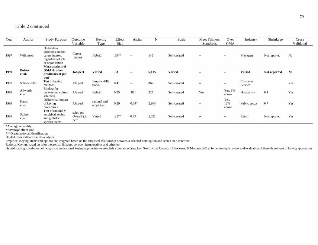
79

Table 2 continued

Year Author Study Purpose Outcome

Variable

Keying

Type

Effect

Size

Alpha N Scale Meet Fairness

Standards

Over

GMA

Industry Shrinkage Cross

Validated

1997 Wilkinson

Do biodata questions predict

career interest

regardless of job or organization

Career interest

Hybrid .63** -- 148 Self-created -- -- Managers Not reported No

1999 Bobko

et al.

Meta-analysis of

GMA & other

predictors of job

perf

Job perf Varied .33 -- 6,115 Varied -- -- Varied Not reported No

1999 Schoen-feldt Test of keying methods

Job perf Empirical/Rational

0.41 -- 867 Self-created -- -- Customer Service

Yes

1999 Allworth

et al.

Biodata for

context and culture selection

Job perf Hybrid 0.35 .82* 325 Self-created Yes Yes, 9%

above Hospitality 0.1 Yes

1999 Karas

et al.

Differential impact

of keying procedures

Job perf rational and

empirical 0.29 0.84* 2,904 Self-created --

Yes,

13% above

Public sector 0.7 Yes

1999 Stokes et al.

Test of rational v

empirical keying and global v

specific items

sales and

Overall job

perf

Varied .21** 0.73 1,621 Self-created -- -- Retail Not reported Yes

*Average reliability.

**Average effect size. ***Organizational Identification

Bolded rows indicate e meta-analyses

Empirical Keying: items and options are weighted based on the empirical relationship between a selected item/option and scores on a criterion. Rational Keying: based on prior theoretical linkages between items/options and criterion

Hybrid Keying: combines both empirical and rational keying approaches to establish a biodata scoring key. See Cucina, Caputo, Thibodeaux, & Maclane (2012) for an in-depth review and evaluation of these three types of keying approaches

80

Table 2 continued

Year Author Study Purpose Outcome

Variable

Keying

Type

Effect

Size

Alpha N Scale Meet Fairness

Standards

Over

GMA

Industry Shrinkage Cross

Validated

1999 West et al.

Assess GMA and

non-cognitive abilities with

Biodata to max.

validity and fairness of

recruiting process

Job perf Hybrid 0.37 0.7 1094 Self-created Yes -- -- -- --

1999 Carlson et al.

Validity

generalization

can be achieved

for biodata

within a single

org as opposed to

multiple orgs

Promotion

rate Hybrid 0.53 -- 7,334

Manager Profile

Record -- -- Varied Not reported Yes

2000 Mount et al.

Incremental

validity of biodata

over gma and personality

Job perf,

retention Hybrid 0.41 0.54 376 Self-created Yes

Yes, by

up to 9%

Administratio

n Not reported Yes

2000 Allworth et al.

Biodata test

construction approach

Job Perf

Construct

from JA only

0.28 0.67 245 Self-created --

Yes,

6.5% above

Customer

Service Not reported No

2000 Harvey-Cook

et al.

Professional entry

level selection Job perf Hybrid 0.23 -- 686

Standard

Application Form -- -- Varied 0.3 Yes

*Average reliability. **Average effect size.

***Organizational Identification

Bolded rows indicate e meta-analyses Empirical Keying: items and options are weighted based on the empirical relationship between a selected item/option and scores on a criterion.

Rational Keying: based on prior theoretical linkages between items/options and criterion

Hybrid Keying: combines both empirical and rational keying approaches to establish a biodata scoring key. See Cucina, Caputo, Thibodeaux, & Maclane (2012) for an in-depth review and evaluation of these three types of keying approaches

81

Table 2 continued

Year Author Study Purpose Outcome

Variable

Keying

Type

Effect

Size

Alpha N Scale Meet Fairness

Standards

Over

GMA

Industry Shrinkage Cross

Validated

2004 Dean

Validating biodata

across multiple performance

criteria:

Training perf

Empirical .39** 0.79 6,036 Self-created --

Yes, 9% above

and

beyond gma

Manu-facturing

0.11*** Yes

2005 Barrick

et al.

Biodata to predict

turnover Turnover --- 0.33 --- 445 Self-created --- -- Varied Not reported No

2006 Harold et al.

Validity of

verifiable and non-

verifiable biodata items, with

incumbents and

applicants

Job perf Hybrid .54** -- 835 Proprietary Kenex scale

-- -- Customer Service

Not reported Yes

2009 Barrick et al.

Assess the

usefulness of pre-

hire variables in predicting

performance and

voluntary turnover

Job

Performanc

e, Turnover

-- .26** -- 354 Self-created -- -- Customer Service

Not reported No

*Average reliability.

**Average effect size. ***Organizational Identification

Bolded rows indicate e meta-analyses

Empirical Keying: items and options are weighted based on the empirical relationship between a selected item/option and scores on a criterion.

Rational Keying: based on prior theoretical linkages between items/options and criterion

Hybrid Keying: combines both empirical and rational keying approaches to establish a biodata scoring key. See Cucina, Caputo, Thibodeaux, & Maclane (2012) for an in-depth review and evaluation of these three types of keying approaches

82

Table 2 continued

Link back to manuscript

Year Author Study Purpose Outcome

Variable

Keying

Type

Effect

Size

Alpha N Scale Meet Fairness

Standards

Over

GMA

Industry Shrinkage Cross

Validated

2009 Becton et al.

Biodata to predict turnover, org

commitment, and

performance in healthcare

Turnover,

Org Commit,

Job Perf

Empirical .33** 0.72 896 Self-created yes -- Healthcare Not reported Yes

2011 Chen et al.

Recruiters

inferences as mediators of

biodata

Hiring recs -- 0.23 0.77 62 Modified Cole et al. (2007)

-- -- Varied Not reported No

2012 Levashina et al.

Reducing faking -- -- -- 0.95 16,304 Self-created -- -- Public sector Not reported --

2013 Dean Biodata fairness v

GMA fairness

Training

Perf Empirical 0.42 -- 3,401 -- Yes -- Public Sector Not reported Yes

*Average reliability.

**Average effect size. ***Organizational Identification

Bolded rows indicate e meta-analyses

Empirical Keying: items and options are weighted based on the empirical relationship between a selected item/option and scores on a criterion. Rational Keying: based on prior theoretical linkages between items/options and criterion

Hybrid Keying: combines both empirical and rational keying approaches to establish a biodata scoring key. See Cucina, Caputo, Thibodeaux, & Maclane (2012) for an in-depth review and evaluation of these three types of keying approaches

83

Table 3

Overview of Text analytics and the Marker Word Hypothesis Used in Psychological and Computer Science Research

Year Author Study Purpose Hypothesis/Theory Method Findings

1975 Tucker &

Rosenberg

Differentiate the speech of

schizophrenics from non-

schizophrenics via text

analytics

No theory cited, referenced past works

that attempted to use language used to

diagnose a mental health disorder, past

work focused on the structure of

language (e.g. grammar and syntax) or

content analysis of themes.

Used the General Inquirer Computer

Content Analysis Program with the

Harvard III Psychosocial Dictionary.

Only analyzed 600 words from each

person. Used mean comparisons and

factor analysis.

Categories like “time reference,” “sense,” and

“attempt” differentiated between schizophrenics

and non-schizophrenics. Overall, the categories

demonstrated themes around confusion, distress,

and self-concern, and were consistent with clinical

experience.

1982 Oxman et

al.

Test 3 theories about

paranoia via text analytics.

Discussed three theories of paranoia.

Paranoia as a subtype of

schizophrenia, a separate mental

disorder, or on a continuum from

normal to abnormal.

Used the General Inquirer Computer

Content Analysis Program with the

Harvard III Psychosocial Dictionary.

Only analyzed 600 words from each

person. Used mean comparisons and

factor analysis.

Results suggested paranoia as a separate mental

disorder rather than a sub-type of schizophrenia or

on a scale from normal to abnormal. Paranoid

participants used more abstract self-reference

words, used neutral affect words when discussing

others, and tended to use more words expressing

warmth and intimacy. Paranoid participants were

classified correctly 80% of the time when using

speech samples.

1986 Scherwitz

et al.

Assess risk factor of Type A

for coronary heart disease

(CHD)

Type A behavior predicts CHD

Count of first, person pronouns (I, me,

my) and logistic regression to predict

(CHD) and heart attack.

Use of first-person pronouns (I, me, my) predicted

CHD, mortality from CHD, and fatal heart attacks.

1997 Pennebaker

et al.

Examined the extent to

which discussing the death

of a loved one was

predictive of later physical

and mental health

Disclosure theory: confronting

upsetting topics reduces the

constraints or inhibitions associated

with not talking about the events.

Differential emotion: using more

negative words leads to health

improvements.

LIWC correlated with self-reports of

mental and physical health

Use of more positive words and insight words like

“think,” “know,” “consider” were associated with

health.

2001 Cheng et

al.

Accurately predict a

person’s sex based on text

data.

Can the sex of an author be identified

from a short text document?

LIWC to identify psycholinguistic and

sex cues and computer science

algorithms for sex identification based

on the authors chosen LIWC

categories and sub-categories

Able to predict author sex with 85% accuracy.

Words indicative of sex were function words

(articles, conjunctions, etc.), word features (total

number of words, avg character length per word,

etc.), and structural features (number of sentences,

paragraphs, etc.)

2001 Danner et

al.

Examine the relationship

between emotional text

content and mortality in late

adulthood (75-95)

Emotions reflect patterns of adaptive

or maladaptive coping

Self-created coding process developed

for study and regression analysis

Positive emotion words (accomplishment,

happiness, hope, love) were related to longevity 60

years later. 1% increase in positive words decreased

mortality rate by 1.4%.

84

Table 3 continued

Link back to manuscript

Year Author Study Purpose Hypothesis/Theory Method Findings

2001 Pennebaker

& Stone

Investigate links between

aging and language use

Theories and hypothesis centered on

aging and: affect, social relationships,

time orientation, and cognitive ability

LIWC (14 categories only) correlated

with and regressed on age

As age increased, use of positive affect words,

present, and future tense verb use increased

2001 Stirman &

Pennebaker

Investigated whether word

usage and word styles

differentiated poets who

committed suicide versus

those who did not.

Social Integration/disengagement

Theory

Used LIWC to identify words and

stylometric features that distinguished

poets who committed suicide from

those who did not

Poets who committed suicide tended to use more

first-person, singular pronouns (I, me, my) than

poets who did not.

2010 Holtgraves

Investigated how language

used in text messaging

varies as a function of

personality, sex,

interpersonal context.

Hypothesis based on prior findings

looking at the links between language

use and extraversion, agreeableness,

and neuroticism

Used LIWC correlated with

Goldberg’s (1992) measure of the Big

Five looking at extraversion,

agreeableness, and neuroticism only.

Extraversion was correlated with personal

pronouns, agreeableness with positive emotion

words and swearing, neuroticism with negative

emotion words. Females used more social words,

personal pronouns, and used more emoticons.

Males used more swear words, more overall words.

Slang and emoticons were used more with friends

and romantic partners

2013 Schultheiss

Looked to see if motivations

(specifically, McClelland’s

need typology) could be

inferred from language use.

Sought to extend McClelland’s need

theory using new methodology

(computerized text analytics)

Used LIWC categories correlated with

measures of McClelland’s needs.

Power was related to anger categorized words.

Achievement with achievement, positive emotion,

optimism, and occupation words. Affiliation with

social, friend, third-person pronouns, and positive

feeling words.

2013 Tomlinson

et al.

Examined whether it was

possible to predict

conscientious using

Facebook posts.

No theory cited; hypothesis was that

verb usage that is less specific is

predictive of conscientiousness.

Used WordNet and parsed Facebook

posts into subjects and verbs.

More specific and less objective verbs were

correlated .27 with conscientious. Specific verb

examples: donated, stabbed versus gave and hurt.

85

Table 4.

Descriptive Statistics: LIWC Categories for Hypothesis 2-5 with Base Rate Comparisons (Sub-Sample)

LIWC categories for hypothesis 2-5 M SD Skew Kurtosis

1st person singular pronouns 1.22 (4.99) 1.66 (2.46) 1.81 2.97

1st person plural pronouns 0.08 (0.72) 0.19 (0.83) 4.46 27.39

2nd person pronouns 0.04 (1.70) 0.14 (1.35) 5.02 30.36

3rd person singular pronouns 0.02 (1.88) 0.11 (1.53) 8.57 100.38

3rd person plural pronouns 0.20 (0.66) 0.32 (0.60) 2.60 8.90

Impersonal pronouns 0.92 (5.26) 0.71 (1.62) 1.24 2.07

Auxiliary verbs 1.42 (8.53) 1.33 (2.04) 1.56 2.79

Verbs 4.79 (16.44) 2.32 (2.93) 0.83 0.97

Positive emotion words 2.83 (3.67) 1.22 (1.63) 0.41 -0.00

Negative emotion words 0.53 (1.84) 0.52 (1.09) 2.05 6.49

Differentiation words 0.55 (2.99) 0.50 (1.18) 1.91 5.93

Conjunctions 6.25 (5.90) 2.04 (1.57) -0.41 0.44

Words longer than 6 characters 40.18 (15.60) 6.29 (3.76) -0.78 3.06

Prepositions 12.05 (12.93) 3.08 (2.11) -1.00 3.07

Cognitive process words 5.73 (10.61) 2.03 (3.02) 0.47 1.56

Causal words 1.96 (1.40) 1.01 (0.73) 0.83 1.77

Insight words 1.98 (2.16) 1.00 (1.08) 1.14 3.86

Note. Bolded values indicate skewness and kurtosis exceed ±2. N = 667. Values in

parentheses are LIWC reported average base rates and standard deviations

Link back to manuscript

86

Table 5.

Impression Management Questionnaire (Wayne & Liden, 1995)

Link back to manuscript

Dimensions Item Text

Other-Impression Management

In the past 3 months, to what

extent did you

O-IM1 Do personal favors for your supervisor (for example, getting him

or her a cup of coffee or coke, etc.)

O-IM2 Offer to do something for your supervisor which you were not

required to do; that is, you did it as a personal favor to him or

her

O-IM3 Complimented your immediate supervisor on his or her dress or

appearance

O-IM4 Praise your immediate supervisor on his or her accomplishments

O-IM5 Take an interest in your supervisor’s personal life

Self-Impression Management

In the past 3 months, to what

extent did you

S-IM1 Try to be polite when interacting with your supervisor

S-IM2 Try to be a friendly person when interacting with your

supervisor

S-IM3 Try to act as a “model” employee by, for example, never taking

longer than the established time for lunch

S-IM4 Work hard when you know the results will be seen by your

supervisor

S-IM5 Let your supervisor know that you try and do a good job in your

work

87

Table 6

The Spot-The-Word Test (Baddeley et al., 1993)

Link back to manuscript

Items

slank – chariot coracle – prestasis

lentil – glotex paramour – imbulasm

stamen - dombus dallow – ocatroon

loba – comet fleggary – carnation

pylon – strion liminoid – agnostic

scrapten – flannel naquescent – plinth

fender – ullus thole – leptine

ragsupr – joust crattish – reform

milliary – mantis wraith – stribble

sterile – palth metulate – pristine

proctive – monotheism pauper – progotic

gilivular – stallion aurant – baleen

intervantation – rictus palindrome – lentathic

byzantine – chloriant hedgehog – mordler

monologue – rufine prassy – ferret

elegy – festant torbate – drumlin

malign – vago texture – disenrupted

exonize – gelding isomorphic – thassiary

bulliner – trireme fremoid – vitriol

visage – hyperlistic farrago – gesticity

frion – oratory minidyne – hermeneutic

meridian – phillidism pusality – chaos

grottle – strumpet devastate – prallage

equine – psynomy peremptory – paralepsy

baggalette – riposte chalper – camera

valance – plesmiod roster – falluate

introvert – vinadism scaline – accolade

penumbra – rubiant methagenate – pleonasm

breen – maligner drobble – infiltrate

gammon - unterried mystical – harreen

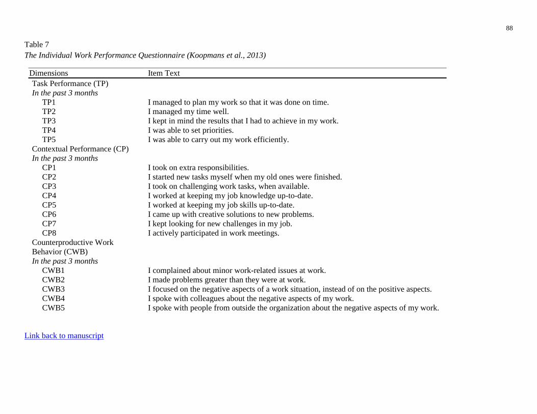
88

Table 7

The Individual Work Performance Questionnaire (Koopmans et al., 2013)

Link back to manuscript

Dimensions Item Text

Task Performance (TP)

In the past 3 months

TP1 I managed to plan my work so that it was done on time.

TP2 I managed my time well.

TP3 I kept in mind the results that I had to achieve in my work.

TP4 I was able to set priorities.

TP5 I was able to carry out my work efficiently.

Contextual Performance (CP)

In the past 3 months

CP1 I took on extra responsibilities.

CP2 I started new tasks myself when my old ones were finished.

CP3 I took on challenging work tasks, when available.

CP4 I worked at keeping my job knowledge up-to-date.

CP5 I worked at keeping my job skills up-to-date.

CP6 I came up with creative solutions to new problems.

CP7 I kept looking for new challenges in my job.

CP8 I actively participated in work meetings.

Counterproductive Work

Behavior (CWB)

In the past 3 months

CWB1 I complained about minor work-related issues at work.

CWB2 I made problems greater than they were at work.

CWB3 I focused on the negative aspects of a work situation, instead of on the positive aspects.

CWB4 I spoke with colleagues about the negative aspects of my work.

CWB5 I spoke with people from outside the organization about the negative aspects of my work.

89

Table 8

Overview of Evidence for the Validity and Reliability of the Individual Work Performance Questionnaire (Koopmans et al., 2013).

Link back to manuscript

Year Author Article Title Sample Size Demographics Reliability Validity Dimensions Items

2013 Koopmans

et al.

Development of an

individual work

performance questionnaire

1,181 Dutch workers,

jobs spanned blue

to white collar

0.78-0.851 across

all dimensions

N/A TP

CP

AP

CWB

14 total

4 (TP)

2 (CP)

3 (AP)

5 (CWB)

2014 Koopmans

et al.

Improving the individual

work performance

questionnaire using Rasch

analysis.

1,424 Dutch workers,

jobs spanned blue

to white collar

0.81 (TP)1

0.85 (CP)1

0.74 (CWB)1

N/A TP

CP

CWB

18 Total

5 (TP)

8 (CP)

5 (CWB)

2014 Koopmans

et al.

Responsiveness of the

individual work

performance questionnaire.

412 Financial workers

in the Netherlands

0.78 (TP)2

0.85 (CP)2

0.79 (CWB)2

Convergent Validity

Presenteeism: 0.18 (TP), 0.22 (CP), -0.11 (CWB)

Job Sat: 0.12 (TP), 0.17 (CP), -0.24 (CWB)

Work Engagement: 0.19 (TP), 0.29 (CP), -0.23 (CWB)

Work Ability: 0.16 (TP), 0.26 (CP), -0.23 (CWB)

Manager Rating: 0.16 (TP), 0.26 (CP), -0.02 (CWB)

Work Quality: 0.20 (TP), 0.18 (CP), -0.06 (CWB)

Work Quantity: 0.11 (TP), 0.19 (CP), -0.02 (CWB)

Discriminant Validity

Need for Recovery: -0.15 (TP), -0.11 (CP), 0.16 (CWB)

General Health: -0.07 (TP), 0.08 (CP), 0.02 (CWB)

Vitality: 0.23 (TP), 0.29 (CP), -0.03 (CWB)

Exhaustion: -0.23 (TP), -0.13 (CP), 0.23 (CWB)

Sickness absenteeism: -0.14 (TP), -0.08 (CP), -0.09 (CWB)

TP

CP

CWB

18 Total

5 (TP)

8 (CP)

5 (CWB)

2014 Koopmans

et al.

Construct validity of the

individual work

performance questionnaire.

1,424 Dutch workers,

jobs spanned blue

to white collar

N/A Convergent Validity

HPQ Absolute Presenteeism: 0.39 (TP), 0.33 (CP) -0.16 (CWB)

HPQ Relative Presenteeism: 0.09 (TP), 0.11) (CP), 0.07 (CWB)

UWES: 0.35 (TP), 0.43 (CP), -0.31 (CWB)

Discriminant Validity

Defined as the extent to which a measure can differentiate known

groups. For example, higher job satisfaction would have a higher

task and contextual scores and lower scores than individuals with

low job satisfaction. (see p. 332 for definition and pp. 334-335

for results and figures)

TP

CP

CWB

18 Total

5 (TP)

8 (CP)

5 (CWB)

2015 Koopmans

et al.

Cross-cultural adaptation of

the individual

work performance

questionnaire

40 American workers,

jobs spanned blue

to white collar

0.79 (TP)2

0.83 (CP)2

0.89 (CWB)2

N/A TP

CP

CWB

18 Total

5 (TP)

8 (CP)

5 (CWB)

2014 Landers et

al.

Validation of the beneficial

and harmful work-related

social media behavioral

taxonomies: Development

of the work-related social

media questionnaire.

100 Mturk sample,

mostly White,

older (M = 31.5)

0.86 (TP)2

0.77 (CP)2

0.86 (CWB)2

0.87 (AP)2

Correlated with the Work-related Social Media Questionnaire

(WSMQ, + or -).

WSMQ(+) short form

0.02 (task), 0.10 (contextual), 0.12 (adaptive), -0.01 (CWB)

WSMQ(-) short form

-0.40 (task), -0.45 (contextual), -0.48 (adaptive), 0.32 (CWB)

TP = Task Performance. CP = Contextual Performance. CWB = counterproductive work behavior. AP = adaptive performance 1: person separation index (PSI) estimates the internal consistency of a scale, it’s similar to Cronbach’s alpha, only it uses the logit scale estimates as opposed to the raw scores. It is interpreted in a similar manner, a minimum

value of 0.70 is required for group use and 0.85 for individual use.

2: Cronbach’s Alpha

90

Table 9

Benchmark Scores for the Individual Work Performance Questionnaire

Blue Collar Pink Collar (service industry) White Collar

TP CP CWB TP CP CWB TP CP CWB

Very Low ≤2.00 ≤ 1.25 ≤ 0.20 ≤ 1.83 ≤ 1.25 ≤ 0.00 ≤ 1.83 ≤ 1.37 ≤ 0.40

(≤ 10th percentile) Low 2.01-2.49 1.26-1.74 0.21-0.59 1.84-2.32 1.26-1.74 0.01-0.59 1.84-2.16 1.38-1.87 0.41-0.79

(10-25th percentile) Average 2.50-3.16 1.75-2.99 0.60-1.39 2.33-2.99 1.75-2.87 0.60-1.59 2.17-2.99 1.88-.287 0.80-1.59

(25-75th percentile) High 3.17-3.49 3.00-3.24 1.40-1.79 3.00-3.49 2.88-3.12 1.60-1.99 3.00-3.32 2.88-3.24 1.60-1.99

(75-90th percentile) Very High ≥ 3.50 ≥ 3.25 ≥ 1.80 ≥ 3.50 ≥ 3.13 ≥ 2.00 ≥ 3.33 ≥ 3.25 ≥ 2.00

(≥ 90th percentile) TP= Task Performance. CP= Contextual Performance. CWB= Counter Productive Work Behaviors

Link back to manuscript

91

Table 10

Descriptive Statistics: Primary Study Variables by Sex (Full Sample)

Gender

Female Male

Primary study variables M SD Skew Kurtosis M SD Skew Kurtosis

Corroboration Variables

Impression Management

Other 16.22 7.64 0.30 -0.90 16.36 7.60 0.27 -0.74

Impression Management Self 27.84 5.95 -1.39 2.29 26.13 6.11 -0.83 0.91

Verbal Intelligence 48.50 9.10 -2.90 10.49 44.27 12.98 -1.84 2.99

Independent Variables

1st person singular pronouns 1.11 1.77 2.03 3.96 0.85 1.50 2.38 5.96

1st person plural pronouns 0.06 0.19 5.70 40.83 0.05 0.18 5.51 38.56

2nd person pronouns 0.03 0.14 6.36 45.46 0.04 0.21 7.04 57.91

3rd person singular pronouns 0.02 0.07 5.11 28.64 0.01 0.08 15.20 274.16

3rd person plural pronouns 0.20 0.34 2.38 6.94 0.10 0.26 4.25 23.68

impersonal pronouns 0.74 0.73 1.35 2.21 0.64 0.75 1.41 2.05

auxiliary verbs 1.34 1.57 2.26 7.42 1.09 1.45 2.57 11.87

verbs 4.64 2.65 0.75 0.70 4.04 3.14 1.73 8.41

positive emotion words 2.70 1.61 1.02 3.44 2.24 1.77 0.95 2.44

negative emotion words 0.43 0.50 1.74 4.83 0.44 0.68 3.14 14.44

differentiation words 0.54 0.55 1.69 4.47 0.38 0.61 4.30 36.53

conjunctions 5.81 2.49 -0.47 0.02 4.48 3.02 -0.13 -0.98

words longer than 6 characters 41.13 7.78 -0.91 3.47 36.81 11.85 -1.05 1.25

prepositions 11.25 3.97 -0.93 1.09 9.30 5.31 -0.52 -0.59

cognitive process words 5.30 2.44 0.29 0.84 4.43 3.04 0.36 0.59

causal words 1.69 1.10 1.12 4.31 1.50 1.34 0.78 0.39

insight words 1.82 1.19 1.21 3.93 1.68 1.46 1.27 3.11

Dependent Variables

Task Performance 3.11 0.69 -0.84 0.63 2.85 0.79 -0.62 0.06

Note. Bolded values indicate skewness and kurtosis exceeds ±2. Female (n = 280 / 35%), Male (n = 530 / 65%)

Link back to manuscript

92

Table 11

Descriptive Statistics: Primary Study Variables by Race: White, Asian, Hispanic/Latino (Full Sample)

Link back to manuscript

Primary Study Variables M SD Skew Kurtosis M SD Skew Kurtosis M SD Skew Kurtosis

Corroboration Variables

Impression Management Other 15.73 7.65 0.36 -0.80 18.05 7.27 -0.04 -0.74 13.79 5.19 0.92 1.56

Impression Management Self 27.05 6.15 -1.17 1.76 25.95 5.93 -0.64 0.12 24.14 7.03 -0.88 0.76

Verbal Intelligence 47.90 8.86 -2.77 9.92 40.56 16.86 -1.12 0.05 43.39 12.31 -1.80 4.02

Independent Variables

1st person singular pronouns 1.11 1.72 1.97 3.71 0.70 1.45 2.91 9.41 0.31 0.51 1.78 2.36

1st person plural pronouns 0.06 0.20 5.52 38.28 0.04 0.16 5.85 38.72 0.04 0.11 2.84 6.89

2nd person pronouns 0.03 0.15 8.78 97.58 0.06 0.27 5.52 34.49 0.00 0.00 0.00 0.00

3rd person singular pronouns 0.01 0.07 5.79 37.40 0.01 0.11 13.95 198.78 0.00 0.00 0.00 0.00

3rd person plural pronouns 0.16 0.32 3.13 12.86 0.06 0.20 3.82 14.37 0.13 0.33 3.30 11.98

impersonal pronouns 0.77 0.80 1.31 1.70 0.48 0.62 1.18 0.39 0.40 0.45 0.76 -0.68

auxiliary verbs 1.34 1.52 1.87 5.02 0.92 1.56 3.86 22.54 0.67 0.75 1.12 0.70

verbs 4.59 2.99 1.51 7.92 3.61 3.09 1.51 4.94 2.71 1.92 0.22 -0.80

positive emotion words 2.64 1.64 0.83 2.41 1.87 1.91 1.46 4.31 2.12 1.58 0.16 -0.90

negative emotion words 0.45 0.58 2.56 11.17 0.38 0.76 3.59 16.28 0.39 0.47 2.17 7.24

differentiation words 0.50 0.63 3.75 30.21 0.32 0.53 2.48 7.88 0.37 0.54 2.25 6.84

conjunctions 5.57 2.70 -0.49 -0.20 3.35 2.98 0.30 -1.11 4.38 2.57 -0.50 -0.76

words longer than 6 characters 40.61 7.98 -0.66 3.91 31.96 13.91 -0.59 -0.77 39.39 11.88 -2.10 4.43

prepositions 10.79 4.31 -0.86 0.61 8.08 6.12 -0.15 -1.23 8.13 4.21 -0.68 -0.73

cognitive process words 5.18 2.61 0.28 0.89 3.65 3.31 0.69 0.92 4.53 3.02 0.43 -0.07

causal words 1.76 1.24 0.89 1.95 1.06 1.22 1.04 0.58 1.40 1.50 1.12 0.85

insight words 1.80 1.30 1.48 4.71 1.53 1.55 1.06 1.79 2.18 1.65 0.99 1.97

Dependent Variables

Task Performance 3.01 0.72 -0.79 0.73 2.76 0.81 -0.37 -0.60 2.93 0.91 -1.11 1.14

White Asain Hispanic/Latino

Note: Bolded values indicates skewness and kurtosis exceeds ±2. White (n = 530 / 63%). Asian (n = 222 / 26%). Hispanic/Latino (n = 28 / 3%).

93

Table 11

Descriptive Statistics: Primary Study Variables by Race: Other, Black, Hawaiian/Pacific Islander, American Indian/Alaskan Indian (Full Sample)

Cont’d

Link back to manuscript

Primary Study Variables M SD Skew Kurtosis M SD Skew Kurtosis M SD Skew Kurtosis M SD Skew Kurtosis

Corroboration Variables

Impression Management Other 16.81 9.07 0.33 -0.93 15.80 8.08 0.69 -0.14 16.00 - - - 13.00 - - -

Impression Management Self 27.10 6.07 -0.62 -0.01 28.64 4.61 -0.09 -1.20 34.00 - - - 28.00 - - -

Verbal Intelligence 45.58 8.35 -1.12 0.84 47.56 5.68 -0.38 0.79 55.00 - - - 50.00 - - -

Independent Variables

1st person singular pronouns 0.88 1.31 1.57 1.20 0.43 0.91 3.24 12.02 - - - - - - - -

1st person plural pronouns 0.08 0.18 2.08 3.00 0.01 0.05 5.00 25.00 - - - - - - - -

2nd person pronouns 0.07 0.24 4.06 17.96 0.04 0.17 4.38 19.87 - - - - - - - -

3rd person singular pronouns 0.00 0.00 0.00 0.00 0.01 0.05 5.00 25.00 - - - - - - - -

3rd person plural pronouns 0.13 0.27 2.90 9.16 0.17 0.30 2.76 8.89 - - - - - - - -

impersonal pronouns 0.62 0.48 0.12 -1.22 0.62 0.58 0.73 -0.66 - - - - 0.53 - - -

auxiliary verbs 1.05 1.27 1.68 3.45 0.93 1.00 1.80 3.92 - - - - 0.53 - - -

verbs 4.48 2.62 0.82 1.12 4.16 2.33 2.16 7.68 0.85 - - - 3.74 - - -

positive emotion words 2.25 1.59 1.09 1.10 2.46 1.29 0.46 0.04 1.71 - - - 2.67 - - -

negative emotion words 0.48 0.52 0.69 -0.91 0.53 0.45 0.54 -0.05 - - - - 1.60 - - -

differentiation words 0.35 0.42 1.23 0.94 0.33 0.32 0.98 1.16 - - - - 0.53 - - -

conjunctions 4.88 2.67 -0.13 -0.47 6.00 2.26 -0.22 1.36 4.27 - - - 8.56 - - -

words longer than 6 characters 37.15 11.38 -1.49 4.16 44.25 6.58 -0.06 -0.26 52.14 - - - 48.66 - - -

prepositions 10.25 4.54 -0.30 1.12 10.88 3.64 -1.21 2.34 11.11 - - - 11.23 - - -

cognitive process words 4.35 2.38 0.12 -0.36 5.60 2.15 -0.05 0.18 1.71 - - - 3.21 - - -

causal words 1.43 0.92 -0.13 -0.87 2.12 1.22 0.39 -0.18 0.85 - - - 1.60 - - -

insight words 1.43 1.00 0.48 -0.15 1.99 1.09 0.98 0.98 0.85 - - - 1.07 - - -

Dependent Variables

Task Performance 2.77 0.99 -0.55 -0.68 3.21 0.62 -0.56 -0.28 3.00 - - - 2.80 - - -

Other African American Hawaiin/Pacific Islander American Indian/Alaskan Indian

Note: bolded values indicates skewness and kurtosis exceeds ±2. Other (n = 31 / 4%). African American (n = 25 / 3%). Native Hawaiian or Other Pacific Islander (n = 1 / 0.001%). American Indian or

Alaska Native (n = 1 / 0.001%).

94

Table 12

Descriptive Statistics: Primary Study Variables by Education: Bachelor’s, Master’s, Some College, Doctorate (Full Sample)

Link back to manuscript

Primary Study Variables M SD Skew Kurtosis M SD Skew Kurtosis M SD Skew Kurtosis M SD Skew Kurtosis

Corroboration Variables

Impression Management Other 15.92 7.34 0.23 -0.86 16.00 7.34 0.40 -0.69 16.69 8.39 0.33 -0.77 18.67 7.27 -0.13 -0.75

Impression Management Self 27.20 5.76 -0.94 1.01 26.62 5.35 -0.63 0.26 28.37 5.85 -1.17 1.86 26.12 6.54 -1.14 1.97

Verbal Intelligence 46.63 10.38 -2.37 6.19 46.85 11.13 -2.07 5.36 45.85 11.53 -2.12 4.44 39.17 20.04 -0.94 -0.71

Independent Variables

1st person singular pronouns 0.89 1.46 2.10 4.08 0.67 1.11 2.22 5.20 1.29 2.03 1.69 2.06 0.88 1.63 1.96 2.94

1st person plural pronouns 0.05 0.17 4.37 23.47 0.04 0.20 7.26 59.41 0.06 0.18 3.81 16.19 0.02 0.05 3.83 14.61

2nd person pronouns 0.04 0.20 7.59 66.98 0.05 0.19 4.92 27.12 0.03 0.22 9.19 88.74 0.05 0.22 4.40 18.88

3rd person singular pronouns 0.01 0.10 11.05 147.90 0.01 0.04 5.32 27.55 0.01 0.07 5.47 32.22 0.00 0.03 7.62 58.00

3rd person plural pronouns 0.14 0.29 3.00 11.22 0.11 0.27 3.51 15.34 0.17 0.35 3.18 13.75 0.04 0.10 3.38 12.84

impersonal pronouns 0.74 0.74 1.15 1.15 0.64 0.68 1.63 4.32 0.79 0.87 1.11 0.60 0.30 0.62 3.27 13.10

auxiliary verbs 1.16 1.25 1.67 3.76 1.03 1.43 3.33 17.33 1.52 1.77 1.38 1.51 1.32 2.42 3.08 11.47

verbs 4.35 2.56 0.60 0.65 3.68 2.53 1.03 2.39 4.77 3.00 0.44 -0.11 4.31 4.17 1.57 3.37

positive emotion words 2.55 1.45 0.28 -0.25 2.12 1.49 1.33 5.30 2.78 2.13 0.90 2.23 1.55 2.28 2.71 9.85

negative emotion words 0.44 0.53 2.67 14.21 0.45 0.71 2.80 9.29 0.43 0.48 0.87 -0.21 0.30 0.81 4.67 25.93

differentiation words 0.46 0.50 1.56 3.20 0.38 0.50 2.50 10.22 0.59 0.92 4.41 29.17 0.22 0.51 3.99 19.75

conjunctions 5.46 2.60 -0.40 -0.07 4.54 2.82 -0.05 -0.52 5.35 3.00 -0.66 -0.67 3.08 3.08 0.39 -1.35

words longer than 6 characters 39.93 7.82 -1.05 3.65 40.61 11.04 -1.33 4.19 36.58 10.63 -0.90 1.41 28.65 15.17 -0.05 -1.38

prepositions 10.91 4.09 -0.87 1.00 9.92 5.11 -0.62 -0.21 9.83 4.95 -0.82 -0.18 7.56 6.58 0.15 -1.17

cognitive process words 5.18 2.51 0.04 0.48 4.66 2.70 0.14 0.24 4.82 3.06 -0.01 -0.58 2.61 3.65 2.26 7.05

causal words 1.75 1.19 0.53 0.57 1.56 1.28 0.76 0.41 1.47 1.28 1.05 1.29 0.80 1.26 2.28 6.05

insight words 1.86 1.23 1.14 3.31 1.88 1.52 1.20 2.39 1.54 1.12 0.31 -0.41 1.14 1.78 2.52 7.74

Dependent Variables 0.00

Task Performance 3.01 -0.77 0.70 2.97 0.69 -0.94 1.01 2.85 0.88 -0.43 -0.73 2.82 0.84 -0.77 0.16

Note. Bolded values indicates skewness and kurtosis exceeds ±2. Bachelors (n = 356 / 44%). Masters (n = 149 / 18%). Some College (n = 104 / 13%). Doctorate (n = 58 / 7%).

Bachelors Masters Some College Doctorate

95

Table 12

Descriptive Statistics: Primary Study Variables by Education: Professional, Associates, High School, Trade/Vocational/Technical (Full Sample)

Link back to manuscript

Primary Study Variables M SD Skew Kurtosis M SD Skew Kurtosis M SD Skew Kurtosis M SD Skew Kurtosis

Corroboration Variables

Impression Management Other 16.53 7.32 0.07 -0.89 16.18 8.70 0.43 -0.98 15.43 7.12 0.20 -0.96 17.71 9.10 0.44 -0.91

Impression Management Self 23.75 6.89 -0.41 -0.84 24.61 7.45 -1.35 1.58 23.73 6.99 -0.88 1.01 27.39 6.87 -1.52 3.00

Verbal Intelligence 39.83 16.67 -1.30 0.59 47.74 7.90 -2.44 8.46 45.73 8.27 -1.99 5.86 47.32 8.94 -2.93 11.24

Independent Variables

1st person singular pronouns 1.17 2.18 2.63 6.84 0.69 1.08 1.68 2.14 1.03 1.85 2.48 6.71 1.78 2.42 1.45 1.06

1st person plural pronouns 0.04 0.15 4.38 19.14 0.12 0.38 3.79 14.72 0.02 0.08 3.63 12.36 0.05 0.15 3.10 9.37

2nd person pronouns 0.01 0.05 4.88 24.40 0.02 0.11 4.62 21.57 0.05 0.19 3.75 13.31 0.01 0.04 4.26 18.76

3rd person singular pronouns 0.01 0.03 4.38 18.41 0.01 0.04 6.16 38.00 0.01 0.04 6.08 37.00 0.02 0.06 3.11 8.76

3rd person plural pronouns 0.10 0.26 2.80 7.61 0.11 0.26 2.38 4.60 0.19 0.46 3.00 9.19 0.15 0.20 1.30 1.02

impersonal pronouns 0.47 0.55 1.04 0.09 0.61 0.70 1.39 1.81 0.53 0.68 0.88 -0.70 0.82 0.95 1.85 4.15

auxiliary verbs 0.76 1.12 2.03 4.94 1.04 1.34 1.80 2.96 1.12 1.59 1.80 3.11 1.55 1.68 1.05 0.33

verbs 3.80 4.81 3.65 18.05 3.71 2.44 0.59 0.08 4.56 3.81 1.15 1.93 4.74 3.35 0.08 -0.90

positive emotion words 1.95 1.85 0.78 0.11 2.26 1.76 0.65 0.79 2.18 1.85 0.47 -0.59 3.28 1.94 -0.07 -0.35

negative emotion words 0.31 0.50 2.36 6.81 0.61 1.04 2.58 7.32 0.46 0.65 1.55 1.91 0.51 0.52 0.61 -0.75

differentiation words 0.24 0.30 1.09 0.13 0.59 0.71 1.54 2.26 0.36 0.54 2.21 5.38 0.55 0.68 1.95 3.81

conjunctions 3.46 3.14 0.27 -1.38 5.13 3.20 -0.23 -0.89 3.94 3.20 0.21 -1.13 5.99 2.92 -0.88 -0.15

words longer than 6 characters 32.03 13.69 -0.67 -0.98 39.36 12.19 -1.72 3.07 37.92 13.29 -1.23 1.97 39.75 8.10 -0.72 1.35

prepositions 8.17 6.34 -0.15 -1.26 9.15 5.11 -0.64 -0.36 8.05 5.66 -0.26 -1.48 10.06 4.72 -0.65 -0.59

cognitive process words 3.14 2.60 0.11 -1.42 5.16 3.01 -0.01 -0.10 4.59 3.37 0.69 1.46 5.31 2.70 0.71 1.51

causal words 1.11 1.02 0.37 -1.00 1.83 1.28 0.17 -0.71 1.60 1.73 1.80 5.12 1.47 0.98 -0.24 -1.25

insight words 1.31 1.24 0.49 -1.03 1.59 1.20 0.62 -0.12 1.66 1.71 1.76 5.08 2.05 1.67 1.11 2.23

Dependent Variables

Task Performance 2.70 0.76 -0.30 -0.51 2.91 0.79 -1.00 0.99 2.73 0.84 -0.08 -0.94 3.18 0.62 -0.70 0.34

Note: bolded values indicate and kurtosis exceeds ±2. Professional (n = 40 / 5%). Associates (n = 39 / 5%). High School (n = 37 / 5%). Trade, Vocational, or Technical (n = 28 / 3%).

AssociatesProfessional Trade, Vocational, or TechnicalHigh School

96

Table 13a

Descriptive Statistics: Tenure (Full Sample)

M SD Skew Kurtosis

Tenure 3.45 3.52 2.56 9.66

Note. Bolded values indicate skewness and

kurtosis exceeds ±2. N = 809

97

Table 13b

Descriptive Statistics: Tenure Correlated with Hypothesis Variables (Full Sample)

Link back to manuscript

Primary Study Variables Tenure

Corroboration Variables

Impression Management

Other '0.03

Impression Management Self -0.14

Verbal Intelligence -0.02

Independent Variables

1st person singular pronouns 0.01

1st person plural pronouns 0.03

2nd person pronouns -0.01

3rd person singular pronouns 0.05

3rd person plural pronouns -0.05

impersonal pronouns -0.08

auxiliary verbs 0.06

verbs 0.01

positive emotion words -0.06

negative emotion words -0.05

differentiation words -0.05

conjunctions -0.10

words longer than 6

characters -0.04

prepositions -0.06

cognitive process words -0.14

causal words -0.08

insight words -0.13

Dependent Variables

Task Performance -0.09

Italics values indicate p < .05, bolded values

indicate p < .001, N = 809

99

Table 14

Descriptive Statistics: Hypothesis Variables by Sex (Sub-Sample)

Gender

Female Male

Primary Study variables M SD Skew Kurtosis M SD Skew Kurtosis

Corroboration Variables

Impression Management Other 16.36 7.42 0.24 -1.00 15.59 7.24 0.53 -0.32

Impression Management Self 28.60 5.25 -1.37 2.67 26.65 5.82 -0.83 1.17

Verbal Intelligence 49.38 7.90 -3.12 13.34 47.17 9.22 -2.40 7.66

Independent Variables

1st person singular pronouns 1.39 1.89 1.66 2.25 1.10 1.47 1.84 3.13

1st person plural pronouns 0.08 0.21 5.88 44.03 0.08 0.19 3.10 10.40

2nd person pronouns 0.03 0.12 6.51 55.08 0.05 0.15 4.37 21.96

3rd person singular pronouns 0.03 0.09 3.92 16.55 0.02 0.12 9.67 110.94

3rd person plural pronouns 0.25 0.33 1.94 4.42 0.16 0.30 3.30 14.68

impersonal pronouns 0.89 0.69 1.45 3.04 0.94 0.74 1.11 1.58

auxiliary verbs 1.51 1.45 1.76 3.39 1.36 1.23 1.25 1.35

verbs 5.15 2.38 1.02 1.31 4.53 2.24 0.66 0.46

positive emotion words 2.88 1.24 0.53 0.19 2.80 1.21 0.32 -0.16

negative emotion words 0.50 0.50 1.92 6.56 0.55 0.54 2.13 6.48

differentiation words 0.60 0.48 1.94 8.25 0.51 0.51 1.96 4.85

conjunctions 6.71 1.89 -0.69 1.06 5.91 2.08 -0.21’ 0.38

words longer than 6 characters 40.80 6.06 -0.35 0.16 39.73 6.43 -1.03 4.64

prepositions 12.50 2.99 -0.82 2.99 11.72 3.11 -1.14 3.17

cognitive process words 5.70 2.14 0.83 2.22 5.76 1.96 0.12 0.93

causal words 1.80 0.90 0.51 0.29 2.07 1.08 0.90 1.98

insight words 1.95 1.06 1.61 7.00 2.00 0.95 0.68 0.32

Dependent Variables

Task Performance 3.19 0.67 -0.90 0.72 2.96 0.74 -0.81 1.21

Note. Female (n = 260 / 39%), Male (n = 407 / 61%) bolded values indicate skewness and kurtosis exceed ±2

Link back to manuscript

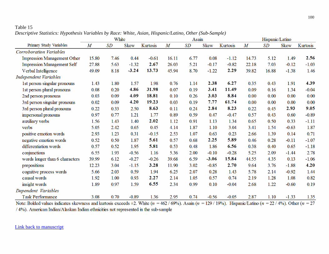
100

Table 15

Descriptive Statistics: Hypothesis Variables by Race: White, Asian, Hispanic/Latino, Other (Sub-Sample)

Link back to manuscript

101

Table 15

Descriptive Statistics: Hypothesis Variables by Race: Black, Hawaiian/Pacific Islander (Sub-Sample) cont’d

Link back to manuscript

Primary Study Variables M SD Skew Kurtosis M SD Skew Kurtosis M SD Skew Kurtosis

Corroboration Variables

Impression Management Other 17.07 7.82 -0.04 -1.33 17.07 8.60 0.70 -0.10 16.00 - - -

Impression Management Self 29.07 4.43 -0.03 -1.32 29.14 5.53 -0.47 -1.56 34.00 - - -

Verbal Intelligence 45.36 9.25 -1.06 0.17 48.71 4.34 0.94 0.93 55.00 - - -

Independent Variables

1st person singular pronouns 0.93 1.48 1.64 1.21 0.43 0.58 1.22 0.31 0.00 - - -

1st person plural pronouns 0.12 0.21 1.59 1.13 0.02 0.07 3.74 14.00 0.00 - - -

2nd person pronouns 0.06 0.15 2.68 6.76 0.02 0.07 3.74 14.00 0.00 - - -

3rd person singular pronouns 0.00 0.00 0.00 0.00 0.02 0.07 3.74 14.00 0.00 - - -

3rd person plural pronouns 0.14 0.15 0.60 -0.73 0.26 0.37 2.22 5.29 0.00 - - -

impersonal pronouns 0.66 0.43 0.21 -0.90 0.68 0.44 1.16 0.85 0.00 - - -

auxiliary verbs 1.33 1.38 2.17 5.98 0.88 0.79 1.57 3.06 0.00 - - -

verbs 5.12 2.42 1.78 4.97 3.65 1.03 0.38 -1.16 0.85 - - -

positive emotion words 2.65 1.48 1.67 3.06 2.62 1.14 -0.20 -0.09 1.71 - - -

negative emotion words 0.51 0.47 0.70 -0.11 0.59 0.38 0.37 0.35 0.00 - - -

differentiation words 0.55 0.44 1.03 0.80 0.50 0.30 0.98 1.76 0.00 - - -

conjunctions 5.61 2.74 0.33 -1.55 6.14 2.09 0.71 0.87 4.27 - - -

words longer than 6 characters 37.17 6.46 0.88 1.26 45.85 5.22 0.40 0.04 52.14 - - -

prepositions 12.03 3.11 2.37 6.71 11.30 3.01 -1.19 1.74 11.11 - - -

cognitive process words 5.21 1.96 -0.08 -1.06 5.17 1.74 0.31 -0.70 1.71 - - -

causal words 1.73 0.89 -0.35 0.00 1.71 0.82 -0.06 -1.06 0.85 - - -

insight words 1.56 0.93 0.74 1.10 1.82 0.75 0.34 -0.50 0.85 - - -

Dependent Variables

Task Performance 3.01 0.80 -0.01 -1.66 3.37 0.51 -0.18 -1.31 3.00 - - -

Hawaiin/Pacific IslanderBlackOther

Note: bolded values indicates skewness and kurtosis exceeds ±2. African American (n = 25 / 4%). American Indian/Alaskan Indian ethnicities not represented in

the sub-sample.

102

Table 16

Descriptive Statistics: Hypothesis Variables by Education: Bachelor’s, Master’s, Some College, Doctorate (Sub-Sample)

Link back to manuscript

Primary Study Variables M SD Skew Kurtosis M SD Skew Kurtosis M SD Skew Kurtosis M SD Skew Kurtosis

Corroboration Variables

Impression Management Other 16.19 7.20 0.20 -0.95 15.16 6.68 0.51 -0.30 17.53 8.56 0.50 -0.64 15.64 7.84 0.25 -1.02

Impression Management Self 27.98 5.17 -0.88 1.11 27.18 5.24 -0.67 0.24 29.11 5.46 -1.37 2.33 27.91 6.93 -1.86 4.73

Verbal Intelligence 47.34 9.60 -2.47 7.24 49.64 6.28 -0.96 0.58 47.56 8.72 -2.99 12.98 49.32 10.07 -2.39 6.68

Independent Variables

1st person singular pronouns 1.17 1.55 1.65 2.18 0.90 1.24 1.86 3.34 1.81 2.00 1.01 -0.08 0.64 1.17 2.82 8.41

1st person plural pronouns 0.07 0.16 3.14 10.83 0.08 0.27 5.20 29.76 0.11 0.22 3.36 14.29 0.04 0.08 2.05 3.27

2nd person pronouns 0.04 0.13 5.50 36.73 0.06 0.15 3.59 15.90 0.03 0.10 4.02 16.50 0.09 0.27 3.38 11.48

3rd person singular pronouns 0.03 0.14 7.95 76.65 0.02 0.06 3.55 11.42 0.03 0.10 3.64 14.01 0.01 0.04 4.69 22.00

3rd person plural pronouns 0.20 0.29 2.17 5.26 0.18 0.33 2.80 9.52 0.30 0.46 2.74 9.50 0.10 0.15 1.76 3.26

impersonal pronouns 0.95 0.67 1.08 1.46 0.79 0.65 1.79 6.01 1.23 0.88 0.67 -0.21 0.50 0.54 1.50 1.88

auxiliary verbs 1.40 1.20 1.36 1.93 1.21 1.07 1.68 3.59 2.23 1.90 1.12 1.21 0.79 1.00 2.60 8.65

verbs 4.91 2.18 0.84 0.77 4.38 2.12 1.45 3.80 5.92 2.43 0.90 0.79 3.04 1.97 0.63 0.89

positive emotion words 2.96 1.18 0.46 -0.22 2.40 0.93 0.39 -0.01 3.43 1.08 0.03 -0.40 1.96 1.05 0.18 -1.49

negative emotion words 0.51 0.45 1.48 2.69 0.52 0.65 2.99 10.93 0.62 0.46 0.60 -0.25 0.44 0.59 2.29 6.40

differentiation words 0.55 0.45 1.66 5.33 0.54 0.56 2.58 9.91 0.74 0.60 0.86 0.86 0.33 0.35 1.69 2.52

conjunctions 6.49 1.91 -0.11 0.27 5.80 2.00 -0.14 0.22 6.85 1.61 -0.50 0.87 5.50 2.44 -0.52 -0.39

words longer than 6 characters 39.87 5.83 -0.11 -0.19 41.88 5.30 -0.50 -0.32 38.29 7.18 0.05 0.26 40.24 9.92 -2.85 10.86

prepositions 12.20 2.75 -0.51 1.80 11.92 3.17 -1.13 2.85 12.87 2.60 -0.51 0.79 11.31 3.14 -2.22 7.71

cognitive process words 5.95 2.05 0.77 2.24 5.71 1.84 -0.26 0.63 6.17 2.10 0.41 -0.38 4.27 2.01 0.07 0.46

causal words 2.08 1.08 0.90 2.04 1.95 0.94 0.58 0.73 1.85 0.84 0.90 0.09 1.40 0.88 0.72 0.73

insight words 2.02 1.03 1.57 6.24 2.10 0.91 0.75 0.97 1.92 0.90 0.75 1.74 1.69 1.11 0.68 0.43

Dependent Variables

Task Performance 3.07 0.74 -0.92 1.47 3.05 0.68 -0.98 0.88 3.13 0.78 -0.83 0.14 2.99 0.75 -1.29 3.74

Note: Bolded values indicate skewness and kurtosis exceeds ±2. Bachelors (n = 325 / 49%). Masters (n = 122 / 18%). Some College (n = 83 / 12%). Doctorate (n = 27 / 4%).

Bachelors Masters Some College Doctorate

103

Table 16

Descriptive Statistics: Hypothesis Variables by Education Professional, Associates, High School, Trade/Vocational/Technical (Sub-Sample) Cont’d

Link back to manuscript

Primary Study Variables M SD Skew Kurtosis M SD Skew Kurtosis M SD Skew Kurtosis M SD Skew Kurtosis

Corroboration Variables

Impression Management Other 14.22 6.03 -0.09 -1.24 15.73 8.68 0.77 -1.06 15.73 8.68 0.77 -1.06 18.18 8.53 0.56 -0.47

Impression Management Self 22.67 6.56 -0.23 -0.40 25.18 7.04 -1.35 3.08 25.18 7.04 -1.35 3.08 28.88 4.86 -1.01 1.79

Verbal Intelligence 44.94 12.82 -2.37 7.29 50.73 3.20 0.98 0.90 50.73 3.20 0.98 0.90 49.59 2.81 -0.13 -0.21

Independent Variables

1st person singular pronouns 1.51 2.32 2.24 4.84 0.78 0.90 1.25 0.96 0.78 0.90 1.25 0.96 2.48 2.76 0.97 -0.45

1st person plural pronouns 0.08 0.23 2.78 7.07 0.13 0.22 2.17 5.10 0.13 0.22 2.17 5.10 0.09 0.18 2.26 4.42

2nd person pronouns 0.02 0.07 3.16 9.84 0.03 0.10 3.32 11.00 0.03 0.10 3.32 11.00 0.02 0.05 3.26 10.74

3rd person singular pronouns 0.02 0.04 2.78 6.59 0.02 0.08 3.32 11.00 0.02 0.08 3.32 11.00 0.03 0.07 2.25 3.85

3rd person plural pronouns 0.09 0.19 1.80 2.03 0.24 0.38 1.27 -0.07 0.24 0.38 1.27 -0.07 0.18 0.18 0.64 -0.53

impersonal pronouns 0.73 0.61 0.54 -0.96 1.19 0.80 0.68 0.56 1.19 0.80 0.68 0.56 1.15 1.04 1.55 2.63

auxiliary verbs 1.10 1.33 1.93 4.23 1.16 1.23 2.46 7.18 1.16 1.23 2.46 7.18 2.03 1.56 0.97 0.62

verbs 4.07 2.52 0.61 0.88 3.74 2.40 1.23 1.31 3.74 2.40 1.23 1.31 6.02 2.49 0.06 -0.23

positive emotion words 2.33 1.26 -0.10 -0.73 2.56 1.14 -0.79 0.11 2.56 1.14 -0.79 0.11 3.72 1.57 -0.21 0.25

negative emotion words 0.51 0.60 2.05 5.13 0.58 0.73 2.33 6.49 0.58 0.73 2.33 6.49 0.55 0.52 0.77 -0.13

differentiation words 0.33 0.30 0.97 0.42 0.54 0.41 0.72 -0.72 0.54 0.41 0.72 -0.72 0.64 0.64 2.16 5.42

conjunctions 4.89 2.74 -0.44 -0.87 5.35 2.52 -0.37 1.77 5.35 2.52 -0.37 1.77 6.94 1.61 -1.21 1.73

words longer than 6 characters 40.13 6.80 -0.61 0.84 43.43 5.56 -0.77 0.01 43.43 5.56 -0.77 0.01 37.78 5.62 -0.66 -0.55

prepositions 11.48 4.99 -1.02 2.48 10.44 4.28 -1.31 3.43 10.44 4.28 -1.31 3.43 11.96 3.29 -0.82 1.05

cognitive process words 4.79 1.89 -0.68 -0.06 5.29 2.42 0.84 0.53 5.29 2.42 0.84 0.53 5.95 1.95 1.56 5.64

causal words 1.65 0.79 -0.27 0.12 2.09 1.35 0.85 0.51 2.09 1.35 0.85 0.51 1.74 0.87 -0.51 -0.66

insight words 2.01 0.93 0.11 -0.33 1.51 1.04 1.74 4.32 1.51 1.04 1.74 4.32 2.02 1.08 0.38 -0.08

Dependent Variables

Task Performance 2.78 0.66 -0.18 -0.25 3.04 0.77 -1.28 2.56 3.04 0.77 -1.28 2.56 3.15 0.61 -0.27 -0.55

Note: Bolded values indicate skewness and kurtosis exceeds ±2. Professional (n = 28 / 4%). Associates (n = 32 / 5%). High School (n = 25 / 4%). Trade, Vocational, or Technical (n = 25 / 4%).

Trade, Vocational, or TechnicalProfessional Associates High School

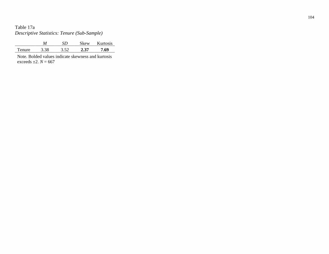
104

Table 17a

Descriptive Statistics: Tenure (Sub-Sample)

M SD Skew Kurtosis

Tenure 3.38 3.52 2.37 7.69

Note. Bolded values indicate skewness and kurtosis

exceeds ±2. N = 667

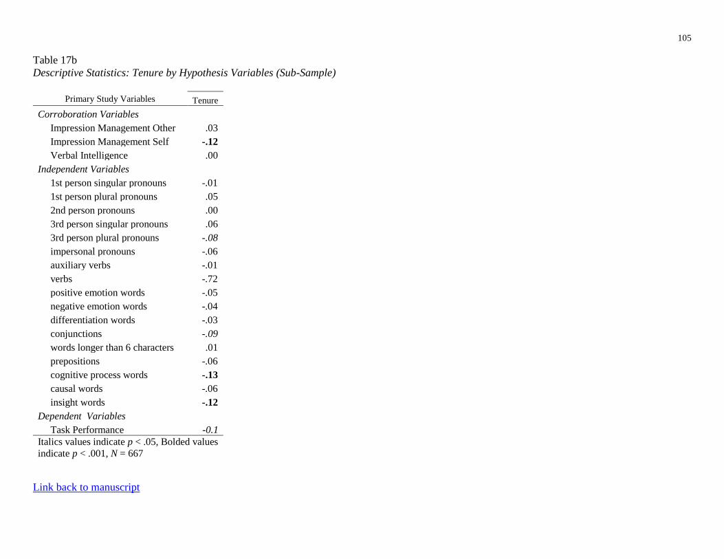
105

Table 17b

Descriptive Statistics: Tenure by Hypothesis Variables (Sub-Sample)

Primary Study Variables Tenure

Corroboration Variables

Impression Management Other .03

Impression Management Self -.12

Verbal Intelligence .00

Independent Variables

1st person singular pronouns -.01

1st person plural pronouns .05

2nd person pronouns .00

3rd person singular pronouns .06

3rd person plural pronouns -.08

impersonal pronouns -.06

auxiliary verbs -.01

verbs -.72

positive emotion words -.05

negative emotion words -.04

differentiation words -.03

conjunctions -.09

words longer than 6 characters .01

prepositions -.06

cognitive process words -.13

causal words -.06

insight words -.12

Dependent Variables

Task Performance -0.1

Italics values indicate p < .05, Bolded values

indicate p < .001, N = 667

Link back to manuscript

106

Table 18

Results of t-Test and Descriptive Statistics for Task Performance by Sex

Link back to manuscript

M SD n M SD n t df

Task Performance 2.91 0.748 407 3.15 0.666 260 -4.14* 665-0.347, -0.124

* p < .001. Males coded as 0 and females as 1

Male

Sex

Female

95% CI for Mean

Difference

107

Table 19

Omnibus ANOVA Results for Task Performance by Race

Link back to manuscript

Sum of Squares df Mean Square F

Between Groups 5.56 6 0.93 1.77

Within Groups 345.30’ 660 0.52

Total 350.87’ 666

p = .102

108

Table 20

Omnibus ANOVA Results for Task Performance by Education

Sum of Squares df Mean Square F

Between Groups 1.85 7 0.26 0.50

Within Groups 349.02" 659 0.53

Total 350.87" 666

p = .836

Link back to manuscript

109

Table 21

Correlation Matrix of All Study Variables and Control Variables

bivariates for

manuscript_30Jan17.xlsx

Link back to manuscript

Age Gender Race Education Tenure Salary Impression

Management - Other

Impression

Management - Self

Task

Performance

Contextual

Performance

Counterproductive

Work Behaviors

Cognitive

Ability

Words Longer

Than 6 Characters

Pronouns Personal

Pronouns

1st Person

Pronouns

1st Person Plural

Pronouns

2nd Person

Pronouns

3rd Person

Singular Pronouns

3rd Person Plural

Pronouns

Impersonal

Pronouns

Prepositions Conjunctions Verbs Positive

Emotion Words

Negative

Emotion Words

Cognitive

Process Words

Insight

Words

Causal

Words

Auxilary

Verbs

Differentiation

Words

Age

Gender .061

Race .105** .243**

Education .107** -.027 -.150**

Tenure .505** -.041 .020 .037

Salary .192** -.034 .005 .188** .199**

Impression Management - Other -.098** -.009 -.072* .030 .034 .039

Impression Management - Self -.147** .134** .099** -.045 -.143** .066 .279**

Task Performance -.042 .161** .100** .012 -.090* -.015 .090* .367**

Contextual Performance -.004 .126** .053 .074* .005 .072* .291** .319** .557**

Counterproductive Work Behaviors -.125** -.116** -.107** .098** .026 -.073* .315** -.043 -.124** .039

Cognitive Ability .131** .167** .229** -.094** -.015 .015 -.160** .106** .165** .034 -.159**

Words Longer Than 6 Characters .047 .189** .254** -.085* -.040 .014 -.172** .105** .145** .056 -.221** .285**

Pronouns .025 .105** .176** -.118** -.023 -.094** .038 .037 .048 .012 -.037 .070* -.142**

Personal Pronouns .045 .106** .152** -.105** .003 -.091** .052 .020 .037 .008 -.012 .045 -.204** .957**

1st Person Pronouns .041 .085* .144** -.094** .007 -.088* .065 .017 .031 .003 .000 .019 -.214** .923** .973**

1st Person Plural Pronouns .065 .031 .067 -.040 .034 .021 -.014 -.071* -.034 .016 -.026 .042 -.038 .255** .250** .132**

2nd Person Pronouns .006 -.028 -.039 .020 -.006 -.075* -.002 .016 .021 -.015 .017 .026 -.043 .200** .214** .117** -.008

3rd Person Singular Pronouns .046 .049 .030 -.024 .053 -.012 -.037 .022 .062 -.019 -.076* .060 .024 .100** .092** .049 -.001 -.003

3rd Person Plural Pronouns -.006 .167** .114** -.106** -.053 -.032 -.021 .055 .044 .038 -.042 .108** -.022 .450** .432** .274** .169** .006 .035

Impersonal Pronouns -.033 .063 .168** -.102** -.077* -.066 -.010 .065 .055 .016 -.083* .104** .057 .732** .504** .465** .173** .092** .083* .328**

Prepositions .070* .185** .223** -.028 -.062 .027 -.113** .130** .162** .098** -.160** .200** .366** .334** .274** .235** .146** .014 .060 .257** .356**

Conjunctions .061 .216** .275** -.130** -.094** .008 -.081* .172** .190** .098** -.190** .278** .408** .310** .251** .215** .126** .000 .116** .238** .338** .652**

Verbs .077* .094** .166** -.076* .007 -.063 .053 .080* .038 .039 .001 .056 -.098** .575** .553** .535** .145** .050 .065 .293** .418** .363** .301**

Positive Emotion Words -.053 .126** .167** -.144** -.058 -.042 .002 .097** .123** .064 -.088* .150** .225** .335** .285** .271** .040 .048 .030 .182** .331** .439** .453** .299**

Negative Emotion Words -.001 -.003 .045 -.048 -.051 .017 -.081* .063 .086* .084* -.121** .076* .235** .073* .029 .018 -.042 .046 .024 .063 .152** .224** .238** .074* .227**

Cognitive Process Words -.053 .143** .182** -.136** -.140** -.023 -.051 .165** .165** .092** -.168** .190** .404** .311** .209** .163** .133** .092** .030 .221** .436** .542** .546** .303** .464** .355**

Insight Words -.072* .047 .024 -.028 -.131** .002 -.044 .100** .094** .030 -.077* .064 .390** .152** .075* .058 .020 .028 .019 .103** .276** .383** .338** .118** .357** .362** .780**

Causal Words .002 .070* .193** -.082* -.078* .024 -.127** .119** .130** .062 -.184** .199** .355** .114** .038 .009 .122** -.008 .019 .105** .252** .432** .454** .188** .297** .218** .747** .442**

Auxilary Verbs .052 .079* .129** -.067 .056 -.095** .055 .054 .025 .034 -.001 .031 -.190** .701** .695** .689** .156** .061 .093** .293** .456** .222** .205** .666** .224** .011 .193** .025 .038

Differentiation Words -.018 .122** .113** -.128** -.045 -.054 .034 .078* .076* .030 -.076* .094** .087* .313** .233** .183** .118** .228** .018 .182** .387** .231** .294** .198** .220** .119** .476** .230** .158** .191**

* p < .05, **p < .001, N = 809

110

Table 22

Test for Normality for Predictor Variables

Kolmogorov-Smirnov Test Shapiro-Wilk Test

Primary Study Variables D df p D df p

Independent Variables

1st person singular pronouns .337 847 p < .001 .426 847 p < .001

1st person plural pronouns .470 847 p < .001 .309 847 p < .001

2nd person pronouns .457 847 p < .001 .076 847 p < .001

3rd person singular pronouns .506 847 p < .001 .091 847 p < .001

3rd person plural pronouns .396 847 p < .001 .515 847 p < .001

Impersonal pronouns .207 847 p < .001 .787 847 p < .001

Auxiliary verbs .269 847 p < .001 .578 847 p < .001

Verbs .118 847 p < .001 .799 847 p < .001

Positive emotion words .090 847 p < .001 .937 847 p < .001

Negative emotion words .310 847 p < .001 .413 847 p < .001

Differentiation words .325 847 p < .001 .359 847 p < .001

Conjunctions .111 847 p < .001 .943 847 p < .001

Words longer than 6 characters .137 847 p < .001 .904 847 p < .001

Prepositions .119 847 p < .001 .912 847 p < .001

Cognitive process words .076 847 p < .001 .882 847 p < .001

Causal words .117 847 p < .001 .924 847 p < .001

Insight words .130 847 p < .001 .825 847 p < .001

Link back to manuscript

111

Table 23

Descriptive Statistics: LIWC Categories for Hypothesis 2-5 with Base Rate Comparisons (Full Sample)

LIWC categories for hypothesis 2-5 M SD Skew Kurtosis

1st person singular pronouns 0.94 (4.99) 1.60 (2.46) 2.25 5.18

1st person plural pronouns 0.05 (0.72) 0.18 (0.83) 5.59 39.55

2nd person pronouns 0.04 (1.70) 0.19 (1.35) 7.23 62.76

3rd person singular pronouns 0.01 (1.88) 0.08 (1.53) 12.32 208.80

3rd person plural pronouns 0.13 (0.66) 0.29 (0.60) 3.31 14.02

Impersonal pronouns 0.67 (5.26) 0.74 (1.62) 1.37 2.05

Auxiliary verbs 1.18 (8.53) 1.50 (2.04) 2.44 9.93

Verbs 4.24 (16.44) 2.99 (2.93) 1.45 6.58

Positive emotion words 2.39 (3.67) 1.73 (1.63) 0.91 2.58

Negative emotion words 0.43 (1.84) 0.62 (1.09) 2.97 14.13

Differentiation words 0.44 (2.99) 0.59 (1.18) 3.47 26.80

Conjunctions 4.94 (5.90) 2.91 (1.57) -0.30 -0.75

Words longer than 6 characters 38.30 (15.60) 10.81 (3.76) -1.20 2.14

Prepositions 9.97 (12.93) 4.98 (2.11) -0.70 -0.16

Cognitive process words 4.73 (10.61) 2.88 (3.02) 0.26 0.65

Causal words 1.57 (1.40) 1.27 (0.73) 0.82 1.21

Insight words 1.73 (2.16) 1.37 (1.08) 1.24 3.37

Note. Bolded values indicate skewness and kurtosis exceeds ±2. N = 809 Values in parentheses

are LIWC reported average base rates and standard deviations

Link back to manuscript

112

Table 24

Logistic Regression Model for Training Data (n = 462)

95% CI for Odds Ratio

B SE Lower Odds

Ratio

Upper

Included in final training model

Constant -0.02 0.24

Sex 0.67 0.22 1.27 1.95 3.01

Third-person plural pronouns 5.45 3.12 0.51 232.545 105267.46

Impersonal pronouns -0.34 0.19 0.49 0.72 1.04

Auxiliary verbs 0.33 0.12 1.10 1.40 1.77

Adverbs -0.43 0.21 0.44 0.65 0.98

Sadness words 1.69 0.84 1.05 5.43 28.15

Certainty Words 0.30 0.17 0.96 1.35 1.90

Nonfluencies 0.79 0.46 0.90 2.21 5.43

Colon -0.10 0.04 0.83 0.91 0.99

Dash -0.04 0.02 0.93 0.97 1.00

Parentheses 0.13 0.04 1.05 1.14 1.24

Note. R2 = .09 (Hosmer & Lemeshow), .12 (Cox & Snell), .16 (Nagelkerke). Model χ2 =

57.48, p < .001. Bolded odds ratios numbers indicate that coefficient doesn't cross 1,

suggesting a significant predictor in logistics regression equation. Training model

sample size n = 462

Link back to manuscript

113

Table 25

Logistic Regression Model for Testing Data (n = 205)

95% CI for Odds Ratio

B SE Lower Odds Ratio Upper

Included in final testing

model

Constant 0.67 0.41

Sex 0.45 0.33 0.82 1.57 3.00

3rd person plural pronouns -1.08 3.55 0.00 0.34 356.20'

Impersonal pronouns -0.22 0.26 0.48 0.80 1.33

Auxiliary verbs -0.40 0.16 0.49 0.67 0.91

Adverbs 0.61 0.29 1.05 1.84 3.24

Sadness words 2.41 1.25 0.96 11.14 128.83'

Certainty Words -0.03 0.27 0.57 0.97 1.64

Nonfluencies 0.22 0.70 0.31 1.25 4.94

Colon -0.12 0.07 0.78 0.89 1.02

Dash 0.10 0.06 0.97 1.10 1.25

Parentheses -0.14 0.08 0.75 0.87 1.01

Note. R2 = .10 (Hosmer & Lemeshow), .12 (Cox & Snell), .16 (Nagelkerke). Model

χ2 = 13.12, p = .041. Bolded odds ratios numbers indicate that coefficient doesn't

cross 1, suggesting a significant predictor in logistics regression equation. Testing

model sample size n= 205

Link back to manuscript

114

Table 26

Testing for Significant Differences in B-weights from Training to Test Models

B (training

model)

B (testing model) t p

Comparison B weights

Sex 0.67 0.45 0.55 0.58

3rd person plural pronouns 5.45 -1.08 1.38 0.17

Impersonal pronouns -0.34 -0.22 0.35 0.72

Auxiliary verbs 0.33 -0.40 3.74 0.00

Adverbs -0.43 0.61 2.94 0.00

Sadness words 1.69 2.41 0.48 0.63

Certainty words 0.30 -0.03 1.04 0.30

Nonfluencies 0.79 0.22 0.68 0.49

Colon -0.10 -0.12 0.24 0.81

Dash -0.04 0.10 2.16 0.03

Parentheses 0.13 -0.14 3.00 0.00

Note. See Soper (2016) and Cohen, Cohen, West, & Aiken (2003) for how to tell

significance. Bolded p-values indicate predictors are retaining significance from

training to testing model tests. Predictors are considered to be still significant if

the p value is above .05

Link back to manuscript

115

Table 27

Pronouns Correlated with Impression Management

Hypothesis 2b

1st person

singular

pronouns

1st person

plural pronouns

2nd person

pronouns

3rd person

singular

pronouns

3rd person

plural pronouns

Impersonal

pronouns

Impression Management Self .02 -.07 .02 .02 .06 .07

Impression Management Other .07 -.01 .00 -.04 -.02 -.01

Note. Bolded values indicate correlations that were significant at p < .05. N = 809

Link back to manuscript

116

Table 28

Task Performance Regressed on Pronouns

Variables R R2 ΔR2 B SEB sr2

Step 1 - control variables .178 .032 .032**

Sex 0.231** 0.057 0.156 .024

Tenure -0.017*ff 0.008 -0.081 .007

Step 2 - log-transformed pronoun predictors .205 .042 .010

Sex 0.22** 0.058 0.148 .021

Tenure -0.018*f 0.008 -0.087 .007

Pronouns

1st person singular pronouns 0.097 0.127 0.034 .001

1st person plural pronouns -0.666 0.470 -0.055 .003

2nd person pronouns -0.021 0.550 -0.001 .000

3rd person singular pronouns 1.868 1.042 0.069 .005

3rd person plural pronouns 0.108 0.337 0.013 .000

Impersonal pronouns -0.279f 0.203 -0.063 .003

Note. All predictors were log-transformed. Sex was a dichotomous variable with males coded as 0 and females as 1.

* p < .05. ** p < .001.

Link back to manuscript

117

Table 29

Task Performance Regressed on Verbs

Variables R R2 ΔR2 B SEB sr2

Step 1 - control variables .178 .032 .032**

Sex 0.231** 0.057 0.156 .024

Tenure -0.017*ff 0.008 -0.081 .007

Step 2 - log-transformed verb predictors .178 .032 .000

Sex f0.230** 0.057 0.155 .024

Tenure -0.017*j 0.008 -0.080 .006

Verbs 0.029j 0.126 0.009 .000

Note. All predictors were log-transformed. Sex was a dichotomous variable with males coded as 0 and females as 1.

* p < .05, ** p < .001.

Link back to manuscript

118

Table 30

Task Performance Regressed on Positive Emotion Words

Variables R R2 ΔR2 B SEB sr2

Step 1 - control variables .178 .032 .032**

Sex 0.231** 0.057 0.156 .024

Tenure -0.017*jj 0.008 -0.081f .007

Step 2 - log-transformed positive emotion words .181 .033 .001jjj

Sex 0.228** 0.057 0.154 .023

Tenure -0.016*jj 0.008 -0.079f .006

Positive emotion words 0.123ff 0.152 0.031 .001

Note. All predictors were log-transformed. Sex was a dichotomous variable with males coded as 0 and females as 1.

* p < .05. ** p < .001.

Link back to manuscript

119

Table 31

Contextual Performance Regressed on Positive Emotion Words

Variables R R2 ΔR2 B SEB sr2

Step 1 - control variable .126 .016 .016**

Sex 0.197** 0.060 0.126 .016

Step 2 - log-transformed positive emotion words .183 .033 .000ff

Sex 0.195** 0.060 0.125 .015

Positive emotion words 0.075fff 0.161 0.018 .000

Note. All predictors were log-transformed. Sex was a dichotomous variable with males coded as 0 and females as 1.

** p < .01.

Link back to manuscript

120

Table 32

Counterproductive Job Performance Regressed on Negative Emotion Words

Variables R R2 ΔR2 SE B sr2 p

Negative emotion words .062 .004 .004 -0.416 0.258 -0.062 .004 .11

Note. All predictors were log-transformed.

Link back to manuscript

121

Table 33

Task Performance Regressed on Negative Emotion Words

Variables R R2 ΔR2 B SE B sr2 p

Negative emotion words .029 .001 .001 0.037 0.505 0.029 .001 .16

Note. All predictors were log-transformed.

Link back to manuscript

122

Table 34

Verbal Intelligence Correlated with Differentiation Words, Conjunctions, and Words Longer than Six Characters, Prepositions, Cognitive Process

Words, Causal Words, and Insight Words

Hypothesis 4a-g Differentiation

Words

Conjunctions Words longer than

6 characters

Prepositions Cognitive

Process Words

Causal

Words

Insight

Words

Verbal Intelligence .094 .278 .285 .200 .190 .199 .064

Note. Bolded values indicate correlations that were significant at p < .001. Italics indicate correlations that were significant at p <

.05. N = 809

Link back to manuscript

123

Table 35

Task Performance Regressed on Differentiation Words, Conjunctions, and Words Longer than Six Characters, Prepositions, Cognitive Process

Words, Causal Words, and Insight Words

Variables R R2 ΔR2 B SE B sr2

Step 1 - control variables .178 .032 .032**

Sex 0.231**’ 0.057 0.156 .024

Tenure -0.017** 0.008 -0.081 .007

Step 2 - log transformed verbal intelligence

proxy predictors .215 .046 .015**

Sex 0.218**’ 0.058 0.147 .022

Tenure -0.015** 0.008 -0.073 .005

Verbal Intelligence proxy predictors

differentiation words -0.359’ 0.251 -0.066 .004

conjunctions 0.027 0.014 ’0.087 .008

words longer than 6 characters -0.024 0.283 -0.003 .000

prepositions -0.172 0.165 -0.052 .003

cognitive process words 0.606 0.360 ’0.163 .027

insight words -0.480 0.252 -0.117 .014

causal words -0.058 0.235 -0.015 .000

Note: Sex was a dichotomous variable with males coded as 0 and females as 1.*p < .05. ** p < .001.

Link back to manuscript

124

Table 36

Task Performance Regressed on Cognitive Ability and the Written Cognitive Ability Index

Variables R R2 ΔR2 B SE B sr2

Step 1 - control variable .161 .026 .026**

Sex 0.258** .056 .161 .026

Step 2 - cognitive ability and WCAI

text analytics composite variable .256 .065 .040**

Sex 0.176** .057 .109 .012

Cognitive ability 0.007** .002 .102 .010

WCAI 0.030** .007 .150 .023

Note. * p < .005, ** p < .001. Sex was a dichotomous variable with males coded as 0 and females as 1.

Link back to manuscript

125

Figure 1. The frequency of first-person singular pronoun usage in aggregate resume text.

126

Figure 2. The frequency of first-person plural pronoun usage in aggregate resume text.

127

Figure 3. The frequency of second-person pronoun usage in aggregate resume text.

128

Figure 4. The frequency of third-person singular pronoun usage in aggregate resume text.

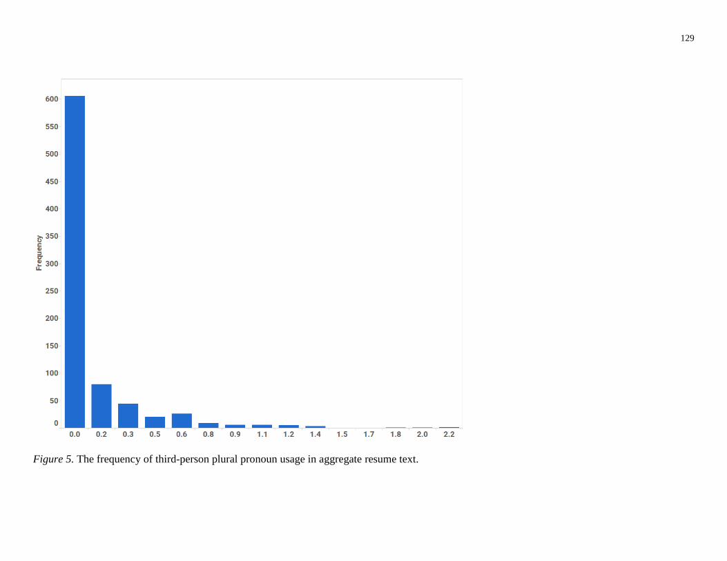
129

Figure 5. The frequency of third-person plural pronoun usage in aggregate resume text.

130

Figure 6. The frequency of impersonal pronoun usage in aggregate resume text.

131

Figure 7. The frequency of verb usage in aggregate resume text.

Link back to manuscript

132

Figure 8. The frequency of positive emotion word usage in aggregate resume text.

Link back to manuscript

133

Figure 9. The frequency of negative emotion word usage in aggregate resume text.

Link back to manuscript

134

Figure 10. The frequency of differentiation word usage in aggregate resume text.

135

Figure 11. The frequency of conjunction usage in aggregate resume text.

136

Figure 12. The frequency of words longer than six characters in aggregate resume text.

137

Figure 13. The frequency of preposition usage in aggregate resume text.

138

Figure 14. The frequency of cognitive process words in aggregate resume text.

139

Appendix A

LIWC Word Categories and Example Word for Each Category

140

141

142

Appendix B

Decision Rules for Selecting Independent Variables and LIWC Categories

LIWC word categories were hierarchical in nature, with higher order categories representing a

combination of lower order categories. For example, cognitive processes, a category which

focused on word markers of cognitive activity (Pennebaker, 2015), is an aggregate measure of

the cognitive process sub-categories of insight, causation, discrepancy, tentativeness, certainty,

and differentiation. This approach has only recently been clarified in the latest LIWC manual

(Pennebaker, 2015). The prior documentation suggested higher order categories but did not

indicate that the higher order categories were created by summing the lower level categories.

This is problematic for hypotheses that posit a linear model that includes both higher and

lower order word categories (e.g. the cognitive process category and the causal category)

because the inclusion of these categories introduces a high degree of multicollinearity. This

makes a test of a linear or curvilinear relationship untenable. Additional categories increase the

predictor to sample size ratio, decreasing power, and degrees of freedom. Therefore, business

rules were developed when deciding whether to use the higher order or lower order categories.

They are described below as follows.

1) If the lower order categories (e.g. insight, causation, discrepancy) have a correlation that

exceeds |r = .65|, use the higher order category, e.g. cognitive process. Otherwise, use the

lower order categories.

2) Lower order categories are preferred to higher order categories due to greater explanatory

capability and theory building. For example, it is preferable to discuss how first-person

pronouns drive job performance rather than pronouns.

These business rules applied to all hypotheses in this study. However, it should be noted

143

that these decisions resulted in what initially appeared to be a random assortment of predictors

for job performance (Hypothesis 1). However, this is not the case for the following reasons.

First, understanding the bivariate correlations between lower and higher order word categories is

standard practice. Redundant predictors are often collapsed into a single predictor. Second, while

one would prefer greater precision in an applied context, a more robust regression model is

preferred to a brittle model. That is to say, the inclusion of terms with multicollinearity not only

represents an incorrectly specified model but also adds unnecessary complexity, violating the

principle of parsimony. Thus, parsimony and a correctly specified model are more important in

practice than extreme precision. Finally, given the small sample size (N = 393), using higher

order categories aided in dimensionality reduction of the predictor space.

Correlation

matrices checking to lower order categories for redundancy with higher order category_02Feb17.xlsx

144

Appendix C

Validity Evidence for the Spot-The-Word Test

The Spot-The-Word test has strong convergent validity with established measures of

verbal intelligence, including (a) the National Adult Reading Test, (r = 0.83 with Form A; r =

0.86 with Form B; Baddeley et al., 1993), (b) the American National Adult Reading Test (r =

0.56; Yuspeh & Vanderploeg, 2000), (c) the Wechsler Adult Intelligence Scale-Revised

Vocabulary subtest (r = 0.58; Yuspeh & Vanderploeg), and (d) the Shipley Institute of Living

Scale Vocabulary subtest (r = 0.66; Yuspeh & Vanderploeg). In addition, the STW has strong

alternate forms reliability (r = 0.88, Baddeley, et al., 1993). Finally, the STW has also shown to

be an adequate measure of general intelligence; Yuspeh and Vanderploeg reported a validity

coefficient of 0.35 between the STW and the Wechsler Adult Intelligence Scale.

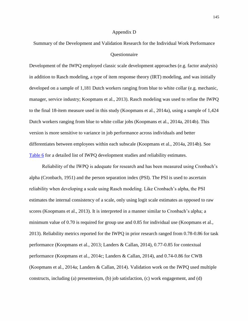
145

Appendix D

Summary of the Development and Validation Research for the Individual Work Performance

Questionnaire

Development of the IWPQ employed classic scale development approaches (e.g. factor analysis)

in addition to Rasch modeling, a type of item response theory (IRT) modeling, and was initially

developed on a sample of 1,181 Dutch workers ranging from blue to white collar (e.g. mechanic,

manager, service industry; Koopmans et al., 2013). Rasch modeling was used to refine the IWPQ

to the final 18-item measure used in this study (Koopmans et al., 2014a), using a sample of 1,424

Dutch workers ranging from blue to white collar jobs (Koopmans et al., 2014a, 2014b). This

version is more sensitive to variance in job performance across individuals and better

differentiates between employees within each subscale (Koopmans et al., 2014a, 2014b). See

Table 6 for a detailed list of IWPQ development studies and reliability estimates.

Reliability of the IWPQ is adequate for research and has been measured using Cronbach’s

alpha (Cronbach, 1951) and the person separation index (PSI). The PSI is used to ascertain

reliability when developing a scale using Rasch modeling. Like Cronbach’s alpha, the PSI

estimates the internal consistency of a scale, only using logit scale estimates as opposed to raw

scores (Koopmans et al., 2013). It is interpreted in a manner similar to Cronbach’s alpha; a

minimum value of 0.70 is required for group use and 0.85 for individual use (Koopmans et al.,

2013). Reliability metrics reported for the IWPQ in prior research ranged from 0.78-0.86 for task

performance (Koopmans et al., 2013; Landers & Callan, 2014), 0.77-0.85 for contextual

performance (Koopmans et al., 2014c; Landers & Callan, 2014), and 0.74-0.86 for CWB

(Koopmans et al., 2014a; Landers & Callan, 2014). Validation work on the IWPQ used multiple

constructs, including (a) presenteeism, (b) job satisfaction, (c) work engagement, and (d)

146

manager ratings of performance. See Table 6 for a detailed list of IWPQ validation studies and

corresponding validity coefficients.

Respondents were asked to recall their job performance behaviors from the past three

months and respond to Likert-scaled items ranging from 0 (seldom/never) to 4 (always/often).

Mean scores were obtained for each sub-scale by summing the item scores and dividing the total

by the number of items in that particular subscale. This resulted in a sub-scale score with a range

of 0 to 4. Higher scores reflected higher task and contextual performance and higher

counterproductive work behavior. A single overall score was not computed as current job

performance theory conceptualizes job performance as multidimensional (Campbell, 1990, 2012;

Koopmans et al., 2014a). What is more, computing a single overall score would necessarily

include the counterproductive work behavior subscale, and its inclusion would result in sub-

optimal psychometrics due to its negative correlation with the other two sub-scale scores.

147

Appendix E

Sample Output from the LIWC Software

Response_ID Sixltr ppron i we you shehe they ipron article prep auxverb

41194514 31.75 0 0 0 0 0 0 0 2.84 12.32 0.95

41194519 37.16 4.65 3.67 0 0 0.24 0.73 1.47 5.13 15.4 3.67

41194604 32.76 3 3 0 0 0 0 1.71 6.85 11.56 0.86

41194663 38.05 0.13 0 0 0.13 0 0 0.38 3.88 11.26 0.63

41194668 30.89 1.39 0 0 1.09 0.1 0.2 3.27 10.1 14.26 6.14

41194701 42.29 1.49 1.49 0 0 0 0 1 2.49 9.95 1

41194703 33.33 0 0 0 0 0 0 0 0 0 0

41194755 30.57 3.07 1.38 0.77 0 0 0.92 1.84 2.61 7.22 2.61

41194759 43.7 0.42 0.42 0 0 0 0 0.84 3.57 11.34 1.26

41194805 35.81 0.31 0 0 0.31 0 0 0 7.91 13.02 1.09

41194866 41.7 0.36 0.36 0 0 0 0 1.09 5.33 12.85 0.85

41194876 37.01 0.15 0.15 0 0 0 0 0 2.32 13.93 0.15

41194912 43.68 0.18 0 0.18 0 0 0 1.44 2.89 14.62 1.08

41194945 41.78 0 0 0 0 0 0 0.47 0.94 13.62 0.94

41194960 26.15 4.36 2.06 0 0 0 2.29 3.21 8.26 12.61 4.13

41194974 38.15 0 0 0 0 0 0 0.8 4.82 14.06 0.8

41195002 33.76 0.25 0.25 0 0 0 0 0 1.78 0.51 0.76

41195044 41.42 1.72 1.47 0.25 0 0 0 0.49 5.39 16.42 0.74

41195078 50.93 0 0 0 0 0 0 0 1.85 14.81 1.39

148

Appendix F

Python Code for Cleaning Up Survey Data

# -*- coding: utf-8 -*-

"""

Created on Thu Dec 17 16:28:00 2015

"""

'''

IMPORT AND CONCATENATE/UNION ALL 5 EXCEL FILES IMPORT AND

CONCATENATE/UNION ALL 5 EXCEL FILES

IMPORT AND CONCATENATE/UNION ALL 5 EXCEL FILES IMPORT AND

CONCATENATE/UNION ALL 5 EXCEL FILES

IMPORT AND CONCATENATE/UNION ALL 5 EXCEL FILES IMPORT AND

CONCATENATE/UNION ALL 5 EXCEL FILES

note: the raw CSV files had the following edits done to them

1) removed first 3 rows that included download and metadata information

(this was included from the survey platform)

2) moved all header columns to a single row, the header column was two rows

3) item column headers had sequential numbers appended to them (e.g.

"15 - Job Performance1", "15 - Job Performance2") this was done as a

precautionary step to ensure that the columns would concatenate/union

all correctly using the for loop

'''

#import required packages and set parameters for creating data visualizations and set

visualization style color

import glob

import pandas as pd

import numpy as np

import seaborn as sns

import matplotlib.pyplot as plt

plt.rcParams['figure.figsize'] = (10, 8)

plt.rcParams['font.size'] = 14

plt.style.use('bmh')

#verify csv files are showing up

glob.glob('C:/Users/Joshuaw/Documents/PhD_Year_5/Data/Raw_Survey/*.csv')

'''

the code commented out below is code to help check that the

concatenation/union all of the survey files was happening correctly

i.e. making sure columns were being mapped to the correct columns

'''

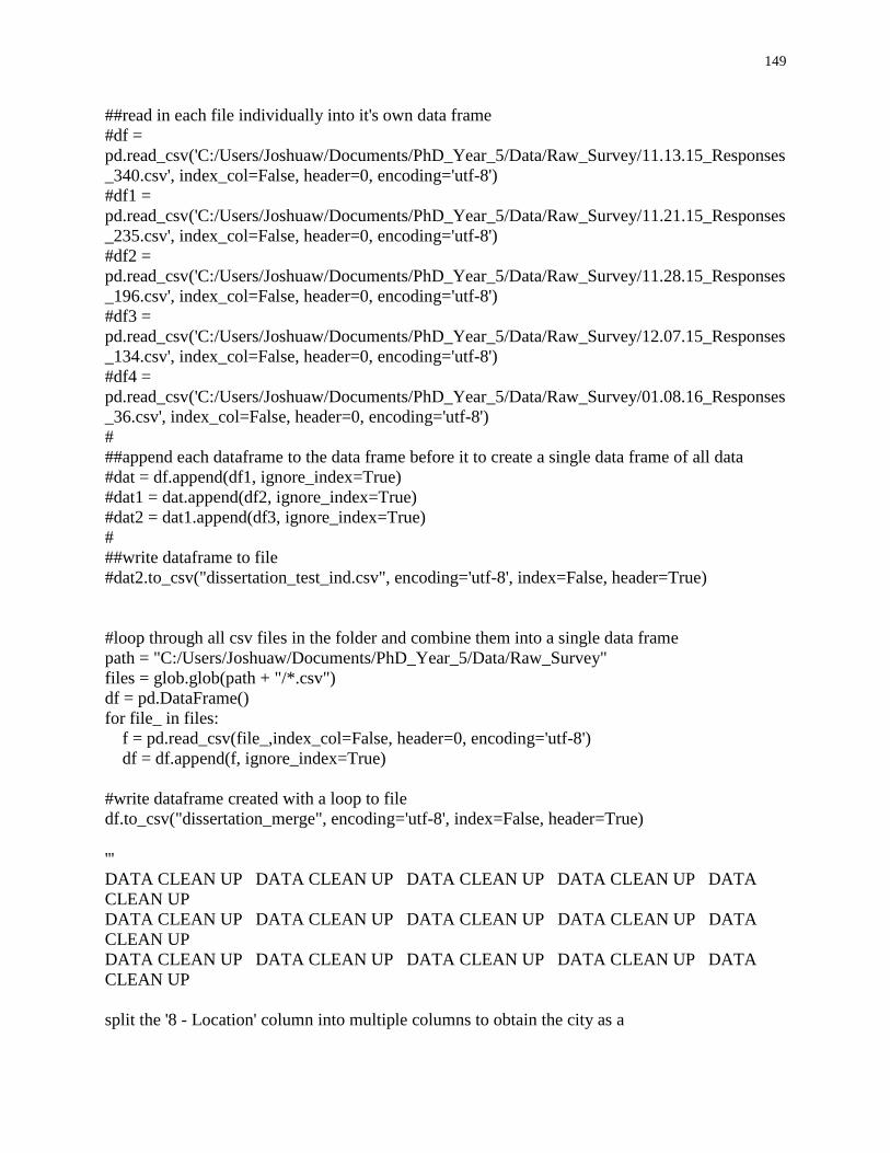
149

##read in each file individually into it's own data frame

#df =

pd.read_csv('C:/Users/Joshuaw/Documents/PhD_Year_5/Data/Raw_Survey/11.13.15_Responses

_340.csv', index_col=False, header=0, encoding='utf-8')

#df1 =

pd.read_csv('C:/Users/Joshuaw/Documents/PhD_Year_5/Data/Raw_Survey/11.21.15_Responses

_235.csv', index_col=False, header=0, encoding='utf-8')

#df2 =

pd.read_csv('C:/Users/Joshuaw/Documents/PhD_Year_5/Data/Raw_Survey/11.28.15_Responses

_196.csv', index_col=False, header=0, encoding='utf-8')

#df3 =

pd.read_csv('C:/Users/Joshuaw/Documents/PhD_Year_5/Data/Raw_Survey/12.07.15_Responses

_134.csv', index_col=False, header=0, encoding='utf-8')

#df4 =

pd.read_csv('C:/Users/Joshuaw/Documents/PhD_Year_5/Data/Raw_Survey/01.08.16_Responses

_36.csv', index_col=False, header=0, encoding='utf-8')

#

##append each dataframe to the data frame before it to create a single data frame of all data

#dat = df.append(df1, ignore_index=True)

#dat1 = dat.append(df2, ignore_index=True)

#dat2 = dat1.append(df3, ignore_index=True)

#

##write dataframe to file

#dat2.to_csv("dissertation_test_ind.csv", encoding='utf-8', index=False, header=True)

#loop through all csv files in the folder and combine them into a single data frame

path = "C:/Users/Joshuaw/Documents/PhD_Year_5/Data/Raw_Survey"

files = glob.glob(path + "/*.csv")

df = pd.DataFrame()

for file_ in files:

f = pd.read_csv(file_,index_col=False, header=0, encoding='utf-8')

df = df.append(f, ignore_index=True)

#write dataframe created with a loop to file

df.to_csv("dissertation_merge", encoding='utf-8', index=False, header=True)

'''

DATA CLEAN UP DATA CLEAN UP DATA CLEAN UP DATA CLEAN UP DATA

CLEAN UP

DATA CLEAN UP DATA CLEAN UP DATA CLEAN UP DATA CLEAN UP DATA

CLEAN UP

DATA CLEAN UP DATA CLEAN UP DATA CLEAN UP DATA CLEAN UP DATA

CLEAN UP

split the '8 - Location' column into multiple columns to obtain the city as a

150

separate column

Note: the split isn't clean, but since we already have a country code all we need is the city for

visualization in Tableau.

'''

s = df['8 - Location'].str.split(',').apply(pd.Series,1)

s.name = '8 - Location' #we need a name to be able to join it to the original dataframe

del df['8 - Location'] #drop the location column

#df1 = df.join(s) #join the 10 columns back to the dataframe

dat = pd.concat([df, s], axis=1)

df = dat #rename the dataframe back to df, for consistency

'''

delete columns: these columns were part of the survey but don't contain

relevant data

'''

df.drop(['Response Status', 'Seq. Number', 'External Reference',

'Respondent Email', 'Email List', '1 - INTRO', '3 - Demographics_header',

'14 - Work_Behavior_Header',

'Spot_The_Word_Test:...........1', 'Spot_The_Word_Test:...........2',

'Spot_The_Word_Test:...........3', 'Spot_The_Word_Test:...........4',

'Spot_The_Word_Test:...........5', 'Spot_The_Word_Test:...........6',

'Spot_The_Word_Test:...........7', 'Spot_The_Word_Test:...........8',

'Spot_The_Word_Test:...........9', 'Spot_The_Word_Test:...........10',

'Spot_The_Word_Test:...........11', 'Spot_The_Word_Test:...........12',

'Spot_The_Word_Test:...........13', 'Spot_The_Word_Test:...........14',

'Spot_The_Word_Test:...........15', 'Spot_The_Word_Test:...........16',

'Spot_The_Word_Test:...........17', 'Spot_The_Word_Test:...........18',

'Spot_The_Word_Test:...........19', 'Spot_The_Word_Test:...........20',

'Spot_The_Word_Test:...........21', 'Spot_The_Word_Test:...........22',

'Spot_The_Word_Test:...........23', 'Spot_The_Word_Test:...........24',

'Spot_The_Word_Test:...........25', 'Spot_The_Word_Test:...........26',

'Spot_The_Word_Test:...........27', 'Spot_The_Word_Test:...........28',

'Spot_The_Word_Test:...........29', 'Spot_The_Word_Test:...........30',

'Spot_The_Word_Test:...........31', 'Spot_The_Word_Test:...........32',

'Spot_The_Word_Test:...........33', 'Spot_The_Word_Test:...........34',

'Spot_The_Word_Test:...........35', 'Spot_The_Word_Test:...........36',

'Spot_The_Word_Test:...........37', 'Spot_The_Word_Test:...........38',

'Spot_The_Word_Test:...........39', 'Spot_The_Word_Test:...........40',

'Spot_The_Word_Test:...........41', 'Spot_The_Word_Test:...........42',

'Spot_The_Word_Test:...........43', 'Spot_The_Word_Test:...........44',

'Spot_The_Word_Test:...........45', 'Spot_The_Word_Test:...........46',

'Spot_The_Word_Test:...........47', 'Spot_The_Word_Test:...........48',

'Spot_The_Word_Test:...........49', 'Spot_The_Word_Test:...........50',

'Spot_The_Word_Test:...........51', 'Spot_The_Word_Test:...........52',

'Spot_The_Word_Test:...........53', 'Spot_The_Word_Test:...........54',

'Spot_The_Word_Test:...........55', 'Spot_The_Word_Test:...........56',

151

'Spot_The_Word_Test:...........57', 'Spot_The_Word_Test:...........58',

'Spot_The_Word_Test:........... 59'], axis =1, inplace=True)

#rename the columns to make them more pythonic and easy to type

#first create a list that contains the new names for the columns

df_cols = ['Response_ID', 'IP_Address', 'Timestamp', 'Device_Data',

'SecondsToComplete', 'Country_Code', 'Region', 'Resume',

'Age', 'Sex', 'Race', 'Education', 'Industry', 'Job_Level',

'Years_Experience', 'Hours_Week', 'Salary', 'Job_Performance1',

'Job_Performance2', 'Job_Performance3', 'Job_Performance4',

'Job_Performance5', 'Job_Performance6', 'Job_Performance7',

'Job_Performance8', 'Job_Performance9', 'Job_Performance10',

'Job_Performance11', 'Job_Performance12', 'Job_Performance13',

'Job_Performance14', 'Job_Performance15', 'Job_Performance16',

'Job_Performance17', 'Job_Performance18', 'Impression_Work1',

'Impression_Work2', 'Impression_Work3', 'Impression_Work4',

'Impression_Work5', 'Impression_Work6', 'Impression_Work7',

'Impression_Work8', 'Impression_Work9', 'Impression_Work10',

'Spot_The_Word_Test:slank', 'Spot_The_Word_Test:chariot',

'Spot_The_Word_Test:lentil', 'Spot_The_Word_Test:glotex',

'Spot_The_Word_Test:stamen', 'Spot_The_Word_Test:dombus',

'Spot_The_Word_Test:loba','Spot_The_Word_Test:comet',

'Spot_The_Word_Test:pylon', 'Spot_The_Word_Test:stroin',

'Spot_The_Word_Test:scrapten', 'Spot_The_Word_Test:flannel',

'Spot_The_Word_Test:fender', 'Spot_The_Word_Test:ullus',

'Spot_The_Word_Test:ragspur', 'Spot_The_Word_Test:joust',

'Spot_The_Word_Test:milliary', 'Spot_The_Word_Test:mantis',

'Spot_The_Word_Test:sterile', 'Spot_The_Word_Test:palth',

'Spot_The_Word_Test:proctive', 'Spot_The_Word_Test:monotheism',

'Spot_The_Word_Test:glivular', 'Spot_The_Word_Test:stallion',

'Spot_The_Word_Test:intervantation', 'Spot_The_Word_Test:rictus',

'Spot_The_Word_Test:byzantine', 'Spot_The_Word_Test:chloriant',

'Spot_The_Word_Test:monologue', 'Spot_The_Word_Test:rufine',

'Spot_The_Word_Test:elegy', 'Spot_The_Word_Test:festant',

'Spot_The_Word_Test:malign', 'Spot_The_Word_Test:vago',

'Spot_The_Word_Test:exonize', 'Spot_The_Word_Test:gelding',

'Spot_The_Word_Test:bulliner', 'Spot_The_Word_Test:trireme',

'Spot_The_Word_Test:visage', 'Spot_The_Word_Test:hyperlisitc',

'Spot_The_Word_Test:froin', 'Spot_The_Word_Test:oratory',

'Spot_The_Word_Test:meridian', 'Spot_The_Word_Test:phillidism',

'Spot_The_Word_Test:grottle', 'Spot_The_Word_Test:strumpet',

'Spot_The_Word_Test:equine', 'Spot_The_Word_Test:psynomy',

'Spot_The_Word_Test:baggalette', 'Spot_The_Word_Test:riposte',

'Spot_The_Word_Test:valance', 'Spot_The_Word_Test:plesmoid',

'Spot_The_Word_Test:introvert', 'Spot_The_Word_Test:vinadism',

'Spot_The_Word_Test:penumbra', 'Spot_The_Word_Test:rubiant',

152

'Spot_The_Word_Test:breen', 'Spot_The_Word_Test:malinger',

'Spot_The_Word_Test:gammon', 'Spot_The_Word_Test:unterried',

'Spot_The_Word_Test:coracle', 'Spot_The_Word_Test:prestasis',

'Spot_The_Word_Test:paramour', 'Spot_The_Word_Test:imbulasm',

'Spot_The_Word_Test:dallow', 'Spot_The_Word_Test:octaroon',

'Spot_The_Word_Test:fleggary', 'Spot_The_Word_Test:carnation',

'Spot_The_Word_Test:liminoid', 'Spot_The_Word_Test:agnostic',

'Spot_The_Word_Test:naquescent', 'Spot_The_Word_Test:plinth',

'Spot_The_Word_Test:thole', 'Spot_The_Word_Test:leptine',

'Spot_The_Word_Test:crattish', 'Spot_The_Word_Test:reform',

'Spot_The_Word_Test:wraith', 'Spot_The_Word_Test:stribble',

'Spot_The_Word_Test:metulate', 'Spot_The_Word_Test:pristine',

'Spot_The_Word_Test:pauper', 'Spot_The_Word_Test:progotic',

'Spot_The_Word_Test:aurant', 'Spot_The_Word_Test:baleen',

'Spot_The_Word_Test:palindrome', 'Spot_The_Word_Test:lentathic',

'Spot_The_Word_Test:hedgehog', 'Spot_The_Word_Test:mordler',

'Spot_The_Word_Test:prassy', 'Spot_The_Word_Test:ferret',

'Spot_The_Word_Test:torbate', 'Spot_The_Word_Test:drumlin',

'Spot_The_Word_Test:texture', 'Spot_The_Word_Test:disenrupted',

'Spot_The_Word_Test:isomorphic', 'Spot_The_Word_Test:thassiary',

'Spot_The_Word_Test:fremoid', 'Spot_The_Word_Test:vitriol',

'Spot_The_Word_Test:farrago', 'Spot_The_Word_Test:gesticity',

'Spot_The_Word_Test:minidyne', 'Spot_The_Word_Test:hermeneutic',

'Spot_The_Word_Test:pusality', 'Spot_The_Word_Test:chaos',

'Spot_The_Word_Test:devastate', 'Spot_The_Word_Test:prallage',

'Spot_The_Word_Test:peremptory', 'Spot_The_Word_Test:paralepsy',

'Spot_The_Word_Test:chalper', 'Spot_The_Word_Test:camera',

'Spot_The_Word_Test:roster', 'Spot_The_Word_Test:fallulate',

'Spot_The_Word_Test:scaline', 'Spot_The_Word_Test:accolade',

'Spot_The_Word_Test:methagenate', 'Spot_The_Word_Test:pleonasm',

'Spot_The_Word_Test:drobble', 'Spot_The_Word_Test:infiltrate',

'Spot_The_Word_Test:mystical', 'Spot_The_Word_Test:harreen',

'Grit1', 'Grit2', 'Grit3', 'Grit4', 'Grit5', 'Grit6', 'Grit7',

'Grit8', 'Location1', 'Location2', 'Location3', 'Location4',

'Location5', 'Location6', 'Location7', 'Location8', 'Location9',

'Location10']

#rename columns using the list that was just created

df.columns = df_cols

'''

RECODE VARIABLES, CREATE CATEGORICAL STRING VARIABLES, & AGGREGATE

ITEMS TO VARIABLE

LEVEL

RECODE VARIABLES, CREATE CATEGORICAL STRING VARIABLES, & AGGREGATE

153

ITEMS TO VARIABLE

LEVEL

RECODE VARIABLES, CREATE CATEGORICAL STRING VARIABLES, & AGGREGATE

ITEMS TO VARIABLE

LEVEL

take categorical variables which currently have integer values and map them

to their corresponding string variables easiest to create new columns in the

data set

'''

#create new sex column with string labels

df['sex_string'] = df.Sex.map({2:'F', 1:'M'})

df.sex_string.value_counts()#verify recode worked

'''

N = 847

M: 561 (66.23%); rounded to 2 decimal places

F: 286 (33.77%); rounded to 2 decimal places

'''

#recode sex to 0 and 1

df['Sex'] = df.Sex.map({1:0, 2:1})

df.Sex.describe() #verify recode worked

#recode race

df['race_string'] = df.Race.map({1:'Hispanic or Latino',

2:'American Indian or or Alaska Native',

3:'Asian', 4:'African American',

5:'Native Hawaiian or Other Pacific Islander', 6:'White', 7:'Other'})

"race_string" in df #check that column was created

df.race_string.value_counts()#verify recode worked

'''

N = 847

White: 530 (62.57%)

Asian: 220 (25.97%)

Hispanic or Latino: 33 (3.90%)

Other: 32 (3.87%)

African American 28 (3.31%)

Native Hawaiian or Other Pacific Islander 3 (0.35%)

American Indian or or Alaska Native 1 (0.12%)

'''

#recode Education

df['education_string'] = df.Education.map({1:'High School', 2:'Some College',

3:'Trade, Vocational, or Technical', 4:'Associates', 5:'Bachelors',

6:'Masters', 7:'Professional', 8:'Doctorate'})

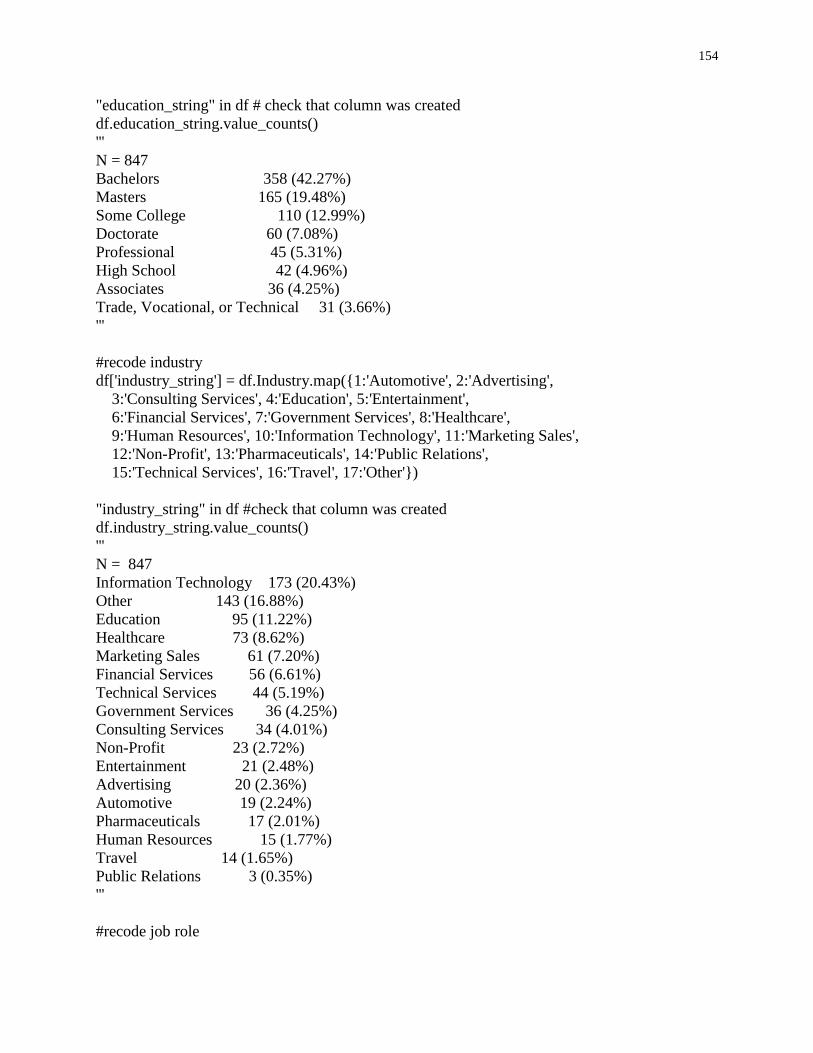
154

"education_string" in df # check that column was created

df.education_string.value_counts()

'''

N = 847

Bachelors 358 (42.27%)

Masters 165 (19.48%)

Some College 110 (12.99%)

Doctorate 60 (7.08%)

Professional 45 (5.31%)

High School 42 (4.96%)

Associates 36 (4.25%)

Trade, Vocational, or Technical 31 (3.66%)

'''

#recode industry

df['industry_string'] = df.Industry.map({1:'Automotive', 2:'Advertising',

3:'Consulting Services', 4:'Education', 5:'Entertainment',

6:'Financial Services', 7:'Government Services', 8:'Healthcare',

9:'Human Resources', 10:'Information Technology', 11:'Marketing Sales',

12:'Non-Profit', 13:'Pharmaceuticals', 14:'Public Relations',

15:'Technical Services', 16:'Travel', 17:'Other'})

"industry_string" in df #check that column was created

df.industry_string.value_counts()

'''

N = 847

Information Technology 173 (20.43%)

Other 143 (16.88%)

Education 95 (11.22%)

Healthcare 73 (8.62%)

Marketing Sales 61 (7.20%)

Financial Services 56 (6.61%)

Technical Services 44 (5.19%)

Government Services 36 (4.25%)

Consulting Services 34 (4.01%)

Non-Profit 23 (2.72%)

Entertainment 21 (2.48%)

Advertising 20 (2.36%)

Automotive 19 (2.24%)

Pharmaceuticals 17 (2.01%)

Human Resources 15 (1.77%)

Travel 14 (1.65%)

Public Relations 3 (0.35%)

'''

#recode job role

155

df['job_level_string'] = df.Job_Level.map({1:'Intern', 2:'Entry Level',

3:'Analyst / Associate', 4:'Project or Product Manager', 5:'Manager',

6:'Senior Manager', 7:'Director', 8:'Director', 9:'Senior Director',

10:'Vice President', 11:'Senior Vice President', 12:'C Level Executive',

13:'President / CEO', 14:'Owner'})

"job_level_string" in df #check that column was created

df.job_level_string.value_counts()

'''

N = 847

Analyst / Associate 250 (29.52%)

Entry Level 201 (23.73%)

Manager 140 (16.53%)

Project or Product Manager 105 (12.40%)

Senior Manager 39 (4.60%)

Intern 36 (4.25%)

Owner 33 (3.90%)

Director 30 (3.54)

President / CEO 4 (0.47%)

Senior Director 4 (0.47%)

C Level Executive 2 (0.24%)

Vice President 2 (0.24%)

Senior Vice President 1 (0.12%)

'''

#descriptives for average hours worked

df.Hours_Week.describe() #returns a values_counts() type result, these should be float numbers

type(df.Hours_Week) #check the data type for this column, it's a series object

df['hours'] = pd.to_numeric(df.Hours_Week, errors='coerce')

#convert the object to a float, by creating a new column

#drop the other column

df.drop(['Hours_Week'], axis =1, inplace=True)

#run descriptives on hours

df.hours.describe()

df.hours.median()

df.hours.mode()

'''

count 900.000000

mean 45.213611

std 100.274964

min 0.000000

25% 40.000000

156

50% 40.000000

75% 45.000000

max 3000.000000

We can see that there are some values that are not within an expected range

given that participants had been working full time (min of 32 hours), and there

are not 3,000 hours in a week, so we replace out of range values with the

mode/median.

Total cases = 54

'''

df.hours.replace(0, 40, inplace=True)

#since there are multiple let's switch how we use replace

df.replace({'hours': {0:40, 1:40, 2:40, 3:40, 4:40, 5:40, 6:40, 7:40, 8:40, 9:40,

10:40, 15:40, 16:40, 20:40, 24:40, 25:40, 26:40, 28:40,

30:40, 3000:40, 480:40, 150:40}}, inplace=True)

#re-run describe to verify that the descriptives look right

df.hours.describe()

'''

count 846.000000

mean 42.662825

std 7.659092

min 32.000000

25% 40.000000

50% 40.000000

75% 45.000000

max 100.000000

'''

#recode salary

df['salary_string'] = df.Salary.map({1:'10-20K', 2:'21-40K', 3:'41-60K',

4:'61-80K', 5:'81-100K', 6:'101-149K', 7:'150K+'})

"salary_string" in df #check that column was created

df.salary_string.value_counts()

'''

N = 847

10-20K 283 (33.42%)

21-40K 273 (32.23%)

41-60K 148 (17.47%)

61-80K 69 (8.15%)

81-100K 36 (4.25%)

101-149K 22 (2.60%)

157

150K+ 16 (1.89%)

'''

#recode age

df['age_string'] = df.Age.map({1:'18-24', 2:'25-34', 3:'35-44', 4:'45-55',

5:'55-64', 6:'65+'})

"age_string" in df

df.age_string.value_counts()

'''

N = 847

25-34 466 (55.02%)

18-24 232 (27.39%)

35-44 103 (12.16%)

45-55 34 (4.01%)

55-64 11 (1.30%)

65+ 1 (0.12%)

'''

'''We need to recode all of our Job Performance variables from their current

Likert 1-5 scale to a 0-4 scale, so we can properly create our job performance

variable and run diagnostics on items. To do this, we do vector addition (or

really subtraction) because we are subtracting 1 from every column.

We can either create a list of the columns and then write a for loop or do a

more elegant vector addition

'''

#changing using a loop, create a list of column headers then loop through and

#subtract 1

jp = ['Job_Performance1',

'Job_Performance2',

'Job_Performance3',

'Job_Performance4',

'Job_Performance5',

'Job_Performance6',

'Job_Performance7',

'Job_Performance8',

'Job_Performance9',

'Job_Performance10',

'Job_Performance11',

'Job_Performance12',

'Job_Performance13',

'Job_Performance14',

'Job_Performance15',

158

'Job_Performance16',

'Job_Performance17',

'Job_Performance18']

#subtract 1 using a for loop

#for col in jp:

# df[col] = df[col] -1

#vector addition

df[jp] = df[jp] -1

#verify that the range is now 0-4

df.Job_Performance1.describe()

'''

count 847.000000

mean 2.870130

std 1.047181

min 0.000000

25% 2.000000

50% 3.000000

75% 4.000000

max 4.000000

Name: Job_Performance1, dtype: float64

'''

df.Job_Performance18.describe()

'''

count 847.000000

mean 1.343566

std 1.208237

min 0.000000

25% 0.000000

50% 1.000000

75% 2.000000

max 4.000000

Name: Job_Performance18, dtype: float64

'''

'''

CREATE JOB PERFORMANCE VARIABLES OF TASK PERFROAMCNE, CONTEXTUAL

PERFORMANCE,

AND COUNTER PRODUCTIVE PERFORMANCE

'''

#create variables for TASK PERFORMANCE and look at descriptives for this variable

df['task_performance'] = ((df.Job_Performance1 + df.Job_Performance2 + df.Job_Performance3

+

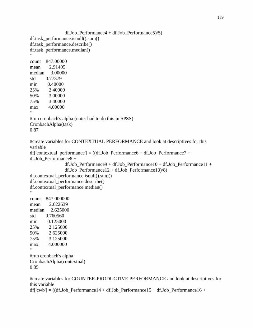
159

df.Job_Performance4 + df.Job_Performance5)/5)

df.task_performance.isnull().sum()

df.task_performance.describe()

df.task_performance.median()

'''

count 847.00000

mean 2.91405

median 3.00000

std 0.77379

min 0.40000

25% 2.40000

50% 3.00000

75% 3.40000

max 4.00000

'''

#run cronbach's alpha (note: had to do this in SPSS)

CronbachAlpha(task)

0.87

#create variables for CONTEXTUAL PERFORMANCE and look at descriptives for this

variable

df['contextual_performance'] = ((df.Job_Performance6 + df.Job_Performance7 +

df.Job_Performance8 +

df.Job_Performance9 + df.Job_Performance10 + df.Job_Performance11 +

df.Job_Performance12 + df.Job_Performance13)/8)

df.contextual_performance.isnull().sum()

df.contextual_performance.describe()

df.contextual_performance.median()

'''

count 847.000000

mean 2.622639

median 2.625000

std 0.760560

min 0.125000

25% 2.125000

50% 2.625000

75% 3.125000

max 4.000000

'''

#run cronbach's alpha

CronbachAlpha(contextual)

0.85

#create variables for COUNTER-PRODUCTIVE PERFORMANCE and look at descriptives for

this variable

df['cwb'] = ((df.Job_Performance14 + df.Job_Performance15 + df.Job_Performance16 +

160

df.Job_Performance17 + df.Job_Performance18)/5)

df.cwb.isnull().sum()

df.cwb.describe()

df.cwb.median()

'''

count 847.000000

mean 1.246753

std 0.949349

min 0.000000

25% 0.600000

50% 1.000000

75% 1.800000

max 4.000000

'''

#run cronbahc's alpha:

CronbachAlpha(cwb)

0.87

'''

CREATE IMPRESSION MANAGEMENT VARIABLE

note: initially I created mean scaled scores, but the original manuscript detailing the creation of

this measure states that scores should be summed. I've checked both variable creation approaches

and

they do not change the relationship with LIWC pronoun categories, it only changes the values of

the

descriptive statistics reported

'''

#df['impression'] = ((df.Impression_Work1 + df.Impression_Work2 + df.Impression_Work3 +

# df.Impression_Work4 + df.Impression_Work5 + df.Impression_Work6 +

# df.Impression_Work7 + df.Impression_Work8 + df.Impression_Work9 +

# df.Impression_Work10)/10)

#

#df.impression.isnull().sum()

#df.impression.describe()

#df.impression.median()

'''

impression management, full variable

count 847.000000

mean 4.292798

median 4.300000

std 1.082532

min 1.000000

25% 3.700000

50% 4.300000

75% 5.000000

max 7.000000

161

'''

#run cronbahc's alpha

CronbachAlpha(impression)

0.84

df['impression_other'] = (df.Impression_Work1 + df.Impression_Work2 + df.Impression_Work3

+

df.Impression_Work4 + df.Impression_Work5)

df.impression_other.describe()

df.impression_other.median()

'''

count 847.000000

mean 16.345927

median 16.000000

std 7.596475

min 5.000000

25% 10.000000

50% 16.000000

75% 22.000000

max 35.000000

'''

#run cronbahc's alpha

CronbachAlpha(impression_other)

0.87

df['impression_self'] = (df.Impression_Work6 + df.Impression_Work7 + df.Impression_Work8 +

df.Impression_Work9 + df.Impression_Work10)

df.impression_self.describe()

df.impression_self.median()

'''

count 847.000000

mean 26.603306

median 28.000000

std 6.114038

min 5.000000

25% 23.000000

50% 28.000000

75% 31.000000

max 35.000000

'''

#run cronbahc's alpha

CronbachAlpha(impression_self)

0.84

'''

162

CREATE SPOT-THE-WORD TEST SCORE

'''

df['stw_score'] = df[["Spot_The_Word_Test:chariot", "Spot_The_Word_Test:lentil",

"Spot_The_Word_Test:stamen", "Spot_The_Word_Test:comet",

"Spot_The_Word_Test:pylon", "Spot_The_Word_Test:flannel",

"Spot_The_Word_Test:fender", "Spot_The_Word_Test:joust",

"Spot_The_Word_Test:mantis", "Spot_The_Word_Test:sterile",

"Spot_The_Word_Test:monotheism", "Spot_The_Word_Test:stallion",

"Spot_The_Word_Test:rictus", "Spot_The_Word_Test:byzantine",

"Spot_The_Word_Test:monologue", "Spot_The_Word_Test:elegy",

"Spot_The_Word_Test:malign", "Spot_The_Word_Test:gelding",

"Spot_The_Word_Test:bulliner", "Spot_The_Word_Test:visage",

"Spot_The_Word_Test:oratory", "Spot_The_Word_Test:meridian",

"Spot_The_Word_Test:strumpet", "Spot_The_Word_Test:equine",

"Spot_The_Word_Test:riposte", "Spot_The_Word_Test:valance",

"Spot_The_Word_Test:introvert", "Spot_The_Word_Test:penumbra",

"Spot_The_Word_Test:malinger", "Spot_The_Word_Test:gammon",

"Spot_The_Word_Test:coracle", "Spot_The_Word_Test:paramour",

"Spot_The_Word_Test:octaroon", "Spot_The_Word_Test:carnation",

"Spot_The_Word_Test:agnostic", "Spot_The_Word_Test:plinth",

"Spot_The_Word_Test:thole", "Spot_The_Word_Test:reform",

"Spot_The_Word_Test:wraith", "Spot_The_Word_Test:pristine",

"Spot_The_Word_Test:pauper", "Spot_The_Word_Test:baleen",

"Spot_The_Word_Test:palindrome", "Spot_The_Word_Test:hedgehog",

"Spot_The_Word_Test:ferret", "Spot_The_Word_Test:drumlin",

"Spot_The_Word_Test:texture", "Spot_The_Word_Test:isomorphic",

"Spot_The_Word_Test:vitriol", "Spot_The_Word_Test:farrago",

"Spot_The_Word_Test:hermeneutic", "Spot_The_Word_Test:chaos",

"Spot_The_Word_Test:devastate", "Spot_The_Word_Test:peremptory",

"Spot_The_Word_Test:camera", "Spot_The_Word_Test:roster",

"Spot_The_Word_Test:accolade", "Spot_The_Word_Test:pleonasm",

"Spot_The_Word_Test:infiltrate",

"Spot_The_Word_Test:mystical"]].sum(axis=1)

df.stw_score.isnull().sum()

df.stw_score.describe()

df.stw_score.median()

'''

count 847.000000

mean 45.518300

median 49.000000

std 12.008836

min 0.000000

25% 44.000000

50% 49.000000

75% 52.000000

max 59.000000

163

alpha 0.951000

'''

#run cronbahc's alpha

0.87

'''

CREATE DUMMY VARIABLES

'''

#AGE

age_dummy = pd.get_dummies(df['age_string'], prefix='age') #create dummy variable dataframe

df1 = pd.concat([df, age_dummy], axis=1) #join dummy dataframe to original dataframe

df1.drop(['age_25-34'], inplace=True, axis=1)

#drop one of the dummy variables since it is redundent (k-1)

#here we drop the largest group, which is 25-34 year olds to make that our reference group

#SEX: already created since it is dichotomous and we recoded to 0 and 1 earlier

#RACE

race_dummy = pd.get_dummies(df1['race_string'], prefix='race') #create dummy variable

dataframe

df2 = pd.concat([df1, race_dummy], axis=1) #join dummy dataframe to original dataframe

df2.drop(['race_White'], inplace=True, axis=1)

#drop one of the dummy variables since it is redundent (k-1)

#here we drop race_white dummary variable, making whites our reference group

#INDUSTRY

industry_dummy = pd.get_dummies(df1['industry_string'], prefix='industry')

#create dummy variable dataframe

df3 = pd.concat([df2, industry_dummy], axis=1) #join dummy dataframe to original dataframe

df3.drop(['industry_Information Technology'], inplace=True, axis=1)

#drop one of the dummy variables since it is redundent (k-1)

#here we drop Information Technology dummary variable, making Information Technology our

reference group

#SALARY

salary_dummy = pd.get_dummies(df1['salary_string'], prefix='salary')

#create dummy variable dataframe

df4 = pd.concat([df3, salary_dummy], axis=1) #join dummy dataframe to original dataframe

df4.drop(['salary_21-40K'], inplace=True, axis=1)

#drop one of the dummy variables since it is redundent (k-1)

#here we drop salary_21-40K dummary variable, making 21-40K our reference group

#JOB ROLE

job_level_dummy = pd.get_dummies(df1['job_level_string'], prefix='job_level')

#create dummy variable dataframe

df5 = pd.concat([df4, job_level_dummy], axis=1) #join dummy dataframe to original dataframe

164

df5.drop(['job_level_Analyst / Associate'], inplace=True, axis=1)

#drop one of the dummy variables since it is redundent (k-1)

#here we drop salary_21-40K dummary variable, making 21-40K our reference group

#rename df5 to final

final = df5

'''

Read in both the final survey data and the text analylsis file generated by LIWC

'''

#cleaned up survey data, with dummy variables

df = pd.read_csv('dissertation_complete_847n_dummies.csv"', header=0, encoding='utf-8')

#text analytics file generated by liwc

dft =

pd.read_csv('C:\Users\joshuaw\Documents\PhD_Year_5\Data\liwc_results_all_resumes_1030_fi

les.csv',

header=0, encoding='utf-8')

#join the two files on the "Response_ID", we do an inner join because we only want cases that

are in

#both the survey data and liwc data sets.

df = pd.merge(df, dft, how='inner', left_on='Response_ID', right_on='Response_ID')

#write the final, analysis ready file to a csv

df.to_csv("dissertation_complete_847n_dummies.csv", sep=',', encoding='utf-8', index=False,

header=True)

165

Appendix G

Various Functions of First-Person Plural Pronouns (e.g. “We”), Adapted from Pennebaker, 2011

The word “we” has at least five different functions.

You-and-I We

This is the inclusive “we.” It is an identification that a specific person and I are part of the

same group. In other words, it indicates a shared identity. However, this can be slightly

problematic. For example, I might think that you and I are in the same group, but you might not.

My-Friends-and-Not-You We

This form of we often occurs when talking with people about an event or experience that

you shared but not with the people with whom you are speaking. For example, you might be

relating a story to your coworker about how you and your grad school mates checked out a new

whiskey bar in town. The “we” in that conversation is exclusionary; it refers to a different group,

which does not include your coworker.

We-as-You We

This usage of “we” is actually cordially asking or telling someone else to do something.

For example, during a meeting, I might say, “Can we please stop using buzz words like ‘machine

learning’ and ‘big data’ without first establishing a common understanding of these words?”

My-Friends-and-Not-You We and We-as-You We and Power

The two prior functions of “we” are used more often by those higher in social status and

power. For example, your boss’s boss is more likely to use these forms of “we” than your direct

report. Your boss’s boss is also more likely to talk more loudly than you, interrupt you, stand or

sit close to you, and take up more physical space than you.

166

We-as-I We

This is the royal “we.” It is used to diffuse responsibility and imply support from others

who may or may not exist. For example, a reviewer might say, “We felt the theory you presented

was absurdly outrageous. You might as well have theorized that unicorns and time travel are

possible.” The only person of this opinion was the particular reviewer. (Note: this example

sentence was inspired by true events but does not reflect the exact phrasing by any reviewer).