1

Predicting Distress in European Banks1

Frank Betz European Investment Bank

Silviu Oprică European Central Bank

Tuomas A. Peltonen European Central Bank

Peter Sarlin2 Åbo Akademi University

This version: January 29, 2013 First draft: May 16, 2012

Abstract The paper develops an early-warning model for predicting vulnerabilities leading to distress in European banks using both bank and country-level data. As outright bank failures have been rare in Europe, we introduce a novel dataset that complements bankruptcies and defaults with state interventions and mergers in distress. The signals of the early-warning model are calibrated not only according to the policymaker’s preferences between type I and II errors, but also to take into account the potential systemic relevance of each individual financial institution. The key findings of the paper are that complementing bank-specific vulnerabilities with indicators for macro-financial imbalances improves model performance and yields useful out-of-sample predictions of bank distress during the current financial crisis. JEL Codes: E44, E58, F01, F37, G01. Keywords: Bank distress; early-warning model; prudential policy; signal evaluation 1 The authors want to thank Riina Vesanen for excellent research assistance and colleagues at the ECB, particularly Carsten Detken, Jean-Paul Genot, Marco Gross, Urszula Kochanska, Markus Kolb, Bernd Schwaab, Kostas Tsatsaronis and Joseph Vendrell, both for discussions and sharing data. Thanks also to participants at the ECB Financial Stability seminar on 16 May 2012 and the ECB Financial Stability conference: Methodological advances and policy issues on 14–15 June 2012 in Frankfurt am Main, Germany, particularly to Dilruba Karim, the third MAFIN conference on 19–21 September 2012 in Genoa, Italy, CEQURA Conference on Advances in Financial and Insurance Risk Management on 24–26 September 2012 in Munich, Germany, and the second conference of the ESCB Macro-prudential Research Network on 30–31 October 2012 in Frankfurt am Main, Germany, particularly to Philip Davis. All remaining errors are our own. Peter Sarlin gratefully acknowledges the financial support of the Academy of Finland (grant no. 127592). The views presented in the paper are those of the authors only and do not necessarily represent the views of the European Central Bank, the Eurosystem or the European Investment Bank. 2 Corresponding author: Peter Sarlin, Department of Information Technologies, Åbo Akademi University, Turku Centre for Computer Science, Joukahaisenkatu 3–5, 20520 Turku, Finland. Email: psarlin@abo.fi tel. +358 2 215 4670.

2

Non-technical summary The global financial crisis has brought a large number of European banks to the brink of collapse. Moreover, beyond the direct bailout costs and output losses, the interplay of fiscally strained sovereigns and weak banking systems that characterize the ongoing sovereign debt crisis in Europe show the important role of the euro area banking sector for the stability of the entire European Monetary Union. Thus, the motivation for an early-warning model for European banks is obvious. To derive an early-warning model for European banks, this paper introduces a novel dataset of bank distress events. As bank defaults are rare in Europe, the data set complements bankruptcies, liquidations and defaults by also taking into account state interventions, and mergers in distress. State interventions comprise capital injections and asset reliefs (asset protection and guarantees). A distressed merger occurs if i) a parent receives state aid within 12 months after the merger or ii) if a merged entity has a coverage ratio smaller than 0 within 12 months before the merger. The outbreak of a financial crisis is known to be difficult to predict (e.g., Rose and Spiegel, 2011). Recently, the early-warning model literature has therefore focused on detecting underlying vulnerabilities, and finding common patterns preceding financial crises (e.g., Reinhart and Rogoff, 2008; 2009). Thus, this paper focuses on predicting vulnerable states, where one or multiple triggers could lead to a bank distress event. The early-warning model applies a micro-macro perspective to measure bank vulnerability. Beyond bank-specific and banking-sector vulnerability indicators, the paper uses measures of macroeconomic and financial imbalances from the EU Alert Mechanism Report related to the EU Macroeconomic Imbalance Procedure (MIP). The models derive bank-specific probabilities of being in a vulnerable state, but a policy maker has to know when to act. The paper uses the state-of-the-art methodology developed in Sarlin (2012) to evaluate the signals of the model. The approach takes into account the policymaker's preferences between type I and type II errors, the uneven frequency of tranquil and distress events, and the systemic relevance of the bank. This paper presents the first application of the evaluation framework to a bank-level model and represent a bank's systemic relevance with its size. Thus, the early-warning model is better suited to predict systemic banking crises and to analyse systemic risks. Regarding the main findings of the paper, the estimation results provide useful insights into determinants of banking sector fragility in Europe. We find that complementing bank-specific vulnerabilities with indicators of macro-financial imbalances improves model performance. Thus, the results of the paper also confirm the usefulness of the vulnerability indicators introduced recently with respect to the

3

EU Macroeconomic Imbalance Procedure (MIP). Instead, indicators of imbalances in countries' banking-sectors only marginally improve model performance. Moreover, the paper shows that an early-warning exercise with the model shows that using only publicly available data yields useful out-of-sample predictions of bank distress during the current financial crisis (2007Q1-2011Q4). Finally, the results of the evaluation framework show that a policymaker has to be substantially more concerned of missing bank distress than issuing false alarms for the model to be useful. This is intuitive if we consider that an early-warning signal triggers an in-depth review of fundamentals, business model and peers of the bank predicted to be in distress. Should the analysis reveal that the signal is false, there is no loss of credibility on behalf of the policy authority. The evaluations also imply that it is important to give more emphasis to systemically important and large banks for a policymaker concerned with systemic risk.

4

1. Introduction

The global financial crisis has brought a large number of European banks to the brink of collapse. Data from the European Commission show that the amount of aid granted by EU states to stabilise the EU banking sector that had been used by the end of 2010 had exceeded €1.6 trillion, more than 13% of EU GDP. Though large, the immediate bailout costs account only for a moderate share of the total cost of a systemic banking crisis. As shown in Dell Arriccia et al. (2010) and Laeven and Valencia (2008, 2010, 2011) among others, the output losses of previous banking crises have averaged around 20-25% of GDP. In addition, the interplay of fiscally strained sovereigns and weak banking systems that characterize the ongoing sovereign debt crisis show the crucial role of the euro area banking sector for the stability of the entire European Monetary Union. The rationale behind an early-warning model for European banks is thus clear. To derive an early-warning model for European banks, this paper introduces a novel dataset of bank distress events. As bank defaults are rare in Europe, the dataset complements bankruptcies, liquidations and defaults by also taking into account state interventions, and mergers in distress. State interventions comprise capital injections and asset reliefs (asset protection and guarantees). A distressed merger occurs if i) a parent receives state aid within 12 months after the merger or ii) if a merged entity has a coverage ratio smaller than 0 within 12 months before the merger. The outbreak of a financial crisis is notoriously difficult to predict (e.g., Rose and Spiegel, 2011). Recently, the early-warning model literature has therefore focused on detecting underlying vulnerabilities, and finding common patterns preceding financial crises (e.g., Reinhart and Rogoff, 2008; 2009). Thus, this paper focuses on predicting vulnerable states, where one or multiple triggers could lead to a bank distress event. The early-warning model applies a micro-macro perspective to measure bank vulnerability. Beyond bank-specific and banking-sector vulnerability indicators, the paper uses measures of macroeconomic and financial imbalances from the EU Alert Mechanism Report related to the EU Macroeconomic Imbalance Procedure (MIP). The models derive bank-specific probabilities of being in a vulnerable state, but a policy maker has to know when to act. The paper uses the state-of-the-art methodology developed in Sarlin (2012) to evaluate the signals of the model. The approach takes into account the policymaker's preferences between type I and type II errors, the uneven frequency of tranquil and distress events, and the systemic relevance of the bank. This paper presents the first application of the evaluation framework to a bank-level model and represent a bank's systemic relevance with its size. Thus, the early-warning model is better suited to predict systemic banking crises and to analyse systemic risks.

5

The results provide useful insights into determinants of banking sector fragility in Europe. We find that complementing bank-specific vulnerabilities with indicators of macro-financial imbalances improves model performance. Thus, the results of the paper also confirm the usefulness of the vulnerability indicators introduced recently with respect to the EU Macroeconomic Imbalance Procedure (MIP). Instead, indicators of imbalances in countries' banking-sectors only marginally improve model performance. Moreover, the paper shows that an early-warning exercise with the model shows that using only publicly available data yields useful out-of-sample predictions of bank distress during the current financial crisis (2007Q1-2011Q4). Finally, the results of the evaluation framework show that a policymaker has to be substantially more concerned of missing bank distress than issuing false alarms for the model to be useful. This is intuitive if we consider that an early-warning signal triggers an in-depth review of fundamentals, business model and peers of the bank predicted to be in distress. Should the analysis reveal that the signal is false, there is no loss of credibility on behalf of the policy authority. The evaluations also imply that it is important to give more emphasis to systemically important and large banks for a policymaker concerned with systemic risk. The paper is organized as follows. Section 2 provides a brief review of the related literature. Section 3 describes the data used to define bank distress events as well as the construction of the vulnerability indicators. Section 4 describes the methodological aspects of the early-warning model. Section 5 presents results on determinants of distress and predictive performance, and Section 6 discusses their robustness. Finally, Section 7 concludes the paper. Technical aspects, such as variable definitions, data sources and further robustness tests, are found in the Appendix.

2. Related literature

The present paper is linked to two strands of literature. First, it relates to papers predicting failures or distress at the bank level, and second, to studies on optimal early warning signals for policymakers. The literature on individual bank failures draws heavily on the Uniform Financial Rating System, informally known as the CAMEL ratings system, introduced by U.S. regulators in 1979, where the letters refer to Capital adequacy, Asset quality, Management quality, Earnings, Liquidity. Since 1996 the rating system includes also Sensitivity to Market Risk (i.e., CAMELS). The CAMELS rating system is an internal supervisory tool for evaluating the soundness of financial institutions on a uniform basis and for identifying those institutions requiring special supervisory attention or concern. Several studies find that banks' balance-sheet indicators measuring capital adequacy, asset quality, and liquidity are significant in predicting bank failures in

6

accounting-based models (e.g., Thomson (1992) and Cole and Gunther (1995, 1998)). Other studies augment the pure accounting-based models with macroeconomic indicators and asset prices. Several papers, mainly based on US bank data, suggest that both macroeconomic and market price-based indicators contain useful predictive information not contained in the CAMELS indicators (e.g., Flannery (1998), González-Hermosillo (1999), Jagtiani and Lemieux (2001), Curry et al. (2007), Bharath and Shumway (2008), or Campbell et al. (2008)). There is not, however a consensus on the findings in the US, which hinders a direct comparison to the findings on European banks in this study. Most papers analyzing individual bank failures or distress events focus on U.S. banks or a panel of banks across countries, while there are only a few studies dealing with European banks. Data limitations set by the lack of direct failures in core Europe is illustrated by some recent works: Männasoo and Mayes (2009) focus on Eastern European banks, Ötker and Podpiera (2010) create distress events from Credit Default Swaps (CDS), and Poghosyan and Cihák (2011) create events by keyword searches in news articles. These suffer, however, from three respective limitations: no focus on the entire Europe, in particular the core, the use of CDS limits the sample to listed banks, and data from news articles are inherently noisy. The literature on country-level banking crises is also broad and has most often focused on continents, if not pursuing a fully global approach. Demirgüç-Kunt and Detragiache (2000), Davis and Karim (2008a,b) and Sun (2011) analyse banking crises with a global country coverage, whereas Hutchison (2003) and Mody and Sandri (2012) focus on European countries, where the latter study focuses on the recent crisis. Regarding studies optimal early warning signals for a policymaker, a seminal paper by Kaminsky et al. (1998) introduces the so-called “signal” approach to evaluate the early-warning properties of univariate indicator signals when they exceeds a predefined threshold. The threshold is set to minimize the noise-to-signal ratio, given by the number of false alarms relative to the correct calls. Many later studies, such as Berg and Pattillo (1999a) and Edison (2003), while introducing a discrete-choice model, do not adopt a structured approach to evaluate model performance. An issue addressed by Demirgüç-Kunt and Detragiache (2000) is the introduction of a loss function of a policymaker that considers costs for preventive actions and relative preferences between missing crises (type I errors) and false alarms (type II errors). The authors show that optimising model thresholds on the basis of the noise-to-signal ratio can lead to sub-optimal results under some preference schemes.3 Alessi and Detken (2011) apply the loss function approach to asset price boom/bust cycles and extend it by also introducing a measure that accounts for the usefulness of

3 If banking crises are rare events and the cost of missing a crisis is high relative to that of issuing a false alarm, minimising the noise-to-signal ratio could lead to many missed crises. As a consequence, the selected threshold could be sub-optimal from the point of view of the preferences of policymakers.

7

disregarding the signals of a model. Sarlin (2012) further extends the literature by amending the policymaker’s loss function and usefulness measure in the framework by Alessi and Detken (2011) to include unconditional probabilities of the events, as was previously done in Demirgüç-Kunt and Detragiache (2000), and computes a measure called relative Usefulness. By computing the share of available Usefulness that a model captures, the relative Usefulness facilitates interpretation of the measure. Furthermore, the signal evaluation scheme also accounts for the systemic relevance of each individual entity, e.g., bank or country, as well as further augments the usefulness measure by focusing on the share of available usefulness that the model captures.

3. Data

We construct the sample based on availability of balance-sheet and income-statement data in Bloomberg. The observation period starts in Q1 2000 and ends in Q4 2011. We obtain data on 546 banks with a minimum of EUR 1bn in total assets during the period under consideration (in total 26,852 observations). By this rule, we focus on large banks with significance for system stability. The sample covers banks in all EU countries but Cyprus, Estonia, Lithuania and Romania. We do our best efforts to reconstruct the information set that would have been available to investors at each point of time. Thus, for instance, if a bank reports its accounts at annual frequency, we use this information in four subsequent quarters. The dataset consists of two parts: bank distress events and vulnerability indicators. We describe them in the following. 3.1. Identifying bank distress events Given that actual bank failures are rare in Europe, identification of bank distress events is challenging. Thus, in addition to bankruptcies, liquidations, and defaults, the paper also takes into account state interventions and forced mergers to represent bank distress. First, we use data on bankruptcies, liquidations and defaults to capture direct bank failures. A bankruptcy is defined to occur if the net worth of a bank falls below the country-specific guidelines, whereas liquidations occur if a bank is sold as per the guidelines of the liquidator in which case the shareholders may not receive full payment for their ownership. We define two types of defaults as follows: a default occurs i) if a bank has failed to pay interest or principal on at least one financial obligation beyond any grace period specified by the terms, or ii) if a bank completes a distressed exchange, in which at least one financial obligation is repurchased or replaced by other instruments with a diminished total value. The data on bankruptcies and liquidations are retrieved from Bankscope, while defaults are obtained from annual compendiums of corporate defaults by Moody’s and Fitch. We define a

8

distress event to start when the failure is announced and to end when the failure de facto occurs. This method leads to 13 distress events at the bank-quarter level, of which most are defaults. Second, we use data on state support to detect banks in distress. A bank is defined to be in distress if it receives a capital injection by the state or participates in asset relief programmes (asset protection or asset guarantees). This definition focuses on assistance on the asset side and does hence not include liquidity support or guarantees on banks’ liabilities. The state aid measures are based on data from the European Commission as well as data collected by the authors from market sources (Reuters and Bloomberg). Events in this category are defined to last from the announcement of the state support to the execution of the state support programme. This approach leads to 153 distress events, which shows the extent to which state intervention is more common than outright default. Third, mergers in distress capture private sector solutions to bank distress. The merged entities are defined to be in distress if i) a parent receives state aid within 12 months after the merger or ii) if a merged entity has a coverage ratio smaller than 0 within 12 months before the merger. The coverage ratio is commonly used in the literature to define distressed banks (e.g., González-Hermosillo, 1999). The rationale for applying the rule only on mergers is that we want to capture banks that are forced to merge due to distress. A bank may have a negative coverage ratio, but still survive without external support. Data on mergers are obtained from Bankscope, whereas the coverage ratio is defined as the ratio of capital equity and loan reserves minus non-performing loans to total assets and computed using data from Bloomberg. While these definitions should thoroughly cover distressed mergers, the only caveat is a possible mismatch in sample coverage of the two data sources. The events identified using these definitions of distressed mergers were, however, cross-checked using market sources (Reuters and Bloomberg). We define the two types of distressed mergers to start and end as follows: i) to start when the merger occurs and end when the parent receives state aid and ii) to start when the coverage ratio falls below 0 (within 12 months before the merger) and end when the merger occurs. Based on this approach we identify 35 mergers in distress. In total, we obtain 194 distress events at the bank-quarter level. This figure is smaller than the sum of events across categories as they are not mutually exclusive. As a bank that experiences two distress events within one year is likely to be in distress also in between those events, we modify the bank-specific time series accordingly. While being a question of interest, we do not distinguish between the different types of distress events in the sequel of this paper. The low frequency of direct failures and distressed mergers hinders robust estimations of determinants for all three categories.

9

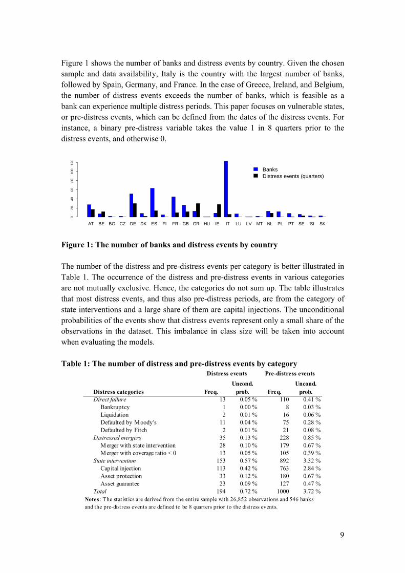
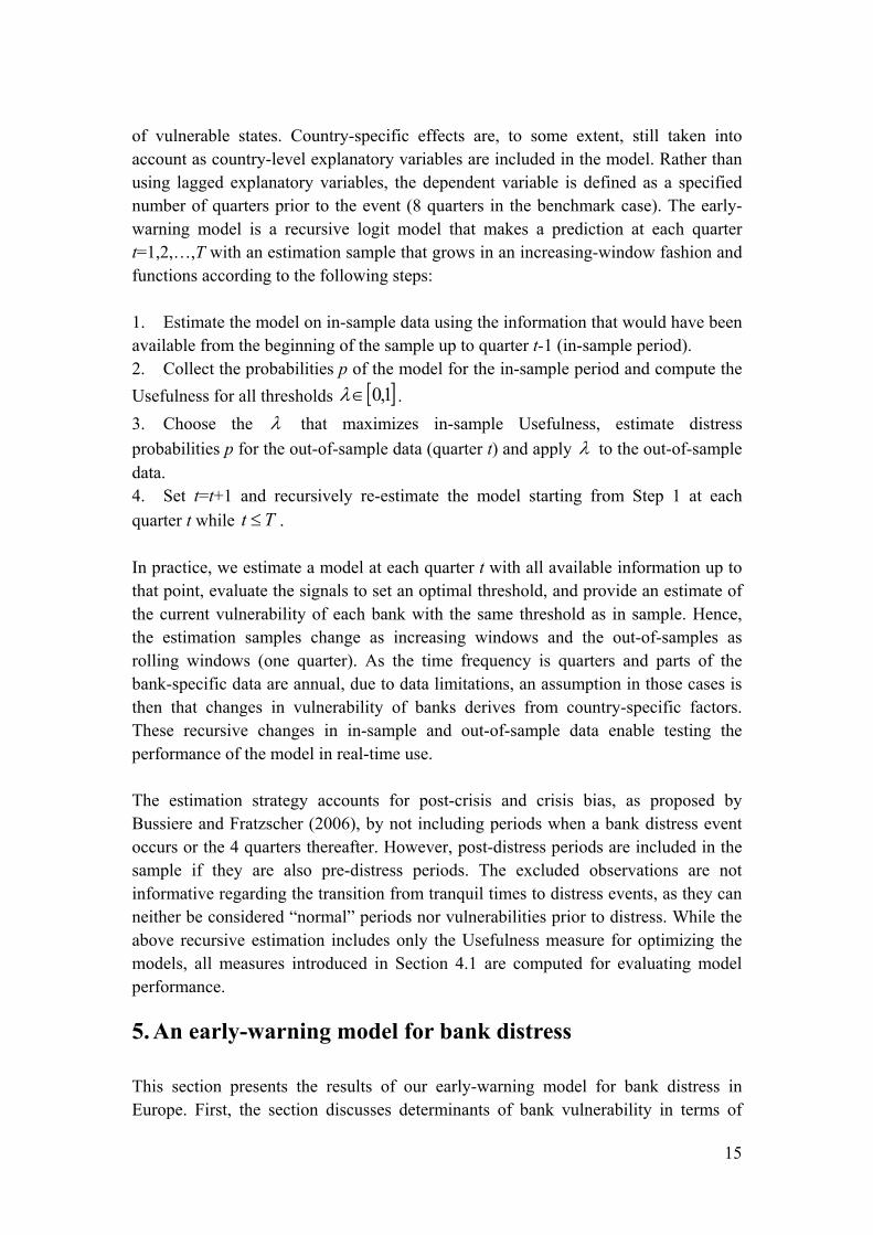
Figure 1 shows the number of banks and distress events by country. Given the chosen sample and data availability, Italy is the country with the largest number of banks, followed by Spain, Germany, and France. In the case of Greece, Ireland, and Belgium, the number of distress events exceeds the number of banks, which is feasible as a bank can experience multiple distress periods. This paper focuses on vulnerable states, or pre-distress events, which can be defined from the dates of the distress events. For instance, a binary pre-distress variable takes the value 1 in 8 quarters prior to the distress events, and otherwise 0.

AT BE BG CZ DE DK ES FI FR GB GR HU IE IT LU LV MT NL PL PT SE SI SK

02

04

06

08

01

00

12

0

BanksDistress events (quarters)

Figure 1: The number of banks and distress events by country The number of the distress and pre-distress events per category is better illustrated in Table 1. The occurrence of the distress and pre-distress events in various categories are not mutually exclusive. Hence, the categories do not sum up. The table illustrates that most distress events, and thus also pre-distress periods, are from the category of state interventions and a large share of them are capital injections. The unconditional probabilities of the events show that distress events represent only a small share of the observations in the dataset. This imbalance in class size will be taken into account when evaluating the models. Table 1: The number of distress and pre-distress events by category

Distress categories Freq.Uncond.

prob. Freq.Uncond.

prob.Direct failure 13 0.05 % 110 0.41 %

Bankruptcy 1 0.00 % 8 0.03 %Liquidation 2 0.01 % 16 0.06 %Defaulted by Moody's 11 0.04 % 75 0.28 %Defaulted by Fitch 2 0.01 % 21 0.08 %

Distressed mergers 35 0.13 % 228 0.85 %Merger with state intervention 28 0.10 % 179 0.67 %Merger with coverage ratio < 0 13 0.05 % 105 0.39 %

State intervention 153 0.57 % 892 3.32 %Capital injection 113 0.42 % 763 2.84 %Asset protection 33 0.12 % 180 0.67 %Asset guarantee 23 0.09 % 127 0.47 %

Total 194 0.72 % 1000 3.72 %

Distress events Pre-distress events

Notes: The statistics are derived from the entire sample with 26,852 observations and 546 banks and the pre-distress events are defined to be 8 quarters prior to the distress events.

10

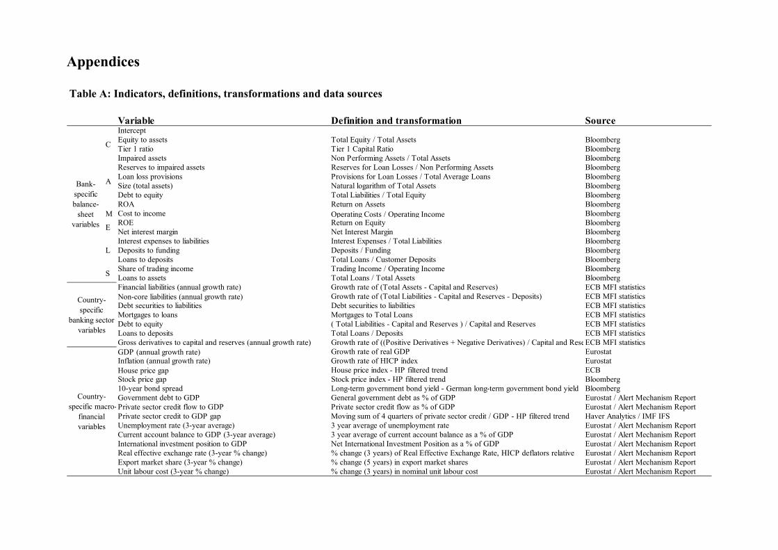
3.2. Vulnerability indicators The paper uses three categories of indicators in order to capture various aspects of a bank's vulnerability to distress. First, indicators from banks’ income statements and balance sheets measure bank-specific vulnerabilities. Following the literature, we use indicators to account for all dimensions in the CAMELS rating system (e.g., Flannery, 1998; González-Hermosillo, 1999; Poghosyan and Cihák, 2011). The indicators to proxy the CAMELS dimensions as follows. The equity-to-assets and Tier 1 capital ratio represent Capital adequacy (C) and are used to proxy the level of bank capitalization. Asset quality (A) is represented by return on assets, size of total assets, debt-to-equity ratio, impaired assets and loan loss provisions. The cost-to-income ratio represents Management quality (M), while return on equity (ROE) and net interest margin measure Earnings (E). Liquidity (L) is represented by the share of interest expenses to total liabilities, deposits-to-funding ratio and the ratio of loans to deposits. Finally, the share of trading income represents Sensitivity to market risk (S). We do not consider market-based indicators, such as proposed by Agarwal and Taffler (2008). The key reasons are two: i) we aim at predicting underlying vulnerabilities 1-3 years prior to distress, whereas market-based signals tend to have a shorter horizon, and ii) we aim at using a broad sample of banks, rather than only listed banks. Second, country-specific banking sector indicators represent imbalances at the level of banking systems. These indicators are often cited as key early-warning indicators for banking crises (e.g., Demirgüç-Kunt and Detragiache, 1998; 2000; Kaminsky and Reinhart, 1999). Moreover, there are currently efforts at the EU level to find a suitable vulnerability indicator for the banking/financial sector (EC, 2012). The indicators proxy the following types of imbalances: booms and rapid increases in banks’ balance sheets, e.g., growth in financial liabilities and non-core liabilities; securitization, e.g., debt securities to liabilities; property booms, e.g., mortgages-to-loans ratio; banking-system leverage, e.g., debt-to-equity and loans-to-deposits ratios; and banking-system exposures to derivatives contracts, e.g., gross derivatives to capital and reserves. The indicators used in the paper are described in Appendix A.1. All indicators except credit to GDP are constructed using the ECB’s statistics on the Balance Sheet Items (BSI) of the Monetary, Financial Institutions and Markets (MFI), whereas the credit-to-GDP indicator is calculated using data from Haver Analytics and the IMF International Financial Statistics database (IFS). Finally, country-specific macro-financial indicators identify macro-economic imbalances and control for conjunctural variation in asset prices and business cycles. To control for macro-economic imbalances, the paper uses the internal and external indicators from the EU Macroeconomic Imbalance Procedure (MIP), such as current account imbalances, unit labour costs, unemployment rate, and general government debt. Moreover, asset prices (stock and house price gaps) and business cycle indicators (real GDP growth and CPI inflation) capture conjunctural variation.

11

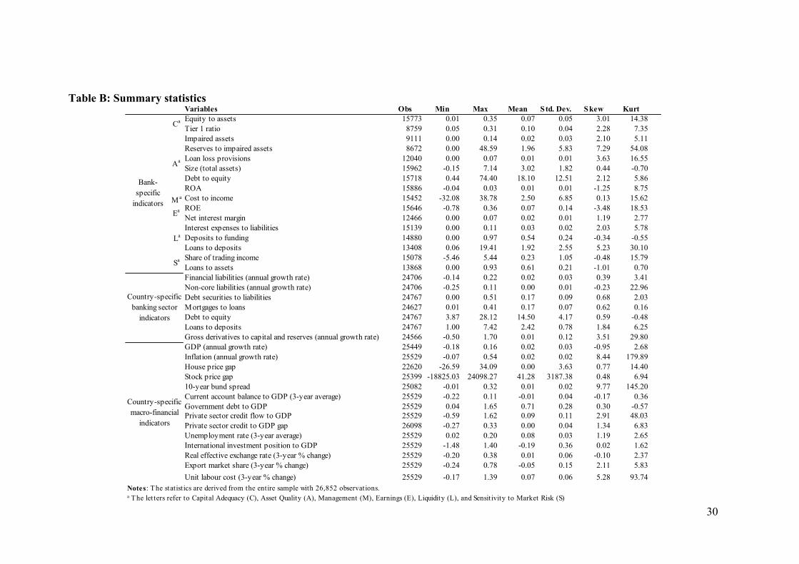
Appendix A.1 provides a more detailed description of the indicators. Most of the macro-financial indicators are retrieved from Eurostat and Bloomberg. Tables A and B in the Appendix describe the indicators used and their definitions and transformations, as well as their summary statistics. The statistical tests show that the data are non-normally distributed and exhibit most often a positive skew with a leptokurtic distribution. Table C in the Appendix shows the discriminatory power of the indicators through mean-comparison tests. The t-test results indicate that most variables are good candidates for discriminating between tranquil and vulnerable periods. Among bank-specific indicators, the cost-to-income ratio, share of trading income and loans to assets do not hold a promise to discriminate between the classes. Financial liabilities and gross derivatives are the poorest discriminators among banking-sector indicators, whereas inflation and stock-price gap are the poorest among macro-financial indicators.

4. Methodology

The methodology presented in this section consists of two building blocks: i) a framework for evaluating signals of early-warning models, and ii) the estimation and prediction methods. 4.1. Evaluation of model signals Early-warning models require evaluation criteria that account for the nature of the underlying problem. Distress events are oftentimes outliers in three aspects: the dynamics of the economy differ significantly from tranquil times, they are often costly, and they occur rarely. Given these properties, an evaluation framework that resembles the decision problem faced by a policymaker is of central importance. Designing a comprehensive evaluation framework for early-warning model signals is challenging as there are several political economy aspects to be taken into account. For instance, the frequency and optimal timing when the policymaker should signal a crisis might depend on potential inconsistencies between the maximisation of the policymaker’s own utility vs. social welfare. While important, these types of considerations are beyond the scope of this study. Thus, the signal evaluation framework focuses only on a policymaker with relative preferences between type I and II errors and the usefulness that she gets by using a model vs. not using it. As the focus is on detecting vulnerabilities and risks prior to distress, the ideal leading indicator can be represented by a binary state variable 1,0)( hC j for observation j

(where j=1,2,…,N) with a specified forecast horizon h. Let )(hC j be a binary

indicator that is one during pre-crisis periods and zero otherwise. For detecting events

jC using information from indicators, discrete-choice models can be used for

12

estimating probabilities of occurrence of crisis 1,0jp . To mimic the ideal leading

indicator, the probability p is transformed into a binary prediction Pj that is one if pj

exceeds a specified threshold 1,0 and zero otherwise. The correspondence

between the prediction Pj and the ideal leading indicator jC can be summarized into a

so-called contingency matrix. Actual class Cj

1 0

Predicted class Pj 1 True positive (TP) False positive (FP)

0 False negative (FN) True negative (TN)

While the elements of the matrix (frequencies of prediction-realization combinations) can be used for computing a wide range of measures4, a policymaker can be thought of mainly being concerned about two types of errors: giving false alarms and missing crises. The evaluation framework in this paper follows Sarlin (2012) for turning policymakers' preferences into a loss function, where the policymaker has relative preferences between type I and II errors. Type I errors represent the proportion of missed crises relative to the number of crises in the sample

( FNTPFNT /1,01 ), and type II errors the proportion of false alarms relative

to the number of tranquil periods in the sample ( TNFPFPT /1,02 ). Given

probabilities p of a model, the policymaker should choose a threshold such that her

loss is minimized. The loss of a policymaker consists of 1T and 2T , weighted

according to her relative preferences between missing crises and giving false

alarms 1 . By accounting for unconditional probabilities of crises 11 DPP

and tranquil periods 12 10 PDPP , the loss function is as follows:

2211 1 PTPTL , (1)

where 1,0 represents the relative preferences of missing events and 1 the

relative preferences of giving false alarms, 1T the type I errors and 1T the type II

errors. 1P refers to the size of the crisis class and 2P to the size of the tranquil class.

Using the loss function L , the Usefulness of a model can be defined in two ways.

First, the absolute Usefulness ( aU ) is given by:

4 Some of the commonly used simple evaluation measures are as follows. Recall positives (or TP rate) = TP/(TP+FN), Recall negatives (or TN rate) = TN/(TN+FP), Precision positives = TP/(TP+FP), Precision negatives = TN/(TN+FN), Accuracy = (TP+TN)/(TP+TN+FP+FN), FP rate = FP/(FP+TN), and FN rate = FN/(FN+TP).

13

)(1,min 21 LPPUa , (2)

which computes the extent to which a model performs better than no model at all. As the unconditional probabilities are commonly unbalanced and the policymaker may be more concerned about one class, a policymaker could achieve a loss of

1,min 21 PP by either always or never signalling an event. It is thus worth

noting that already an attempt to build an early-warning model for events with unbalanced events implicitly assumes a policymaker to be more concerned about the rare class. With a non-perfectly performing model, it would otherwise easily pay-off for the policymaker to always signal the high-frequency class.

Second, relative Usefulness rU is computed as follows:

,1,min 21

PP

UU a

r (3)

where the absolute Usefulness aU of the model is compared with the maximum

possible usefulness of the model, i.e., the loss of disregarding the model. That is, rU

reports aU as a percentage of the usefulness that a policymaker would gain with a

perfectly performing model. A policymaker may further want to enhance the representation of preferences by accounting for observation-specific differences in costs. In bank early-warning models, the bank-specific misclassification costs are highly related to the systemic or contagious relevance of an entity for the policymaker. While this relevance can be measured with network measures such as centrality, a simplified measure of relevance for the system in general is the size of the entity relative to the system's size (e.g., assets of a financial institution). Let jw be a bank-specific weight that approximates

the importance of correctly classifying observation j. Also, let jTP , jFP , jFN and

jTN be binary vectors of combinations of predictions and realizations rather than

only their sums. By multiplying each binary element of the contingency matrix by

jw , we can derive a policymaker's loss function with bank and class-specific

misclassification costs. Let 1T and 2T be weighted by jw to have weighted type I and

II errors:

N

j jjN

j jjN

j jjw FNwTPwFNwT1111 /1,0

N

j jjN

j jjN

j jjw TNwFPwFPwT1112 /1,0 .

14

As 1wT and 2wT are ratios of weights rather than ratios of binary values, the errors

1wT and 2wT can replace 1T and 2T in Equations 1-3, the loss function L , and

absolute and relative utilities aU and rU for given preferences can be derived.

Receiver operating characteristics (ROC) curves and the area under the ROC curve (AUC) are also viable measures for comparing performance of early warning models.

The ROC curve shows the trade-off between the benefits and costs of a certain . When two models are compared, the better model has a higher benefit (TP rate on the vertical axis) at the same cost (FP rate on the horizontal axis).5 Thus, as each FP rate is associated with a threshold, the measure shows performance over all thresholds. In this paper, the size of the AUC is computed using trapezoidal approximations. The AUC measures the probability that a randomly chosen distress event is ranked higher than a tranquil period. A perfect ranking has an AUC equal to 1, whereas a coin toss has an expected AUC of 0.5. 4.2. Estimation and prediction The early-warning model literature has utilized a wide range of conventional statistical methods for estimating distress probabilities. The obvious problem with most statistical methods (e.g., discriminant analysis and discrete-choice models) is that all assumptions on data properties are seldom met. By contrast, the signal approach is univariate in nature. We turn to discrete-choice models, as methods from the generalized linear model family have less restrictive assumptions (e.g., normality of the indicators). Logit analysis is preferred over probit analysis as its assumption of more fat-tailed error distribution corresponds better to the frequency of banking crises and bank distress events (van den Berg et al., 2008). Hazard models would hold promise for these inherently problematic data by not having assumptions about distributional properties, such as shown in Whalen (1991) in a banking context. However, the focus of hazard models is on predicting the timing of distress, whereas we aim at predicting vulnerable states, where one or multiple triggers could lead to a bank distress event. Typically, the literature has preferred the choice of a pooled logit model (e.g., Fuertes and Kalotychou, 2007; Kumar et al., 2003; Davis and Karim, 2008b; Sarlin and Peltonen, 2011). Fuertes and Kalotychou (2006) show that accounting for time- and country-specific effects leads to better in-sample fit, while decreasing the predictive performance on out-of-sample data. Further motivations of pooling are the relatively small number of crises in individual countries and the strive to capture a wide variety

5 In general, the ROC curve plots, for the whole range of measures, the conditional probability of

positives to the conditional probability of negatives: 001

11

CPP

CPPROC .

15

of vulnerable states. Country-specific effects are, to some extent, still taken into account as country-level explanatory variables are included in the model. Rather than using lagged explanatory variables, the dependent variable is defined as a specified number of quarters prior to the event (8 quarters in the benchmark case). The early-warning model is a recursive logit model that makes a prediction at each quarter t=1,2,…,T with an estimation sample that grows in an increasing-window fashion and functions according to the following steps: 1. Estimate the model on in-sample data using the information that would have been available from the beginning of the sample up to quarter t-1 (in-sample period). 2. Collect the probabilities p of the model for the in-sample period and compute the

Usefulness for all thresholds 1,0 .

3. Choose the that maximizes in-sample Usefulness, estimate distress

probabilities p for the out-of-sample data (quarter t) and apply to the out-of-sample data. 4. Set t=t+1 and recursively re-estimate the model starting from Step 1 at each

quarter t while Tt . In practice, we estimate a model at each quarter t with all available information up to that point, evaluate the signals to set an optimal threshold, and provide an estimate of the current vulnerability of each bank with the same threshold as in sample. Hence, the estimation samples change as increasing windows and the out-of-samples as rolling windows (one quarter). As the time frequency is quarters and parts of the bank-specific data are annual, due to data limitations, an assumption in those cases is then that changes in vulnerability of banks derives from country-specific factors. These recursive changes in in-sample and out-of-sample data enable testing the performance of the model in real-time use. The estimation strategy accounts for post-crisis and crisis bias, as proposed by Bussiere and Fratzscher (2006), by not including periods when a bank distress event occurs or the 4 quarters thereafter. However, post-distress periods are included in the sample if they are also pre-distress periods. The excluded observations are not informative regarding the transition from tranquil times to distress events, as they can neither be considered “normal” periods nor vulnerabilities prior to distress. While the above recursive estimation includes only the Usefulness measure for optimizing the models, all measures introduced in Section 4.1 are computed for evaluating model performance.

5. An early-warning model for bank distress

This section presents the results of our early-warning model for bank distress in Europe. First, the section discusses determinants of bank vulnerability in terms of

16

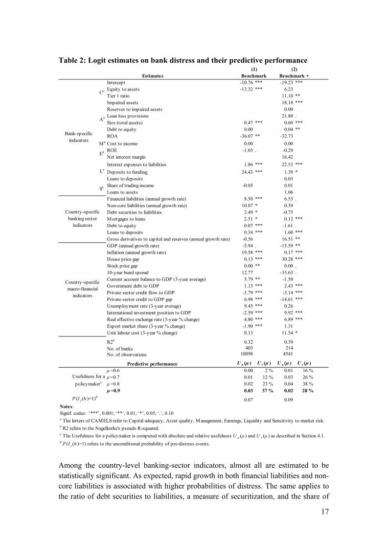
explanatory power. Second, the section discusses the predictive performance of the early-warning model. 5.1 Predicting Distress in European Banks We are interested in two key issues: what are the main sources of bank vulnerabilities and to what extent do indicators, or groups of them, predict bank vulnerabilities? Table 2 presents the estimates of the benchmark logit model, which predicts bank vulnerability 8 quarters ahead of distress. The coefficients refer to the estimation sample (2000Q1-2010Q1). The ending date is chosen as per the availability of full information on bank vulnerabilities. Yet, the predictions use recursive increasing windows for the in-sample data (2000Q1-2011Q4) and rolling windows for the out-of-sample data (2007Q1-2011Q4). The benchmark model (Model 1) contains vulnerability indicators that are drawn from the three groups introduced in Section 3: bank-level indicators, country-specific banking sector indicators and country-level macro-financial indicators. The model is chosen based on two considerations. On the one hand, the model should be encompassing and contain a wide-range of potential vulnerabilities. On the other hand, bank-specific items that have a comparatively short history in available data sources limit the number of observations. Model 2 (Benchmark+) in Table 2 presents results based on a trade-off between the number of observations and the number of indicators. Including the Tier 1 capital ratio, impaired assets, reserves to impaired assets and loan loss provisions reduces the number of available banks from 403 to 214 and the observations from 10,898 to 4,541, but does not improve the predictive usefulness of the model. Table 2 shows that most of the coefficients in the benchmark model are statistically significant. Among the bank-specific indicators, a high capital ratio and a high return on assets are associated with lower distress probabilities. High interest expenses and a high ratio of deposits-to-funding, on the other hand, increase the probability of distress. Generally, the signs of the coefficients follow economic intuition and findings in the literature, such as higher levels of bank capitalization decreasing distress probabilities, larger banks being more vulnerable, higher returns on equity lowering distress probabilities and larger funding costs increasing bank vulnerability. The positive sign of the deposits-to-funding ratio is the only somewhat counterintuitive estimate, as bank deposits are normally considered a more stable source of funding compared to wholesale funding sources (interbank borrowing or borrowing from capital markets).

17

Table 2: Logit estimates on bank distress and their predictive performance

Intercept -10.76 *** -19.23 ***Equity to assets -13.32 *** 6.23Tier 1 ratio 11.10 **Impaired assets 18.18 ***Reserves to impaired assets 0.00Loan loss provisions 21.80 .Size (total assets) 0.47 *** 0.60 ***Debt to equity 0.00 0.04 **ROA -36.07 ** -32.73

M a Cost to income 0.00 0.00ROE -1.03 . -0.29Net interest margin 16.42

Interest expenses to liabilities 1.86 *** 22.53 ***

Deposits to funding 24.43 *** 1.39 *Loans to deposits 0.03Share of trading income -0.05 0.01Loans to assets 1.06Financial liabilities (annual growth rate) 8.50 *** 6.53 .Non-core liabilities (annual growth rate) 10.07 * 0.39Debt securities to liabilities 2.49 * -0.75Mortgages to loans 2.51 * 0.12 ***Debt to equity 0.07 *** -1.61 .Loans to deposits 0.34 *** 1.60 ***Gross derivatives to capital and reserves (annual growth rate) -0.56 16.51 **GDP (annual growth rate) -5.94 . -15.59 **Inflation (annual growth rate) 19.58 *** 0.17 ***House price gap 0.13 *** 30.28 ***Stock price gap 0.00 ** 0.00 .10-year bund spread 12.77 -33.63 .Current account balance to GDP (3-year average) 5.79 ** -1.50Government debt to GDP 1.13 *** 2.43 ***Private sector credit flow to GDP -3.79 *** -3.14 ***Private sector credit to GDP gap 6.98 *** -14.61 ***Unemployment rate (3-year average) 9.45 *** 0.26International investment position to GDP -2.59 *** 9.92 ***Real effective exchange rate (3-year % change) 4.80 *** 6.89 ***Export market share (3-year % change) -1.90 *** 1.31Unit labour cost (3-year % change) 0.13 11.54 *

R2b 0.32 0.39No. of banks 403 214No. of observations 10898 4541

U a (μ ) U r (μ ) U a (μ ) U r (μ )

μ=0.6 0.00 2 % 0.01 16 %μ=0.7 0.01 12 % 0.03 26 %μ=0.8 0.02 23 % 0.04 38 %μ =0.9 0.03 37 % 0.02 28 %

P (I j (h )=1)d0.07 0.09

Sa

(1)Estimates Benchmark

(2)Benchmark +

Notes:Signif. codes: ‘***’, 0.001; ‘**’, 0.01; ‘*’, 0.05; ‘.’, 0.10a The letters of CAMELS refer to Capital adequacy, Asset quality, Management, Earnings, Liquidity and Sensitivity to market risk.b R2 refers to the Nagelkerke's pseudo R-squared.c The Usefulness for a policymaker is computed with absolute and relative usefulness U a (μ ) and U r (μ ) as described in Section 4.1.d P (I j (h )=1) refers to the unconditional probability of pre-distress events.

Bank-specific indicators

Country-specific banking sector

indicators

Country-specific macro-financial

indicators

Predictive performance

Usefulness for a

policymakerc

Ca

Aa

Ea

La

Among the country-level banking-sector indicators, almost all are estimated to be statistically significant. As expected, rapid growth in both financial liabilities and non-core liabilities is associated with higher probabilities of distress. The same applies to the ratio of debt securities to liabilities, a measure of securitization, and the share of

18

mortgages among loans, a proxy for property booms. Likewise, high banking system leverage and a high loans-to-deposits ratio increase bank vulnerability. Among the country-specific macro-financial indicators, all estimates have the expected sign. High inflation and low real GDP growth increase bank vulnerability. Likewise, positive stock and house price gaps that proxy for overvaluation of assets, increase distress probabilities. Regarding indicators of internal imbalances, the estimated coefficient for government debt is positive, whereas the estimated coefficient for private sector credit flow is negative and the coefficient for private sector credit-to-GDP gap is positive. This could be interpreted as an indication of bank vulnerability being increased when there is an ongoing credit contraction or credit crunch or when there are accumulated imbalances through a credit boom (credit-to-GDP gap). Higher levels of unemployment increase bank vulnerability. Finally, regarding external competitiveness, high net external borrowing of a country increases bank vulnerability, whereas a higher current account balance lowers bank vulnerability. This could be interpreted as the current account surplus proxying for a boom in an economy that increases the vulnerability of a bank. An increase in the real effective exchange rate and a decrease in export market share positively affect bank vulnerability through a loss of competitiveness. Table 2 also evaluates the predictive performance of the models based upon the recursive estimation procedure presented in Section 4.2 for each quarter in 2007Q1-2011Q4 (out-of-sample) conditional on the policymaker’s preference parameter

9.0,...,7.0,6.0 . Given that the threshold λ for classifying signals is a time-varying

parameter that is chosen to optimize in-sample usefulness at each t, the table does not report the applied λ. As discussed above, we assume that the policymaker is substantially more interested in correctly calling bank distress events than tranquil periods. This is intuitive if we consider that an early-warning signal triggers an in-depth review of fundamentals, business model and peers of the bank predicted to be in distress. Should the analysis reveal that the signal is false, there is no loss of credibility on behalf of the policy authority. Hence, in the benchmark case, preferences are set to 9.0 . Table 2 reports both the absolute and the relative

Usefulness measures as well as the unconditional probability of pre-distress events

(0.07). The benchmark model's absolute Usefulness aU equals 0.03 ( aU ) which

translates into a relative Usefulness rU equal to 37%, in contrast to rU equals to 28%

for Model 2 which includes a larger sample of bank-specific indicators. Table 3 provides information on the predictive power of the three indicator groups. Conditional on a preference parameter 9.0 , Model 4 based on macro-financial

indicators clearly outperforms the other models by achieving a rU of 24%. The

specification in column 2, which includes only bank-specific indicators, achieves a

19

rU of 16% compared to 2% for the banking-sector model. The comparison of rU

may be performed in terms of percentage points. That is, Model 2 generates 14 percentage points and Model 4 generates 22 percentage points more useful predictions than those of Model 3. It is, indeed, an interesting finding that macro-financial indicators turn out to be more useful for predicting vulnerabilities at the bank level than bank-specific indicators. However, the latest crisis clearly evolved along national borders. While the macro-financial indicators consist of those featured in the MIP, and have been chosen to mimic imbalances prior to this crisis, they follow the earlier literature on country-level imbalances (e.g., Demirgüç-Kunt and Detragiache, 1998; Kaminsky and Reinhart, 1999; Borio and Lowe, 2002). Models 5-6 not only confirm that combining the bank-level data with country-specific banking sector indicators generates little added value, but also the fact that combining bank-level data and macro-financial indicators produces a model that clearly outperforms a model with only bank-level data. As the benchmark model still improves predictive performance compared to that of Model 6, it is justified to use all three groups of indicators, also from a statistical point of view. Finally, Table 3 confirms the overall relative stability of the estimates and that in addition to the highest usefulness, the benchmark model also obtains the highest R2 (0.32). Table 4 shows the predictive performance of the benchmark model for different policymaker preferences between type I and II errors. The models are calibrated with

respect to non-weighted absolute Usefulness )(aU , but we also compute weighted

absolute Usefulness ),( ja wU for each preferences, where weights jw represent

bank size.6 The rationale for using absolute size, rather than bank size to the size of the country-specific banking sector, is the focus on systemically important financial institutions (SIFIs) in general, not domestic SIFIs. When focusing on non-weighted

)(aU , the results indicate that it is optimal to disregard the model for 5.0 . The

model derives negative )(aU for 5.0,4.0 as signalling for a tiny fraction of

bank-quarter observations yields )(aU in sample but not out of sample. For

3.0 , the policymaker is better off by not signalling at all. In addition, Table 4

shows that model performance decreases slightly for 9.0 when augmenting the

Usefulness measure with bank-specific weights ( ),( ja wU ). This would confirm the

expected effect as vulnerabilities and risks of large financial institutions are

oftentimes more complex than those of smaller ones. However, ),( ja wU is larger

than non-weighted for 8.0,3.0 . This is somewhat counterintuitive as the

estimates in Table 2 show that larger entities are more vulnerable to distress.

6 Systemic relevance of a bank is approximated by computing its share of total assets to total assets in the sample at quarter t. A possible amendment is to derive the systemic relevance from the systemic risk contributions of banks from, e.g., tail dependence networks.

20

Table 3: Logit estimates on bank distress and their predictive performance – models using different set of indicators

Intercept -10.76 *** -4.65 *** -5.35 *** -3.36 *** -6.02 *** -6.57 ***

Ca Equity to assets -13.32 *** -15.47 *** -13.68 *** -13.60 ***Size (total assets) 0.47 *** 0.38 *** 0.40 *** 0.47 ***Debt to equity 0.00 -0.01 . -0.01 0.00ROA -36.07 ** -16.34 -28.94 * -41.35 **

M a Cost to income 0.00 -0.01 0.00 0.00

Ea ROE -1.03 . -2.53 *** -2.15 *** -1.07 .

Interest expenses to liabilities 1.86 *** 2.61 *** 2.11 *** 1.53 ***Deposits to funding 24.43 *** 21.14 *** 20.80 *** 23.88 ***

Sa Share of trading income -0.05 -0.07 . -0.07 . -0.05Financial liabilities (annual growth rate) 8.50 *** 0.62 3.75 .Non-core liabilities (annual growth rate) 10.07 * 14.40 *** 12.47 ***Debt securities to liabilities 2.49 * -3.62 *** -2.04 **Mortgages to loans 2.51 * 7.56 *** 6.48 ***Debt to equity 0.07 *** 0.08 *** -0.03 *Loans to deposits 0.34 *** 0.26 *** 0.36 ***Gross derivatives to capital and reserves (annual growth rate) -0.56 -0.51 -1.06 *GDP (annual growth rate) -5.94 . -7.82 ** -5.77 .Inflation (annual growth rate) 19.58 *** 24.51 *** 18.87 ***House price gap 0.13 *** 0.10 *** 0.12 ***Stock price gap 0.00 ** 0.00 * 0.00 ***10-year bund spread 12.77 3.92 4.35Government debt to GDP 1.13 *** -0.61 * 0.26Private sector credit flow to GDP -3.79 *** -1.63 * -2.68 ***Private sector credit to GDP gap 6.98 *** 10.92 *** 7.76 ***Unemployment rate (3-year average) 9.45 *** 2.74 2.67Current account balance to GDP (3-year average) 5.79 ** 5.33 ** 8.51 ***International investment position to GDP -2.59 *** -1.41 *** -2.49 ***Real effective exchange rate (3-year % change) 4.80 *** 4.99 *** 4.88 ***Export market share (3-year % change) -1.90 *** -3.23 *** -2.53 ***Unit labour cost (3-year % change) 0.13 -4.57 ** 0.16

R2b 0.32 0.17 0.06 0.14 0.21 0.31No. of banks 403 403 403 403 403 403

U a (μ ) U r (μ ) U a (μ ) U r (μ ) U a (μ ) U r (μ ) U a (μ ) U r (μ ) U a (μ ) U r (μ ) U a (μ ) U r (μ )

μ=0.6 0.00 2 % 0.00 0 % 0.00 0 % 0.00 0 % 0.00 0 % 0.00 2 %μ=0.7 0.01 12 % 0.00 2 % 0.00 -1 % 0.00 -1 % 0.00 5 % 0.01 11 %μ=0.8 0.02 23 % 0.00 5 % 0.00 1 % 0.01 10 % 0.01 12 % 0.02 23 %μ =0.9 0.03 37 % 0.01 16 % 0.00 2 % 0.02 24 % 0.01 16 % 0.03 36 %

P (I j (h )=1)d0.07 0.07 0.07 0.07 0.07 0.07

(5)BS ModelEstimates

Aa

BSI Model(6)(1) (2) (3)

La

MF Model BS & MF ModelBS & BSI Model(4)

Bank-specific indicators

Country-specific banking sector

indicators

Country-specific macro-financial

indicators

Notes:Signif. codes: ‘***’, 0.001; ‘**’, 0.01; ‘*’, 0.05; ‘.’, 0.10a The letters of CAMELS refer to Capital adequacy, Asset quality, Management, Earnings, Liquidity and Sensitivity to market risk.b R2 refers to the Nagelkerke's pseudo R-squared.c The Usefulness for a policymaker is computed with absolute and relative usefulness U a (μ ) and U r (μ ) as described in Section 4.1.d P (I j (h )=1) refers to the unconditional probability of pre-distress events.

Usefulness for a

policymakerc

Benchmark

Predictive performance

21

Table 4: The predictive performance of the benchmark specification for different policymakers' preferences

Preferences Precision Recall Precision Recall Accuracy FP rate FN rate U a (μ ) U r (μ ) U a (μ ,w j U r (μ ,w j AUC

μ=0.0 0 0 5025 605 NA 0.00 0.89 1.00 0.89 0.00 1.00 0.00 NA 0.00 NA 0.80μ=0.1 0 0 5025 605 NA 0.00 0.89 1.00 0.89 0.00 1.00 0.00 0 % 0.00 0 % 0.80μ=0.2 0 0 5025 605 NA 0.00 0.89 1.00 0.89 0.00 1.00 0.00 0 % 0.00 0 % 0.80μ=0.3 0 0 5025 605 NA 0.00 0.89 1.00 0.89 0.00 1.00 0.00 0 % 0.00 1 % 0.80μ=0.4 20 26 4999 585 0.43 0.03 0.90 0.99 0.89 0.01 0.97 0.00 -3 % 0.01 6 % 0.80μ=0.5 78 91 4934 527 0.46 0.13 0.90 0.98 0.89 0.02 0.87 0.00 -2 % 0.01 11 % 0.80μ=0.6 119 161 4864 486 0.43 0.20 0.91 0.97 0.89 0.03 0.80 0.00 2 % 0.03 19 % 0.80μ=0.7 187 262 4763 418 0.42 0.31 0.92 0.95 0.88 0.05 0.69 0.01 12 % 0.06 32 % 0.80μ=0.8 243 414 4611 362 0.37 0.40 0.93 0.92 0.86 0.08 0.60 0.02 23 % 0.04 26 % 0.80μ =0.9 336 746 4279 269 0.31 0.56 0.94 0.85 0.82 0.15 0.44 0.03 37 % 0.01 16 % 0.80μ=1.0 605 5025 0 0 0.11 1.00 NA 0.00 0.11 1.00 0.00 0.00 NA 0.00 NA 0.80

Notes: The table reports results for real-time out-of-sample predictions of a logit model with optimal thresholds w.r.t. Usefulness with given preferences. Bold entries correspond to the benchmark preferences. Thresholds are calculated for μ={0.0,0.1,...,1.0} and the forecast horizon is 8 quarters. The table also reports in columns the following measures to assess the overall performance of the models: TP = True positives, FP = False positives, TN= True negatives, FN = False negatives, Precision positives = TP/(TP+FP), Recall positives = TP/(TP+FN), Precision negatives = TN/(TN+FN), Recall negatives = TN/(TN+FP), Accuracy =

(TP+TN)/(TP+TN+FP+FN), absolute and relative usefulness Ua and Ur (see formulae 1-3), and AUC = area under the ROC curve (TP rate to FP rate). See Section 4.1

for further details on the measures.

TP FP TN FN

Positives Negatives

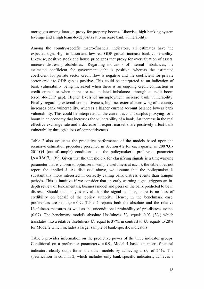
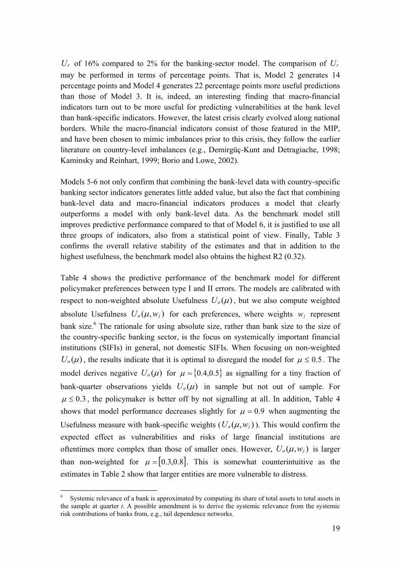
Figure 2 shows how the benchmark model would have performed out of sample in the case of Dexia from 2007Q1-2011Q4. The figure shows blue and green lines for absolute and percentile distress probabilities and highlights in grey the periods when the model signals. The black lines on top of the x-axis represent the distress events and the red lines the vulnerable states (or pre-distress) that the model aims to correctly call. In the run up to the first distress event in 2008, the model signals early on and consistently ranks Dexia as one of the most risky banks in the sample (as shown by the percentile probabilities). Later, the model is not quite as successful, though it correctly signals the first quarters of vulnerability and a couple of quarters before the second distress event. Figure 3 shows a similar case study on Bank of Ireland. The model signals vulnerability in 2007Q4, when the distress event occurs in 2009Q1, and throughout the pre-distress period before the distress event that started in 2010Q2.

Absolute distress probabilitiesPercentile distress probabilitiesEarly warning signals

Dexia SA

2007 Q1 2007 Q3 2008 Q1 2008 Q3 2009 Q1 2009 Q3 2010 Q1 2010 Q3 2011 Q1 2011 Q3

0.0

0.2

0.4

0.6

0.8

1.0

Pre-distress event Distress event

Figure 2: A case study of the early-warning model on Dexia. Out-of-sample prediction of bank distress (8 quarters ahead) from 2007Q1-2011Q4.

22

Absolute distress probabilitiesPercentile distress probabilitiesEarly warning signals

Bank of Ireland

2007 Q1 2007 Q3 2008 Q1 2008 Q3 2009 Q1 2009 Q3 2010 Q1 2010 Q3 2011 Q1 2011 Q3

0.0

0.2

0.4

0.6

0.8

1.0

Pre-distress event Distress event

Figure 3: A case study of the early-warning model on Bank of Ireland. Out-of-sample prediction of bank distress (8 quarters ahead) from 2007Q1-2011Q4.

6. Robustness We test the robustness of the early-warning model in several ways. As Table 2 shows, the results are, in a broad sense, robust to omitting some key CAMELS indicators with weak data coverage, such as Tier 1 capital ratio, loan loss provisions and impaired assets. Similarly, Table 3 showed that complementing bank-specific vulnerabilities with indicators of macro-financial imbalances is crucial for model performance, while the predictive performance is not sensitive to excluding indicators of imbalances in countries' banking-sectors. Further, as partly discussed in the Section 5 (Tables 2,3 and 4), the out-of-sample performance of the model is sensitive to the policymaker’s preferences due to the unbalanced frequencies of distress events and tranquil periods. For a model to be useful, this motivates preferences of 5.0 . In addition, we study the out-of-sample performance for different forecast horizons. As shown in Table 5, the absolute Usefulness of the model improves when the out-of-sample forecast horizon increases from 12 months to 24 months, whereas the performance for horizons of 24 and 36 months is similar. The models' relative Usefulness is, however, similar for different horizons. This is mainly due to the fact that increases in unconditional probabilities of pre-distress events also raise the Usefulness of the models, as the loss of disregarding a model increases.

23

Table 5: Robustness of the model with respect to out-of-sample forecast horizon ForecastHorizon Precision Recall Precision Recall Accuracy FP rate FN rate U a (μ ) U r (μ ) U a (μ ,w j U r (μ ,w j AUC

12 months 94 193 1871 67 0.33 0.58 0.97 0.91 0.88 0.09 0.42 0.03 45 % 0.02 31 % 0.7624 months 336 746 4279 269 0.31 0.56 0.94 0.85 0.82 0.15 0.44 0.03 37 % 0.02 29 % 0.8036 months 237 527 1376 85 0.31 0.74 0.94 0.72 0.72 0.28 0.26 0.03 32 % 0.03 31 % 0.86

Notes: The table reports results for real-time out-of-sample predictions of a logit model with optimal thresholds w.r.t. Usefulness with given preferences. Bold entries correspond to the benchmark horizon and thresholds are calculated for μ={0.0,0.1,...,1.0}. The table also reports in columns the following measures to assess the overall performance of the models: TP = True positives, FP = False positives, TN= True negatives, FN = False negatives, Precision positives = TP/(TP+FP), Recall positives =

TP/(TP+FN), Precision negatives = TN/(TN+FN), Recall negatives = TN/(TN+FP), Accuracy = (TP+TN)/(TP+TN+FP+FN), absolute and relative usefulness Ua and Ur

(see formulae 1-3), and AUC = area under the ROC curve (TP rate to FP rate). See Section 4.1 for further details on the measures.

Negatives

TP FP TN FN

Positives

Finally, we show the sensitivity of the early-warning model to variation of the thresholds with an ROC curve. The curve plots the benefit (true positive rate) to the cost (false positive rate) of a certain model for each threshold λ, as noted in Section 4.1. While not accounting for imbalanced data and misclassification costs, the ROC curve's area above the diagonal line represents the benefit of a model in relation to a coin toss. Figure 4 not only shows that the ROC curves are above those of a coin toss, but also that curves of 24 and 36-month horizons are similar, while that of a 12-month horizon is somewhat poorer. This exercise is, however, somewhat imprecise. While the models issue signals based upon time-varying thresholds such that in-sample Usefulness is optimized, the ROC statistics treat all probabilities as similar. Another common limitation of the ROC curve, especially the AUC, is that parts of it, which are not policy relevant, are included in the computed area.

0 0.2 0.4 0.6 0.8 1

0

0.2

0.4

0.6

0.8

1

FP rate

TP

rate

h = 12 monthsh = 24 monthsh = 36 months

Figure 4: Robustness of the model with respect to λ for different forecast horizons

24

7. Conclusions

The paper presents an early-warning model for predicting bank distress in the European banking sector, using both bank-level and country-level indicators of vulnerabilities, and introduces a novel dataset of bank distress events. As outright bank failures have been rare in Europe, we introduce a novel dataset that complements bankruptcies, liquidations and defaults by also taking into account state interventions, and mergers in distress. Moreover, the signals of the early-warning model are calibrated not only according to policymakers' preferences between type I and II errors, but also accounting for the potential systemic relevance of each individual financial institution, proxied by its size. The paper finds that complementing bank-specific vulnerabilities with indicators for macro-financial imbalances improves model performance. Thus, the results in this paper confirm the usefulness of the vulnerability indicators introduced recently via the EU Macroeconomic Imbalance Procedure (MIP). In addition, the results show that an early-warning model based on publicly available data yields useful out-of-sample predictions of bank distress during the current financial crisis (2007Q1-2011Q4). Finally, the results of the evaluation framework show that a policymaker has to be substantially more concerned of missing bank distress than issuing false alarms for the model to be useful. This is intuitive if we consider that an early-warning signal triggers an in-depth review of fundamentals, business model and peers of the bank predicted to be in distress. Should the analysis reveal that the signal is false, there is no loss of credibility on behalf of the policy authority. The evaluations also imply that it is important to give more emphasis to systemically important and large banks for a policymaker concerned with systemic risk.

25

References

Agarwal, V. and R. Taffler. (2008). "Comparing the performance of market-based and accounting-based bankruptcy prediction models." Journal of Banking & Finance 32(8), pp. 1541–1551.

Alessi, L. and C., Detken. (2011). "Quasi real time early warning indicators for costly asset price boom/bust cycles: A role for global liquidity." European Journal of Political Economy 27(3), 520–533.

Berg, A. and C., Pattillo (1999a). "Predicting Currency Crises: The Indicators Approach and an Alternative." Journal of International Money and Finance 18(4), 561–586.

Berg, A., and C., Pattillo. (1999b). "What caused the Asian crises: An early warning system approach." Economic Notes 28, 285–334.

van den Berg, J., B., Candelon, J. Urbain. (2008). "A cautious note on the use of panel models to predict financial crises." Economics Letters 101(1), 80-83.

Bharath, S.T., and T., Shumway. (2008). "Forecasting default with the Merton distance to default model." The Review of Financial Studies 21, 1339–1369.

Borio, C. and P., Lowe. (2002). "Asset Prices, Financial and Monetary Stability: Exploring the Nexus." BIS Working Papers, No. 114, Bank for International Settlements, July 2002.

Bussière, M. and M., Fratzscher. (2008). "Low probability, high impact: Policy making and extreme events.” Journal of Policy Modeling 30, 111–121.

Bussière, M., and M. Fratzscher. (2006). "Towards a new early warning system of financial crises." Journal of International Money and Finance 25(6), 953–973.

Campbell, J., J., Hilscher and J., Szilagyi. (2008). "In search of distress risk." The Journal of Finance 58(6), 2899–2939.

Cole, R. A., and J.W., Gunther. (1995). "Separating the likelihood and timing of bank failure." Journal of Banking and Finance 19, 1073–1089.

Cole, R., and J.W., Gunther. (1998). "Predicting bank failures: A comparison of on- and off-site monitoring systems." Journal of Financial Services Research 13(2), 103–117.

Curry, T., P., Elmer and G., Fissel. (2007). "Equity market data, bank failures and market efficiency." Journal of Economics and Business 59, 536–559.

Davis E.P. and D., Karim. (2008a). "Could Early Warning Systems Have Helped To Predict the Sub-Prime Crisis?." National Institute Economic Review 206(1), 35–47.

26

Davis, E.P. and D., Karim. (2008b). "Comparing Early Warning Systems for Banking Crisis." Journal of Financial Stability 4(2), 89–120.

Dell'Ariccia, G., E. Detragiache and R. Rajan. (2008). "The Real Effects of Banking Crises." Journal of Financial Intermediation 17, 89–112.

Demirgüç-Kunt, A. and E., Detragiache. (1998). "The determinants of banking crises in developed and developing countries." IMF Staff Papers 45(1), 81–109.

Demirgüç-Kunt, A. and E., Detragiache. (2000). "Monitoring Banking Sector Fragility. A Multivariate Logit." World Bank Economic Review 14(2), 287–307.

EC. (2012). "Scoreboard for the surveillance of macroeconomic imbalances." European Economy Occasional Papers 92, European Commission, February 2012.

Edison, H.J. (2003). "Do Indicators of Financial Crises Work? An Evaluation of an Early Warning System." International Journal of Finance & Economics 8(1), 11–53.

Flannery, M.J. (1998). "Using Market Information in Prudential Bank Supervision: A Review of the US Empirical Evidence." Journal of Money, Credit and Banking 30(3), 273–305

Frankel, J. and A., Rose. (1996). "Currency Crashes in Emerging Markets: An Empirical Treatment." Journal of International Economics 41(3–4), 351–366.

Fuertes, A.-M., E., Kalotychou. (2006). "Early Warning System for Sovereign Debt Crisis: the role of heterogeneity." Computational Statistics and Data Analysis 5, 1420–1441.

Fuertes, A.M., E., Kalotychou. (2007). "Towards the optimal design of an early warning system for sovereign debt crises." International Journal of Forecasting 23(1), 85–100.

González-Hermosillo, B. (1999). "Determinants of Ex-Ante Banking System Distress: A Macro-Micro Empirical Exploration of Some Recent Episodes." IMF Working Paper 99/33, International Monetary Fund, March 1999.

Hutchinson, M.M. (2002). "European Banking Distress and EMU: Institutional and Macroeconomic Risks." Scandinavian Journal of Economics 104(3), 365–389.

IMF. (2010). "The IMF-FSB Early Warning Exercise – Design and Methodological Toolkit." IMF Occasional Paper 10/274, International Monetary Fund September 2010.

Jagtiani, J. and C., Lemieux. (2001). "Market discipline prior to bank failure." Journal of Economics and Business 53, 313–324.

27

Jordá, O., M., Schularick and A.M., Taylor. (2011). "Financial Crises, Credit Booms, and External Imbalances: 140 Years of Lessons." IMF Economic Review 59(2), 340–378.

Kaminsky, G. and C.M., Reinhart. (1999). "The Twin Crises: The Causes of Banking and Balance-of-Payments Problems." American Economic Review 89(3), 473–500.

Kaminsky, G. (1998). "Currency and Banking Crises: The Early Warnings of Distress." International Finance Discussion Paper 629, Board of Governors of the Federal Reserve System, October 1998.

Kaminsky, G., S., Lizondo and C.M., Reinhart. (1998). "Leading Indicators of Currency Crises." IMF Staff Papers 45(1), 1–48.

Kumar, M., Moorthy, U., Perraudin, W. (2003). "Predicting emerging market currency crashes." Journal of Empirical Finance 10, 427–454.

Laeven, L. and F., Valencia. (2008). "Systemic Banking Crises: A New Database." IMF Working Paper 08/224, International Monetary Fund, November 2008.

Laeven, L. and F., Valencia. (2010). "Resolution of Banking Crises: The Good, the Bad, and the Ugly." IMF Working Paper 10/146, International Monetary Fund, June 2010.

Laeven, L. and F., Valencia. (2011). "The Real Effects of Financial Sector Interventions During Crises." IMF Working Paper 11/45, International Monetary Fund, March 2011.

Männasoo, K., D.G., Mayes. (2009). "Explaining bank distress in Eastern European transition economies." Journal of Banking and Finance 33(2), 244–253

Mody, A. and D., Sandri. (2012). "The Eurozone Crisis: How Banks and Sovereigns Came to Be Joined at the Hip." Economic Policy 27(70), 199–230.

Ötker, I and J., Podpiera. (2010). "The Fundamental Determinants of Credit Default Risk for European Large Complex Financial Institutions." IMF Working Paper 10/153, International Monetary Fund, June 2010.

Poghosyan, T. and M., Cihák. (2011). "Distress in European Banks: An Analysis Based on a New Dataset." Journal of Financial Services Research 40 (3), 163–184

Reinhart, C.M. and K.S., Rogoff. (2008). "Is the 2007 US Sub-Prime Financial Crisis So Different? An International Historical Comparison." American Economic Review 98(2), 339–344.

Reinhart, C.M. and K.S., Rogoff. (2009). "The Aftermath of Financial Crises." American Economic Review 99(2), 466–472.

28

Rose, A.K. and M.M., Spiegel. (2011). "Cross-country causes and consequences of the crisis: An update." European Economic Review 55(3), 309–324.

Sarlin, P. and T.A., Peltonen, 2011, Mapping the State of Financial Stability, ECB Working Paper No. 1382, European Central Bank, September 2011.

Sarlin, P. (2012). "On policymakers' loss functions and the evaluation of early warning systems." TUCS Technical Report No. 1054, Turku Centre for Computer Science, June 2012.

Schularick, M. and A.M., Taylor. (2011). "Credit Booms Gone Bust: Monetary Policy, Leverage Cycles and Financial Crises, 1870–2008." American Economic Review 102(2), 1029–1061.

Sun, T. (2011). "Identifying Vulnerabilities in Systemically-Important Financial Institutions in a Macrofinancial Linkages Framework." IMF Working Paper 11/111, International Monetary Fund, May 2011.

Whalen, G. (1991). "A Proportional Hazards Model of Bank Failure: An Examination of Its Usefulness as an Early Warning Tool." Federal Reserve Bank of Cleveland Economic Review Q1, 21–31.

Thomson, J. (1992). "Modeling the regulator’s closure option: A two-step logit regression approach." Journal of Financial Services Research 6, 5–23.

Appendices Table A: Indicators, definitions, transformations and data sources

Variable Definition and transformation SourceInterceptEquity to assets Total Equity / Total Assets BloombergTier 1 ratio Tier 1 Capital Ratio BloombergImpaired assets Non Performing Assets / Total Assets BloombergReserves to impaired assets Reserves for Loan Losses / Non Performing Assets BloombergLoan loss provisions Provisions for Loan Losses / Total Average Loans BloombergSize (total assets) Natural logarithm of Total Assets BloombergDebt to equity Total Liabilities / Total Equity BloombergROA Return on Assets Bloomberg

M Cost to income Operating Costs / Operating Income BloombergROE Return on Equity BloombergNet interest margin Net Interest Margin BloombergInterest expenses to liabilities Interest Expenses / Total Liabilities BloombergDeposits to funding Deposits / Funding BloombergLoans to deposits Total Loans / Customer Deposits BloombergShare of trading income Trading Income / Operating Income BloombergLoans to assets Total Loans / Total Assets BloombergFinancial liabilities (annual growth rate) Growth rate of (Total Assets - Capital and Reserves) ECB MFI statisticsNon-core liabilities (annual growth rate) Growth rate of (Total Liabilities - Capital and Reserves - Deposits) ECB MFI statisticsDebt securities to liabilities Debt securities to liabilities ECB MFI statisticsMortgages to loans Mortgages to Total Loans ECB MFI statisticsDebt to equity ( Total Liabilities - Capital and Reserves ) / Capital and Reserves ECB MFI statisticsLoans to deposits Total Loans / Deposits ECB MFI statisticsGross derivatives to capital and reserves (annual growth rate) Growth rate of ((Positive Derivatives + Negative Derivatives) / Capital and ReseECB MFI statisticsGDP (annual growth rate) Growth rate of real GDP EurostatInflation (annual growth rate) Growth rate of HICP index EurostatHouse price gap House price index - HP filtered trend ECBStock price gap Stock price index - HP filtered trend Bloomberg10-year bond spread Long-term government bond yield - German long-term government bond yield BloombergGovernment debt to GDP General government debt as % of GDP Eurostat / Alert Mechanism ReportPrivate sector credit flow to GDP Private sector credit flow as % of GDP Eurostat / Alert Mechanism ReportPrivate sector credit to GDP gap Moving sum of 4 quarters of private sector credit / GDP - HP filtered trend Haver Analytics / IMF IFSUnemployment rate (3-year average) 3 year average of unemployment rate Eurostat / Alert Mechanism ReportCurrent account balance to GDP (3-year average) 3 year average of current account balance as a % of GDP Eurostat / Alert Mechanism ReportInternational investment position to GDP Net International Investment Position as a % of GDP Eurostat / Alert Mechanism ReportReal effective exchange rate (3-year % change) % change (3 years) of Real Effective Exchange Rate, HICP deflators relative Eurostat / Alert Mechanism ReportExport market share (3-year % change) % change (5 years) in export market shares Eurostat / Alert Mechanism ReportUnit labour cost (3-year % change) % change (3 years) in nominal unit labour cost Eurostat / Alert Mechanism Report

L

S

Country-specific

banking sector variables

Country-specific macro-

financial variables

Bank-specific balance-

sheet variables

C

A

E

30

Table B: Summary statistics Variables Obs Min Max Mean Std. Dev. Skew KurtEquity to assets 15773 0.01 0.35 0.07 0.05 3.01 14.38Tier 1 ratio 8759 0.05 0.31 0.10 0.04 2.28 7.35Impaired assets 9111 0.00 0.14 0.02 0.03 2.10 5.11Reserves to impaired assets 8672 0.00 48.59 1.96 5.83 7.29 54.08Loan loss provisions 12040 0.00 0.07 0.01 0.01 3.63 16.55Size (total assets) 15962 -0.15 7.14 3.02 1.82 0.44 -0.70Debt to equity 15718 0.44 74.40 18.10 12.51 2.12 5.86ROA 15886 -0.04 0.03 0.01 0.01 -1.25 8.75

M a Cost to income 15452 -32.08 38.78 2.50 6.85 0.13 15.62ROE 15646 -0.78 0.36 0.07 0.14 -3.48 18.53Net interest margin 12466 0.00 0.07 0.02 0.01 1.19 2.77Interest expenses to liabilities 15139 0.00 0.11 0.03 0.02 2.03 5.78Deposits to funding 14880 0.00 0.97 0.54 0.24 -0.34 -0.55Loans to deposits 13408 0.06 19.41 1.92 2.55 5.23 30.10Share of trading income 15078 -5.46 5.44 0.23 1.05 -0.48 15.79Loans to assets 13868 0.00 0.93 0.61 0.21 -1.01 0.70Financial liabilities (annual growth rate) 24706 -0.14 0.22 0.02 0.03 0.39 3.41Non-core liabilities (annual growth rate) 24706 -0.25 0.11 0.00 0.01 -0.23 22.96Debt securities to liabilities 24767 0.00 0.51 0.17 0.09 0.68 2.03Mortgages to loans 24627 0.01 0.41 0.17 0.07 0.62 0.16Debt to equity 24767 3.87 28.12 14.50 4.17 0.59 -0.48Loans to deposits 24767 1.00 7.42 2.42 0.78 1.84 6.25Gross derivatives to capital and reserves (annual growth rate) 24566 -0.50 1.70 0.01 0.12 3.51 29.80GDP (annual growth rate) 25449 -0.18 0.16 0.02 0.03 -0.95 2.68Inflation (annual growth rate) 25529 -0.07 0.54 0.02 0.02 8.44 179.89House price gap 22620 -26.59 34.09 0.00 3.63 0.77 14.40Stock price gap 25399 -18825.03 24098.27 41.28 3187.38 0.48 6.9410-year bund spread 25082 -0.01 0.32 0.01 0.02 9.77 145.20Current account balance to GDP (3-year average) 25529 -0.22 0.11 -0.01 0.04 -0.17 0.36Government debt to GDP 25529 0.04 1.65 0.71 0.28 0.30 -0.57Private sector credit flow to GDP 25529 -0.59 1.62 0.09 0.11 2.91 48.03Private sector credit to GDP gap 26098 -0.27 0.33 0.00 0.04 1.34 6.83Unemployment rate (3-year average) 25529 0.02 0.20 0.08 0.03 1.19 2.65International investment position to GDP 25529 -1.48 1.40 -0.19 0.36 0.02 1.62Real effective exchange rate (3-year % change) 25529 -0.20 0.38 0.01 0.06 -0.10 2.37Export market share (3-year % change) 25529 -0.24 0.78 -0.05 0.15 2.11 5.83

Unit labour cost (3-year % change) 25529 -0.17 1.39 0.07 0.06 5.28 93.74Notes: The statist ics are derived from the entire sample with 26,852 observations.a The letters refer to Capital Adequacy (C), Asset Quality (A), Management (M), Earnings (E), Liquidity (L), and Sensitivity to Market Risk (S)

Country-specific macro-financial

indicators

Bank-specific

indicators

Ca

Aa

Ea

La

Sa

Country-specific banking sector

indicators

31

Table C: Mean-comparison tests

Variables Obs Mean Std. Dev. Obs Mean Std. Dev. t Prob

Equity to assets 14987 0.07 0.05 786 0.05 0.03 16.42 0.00

Tier 1 ratio 8226 0.10 0.04 533 0.09 0.02 14.78 0.00

Impaired assets 8585 0.02 0.03 526 0.03 0.03 3.55 0.00

Reserves to impaired assets 8170 2.02 5.97 502 1.01 2.74 7.33 0.00

Loan loss provisions 11404 0.01 0.01 636 0.01 0.01 6.40 0.00

Size (total assets) 15176 2.96 1.81 786 4.11 1.69 18.58 0.00

Debt to equity 14932 17.76 12.25 786 24.64 15.35 12.36 0.00

ROA 15101 0.01 0.01 785 0.00 0.01 10.99 0.00

M a Cost to income 14675 2.51 6.85 777 2.28 6.85 0.91 0.36

ROE 14861 0.07 0.13 785 0.00 0.25 8.30 0.00

Net interest margin 11806 0.02 0.01 660 0.02 0.01 2.29 0.02

Interest expenses to liabilities 14390 0.03 0.02 749 0.04 0.02 10.41 0.00

Deposits to funding 14133 0.54 0.24 747 0.53 0.23 1.76 0.08

Loans to deposits 12711 1.92 2.57 697 1.91 2.21 0.17 0.00

Share of trading income 14330 0.23 1.03 748 0.23 1.40 0.05 0.87

Loans to assets 13151 0.61 0.21 717 0.59 0.19 3.51 0.96

Financial liabilities (annual growth rate) 23714 0.02 0.03 992 0.02 0.03 1.05 0.29Non-core liabilities (annual growth rate) 23714 0.00 0.01 992 0.00 0.01 3.32 0.00

Debt securities to liabilities 23775 0.17 0.09 992 0.16 0.10 4.58 0.00

Mortgages to loans 23635 0.17 0.07 992 0.20 0.07 15.52 0.00

Debt to equity 23775 14.48 4.18 992 14.86 3.85 2.99 0.00

Loans to deposits 23775 2.42 0.77 992 2.43 1.04 0.45 0.65

Gross derivatives to capital and reserves (annual growth rate) 23574 0.01 0.12 992 0.01 0.11 0.71 0.48GDP (annual growth rate) 24449 0.02 0.03 1000 0.00 0.03 13.06 0.00

Inflation (annual growth rate) 24529 0.02 0.02 1000 0.02 0.02 0.51 0.61House price gap 21703 -0.07 3.59 917 1.57 4.15 11.79 0.00

Stock price gap 24399 43.49 3232.20 1000 -12.73 1772.05 0.94 0.35

10-year bund spread 24106 0.01 0.02 976 0.01 0.02 3.09 0.00

Current account balance to GDP (3-year average) 24529 -0.01 0.04 1000 -0.03 0.06 12.78 0.00

Government debt to GDP 24529 0.71 0.28 1000 0.64 0.26 8.63 0.00

Private sector credit flow to GDP 24529 0.09 0.11 1000 0.10 0.11 2.29 0.02

Private sector credit to GDP gap 25109 0.00 0.04 989 0.04 0.07 15.36 0.00

Unemployment rate (3-year average) 24529 0.08 0.03 1000 0.09 0.04 2.66 0.01

International investment position to GDP 24529 -0.18 0.35 1000 -0.43 0.47 16.50 0.00

Real effective exchange rate (3-year % change) 24529 0.01 0.06 1000 0.02 0.05 5.96 0.00

Export market share (3-year % change) 24529 -0.05 0.16 1000 -0.08 0.10 12.07 0.00

Unit labour cost (3-year % change) 24529 0.06 0.06 1000 0.08 0.08 6.17 0.00

Sa

Notes: The statistics are derived from the entire sample with 26,852 observations. C = 0 refers to tranquil periods and C = 1to vulnerable states (pre-distress periods). a The letters refer to Capital Adequacy (C), Asset Quality (A), Management (M), Earnings (E), Liquidity (L), and Sensitivity to Market Risk (S)

Country-specific banking sector

indicators

C = 0 C = 1 Mean t -test

Bank-specific

indicators

Country-specific macro-financial

indicators

Ca

Aa

Ea

La