predicting corrosion on protected buried steel natural gas
TRANSCRIPT

Predicting Corrosion on Protected Buried Steel Natural GasDistribution Pipelines
ByLillian Ruth Meyer
B.S., Civil Engineering, Rice University, 2012
Submitted to the MIT Sloan School of Management and the Department of Civil Engineering in partial
fulfillment of the requirements for the degrees ofMaster of Business Administration MASSACHUSET
and OF TECH
Master of Science in Civil Engineeringin conjunction with the Leaders for Global Operations Program at the JUN 0
MASSACHUSETTS INSTITUTE OF TECHNOLOGYJune 2016 LIBRA
0 2016 Lillian Ruth Meyer. All rights reserved.
The author hereby grants to MIT permission to reproduce and to distribute publicly paper and electronic copies of
this thesis document in whole or in part in any medium now known or hereafter created.
Signature redactedA uthor........................................................ ....... . ....... ---... . . . . .---------
MIT Sloan School of Management and Department of Civil & Environmental EngineeringMay 6, 2016
Signature redactedCertified bv ........
Georgia Perakis, Thesis SupervisorWilliams F. Pound Professor of Management, MIT Sloan School of Management
C ertified by ..........................................
Professor, D
A pproved by..........................................
Director,
A pproved by.......................................
Signature redactedHerbert H. Einstein, Thesis Supervisor
epartment of Civil and Environmental Engineering-- 1/ P/
Signature redactedV V - - Maur-aTerson'-
MBA Program, vIT Sloan School of Management
i r 1 /1-/ 1
Sianature redactedI I
ieidi Nepf
Donald and Martha Harleman Professor of Civil and Environmental 1lngineeringChair, Graduate Program Committee
S IN TUTENOLOGY
7 2016
RIES
. .. . .. .

THIS PAGE INTENTIONALLY LEFT BLANK
2
Predicting Corrosion on Protected Buried Steel Natural Gas
Distribution Pipelines
By
Lillian Ruth Meyer
Submitted to the Department of Civil Engineering and the MIT Sloan School of Management on
May 6, 2016, in partial fulfillment of the requirements for the degrees ofMaster of Science in Civil Engineering
andMaster of Business Administration
Abstract
PG&E uses cathodic protection, which connects the pipeline to sacrificial anodes that corrode instead of
the pipeline, to prevent corrosion on its buried steel natural gas pipelines. However, corrosion leaks still
occur. This thesis focuses on whether corrosion leaks can be predicted on steel distribution natural gas
pipeline that is cathodically protected. By proactively understanding where leaks are most likely to occur
rather than examining past leak performance, PG&E can better optimize its resources to reduce the risk of
corrosion on its pipeline.
We introduced logistic regression to model whether or not a corrosion leak will occur in a cathodic
protection area, a one to ten mile length of pipe that uses the same corrosion control equipment. Two
different types of data were available: data that are relatively static and data that are relatively dynamic
with respect to time. We built two different sets of logistic regression models to examine two questions:
(1) if data from one area can be used to predict where corrosion leaks will occur in another area; and (2) if
data from one year can be used to predict where corrosion leaks will occur during the following year. The
models for both questions use cross-validation to test the influence on model accuracy of the in-sample
and out-of-sample data sets.
The first model addresses the first question by using pipe characteristic and soil data with a mean average
percentage error ranging from 35% to 96%. The significant factors in a given cathodic protection area
(CPA) that consistently drive the model include: length of steel main pipe; percent of steel main pipe
designated as low pressure; the average moist bulk density of the soil; the variation of soil pH; average
clay content in the soil; variation of clay content in the soil; and the average saturated hydraulic
conductivity of the soil. The second model addresses the second question by using the previous year's
routine maintenance and weather data with a mean average percentage error ranging from 40% to 81%.
The significant factors in a given CPA that consistently drive the model include: the length of steel main
pipe and average temperature.
Thesis Supervisor: Herbert H. EinsteinTitle: Professor, Department of Civil & Environmental Engineering
Thesis Supervisor: Georgia PerakisTitle: Williams F. Pound Professor of Management, MIT Sloan School of Management
3

THIS PAGE INTENTIONALLY LEFT BLANK
4

Acknowledgements
This project would not exist without the support of Pacific Gas and Electric Company. I thank
Preston Ford, Sumeet Singh, and Mallik Angalakudati for providing guidance and advice that
enabled this project's success.
Additionally, I thank my thesis advisors, Professor Herbert Einstein and Professor Georgia
Perakis. Your insights and recommendations have been extraordinarily valuable. This thesis is
greatly improved because of your involvement.
Thanks to the LGO office for their guidance. I would also like to acknowledge my LGOclassmates. I leave MIT and LGO a better person because of you all.
Finally, many thanks to my family for your constant love and support. Without you, I could not
have achieved so much.
5

THIS PAGE INTENTIONALLY LEFT BLANK
6
Table of Contents
A bstract..................................................................................................................................... 3
A cknow ledgem ents......................................................................................................................... 5
Table of Contents.......................................................................................................................... 7
Chapter 1: Introduction................................................................................................................ 10
1.1 Problem Statem ent............................................................................................................ 10
1.2 Hypothesis and Project M otivation ............................................................................... 11
1.3 M ain Contributions........................................................................................................... 12
1.4 Thesis Overview ............................................................................................................... 12
Chapter 2: Problem Background and Literature Review ............................................................. 14
2.1 Corrosion .......................................................................................................................... 14
2.2 Pipeline Industry Standard Corrosion Control M ethods ............................................... 16
2.3 Estim ates of Corrosion Rates ........................................................................................ 19
2.4 Statistical M ethods to Estim ate Corrosion Rates .......................................................... 21
2.5 Evaluating Cathodic Protection on Buried Steel Pipelines .......................................... 21
Chapter 3: Hypothesis, M odeling Approach, and D ata........................................................... 24
3.1 Questions and a Hypothesis........................................................................................... 24
3.2 The D ependent V ariable ............................................................................................... 25
3.3 M odeling A pproach...................................................................................................... 25
3.4 D ata................................................................................................................................... 29
3.5 M etrics for M easuring M odel Perform ance ................................................................. 39
3.5 Sum m ary........................................................................................................................... 42
Chapter 4: Results ........................................................................................................................ 43
4.1 Significant Static Independent Variables ..................................................................... 43
4.2 Significant Dynam ic Independent Variables ................................................................. 49
4.3 Com paring the Tw o M odels .......................................................................................... 52
4.4 Sum m ary........................................................................................................................... 54
Chapter 5: Conclusions................................................................................................................ 56
5.1 Sum m ary of Results...................................................................................................... 56
5.2 Recom m endations for Future W ork ............................................................................... 57
7
A pp en d ix ................................................................................................................ .. ... ------.... 5 9
A B ib lio grap hy ....................................................................................................................... 59
B Commonly Used Abbreviations ..................................................................................... 61
List of Figures
F igure 1: Basic corrosion cell ................................................................................................. 15
Figure 2: Steel pipe with cathodic protection........................................................................... 17
Figure 3: Galvanic cathodic protection (reproduced from Uhlig's Corrosion Handbook) ........ 17
Figure 4: Impressed current cathodic protection (reproduced from Uhlig's Corrosion
H a n d bo o k).............................................................................................................................--.-... 18
Figure 5: Schematic of modeling process - regression models ............................................... 26
Figure 6: Schematic of regression models............................................................................... 27
Figure 7: Schematic of modeling process - data...................................................................... 30
Figure 8: Minimum versus maximum daily temperatures ........................................................ 34
Figure 9: Hierarchy of USDA web soil survey area designations .......................................... 36
Figure 10: Properties within a soil map unit........................................................................... 37
F igure J] : Soil p rop erties............................................................................................................ 38
Figure 12: Schematic of modeling process - cross-validation runs......................................... 40
Figure 13: Example RO C curve .............................................................................................. 41
Figure 14: Histogram ofpressure type in for each cross-validation in-sample data set ........ 46
Figure 15: Histogram ofpressure type in for each cross-validation in-sample data set ........ 47
Figure 16: Histograms of current density within CPAs for each cross-validation in-sample data
set .................................................................................................... .......... ... . .. ----................. 5 1
Figure] 7: ROC curves for the static model............................................................................. 52
Figure 18: ROC curves for the dynamic model ........................................................................ 53
8
List of Tables
Table ]: Various corrosion cells..................................................................................................
Table 2: D uration of corrosion on 2-inch diameter steel pipe ....................................................
Table 3: ECDA data elements (reproduced from ANSI/NACE SP 0502-2010) ..........................
Table 4: Performance of dynam ic data using various models ....................................................
Table 5: Pipe diameter ranges considered ..................................................................................
Table 6: Sign ficant factors for static model................................................................................
Table 7. Significant factors for dynamic model...........................................................................
Table 8: Fit of data to logistic regressions ..................................................................................
Table 9: Error measurements ......................................................................................................
9
15
20
22
29
36
44
50
53
54
Chapter 1: Introduction
1.1 Problem Statement
Corrosion and its consequences are pervasive problems for natural gas and water utilities, and
other transmission pipelines throughout the United States. Two recent high profile failures due
to corrosion in water pipelines have highlighted the potentially disastrous consequences of
corrosion. The first example is the corrosion of the lead water distribution pipes in Flint,
Michigan due to the lack of corrosion controls causing lead contamination in the water. After
switching to drawing water from the Flint River as a cost-saving measure, no corrosion control
plan was put in place to prevent the more corrosive water from damaging the water pipeline.
[1]. The second example is the leak in an 8-inch thick concrete water pipeline in Santa Clara
County in August 2015. A crack in the mortar on the outside of the pipe allowed water to seep
in and corrode the steel and concrete of the pipe walls. It cost $1.2 million to repair the pipe and
the estimated cost of inspecting and repairing the nearby pipe is at least $6.8 million [2]. These
two instances highlight how costly corrosion failures can be when infrastructure is not properly
protected and monitored.
Natural gas provides about 25% of the United States' energy [3]. Three different types of
pipeline systems carry natural gas from production wells to the final point of use such as homes
and businesses. First, gathering pipelines carry natural gas from production wells. Second,
transmission pipelines carry natural gas over thousands of miles across the country, closer to the
communities that will use this product. Third, distribution pipelines carry natural gas into
communities and bring it to its point-of-use. Distribution mains are the larger pipes that carry
the natural gas through cities and neighborhoods while services carry the natural gas from the
main directly into homes and businesses [4].
Corrosion is a naturally occurring process in which a material degrades. About 35% of leaks
repaired on distribution main natural gas pipe in the United States are due to corrosion [5].
These corrosion leaks occur despite 89% of all steel gas distribution main being reported as
cathodically protected. Cathodic protection is the industry standard method of controlling
corrosion on steel pipelines. Essentially, another metal (called a sacrificial anode) is linked to
the pipeline system. This metal corrodes instead of the valuable steel pipeline asset.
10
Pacific Gas and Electric Company (PG&E) has one of the largest natural gas networks in the
United States. The utility serves over 15 million people in Northern and Central California and
has 4.3 million gas accounts. It has approximately 48,000 miles of gas pipeline. 6,700 miles are
high pressure transmission pipelines and 42,000 miles of distribution pipelines. 21,000 miles of
the distribution pipe is steel and susceptible to corrosion [6]. This thesis focuses on a subset of
those 21,000 miles of steel distribution pipe.
Similar to the rest of the industry, despite the application of cathodic protection, corrosion leaks
still occur on PG&E's system. PG&E has increased its focus on finding and identifying
corrosion leaks in its distribution system. However, with a gas pipeline network as large as
PG&E's, this task becomes complicated. Ideally, the areas most at-risk from corrosion (both in
terms of probability of corrosion and consequences of corrosion) are identified and monitored
before areas with less corrosion risk.
PG&E reviews historical leak data to identify the areas with the highest number of corrosion
leaks. These areas are investigated to find the root causes for the corrosion leaks. However, the
cause of a leak is not identified until the leak is repaired. Hence, when PG&E investigates root
causes of leaks, the conditions that initially caused the leaks may have already been corrected. Is
there a method that considers future performance of corrosion controls and the pipeline system to
identify areas most at risk from corrosion rather than considering past performance of the
pipeline system?
1.2 Hypothesis and Project Motivation
This thesis investigates if statistical regressions can predict where corrosion leaks are most likely
to occur on PG&E's distribution network and identifies factors related to the nature of the pipe,
the corrosion control, or the environment that may affect corrosion of cathodically protected steel
pipe. By identifying the factors that most significantly affect the likelihood of corrosion, PG&E
could work proactively to improve its corrosion controls and prevent corrosion from occurring
on its distribution pipe. Furthermore, PG&E could identify parts of its system that are most at
risk from corrosion and better optimize its resources to monitor and improve those parts in order
to decrease the risk from corrosion.
11
1.3 Main Contributions
We introduced two predictive models built using logistic regressions to answer the questions: 1)
can we predict where corrosion is most likely to occur in an area using data from another area
and 2) can we predict where corrosion is most likely to occur in a given year using another data
from the previous year. Two types of data were available: data that remained relatively the
same over time (static data) and data that changed over time (dynamic data). We created two
predictive models since, if we created one single model using both the static and dynamic data,
that model would not be truly out-of-sample. We would have used the same data to build the
model as to test the model's predictive ability.
The predictive model that answers the first question is referred to as the static model while the
predictive model that answers the second question is referred to as the dynamic model. The
mean average percentage errors for the static model ranges from 35% to 96%. The mean
average percentage errors for the dynamic model ranges from 40% to 81%.
1.4 Thesis Overview
Chapter 2 presents the project background including descriptions of corrosion and industry
standard corrosion control practices. Additionally, Chapter 2 reviews current literature about
corrosion rates on steel with various levels of cathodic protection and statistical methods used to
estimate corrosion rates. Finally, it discusses a current industry standard practice, the External
Corrosion Direct Assessment, for examining where corrosion is occurring and to what extent.
As will be discussed in Chapter 2, while corrosion rates and the External Corrosion Direct
Assessment provide ways to measure corrosion, both require excavating the pipe. The steel pipe
needs to be excavated in order to validate the corrosion rates and to perform the External
Corrosion Direct Assessment. Excavating the steel pipe is a costly and disruptive process
according to the population density of the neighborhood of interest. Using corrosion leaks as a
measure of performance for the corrosion controls on the system removes the need for
excavation but is a retroactive measure of performance.
This thesis develops two different methods to predict if corrosion leaks are likely to occur in a
given area of steel pipe. Using predictive models allows PG&E to identify the areas most at risk
12

from corrosion and target those areas with additional resources in order to proactively reduce the
risk.
Chapter 3 identifies the questions that are answered by the predictive models. Given the
available data: can we predict (1) where corrosion is most likely to occur in an area using data
from another area and (2) where corrosion is most likely to occur in a given year using data from
the previous year. Chapter 3 also discusses in further detail why corrosion leaks (and
specifically corrosion leaks repaired) are the best measurement of corrosion occurrence in a
given area. We examine several different regression models (linear, quasi-Poisson, logistic, and
random forest). Since logistic regression has the lowest error when predicting corrosion, it is the
regression used to build the predictive models. Two predictive models were built because the
available data contained both data that changed over time (dynamic data) and data that remained
relatively static over time (static data). Section 3.4 describes this data in further detail. We also
identify metrics for measuring performance of the models.
Chapter 4 describes the results for both the static and dynamic models. First, the significant
independent variables for each of the static and dynamic models are discussed. Additionally, we
compare the performance of the static and dynamic models against each other. The dynamic
model both fits the data better and more accurately predicts if corrosion leaks will occur.
Chapter 5 presents the conclusions drawn from the predictive models and provides
recommendations for future work. Commonly used abbreviations are defined in Appendix B.
13
Chapter 2: Problem Background and Literature Review
This literature review first discusses the corrosion process. Next, it explains current corrosion
control methods and the history of these methods. Then, it describes different corrosion rates of
steel and the expected time before corrosion causes leaks on the pipeline system. Additionally, it
discusses various statistical methods used to estimate the initiation and growth of corrosion.
Finally, it discusses the industry standard practice of external corrosion direct assessments on
steel pipe, a current method of identifying how corrosion affects the integrity of the pipeline
system.
2.1 Corrosion
[7] and [8] detail the theory behind corrosion. Corrosion is a process during which a material
degrades. For metal, corrosion occurs naturally over time as the metal transitions from a high-
energy state after its extraction from the earth to a lower-energy (and more stable) state. Two
electrochemical reactions describe corrosion: an anodic (or oxidation) reaction or a cathodic (or
reduction) reaction. Equation 1 is the typical anodic reaction while Equations 2a and 2b are the
cathodic reactions that occur in oxygen or water, respectively. Essentially, the anodic reaction is
the "donation" of electrons from one area to another while the cathodic reaction is
complementary the "collection" electrons.
(1) Fe-+Fe2+2e- anodic reaction
(2a) 02+2H2O+4e--*40H- oxygen cathodic reaction
(2b) 2H20+2e--H 2+2OH water cathodic reaction
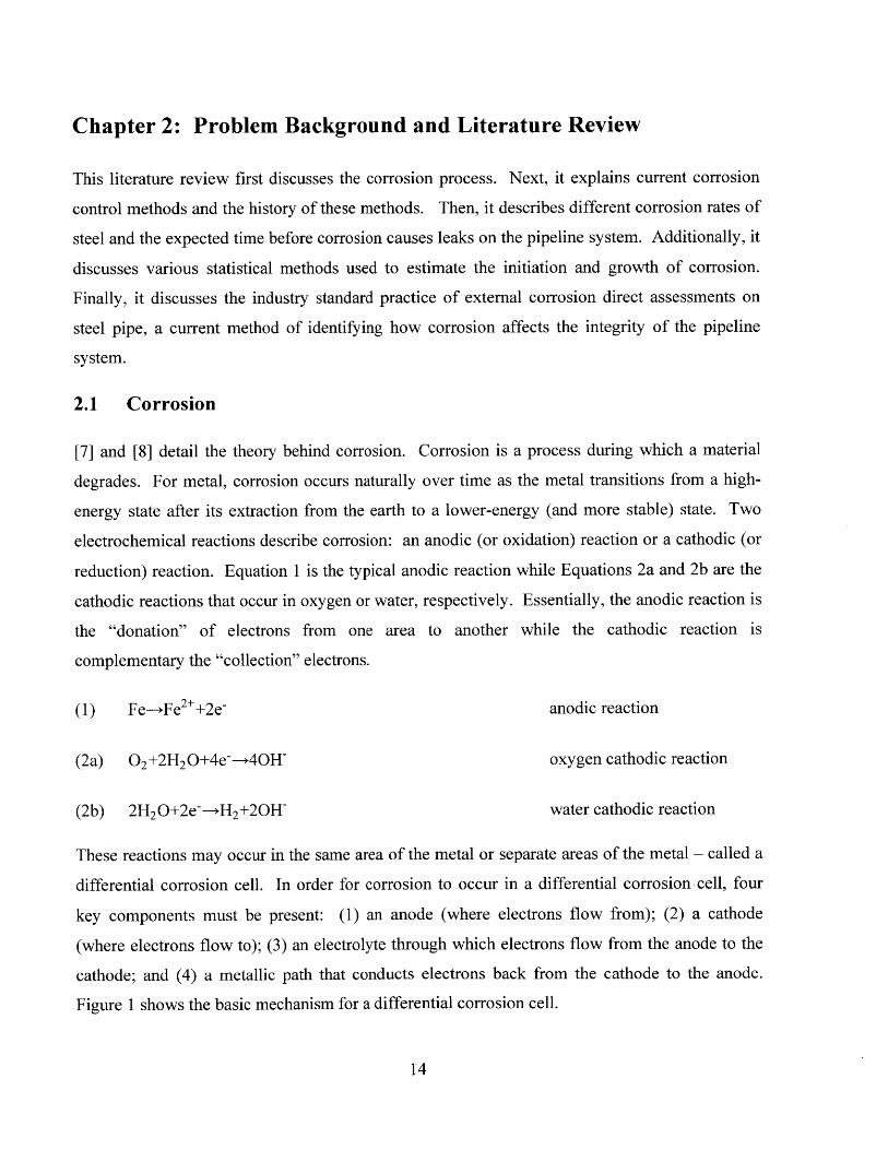
These reactions may occur in the same area of the metal or separate areas of the metal - called a
differential corrosion cell. In order for corrosion to occur in a differential corrosion cell, four
key components must be present: (1) an anode (where electrons flow from); (2) a cathode
(where electrons flow to); (3) an electrolyte through which electrons flow from the anode to the
cathode; and (4) a metallic path that conducts electrons back from the cathode to the anode.
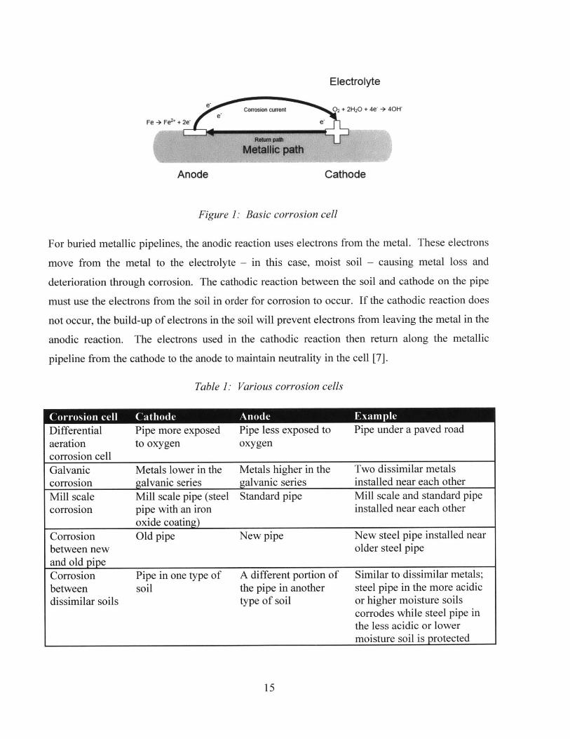
Figure 1 shows the basic mechanism for a differential corrosion cell.
14
Electrolyte
e Corrosion current 0, + 2H 20 + 4e' + 40H^e
Fe + Fe2 + 2e
Return pat
Metallic path
Anode Cathode
Figure 1: Basic corrosion cell
For buried metallic pipelines, the anodic reaction uses electrons from the metal. These electrons
move from the metal to the electrolyte - in this case, moist soil - causing metal loss and
deterioration through corrosion. The cathodic reaction between the soil and cathode on the pipe
must use the electrons from the soil in order for corrosion to occur. If the cathodic reaction does
not occur, the build-up of electrons in the soil will prevent electrons from leaving the metal in the
anodic reaction. The electrons used in the cathodic reaction then return along the metallic
pipeline from the cathode to the anode to maintain neutrality in the cell [7].
Table 1: Various corrosion cells
Differential Pipe more exposed Pipe less exposed to Pipe under a paved roadaeration to oxygen oxygencorrosion cellGalvanic Metals lower in the Metals higher in the Two dissimilar metalscorrosion galvanic series galvanic series installed near each otherMill scale Mill scale pipe (steel Standard pipe Mill scale and standard pipecorrosion pipe with an iron installed near each other
oxide coating)Corrosion Old pipe New pipe New steel pipe installed nearbetween new older steel pipeand old pipeCorrosion Pipe in one type of A different portion of Similar to dissimilar metals;between soil the pipe in another steel pipe in the more acidicdissimilar soils type of soil or higher moisture soils
corrodes while steel pipe inthe less acidic or lowermoisture soil is protected
15
There are several types of corrosion cells that can trigger the flow of electrons. Table 1 presents
various corrosion cells and brief descriptions of the process [7].
2.2 Pipeline Industry Standard Corrosion Control Methods
There are two primary methods of controlling corrosion on steel pipelines: coatings and cathodic
protection. Used together, coatings and cathodic protection can effectively prevent corrosion
from occurring. The Pipeline and Hazardous Materials Safety Administration (PHMSA) - the
federal regulatory agency for natural gas pipelines - requires that all pipelines installed after
July 31, 1971 have coatings and cathodic protection [9].
Coatings
Coatings act as insulation and prevent the anodic and cathodic reactions (i.e. the electrons from
moving between the pipe and soil). The application of coatings during pipe installation started in
the 1930s and became more prevalent by the 1940s. By the 1950s, most pipes were installed
with coatings [10]. In the industry, coal tar and asphalt enamel were used as early coating
materials before the 1960s. In the 1960s through 1980s, polyethylene tape and fusion bonded
epoxies were developed and used as coating materials [10]. It is practically infeasible to have a
pipe perfectly protected by coatings since holes and nicks in coatings occur during and after
construction. The industry has focused on improvements in application and installation
techniques to minimize these imperfections in coatings [10]. Properly and effectively applied
coatings can protect 99% of the pipe from corrosion [7].
Cathodic protection
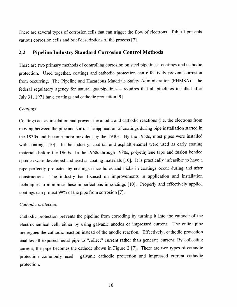
Cathodic protection prevents the pipeline from corroding by turning it into the cathode of the
electrochemical cell, either by using galvanic anodes or impressed current. The entire pipe
undergoes the cathodic reaction instead of the anodic reaction. Effectively, cathodic protection
enables all exposed metal pipe to "collect" current rather than generate current. By collecting
current, the pipe becomes the cathode shown in Figure 2 [7]. There are two types of cathodic
protection commonly used: galvanic cathodic protection and impressed current cathodic
protection.
16
Sacrificialanode Electrolyte
Protective current
Cathode, protected steel pipe
Figure 2: Steel pipe with cathodic protection
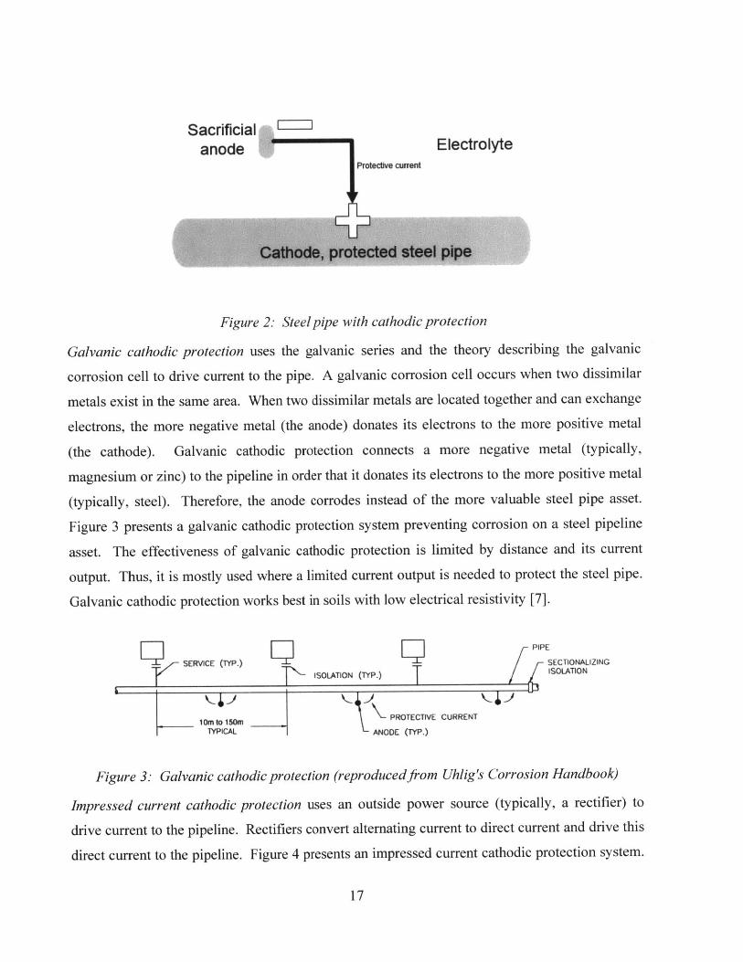
Galvanic cathodic protection uses the galvanic series and the theory describing the galvanic
corrosion cell to drive current to the pipe. A galvanic corrosion cell occurs when two dissimilar
metals exist in the same area. When two dissimilar metals are located together and can exchange
electrons, the more negative metal (the anode) donates its electrons to the more positive metal
(the cathode). Galvanic cathodic protection connects a more negative metal (typically,
magnesium or zinc) to the pipeline in order that it donates its electrons to the more positive metal
(typically, steel). Therefore, the anode corrodes instead of the more valuable steel pipe asset.
Figure 3 presents a galvanic cathodic protection system preventing corrosion on a steel pipeline
asset. The effectiveness of galvanic cathodic protection is limited by distance and its current
output. Thus, it is mostly used where a limited current output is needed to protect the steel pipe.
Galvanic cathodic protection works best in soils with low electrical resistivity [7].
E PIPE
SERVICE (TYP.) SEC I IONALIZING
ISOLATION (TYP.) ISOLATION
10io15om PROTECTIVE CURRENT
TYPICAL ANODE (TYP.)
Figure 3: Galvanic cathodic protection (reproduced fron Uhlig's Corrosion Handbook)
hnpressed current cathodic protection uses an outside power source (typically, a rectifier) to
drive current to the pipeline. Rectifiers convert alternating current to direct current and drive this
direct current to the pipeline. Figure 4 presents an impressed current cathodic protection system.
17
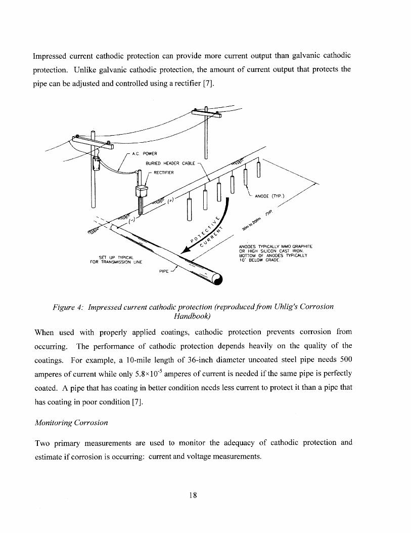
Impressed current cathodic protection can provide more current output than galvanic cathodic
protection. Unlike galvanic cathodic protection, the amount of current output that protects the
pipe can be adjusted and controlled using a rectifier [7].
BURIED HEADER CABLE
ANODE (TYP.)
ANODES TYPICALLY MMO GRAPHITEOR HIGH SILICON CAST IRON.
SET UP TYPICAL BOTTOM OF ANODES TYPICALLY
FOR TRANSMISSION LINE 10' BELOW GRADE.
PIPE
Figure 4: Impressed current cathodic protection (reproduced from Uhlig's CorrosionHandbook)
When used with properly applied coatings, cathodic protection prevents corrosion from
occurring. The performance of cathodic protection depends heavily on the quality of the
coatings. For example, a 10-mile length of 36-inch diameter uncoated steel pipe needs 500
amperes of current while only 5.8x 10- amperes of current is needed if the same pipe is perfectly
coated. A pipe that has coating in better condition needs less current to protect it than a pipe that
has coating in poor condition [7].
Monitoring Corrosion
Two primary measurements are used to monitor the adequacy of cathodic protection and
estimate if corrosion is occurring: current and voltage measurements.
18

Current measurements monitor the required current output in amperes from rectifiers necessary
to protect the pipe from corrosion. If the measured current output needed to protect the pipe
increases, the measured output increase can indicate the condition of the coatings or other issues
occurring in the system [7]. Uhlig's Corrosion Handbook presents typical current requirements
of 4.5 to 16.0 milliamperes per square meter of pipe when cathodically protecting bare steel in
neutral soil. Steel pipe with coatings will require a smaller amount of current. In more
corrosion-prone soil (well-aerated, highly acidic, with more sulfate-reducing bacteria, or higher
temperature), this current requirement can increase up to 450 milliamperes per square meter of
pipe [11]. A deviation in the measured current output from what is normally required can
indicate an issue with the rectifier or that the rectifier is protecting more than just the pipe (e.g. a
bicycle resting against a steel riser attached to the pipe).
Voltage measurements between the pipe and the soil (referred to as pipe-to-soil readings or P/S
readings) are also used to indicate if cathodic protection is adequate. This measurement checks
that the soil (and other objects) around the pipe is more negative than the pipe so that the pipe is
protected from local corrosion. There are three primary pipe-to-soil reading criteria used in
industry: (1) a pipe-to-soil reading equal to or more negative than -850 millivolts while cathodic
protection is applied; (2) a pipe-to-soil reading equal to or more negative than -850 millivolts
immediately after turning off rectifiers (interrupting the current flow for the pipe); or (3) a
polarization of 100 millivolts between the native potential of the steel pipe and the pipe-to-soil
reading just after turning off rectifiers (interrupting the current sources) [7].
Both the current and voltage measurements are useful to identify if the protective current is being
diverted from the cathodically protected pipe. When this occurs, the pipe may become
inadequately protected and corrosion can occur.
2.3 Estimates of Corrosion Rates
Various corrosion rates have been specified to estimate how fast corrosion occurs on buried
metals. The American National Standards Institute (ANSI) / National Association of Corrosion
Engineers (NACE) Standard Practice 0502-2010 Pipeline External Corrosion Direct Assessment
(ECDA) Methodology recommends using a pitting rate of at least 0.4 millimeters per year for
bare and unprotected buried steel. A corrosion pit is an area of the pipe where corrosion has
19

started to occur. The pitting rate estimates how fast the pit grows. If the cathodic protection has
been applied on the pipeline for a significant period of time, then the pitting rate may decrease
24% to 0.31 millimeters per year [12].
Barbalet et al. investigated the residual corrosion rate on buried steel pipe protected with
coatings and cathodic protection. They estimated residual corrosion rates ranging between 0.01
to 0.07 millimeters per year [13].
Table 2 summarizes the ECDA and Barbalet et al. corrosion rates. Additionally, it provides an
estimate of how long a 2-inch diameter steel pipe will corrode at those rates before for a leak
occurs. A standard 2-inch diameter steel pipe has a wall thickness of approximately 0.154 inches
(or 3.9 millimeters). When corrosion occurs, the wall thickness of the pipe decreases until
corrosion is either stopped by effective corrosion controls or until the wall thickness decreases
completely. This duration ranges from 10 years for no protection to 560 years if the pipe is
sufficiently protected using cathodic protection. If the pipe is insufficiently protected, then
assuming corrosion occurs at a constant rate, it will take 50 years for the pipe to develop a leak
after corrosion starts. Note that corrosion does not start immediately once the pipe is unprotected
or insufficiently protected. If corrosion does start immediately, then pipe that became
insufficiently protected in 1966 will develop corrosion leaks in 2016 per these rates.
Table 2: Duration of corrosion on 2-inch diameter steel pipe
Level of Protection Corrosion Rate Duration of Corrosion
(millimeters per year) (years)
No protection 0.4 10Insufficient protection 0.08 50Sufficient protection 0.007 560
The Caltrans Highway Design Manual estimates the years to perforation of steel culverts that
have 1.32-millimeter thick walls based on the minimum soil resistivity, R, and the soil pH.
Perforation refers to a hole developing in the wall of the culvert due to corrosion. This estimate
is presented in Equations 3a and 3b. In general, the corrosion occurs faster as soil resistivity and
soil pH decrease [14].
20

(3a) Years = 1.47 R 0,4
(3b) Years = 13.79 [Logio R - Logio (2160 - 2490 Logio pH)] for soil pH < 7.3
2.4 Statistical Methods to Estimate Corrosion Rates
Valor et al. describe stochastic models that describe corrosion pit initiation and growth. As
mentioned previously, a corrosion pit is an area of the pipe where corrosion is occurring. Pit
initiation is when the corrosion pit starts. Pit growth is the rate at which the area corrodes. Pit
initiation is typically modeled as nonhomogeneous Poisson process because a corrosion pit on an
unprotected pipe may start randomly. The time to the start of a corrosion pit (the pit initiation
time) typically follows a Weibull distribution (an extreme value distribution). Pit growth is
modeled using a non-homogeneous Markov model [15].
Caleyo et al. use Monte Carlo simulations to estimate the pitting rate and the average maximum
pit depth in various soils with various coating types. Their results indicate that the corrosion
rates described in the previous section are conservative for cathodically protected steel pipes
with coatings. The three extreme value distributions fit both the pitting rate and the average
maximum pit depth. The authors note that the corrosion rate varies most over a short period of
exposure time. The corrosion rate remains relatively constant after the pipe has been corroding
for a longer time [16].
2.5 Evaluating Cathodic Protection on Buried Steel Pipelines
[12] details the standard practice for performing external corrosion direct assessments (ECDA).
The purpose of an ECDA is to provide a structured process in order to assess the consequence of
external corrosion on a pipeline system. This process consists of four steps: 1) a pre-assessment,
2) an indirect assessment, 3) a direct inspection, and 4) a post-assessment.
The pre-assessment determines the practicality of an ECDA by collecting and reviewing data
relating to pipe, construction, environmental, corrosion control and operational factors. The data
involved in the pre-assessment step of the ECDA informed the data collection process for this
thesis. Table 3 presents the data used in the pre-assessment step of the ECDA. Items in bold
indicate data elements that were used in this thesis. Soil types and characteristics includes
21
for soil pH > 7.3
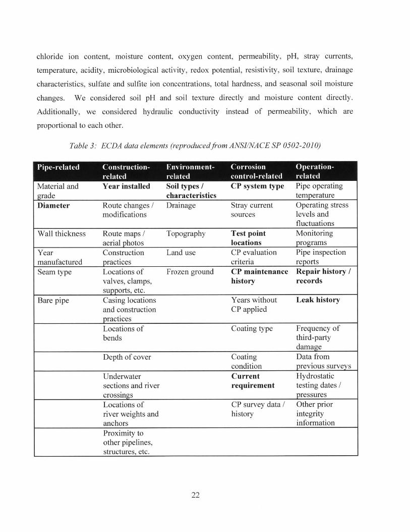
chloride ion content, moisture content, oxygen content, permeability, pH, stray currents,
temperature, acidity, microbiological activity, redox potential, resistivity, soil texture, drainage
characteristics, sulfate and sulfite ion concentrations, total hardness., and seasonal soil moisture
changes. We considered soil pH and soil texture directly and moisture content directly.
Additionally, we considered hydraulic conductivity instead of permeability, which are
proportional to each other.
Table 3: ECDA data elements (reproduced from ANSI/NACE SP 0502-2010)
Material and Year installed Soil types / CP system type Pipe operatinggrade characteristics temperatureDiameter Route changes / Drainage Stray current Operating stress
modifications sources levels andfluctuations
Wall thickness Route maps / Topography Test point Monitoringaerial photos locations programs
Year Construction Land use CP evaluation Pipe inspectionmanufactured practices criteria reportsSeam type Locations of Frozen ground CP maintenance Repair history /
valves, clamps, history recordssupports, etc.
Bare pipe Casing locations Years without Leak historyand construction CP appliedpracticesLocations of Coating type Frequency ofbends third-party
damageDepth of cover Coating Data from
condition previous surveysUnderwater Current Hydrostaticsections and river requirement testing dates /crossings pressuresLocations of CP survey data / Other priorriver weights and history integrityanchors informationProximity toother pipelines,structures, etc.
22
The indirect inspection is an aboveground survey that collects physical evidence in order to
estimate the degree of corrosion activity and coating damage to the pipe. The direct examination
uses the information from the pre-assessment and indirect inspection to identify locations to
physically excavate the pipe and examine visually. The post-assessment evaluates the ECDA
process and determines the schedule for re-assessments [12].
Corrosion rates describe how quickly we expect corrosion to cause a leak once corrosion starts.
However, the rates are meaningless when trying to evaluate the effectiveness of corrosion
controls on a pipeline system without uncovering the pipes and measuring the rate. This process
can be costly and disruptive. The ECDA process identifies areas where corrosion may be
occurring. However, the ECDA process is localized and does not unite all the elements of
corrosion and corrosion control in such a way that they can be evaluated across the entire
distribution system. The statistical models discussed in the next chapter can be used to describe
underlying trends throughout the entire system where corrosion is occurring without needing to
physically examine the pipe.
23
Chapter 3: Hypothesis, Modeling Approach, and Data
None of the methods described in the previous literature review chapter provide economical
ways to study the underlying causes of insufficient cathodic protection and corrosion leaks on a
natural gas distribution pipeline system. While the statistical modeling of pit growth and pit
initiation help examine the process of corrosion, it requires expensive and potentially disruptive
excavations to validate on a steel distribution pipeline in the field. Additionally, the External
Corrosion Direct Assessment (ECDA) also refers to past performance of the pipeline system
rather than considering future performance when identifying areas for further study of corrosion
and its effects on the pipeline integrity. This chapter again addresses why a model to predict the
occurrence of corrosion on a distribution system is important and presents a modeling approach
and the data available to do so.
3.1 Questions and a Hypothesis
Ensuring that a distribution gas system as large as PG&E's is sufficiently protected using
cathodic protection requires a tremendous amount of resources. As the utilities industry in
general notes an increasing issue with corrosion, two questions arise: 1) can insufficient
performance of cathodic protection be predicted and 2) can significant factors contributing to this
insufficient cathodic protection be identified? Using predictive models to understand where
insufficient cathodic protection is resulting in corrosion leaks and what factors are causing
insufficient cathodic protection can help inform additional proactive maintenance procedures
above industry standards and help PG&E to optimize its resources so that it can reduce risk in
the most corrosion-prone areas.
Insufficient performance of cathodic protection can be predicted and significant factors
contributing to this insufficient cathodic protection can be identified. Specifically, we can use
available operational, pipe, and environmental data to predict: (1) where corrosion is most likely
to occur in an area using data from another area and (2) where corrosion is most likely to occur
in a given year using data from the previous year. The rest of this chapter describes the
dependent variable and the modeling approach. Additionally, the available data and hypotheses
about how the available data influence the performance of cathodic protection are presented.
24
3.2 The Dependent Variable
This study uses the number of corrosion leaks repaired within a given area as the dependent
variable instead of a more direct measure of insufficient cathodic protection for three reasons.
First, the exact moment that cathodic protection performs insufficiently is ambiguous. Second, it
is economically infeasible to identify when the corrosion process actually begins since the
evidence of corrosion is not evident at the ground surface until a leak develops. Third, it is not
possible to know with confidence what causes a leak until the pipe is uncovered and examined.
This examination does not occur until the pipe is uncovered for repair. It is this leaks repaired
metric that is reported in the PHMSA Annual Report [5]. Hence, the number of leaks repaired
due to corrosion measures the occurrence of corrosion. The dependent variable for the models
presented in this thesis is the number of leaks repaired due to corrosion.
For the rest of this thesis, insufficient performance of cathodic protection, corrosion leaks
repaired, and corrosion occurrence are used interchangeably. The author recognizes that this
mingles different issues but due to the three reasons discussed above, corrosion leaks repaired is
the best available inference of insufficient cathodic protection and, therefore, corrosion
occurrence.
3.3 Modeling Approach
Figure 5 is a schematic describing the modeling process. The top row, in orange, shows the four
different regressions that were considered using the available data: simple linear regression,
quasi-Poisson regression, logistic regression, and random forest regression. Each regression type
is described briefly below. The linear, quasi-Poisson, and random forest regressions predict the
number of corrosion leaks that occur in a given CPA in a year; the logistic regression predicts
whether or not at least one corrosion leak will occur in a given CPA in a year. The second row
in Figure 5 lists the two data groups (static and dynamic) and the data that each group considers.
Although not indicated in Figure 5 for simplicity, the data groups are the same for each of the
regression models. In order to examine the effect of the in-sample data on the model results, we
used cross-validation. The bottom row indicates this cross-validation process. For the static
data, the areas of interest were subdivided into four groups by geographical area. Three groups
were used as the in-sample data to build the model in one cross-validation run while the fourth
25
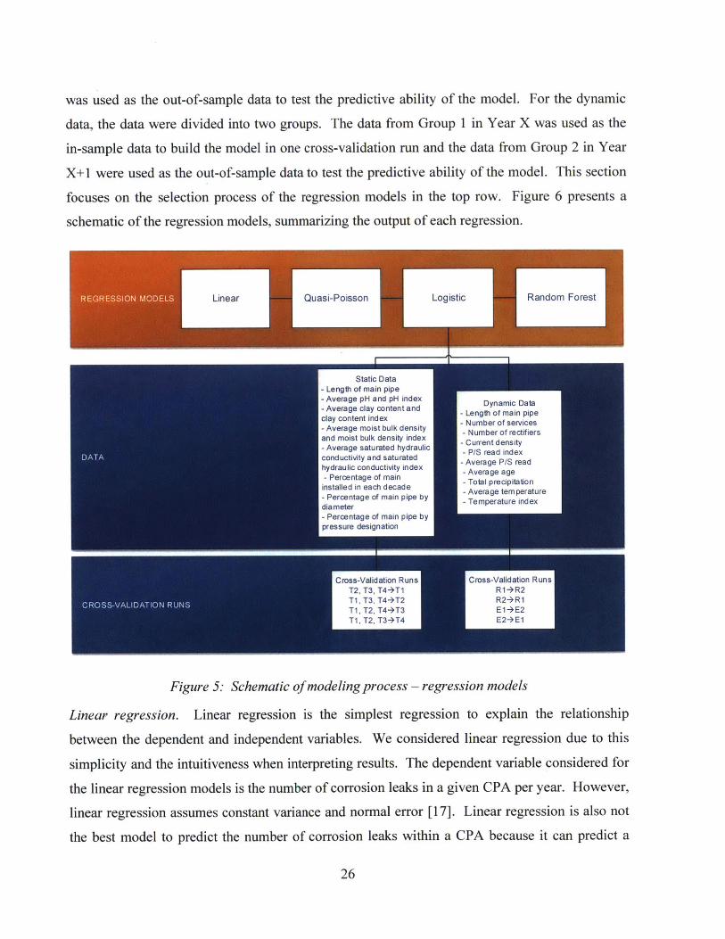
was used as the out-of-sample data to test the predictive ability of the model. For the dynamic
data, the data were divided into two groups. The data from Group I in Year X was used as the
in-sample data to build the model in one cross-validation run and the data from Group 2 in Year
X+1 were used as the out-of-sample data to test the predictive ability of the model. This section
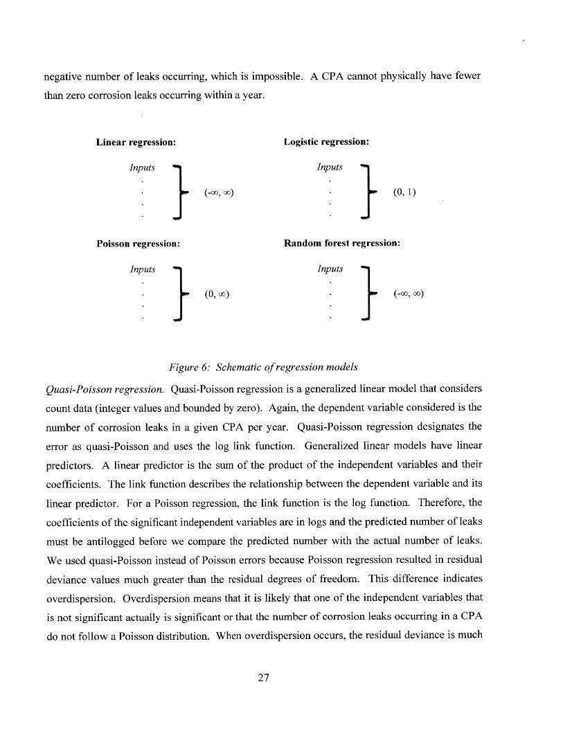
focuses on the selection process of the regression models in the top row. Figure 6 presents a
schematic of the regression models, summarizing the output of each regression.
LierQuasi-Poisson 7Logistic Rnom Forest
Static Data- Length of main pipe
Average pH and pH index Dynamic DataF Average clay content and g Length of main pipeclay content index -Number of services- Average moist bulk density Number of rectifieresand moist bulk density index - nCurrent density
a . Average saturated hydraulic - P/S read indexconductivity and saturated -Average P/S readhydraulic conductivity indepx - Average age- Percentage of main - Total prercipitationinstalled in each decade - Average tem perature- Percentage of main pipe by - Temperature indexdiameter- Percentage of main pipe bypressure designation
Crs-aldto ROSuALDAIO RUrNVSiato Rn
Figure 5: Schemaitic qf modeling process -regression m~odels
Linear regression. Linear regression is the simplest regression to explain the relationship
between the dependent and independent variables. We considered linear regression due to this
simplicity and the intuitiveness when interpreting results. The dependent variable considered for
the linear regression models is the number of corrosion leaks in a given CPA per year. However,
linear regression assumes constant variance and normal error [ 17]. Linear regression is also not
the best model to predict the number of corrosion leaks within a CPA because it can predict a
26
negative number of leaks occurring, which is impossible. A CPA cannot physically have fewer
than zero corrosion leaks occurring within a year.
Linear regression: Logistic regression:
Inputs Inputs (
(-00, 00) (0, 1)
Poisson regression: Random forest regression:
Inputs Inputs} (0,00) - (-000, )
Figure 6: Schematic ofregression models
Quasi-Poisson regression. Quasi-Poisson regression is a generalized linear model that considers
count data (integer values and bounded by zero). Again, the dependent variable considered is the
number of corrosion leaks in a given CPA per year. Quasi-Poisson regression designates the
error as quasi-Poisson and uses the log link function. Generalized linear models have linear
predictors. A linear predictor is the sum of the product of the independent variables and their
coefficients. The link function describes the relationship between the dependent variable and its
linear predictor. For a Poisson regression, the link function is the log function. Therefore, the
coefficients of the significant independent variables are in logs and the predicted number of leaks
must be antilogged before we compare the predicted number with the actual number of leaks.
We used quasi-Poisson instead of Poisson errors because Poisson regression resulted in residual
deviance values much greater than the residual degrees of freedom. This difference indicates
overdispersion. Overdispersion means that it is likely that one of the independent variables that
is not significant actually is significant or that the number of corrosion leaks occurring in a CPA
do not follow a Poisson distribution. When overdispersion occurs, the residual deviance is much
27

larger than the residual degrees of freedom. Quasi-likelihood is one method of correcting for
overdispersion by using a different variance function for the errors [17].
Logistic regression. Logistic regression is also a generalized linear model that proportion data
(bounded by zero and one). The dependent variable is whether or not a corrosion leak will occur
in a given CPA per year. If a corrosion leak occurs in a CPA, the proportion is one. If a
corrosion leak does not occur in a CPA, the proportion is zero. Logistic regression represents
error as a binomial distribution and uses a logit link function [17].
Randomforest regression. Tree models are useful for examining many independent variables
and are useful because they present the interactions between independent variables intuitively
[17]. Tree models present a set of binary (yes or no) rules in order to predict the dependent
variable. A random forest uses a sample of the independent variables to build a tree, which it
resamples and repeats to build a forest, or multiple trees. The predicted number of corrosion
leaks within the CPA for the regression output is an average of the predicted number of corrosion
leaks within the CPA from all the trees within the forest [18]. The dependent variable for the
random forest regression is the same as the dependent variable for the linear and quasi-Poisson
regressions: the number of corrosion leaks in a given CPA per year.
The performances of the prediction models were measured using the weighted average prediction
error. The mean average percentage error (MAPE) is described by the following equation:
v1 I actual - predicted
n actuali=1
Each model was run twice using each of the static and dynamic data sets. The data were
partitioned into in-sample and out-of-sample data sets. The in-sample data set was used to build
regression model. Then, the out-of-sample data set was used to test the effectiveness of the
model in predicting if a leak will occur in a given CPA or not. In order to examine the effect on
the performance of the prediction model of the data included in the in-sample data set, a simple
cross-validation method was used. Four different sets partitions of in-sample and out-of-sample
data were created. The models were built using a combination of three sets of data and tested on
28

the fourth set of data. We repeated this process four times for each model (referred to as a
significant run). We divided the data based on geographical areas containing the study CPAs.
Table 4 presents means and ranges for mean average percentage error for each of the four
regressions performed. The logistic regressions for each data set perform best since they have
the lowest error rates. It is not surprising that the logistic regression performs best since the
dependent variable is the simplest: there are only two options. For the other three regressions,
multiple options exist for the response variable increasing the potential variability in the
predictions.
It is expected that the linear regression does not perform best since it yields negative predicted
values, which is physically impossible since zero bounds number of leaks that can occur.
Substituting zero values for any negative predicted values yields an average of the mean average
percentage errors of 1.35 for the static data set and yields an average of the mean average
percentage errors of 1.94 for the dynamic data set. Although substituting the negative predicted
values with zero values leads to smaller error values for both data sets, the change is small and
the logistic regression still performs best.
Table 4: Perjbrmance of dynamic data using various models
Model Dependent Variable Mean Average Mean AveragePercentage Error - Percentage Error -
Static Data Dynamic Data
Loistic What number of corrosion leaks 0.71 0 .58
will occur in a CPA next year 0.359-20.96 0.40 - 03.81
Forest will occur in a CPA next year 0.82 -2.52 1.14- 2.92
3.4 Data
Two types of data are available: data that change over time and data that do not change over
time. Hence, two models were developed in order to examine both sets of data. The data that
29

change over time are referred to as dynamic data while the data that do not change over time are
referred to as the static data. Figure 7 again presents the schematic of the modeling process,
highlighting the second row in orange. This section focuses on the data presented in that second
row. The model built using the data that change over time is referred to as the dynamic model
while the model built using the data that do not change over time is referred to as the static
model. The following classifies and describes the dynamic and static data used in the dynamic
and static models. Initial hypotheses regarding how each data type influences the occurrence of
corrosion leaks are presented.
Static Data-Length of main pipe- Average pH and pH index Dynamic Data- Average clay c nten t and - eng th of main pipeclay content index - Number of services- Average moist bulk density - Number of rectidand moist bulk density index - Current density-Average saturated hydraulic - P/S read indexconductivity and saturated - Average P/S rehydraulic conductivity index-Avrg ag- Percentage of main - Tveage preiainstalled in each decade - Avoag trepa- Percentage of main pipe by -ATvmera e piextdiameterTe prtrin x
- Percentage of main pipe bypressure designation
CrOSs-VALIdaTION RusCrsUNSdain n
Figure 7: Schematic of modeling process - data
Measuring external corrosion - leaks, the dependent variable (used in both mnodels)
As mentioned previously, for the purpose of this research, an occurrence of external corrosion is
defined as a leak caused by corrosion. Therefore, the number of corrosion incidences is inferred
30

from the number of leaks due to corrosion. The cause of a leak can only be confirmed upon
repair, when the pipe is excavated. Thus, the corrosion leaks used are not the leaks that occurred
but rather the leaks that have been repaired. We have assumed that the time between leak
occurrence and repair is negligible. Only leaks repaired on the steel body of pipe (both mains
and services) were used.
For the dynamic model, we considered corrosion leaks repaired on both distribution main pipe
(the pipe that transports the gas through communities and neighborhoods) and services (the pipe
that transports the gas directly into houses and businesses from the main). However, for the
static model, we only considered corrosion leaks repaired on distribution main. This difference
is because the pipe characteristic data (such as year installed and pipe diameter) that were
considered in the static model was only available for distribution main pipe. Therefore, we do
not have accurate characteristics of the service pipe characteristics to truly predict the number of
leaks on services as well. The dynamic model, conversely, includes pipe-to-soil read points that
are frequently located at the end of services. Pipe-to-soil reads are routine maintenance readings
measuring the voltage difference between the pipe and the soil (discussed more fully further in
this section). The dynamic model captures information about services that the static model does
not. As such, only the dynamic model considers corrosion leaks repaired on services in addition
to main.
Additionally, for the dynamic model we used the actual number of corrosion leaks repaired in a
year as the dependent variable. For the static model, we considered the mean of the number of
corrosion leaks repaired in a CPA over 5 years, which is the length of a leak survey cycle.
Amount ofpipe - length of steel main pipe within a CPA (used in both models)
We assume that CPAs that protect a longer length of steel main pipe may generally have a higher
corrosion occurrence than CPAs that do not. As mentioned in the literature review, the
protective current from either the rectifier or the galvanic anode can be drawn away from the
pipe. This can occur from the simple action of a child leaving her bicycle against a meter can
draw away the protective impressed current that the rectifier drives to the pipeline, reducing the
cathodic protection levels. This issue is indicated in the pipe-to-soil reads (discussed further in
31
this section). The longer a CPA is, the more complicated it is to find that bicycle in order to
return to normal levels of protection.
The length of steel main protected is from 2015 when the data were downloaded.
Amount ofpipe - number of steel services within a CPA (used in dynamic model)
Services are the low-pressure pipes that carry gas from the distribution main into houses and
other buildings. Similarly to length of steel main pipe, we assume that CPAs that protect more
steel services may generally have a higher corrosion occurrence than CPAs that have fewer steel
services.
Age of steel pipe - average age (used in dynamic model)
The age of the steel main pipe in a CPA was calculated as an average age weighted by the length
of steel mains installed during a given year in the CPA. Since cathodic protection systems and
coatings are typically applied when the pipe is installed, the average age of the pipe can serve as
a proxy for the age of the cathodic protection systems and pipe coatings. We assume that CPA
with a higher average age may have a higher corrosion occurrence since the cathodic protection
systems and coatings are older.
Age of steel pipe -percent of steel main pipe installed in a given decade (used in static model)
The age of pipe in a CPA was represented as a percentage of steel main pipes installed in a given
decade ranging from pre-1920s, 1920s, 1930s, through each decade until the present. This
division of the data is based on the reporting of pipe by age in the PHMSA Annual Report. As
mentioned previously, the age of the pipe indicates the likely condition of the pipe, cathodic
protection systems, and coatings. We assume CPAs with higher percentages of the pipe installed
before 1950s may a higher corrosion occurrence than CPAs with higher percentages of the pipe
installed after the 1950s [10].
Maintenance data - number of rectifiers and current density (used in dynamic model)
Rectifiers convert alternating current to direct current. The direct current is then pushed to the
pipe to protect it from corrosion. As described in the literature review, there are two types of
cathodic protection: impressed current and galvanic. If a CPA has no rectifiers, it is implied that
32

it is protected galvanically. Typically, galvanic systems are installed on shorter sections of steel
pipe in areas less aggressive corrosive environments [7]. Therefore, we assume areas with more
rectifiers may be more at risk from corrosion than areas without any rectifiers.
Perhaps of more importance is the current density, or the amperes of current that the rectifiers
output per square outside surface area of pipe. We considered the current density outputted by
the rectifiers by summing the current output at the end of the year over all rectifiers in a CPA and
dividing it by the total surface area of the steel pipe within the CPA. We assume that areas with
higher current density may have lower corrosion occurrence.
Maintenance data - number of monitoring points, average and minimum values, and variation
(used in dynamic model)
CPAs are monitored routinely through pipe-to-soil reads. Pipe-to-soil monitoring reads measure
the voltage difference between the pipe and soil to show that the pipe is adequately cathodically
protected. We considered three different properties of the monitoring points: (1) how many of
these pipe-to-soil read points existed in a given CPA, (2) what is the average pipe-to-soil read in
a CPA, and (3) what is the variation of these pipe-to-soil reads within a single CPA. First, the
number of monitoring points indicates how frequently the CPA is being monitored over the
length of the pipe in the CPA. We assume that CPAs containing more pipe-to-soil monitoring
points may have lower corrosion occurrence. Second, as mentioned in the literature review,
pipe-to-soil reads give the potential between the soil and the steel pipe. A read more positive
(closer to zero) than -850 millivolts is considered "down", which means that cathodic protection
levels are inadequate for the CPA (and indicates that a child's bike or some other contact is
occurring, drawing protective current away from the pipe). We assume CPAs with more
positive, or less negative, average pipe-to-soil reads may have higher corrosion occurrence.
Third, we considered variation in the pipe-to-soil reads by creating an index of those reads that is
a ratio of the least negative pipe-to-soil read to the most negative pipe-to-soil read in a given
year. We assume that CPAs with smaller pipe-to-soil read indices may have higher corrosion
occurrence due to greater variation of pipe-to-soil reads within the CPA.
33
Weather data (used in dynamic model)
Environmental characteristics are shown to affect the occurrence of corrosion. However, in
general, soil properties evolve slowly over time and, therefore, are not tested and collected from
year to year. Hence, we used weather data from seven different National Oceanic and
Atmospheric Administration weather stations across the two divisions of interest to infer the
environmental characteristics. Each CPA was assigned to the weather station nearest it [19].
Uhlig's Corrosion Handbook discusses corrosion in various climates. For arid climates,
corrosion rates are assumed to be low. In tropical and temperate climates, corrosion rates may be
higher due to the more acidic soil (the effect of soil acidity and soil pH will be discussed further
when we discuss soil properties) [11].
C)
--
0)E)X0
24
I I 1 1
26 28 30 32
Minimum temperature, degrees Fahrenheit
34
Figure 8: Minimum versus maximum daily temperatures
34
0
0o 0 0 0 0
0
0
0
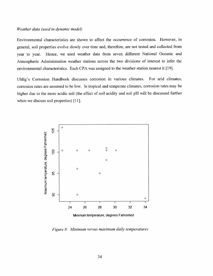
Temperature. We considered both the average daily temperature and temperature index, which
is the ratio of the minimum and maximum daily temperatures and measures temperature
variation. Figure 8 presents a scatter plot of the minimum versus maximum daily temperature.
The scatter plot does not indicate a correlation. However, a simple linear regression of the
maximum daily temperature as a function of the minimum daily temperature yields an R2 value
greater than 0.5, indicating a correlation. Hence, a ratio of the maximum and minimum daily
temperatures was used instead of each factor individually.
We assume that areas with the higher average daily temperatures may have a higher corrosion
occurrence. The more the temperature index decreases, the higher the corrosion occurrence
because of temperature variation.
Total annual precipitation. Precipitation indicates how much water is available for the soil. The
presence of water in the soil increases the likelihood that corrosion will occur. Therefore, we
assume a CPA with more precipitation may have higher corrosion occurrence.
Diameter ofpipe (used in static model)
Wall thickness of the pipe depends on the diameter of the pipe. The thicker the pipe wall is, the
more material there is that needs to corrode before a leak can occur. Hence, it is assumed that
CPAs with higher percentages of pipe with larger diameters may have lower corrosion
occurrence.
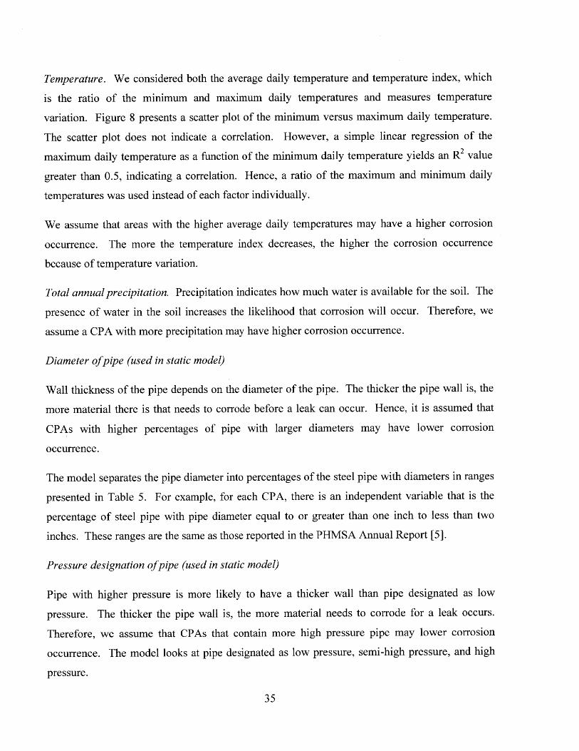
The model separates the pipe diameter into percentages of the steel pipe with diameters in ranges
presented in Table 5. For example, for each CPA, there is an independent variable that is the
percentage of steel pipe with pipe diameter equal to or greater than one inch to less than two
inches. These ranges are the same as those reported in the PHMSA Annual Report [5].
Pressure designation ofpipe (used in static model)
Pipe with higher pressure is more likely to have a thicker wall than pipe designated as low
pressure. The thicker the pipe wall is, the more material needs to corrode for a leak occurs.
Therefore, we assume that CPAs that contain more high pressure pipe may lower corrosion
occurrence. The model looks at pipe designated as low pressure, semi-high pressure, and high
pressure.
35
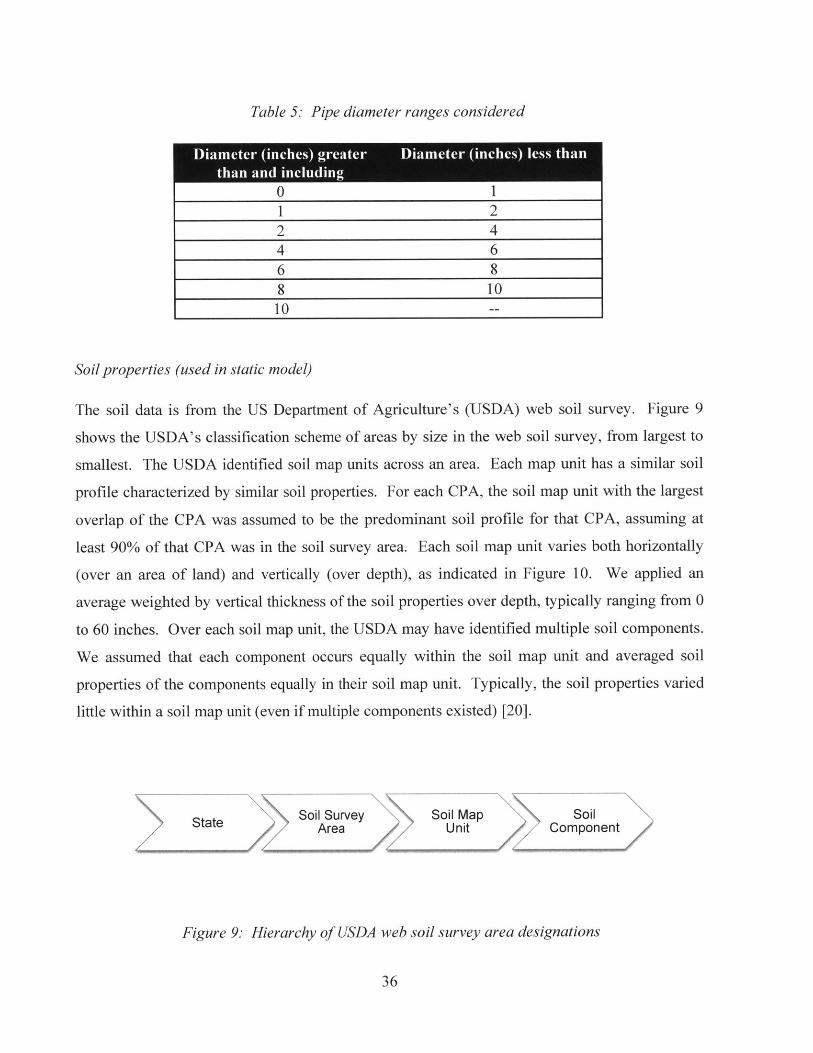
Table 5: Pipe diameter ranges considered
0 11 22) 44 66 88 1010 --
Soil properties (used in static model)
The soil data is from the US Department of Agriculture's (USDA) web soil survey. Figure 9
shows the USDA's classification scheme of areas by size in the web soil survey, from largest to
smallest. The USDA identified soil map units across an area. Each map unit has a similar soil
profile characterized by similar soil properties. For each CPA, the soil map unit with the largest
overlap of the CPA was assumed to be the predominant soil profile for that CPA, assuming at
least 90% of that CPA was in the soil survey area. Each soil map unit varies both horizontally
(over an area of land) and vertically (over depth), as indicated in Figure 10. We applied an
average weighted by vertical thickness of the soil properties over depth, typically ranging from 0
to 60 inches. Over each soil map unit, the USDA may have identified multiple soil components.
We assumed that each component occurs equally within the soil map unit and averaged soil
properties of the components equally in their soil map unit. Typically. the soil properties varied
little within a soil map unit (even if multiple components existed) [20].
State Soil Survey Soil Map SoilArea Unit Component
Figure 9: Hierarchy 0f USDA web soil survey area designations
36
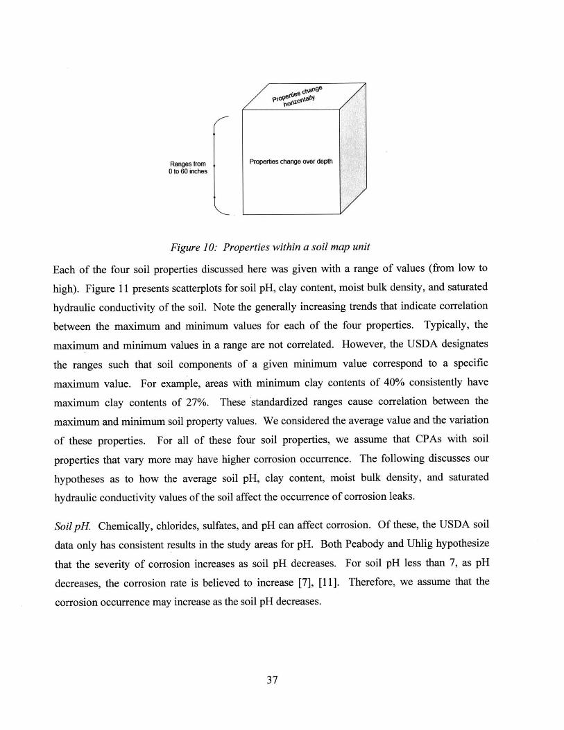
Ranges from Properties change over depth0 to 60 inches
Figure 10: Properties within a soil map unit
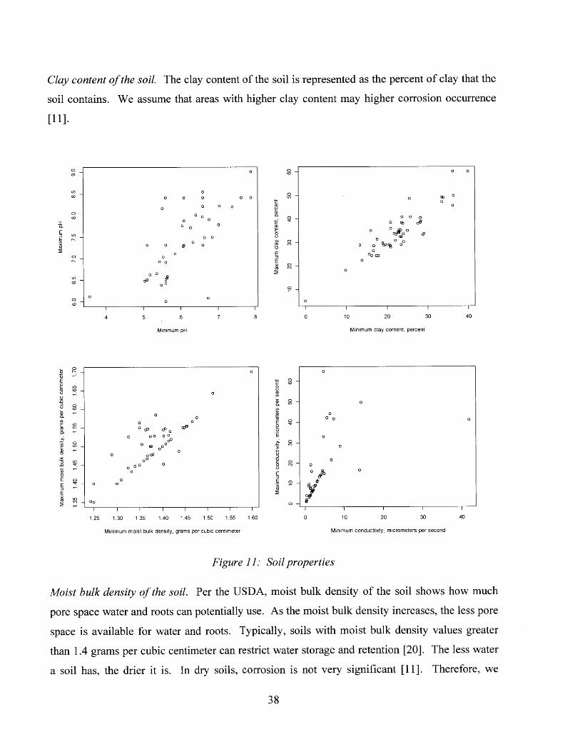
Each of the four soil properties discussed here was given with a range of values (from low to
high). Figure 11 presents scatterplots for soil pH, clay content, moist bulk density, and saturated
hydraulic conductivity of the soil. Note the generally increasing trends that indicate correlation
between the maximum and minimum values for each of the four properties. Typically, the
maximum and minimum values in a range are not correlated. However, the USDA designates
the ranges such that soil components of a given minimum value correspond to a specific
maximum value. For example, areas with minimum clay contents of 40% consistently have
maximum clay contents of 27%. These standardized ranges cause correlation between the
maximum and minimum soil property values. We considered the average value and the variation
of these properties. For all of these four soil properties, we assume that CPAs with soil
properties that vary more may have higher corrosion occurrence. The following discusses our
hypotheses as to how the average soil pH, clay content, moist bulk density, and saturated
hydraulic conductivity values of the soil affect the occurrence of corrosion leaks.
SoilpH Chemically, chlorides, sulfates, and pH can affect corrosion. Of these, the USDA soil
data only has consistent results in the study areas for pH. Both Peabody and Uhlig hypothesize
that the severity of corrosion increases as soil pH decreases. For soil pH less than 7, as pH
decreases, the corrosion rate is believed to increase [7], [11]. Therefore, we assume that the
corrosion occurrence may increase as the soil pH decreases.
37
Clay content of the soil. The clay content of the soil is represented as the percent of clay that the
soil contains. We assume that areas with higher clay content may higher corrosion occurrence
[11].
U?CO
C300
0r-
(C)
C)(D
C:)r-
V)
C)cD
LO
0u')
Ln
C)
LOc')
a)
O3
E
0 a a
00a 0
0 0
0 0
0
1.25~ 1.0 13 .0 1.4 1.a 15 .0
0M
00
000
0 0
4 5 6 7 8
Minimum pH
0 0
00
0 0
o00
000 0 0
00
1.25 1.30 1.35 1.40 1.45 1.50 1.55 1.60
Minimum moist bulk density, grams per cubic centimeter
(0-
0-
0-
00 00 0 o "
o 0c o o
0 00
I I I I
0 1o 20 30 40
Minimum clay content, percent00 0
0
a0 10 20304
I I I I0 10 20 30
Minimum conducthty, micrometers per second
Figure 11: Soil properties
Moist bulk density of the soil. Per the USDA, moist bulk density of the soil shows how much
pore space water and roots can potentially use. As the moist bulk density increases, the less pore
space is available for water and roots. Typically, soils with moist bulk density values greater
than 1.4 grams per cubic centimeter can restrict water storage and retention [20]. The less water
a soil has, the drier it is. In dry soils, corrosion is not very significant [11]. Therefore, we
38
140
0
2
.L5
E
6:
0(0
0Ln
a't
0
assume that as the moist bulk density of the soil decreases (the less water it can potentially store),
the corrosion occurrence may decrease.
Saturated hydraulic conductivity. The saturated hydraulic conductivity measures how easily
water can flow through soil [20]. This measurement is important as the more easily water can
flow through soil, the less likely the occurrence of corrosion is. Less conductive soils can retain
water longer and increase the occurrence of corrosion [11]. Therefore, as the saturated hydraulic
conductivity decreases, we assume that the corrosion occurrence may increase.
Soil resistivity (not included)
The average soil resistivity measurements within a CPA were not used for these analyses despite
frequently being referenced when discussing corrosion rates and the design of cathodic
protection systems. Soil resistivity, typically in ohm-meters or ohm-centimeters, measures how
easily the soil conducts current. As discussed in the literature review, typically, corrosion
occurrence increases as soil resistivity decreases [14]. However, this relationship only holds if
cathodic protection is inadequate [11]. Nevertheless, soil resistivity does affect the design of the
cathodic protection systems (such as the type and number of anodes) and affects how
neighboring current-generating sources such as a different cathodically protected pipeline will
affect the cathodic protection performance. While these data ideally would have been included
in building the models, it was not readily available in an easy to use format.
3.5 Metrics for Measuring Model Performance
Two different types of metrics are considered for measuring the models' performances based on
the results of the cross-validation runs, as indicated in Figure 12. The first set of metrics
measure the predictive ability of the models, or how accurately the models can predict if a leak
will occur or not in a given CPA. The second set of metrics measure how well the models fit the
in-sample data used to build the models. This section describes both sets of metrics.
39

I- - - ____________________________________________ _____________________________________
Figure 12: Schematic of modeling process - cross-validation runs
Measuring pertbrmance of predictive ability
MAPE. As mentioned earlier, the mean average percentage error (MAPE) is the average
difference between the predicted and actual values weighted by the number of predictions [21].
A lower MAPE indicates a better model.
Specificity. Specificity is the percent of predicted "yeses" that are true. For these models, it is
the percent of CPAs that are predicted to have at least one corrosion leak occur that actually had
a corrosion leak occur that year [22]. A higher specificity indicates a better model.
Sensitivity. Sensitivity is the percent of predicted "nos" that are true. For these models, it is the
percent of CPAs that are predicted to have no corrosion leaks occur that actually had no
corrosion leaks that year [22]. A higher sensitivity indicates a better model.
40

Area under the ROC plots. The receiver-operating characteristic (ROC) plots present the
sensitivity and specificity pair for each decision threshold for a binary decision independent
variable. Figure 13 presents an example ROC plot. A model can predict with perfect sensitivity
if the ROC plot passes through the upper left quadrant of the plot. The closer the ROC plot is to
the left vertical axis and the top horizontal axis, the better predictive ability the model has. A
model that has no predictive ability, or does not perform better than guessing, will fall along the
45 degree diagonal from the bottom left corner of the graph to the top right corner of the graph,
indicated by the gray dashed line in Figure 13. The area under the ROC plot indicates the shape
of this plot. The closer the area under the ROC plot is to one, the better the predictive ability of
the model [23].
C?
OP
0CLW)
2
CD
('T03
CD
C?
I I II
0.0 0.2 0.4 0.6
False positive rate
C?0
N-CD(
0D
CO-
0D
W~C3~
0.8 1.0
Figure 13: Example ROC curve
Measuring goodness offit
Residual deviance. The residual deviance measures the amount of unexplained variation in the
model [17]. A lower residual deviance indicates a better model.
AIC. Akaike's information criterion (AIC) penalizes models for using extra parameters [17]. A
lower AIC indicates a better model.
41
'iii
~1

3.5 Summary
We first described why corrosion leaks repaired is used as the measurement of corrosion
occurring in the dependent variable. The cause of a leak is not known until the pipe is excavated
and repaired. We know that corrosion is occurring because of insufficient cathodic protection
but we do not know what is causing this insufficient protection. We examined the predictive
ability of linear, quasi-Poisson, logistic, and random forest regressions. Since logistic
regressions have the smallest error when predicting if a corrosion leak will occur in a CPA or
not, we developed our models using logistic regressions. Two types of data were used: data that
are relatively static over time and data that change over time. Therefore, we developed two
different models using each type of data. The following next chapter analyzes the models using
the data described in this chapter. The hypotheses about the data and the corrosion occurrence
are further examined. Additionally, the metrics discussed for measuring the models'
performances are also discussed in the following chapter.
42
Chapter 4: Results
This chapter discusses the results of the logistic regression models built using both the static and
dynamic data. We examine the significant independent variables to 5% significance for the
various cross-validation runs for the static and dynamic data to see if they match the hypotheses
presented in Section 3.3 and investigate any unusual behavior. We then compare the static and
dynamic logistic regressions with each other, discussing which set of data generally fits the
logistic regressions better and which set of data has better predictive ability.
4.1 Significant Static Independent Variables
The data and results presented here answer the question if corrosion can be predicted in one area
using a model built from another area's performance. Four different USDA defined areas were
used for the static data set. For each cross-validation run, three of the USDA areas were
combined in the in-sample data set and the fourth was used as the out-of-sample data set to test
the predictive ability of the logistic regression built using the in-sample data set. Table 6
presents the significant independent variables found in each of the cross-validation runs using the
static data and describes some characteristics of the log odds ratios estimated in the various
logistic regressions. The coefficient in logistic regressions is the log odds ratio, or the log of the
odds ratio. The odds ratio is the proportion of the number of successes to the number of failures
[17]. Table 6 presents the minimum and the maximum of the log odds ratio, the average value of
the log odds ratio, and the standard deviation of the log odds ratio. The minimum and maximum
values indicate whether the sign of the log odds ratio is consistently negative or positive in each
of the cross-validation runs. The standard deviation of the log odds ratio indicates how much
variation there is between the log odds ratios for the same independent variable in different
cross-validation runs.
The models considered independent variables that are significant to a 5% confidence interval.
Due to the variation of significant independent variables from run to run, the model appears
sensitive to the in-sample data. Especially since the data are from urban areas in close proximity,
this variation of significant independent variables suggest that a model developed using only data
from urban areas. might not accurately represent or predict corrosion leaks for data from rural
areas.
43
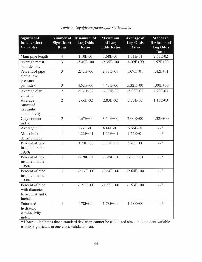
Table 6: Significant fic/ors /br static model
Significant Number of Minimum of Maximum Average of StandardIndependent Significant Log Odds of Log Log Odds Deviation ofVariables Runs Ratio Odds Ratio Ratio Log Odds
RatioMain pipe length 4 1.10E-0I 1.68E-01 1.31E-01 2.63E-02
Average moist 3 -5.40E+00 -2.35E+00 -4.09E+00 1.57E+00bulk densityPercent of pipe 3 2.42E+00 2.73E+01 1.09E+01 1.42E+O1that is lowpressurepH index 3 4.62E+00 6.47E+00 5.32E+00 1.00E+00Average clay 2 -5.3 7E-02 -4.70E-02 -5.03 E-02 4.70E-03contentAverage 2 2.66E-02 2.83E-02 2.75E-02 1.17E-03saturatedhydraulicconductivityClay content 2 1.67E+00 3.54E+00 2.60E+00 1.32E+00indexAverage pH 1 6.66E-01 6.66E-0I 6.66E-0l -- *
Moist bulk 1 1.22E+01 1.22E+01 1.22E+01 -- *
density indexPercent of pipe 1 3.70E+00 3.70E+00 3.70E+00 - *installed in the1930sPercent of pipe I -7.28E-01 -7.28E-01 -7.28E-01 -- *
installed in the1960sPercent of pipe 1 -2.64E+00 -2.64E+00 -2.64E+00 - *installed in the1990sPercent of pipe 1 -1.53E+00 -1.53E+00 -1.53E+O -- *
with diameterbetween 4 and 6inchesSaturated 1 1.78E+00 1.78E+00 1.78E+00 -- *
hydraulicconductivityindex* Note: -- indicates that a standard deviation cannot be calculated since independent variableis only significant in one cross-validation run.
44

The length of steel main pipe is consistently significant in all four runs. The log odds ratios are
positive and are consistent with our hypothesis that as the length of the steel main pipe increases
in a CPA, the likelihood of corrosion occurrence increases. It is not surprising that the length of
steel main pipe in the CPA is consistently significant since it may be an indication of the
complexity of the CPA.
The average moist bulk density is significant in three of the cross-validation runs and the moist
bulk density index is significant in the fourth cross-validation run. The log odds ratios for the
average moist bulk density are consistently positive, which supports our hypothesis. The moist
bulk density index has a positive log odds ratio indicating that as variation in moist bulk density
values increase within the CPA, the likelihood of corrosion occurrence also increases. This is
consistent with our hypothesis presented in Section 3.3.
The percent of main pipe designated as low pressure is significant in three out of the four cross-
validation runs. The log odds ratios are consistently positive but vary from 2.4 to 27.3. 27.3 is
an outlier; it is an order of magnitude greater than the log odds ratios for the other instances that
the percentage of low pressure pipe is significant. Furthermore, it is at least an order of
magnitude greater than the log odds ratios of the other independent variables. Figure 14 presents
the distribution of the percentage of steel main pipe in a CPA that is designated at each pressure
in each of the in-sample data sets. The horizontal axis gives the percentage of pipe that is
designated as low pressure, semi-high pressure, or high pressure within a CPA. The vertical axis
gives the number of CPAs that have a similar percentage of pipes with the same pressure type.
For example, most of the CPAs have no pipe designated as low or semi-high pressure as
indicated by the high count of CPAs at the left side of the graphs. The histograms indicate
similar distribution for each cross-validation set with the low percentages of low pressure and
semi-high pressure pipe.
Figure 15 presents the scatter plots of the leak occurrence within a given CPA versus the
percentage of pipe by each pressure designation. The horizontal axis gives the percentage of
pipe that is designated as low pressure, semi-high pressure, or high pressure within a CPA. The
vertical axis indicates if a corrosion leak has occurred in the CPA (0 if no corrosion leaks
occurred and 1 if at least one corrosion leak occurred). Again, the scatter plots are similar for
each cross-validation run. The only difference is that Run 2 does not have any CPAs with a high
45
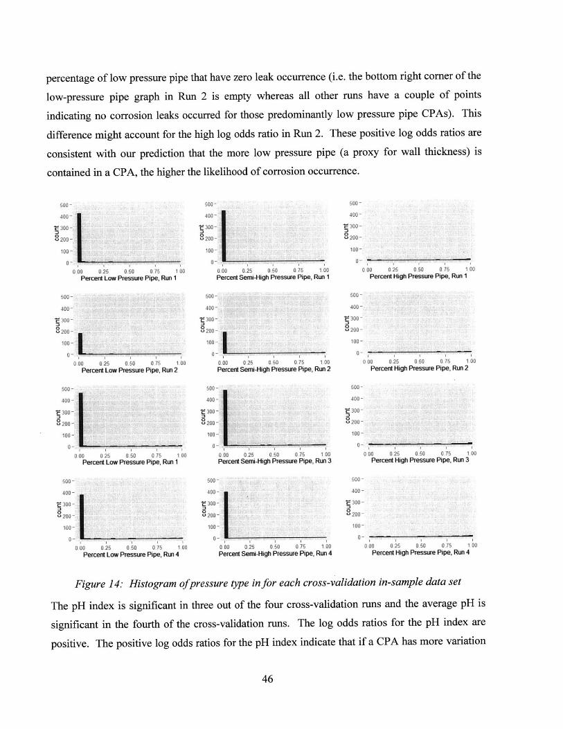
percentage of low pressure pipe that have zero leak occurrence (i.e. the bottom right corner of the
low-pressure pipe graph in Run 2 is empty whereas all other runs have a couple of points
indicating no corrosion leaks occurred for those predominantly low pressure pipe CPAs). This
difference might account for the high log odds ratio in Run 2. These positive log odds ratios are
consistent with our prediction that the more low pressure pipe (a proxy for wall thickness) is
contained in a CPA, the higher the likelihood of corrosion occurrence.
:30 I
Percent Low Pressure Pipe, Run 1
-4 LI
:30:3
0
0
Percent Semi-High Pressure Pipe, Run 1
c:30
Percent High Pressure Pipe, Run 1
:30
IPercent Low Pressure Pipe, Run 2
0
Percent Low Pressure Pipe, Run 1
Percent Low Pressure Pipe, Run 4
Percent Semi-High Pressure Pipe, Run 2
Percent Semi-High Pressure Pipe, Run 3
Percent Semi-High Pressure Pipe, Run 4
Percent High Pressure Pipe, Run 2
I:3
Percent High Pressure Pipe, Run 3
I:30
Percent High Pressure Pipe, Run 4
Figure 14: Histogram ofpressure type in for each cross-validation in-sample data set
The pH index is significant in three out of the four cross-validation runs and the average pH is
significant in the fourth of the cross-validation runs. The log odds ratios for the pH index are
positive. The positive log odds ratios for the pH index indicate that if a CPA has more variation
46
I:30 I
I
_'I

in soil pH values, the more likely corrosion is to occur. This is consistent with the hypothesis
proposed in Section 3.3. The log odds ratio for the average pH is positive in Run 3. This
positive log odds ratio is inconsistent with the hypothesis proposed in Section 3.3 that states that
the more acidic the soil pH is, the more likely corrosion is to occur.
ea.. *00 o* 400 ** * 0 *(U
41)
CU)
Ij
T~
C0,
C:
4)
(U
T
C
C)
2
0~
a)
C)
C
C)
4)
T-
-Y 4
0M
C
UT
Percent Semi-High Pressure Pipe, Run 1
Percent Semi-High Pressure Pipe, Run 2
Percent Semi-High Pressure Pipe, Run 3
Percent Low Pressure Pipe, Run 1
Percent Low Pressure Pipe, Run 2
Percent Low Pressure Pipe, Run 3
Percent Low Pressure Pipe, Run 4
0CC)
C)
)
a).
C)
0D
CU
C)
Percent High Pressure Pipe, Run 1
Percent High Pressure Pipe, Run 2
+.+ . . + + . + **
Percent High Pressure Pipe, Run 3
Percent High Pressure Pipe, Run 4
Figure 15: Histogram ofpressure type in for each cross-validation in-sample data set
The average clay content is significant in two out of the four cross-validation runs. The clay
content index is significant in the other two cross-validation runs. The log odds ratios for the
average clay content are negative, which indicates that the amount of clay content and the
corrosion occurrence are inversely related and contradict the hypothesis presented in Section 3.3.
The log odds ratios for the clay content index are positive and consistent with our hypothesis that
the more variation in clay content, the more likely that corrosion is to occur.
47
Percent Semi-High Pressure Pipe, Run 4

The average saturated hydraulic conductivity is only significant in two of the four cross-
validation runs while the saturated hydraulic conductivity index is significant in one of the four
cross-validation runs. The log odds ratios for the average saturated hydraulic conductivity are
positive indicating that a higher saturated hydraulic conductivity means more corrosion. This
contradicts our hypothesis that lower saturated hydraulic conductivity indicates higher corrosion
occurrence. The log odds ratio for the saturated hydraulic conductivity is positive indicating that
more variation in the saturated hydraulic conductivity within the CPA increases the likelihood of
corrosion occurrence.
The percent of pipe installed in the 1930s, the percent of pipe installed in the 1960s, and the
percent of pipe installed in the 1990s are each significant in one of the four cross-validation runs.
The log odds ratio for the 1930s pipe is positive, which indicates that more pipe installed in the
1930s increases the occurrence of corrosion. The log odds ratios for the 1960s and 1990s pipe
are negative. This is consistent with Kiefner and Trench's observations, mentioned in the
literature review, that corrosion occurrence is higher for pipe installed in decades before the
1960s that had poorer corrosion practices during construction [10].
The percent of pipe that is between 4 and 6 inch diameter is significant in one out of the three
cross-validation runs. Its log odds ratio is negative. The negative log odds ratio is consistent
with our hypothesis that pipe with larger diameters have a decreased likelihood of corrosion
occurrence.
We are surprised that the percent of steel main pipe installed in the various decades is not more
frequently considered significant since the installation decade not only indicates common
corrosion practices but also the age of the pipe and its corrosion control systems. One expects
that pipe installed in the same decade are installed with similar installation practices (e.g.
coatings, pipe manufacturing practices). Perhaps since pipe installed in similar decades have
similar installation methods, other factors such as the neighborhood, the size of the pipe, or the
pressure designation represent the installation practices.
Each of the soil properties consistently influences the likelihood of corrosion occurrence.
However, it is inconsistent between each cross-validation run if the average value of the soil
property or the variation of the soil property within the CPA is what influences the corrosion
48

occurrence. For the moist bulk density and saturated hydraulic conductivity, the average value
has a greater influence. For the soil pH, variation has a greater influence on corrosion
occurrence. Further investigation is recommended to see if expanding the data set causes more
consistency in whether the average value of the soil property or the variation of the soil property
has a greater influence on corrosion occurrence. Additionally, the soil pH, clay content, and
average hydraulic conductivity values have log odds ratios that do not support the hypotheses
discussed in Section 3.3.
4.2 Significant Dynamic Independent Variables
The data and results presented in this section answer the question if data from one year can be
used to predict where corrosion is most likely to occur in the next year. The dynamic model uses
data from Area A in Year X to predict the number of corrosion leaks that will occur in Area B
during Year X+1. Data from two urban areas were used for the logistic regression models.
Table 7 presents the significant independent variables found in each of the cross-validation runs
for the dynamic data set and describes some characteristics of the coefficient estimate in the
model. Unlike the static data, no independent variable is significant for all of the in-sample data
sets used to build the logistic regression model, indicating variation in the data set. Since this
data set only presented information from urban areas, it is unclear if the model would apply well
to data from suburban and rural areas.
The length of the steel main pipe within a CPA is significant in three of the four cross-validation
runs. The one cross-validation run in which the length of the steel main pipe within the CPA is
not significant, the number of steel services within a CPA is significant. Both the length of the
steel main pipe and the number of steel services have positive log odds coefficients, indicating
that the more steel there is within a CPA, the more likely corrosion leaks will occur. This
matches our hypotheses regarding corrosion occurrence and amount of steel contained within a
CPA in Section 3.3 and is consistent with the results of the static model.
49
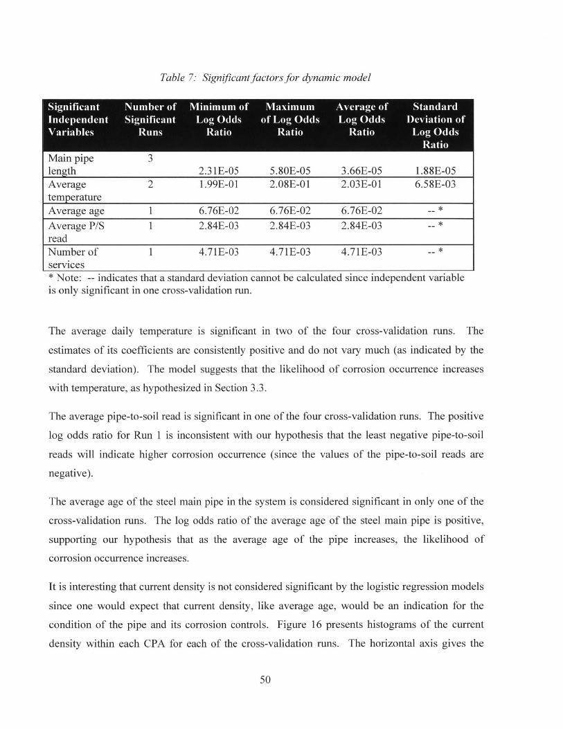
Table 7: Signficantuactors for dynamic model
Significant Number of Minimum of Maximum Average of StandardIndependent Significant Log Odds of Log Odds Log Odds Deviation ofVariables Runs Ratio Ratio Ratio Log Odds
RatioMain pipe3length 2.3 1E-05 5.80E-05 3.66E-05 1.88E-05Average 2 1.99E-01 2.08E-01 2.03E-01 6.58E-03temperatureAverage age 1 6.76E-02 6.76E-02 6.76E-02 -- *
Average P/S 1 2.84E-03 2. 84E-03 2.84E-03 -- *readNumber of 1 4.71E-03 4.71E-03 4.71E-03 -- *services* Note: -- indicates that a standard deviation cannot be calculated since independent variableis only significant in one cross-validation run.
The average daily temperature is significant in two of the four cross-validation runs. The
estimates of its coefficients are consistently positive and do not vary much (as indicated by the
standard deviation). The model suggests that the likelihood of corrosion occurrence increases
with temperature, as hypothesized in Section 3.3.
The average pipe-to-soil read is significant in one of the four cross-validation runs. The positive
log odds ratio for Run 1 is inconsistent with our hypothesis that the least negative pipe-to-soil
reads will indicate higher corrosion occurrence (since the values of the pipe-to-soil reads are
negative).
The average age of the steel main pipe in the system is considered significant in only one of the
cross-validation runs. The log odds ratio of the average age of the steel main pipe is positive,
supporting our hypothesis that as the average age of the pipe increases, the likelihood of
corrosion occurrence increases.
It is interesting that current density is not considered significant by the logistic regression models
since one would expect that current density, like average age, would be an indication for the
condition of the pipe and its corrosion controls. Figure 16 presents histograms of the current
density within each CPA for each of the cross-validation runs. The horizontal axis gives the
50
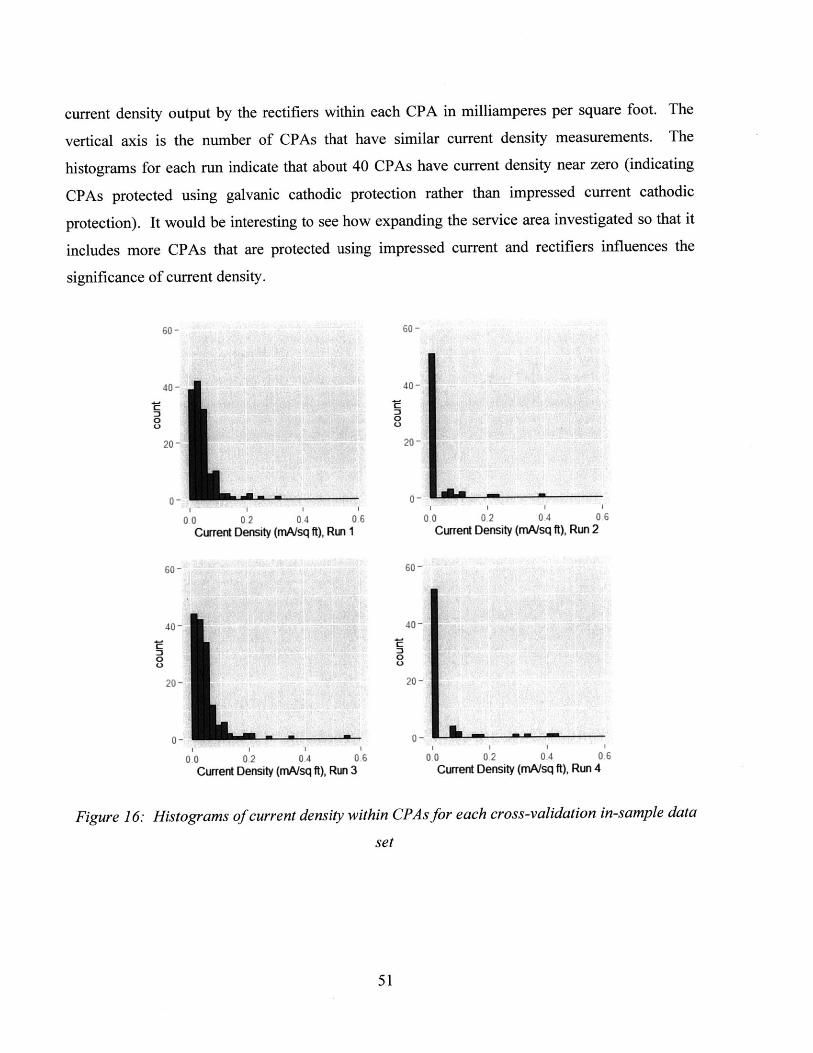
current density output by the rectifiers within each CPA in milliamperes per square foot. The
vertical axis is the number of CPAs that have similar current density measurements. The
histograms for each run indicate that about 40 CPAs have current density near zero (indicating
CPAs protected using galvanic cathodic protection rather than impressed current cathodic
protection). It would be interesting to see how expanding the service area investigated so that it
includes more CPAs that are protected using impressed current and rectifiers influences the
significance of current density.
60 -
0 0C)
Go -
Current Density (mA/sq ft), Run 1
60-
:30L)0
C)
Current Density (nA/sq ft), Run 3
Current Density (nA/sq ft), Run 2
60-
Current Density (mA/sq ft), Run 4
Figure 16: Histograms of current density within CPAs for each cross-validation in-sample data
set
51

4.3 Comparing the Two Models
To compare the models built using the static data against the dynamic data, we examined both
how the in-sample data performed (how well does the in-sample data fit the logistic regression)
and how the out-of-sample data performed (how well does the logistic regression predict
corrosion leaks using the out-of-sample data). We evaluated the fit of the logistic regressions
using the residual deviance and Akaike's information criterion (AIC). The residual deviance
measures the amount of unexplained variation in the model while the AIC penalizes models for
using extra parameters. For both the residual deviance and AIC, smaller values indicate that one
model fits the data better than another [17]. Table 8 presents information regarding the fit of the
data in the various cross-validation runs to the corresponding logistic regressions. The residual
deviance and the AIC are generally larger for the static model than the dynamic model.
Run 1
0.0 0.2 04 0.6 0.8 1.0
False positive rate
Run 3
CD
C)
(.4inC:,
C")C)
C'4
C)
MCDC)
2
2
Run 2
00 0.2 0.4 0.6 08 10
False positive rate
Run 4
_jF
0.0 0.2 04 0.6 08 10 0.0 0.2 0.4 0.6 0 8
False positive rate False positive rate
Figure 17: ROC curves for the static model
I52
C)
CO
M
C"C)
(Dr-
(DC)
C)
C
q -
CO -C)
LP -Ol
C)
C'46
C?C)
WCD
C)
C)
C'
C
10
CD
CDC)
W -CD
C:)
C)
P -C)
a)C.
C'
C)
n
C)
CD
(DC)
WC)
C>
C146
C)C.
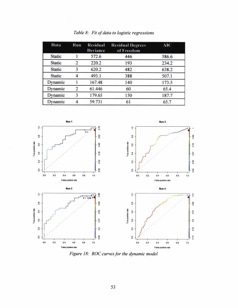
Table 8: Fit of data to logistic regressions
Static 1 572.6 446 586.6Static 2 220.2 193 234.2Static 3 620.2 482 638.2Static 4 493.1 388 507.1
Dynamic 1 167.48 140 173.5Dynamic 2 61.446 60 65.4Dynamic 3 179.65 150 187.7Dynamic 4 59.731 61 65.7
Run I
0.0 0.2 0.4 0.6 0.8 1.0
False positive rate
Run 3
0.1 0 08 0
0
2
a
2
-~ 0
Run 2
0.0 0.2 04 0.6 08 1,0
False positive rate
Run 4
0.0 0.2 0.4 0.6 0.8 1,0 00 0.2 0.4 06
False positive rate False positive rate
Figure 18: ROC curves for the dynamic model
53
I
a)
2
in C
2)
0.8 1.0
C4
C)
Q
CNC)
COC)M
(DCD
UDC)
C4Ci
9C)
C.
C.')
C,
C)
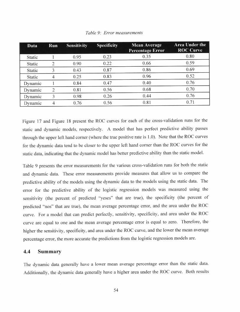
Table 9: Error measurements
Static 1 0.95 0.23 0.35 0.80
Static 2 0.90 0.22 0.66 0.59
Static 3 0.43 0.87 0.86 0.69
Static 4 0.25 0.83 0.96 0.52
Dynamic 1 0.84 0.47 0.40 0.76
Dynamic 2 0.81 0.56 0.68 0.70
Dynamic 0.98 0.26 0.44 0.76
Dynamic 4 0.76 0.56 0.81 0.71
Figure 17 and Figure 18 present the ROC curves for each of the cross-validation runs for the
static and dynamic models, respectively. A model that has perfect predictive ability passes
through the upper left hand corner (where the true positive rate is 1.0). Note that the ROC curves
for the dynamic data tend to be closer to the upper left hand corner than the ROC curves for the
static data, indicating that the dynamic model has better predictive ability than the static model.
Table 9 presents the error measurements for the various cross-validation runs for both the static
and dynamic data. These error measurements provide measures that allow us to compare the
predictive ability of the models using the dynamic data to the models using the static data. The
error for the predictive ability of the logistic regression models was measured using the
sensitivity (the percent of predicted "yeses" that are true), the specificity (the percent of
predicted "nos" that are true), the mean average percentage error, and the area under the ROC
curve. For a model that can predict perfectly, sensitivity, specificity, and area under the ROC
curve are equal to one and the mean average percentage error is equal to zero. Therefore, the
higher the sensitivity, specificity, and area under the ROC curve, and the lower the mean average
percentage error, the more accurate the predictions from the logistic regression models are.
4.4 Summary
The dynamic data generally have a lower mean average percentage error than the static data.
Additionally, the dynamic data generally have a higher area under the ROC curve. Both results
54
indicate that the dynamic models are better at predicting if a leak will occur than the static
models.
Since the soil data are consistently significant in the static models but are neither specific to the
CPAs nor recently obtained, it is possible that using new soil property measurements specific to
the CPAs of interest will yield better predictive ability. The sensitivity for the dynamic data are
generally higher than the sensitivity for the static data indicating that the dynamic data are better
for predicting when corrosion leaks are more likely to occur. Conversely, the specificity for the
static data is better than that of the dynamic data. However, for both the dynamic and static data,
the sensitivity tends to be higher than the specificity. This means that both models tend to be
better at predicting where leaks will occur rather than where leaks will not occur.
55

Chapter 5: Conclusions
5.1 Summary of Results
The occurrence of structural failures due to corrosion is increasing throughout the country as
infrastructure installed a half-century or more ago continues to age. There is increased attention
towards evaluating current corrosion control practices and identifying and repairing leaks due to
corrosion on natural gas pipe. Part of this effort involves identifying areas at greater risk from
corrosion in order to better optimize resources and appropriately monitor these areas. Most
common methods for identifying at risk areas involve retroactively examining pipe that have
large concentration of leaks due to corrosion. This thesis investigates if at corrosion-prone areas
can be identified using various operational, environmental, and historical factors.
We found that logistic regressions that model if a corrosion leak will occur in a given CPA result
in more accurate predictions than linear, quasi-Poisson, and random forest regressions. We
examined two different types of data available: data that changed each year (the dynamic data)
and data that did not change each year (the static data). The logistic regression models built with
the dynamic data generally predicted corrosion leaks better than the logistic regression models
built with the static data.
The length of steel main pipe within a CPA, the percentage of steel main pipe designated as low
pressure, the average moist bulk density, the average clay content, the average saturated
hydraulic conductivity, and the variation in soil pH were typically significant for the logistic
regressions using the static data. The average soil pH, average moist bulk density, and the
average saturated hydraulic conductivity did not influence corrosion occurrence as we expected.
The length of steel main pipe within a CPA and the average temperature were typically
significant for the logistic regressions for the dynamic data. The current density outputted by the
rectifiers did not influence corrosion occurrence as we expected.
The residual deviance and AIC have generally smaller values for the dynamic data than the static
data, indicating that the dynamic data fit a logistic regression better than the static data.
Additionally, the dynamic model predicts if corrosion will occur more accurately than the static
model. The mean average percentage error is generally lower for the dynamic model than the
56
static model and the area under the ROC curve is generally greater for the dynamic model than
the static model. For both the static and the dynamic models, the sensitivity tends to be higher
than the specificity indicating that the models are better at predicting where corrosion is more
likely to occur than where it is more likely to not occur.
5.2 Recommendations for Future Work
Recommendations for future work are as follows:
- The models developed in this thesis only looked at data in a small part of PG&E's
network (16.8% of the steel distribution main pipe for the static models and 9.6% for the
dynamic models) that is located in predominantly urban areas. Future work can be done
to incorporate data from across PG&E's entire gas distribution network (including both
urban, suburban, and rural areas). Of particular interest is if greater variation in soil data
or local maintenance practices would provide information on some areas having higher
leak occurrence than others within PG&E.
- Similarly, this model only considers the steel pipe in PG&E's system (about half of
PG&E's distribution network) and only accounts for leaks due to corrosion. Future work
can update model to predict all leak threats as identified by PHMSA for both steel and
plastic pipe. PG&E can use the results from more inclusive predictive models to
proactively manage leaks.
- These models should be updated by using more current and site-specific soil data and
weather data. Specifically, we recommend using soil resistivity data within the CPAs of
interest. Additionally, since weather data from only 7 NOAA weather stations were used
(with an average 284 miles of steel distribution pipe between each weather station), it
would be interesting to see if more granularity in the weather data influences the results
of the predictive models.
* Finally, we recommend that PG&E consider updating the models to include the effects of
stray current corrosion due to neighboring pipe's cathodic protection systems and the rail
systems. Stray current is current that originates outside of the pipeline's cathodic
protection system. Examples of stray current sources include another pipeline's
57

impressed current cathodic protection system or from the direct current powering a
nearby rail transit system. The interference of these additional current sources can cause
corrosion on the pipeline [7]. Including stray current in the models may provide further
guidance as to why some areas are more prone to corrosion than other areas.
58
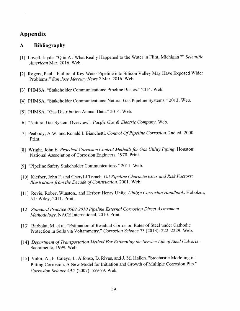
Appendix
A Bibliography
[1] Lovell, Jayde. "Q & A: What Really Happened to the Water in Flint, Michigan ?" ScientificAmerican Mar. 2016. Web.
[2] Rogers, Paul. "Failure of Key Water Pipeline into Silicon Valley May Have Exposed WiderProblems." San Jose Mercury News 2 Mar. 2016. Web.
[3] PHMSA. "Stakeholder Communications: Pipeline Basics." 2014. Web.
[4] PHMSA. "Stakeholder Communications: Natural Gas Pipeline Systems." 2013. Web.
[5] PHMSA. "Gas Distribution Annual Data." 2014. Web.
[6] "Natural Gas System Overview". Pacific Gas & Electric Company. Web.
[7] Peabody, A W, and Ronald L Bianchetti. Control OfPipeline Corrosion. 2nd ed. 2000.Print.
[8] Wright, John E. Practical Corrosion Control Methods for Gas Utility Piping. Houston:National Association of Corrosion Engineers, 1970. Print.
[9] "Pipeline Safety Stakeholder Communications." 2011. Web.
[10] Kiefner, John F, and Cheryl J Trench. Oil Pipeline Characteristics and Risk Factors:Illustrations from the Decade of Construction. 2001. Web.
[11] Revie, Robert Winston., and Herbert Henry Uhlig. Uhlig's Corrosion Handbook. Hoboken,NJ: Wiley, 2011. Print.
[12] Standard Practice 0502-2010 Pipeline External Corrosion Direct AssessmentMethodology. NACE International, 2010. Print.
[13] Barbalat, M. et al. "Estimation of Residual Corrosion Rates of Steel under CathodicProtection in Soils via Voltammetry." Corrosion Science 73 (2013): 222-2229. Web.
[14] Department of Transportation Method For Estimating the Service Life of Steel Culverts.Sacramento, 1999. Web.
[15] Valor, A., F. Caleyo, L. Alfonso, D. Rivas, and J. M. Hallen. "Stochastic Modeling of
Pitting Corrosion: A New Model for Initiation and Growth of Multiple Corrosion Pits."
Corrosion Science 49.2 (2007): 559-79. Web.
59
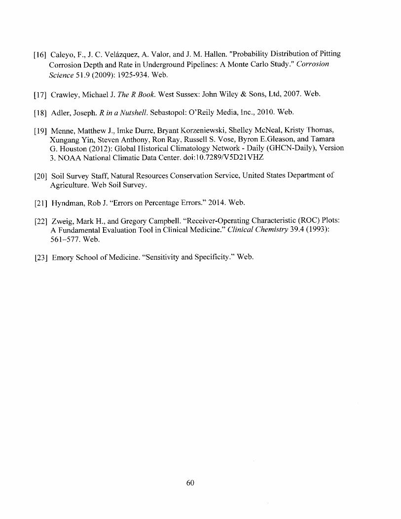
[16] Caleyo, F., J. C. Velazquez, A. Valor, and J. M. Hallen. "Probability Distribution of Pitting
Corrosion Depth and Rate in Underground Pipelines: A Monte Carlo Study." Corrosion
Science 51.9 (2009): 1925-934. Web.
[17] Crawley, Michael J. The R Book. West Sussex: John Wiley & Sons, Ltd, 2007. Web.
[18] Adler, Joseph. R in a Nutshell. Sebastopol: O'Reily Media, Inc., 2010. Web.
[19] Menne, Matthew J., Imke Durre, Bryant Korzeniewski, Shelley McNeal, Kristy Thomas,Xungang Yin, Steven Anthony, Ron Ray, Russell S. Vose, Byron E.Gleason, and TamaraG. Houston (2012): Global Historical Climatology Network - Daily (GHCN-Daily), Version3. NOAA National Climatic Data Center. doi:10.7289/V5D21VHZ
[20] Soil Survey Staff, Natural Resources Conservation Service, United States Department ofAgriculture. Web Soil Survey.
[21] Hyndman, Rob J. "Errors on Percentage Errors." 2014. Web.
[22] Zweig, Mark H., and Gregory Campbell. "Receiver-Operating Characteristic (ROC) Plots:A Fundamental Evaluation Tool in Clinical Medicine." Clinical Chemistry 39.4 (1993):561-577. Web.
[23] Emory School of Medicine. "Sensitivity and Specificity." Web.
60

B Commonly Used Abbreviations
AIC: Akaike's information criterion
CPA: cathodic protection area
ECDA: external corrosion direct assessment
MAPE: mean average percentage error
P/S read: pipe-to-soil read
PHMSA: Pipeline and Hazardous Materials Safety Administration
ROC: receiver-operating characteristic
USDA: United States Department of Agriculture
61