lable at ScienceDirect

Ocean & Coastal Management 130 (2016) 317e327

Contents lists avai

Ocean & Coastal Management

journal homepage: www.elsevier .com/locate/ocecoaman

Predicting common bottlenose dolphin habitat preference todynamically adapt management measures from a Marine SpatialPlanning perspective

G. La Manna a, b, *, F. Ronchetti a, b, G. Sar�a c, a

a MareTerra Onlus - Environmental Research and Conservation, Regione Salondra 9, 07041 Alghero, Italyb CTS, Dipartimento Conservazione Della Natura, Via Albalonga 3, 00161 Roma, Italyc Dipartimento di Scienze Della Terra e Del Mare, Via Delle Scienze ed. 16, Universit�a Degli Studi di Palermo, Palermo, Italy

a r t i c l e i n f o

Article history:Received 16 December 2015Received in revised form11 July 2016Accepted 14 July 2016

Keywords:Tursiops truncatusSpatial distributionMaxEntMediterranean SeaMarine Spatial Planning

* Corresponding author. MareTerra Onlus - Enviroservation, Regione Salondra 9, 07041 Alghero, Italy.

E-mail addresses: gabriella.lamanna@gmail.com (Ggmail.com (F. Ronchetti), gsara.unipa@gmail.com (G.

http://dx.doi.org/10.1016/j.ocecoaman.2016.07.0040964-5691/© 2016 Elsevier Ltd. All rights reserved.

a b s t r a c t

At the European Level, SACs (Special Areas of Conservation) are considered among the most reliable toolsfor increasing the efficiency of protective actions and to identify species vulnerability hotspots acrossspatial scales. Nevertheless, SACs may fail in their scope when design and management are notdynamically adapted to meet ecological principles. Knowledge of the spatial distribution of relevant keyspecies, such as common bottlenose dolphin (Tursiops truncatus), is crucial in order to achieve theobjective of the Habitat Directive (92/43/EEC), and is a fundamental step in the process of Marine SpatialPlanning. From this perspective, new data and analysis are required to produce forecasts at spatio-temporal scales relevant to individual organisms. Here, we propose a study based on a MaxEntmodelling exercise to define the spatial distributional patterns of bottlenose dolphin at different tem-poral scales (over periods of multiple months and years) to increase the ecological understanding of howthe species use the eco-space, and to delimit boundaries of a SAC in the waters surrounding LampedusaIsland, a hotspot for cetaceans in the Southern Mediterranean Sea. We show that bottlenose dolphinprefer shallower feeding grounds that often host complex and rich food webs, but also that this pref-erence is constrained by disturbance factors such as boat traffic. As sea-related tourism, includingdolphin-watching, is one of the most important economic activities of the island, the study results can beused from a management perspective, in order to reach a solution regarding two apparently conflictingneeds - species protection and economic development.

© 2016 Elsevier Ltd. All rights reserved.

1. Introduction

Global environmental change is forcing organisms to acclimate,adapt and/or migrate to track alterations in their environmentacross space and time, and there is a need to improve projections ofthe future status of marine biodiversity under rapidly changingconditions (Pacifici et al., 2015). Large ecosystem shifts are, how-ever, ultimately driven by cumulative impacts of small-scale pro-cesses acting at organismal and population levels. In order topredict future changes in species distributions, new data arerequired to produce forecasts at spatio-temporal scales relevant to

nmental Research and Con-

. La Manna), ronchetti.fabio@Sar�a).

individual organisms (Halpern et al., 2015).Cetaceans are among themost threatenedmarine species. These

threats have become such a concern as to warrant a specific regu-latory action at the European Community level, as dictated by theHabitats Directive (Council Directive 92/43/EEC on the Conserva-tion of natural habitats and of wild fauna and flora). This Directiveaims to establish a network of SACs (Special Areas of Conservation)that are known collectively as “Natura 2000”. The Natura networkcomprises sites identified by the Member States as hosting partic-ular habitat types (listed in Annex I of the Directive), or the habitatsof particular species (listed in Annex II). To date, two species ofcetaceans have been listed on Annex II, namely the harbour por-poise (Phocoena phocoena) and the common bottlenose dolphin(Tursiops truncatus, Montagu, 1821). SACs, and other Marine Pro-tected Area in general, are considered among themost reliable toolsfor increasing the efficiency of conservation actions and for

G. La Manna et al. / Ocean & Coastal Management 130 (2016) 317e327318

defining species vulnerability hotspots across spatial scales (Canadaet al., 2005; Agardy et al., 2011).

Knowing the distribution and ranging patterns of cetaceans isimportant for adapting effective boundaries for SACs and MPAs andis a fundamental requirement for all species listed in the HabitatsDirective. Moreover, knowing the spatial distribution of ecologi-cally relevant species is also one of the fundamental steps inachieving the goals of most Marine Spatial Planning Directivesworldwide (e.g., the European Directive 2014/89 “Establishing aframework for maritime spatial planning”, or the “Interim Frame-work for Effective Coastal andMarine Spatial Planning” in the USA).In fact, among basic principles proposed to address Ecosystem-based Marine Spatial Planning, those dealing with key species,such as Tursiops truncatus, are essential in increasing the reliabilityof management measures (sensu Stamoulis and Delevaux, 2015).Dolphins are at the top of trophic chains worldwide and they sharethe role of ecosystem functioning drivers with a few other top levelspecies. An anomalous fluctuation in their distributional range dueto the pervasive effects of human actions can alter communitystructure and depress ecosystem functioning.

However, for most marine species (such as cetaceans and fish),identifying marine areas useful to their life and reproduction maybe difficult. The high mobility of many marine species and thedifficulty in observing them may complicate the investigation oftheir distribution considerably, increasing research costs andexperimentation time. An effective ecosystem-level managementdepends acutely upon the quality of information available, not onlyfor defining boundaries but also for understanding how these areasare used by animals, and which components (biotic, abiotic andfactors of anthropogenic origin) influence their distribution andabundance (Wilson et al., 1997). Marine mammals are recognizedas not permanently resident species (Wilson et al., 1997), and thismakes the design of SACs/MPAs and the related management ac-tions highly challenging. Even if many cetaceans have been shownto display relatively consistent preferences in terms of environ-mental variables and bottom topography (Hastie et al., 2005), fewstudies have predicted the habitat use of bottlenose dolphins inrelation to environmental variables through the application ofspecies distribution modelling (SDMs) in the Mediterranean Sea(Canadas et al., 2002, 2005; Azzellino et al., 2008, 2012; Gomezet al., 2008; Marini et al., 2014). SDMs have a long tradition inecology to help both researchers and managers to increase theirunderstanding of current species distribution patterns, and topredict future distributions in the face of climate change, human-assisted invasions, and many other ongoing environmentalchanges (Yackulic et al., 2013). One of the most recently used SDMsis that based on the Maximum Entropy (MaxEnt) method. MaxEntis a presence-only statistical model, and it is highly reliable inproducing useful predictions when absence data are not availableor not sufficiently reliable. In the case of cetacean sampling, manylocations cannot be surveyed systematically or may receive littlesurvey effort, leading to a lack of definitive absence data. MaxEntrepresents the most effective correlative modelling approach incontext of SDM (Guisan and Thuiller, 2005), providing an importantecological tool for the prediction of species geographical distribu-tion within the context of environmental change from local toglobal. MaxEnt attempts to minimize the relative entropy betweentwo probability densities, one estimated from occurrence data andthe other from the background environment defined in covariatespace (Elith et al., 2011). The maximum entropy distribution is builtonly from what is known about the occurrence of the species andits associated variables, while avoiding making assumptions aboutanything unknown (Jaynes, 1989). This method is especially usefulfor modelling species distributions with incomplete information onsampling effort and not independent data, and is becoming an

increasingly important tool in the field of marine conservation andmanagement (Edren et al., 2010; Thorne et al., 2012). Moreover,MaxEnt has a predictive power that is consistently competitivewith the highest performing methods (Elith et al., 2006, 2011).Here, we used MaxEnt to define the spatial distribution pattern ofT. truncatus, at different temporal scales (years and months) in or-der to increase the ecological knowledge about the species, and todefine boundaries of a SAC in the waters surrounding the Archi-pelago of Pelagie (Southern Mediterranean Sea). Such an area is akey habitat for cetaceans (Ben Naceur et al., 2004; Canese et al.,2006) and meets all the criteria required for the localization ofSACs: i) the continuous or regular presence of the species, asdemonstrated in the past and in the present study on the basis ofMaxEnt predictions; ii) good population density, in relation toneighbouring areas (Pulcini et al., 2010); iii) high ratio of juvenilesto adults all year round (Pace et al., 2003).

2. Methods

2.1. Study area

Lampedusa is the biggest island in the Archipelago of Pelagie(Southern Mediterranean Sea), with an extension of 20 km2 and alength of 10.5 km. It is located on the northern African continentalshelf, about 130 km from the Tunisian coast and 205 km from theSicilian coast. This region is an exchange area for the water massesof the eastern and western Mediterranean basins, with a complexbathymetry that strongly influences water currents (Pernice, 2002).A coastal portion of this zone was declared a Marine Protected Areaby the Italian Ministry of the Environment in 2002. The protectedarea covers an area of 4136 ha and encompasses three zones withdifferent protection regimes (integral, general and partial). In 2005,the local Sicilian Government established a Site of CommunityImportance (SIC eITA040002) whose marine area corresponded tothe boundaries of the MPA. The study area extended approximately7 nautical miles offshore covering an area of 992 km2 (Fig. 1).Lampedusa is inhabited by about 6100 persons and tourism rep-resents the most important source of economic income. This isshowed by the increase of the touristic presence during summer(from a few thousands in winter to almost 30,000 in summer;LEGAMBIENTE, 2009). Despite the fact that the Archipelago ischaracterized by relatively low human impact for the majority ofthe year, the waters surrounding Lampedusa are characterized byhighly concentrated heavy boat traffic, from July to September,when tourism is at its highest. In this period, recreational motor-boats (small motorized and/or inflatable rental boats and water-craft) making excursions around the island and dolphin-watchingtrips (both organized and accidental) represent the largestcomponent of boat traffic in thesewaters (approximately 90% of thetotal; La Manna et al., 2010). Other than tourism, fishery is the otherimportant economic activity for the island inhabitants. The localfishery fleet consists of 95 operating boats with fishing licences; themost common systems are bottom trawls, hand lines, trolling linesand, after these, gill nets, long lines, pots and purse seines.(Celoniet al., 2007). The main fishing area is localized in the southernpart of the island, down to 50 m depth (La Manna pers. obs.).Furthermore, owing to the great abundance of fish (among thehighest in the Mediterranean Sea - Gristina et al., 2006), Lamp-edusa's waters are used by several trawlers from the mainland ofcross-border Mediterranean countries.

2.2. Data collection

Sightings of T. truncatus were collected during the dedicatedboat survey, following a standard research protocol, on board 5 m

Fig. 1. Lampedusa island. The solid line delimited the study area and the dotted lines the boundaries of the MPA and the SIC. The white line delimited the northern and southernsectors of the study area.

G. La Manna et al. / Ocean & Coastal Management 130 (2016) 317e327 319

and 7 m length inflatable boats. From May to October, between2005 and 2009 and during 236 surveys, 6169 km were surveyed,and a total of 243 sightings were recorded. (Table 1). Surveys fol-lowed a random sampling design and routes were planned to ho-mogeneously cover the study area, with a generally perpendiculardirection with respect to the coast and depth contours. At least twoexperienced observers scanned the sea surface at an average boatspeed between 10 and 16 km per hour, during daylight and with avisibility of over 3miles. Navigation routes were interrupted in caseof sighting or when sea conditions deteriorated (sea state > 2Douglas; wind force > 2 Beaufort). A dolphin sighting was definedas an observation of one or a group of dolphins. A group wasdefined as dolphins observed in apparent association, moving inthe same direction and often, but not always, engaged in the sameactivity (Shane, 1990). The position of the boat (automaticallyrecorded every minute) and the location of each sighting wererecorded using a Garmin handheld GPS. During each dolphinsighting data about group size and estimated sex and age classeswere recorded together with photo-identification data andbehavioral states of the group (by focal group sampling). For theelaboration of the spatial model each dolphin sighting was treatedas one presence record regardless of group size.

Occurrence data and environmental variables were elaboratedwith ESRI ArcMap 9.3. Cetaceans may differentially select habitatsin relation to environmental conditions, topographic features, andprey availability (Canadas et al., 2002; Davis et al., 2002; Gomezet al., 2008; Azzellino et al., 2008, 2012; Thorne et al., 2012;

Table 1Number of dolphin sightings and kilometers of effort between 2005 and 2009, as a functiopercentage contribution of effort for each sector (North and South) of the study area.

May Jun Jul Aug

2005 Sightings 10 11 14 10Km 383.0 205.2 381.53 296.10

2006 Sightings 10 8 15 8Km 251.4 397.11 594.90 357.97

2007 Sightings e 0 12 13Km e 71.69 135.23 184.42

2008 Sightings e 14 14 20Km e 180.61 283.66 287.50

2009 Sightings e 11 23 10Km e 128.62 373.75 192.44

Total Sightings 20 44 78 61Km 634.4 983.20 1769.07 1318.43

Marini et al., 2014; Bohrer do Amaral et al., 2015). Thus, the selec-tion of environmental variables that are functionally relevant tospecies is an important phase of any species modelling process, asthey represent good proxies for prey availability, good calving areaor protection from risks. Based on previous cetacean habitat studies(Canadas et al., 2002; Davis et al., 2002; Gomez et al., 2008;Azzellino et al., 2008, 2012; Thorne et al., 2012; Marini et al., 2014;Bohrer do Amaral et al., 2015) the following environmental vari-ables were selected: sea surface temperature (SST - degree Celsius),Chlorophyll-a concentration (Chl-a - mg/m3), water depth (m),slope (degree), distance to the coast (m) and aspect. Water depthwas mapped using LANDSAT TM satellite images acquired withhigh resolution (30 m). Raster bathimetry data were obtained witha resolution of 0.002 decimal degrees (250 � 250 m approxi-mately). This spatial resolution was maintained for the calculationof the variables SST, Chl-a, slope and aspect. Monthly 4 km MODISSST and Chl-a data from NOAA (National Ocean and AtmosphericAdministration) satellite imagery were downloaded and clipped tothe study area usingMarine Geospatial Ecology Tools (Roberts et al.,2010). The point data were interpolated using an inverse distanceweighted (IDW) technique using “Interpolation” function in SpatialAnalyst Tools in ArcGIS 9.3, and averaged to create predictor layersfor the models. Slope defined the bathymetric gradient along thestudy area and was measured in degrees. A continuous raster sur-face of seabed gradient was derived using “Slope” function inSpatial Analyst Tools in ArcGIS 9.3. Aspect measures the hetero-geneity of the downslope direction and was calculated by deriving

n of months and geographical sectors of the study area. In parentheses is shown the

Sept October North South Total

6 4 10 45 55198.66 128.9 497.67 (31%) 1092.67 (69%) 1590.38 3 18 34 52298.41 246.0 924.89 (43%) 1220.89 (57%) 2145.83 e 4 24 28168.01 e 244.32 (43%) 315.03 (57%) 559.359 e 12 45 57277.19 e 358.19 (35%) 670.77 (65%) 1028.967 e 11 40 51150.04 e 358.86 (42%) 485.99 (58%) 844.8533 7 55 188 2431092.31 371.9 2383.93 (38%) 3785.35 (62%) 6169.28

Table 3Average test AUC and standard deviation (in parentheses).

Months AUC (SD) Years AUC (SD)

May 0.792 (0.201) 2005 0.829 (0.094)Jun 0.756 (0.129) 2006 0.801 (0.100)Jul 0.849 (0.035) 2007 0.861 (0.096)Aug 0.908 (0.043) 2008 0.841 (0.076)Sept 0.832 (0.080) 2009 0.863 (0.057)Oct 0.965 (0.030) 2005e2009 0.847 (0.019)

G. La Manna et al. / Ocean & Coastal Management 130 (2016) 317e327320

the maximum rate of change in value from each cell to its neigh-bours, using “Aspect” function in Spatial Analyst Tools in ArcGIS 9.3.Aspect was a categorical variable, with 8 classes, coded as follow: N(1); NW (2); NE (3); S (4); SW (5); SE (6); W (7); E (8). Distance wascalculated for each cell centroid from shoreline shapefile using“Near” function in Spatial Analysis Tools in ArcGis 9.3. Thus theenvironmental predictors included in the analysis were 5 contin-uous variables (SST, Chl-a, depth, slope, distance to the coast) and 1categorical variable (aspect). Statistics of each environmental pre-dictor as a function of years and months are shown in Table 2.

2.3. Data analysis

MaxEnt software (version 3.3.3 k) was used to elaborate prob-abilistic predictions of T. truncatus spatial distribution at differenttemporal scales. MaxEnt uses environmental data at locations ofspecies sightings in comparison with environmental variability inthe background data to describe the distribution of a species, thuspredicting the relative occurrence rate (ROR) as a function of theenvironmental predictors at that location. The background datawere a large number of points randomly selected from within thestudy region during the modelling procedure, and provided asample of available habitat of a species within a specific region(Phillips et al., 2006). The probability of occurrence can be inter-preted as an estimate of the probability of presence under a similarlevel of sampling effort as that used to obtain the known occur-rence data (Phillips and Dudìk, 2008). From the collection of bio-logically plausible predictors, the removal of highly correlatedpredictors using correlation analysis is recommended (Merowet al., 2013). To test correlation between the six environmentalpredictors, the Pearson's correlation coefficient was applied to eachpair of variables. Statistical significance was tested at the P < 0.05level. None of the variables were highly correlated, thus all of themwere included in the models (Table 3). In order to evaluate monthlyand yearly change patterns in habitat suitability, models wereperformed for the five years of sampling (2005e2009), for eachsingle year and for each single month, from May to October. Thewinter months were not included in the analysis due to limitedsampling efforts. MaxEnt settings were chosen in relation to thespecific questions of the study and data limitations (Merow et al.,2013): i) logistic output to easily understand where the modelpredicts the occurrence of dolphins, and to use the maps as a toolfor planning conservation measures; ii) hinge features to improvethe performance of the models without increasing the complexity

Table 2Descriptive statistic of the environmental predictors as a function of month and year.

Seasonal variables SST (�C)

Min Max Mean

2005 24.816 25.156 25.0242006 25.410 25.880 25.7262007 25.664 26.016 25.8342008 25.301 25.617 25.4682009 25.796 26.110 25.950

May 19.232 19.985 19.508Jun 22.059 22.709 22.463Jul 25.856 26.148 26.005Aug 26.785 27.049 26.925Sept 26.183 26.462 26.338Oct 23.972 24.332 24.133

Fix variables Depth (m)

Min Max Mean

�154.5 �0.1 �55.6

(Phillips and Dudìk, 2008); iii) default regularization parameters;iv) 10-fold cross-validation, a process that allows model results tobe based on ten randomly selected portions of the data and modelperformance to be assessed by withheld portions of the data(Phillips et al., 2006); v) the maximum number of backgroundpoints was 10,000 (over 25.988 available) as number of backgroundpoints greater than 10,000 does not improve the predictive abilityof the model (Phillips and Dudìk, 2008). The performance of eachMaxEnt model was assessed using the AUC (area under the receiveroperating characteristic curve) threshold-independent metric,which assesses model discriminatory power by comparing modelsensitivity (i.e., true positives) against model 1-specificity (falsepositives) from a set of test data (Phillips et al., 2006). The AUCvalue provides a threshold-independent metric of overall accuracy,and ranges between 0 and 1. According to the classification pro-posed by Swets (1998) for the interpretation of AUC value, modelswith values from 0.7 higher are considered those with gooddiscrimination ability (0.7e0.8: moderate discrimination; 0.8e0.9good discrimination; 0.9e1: excellent discrimination). To illustratehow much each variable contributed to the MaxEnt run, we ob-tained alternative estimates of variable importance for our modelsby conducting a Jackknife analysis. This technique was realized intwo stages: 1) considering only one variable at a time and gener-ating the corresponding model, it was possible to evaluate thecontribution (gain) of each variable with respect to the wholeensemble of variables; 2) excluding one variable at a time andgenerating the corresponding model with the remaining variables,it was possible to evaluate the effects of the lack of the selectedvariable on the model based on the set of overall variables. Toevaluate dolphin habitat suitability based on model results, wecreated maps from the logistic output for each monthly, yearly andtotal averaged distribution predicted by MaxEnt. The likelihood ofdolphin occurrence was represented in five classes of equal size(very low, low, moderate, high and very high) for amore immediate

CHL-a (mg/m3)

SD Min Max Mean SD

0.060 0.074 0.091 0.083 0.0040.075 0.073 0.087 0.079 0.0030.089 0.072 0.084 0.078 0.0020.049 0.066 0.078 0.072 0.0020.074 0.070 0.087 0.076 0.003

0.105 0.118 0.139 0.128 0.0040.125 0.094 0.108 0.101 0.0020.063 0.066 0.083 0.073 0.0040.055 0.062 0.071 0.065 0.0010.057 0.068 0.087 0.077 0.0040.076 0.070 0.102 0.083 0.007

Slope

SD Min Max Mean SD

24.5 0.0 12.6 0.8 1.05

Table 4Percent contribution and permutation importance of relative contributions of the environmental variables to the MaxEnt model on a yearly base. Permutation importance isobtained trough random permutation of the values of that variable on training presence and background data.

Variable Percent contribution % Permutation importance

May Jun Jul Aug Sept Oct May Jun Jul Aug Sept Oct

Depht 0 0.4 8 2.7 0.3 0 0 0.5 20 3.9 1.4 0Distance to coast 33.5 82.8 65.9 6.6 77.5 67.7 69.7 88.7 70.2 3.9 83 86.6Slope 11.2 3.9 4.6 5.1 2.2 0.2 18 3.7 2.9 0.9 2.5 0.1Aspect 16 7.3 4.6 2 12.2 9.7 5.4 1.9 2.9 1 9.8 3.8Stt 7.2 3.5 0.4 6.2 7 20.2 3.1 3.8 0.2 6.1 1.9 8.1Chl 32.2 2.1 16.5 77.4 0.8 2.1 3.8 1.3 4.9 84.2 1.4 1.5

G. La Manna et al. / Ocean & Coastal Management 130 (2016) 317e327 321

interpretation of the maps. For the localization of the SAC, therecommendations for selection criteria for SAC (EuropeanCommission, 2011) was followed. The boundaries of the SAC weredesigned in order to include all the cells that had a value of likeli-hood of dolphin occurrence equal to or higher than 0.2 in at leastone of the time periods analyzed.

3. Results

Despite the attempt to cover the area homogeneously, thesouthern sector accounted for 62% of the total sampling effortcompared to 38% of the northern sector. This is mainly due to theposition of the harbour, in the southern part of the island, and to thestrongestwind from the northwest which reduced the possibility ofnavigating more frequently in the northern sector of the island.MaxEnt models obtained AUC values larger than 0.8 indicating thatthey were accurate in the prediction of dolphin occurrence andhabitat suitability (Table 3), with only two partial exceptions (Mayand June; AUC > 0.75). The most important contributing variable(Tables 4 and 5, Fig. 3) to the models was the distance to the coastthroughout all study periods, with only one exception (August). Thehighest logistic probability for finding dolphins was between 700and 1370 m from the coast; later, the probability decreased rapidlyup to 0.5 at 4500 m, 0.2 at 8300 m, reaching approximately 0 goingover 11,000 m up to 23,000 m (Fig. 2a). While these extensionrangeswere constant year to year, they seemed to change at smallertemporal scales (months): the dolphin occurrence probability atshorter distances from the coast decreased from June to September(Fig. 5). Slope, aspect and depth were relatively weak predictors(Fig. 3). Apart from few exceptions (September, 2007 and 2008),ROC showed that the logistic probability of finding dolphins waslarger at a depth between 20 and 60 m and rapidly decreased atlower or higher depth (Fig. 2b). The probability of occurrence forthe whole period (2005e2009) increased with a slope higher than4� (Fig. 2c), even though this patternwas not constant and changedin different years and months. While SST was a weak predictor(Tables 4 and 5; Fig. 3), overall Chl-a efficiently collected a largequota of percentage contribution in explaining dolphin occurrenceabove all during high primary productivity periods (Tables 4 and 5).

Table 5Percent contribution and permutation importance of relative contributions of the environobtained trough random permutation of the values of that variable on training presence

Variable Percent contribution %

2005 2006 2007 2008 2009 200

Depht 10.3 1.5 1.2 4.8 0.5 5.9Distance to coast 68.3 84.4 67.6 54.6 71.3 76.Slope 3.1 5.5 4.5 1.3 10.8 5.6Aspect 14.2 4.6 11.8 1 4.3 1.5Stt 1.2 1.5 14.5 1.6 13 8.3Chl 2.9 2.5 0.5 36.7 0.1 2.6

Within the study area (992 km2), the area where dolphin occur-rence was higher than 0.2 was about 350 km2 (35.6%), throughoutthe study period with small annual changes (Fig. 4). The areawhereit was possible to find dolphins with the highest probability (fromto 0.6 to 1.0) was small, and ranged from about 40 to 70 km2 (onaverage 58.2 km2). The area associated with the highest probabilitywas always smaller than 10 km2. The boundaries of the SAC weredesigned to comprise all the cells with a likelihood of dolphinoccurrence >0.2 for a total area of 710 km2, corresponding to 71% ofthe whole study area (Fig. 6) (see Table 6).

4. Discussion

4.1. Model considerations

There has been a great debate regarding the performance ofstatistical-correlative SDMs in terms of model predictive power(i.e., the so called model skill, the degree of correspondence be-tween model predictions and field observations) and stationarity(i.e., the ability of a model generated from data collected at oneplace/time to predict processes at another place/time). Neverthe-less, this class of SDMs is considered important in designing futuremanagement strategies. We are aware that our modelling exerciseis indeed not lacking in limitations. Some common issues derivefrom sample size, spatial scale and nature of environmental data-sets, which are all capable of influencing the accuracy of theMaxEnt algorithms (Elith et al., 2006). For instance, an insufficientoccurrence of sampling localities in the model building process andbiased sampling effort can reduce the model skill (Phillips et al.,2006, 2009). To reduce the effect of such issues, in the presentstudy, the winter months were excluded from the analysis due tothe small number of sightings and the reduced sampling effort. Thenon-homogeneous distribution of the sampling effort around theisland (less intense in the farther northern part) may increase therisk of bias. To have a greater control over this sample selection bias(Phillips et al., 2009), some authors have suggested gaining infor-mation to discriminate among environmentally unsuitable andunder-sampled areas (Clements et al., 2012). Here, we did not applythe methods suggested to reduce sample selection bias (Phillips

mental variables to theMaxEnt model on amonthly base. Permutation importance isand background data.

Permutation importance

5e09 2005 2006 2007 2008 2009 2005e09

22.1 1.9 6.4 10.9 1.1 8.61 64.3 87.8 80.2 75.7 80.9 85.5

2.2 4.7 0.8 1.6 1.5 1.17.3 3.1 7.4 1 3.1 0.33.3 1.1 5.1 0.3 13.1 3.90.8 1.9 0 10.6 0.3 0.3

Fig. 2. Logistic output (probability of presence) as a function of the environmental predictors for the entire period (2005e2009).

G. La Manna et al. / Ocean & Coastal Management 130 (2016) 317e327322

et al., 2009; Fourcade et al., 2014) for two reasons: i) a lowerprobability of occurrence of animals in the northern part of theisland was evident in all the investigated periods, even those inwhich the sampling effort in both sectors, North and South, weresimilar; ii) a greater likelihood of occurrence of animals in thesouthern part of the island was not considered as generating an

Fig. 3. Outputs of the Jackknife analysis

implicit modelling artefact, and the same result was found in manyother studies performed with different methods (Azzolin et al.,2007; Pulcini et al., 2010). SDMs may be influenced by geograph-ical bias in the sampling points used to train models (Costa et al.,2009). In the case of dolphins, sightings associated with trawlersor other fishing activities can generate geographically biased

for the entire period (2005e2009).

Fig. 4. Likelihood of occurrence of T. truncatus as a function of year.

G. La Manna et al. / Ocean & Coastal Management 130 (2016) 317e327 323

distributional data with respect to that gained through a trulyrandom distribution. This may generate a less accurate predictionof dolphin occurrence. However, here, we adopted a randomsampling design which was not specifically constrained by thepresence of trawlers or fishing nets. Finally, we were aware thatduring the phase of the creation of predictor layers, the modellingexercise required a process of averaging and interpolation of theenvironmental data and that this may influence the actual spatialand temporal variation in the environmental conditions. The

limited set of predictors chosen for this type of study certainlycannot encapsulate all potential factors that could influence thespatial distribution of dolphins (Pitchford et al., 2014). As a conse-quence, we tried to soften this possible interference by proposingan interpretation of our data in terms of the likelihood of occur-rence within the range of the mean environmental conditions. Inour study, as an example, information about the local sedimentarycharacteristics or human pressure, in terms of fishing and sea-related tourism, may increase the accuracy by identifying

Fig. 5. Likelihood of occurrence of T. truncatus as a function of month.

G. La Manna et al. / Ocean & Coastal Management 130 (2016) 317e327324

associational causes between dolphin occurrence and sites.

4.2. Dolphin habitat preference

The distribution of a species can be explained in terms of atrade-off between benefits met in a certain habitat and costsderiving from the exposure to risks. Dolphins, like all other animals,increase their benefits by addressing behavioral strategies forstaying where the likelihood of prey detection may be higher and

the risk of exposure may be lower. Human activities may increaserisks as already highlighted in other studies (Allen and Read, 2000;Davis et al., 2002; La Manna et al., 2013; Marini et al., 2014)showing that dolphin habitat preferences tend to optimize thecompromise between hydrological and morphological factorsinteracting with the disturbance effect of human presence.

In this study, MaxEnt offered a great opportunity to weigh thecontribution of morphological and oceanographic factors whenstudying T. truncatus habitat preference within a geographic area

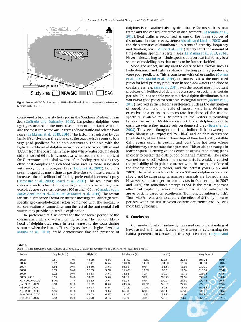
Fig. 6. Proposed SAC for T. truncatus. LVH ¼ likelihood of dolphin occurrence from lowto very high (0.2e1).

G. La Manna et al. / Ocean & Coastal Management 130 (2016) 317e327 325

considered a biodiversity hot spot in the Southern MediterraneanSea (Goffredo and Dubinsky, 2013). Lampedusa dolphins weretightly associated to the most coastal part of the island, which isalso themost congested one in terms of boat traffic and related boatnoise (La Manna et al., 2010, 2014). The factor first selected by ourJackknife analysiswas the distance to the coast, which seems to be avery good predictor for dolphin occurrence. The area with thehighest likelihood of dolphin occurrence was between 700 m and1370m from the coastline, in those sites wherewater column depthdid not exceed 60 m. In Lampedusa, what seems more importantfor T. truncatus is the shallowness of its feeding grounds, as theyoften host complex and rich food webs such as those associatedwith rocky reef and seagrass beds (Lloret et al., 2002). Dolphinsseem to spend as much time as possible close to those areas, as itincreases their likelihood of finding preferential (demersal) prey(Demestre et al., 2000; Bearzi et al., 2008). This result partiallycontrasts with other data reporting that this species may alsoexploit deeper sea sites, between 100 m and 400 m (Canadas et al.,2002; Azzellino et al., 2008, 2012; Marini et al., 2014). The reasonfor this discrepancy should be further investigated, although site-specific geo-morphological factors combined with the geograph-ical segregation of Lampedusa from the rest of the continental shelfwaters may provide a plausible explanation.

The preference of T. truncatus for the shallower portion of thecontinental shelf showed a monthly pattern. The reduced likeli-hood of dolphin occurrence in area nearest to the coast duringsummer, when the boat traffic usually reaches the highest level (LaManna et al., 2010), could demonstrate that the presence of

Table 6Area (in km) associated with classes of probability of dolphin occurrence as a function o

Period Very high (%) High (%) Mo

2005 9.81 1.0% 46.09 4.6% 112006 3.62 0.4% 65.41 6.6% 142007 5.84 0.6% 38.50 3.9% 632008 3.93 0.4% 56.83 5.7% 122009 6.22 0.6% 35.18 3.5% 712005e2009 3.55 0.4% 54.62 5.5% 91May 2005e2006 11.00 1.1% 34.25 3.5% 83Jun 2005e2009 0.50 0.1% 85.62 8.6% 21Jul 2005e2009 2.71 0.3% 53.47 5.4% 10Ago 2005e2009 4.16 0.4% 30.14 3.0% 62Sept 2005e2009 3.93 0.4% 63.92 6.4% 11Oct 2005e2006 2.52 0.3% 20.50 2.1% 32

dolphins is constrained also by disturbance factors such as boattraffic and the consequent effect of displacement (La Manna et al.,2013). Boat traffic is recognized as one of the major sources ofdisturbance in marine ecosystems (Abdulla and Linden, 2008) andthe characteristics of disturbance (in terms of intensity, frequencyand duration, sensu Miller et al., 2011) deeply affect the amount oftime dolphins spend in a certain area (La Manna et al., 2013, 2014).Nevertheless, failing to include specific data on boat traffic may be asource of modelling bias that needs to be further clarified.

Slope and aspect, usually used to describe local factors such ashydrodynamics and light irradiance affecting primary producers,were poor predictors. This is consistent with other studies (Gomezet al., 2008; Marini et al., 2014). In contrast, Chl-a, the most usedproxy for local primary production in open-sea waters and close tocoastal areas (e.g. Sar�a et al., 2011), was the second most importantpredictor of likelihood of dolphin occurrence, especially in certainperiods. Chl-a is not able per se to drive dolphin distribution, but itworks as a good proxy for other bio-ecological factors (Moure et al.,2012) involved in their feeding preference, such as the distributionof zooplankton and indirectly of zooplankters fish. While noextensive data exists to demonstrate broadness of the trophicspectrum available to T. truncatus in the waters surroundingLampedusa, overall Mediterranean bottlenose dolphins seem tooptimize where they mainly rely on demersal prey (Bearzi et al.,2008). Thus, even though there is an indirect link between pri-mary biomass (as expressed by Chl-a) and dolphin occurrence(mediated by at least two or three steps of their food web), satelliteChl-a seems useful in seeking and identifying hot spots wheredolphins may concentrate their presence. This could be strategic inMarine Spatial Planning actions when designing monitoring plansin order to predict the distribution of marine mammals. The samewas not true for SST, which, in the present study, weakly predictedthe probability of dolphin occurrence with the exception of one ofthe coldest months (October) and the hottest years (2007 and2009). The weak correlation between SST and dolphin occurrenceshould not be surprising, as marine mammals are homeotherms.However, some stronger correlations (as in October and in 2007and 2009) can sometimes emerge as SST is the most importanteffector of trophic dynamics of oceanic marine food webs, whichare essentially based on ectotherms (from phytoplankton to fish).Thus, MaxEnt was able to capture the effect of SST only in someperiods, when the link between dolphin occurrence and SST wasmost likely stronger.

5. Conclusion

Our modelling effort indirectly increased our understanding ofhow natural and human factors may interact in determining thehabitat preference of T. truncatus. This aspect is crucial (Ingram and

f year and month.

derate (%) Low (%) Very low (%)

1.97 11.3% 222.81 22.5% 601.71 60.6%8.34 14.9% 191.98 19.3% 583.04 58.8%.51 6.4% 153.84 15.5% 730.70 73.6%9.08 13.0% 183.51 18.5% 619.04 62.4%.34 7.2% 150.07 15.1% 729.58 73.5%.05 9.2% 203.73 20.5% 639.44 64.4%.63 8.4% 206.03 20.8% 657.48 66.3%3.57 21.5% 220.32 22.2% 472.38 47.6%3.27 10.4% 182.13 18.4% 650.81 65.6%.98 6.3% 66.11 6.7% 829.00 83.5%1.92 11.3% 158.82 16.0% 653.80 65.9%.50 3.3% 72.40 7.3% 864.47 87.1%

G. La Manna et al. / Ocean & Coastal Management 130 (2016) 317e327326

Rogan, 2002) to the planning and management of the conservationof the species under the Environmental Directives worldwide.

Present results may be well suited in the context of MarineSpatial Planning (MSP). MSP is rapidly gaining momentum(Stamoulis and Delevaux, 2015) and represents a powerful tool fordetecting when and where to initiate and undertake human ac-tivities at sea in order to ensure sustainability and economic effi-ciency. MPAs and SACs can play an important role, as they arearguably the most powerful tools available to date for containingthe ever-increasing over-exploitation of marine resources, thedegradation of marine habitats (Agardy et al., 2011), and for themaintenance and restoration of key species populations. Never-theless, MPAs/SACs may fail in their scope when the initial size anddesign are not dynamically adapted to meet ecological principlesand when consequent management measures are not properlyplanned (Mangano et al., 2015). In the waters around Lampedusa,the boundaries of the MPA and the SCI were initially designed(some decades ago) without calibrating their size and position inthe light of T. truncatus distributional range around the island. Thesemi-quantitative only-presence information provided here byMaxEnt seems sufficiently reliable in predicting the distribution ofT. truncatus around Lampedusa. Thus, our findings allow us tosuggest a SAC for bottlenose dolphins of about 710 km2 aroundLampedusa. SAC proposal was not only based on dolphin encounterrate data (Azzolin et al., 2007), but exploited valuable informationbased on the link between relative abundance and environmentalcovariates. This well responds to the request of high quality spatialdata and analysis as first step in making the practice of MSPpossible (Collie et al., 2013).

Datasets such as those found in this study may help in theaccomplishment of the second MSP step which relies on theassessment of human activities in the marine eco-space. Lamp-edusa local population, like those living on many geographicallysegregated islands worldwide, bases its local economy on bothfishing and tourism, with dolphin-watching often representing oneamong the most important components of the annual economicincome. Thus, since the modern concept of sustainability isgrounded on the assumption that ecological, economic and socialneeds (United Nations General Assembly, 1987) should all besatisfied simultaneously, a proper management plan at these lati-tudes should consider the SAC for dolphins in order to design andperiodically adjust (dynamically) the local exploitation level. Thiswould permit to reach a solution regarding two apparently con-trasting needs - biodiversity protection and economic develop-ment. Nevertheless, a coordination at the regional level amongmany institutions belonging to cross-border countries is necessaryfor increasing the efficiency of management measures. In the end,an integrated action over larger spatial scales (a portion of the Basinrather than only one island) represents the fundamental step forthe correct use of Marine Spatial Planning. In fact, tailoring MPAsand SACs to local conditions may individually solve localized,species-specific, or habitat-specific conservation problems, but thetotal sum of MPAs/SACs at the regional level within the context of awider strategic marine plan is the only path to increasing theeffectiveness of the ecosystem-based management practices(Agardy et al., 2011) at larger spatial scale. Thus this results shouldbe interpreted in the perspective of best practices, practices that,once verified their applicability at local scale, can be exported on abroader geographical scale.

Acknowledgements

This researchwas partially carried out under the auspices of LIFENAT/IT/000163, between 2005 and 2006. Special thanks to CTSAmbiente for its financial and logistic support. We wish to thank

students and volunteers for their assistance in the fieldwork.

References

Abdulla, A., Linden, O. (Eds.), 2008. Maritime Traffic Effects on Biodiversity in theMediterranean Sea: Review of Impacts, Priority Areas and Mitigation Measures.IUCN Centre for Mediterranean Cooperation, Malaga, Spain, p. 184.

Agardy, T., Notarbartolo di Sciara, G., Christie, P., 2011. Mind the gap: addressing theshortcomings of marine protected areas through large scale marine spatialplanning. Mar. Pol. 35 (2e35), 226e232. http://dx.doi.org/10.1016/j.marpol.2010.10.006.

Allen, M.C., Read, A.J., 2000. Habitat selection of foraging bottlenose dolphins inrelation to boat density near Clearwater, Florida. Mar. Mammal. Sci. 16,815e824.

Azzellino, A., Airoldi, S., Gaspari, S., et al., 2008. Habitat use of cetaceans along thecontinental slope and adjacent waters in the western Ligurian Sea. Deep SeaRes. Part I 55, 296e323.

Azzellino, A., Panigada, S., Lanfredi, C., et al., 2012. Predictive habitat models formanaging marine areas: spatial and temporal distribution of marine mammalswithin the Pelagos Sanctuary (Northwestern Mediterranean sea). Ocean. Coast.Manag. 67, 63e74.

Azzolin, M., Celoni, F., Galante, I., et al., 2007. Piano d'azione per il tursiope (Tursiopstruncatus) nelle isole Pelagie. Available at: http://www.provincia.agrigento.it/flex/cm/pages/ServeBLOB.php/L/IT/IDPagina/977.

Bearzi, G., Fortuna, C., Reeves, R.R., 2008. Ecology and conservation of commonbottlenose dolphins Tursiops truncatus in the Mediterranean Sea. Mam. Rev. 39(2), 92e123.

Ben Naceur, L., Gannier, A., Bradai, M.N., et al., 2004. Recensement du granddauphin Tusiops truncatus dans les eaux tunisiennes. Bull. Inst. Natl. Sci. Tech-nol. Mer Salammbo 31, 75e81.

Bohrer do Amaral, K., Alvares, D.J., Heinzelmann, L., et al., 2015. Ecological nichemodelling of Stenella dolphins (Cetartiodactyla: Delphinidae) in the south-western Atlantic ocean. J. Exp. Mar. Biol. Ecol. 472, 166e179.

Canadas, A., Sagarminaga, R., Garcıa-Tiscar, S., 2002. Cetacean distribution relatedwith depth and slope in the Mediterranean waters off southern Spain. Deep SeaRes. I 49, 2053e2073.

Canadas, A., Sagarminaga, R., De Stephanis, R., et al., 2005. Habitat selectionmodelling as a conservation tool: proposals for marine protected areas for ce-taceans in southern Spanish waters. Aq. Cons. 15, 495e521.

Canese, S., Cardinali, A., Fortuna, C.M., et al., 2006. The first known winter feedingground of fin whales (Balaenoptera physalus) in the Mediterranean Sea. J. Mar.Biol. Ass. U. K. 86 (4), 903e907.

Celoni, F., Azzolin, M., Galante, I., et al., 2007. Bottlenose dolphin (Tursiops truncatus)interaction with gill net for Mullus surmuletus at Lampedusa (Sicily). In: Euro-pean Cetacean Society Annual Conference.

Clements, G.R., Rayan, D.M., Aziz, S.A., et al., 2012. Predicting the distribution of theAsian tapir in Peninsular Malaysia using maximum entropy modelling. Integ.Zool. 7, 400e406. http://dx.doi.org/10.1111/j.1749-4877.2012.00314.x.

Collie, J.S., Adamowicz, W.L.V., Beck, M.W., et al., 2013. Marine spatial planning inpractice. Estuar. Coast. Shelf Sci. 117, 1e11.

Costa G.C., Nogueira C., Machado R.B., et al., 2009. Sampling bias and the use ofecological niche modelling in conservation planning: a field evaluation in abiodiversity hotspot. DOI 10.1007/s10531-009-9746-8.

Davis, R.W., Ortega-Ortiz, J.G., Ribic, C.A., et al., 2002. Cetacean habitat in thenorthern oceanic Gulf of Mexico. Deep Sea Res. 49, 121e143.

Demestre, M., Sanchez, P., Abell�oP, 2000. Demersal fish assemblages and habitatcharacteristics on the continental shelf and upper slope of the north-westernMediterranean. J. Mar. Biol. Ass. U.K. 80, 981e988.

Edren, S.M.C., Wisz, M.S., Teilmann, J., et al., 2010. Modelling spatial patterns inharbor porpoise satellite telemetry data using maximum entropy. Ecography33, 698e708.

Elith, J., Graham, C.H., Anderson, R.P., et al., 2006. Novel methods improve predic-tion of species' distributions from occurrence data. Ecography 29, 129e151.

Elith, J., Phillips, S.J., Hastie, T., et al., 2011. A statistical explanation of MaxEnt forecologists. Div. Distr. 17, 43e57.

European Commission, 2011. Guidelines for the Establishment of the Natura 2000Network in the Marine Environment (Application of the Habitats and BirdsDirectives).

Fourcade, Y., Engler, J.O., R€odder, D., et al., 2014. Mapping species distributions withMAXENT using a geographically biased sample of presence data: a performanceassessment of methods for correcting sampling bias. PLoS ONE 9 (5), 97e122.http://dx.doi.org/10.1371/journal.pone.0097122.

Goffredo, S., Dubinsky, Z., 2013. The Mediterranean Sea: its History and PresentChallenges. Springer Science & Business Media, p. 678.

Gomez de Segura, A., Hammond, P.S., Raga, J.A., 2008. Influence of environmentalfactors on small cetacean distribution in the Spanish Mediterranean. J. Mar. Biol.Ass. U. K. 88 (6), 1185e1192.

Gristina, M., Bahri, T., Fiorentino, F., et al., 2006. Comparison of demersal fish as-semblages in three areas of the Strait of Sicily under different trawling pressure.Fish. Res. 81, 0e71.

Guisan, A., Thuiller, W., 2005. Predicting species distribution: offering more thansimple habitat models. Ecol. Lett. 8, 993e1009.

Halpern, B., Frazier, M., Potapenko, J., et al., 2015. Spatial and temporal changes incumulative human impacts on the world's ocean. Nat. Commun. 6.

G. La Manna et al. / Ocean & Coastal Management 130 (2016) 317e327 327

Hastie, G.D., Swift, R.J., Slesser, G., Thompson, P.M., Turrell, W.R., 2005. Environ-mental models for predicting oceanic dolphin habitat in the Northeast Atlantic.ICES J. Mar. Sci. 62, 760e770.

Ingram, S., Rogan, E., 2002. Identifying critical areas and habitat preferences ofbottlenose dolphins Tursiops truncatus. Mar. Ecol. Prog. Ser. 244, 247e255.

Jaynes, E.T., 1989. Papers on Probability, Statistics, and Statistical Physics. KluwerPress, Dordrecht.

La Manna, G., Cl�o, S., Papale, E., et al., 2010. Boat traffic in the Lampedusa waters(Strait of Sicily, Mediterranean Sea) and its relationship to common bottlenosedolphin Tursiops truncatus distribution. Cienc. Mar. 36, 71e81.

La Manna, G., Manghi, M., Pavan, G., et al., 2013. Behavioural strategy of commonbottlenose dolphins (Tursiops truncatus) in response to different kinds of boatsin the waters of Lampedusa Island (Italy). Aq. Cons. 23 (5), 745e757.

La Manna, G., Manghi, M., Sar�a, G., 2014. Monitoring the habitat use of commonbottlenose dolphins (Tursiops truncatus) using passive acoustics in a Mediter-ranean marine protected area. Med. Mar. Sc. 15 (2) http://dx.doi.org/10.12681/mms.561.

LEGAMBIENTE, 2009. Piano di Gestione “Isole Pelagie” POR 1999. IT.16.1.PO.011/1.11/11.2.9/0347, SIC ITA040001 “Isola di Linosa”, SIC ITA040002 “Isole di Lampedusae Lampione” e ZPS ITA040013 “Arcipelago delle Pelagie. Area marina e ter-restre”, parte I (Fase Conoscitiva). Regione Siciliana, Assessorato Territorio edAmbiente, Palermo, p. 486.

Lloret, J., Gil de Sola, L., Souplet, A., et al., 2002. Effects of large-scale habitat vari-ability on condition of demersal exploited fish in the north-western Mediter-ranean. ICES J. Mar. Sci. 59, 1215e1227.

Mangano, C., ‘Ieary, B.C.O., Mirto, S., et al., 2015. The comparative biological effectsof spatial management measures in protecting marine biodiversity: a system-atic review protocol. Environ. Evid. 4, 21. http://dx.doi.org/10.1186/s13750-015-0047-2.

Marini, C., Fossa, F., Paoli, C., et al., 2014. Predicting bottlenose dolphin distributionalong Liguria coast (northwestern Mediterranean Sea) through differentmodelling techniques and indirect predictors. J. Env. Man. 150, 9e20.

Merow, C., Smith, M.J., Silander, J.A., 2013. A practical guide to MaxEnt for modellingspecies' distributions: what it does, and why inputs and settings matter.Ecography 36, 1058e1069. http://dx.doi.org/10.1111/j.1600-0587.2013.07872.x.

Miller, A.D., Roxburgh, S.H., Shea, K., 2011. How frequency and intensity shapediversity-disturbance relationships. PNAS 108 (14), 5643e5648.

Moure, A.E., Sillero, N., Rodrigues, A., 2012. Common dolphin (Delphinus delphis)habitat preferences using data from two platforms of opportunity. Acta Oec. 38,24e32.

Pace, D.S., Pulcini, M., Triossi, F., 2003. Interactions with fisheries: modalities ofopportunistic feeding for bottlenose dolphins at Lampedusa Island. Eur. Res.Cetaceans 17, 110e114.

Pacifici, M., et al., 2015. Assessing species vulnerability to climate change. Nat. Clim.

Change 5 (3), 215e224.Pernice, G., 2002. The HRPT Station at IRMAdCNR in Mazara del Vallo for the

Acquisition and Analysis of Satellite Data in the Strait of Sicily, pp. 98e102.MedSudMed Technical Documents No. 2.

Phillips, S.J., Anderson, R.P., Schapire, R.E., 2006. Maximum entropy modelling ofspecies geographic distributions. Ecol. Model. 190, 231e259.

Phillips, S.J., Dudìk, M., 2008. Modelling of species distributions with MaxEnt: newextensions and a comprehensive evaluation. Ecography 31, 161e175.

Phillips, S.J., Dudìk, M., Elith, J., et al., 2009. Sample selection bias and presence-onlydistribution models: implications for background and pseudo-absence data.Ecol. Appl. 19, 181e197.

Pitchford, J.L., Howard, V.A., Shelley, J.K., et al., 2014. Predictive spatial modelling ofseasonal bottlenose dolphin (Tursiops truncatus) distributions in the Mississippisound. Aq. Cons. http://dx.doi.org/10.1002/aqc.2547.

Pulcini, M., Fortuna, C.M., La Manna, G., et al., 2010. GIS Spatial Analysis as man-agement tool to describe the habitat use of bottlenose dolphins in the Lamp-edusa waters (Italy): results from eleven years of observation. In: 24th AnnualConference of the European Cetacean Society.

Roberts, J.J., Best, B.D., Dunn, D.C., et al., 2010. Marine geospatial ecology tools: anintegrated framework for ecological geoprocessing with ArcGIS, Python, R,MATLAB, and Cþþ. Environ. Model. Softw. 25, 1197e1207. http://dx.doi.org/10.1016/j.envsoft.2010.03.029.

Sar�a, G., Lo Martire, M., Sanfilippo, M., et al., 2011. Impacts of marine aquaculture atlarge spatial scales: evidences from N and P catchment loading and phyto-plankton biomass. Mar. Env. Res. 71, 317e324.

Shane, S.H., 1990. Comparison of bottlenose dolphin behavior in Texas and Florida,with a critique of methods for studying dolphin behavior. In: Leatherwood, S.,Reeves, R.R. (Eds.), The Bottlenose Dolphin. Academic Press, San Diego,pp. 541e558.

Stamoulis, A., Delevaux, J.M.S., 2015. Data requirements and tools to operationalizemarine spatial planning in the United States. Ocean Coast. Manag. 116, 214e223.

Thorne, L.H., Johnston, D.W., Urban, D.L., et al., 2012. Predictive modelling of spinnerdolphin (Stenella longirostris) resting habitat in the main Hawaiian Islands. PLoSONE 7, e43167.

United Nations General Assembly, 1987. Report of the World Commission onEnvironment and Development: Our Common Future. Transmitted to theGeneral Assembly as an Annex to document A/42/427.

Wilson, B., Thompson, P.M., Hammond, P.S., 1997. Habitat use by bottlenose dol-phins, seasonal distribution and stratified movement patterns in the MorayFirth. Scotl. J. App. Ecol. 34, 1365e1374.

Yackulic, C.B., Chandler, R., Zipkin, E.F., et al., 2013. Presence-only modelling usingMAXENT: when can we trust the inferences? Meth. Ecol. Evol. 4, 236e243.http://dx.doi.org/10.1111/2041-210x12004.