predicting climate change using response theory: global … · · 2017-04-11abstract the...

J Stat Phys (2017) 166:1036–1064DOI 10.1007/s10955-016-1506-z

Predicting Climate Change Using Response Theory:Global Averages and Spatial Patterns

Valerio Lucarini1,2 · Francesco Ragone3 ·Frank Lunkeit1

Received: 22 December 2015 / Accepted: 17 March 2016 / Published online: 21 April 2016© The Author(s) 2016. This article is published with open access at Springerlink.com

Abstract The provision of accurate methods for predicting the climate response to anthro-pogenic andnatural forcings is a key contemporary scientific challenge.Using a simplified andefficient open-source general circulation model of the atmosphere featuring O(105) degreesof freedom, we show how it is possible to approach such a problem using nonequilibriumstatistical mechanics. Response theory allows one to practically compute the time-dependentmeasure supported on the pullback attractor of the climate system, whose dynamics is non-autonomous as a result of time-dependent forcings. We propose a simple yet efficient methodfor predicting—at any lead time and in an ensemble sense—the change in climate propertiesresulting from increase in the concentration of CO2 using test perturbation model runs. Weassess strengths and limitations of the response theory in predicting the changes in the glob-ally averaged values of surface temperature and of the yearly total precipitation, as well asin their spatial patterns. The quality of the predictions obtained for the surface temperaturefields is rather good, while in the case of precipitation a good skill is observed only for theglobal average. We also show how it is possible to define accurately concepts like the inertiaof the climate system or to predict when climate change is detectable given a scenario of forc-ing. Our analysis can be extended for dealing with more complex portfolios of forcings andcan be adapted to treat, in principle, any climate observable. Our conclusion is that climatechange is indeed a problem that can be effectively seen through a statistical mechanical lens,and that there is great potential for optimizing the current coordinated modelling exercisesrun for the preparation of the subsequent reports of the Intergovernmental Panel for ClimateChange.

Paper prepared for the special issue of the Journal of Statistical Physics dedicated to the 80th birthday of Y.Sinai and D. Ruelle.

B Valerio [email protected]

1 Meteorologisches Institut, CEN, University of Hamburg, Hamburg, Germany

2 Department of Mathematics and Statistics, University of Reading, Reading, UK

3 Laboratoire de Physique de l’École Normale Supérieure de Lyon, Lyon, France

123

http://crossmark.crossref.org/dialog/?doi=10.1007/s10955-016-1506-z&domain=pdf

http://orcid.org/0000-0001-9392-1471

Predicting Climate Change Using Response Theory: Global... 1037

Keywords Response theory · Climate change · Climate prediction · General circulationmodel · Pullback attractor · Green function · Climate projections

1 Introduction

The climate is a forced and dissipative nonequilibrium chaotic systemwith a complex naturalvariability resulting from the interplay of instabilities and re-equilibrating mechanisms, neg-ative and positive feedbacks, all covering a very large range of spatial and temporal scales.One of the outstanding scientific challenges of the last decades has been to attempt to providea comprehensive theory of climate, able to explain themain features of its dynamics, describeits variability, and predict its response to a variety of forcings, both anthropogenic and natural[1–3]. The study of the phenomenology of the climate system is commonly approached byfocusing on distinct aspects like:

• wave-like features such Rossby or equatorial waves, which have enormous importancein terms of predictability and transport of, e.g., energy, momentum, and water vapour;

• particle-like features such as hurricanes, extratropical cyclones, or oceanic vortices,which are of great relevance for the local properties of the climate system and its subdo-mains;

• turbulent cascades, which determine, e.g., dissipation in the boundary layer anddevelopment of large eddies through the mechanism of geostrophic turbulence.

While each of these points of view is useful and necessary, none is able to provide alone acomprehensive understanding of the properties of the climate system; see also discussion in[4].

On a macroscopic level, one can say that at zero order the climate is driven by differencesin the absorption of solar radiation across its domain. The prevalence of absorption at surfaceand at the lower levels of the atmosphere leads, through a rich portfolio of processes, tocompensating vertical energy fluxes (most notably, convective motions in the atmosphereand exchanges of infrared radiation), while the prevalence of absorption of solar radiation inthe low latitudes regions leads to the set up of the large scale circulation of the atmosphere(with the hydrological cycle playing a key role), which allows for reducing the temperaturedifferences between tropics and polar regions with respect to what would be the case inabsence of horizontal energy transfers [5,6].

It is important to stress that such organized motions of the geophysical fluids, which actas negative feedbacks but cannot be treated as diffusive Onsager-like processes, typicallyresult from the transformation of some sort of available potential into kinetic energy, whichis continuously dissipated through a variety of irreversible processes. See [7] for a detailedanalysis of the relationship between response, fluctuations, and dissipation at different scales.Altogether, the climate can be seen as a thermal engine able to transform heat intomechanicalenergy with a given efficiency, and featuring many different irreversible processes that makeit non-ideal [2,8,9].

Besides the strictly scientific aspect, much of the interest on climate research has beendriven in the past decades by the accumulated observational evidence of the human influenceon the climate system. In order to summarize and coordinate the research activities carriedon by the scientific community, the United Nations Environment Programme (UNEP) andthe World Meteorological Organization (WMO) established in 1988 the IntergovernmentalPanel on Climate Change (IPCC). The IPCC reports, issued periodically about every 5 years,provide systematic reviews of the scientific literature on the topic of climate dynamics,

123

1038 V. Lucarini et al.

with special focus on global warming and on the socio-economic impacts of anthropogenicclimate change [10–12]. Along with such a review effort, the IPCC defines standards forthe modellistic exercises to be performed by research groups in order to provide projectionsof future climate change with numerical models of the climate system. A typical IPCC-likeclimate change experiment consists in simulating the system in a reference state (a stationarypreindustrial state with fixed parameters, or a realistic simulation of the present-day climate),raising the CO2 concentration (as well as, in general, the concentration of other greenhousegases such as methane) in the atmosphere following a certain time modulation within a giventime window, and then fixing the CO2 concentration to a final value, in order to observethe relaxation of the system to a new stationary state. Each time-modulation of the CO2

forcing defines a scenario, and it is a representation of the expected change in the CO2

concentration resulting from a specific path of industrialization and change in land use. Notethat the attribution of unusual climatic conditions to specific climate forcing is far from beinga trivial matter [13,14].

While much progress has been achieved, we are still far from having a conclusive frame-work of climate dynamics. One needs to consider that the study of climate faces, on top ofall the difficulties that are intrinsic to any nonequilibrium system, the following additionalaspects that make it especially hard to advance its understanding:

• the presence of well-defined subdomains—the atmosphere, the ocean, etc.—featuringextremely different physical and chemical properties, dominating dynamical processes,and characteristic time-scales;

• the complex processes coupling such subdomains;• the presence of a continuously varying set of forcings resulting from, e.g., the fluctuations

in the incoming solar radiation and the processes—natural and anthropogenic—alteringthe atmospheric composition;

• the lack of scale separation between different processes, which requires a profound revi-sion of the standard methods for model reduction/projection to the slow manifold, andcalls for the unavoidable need of complex parametrization of subgrid scale processes innumerical models;

• the impossibility to have detailed and homogeneous observations of the climatic fieldswith extremely high-resolution in time and in space, and the need to integrate directand indirect measurements when trying to reconstruct the past climate state beyond theindustrial era;

• the fact that we can observe only one realization of the process.

Since the climate is a nonequilibrium system, it is far from trivial to derive its response toforcings from the natural variability realized when no time-dependent forcings are applied.This is the fundamental reason why the construction of a theory of the climate responseis so challenging [3]. As already noted by Lorenz [15], it is hard to construct a one-to-one correspondence between forced and free fluctuations in a climatic context. Followingthe pioneering contribution by Leith [16], previous attempts on predicting climate responsebased broadly on applications of the fluctuation–dissipation theorem have had some degreeof success [17–21], but, in the deterministic case, the presence of correction terms due to thesingular nature of the invariant measure make such an approach potentially prone to errors[22,23]. Adding noise in the equations in the form of stochastic forcing—as in the case ofusing stochastic parametrizations [24] in multiscale system—provides a way to regularizethe problem, but it is not entirely clear how to treat the zero noise limit. Additionally, oneshould provide a robust and meaningful derivation of the model to be used for constructingthe noise: a proposal in this direction is given in [2,25,26].

123


In this paper we want to show how climate change is indeed a well-posed problem atmathematical and physical level by presenting a theoretical analysis of how PLASIM [27], ageneral circulationmodel of intermediate complexity, responds to changes in the atmosphericcomposition mimicking increasing concentrations of greenhouse gases. We will frame theproblem of studying the statistical properties of a non-autonomous, forced and dissipativecomplex system using the mathematical construction of the pullback attractor [28–30]—seealso the closely related concept of snapshot attractor [31–34]—and will use as theoreticalframework the Ruelle response theory [22,35] to compute the effect of small time-dependentperturbations on the background state. We will stick to the linear approximation, which hasproved its effectiveness in various examples of geophysical interest [23,36]. The basic ideais to use a set of probe perturbations to derive the Green function of the system, and bethen able to predict the response of the system to a large class of forcings having the samespatial structure. In this way, the uncertainties associated to the application of the fluctuation–dissipation theorem are absent and the theoretical framework is more robust. Note that, asshown in [37], one can practically implement the response theory also to treat the nonlineareffects of the forcing.

PLASIM has O(105) degrees of freedom and provides a flexible tool for performingtheoretical studies in climate dynamics. PLASIM is much faster (and indeed simpler) thanthe state of the art climatemodels used in the IPCC reports, but provides a reasonably realisticrepresentation of atmospheric dynamics and of its interactions with the land surface and withthe mixed layer of the ocean. The model includes a suite of efficient parametrization of smallscale processes such as those relevant for describing radiative transfer, cloud formation, andturbulent transport across the boundary layer. It is important to recall that in climate science itis practically necessary and conceptually very sound to choose models belonging to differentlevels of a hierarchy of complexity [38] depending on the specific problem to be studied: themost physically comprehensive and computationally expensive model is not the best modelto be used for all purposes; see discussion in [39].

In a previous work [36] we focused on the analysis of a globally averaged observable, andwe considered amodel set-upwhere themeridional oceanic heat transportwas set to zero,withno feedback from the climate state. Such a limitation resulted in an extremely high increaseof the globally averaged surface temperature resulting from higher CO2 concentrations. Inthis paper we extend the previous analysis by using a better model set-up and by consideringa wider range of climate observables, able to provide a more complete picture of the climateresponse to CO2 concentration. In particular, we wish to show to what extent response theoryis suited for performing projections of the spatial pattern of climate change.

The paper is organized as follows. In Sect. 2 we introduce the main concepts behindthe theoretical framework of our analysis. We briefly describe the basic properties of thepullback attractor and explain its relevance in the context of climate dynamics. We thendiscuss the relevance of response theory for studying situations where the non-autonomousdynamics can be decomposed into a dominating autonomous component plus a small non-autonomous correction. In Sect. 3 we introduce the climate model used in this study, discussthe various numerical experiments and the climatic observables of our interest, and presentthe data processing methods used for predicting the climate response to forcings. In Sect. 4we present the main results of our work. We focus on two observables of great relevance,namely the surface temperature and the yearly total precipitation, and investigate the skill ofresponse theory in predicting the change in their statistical properties, exploring both changesin global quantities and spatial patterns of changes. We will also show how to flexibly useresponse theory for assessing when climate change becomes statistically significant in a

123


variety of scenarios. In Sect. 5 we summarize and discuss the main findings of this work. InSect. 6 we propose some ideas for potentially exciting future investigations.

2 Pullback Attractor and Climate Response

Since the climate system experiences forcings whose variations take place on many differenttime scales [40], defining rigorously what climate response actually is requires some care. Itseems relevant to take first a step in the direction of considering the rather natural situationwhere we want to estimate the statistical properties of complex non-autonomous dynamicalsystems.

Let us then consider a continuous-time dynamical system

x = F(x, t) (1)

on a compact manifold Y ⊂ Rd , where x(t) = φ(t, t0)x(t0), with x(t = t0) = xin ∈ Y

initial condition and φ(t, t0) is defined for all t ≥ t0 with φ(s, s) = 1. The two-time evolutionoperator φ generates a two-parameter semi-group. In the autonomous case, the evolutionoperator generates a one-parameter semigroup, because of time translational invariance, sothat φ(t, s) = φ(t − s) ∀t ≥ s. In the non-autonomous case, in other terms, there is anabsolute clock. We want to consider forced and dissipative systems such that with probabilityone initial conditions in the infinite past are attracted at time t towardsA(t), a time-dependentfamily of geometrical sets. In more formal terms, we say a family of objects ∪t∈RA(t) inthe finite-dimensional, complete metric phase space Y is a pullback attractor for the systemx = F(x, t) if the following conditions are obeyed:

• ∀t ,A(t) is a compact subset ofY which is covariant with the dynamics, i.e.φ(s, t)A(t) =A(s), s ≥ t .

• ∀t limt0→−∞ dY (φ(t, t0)B,A(t)) = 0 for a.e. measurable set B ⊂ Y .where dY (P, Q) is the Hausdorff semi-distance between the P ⊂ Y and Q ⊂ Y . We havethat dY (P, Q) = supx∈P dY (x, Q), with dY (x, Q) = inf y∈Q dY (x, y). We have that, ingeneral, dY (P, Q) = dY (Q, P) and dY (P, Q) = 0 ⇒ P ⊂ Q. See a detailed discussionof these concepts in, e.g., [28–30]. Note that a substantially similar construction, the snap-shot attractor, has been proposed and fruitfully used to address a variety of time-dependentproblems, including some of climatic relevance [31–34].

In some cases, the geometrical setA(t) supports a useful measureμt (dx). Such a measurecan be obtained as evolution at time t through the Ruelle–Perron–Frobenius operator [41]of the Lebesgue measure supported on B in the infinite past, as from the conditions above.Proposing a minor generalization of the chaotic hypothesis [42], we assume that when con-sidering sufficiently high-dimensional, chaotic and non-autonomous dissipative systems, atall practical levels—i.e. when one considers macroscopic observables—the correspondingmeasureμt (dx) constructed as above is of the SRB type. This amounts to the fact that we canconstruct at all times t a meaningful (time-dependent) physics for the system. Obviously, inthe autonomous case, and under suitable conditions—e.g. in the case of of Axiom A systemor taking the point of view of the chaotic hypothesis—A(t) = � is the attractor of the system(where the t-dependence is dropped), which supports the SRB invariant measure μ(dx).

Note that whenwe analyze the statistical properties of a numericalmodel describing a non-autonomous forced and dissipative system, we often follow—sometimes inadvertently—aprotocol that mirrors precisely the definitions given above. We start many simulations inthe distant past with initial conditions chosen according to an a-priori distribution. After a

123


sufficiently long time, related to the slowest time scale of the system, at each instant thestatistical properties of the ensemble of simulations do not depend anymore on the choice ofthe initial conditions. A prominent example of this procedure is given by how simulations ofpast and historical climate conditions are performed in the modeling exercises such as thosedemanded by the IPCC [10–12], where time-dependent climate forcings due to changes ingreenhouse gases, volcanic eruptions, changes in the solar irradiance, and other astronomicaleffects are taken into account for defining the radiative forcing to the system. Note thatfuture climate projections are always performed using as initial conditions the final states ofsimulations of historical climate conditions, with the result that the covariance properties ofthe A(t) set are maintained.

Computing the expectation value of measurable observables for the time dependent mea-sure μt (dx) resulting from the evolution of the dynamical system given in Eq. 1 is in generalfar from trivial and requires constructing a very large ensemble of initial conditions in theLebesgue measurable set B mentioned before. Moreover, from the theory of pullback attrac-tors we have no real way to predict the sensitivity of the system to small changes in thedynamics.

The response theory introduced by Ruelle [22,35] (see also extensions and a differentpoint of view summarized in, e.g. [43]) allows for computing the change in the measure ofan Axiom A system resulting from weak perturbations of intensity ε applied to the dynamicsin terms of the properties of the unperturbed system. The basic concept behind the Ruelleresponse theory is that the invariant measure of the system, despite being supported on astrange geometrical set, is differentiable with respect to ε. See [44] for a discussion on theradius of convergence (in terms of ε) of the response theory.

In this case, instead, our focus is on saying that the Ruelle response theory allows forconstructing the time-dependent measure of the pullback attractor μt (dx) by computing thetime-dependent corrections of the measure with respect to a reference state. In particular, letus assume that we can write

x = F(x, t) = F(x) + εX (x, t) (2)

where |εX (x, t)| � |F(x)| ∀t ∈ R and ∀x ∈ Y , so that we can treat F(x) as the backgrounddynamics and εX (x, t) as a perturbation. Under appropriate mild regularity conditions, itis possible to perform a Schauder decomposition [45] of the forcing, so that we expressX (x, t) = ∑∞

k=1 Xk(x)Tk(t). Therefore, we restrict our analysis without loss of generalityto the case where F(x, t) = F(x) + εX (x)T (t).

One can evaluate the expectation value of a measurable observable �(x) on the timedependent measure μt (dx) of the system given in Eq. 1 as follows:

∫

μt (dx)�(x) = 〈�〉ε(t) = 〈�〉0 +∞∑

j=1

ε j 〈�〉( j)0 (t), (3)

where 〈�〉0 = ∫μ(dx)�(x) is the expectation value of � on the SRB invariant measure

μ(dx) of the dynamical system x = F(x). Each term 〈�〉( j)0 (t) can be expressed as time-

convolution of the j th order Green function G( j)� with the time modulation T (t):

〈�〉( j)0 (t) =∫ ∞

−∞dτ1 . . .

∫ ∞

−∞dτnG

( j)� (τ1, . . . , τ j )T (t − τ1) . . . T (t − τ j ). (4)

123


At each order, the Green function can be written as:

G( j)� (τ1, . . . , τ j ) =

∫

μ(dx)�(τ j − τ j−1) . . . �(τ1)�Sτ10 . . . S

τ j−10 �S

τ j0 �(x), (5)

where �(•) = X · ∇(•) and St0(•) = exp(t F · ∇)(•) is the unperturbed evolution operatorwhile the Heaviside � terms enforce causality. In particular, the linear correction term canbe written as:

〈�〉(1)0 (t),=∫

μ(dx)∫ ∞

0dτ�Sτ

0�(x)T (t − τ) =∫ ∞

−∞dτG(1)

� (τ )T (t − τ), (6)

while, considering the Fourier transform of Eq. 6, we have:

〈�〉(1)0 (ω) = χ(1)� (ω)T (ω), (7)

where we have introduced the susceptibility χ(1)� (ω) = F[G(1)

� ], defined as the Fourier

transform of the Green function G(1)� (t). Under suitable integrability conditions, the fact

that the Green function G(t) is causal is equivalent to saying that its susceptibility obeys theso-called Kramers–Kronig relations [23,46], which provide integral constraints linking itsreal and imaginary part, so that χ(1)(ω) = iP(1/ω) � χ(1)(ω), where i = √−1, � indicatesthe convolution product, and P indicates that integration by parts is considered. See alsoextensions to the case of higher order susceptibilities in [37,47–49].

As discussed in [2,23,36], the Ruelle response theory provides a powerful language forframing the problem of the response of the climate system to perturbations. Clearly, givena vector flow F(x, t), it is possible to define different background states, corresponding todifferent reference climate conditions, depending on how we break up F(x, t) into the twocontributions F(x) and εX (x, t) in the right hand side of Eq. 2. Nonetheless, as long as theexpansion is well defined, the sum given in Eq. 3 does not depend on the reference state. Ofcourse, a wise choice of the reference dynamics leads to faster convergence.

Note that once we define a background vector flow F(x) and approximate its invariantmeasure μ(dx) by performing an ensemble of simulations, by usingEqs. 3–6we can constructthe time dependent measure μt (dx) for many different choices of the perturbation fieldεX (x, t), as long aswe arewithin the radius of convergence of the response theory. Instead, inorder to construct the time dependentmeasure following directly the definition of the pullbackattractor, we need to construct a different ensemble of simulations for each choice of F(x, t).

One needs to note that constructing directly the response operator using the Ruelle for-mula given in Eq. 6 is indeed challenging, because of the different difficulties associatedto the contribution coming from the unstable and stable directions [50]; nonetheless, recentapplications of adjoint approaches [51] seem quite promising [52].

Instead, starting from Eqs. 6 and 7, it is possible to provide a simple yet general methodfor predicting the response the system for any observable � at any finite or infinite timehorizon t for any time modulation T (t) of the vector field X (x), if the corresponding Greenfunction or, equivalently, the susceptibility, is known. Moreover, given a specific choice ofT (t) and measuring 〈�〉(1)0 (t) from a set of experiments, the same equations allow one toderive the Green function. Therefore, using the output of a specific set of experiments, weachieve predictive power for any temporal pattern of the forcing X (x). In other terms, fromthe knowledge of the time dependent measure of one specific pullback attractor, we canderive the time dependent measures of a family of pullback attractors. We will follow thisapproach in the analysis detailed below. While the methodology is almost trivial in the linearcase, it is in principle feasible also when higher order corrections are considered, as long asthe response theory is applicable [37,48,49].

123


We remark that in some cases divergence in the response of a chaotic system can beassociated to the presence of slow decorrelation for the measurable observable in the back-ground state, which, as discussed in e.g. [53], can be related to the presence of nearby criticaltransitions. Indeed, we have recently investigated such an issue in [54], thus providing thestatistical mechanical embedding for the classical problem of multistability of the Earth’ssystem, which had been previously studied using macroscopic thermodynamics in [55–57].

3 A Climate Model of Intermediate Complexity: The PlanetSimulator—PLASIM

The Planet Simulator (PLASIM) is a climate model of intermediate complexity, freely avail-able upon request to the group of Theoretical Meteorology at the University of Hamburgand includes a graphical user interface facilitating its use. By intermediate complexity wemean that the model is gauged in such a way to be parsimonious in terms of computationalcost and flexible in terms of the possibility of exploring widely differing climatic regimes[39]. Therefore, the most important climatic processes are indeed represented, and the modelis complex enough to feature essential characteristics of high-dimensional, dissipative, andchaotic systems, as the existence of a limited horizon of predictability due to the presenceof instabilities in the flow. Nonetheless, one has to sacrifice the possibility of using the mostadvanced parametrizations for subscale processes and cannot use high resolutions for thevertical and horizontal directions in the representation of the geophysical fluids. Therefore,we are talking of a modelling strategy that differs from the conventional approach aimingat achieving the highest possible resolution in the fluid fields and the highest precision inthe parametrization of the highest possible variety of subgrid scale processes [12], but ratherfocuses on trying to reduce the gap between the modelling and the understanding of thedynamics of the geophysical flows [58].

The dynamical core of PLASIM is based on the Portable University Model of theAtmosphere PUMA [59]. The atmospheric dynamics is modelled using the primitive equa-tions formulated for vorticity, divergence, temperature and the logarithm of surface pressure.Moisture is included by transport of water vapour (specific humidity). The governing equa-tions are solved using the spectral transform method [60,61]. In the vertical, non-equallyspaced sigma (pressure divided by surface pressure) levels are used. The parametrization ofunresolved processes consists of long- [62] and short- [63] wave radiation, interactive clouds[64–66], moist [67,68] and dry convection, large-scale precipitation, boundary layer fluxesof latent and sensible heat and vertical and horizontal diffusion [69–72]. The land surfacescheme uses five diffusive layers for the temperature and a bucket model for the soil hydrol-ogy. The oceanic part is a 50mmixed-layer (swamp) ocean, which includes a thermodynamicsea ice model [73].

The horizontal transport of heat in the ocean can either be prescribed or parametrized byhorizontal diffusion. While in [36] the ocean transport was set to zero, in the experimentsperformed here we choose the second option, because having even a severely simplifiedrepresentation of the feedbacks associated to the large scale heat transport performed bythe ocean improves the realism of the response of the system. We remind that the oceancontributes to about 30% of the total meridional heat transport in the present climate [6,74,75]. A detailed study of the impact of changing oceanic heat transports on the dynamics andthermodynamics of the atmosphere can be found in [76].

123


0 100 200 300-80

-60

-40

-20

0

20

40

60

80(a) (b)

(c)

200

220

240

260

280

300

0 100 200 300-80

-60

-40

-20

0

20

40

60

80

0

1000

2000

3000

4000

5000

6000

-80 -60 -40 -20 0 20 40 60 80210

230

250

270

290

310

0

400

800

1200

1600

2000

2400

2800

3200

3600

4000

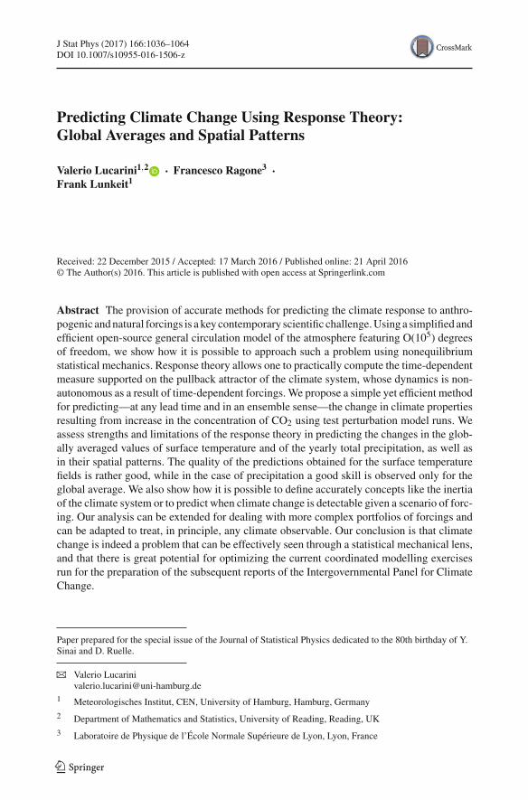
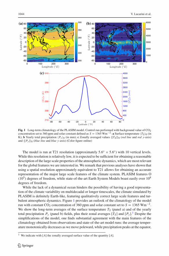
Fig. 1 Long-term climatology of the PLASIM model. Control run performed with background value of CO2concentration set to 360 ppm and solar constant defined as S = 1365Wm−2: a Surface temperature 〈TS〉0 (inK); b Yearly total precipitation 〈Py〉0 (in mm); c Zonally averaged values 〈[TS ]〉0 (red line and red y-axis)and 〈[Py ]〉0 (blue line and blue y-axis) (Color figure online)

The model is run at T21 resolution (approximately 5.6◦ × 5.6◦) with 10 vertical levels.While this resolution is relatively low, it is expected to be sufficient for obtaining a reasonabledescription of the large scale properties of the atmospheric dynamics, which aremost relevantfor the global features we are interested in.We remark that previous analyses have shown thatusing a spatial resolution approximately equivalent to T21 allows for obtaining an accuraterepresentation of the major large scale features of the climate system. PLASIM features O(105) degrees of freedom, while state-of-the-art Earth System Models boast easily over 108

degrees of freedom.While the lack of a dynamical ocean hinders the possibility of having a good representa-

tion of the climate variability on multidecadal or longer timescales, the climate simulated byPLASIM is definitely Earth-like, featuring qualitatively correct large scale features and tur-bulent atmospheric dynamics. Figure 1 provides an outlook of the climatology of the modelrun with constant CO2 concentration of 360 ppm and solar constant set to S = 1365 Wm−2.We show the long-term averages of the surface temperature TS (panel a) and of the yearlytotal precipitation Py (panel b) fields, plus their zonal averages [TS] and [Py].1 Despite thesimplifications of the model, one finds substantial agreement with the main features of theclimatology obtained from observations and state-of-the-art model runs: the average temper-aturemonotonically decreases as wemove poleward, while precipitation peaks at the equator,

1 We indicate with [A] the zonally averaged surface value of the quantity [A].

123


as a result of the large scale convection corresponding to the intertropical convergence zone(ICTZ), and features two secondary maxima at the mid latitudes of the two hemispheres, cor-responding to the areas of the so-called storm tracks [6]. As a result of the lack of a realisticoceanic heat transport and of too low resolution in the model, the position to the ICTZ is abit unrealistic as it is shifted southwards compared to the real world, with the precipitationpeaking just south of the equator instead of few degrees north of it.

Beside standard output, PLASIM provides comprehensive diagnostics for the nonequi-librium thermodynamical properties of the climate system and in particular for local andglobal energy and entropy budgets. PUMA and PLASIM have already been used for sev-eral theoretical climate studies, including a variety of problems in climate response theory[2,36], climate thermodynamics [77,78], analysis of climatic tipping points [54,55], and inthe dynamics of exoplanets [56,57].

3.1 Experimental Setting

We want to perform predictions on the climatic impact of different scenarios of increase inthe CO2 concentration with respect to a baseline value of 360 ppm, focusing on observables� of obvious climatic interest such as, e.g. the globally averaged surface temperature TS . Wewish to emphasise that most state-of-the-art general circulation models feature an imperfectclosure of the global energy budget of the order of 1 Wm−2 for standard climate conditions,due to inaccuracies in the treatment of the dissipation of kinetic energy and the hydrologicalcycle [2,75,79,80]. Instead, PLASIM has been modified in such a way that a more accuraterepresentation of the energy budget is obtained, even in rather extreme climatic conditions[55–57]. Therefore, we are confident of the thermodynamic consistency of our model, whichis crucial for evaluating correctly the climate response to radiative forcing resulting fromchanges in the opacity of the atmosphere.

We proceed step-by-step as follows:

• We take as dynamical system x = F(x) the spatially discretized version of the partialdifferential equations describing the evolution of the climate variables in a baseline sce-nario with set boundary conditions and set values for, e.g., the CO2 = 360 ppm baselineconcentration and the solar constant S = 1365 Wm−2. We assume, for simplicity, thatsystem does not feature daily or seasonal variations in the radiative input at the top of theatmosphere. We run the model for 2400 years in order to construct a long control run.Note that the model relaxes to its attractor with an approximate time scale of 20–30 years.

• We study the impact of perturbations using a specific test case. We run a first set ofN = 200 perturbed simulations, each lasting 200 years, and each initialized with thestate of the model at year 200 + 10k, k = 1, . . . , 200. We choose as perturbation fieldX (x) the additional convergence of radiative fluxes due to changes in the atmosphericCO2 concentration. Therefore, such a perturbation field has non-zero components onlyfor the variables directly affected by such forcings, i.e. the values of the temperatures atthe resolved grid points of the atmosphere and at the surface. In each of these simulationwe perturbed the vector flow by doubling instantaneously the CO2 concentration. Thiscorresponds to having x = F(x) → x = F(x) + ε�(t)X (x). Note that the forcing iswell known to scale proportionally to the logarithm of the CO2 concentration [6].

• By plugging T (t) = Ta(t) = �(t) into Eq. 6, we have that :

d

dt〈�〉(1)0 (t) = εG(1)

� (t) (8)

123


We estimate 〈�〉(1)0 (t) by taking the average of response of the system over a possiblylarge number of ensemble members, and use the previous equation to derive our estimateof G(1)

� (t), by assuming linearity in the response of the system. In what follows, wepresent the results obtained using all the available N = 200 ensemble members, plus,in some selected cases, showing the impact of having a smaller number (N = 20) ofensemble members.It is important to emphasize that framing the problem of climate change using the formal-ism of response theory gives usways for providing simple yet useful formulas for definingprecisely the climate sensitivity �� for a general observable �, as �� = �{χ(1)

� (0)}.Furthermore, if we consider perturbation modulated by a Heaviside distribution, we havethe additional simple and useful relation:

�� = 2

πε

∫

dω′�{〈�〉(1)0 (ω′)}, (9)

which relates climate response at all frequencies to its sensitivity, as resulting from thevalidity of the Kramers–Kronig relations.We remark that using a given set of forced experiments it is possible to derive informationon the climate response to the given forcing for as many climatic observables as desired.It is important to note that, for a given finite intensity ε of the forcing, the accuracyof the linear theory in describing the full response depends also on the observable ofinterest. Moreover, the signal to noise ratio and, consequently, the time scales over whichpredictive skill is good may change a lot from variable to variable.

• We want to be able to predict at finite and infinite time the response of the system tosome other pattern of CO2 forcing. Following [36], we choose as a pattern of forcing oneof the classic IPCC scenarios, namely a 1% yearly increase of the CO2 concentrationup to its doubling, and we perform a set of additional N = 200 perturbed simulationsperformed according to such a protocol. Since, as mentioned above, the radiative forcingis proportional to the logarithm of the CO2 concentration, this corresponds to choosinga new time modulation that can be approximated as a linear ramp of the form

T τb (t) = εt/τ, 0 ≤ t ≤ τ, T τ

b (t) = 1, t > τ, (10)

where τ = 100 log(2) years∼ 70 years is the doubling time. Therefore, for each observ-able � we compare the result of convoluting the estimate of the Green function obtainedin the previous step with time modulation Tb(t)with the ensemble average obtained fromthe new set of simulations.

4 Results

The response theory sketched above allows us in principle to study the change in the statisticalproperties of any well-behaved, smooth enough observable. Nonetheless, problems naturallyemerge when we consider finite time statistics, finite number of ensemble members, andfinite precision approximations of the response operators. The Green functions of interest arederived using Eq. 8 as time derivative of the ensemble averaged time series of the observedresponse to the probe forcing whose time modulation is given by the Heaviside distribution.Clearly, the response is not smooth unless the ensemble size N → ∞. Therefore, takingnumerically the time derivative leads to having a very noisy estimate of the Green function,which might also depend heavily on the specific procedure used for computing the discrete

123


derivative. This might suggest that the procedure is not robust. Instead, we need to keepin mind that we aim at using the Green function exclusively as a tool for predicting theclimate response. Therefore, if we convolute with the Green function with a sufficientlysmooth modulating factor T (t) as in Eq. 6, the small time scales fluctuations of the Greenfunction, albeit large in size, become of no relevance, because they are averaged out. This isfurther eased if, instead of looking for predictions valid for observables defined at the highestpossible time resolution of our model, we concentrate of suitably time averaged quantities.Clearly, while it is in principle possible to define mathematically the climate response on thetime scale of, e.g., one second, this has no real physical relevance. Looking at the asymptoticbehaviour of the susceptibility χ

(1)� (ω) for ω → ∞ it is possible to derive what is, depending

on the signal-to-noise ratio, the time scale over which we can expect to be able to performmeaningful predictions; see discussion in [36].

In order to provide an overlook of the practical potential of the response theory in address-ing the problem of climate change, we have decided to focus on two climatological quantitiesof general interest, namely the yearly averaged surface temperature TS and the yearly total pre-cipitation Py . Such quantities have obvious relevance for basically any possible impact studyof climate change, and, while there is muchmore in climate change than studying the changesin TS and Py , these are indeed thefirst quantities one considerswhenbenchmarking the perfor-mance of a climatemodel andwhen assessingwhether climate change signals can be detected.

Another issue one needs to address is the role of the spatial patterns of change in theconsidered quantities. The change in the globally average surface temperature {TS}2 hasundoubtedly gained prominence in the climate change debate and in the IPCC negotiationstargets are tailored according to such an indicators.Nonetheless, the impacts of climate changeare in fact local and one needs to investigate the spatial patterns of the change signals [12].Evidently, one expects that coarse grained (in space) quantities will have a better signal-to-noise ratio and will allow for performing higher precision climate projection using responsetheory. On the other side, the performance of linear response theory at local scale mightbe hindered by the presence of local strongly nonlinear feedbacks, such as the ice-albedofeedback, which have less relevance when spatial averaging is performed. In what follows,we will consider observables constructed from the spatial fields of TS and Py by performingdifferent levels of coarse graining.Wewill begin by looking into globally averaged quantities,and then address the problem of predicting the spatial patterns of climate change.

4.1 Globally Averaged Quantities

We begin our investigation by focusing on the globally averaged surface temperature {TS}and the globally averaged yearly total precipitation {Py}. In what follows, we perform theanalysis using the model output at the highest available resolution (1 day) but present, forsake of convenience and since we indeed focus on yearly quantities, data where a 1-yearband pass filtering is performed.

4.1.1 From Green Functions to Climate Predictions

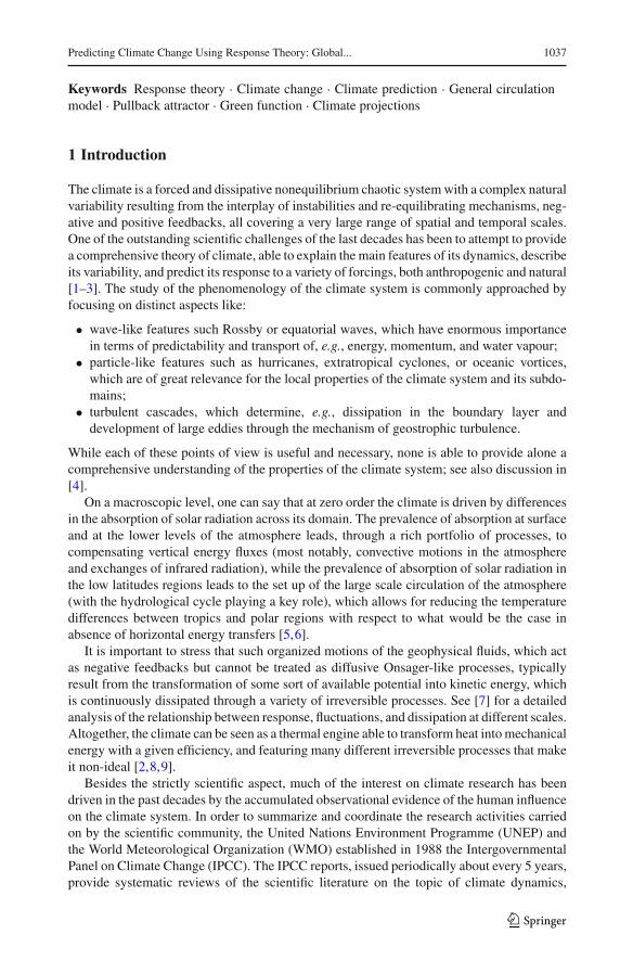
Figure 2 shows the ensemble average performed over N = 200 members of the change of〈{TS}〉 (panel a) and 〈{Py}〉 (panel b) as a result of the instantaneous doubling of the CO2

concentration described in the previous section. We find that the asymptotic change in thesurface temperature is given by the equilibrium climate sensitivity ECS = �{TS} ∼ 4.9

2 We indicate with {A} the globally averaged surface value of the quantity A.

123


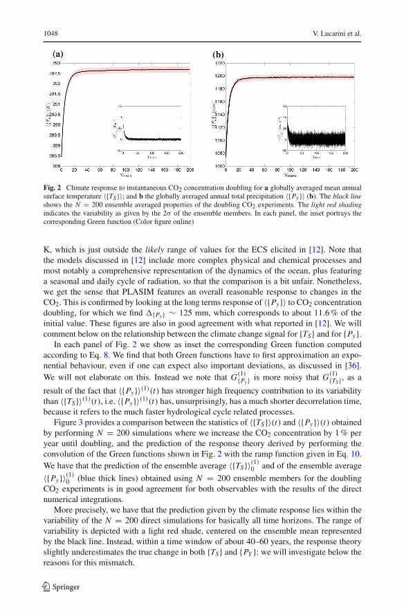
Fig. 2 Climate response to instantaneous CO2 concentration doubling for a globally averaged mean annualsurface temperature 〈{TS}〉; and b the globally averaged annual total precipitation 〈{Py}〉 (b). The black lineshows the N = 200 ensemble averaged properties of the doubling CO2 experiments. The light red shadingindicates the variability as given by the 2σ of the ensemble members. In each panel, the inset portrays thecorresponding Green function (Color figure online)

K, which is just outside the likely range of values for the ECS elicited in [12]. Note thatthe models discussed in [12] include more complex physical and chemical processes andmost notably a comprehensive representation of the dynamics of the ocean, plus featuringa seasonal and daily cycle of radiation, so that the comparison is a bit unfair. Nonetheless,we get the sense that PLASIM features an overall reasonable response to changes in theCO2. This is confirmed by looking at the long terms response of 〈{Py}〉 to CO2 concentrationdoubling, for which we find �{Py } ∼ 125 mm, which corresponds to about 11.6% of theinitial value. These figures are also in good agreement with what reported in [12]. We willcomment below on the relationship between the climate change signal for {TS} and for {Py}.

In each panel of Fig. 2 we show as inset the corresponding Green function computedaccording to Eq. 8. We find that both Green functions have to first approximation an expo-nential behaviour, even if one can expect also important deviations, as discussed in [36].We will not elaborate on this. Instead we note that G(1)

{Py} is more noisy that G(1){TS}, as a

result of the fact that 〈{Py}〉(1)(t) has stronger high frequency contribution to its variabilitythan 〈{TS}〉(1)(t), i.e. 〈{Py}〉(1)(t) has, unsurprisingly, has a much shorter decorrelation time,because it refers to the much faster hydrological cycle related processes.

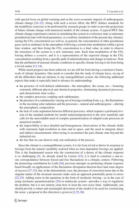
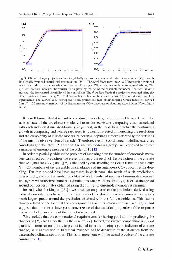
Figure 3 provides a comparison between the statistics of 〈{TS}〉(t) and 〈{Py}〉(t) obtainedby performing N = 200 simulations where we increase the CO2 concentration by 1% peryear until doubling, and the prediction of the response theory derived by performing theconvolution of the Green functions shown in Fig. 2 with the ramp function given in Eq. 10.We have that the prediction of the ensemble average 〈{TS}〉(1)0 and of the ensemble average

〈{Py}〉(1)0 (blue thick lines) obtained using N = 200 ensemble members for the doublingCO2 experiments is in good agreement for both observables with the results of the directnumerical integrations.

More precisely, we have that the prediction given by the climate response lies within thevariability of the N = 200 direct simulations for basically all time horizons. The range ofvariability is depicted with a light red shade, centered on the ensemble mean representedby the black line. Instead, within a time window of about 40–60 years, the response theoryslightly underestimates the true change in both {TS} and {PY }: we will investigate below thereasons for this mismatch.

123


Fig. 3 Climate change projections for a the globally averaged mean annual surface temperature 〈{TS}〉; and bthe globally averaged annual total precipitation 〈{Py}〉. The black line shows the N = 200 ensemble averagedproperties of the experiments where we have a 1% per year CO2 concentration increase up to doubling. Thelight red shading indicates the variability as given by the 2σ of the ensemble members. The blue shadingindicates the interannual variability of the control run. The thick blue line is the projection obtained using theGreen functions derived using N = 200 ensemble members of the instantaneous CO2 concentration doublingexperiments. The dashed lines correspond to ten projections each obtained using Green functions derivedfrom N = 20 ensemble members of the instantaneous CO2 concentration doubling experiments (Color figureonline)

It is well known that it is hard to construct a very large set of ensemble members in thecase of state-of-the-art climate models, due to the exorbitant computing costs associatedwith each individual run. Additionally, in general, in the modelling practise the continuousgrowth in computing and storing resources is typically invested in increasing the resolutionand the complexity of climate models, rather than populating more attentively the statisticsof the run of a given version of a model. Therefore, even in coordinated modelling exercisescontributing to the latest IPCC report, the various modelling groups are requested to delivera number of ensemble member of the order of 10 [12].

In order to partially address the problem of assessing how the number of ensemble mem-bers can affect our prediction, we present in Fig. 3 the result of the prediction of the climatechange signal for 〈{TS}〉 and 〈{Py}〉 obtained by constructing the Green function using onlyN = 20 members of the ensemble of simulations of instantaneous CO2 concentration dou-bling. Ten thin dashed blue lines represent in each panel the result of such predictions.Interestingly, each of the prediction obtained with a reduced number of ensemble membersalso agreeswith the direct numerical simulationswhenwe consider 〈{TS}〉, because the spreadaround our best estimates obtained using the full set of ensemble members is minimal.

Instead, when looking at 〈{Py}〉, we have that only some of the predictions derived usingreduced ensemble sets lie within the variability of the direct numerical simulations, with amuch larger spread around the prediction obtained with the full ensemble set. This fact isclosely related to the fact that the corresponding Green function is noisier, see Fig. 2, andsuggests that in order to have good convergence of the statistical properties of the responseoperator a better sampling of the attractor is needed.

We conclude that the computational requirements for having good skill in predicting thechanges in {Py} are harder than in the case of {TS}. Indeed, the surface temperature is a goodquantity in terms of our ability to predict it, and in terms of being a good indicator of climatechange, as it allows one to find clear evidence of the departure of the statistics from theunperturbed climate conditions. This is in agreement with the actual practice of the climatecommunity [12].

123


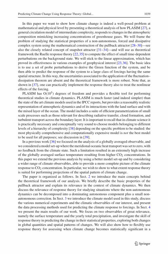
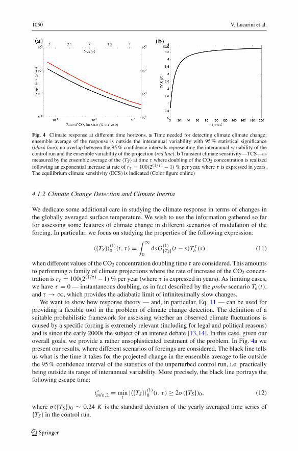
Fig. 4 Climate response at different time horizons. a Time needed for detecting climate climate change:ensemble average of the response is outside the interannual variability with 95% statistical significance(black line); no overlap between the 95% confidence intervals representing the interannual variability of thecontrol run and the ensemble variability of the projection (red line). b Transient climate sensitivity—TCS—asmeasured by the ensemble average of the 〈TS〉 at time τ where doubling of the CO2 concentration is realizedfollowing an exponential increase at rate of rτ = 100(2(1/τ) − 1) % per year, where τ is expressed in years.The equilibrium climate sensitivity (ECS) is indicated (Color figure online)

4.1.2 Climate Change Detection and Climate Inertia

We dedicate some additional care in studying the climate response in terms of changes inthe globally averaged surface temperature. We wish to use the information gathered so farfor assessing some features of climate change in different scenarios of modulation of theforcing. In particular, we focus on studying the properties of the following expression:

〈{TS}〉(1)0 (t, τ ) =∫ ∞

0dsG(1)

{TS}(t − s)T τb (s) (11)

when different values of the CO2 concentration doubling time τ are considered. This amountsto performing a family of climate projections where the rate of increase of the CO2 concen-tration is rτ = 100(2(1/τ) − 1) % per year (where τ is expressed in years). As limiting cases,we have τ = 0 — instantaneous doubling, as in fact described by the probe scenario Ta(t),and τ → ∞, which provides the adiabatic limit of infinitesimally slow changes.

We want to show how response theory — and, in particular, Eq. 11 — can be used forproviding a flexible tool in the problem of climate change detection. The definition of asuitable probabilistic framework for assessing whether an observed climate fluctuations iscaused by a specific forcing is extremely relevant (including for legal and political reasons)and is since the early 2000s the subject of an intense debate [13,14]. In this case, given ouroverall goals, we provide a rather unsophisticated treatment of the problem. In Fig. 4a wepresent our results, where different scenarios of forcings are considered. The black line tellsus what is the time it takes for the projected change in the ensemble average to lie outsidethe 95% confidence interval of the statistics of the unperturbed control run, i.e. practicallybeing outside its range of interannual variability. More precisely, the black line portrays thefollowing escape time:

tτmin,2 = mint

|〈{TS}〉(1)0 (t, τ ) ≥ 2σ({TS})0, (12)

where σ({TS})0 ∼ 0.24 K is the standard deviation of the yearly averaged time series of{TS} in the control run.

123


Nonetheless, we would like to be able to assess when not only the projected change in theensemble average is distinguishable from the statistics of the control run, but, rather, whenan actual individual simulation is incompatible with the statistics of the unperturbed climate,because we live in one of such realizations, and not on any averaged quantity. Obviously, inorder to assess this, one would require performing an ensemble of direct simulations, thusgiving no scope to any application of the response theory. We can observe, though, fromFig. 3a, that the interannual variability of the control run and the ensemble variability of theperturbed run are rather similar (being the same if no perturbation is applied). Therefore,we heuristically assume that the two confidence intervals have the same width. The red lineportrays the second escape time

tτmin,4 = mint

|〈{TS}〉(1)0 (t, τ ) ≥ 4σ({TS})0, (13)

such that for t ≥ tτmin,4 it is extremely unlikely that any realization of the climate changescenario due to a forcing of the form T τ

b perturbed run has statistics compatible with that ofthe control run. In other terms, tτmin,4 provides a robust estimate of when detection of climatechange in virtually unavoidable from a single run, while tτmin,2 gives an estimate of the timehorizon after which it makes sense to talk about climate change. We would like to remarkthat using the Green functions reconstructed from the reduced ensemble sets as shown inFig. 3, one obtains virtually indistinguishable estimates for t ≥ tτmin,2 and t ≥ tτmin,4 for allvalues of τ . This suggests that these quantities are rather robust.

Wecandetect twoapproximate scaling regimes,with changeover takingplace for rτ ∼ 1%per year.

• for large values of rτ (≥1% per year), we have that tτmin,2, tτmin,4 ∝ r−0.6

τ

• for moderate values of rτ (≤1% per year), we have that tτmin,2, tτmin,4 ∝ r−1

τ . Thelatter corresponds to the quasi-adiabatic regime and one finds that, correspondingly,tτmin,4, t

τmin,2 ∝ τ .

A quantity that has attracted considerable interest in the climate community is the so-calledtransient climate sensitivity (TCS), which, as opposed to the ECS, which looks at asymptotictemperature changes, describes the change of {TS} at the moment of CO2 concentrationdoubling following a 1% per year increase [81]. The difference between ECS and TSC givesa measure of the inertia of the climate system in reaching the asymptotic increase of {TS}realized with doubled CO2 concentration. Using response theory, we can extend the conceptof transient climate sensitivity by considering any rate of exponential increase of the CO2

concentration, as discussed in [36]. Using Eq. 11, we have that:

TCS(τ ) = 〈{TS}〉(1)0 (τ, τ ) (14)

describes the change in the expectation value of {TS} at the end of the ramp of increase ofCO2 concentration. As suggested by the argument proposed in [81], one expects that the TCSis a monotonically increasing function of τ (see Fig. 4b), and that the difference between theECS and TCS becomes very small for large values of τ , because we enter the quasi-adiabaticregime where the change in the CO2 is slower than the slowest internal time scale of thesystem.

4.1.3 A Final Remark

Wewould like tomake afinal remarkof the properties of the response of the global observables{TS} and {Py}. Looking at Figs. 2 and 3, one is unavoidably bound to observe that the

123


temporal pattern of response of {TS} and {Py} are extremely similar. In agreement with [81](see also [12]), we find that to a very good approximation the following scaling applies forall simulations:

〈{Py}〉(1)0 (t)

〈{Py}〉0 ∼ 0.025〈{TS}〉(1)0 (t)

K,

where K is one degree Kelvin. In other terms, the twoGreen functionsG(1){TS} andG

(1){Py} are, to

a very good approximation, proportional to each other when yearly averages are considered.Note that this scaling relations does not agree with the naive scaling imposed by the

Clausius–Clapeyron relation controlling the partial pressure of saturated water vapour. Infact, were the Clausius–Clapeyron scaling correct, one would have

δ〈{Py}〉(1)0 (t)

〈{Py}〉0 ∼ 0.07δ〈{TS}〉(1)0 (t)

K.

The reasons why a scaling between changes in {TS} and {Py} exists at all, and why it lookslike a modified version of a Clausius–Clapeyron-like law, are hotly debated in the literature[82–84].

4.2 Predicting Spatial Patterns of Climate Change

While there is a very strong link between the change in the globally averaged precipitationand of the globally averaged surface temperature, important differences emergewhen lookingat the spatial patterns of change of the two fields [83]. We will investigate the spatial featuresof climate response in the next subsection.

Themethods of response theory allow us to treat seamlessly also the problem of predictingthe climate response for (spatially) local observables. It is enough to define appropriately theobservable � and repeat the procedure described in Sect. 3.1. As a first step in the directionof assessing our ability to predict climate change at local scale, we concentrate the zonally(longitudinally) averaged fields [TS](λ) and [Py](λ), where we have made explicit referenceto to the dependence on the latitude λ. Studying these fields is extremely relevant because itallows us to look at the difference of the climate response at different latitudinal belts, whichare well known to have entirely different dynamical properties, and, in particular, to look atequatorial-polar contrasts.

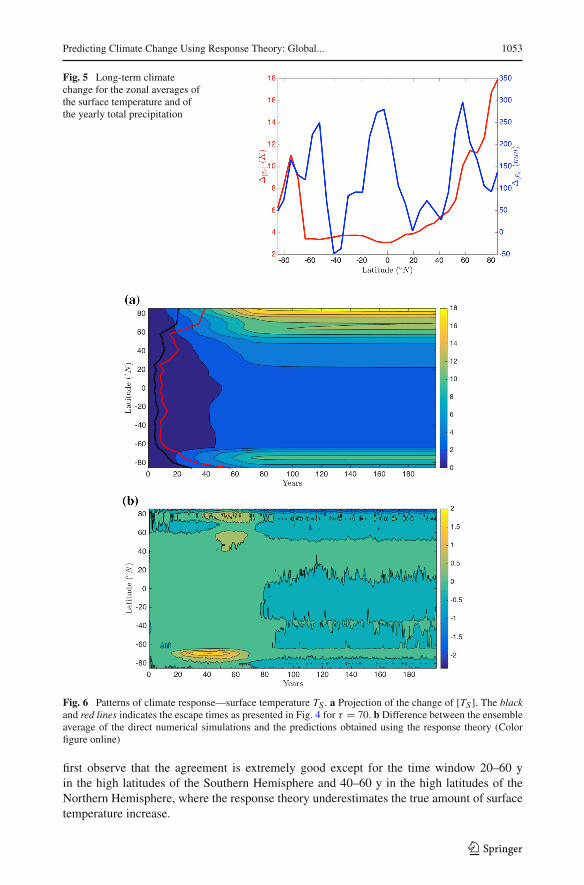
We show in Fig. 5 the long-term change in the climatology of the [TS], i.e., the climatesensitivity for each latitudinal band. We have confirmation of well-established findings: theresponse of the surface temperature ismuch stronger in the higher latitudes than in the tropicalregions, as a result of the local ice-albedo feedback and, secondarily, of the increased transportresulting from changes in the circulation. Additionally, there is a clear asymmetry betweenthe two hemispheres, with the response in the northern hemisphere being notably larger, asa result of the larger land masses [12]

In this case, we need first to construct a different Green function for each latitude from theinstantaneous CO2 doubling experiments. Then, we perform the convolution of the Greenfunctions with the same ramp function and obtaining the prediction of the response to the1% per year increase in the CO2 concentration for each latitude.

Figure 6 shows the result of our application of the response theory for predicting theresponse of the zonally averaged surface temperature to the considered forcing scenario:panel a displays the projection performed using response theory, and panel b shows thedifference between the results obtained from the actual direct numerical simulations. We

123


Fig. 5 Long-term climatechange for the zonal averages ofthe surface temperature and ofthe yearly total precipitation

Fig. 6 Patterns of climate response—surface temperature TS . a Projection of the change of [TS ]. The blackand red lines indicates the escape times as presented in Fig. 4 for τ = 70. b Difference between the ensembleaverage of the direct numerical simulations and the predictions obtained using the response theory (Colorfigure online)

first observe that the agreement is extremely good except for the time window 20–60 yin the high latitudes of the Southern Hemisphere and 40–60 y in the high latitudes of theNorthern Hemisphere, where the response theory underestimates the true amount of surfacetemperature increase.

123


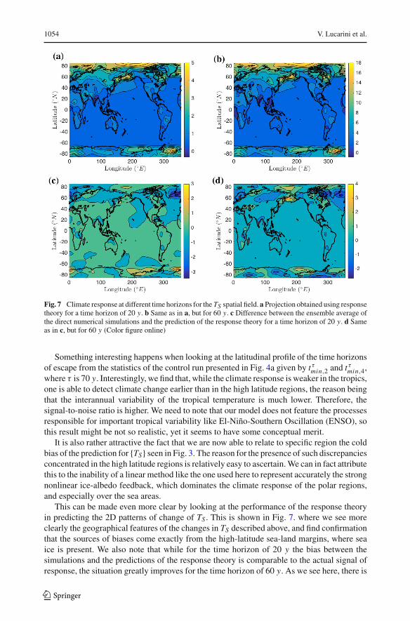
Fig. 7 Climate response at different time horizons for the TS spatial field. a Projection obtained using responsetheory for a time horizon of 20 y. b Same as in a, but for 60 y. c Difference between the ensemble average ofthe direct numerical simulations and the prediction of the response theory for a time horizon of 20 y. d Sameas in c, but for 60 y (Color figure online)

Something interesting happens when looking at the latitudinal profile of the time horizonsof escape from the statistics of the control run presented in Fig. 4a given by tτmin,2 and t

τmin,4,

where τ is 70 y. Interestingly, we find that, while the climate response is weaker in the tropics,one is able to detect climate change earlier than in the high latitude regions, the reason beingthat the interannual variability of the tropical temperature is much lower. Therefore, thesignal-to-noise ratio is higher. We need to note that our model does not feature the processesresponsible for important tropical variability like El-Niño-Southern Oscillation (ENSO), sothis result might be not so realistic, yet it seems to have some conceptual merit.

It is also rather attractive the fact that we are now able to relate to specific region the coldbias of the prediction for {TS} seen in Fig. 3. The reason for the presence of such discrepanciesconcentrated in the high latitude regions is relatively easy to ascertain.We can in fact attributethis to the inability of a linear method like the one used here to represent accurately the strongnonlinear ice-albedo feedback, which dominates the climate response of the polar regions,and especially over the sea areas.

This can be made even more clear by looking at the performance of the response theoryin predicting the 2D patterns of change of TS . This is shown in Fig. 7. where we see moreclearly the geographical features of the changes in TS described above, and find confirmationthat the sources of biases come exactly from the high-latitude sea-land margins, where seaice is present. We also note that while for the time horizon of 20 y the bias between thesimulations and the predictions of the response theory is comparable to the actual signal ofresponse, the situation greatly improves for the time horizon of 60 y. As we see here, there is

123


good hope in being able to predict quite accurately the climate response also at local scale,with no coarse graining involved, at least in the case of the TS field.

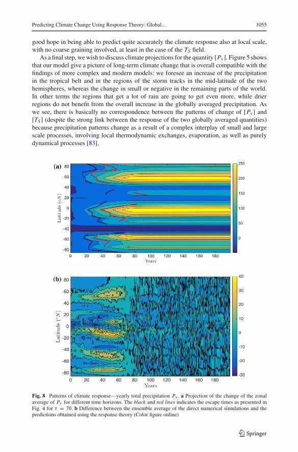
As a final step, wewish to discuss climate projections for the quantity [Py]. Figure 5 showsthat our model give a picture of long-term climate change that is overall compatible with thefindings of more complex and modern models: we foresee an increase of the precipitationin the tropical belt and in the regions of the storm tracks in the mid-latitude of the twohemispheres, whereas the change in small or negative in the remaining parts of the world.In other terms the regions that get a lot of rain are going to get even more, while drierregions do not benefit from the overall increase in the globally averaged precipitation. Aswe see, there is basically no correspondence between the patterns of change of [Py] and[TS] (despite the strong link between the response of the two globally averaged quantities)because precipitation patterns change as a result of a complex interplay of small and largescale processes, involving local thermodynamic exchanges, evaporation, as well as purelydynamical processes [83].

Fig. 8 Patterns of climate response—yearly total precipitation Py . a Projection of the change of the zonalaverage of Py for different time horizons. The black and red lines indicates the escape times as presented inFig. 4 for τ = 70. b Difference between the ensemble average of the direct numerical simulations and thepredictions obtained using the response theory (Color figure online)

123


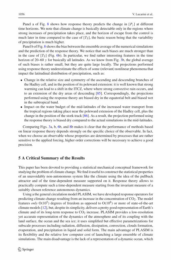
Panel a of Fig. 8 shows how response theory predicts the change in [Py] at differenttime horizons. We note that climate change is basically detectable only in the regions wherestrong increases of precipitation takes place, and the horizon of escape from the control ismuch later in time compared to the case of [TS], the basic reason being that the variabilityof precipitation is much higher.

Panel b of Fig. 8 shows the bias between the ensemble average of the numerical simulationsand the prediction of the response theory. We notice that such biases are much stronger thanin the case of [TS] (Fig. 6b). In particular, we find rather interesting features in the timehorizon of 20–60 y for basically all latitudes. As we know from Fig. 3b, the global averageof such biases is rather small, but they are quite large locally. The projections performedusing response theory underestimate the effects of some (relevant) nonlinear phenomena thatimpact the latitudinal distribution of precipitation, such as:

• Change in the relative size and symmetry of the ascending and descending branches ofthe Hadley cell, and in the position of its poleward extension: it is well known that strongwarming can lead to a shift in the ITCZ, where where strong convective rain occurs, andto an extension of the dry areas of descending [85]. Correspondingly, the projectionsperformed using the response theory are biased dry in the equatorial belt and biased wetin the subtropical band.

• Impact on the water budget of the mid-latitudes of the increased water transport fromthe tropical regions taking place near the poleward extension of the Hadley cell, plus thechange in the position of the stork track [86]. As a result, the projection performed usingthe response theory is biased dry compared to the actual simulations in the mid-latitudes.

Comparing Figs. 3a, b, 6b, and 8b makes it clear that the performance of methods basedon linear response theory depends strongly on the specific choice of the observable. In fact,when we choose an observable whose properties are determined by processes that are rathersensitive to the applied forcing, higher order corrections will be necessary to achieve a goodprecision.

5 A Critical Summary of the Results

This paper has been devoted to providing a statistical mechanical conceptual framework forstudying the problem of climate change.We find it useful to construct the statistical propertiesof an unavoidably non-autonomous system like the climate using the idea of the pullbackattractor and of the time-dependent measure supported on it. Response theory allows topractically compute such a time-dependent measure starting from the invariant measure of asuitably chosen reference autonomous dynamics.

Using a the general circulationmodel PLASIM, we have developed response operators forpredicting climate change resulting from an increase in the concentration of CO2. The modelfeatures only O(105) degrees of freedom as opposed to O(108) or more of state-of-the-artclimatemodels [12], but, despite its simplicity, delivers a pretty good representation of Earth’sclimate and of its long-term response to CO2 increase. PLASIM provides a low-resolutionyet accurate representation of the dynamics of the atmosphere and of its coupling with theland surface, the ocean and the sea ice; it uses simplified but effective parametrizations forsubscale processes including radiation, diffusion, dissipation, convection, clouds formation,evaporation, and precipitation in liquid and solid form. The main advantage of PLASIM isits flexibility and the relative low computer cost of launching a large ensemble of climatesimulations. The main disadvantage is the lack of a representation of a dynamic ocean, which

123


implies that we have a cut-off at the low frequencies, because we miss the multidecadal andcentennial variability due to the ocean dynamics. We have decided to consider classic IPCCscenarios of greenhouse forcing in order to make our results as relevant as possible in termsof practical implications.

The construction of the time dependent measure resulting from varying concentrations ofCO2 has been achieved by first performing a first set of simulations where N = 200 ensemblemembers sampled from a long control run undergo an instantaneous doubling of the initialCO2 concentration. Through simple numerical manipulations, we have been able to derivethe linear Green function for any observable of interest, which makes it possible to performpredictions of climate change to an arbitrary pattern of change of the CO2 concentrationusing simple convolutions, under the hypothesis that linearity is obeyed to a good degree ofapproximation.

We have studied the skill of the response theory in predicting the change in the globallyaveraged quantities as well as the spatial patterns of change to a forcing scenario of 1%per year increase of CO2 concentration up to doubling. We have focused on observablesdescribing the properties of two climatic quantities of great geophysical interest, namelythe surface temperature and the yearly total precipitation. The predictions of the responsetheory have been compared to the results of additional N = 200 direct numerical simulationsperformed according this second scenario of forcing.

The performance of response theory in predicting the change in the globally averagedsurface temperature and precipitation is rather good at all time horizons, with the predictedresponse falling within the ensemble variability of the direct simulations for all time horizonsexcept for a minor discrepancy in the time window 40–60 y. Additionally, our results confirmthe presence of a strong linear link in the form of modified Clausius–Clapeyron relationbetween changes in such quantities, as already discussed in the literature.

We have also studied how sensitive is the climate projection obtained using responsetheory to the size of the ensemble used for constructing the Green function. This is a matterof great practical relevance because it is extremely challenging to run a large number ofensemble members for specific scenarios using state-of-the-art climate models, given theirextreme computational cost [12]. We have then tested the skill of projections of globallyaveraged surface temperature and of globally averaged yearly total precipitation performedusing Green functions constructed using N = 20 ensemble members. We obtain that thequality of the projection is only moderately affected, and especially so in the case of thetemperature observable.

By performing convolution of the Green function with various scenarios where the CO2

increases at different rates, we are able to study the problem of climate change detection,associating to each rate of increase a time frame when climate change becomes statisticallysignificant. Another new aspect of climate response we are able to investigate thanks tothe methods developed here is the rigorous definition of transient climate sensitivity, whichbasically measures how different is the actual climate response with respect to the case ofquasi-adiabatic forcings, and defines the thermal inertia of climate.

Building upon the ideas proposed in [36], we have shown that response theory allows toput in a broader and well defined context concepts like climate sensitivity:

• we understand that the equilibrium climate sensitivity relates to the zero-frequencyresponse of the system to doubling of the CO2 concentration: it is then clear that if we arenot able to resolve the slowest time scales of the climate system, we will find so-calledstate-dependency [87,88] when estimating equilibrium climate sensitivity on slow (butnot ultraslow) time scales, because we sample different regions of the climatic attractor;

123


• we have that concepts like time-scale dependency [89] of the climate sensitivity are in factrelated to the concept of inertia of the climate response, which can be explored by gen-eralizing the idea of transient climate sensitivity [81] to all time scales of perturbations;

• in the case of coupled atmosphere-ocean models, looking at the transient climate sensi-tivity for different rates of CO2 concentration increase can be useful for understandingtheir multiscale properties.

The analysis of the spatial pattern of climate change signal using response theory is entirelynew and never attempted before. Clearly, when going from the global to local scale we haveto expect lower signal-to-noise ration, as the variability is enhanced, and the possibility thatlinearity is a worse approximation, as a result of powerful local nonlinear effects. Responsetheory provides an excellent tool also for predicting the change in the zonalmeanof the surfacetemperature, except for an underestimation of the warming in the very high latitude regionsin the time horizons of 40–60 y. This is, in fact, the reason for the small bias found alreadywhen looking at the prediction of the globally averaged surface temperature. By looking atthe 2D spatial patterns, we can associate such bias to a misrepresentation of the warming inthe region where the presence of sea-ice is most sensitive to changing temperature patterns.The fact that linear response theory has problems in capturing the local features of a stronglynonlinear phenomenon like ice-albedo feedback makes perfect sense. It is remarkable that,instead, response theory is able to predict accurately the change in the surface temperaturefields in most regions of the planet.

The prediction of the spatial patterns of change in the precipitation is much less successful,as a result of the complex nonlinear processes controlling the structure of the precipitativefield. In particular, response theory is not able to deal effectively with describing the polewardshift of the storm tracks, in the widening of the Hadley cell, and in the change of the ICTZ.

This paper provides a possibly convincing case for constructing climate change predictionsin comprehensive climate models using concepts and methods of nonequilibrium statisticalmechanics. The use of response theory potentially allows to reduce the need for runningmanydifferent scenarios of climate forcings as in [12], and to derive, instead, general tools for com-puting climate change to any scenario of forcings from few, selected runs of a climate model.Additionally, it is possible to deconstruct climate response to different sources of forcingsapart from increases in CO2 concentration, e.g. changes in CH4 and aerosols concentration,in land surface cover, in solar irradiance—and recombine it to construct very general climatechange scenarios. While this operation is easier in a linear regime, it is potentially doablealso in the nonlinear case, see [49] for details.

6 Challenges and Future Perspectives

The limitations of this paper point at some potentially fascinating scientific challenges to beundertaken. Let’s list some of them:

• A fundamental limitation of this study is the impossibility to resolve the centennialoceanic time scales. It is of crucial importance to test whether response theory is ableto deal with prediction on a wider range of temporal scales, as required when oceandynamics is included. We foresee future applications using a fully coupled yet efficientmodel like FAMOUS [90].

• One should perform a systematic investigation of how appropriate linear approximation isin describing climate response to forcings, by computing estimates of the Green function

123


using different level of CO2 increases and testing them against a wide range of timemodulating functions describing different scenarios of forcings.

• It is necessary to study in greater detail what is the minimum size of the ensemble neededfor achieving a good precision in the construction of the Green function; the requirementdepends on the specific choice of the observable, including how it is constructed in termsof spatial and temporal averages of the actual climatic fields.

• It is crucial to look at the effect of considering multiple classes of forcings in the climatechange scenarios and test how suitable combination of the individual Green functionsassociated to each separate forcing are able to predict climate response in general.

Different points of view on the problem of predicting climate response should as wellbe followed. The ab-initio construction of the linear response operator has proved elusivebecause of the difficulties associated with dealing effectively with both the unstable andstable directions in the tangent space. It is promising to try to approach the problem byusing the formalism of covariant Lyapunov vectors (CLVs) [91–94] for having a convincingrepresentation of the tangent space able to separate effectively and in an ordered manner thedynamics on the unstable and stable directions. CLVs have been recently shown to have greatpotential for studying instabilities and fluctuations in simple yet relevant geophysical systems[95]. By focusing on the contributions coming form the stable directions, one can also expectthat such an approach might allow for estimating the — otherwise hard to control — error inthe evaluation of the response operator introduced when applying the standard form of thefluctuation–dissipation theorem in the context of nonequilibrium systems possessing singularinvariant measure. This would help understanding under which conditions climate-relatedapplications of the fluctuation–dissipation theorem [17–21] have hope of being successful.

One of the disadvantages of the CLVs is that constructing them is rather demanding interms of computing power and requires a global (in time) analysis of the dynamics of thesystem, in order to ensure covariance, thus requiring relevant resources in terms of memory.Additionally, one expects that all the CLVs of index up to approximately the Kaplan–Yorkedimension of the attractor of the system are relevant for computing the response. Such anumber, albeit typically much lower than the number of degrees of freedom, can still beextremely large for an intermediate complexity or, a fortiori, in a comprehensive climatemodel.

At amore empirical level, a cheaper and effective alternativemay be provided by the use ofBred vectors (BVs). See comprehensive presentations in [96,97]. BVs are finite-amplitude,finite time vectors constructed as the difference between a background trajectory and a set ofperturbed trajectories, where the perturbations (initially chosen at random having a small, yetfinite norm) change following the nonlinear evolution of the trajectories, and are periodicallyrescaled to the prescribed initial norm. BVs provide a very efficient method for describing themain instabilities of the flow, taking into account nonlinear effects. In fact, what is extremelyinteresting about BVs is that (a) their growth factors are strongly dependent on the regionof the phase space where the system is; and (b) the choice of the reference norm of theperturbation and of the time interval between two successive renormalization procedures(breeding period) effects strongly the properties of the dominant instabilities specificallyactive on the chosen time scales. Clearly, in the limit of infinitesimally small reference normand infinitely long breeding time, all BVs converge to the first CLV. This is not the casewhen finite size effects become relevant. Instead, by considering not too small perturbationsand a long enough time interval, the very fast instabilitities associated to the first CLVs arewashed away by the loss of correlation due to nonlinear effects. In many applications ofmeteo-climatic relevance it has been shown that a relatively low number of BVs is extremely

123


effective for reconstructing the properties of the unstable space, and that BVs contain usefulinformation on spatially localized features, so that it may be worth trying to construct anapproximation to the Ruelle response operator using the BVs. One may note that consideringdifferent constructions of the BVs as discussed above might lead to the useful result ofunderlining different processes contributing to the response of the system.

Another promising approach for studying climate response relies on reconstructing theinvariant measure of the unperturbed system using its unstable periodic orbits (UPOs) [98].Unstable periodic orbits has been shown to be a useful tool for studying persistent patternsand transitions in the context of simple atmospheric models [99–101]. Since resonances inthe susceptibility describing the frequency-dependent response of specific observables canbe associated to dominating UPOs (compare, e.g., [37,102]), one can hope to be able toconstruct hierarchical approximations of the response operators by summing over larger andlarger set of UPOs.

Finally, it is worthmentioning that response theory can be approached in terms of studyingthe properties of the Perron–Frobenius transfer operator and of its generator [103] of theunperturbed and of perturbed system. In other terms, the focus is on studying directly howthe invariant measure changes as a result of the applied perturbation and the challenge is infinding appropriate mathematical embedding in terms of suitable functional spaces [43,104–106]. See [3] for a proposal going in the direction of studying climate change by lookingdirectly at measures rather than at observables, as instead done here.

While the practical application of such an approach in a very high-dimensional problemlike in the case of climate might in principle faces problems related to the curse of dimen-sionality, it has been advocated that it could provide an excellent framework for studyingvicinity of the climate to critical transitions [53], i.e. anticipating where there is no smooth-ness of the invariant measure with respect to perturbations. Such transitions are flagged bypresence of rough dependence of the system properties on the perturbation due to presenceof Ruelle–Pollicott resonances. This idea has been recently confirmed also analyzing longsimulations performed with PLASIM and constructing a reduced space from two carefullyselected observables [54].

Recently, a comprehensive response theory for Markov processes in a finite state spacehas been presented in the literature. Such a theory provides explicit matricial expressions ofstraightforward numerical implementation for constructing the linear and nonlinear responseoperators, including estimates of the radius of convergence [44]. Using such results in areduced state space might provide a novel and effective method for approaching the problemof climate response.

Acknowledgements The authors wish to thank M. Chekroun, H. Dijkstra, M. Ghil, A. Gritsun, A. vonder Heydt, and A. Tantet for sharing many ideas on climate sensitivity and climate response. Without suchstimulations this work would have hardly been possible. The authors want to thank M. Ghil for providing aconstructive and insightful review of this paper. VL wishes to thank D. Ruelle for sharing questions, answers,ideas, and doubts with such a special intellectual depth and generosity.

Open Access This article is distributed under the terms of the Creative Commons Attribution 4.0 Interna-tional License (http://creativecommons.org/licenses/by/4.0/), which permits unrestricted use, distribution, andreproduction in any medium, provided you give appropriate credit to the original author(s) and the source,provide a link to the Creative Commons license, and indicate if changes were made.

123

http://creativecommons.org/licenses/by/4.0/


References

1. Ghil,M.,Childress, S.: Topics inGeophysical FluidDynamics:AtmosphericDynamics,DynamoTheory,and Climate Dynamics. Springer, Heildelberg (1987)

2. Lucarini, V., Blender, R., Herbert, C., Ragone, F., Pascale, S., Wouters, J.: Mathematical and physicalideas for climate science. Rev. Geophys. 52(4), 809–859 (2014)

3. Ghil, M.: A mathematical theory of climate sensitivity or, how to deal with both anthropogenic forcingand natural variability? In: Chang, C.P., Ghil, M., Latif, M., Wallace, J.M. (eds.) Climate Change:Multidecadal and Beyond, pp. 31–51. Kluwer, Dordrecht (2015)

4. Ghil, M., Robertson, A.W.: “Waves” vs. “particles” in the atmospheres phase space: a pathway to long-range forecasting? Proc. Natl. Acad. Sci. USA 99, 2493–2500 (2002)

5. Lorenz, E.N.: The Nature and Theory of the General Circulation of the Atmosphere, vol. 218.TP.115.World Meteorological Organization, Geneva (1967)

6. Peixoto, J.P., Oort, A.H.: Physics of Climate. American Institute of Physics, New York (1992)7. Lucarini, V., Pascale, S.: Entropy production and coarse graining of the climate fields in a general

circulation model. Clim. Dyn. 43(3–4), 981–1000 (2014)8. Kleidon, A., Lorenz, R. (eds.): Non-equilibrium Thermodynamics and the Production of Entropy.

Springer, Berlin (2005)9. Lucarini, V.: Thermodynamic efficiency and entropy production in the climate system. Phys. Rev. E 80,

021118 (2009)10. Houghton, J. (ed.): IPCC Third Assessment Report: Working Group I Report, “The Physical Science

Basis”. Cambridge University Press, Cambridge (2001)11. Intergovernmental Panel on Climate Change: In: Solomon, S., et al. (eds.) The Physical Science Basis:

Working Group I Contribution to the Fourth Assessment Report of the IPCC. Cambridge UniversityPress, Cambridge (2007)

12. Intergovernmental Panel on Climate Change: In: Stocker, T., et al. (eds.) The Physical Science BasisIPCC Working Group I Contribution to AR5. Cambridge University Press, Cambridge (2013)

13. Allen, M.: Liability for climate change. Nature 421, 891–892 (2003)14. Hannart, A., Pearl, J., Otto, F.E.L., Naveau, P., Ghil, M.: Causal counterfactual theory for the attribution

of weather and climate-related events. Bull. Am. Meteorol. Soc. 97(1), 99–110 (2016)15. Lorenz, E.N.: Forced and free variations of weather and climate. J. Atmos. Sci 36, 1367–1376 (1979)16. Leith, C.E.: Climate response and fluctuation dissipation. J. Atmos. Sci. 32(10), 2022–2026 (1975)17. Langen, P.L., Alexeev, V.A.: Estimating 2× CO2 warming in an aquaplanet GCM using the fluctuation-

dissipation theorem. Geophys. Res. Lett. 32(23), L23708 (2005)18. Gritsun,A., Branstator, G.: Climate response using a three-dimensional operator based on the fluctuation-

dissipation theorem. J. Atmos. Sci. 64(7), 2558–2575 (2007)19. Abramov, R.V., Majda, A.: New approximations and tests of linear fluctuation-response for chaotic

nonlinear forced-dissipative dynamical systems. J. Nonlinear Sci. 18, 303–341 (2008). doi:10.1007/s00332-007-9011-9

20. Majda, A.J., Gritsun, A., Branstator, G.: Climate response of linear and quadratic functionals using thefluctuation-dissipation theorem. J. Atmos. Sci. 65, 28242841 (2008)

21. Cooper, F.C., Haynes, P.H.: Climate sensitivity via a nonparametric fluctuation-dissipation theorem. J.Atmos. Sci. 68(5), 937–953 (2011)

22. Ruelle, D.: A review of linear response theory for general differentiable dynamical systems. Nonlinearity22(4), 855–870 (2009)

23. Lucarini, V., Sarno, S.: A statistical mechanical approach for the computation of the climatic responseto general forcings. Nonlin. Proc. Geophys. 18, 7–28 (2011)

24. Franzke, C.L.E., O’Kane, T.J., Berner, J., Williams, P.D., Lucarini, V.: Stochastic climate theory andmodeling. Wiley Interdiscip. Rev. Clim. Change 6(1), 63–78 (2015)

25. Wouters, J., Lucarini, V.: Disentanglingmulti-level systems: averaging, correlations andmemory. J. Stat.Mech. Theory Exp. 2012(03), P03003 (2012)

26. Wouters, J., Lucarini, V.: Multi-level dynamical systems: connecting the ruelle response theory and theMori-Zwanzig approach. J. Stat. Phys. 151(5), 850–860 (2013)

27. Fraedrich, K., Jansen, H., Kirk, E., Luksch, U., Lunkeit, F.: The planet simulator: towards a user friendlymodel. Meteorol. Z. 14(3), 299–304 (2005)

28. Ghil, M., Chekroun, M.D., Simonnet, E.: Climate dynamics and fluid mechanics: natural variability andrelated uncertainties. Phys. D 237(1417), 2111–2126 (2008). Euler Equations: 250YearsOnProceedingsof an international conference

29. Chekroun, M.D., Simonnet, E., Ghil, M.: Stochastic climate dynamics: random attractors and time-dependent invariant measures. Phys. D 240(21), 1685–1700 (2011)

123

http://dx.doi.org/10.1007/s00332-007-9011-9

http://dx.doi.org/10.1007/s00332-007-9011-9


30. Carvalho, A.N., Langa, J., Robinson, J.C.: The pullback attractor. Attractors for Infinite-DimensionalNon-autonomous Dynamical Systems. Applied Mathematical Sciences, vol. 182, pp. 3–22. Springer,New York (2013)

31. Bódai, T.,Károlyi,Gy,Tél, T.:Achaotically drivenmodel climate: extremeevents and snapshot attractors.Nonlinear Process. Geophys. 18(5), 573–580 (2011)

32. Bódai, T., Tél, T.: Annual variability in a conceptual climate model: snapshot attractors, hysteresis inextreme events, and climate sensitivity. Chaos 22(2), 023110 (2012)

33. Bódai, T., Károlyi, G., Tél, T.: Driving a conceptual model climate by different processes: snapshotattractors and extreme events. Phys. Rev. E 87, 022822 (2013)

34. Drótos, G., Bódai, T., Tél, T.: Probabilistic concepts in a changing climate: a snapshot attractor picture.J. Clim. 28(8), 3275–3288 (2015)

35. Ruelle, D.: Nonequilibrium statistical mechanics near equilibrium: computing higher-order terms. Non-linearity 11(1), 5–18 (1998)

36. Ragone, F., Lucarini, V., Lunkeit, F.: A new framework for climate sensitivity and prediction: amodellingperspective. Clim. Dyn. 46, 1459–1471 (2016)

37. Lucarini, V.: Evidence of dispersion relations for the nonlinear response of the Lorenz 63 system. J. Stat.Phys. 134, 381–400 (2009). doi:10.1007/s10955-008-9675-z

38. Dijkstra, H.A., Ghil, M.: Low-frequency variability of the large-scale ocean circulation: a dynamicalsystems approach. Rev. Geophys. 43(3), RG3002 (2005)

39. Lucarini, V.: Modeling complexity: the case of climate science. In: Gähde, U., Hartmann, S., Wolf, J.H.(eds.) Models, Simulations, and the Reduction of Complexity, pp. 229–254. De Gruyter, Berlin (2013)

40. Saltzman, B.: Dynamical Paleoclimatology. Academic Press, New York (2001)41. Ruelle, D.: Thermodynamic Formalism. Addison-Wesley, Reading (1978)42. Gallavotti, G., Cohen, E.G.D.: Dynamical ensembles in stationary states. J. Stat. Phys. 80(5–6), 931–970

(1995)43. Baladi, V.: Linear response despite critical points. Nonlinearity 21(6), T81 (2008)44. Lucarini, V.: Response operators for Markov processes in a finite state space: radius of convergence and

link to the response theory for Axiom A systems. J. Stat. Phys. 162(2), 312–333 (2016)45. Lindenstrauss, J., Tzafriri, L.: Classical Banach Spaces. Springer, New York (1996)46. Ruelle, D.: A review of linear response theory for general differentiable dynamical systems. Nonlinearity

22, 855–870 (2009)47. Lucarini, V., Saarinen, J.J., Peiponen, K.-E., Vartiainen, E.M.: Kramers-Kronig Relations in Optical

Materials Research. Springer, New York (2005)48. Lucarini, V.: Response theory for equilibrium and non-equilibrium statistical mechanics: causality and

generalized kramers-kronig relations. J. Stat. Phys. 131, 543–558 (2008). doi:10.1007/s10955-008-9498-y

49. Lucarini, V., Colangeli, M.: Beyond the linear fluctuation-dissipation theorem: the role of causality. J.Stat. Mech. Theory Exp. 2012(05), P05013 (2012)

50. Abramov, R.V., Majda, A.J.: Blended response algorithms for linear fluctuation-dissipation for complexnonlinear dynamical systems. Nonlinearity 20(12), 2793–2821 (2007)

51. Eyink, G.L., Haine, T.W.N., Lea, D.J.: Ruelle’s linear response formula, ensemble adjoint schemes andlvy flights. Nonlinearity 17(5), 1867 (2004)

52. Wang, Q.: Forward and adjoint sensitivity computation of chaotic dynamical systems. J. Comput. Phys.235, 1–13 (2013)

53. Chekroun, M.D., Neelin, D.J., Kondrashov, D., McWilliams, J.C., Ghil, M.: Rough parameter depen-dence in climate models and the role of Ruelle-Pollicott resonances. Proc. Natl. Acad. Sci. USA 111(5),1684–1690 (2014)

54. Tantet, A., Lucarini, V., Lunkeit, F., Dijkstra, H.A.: Crisis of the chaotic attractor of a climate model: atransfer operator approach. ArXiv e-prints, July 2015

55. Lucarini,V., Fraedrich,K., Lunkeit, F.: Thermodynamic analysis of snowball earth hysteresis experiment:efficiency, entropy production, and irreversibility. Q. J. R. Met. Soc. 136, 2–11 (2010)

56. Boschi, R., Lucarini, V., Pascale, S.: Bistability of the climate around the habitable zone: a thermody-namic investigation. Icarus 226, 1724–1742 (2013)

57. Lucarini, V., Pascale, S., Boschi, V., Kirk, E., Iro, N.: Habitability andmultistability in earth-like planets.Astron. Nachr. 334(6), 576–588 (2013)

58. Held, I.M.: The gap between simulation and understanding in climate modeling. Bull. Am. Meteorol.Soc. 86(11), 1609–1614 (2005)

59. Fraedrich, K., Kirk, E., Lunkeit, F.: PUMA: Portable University Model of the Atmosphere. Technicalreport, Deutsches Klimarechenzentrum, Hamburg (1998)

123

http://dx.doi.org/10.1007/s10955-008-9675-z

http://dx.doi.org/10.1007/s10955-008-9498-y

http://dx.doi.org/10.1007/s10955-008-9498-y


60. Eliasen, E.,Machenhauer, B., Rasmussen, E.: On a numerical method for integration of the hydrodynam-ical equations with a spectral representation of the horizontal fields. Inst. of Theor. Met., KøbenhavnsUniversity, Copenhagen, Technical report (1970)

61. Orszag, S.A.: Transform method for the calculation of vector-coupled sums: application to the spectralform of the vorticity equation. J. Atmos. Sci. 27(6), 890–895 (1970)

62. Sasamori, Takashi: The radiative cooling calculation for application to general circulation experiments.J. Appl. Meteorol. 7(5), 721–729 (1968)

63. Lacis, A.A., Hansen, J.: A parameterization for the absorption of solar radiation in the earth’s atmosphere.J. Atmos. Sci. 31(1), 118–133 (1974)

64. Stephens, G.L., Paltridge, G.W., Platt, C.M.R.: Radiation profiles in extended water clouds. III: obser-vations. J. Atmos. Sci. 35(11), 2133–2141 (1978)

65. Stephens, G.L., Ackerman, S., Smith, E.A.: A shortwave parameterization revised to improve cloudabsorption. J. Atmos. Sci. 41(4), 687–690 (1984)

66. Slingo, A., Slingo, J.M.: Response of the National Center for Atmospheric Research community climatemodel to improvements in the representation of clouds. J. Geophys. Res. 96(D8), 15341 (1991)

67. Kuo, H.L.: On formations and intensification of tropical cyclone through latent heat release by cumulusconvection. J. Atmos. Sci. 22, 40–63 (1965)

68. Kuo, H.L.: Further studies of the parameterization of the influence of cumulus convection on large-scaleflow. J. Atmos. Sci. 31(5), 1232–1240 (1974)

69. Louis, J.F.: A parametric model of vertical eddy fluxes in the atmosphere. Bound. LayerMeteorol. 17(2),187–202 (1979)

70. Louis, J.F., Tiedke, M., Geleyn, M.: A short history of the PBL parameterisation at ECMWF. In: Pro-ceedings of the ECMWFWorkshop on Planetary Boundary Layer Parameterization, pp. 59–80. Reading(1981)

71. Laursen, L., Eliasen, E.: On the effects of the dampingmechanisms in an atmospheric general circulationmodel. Tellus 41A, 385–400 (1989)

72. Roeckner, E., Arpe, K., Bengtsson, L., Brinkop, S., Dümenil, L., Esch, M., Kirk, E., Lunkeit, F., Ponater,M., Rockel, B., Sausen, R., Schlese, U., Schubert, S., Windelband,M.: Simulation of present day climatewith the ECHAMmodel: impact ofmodel physics and resolution. Technical Report, 93. Technical report,Max Planck Institut für Meteorologie, Hamburg, 1992

73. Semtner, A.J.: A model for the thermodynamic growth of sea ice in numerical investigations of climate.J. Phys. Oceanogr. 6(3), 379–389 (1976)

74. Fasullo, J.T., Trenberth, K.E.: The annual cycle of the energy budget. part ii: meridional structures andpoleward transports. J. Clim. 21, 23132325 (2008)

75. Lucarini, V., Ragone, F.: Energetics of climate models: net energy balance and meridional enthalpytransport. Rev. Geophys. 49, RG1001 (2011)

76. Knietzsch, M.-A., Schröder, A., Lucarini, V., Lunkeit, F.: The impact of oceanic heat transport on theatmospheric circulation. Earth Syst. Dyn. 6(2), 591–615 (2015)

77. Fraedrich, K., Lunkeit, F.: Diagnosing the entropy budget of a climate model. Tellus A 60(5), 921–931(2008)

78. Lucarini, V., Fraedrich, K., Lunkeit, F.: Thermodynamics of climate change: generalized sensitivities.Atmos. Chem. Phys. 10, 9729–9737 (2010)

79. Liepert, B.G., Previdi, M.: Inter-model variability and biases of the global water cycle in CMIP3 coupledclimate models. Environ. Res. Lett. 7, 014006 (2012)

80. Liepert, B.G., Lo, F.: CMIP5 update of inter-model variability and biases of the global water cycle inCMIP3 coupled climate models. Environ. Res. Lett. 8, 029401 (2013)

81. Allen, M.R., Ingram, W.J.: Constraints on future changes in climate and the hydrologic cycle. Nature419(6903), 224–232 (2002)

82. Held, I.M., Soden, B.J.: Robust responses of the hydrological cycle to global warming. J. Clim. 19(21),5686–5699 (2006)

83. Pall, P., Allen, M.R., Stone, D.A.: Testing the Clausius-Clapeyron constraint on changes in extremeprecipitation under CO2 warming. Clim. Dyn. 28(4), 351–363 (2007)

84. O’Gorman, P.A.: Precipitation extremes under climate change. Curr. Clim. Change Rep. 1(2), 49–59(2015)

85. Chiang, J.C.H., Friedman, A.R.: Extratropical cooling, interhemispheric thermal gradients, and tropicalclimate change. Annu. Rev. Earth Planet. Sci. 40, 383–412 (2012)

86. Yin, J.H.: A consistent poleward shift of the storm tracks in simulations of 21st century climate. Geophys.Res. Lett. 32, L04704 (2005)

87. von der Heydt, A.S., Khler, P., van de Wal, R.S.W., Dijkstra, H.A.: On the state dependency of fastfeedback processes in (paleo) climate sensitivity. Geophys. Res. Lett. 41(18), 6484–6492 (2014)

123


88. Köhler, P., de Boer, B., von der Heydt, A.S., Stap, L.B., van de Wal, R.S.W.: On the state-dependency ofthe equilibrium climate sensitivity during the last 5 million years. Clim. Past Discuss. 11(4), 3019–3069(2015)

89. Senior, C.A., Mitchell, J.F.B.: The time-dependence of climate sensitivity. Geophys. Res. Lett. 27(17),2685–2688 (2000)

90. Jones, C., Gregory, J., Thorpe, R., Cox, P., Murphy, J., Sexton, D., Valdes, P.: Systematic optimisationand climate simulation of FAMOUS, a fast version of HadCM3. Clim. Dyn. 25, 189204 (2005)

91. Ginelli, F., Poggi, P., Turchi, A., Chaté, H., Livi, R., Politi, A.: Characterizing dynamics with covariantlyapunov vectors. Phys. Rev. Lett. 99, 130601 (2007)

92. Wolfe, C., Samuelson, R.M.: An efficientmethod for recovering Lyapunov vectors from singular vectors.Tellus A 59(3), 355–366 (2007)

93. Kuptsov, P.V., Parlitz, U.: Theory and computation of covariant Lyapunov vectors. J. Nonlinear Sci.22(5), 727–762 (2012)

94. Froyland, G., Hüls, T., Morriss, G.P., Watson, T.M.: Computing covariant Lyapunov vectors, Oseledetsvectors, and dichotomy projectors: a comparative numerical study. Phys. D 247, 18–39 (2013)

95. Schubert, S., Lucarini, V.: Covariant Lyapunov vectors of a quasi-geostrophic baroclinic model: analysisof instabilities and feedbacks. Q. J. R. Meteorol. Soc. 141(693), 3040–3055 (2015)

96. Deremble, B., D’Andrea, F., Ghil, M.: Fixed points, stable manifolds, weather regimes, and their pre-dictability. Chaos 19(4), 043109 (2009)

97. Norwood, A., Kalnay, E., Ide, K., Yang, S.-C., Wolfe, C.: Lyapunov, singular and bred vectors in amulti-scale system: an empirical exploration of vectors related to instabilities. J. Phys. A 46(25), 254021(2013)

98. Cvitanovíc, P., Eckhardt, B.: Periodic orbit expansions for classical smooth flows. J. Phys. Math. Gen.24, L237L241 (1991)

99. Selten, F.M., Branstator, G.: Preferred regime transition routes and evidence for an unstable periodicorbit in a baroclinic model. J. Atmos. Sci. 61(18), 2267–2282 (2004)

100. Gritsun, A.S.: Unstable periodic trajectories of a barotropic model of the atmosphere. Russ. J. Numer.Anal. Math. Modell. 23, 345–367 (2008)

101. Gritsun, A.S.: Statistical characteristics of barotropic atmospheric system and its unstable periodicsolutions. Dokl. Earth Sci. 435(2), 1688–1691 (2010)

102. Eckhardt, B., Ott, G.: Periodic orbit analysis of the lorenz attractor. Z. Phys. B 93(2), 259–266 (1994)103. Baladi, V.: Positive Transfer Operators and Decay of Correlations. World Scientific, Singapore (2000)104. Butterley, O., Liverani, C.: Smooth Anosov flows: correlation spectra and stability. J. Mod. Dyn. 1(2),

301–322 (2007)105. Liverani, C., Gouëzel, S.: Compact locally maximal hyperbolic sets for smooth maps: fine statistical

properties. J. Differ. Geom. 79, 433–477 (2008)106. Baladi, V.: Linear response, or else. ArXiv e-prints, August 2014

123

predicting climate change using response theory: global … · · 2017-04-11abstract the...

Documents