Predicting Bug-Fixing Time: An Empirical Study of Commercial Software Projects

Hongyu Zhang1, Liang Gong1, Steve Versteeg2, Jue Wang1, Zeqi Shen1, Janine Radford2 1Tsinghua University

Beijing 100084, China hongyu@tsinghua.edu.cn

2CA Technologies Melbourne, Australia

steve.versteeg@ca.com

Abstract—For a large and evolving software system, the project team could receive many bug reports over a long period of time. It is important to achieve a quantitative understanding of bug-fixing time. The ability to predict bug-fixing time can help a project team better estimate software maintenance efforts and better manage software projects. In this paper, we perform an empirical study of bug-fixing time for three CA Technologies projects. We propose a Markov-based method for predicting the number of bugs that will be fixed in future. For a given number of defects, we propose a method for estimating the total amount of time required to fix them based on the empirical distribution of bug-fixing time derived from historical data. For a given bug report, we can also construct a classification model to predict slow or quick fix (e.g., below or above a time threshold). We evaluate our methods using real maintenance data from three CA Technologies projects. The results show that the proposed methods are effective.

Index Terms—bugs, bug-fixing time, prediction, effort estimation, software mainteannce.

I. INTRODUCTION With the increasing complexity of software systems, the

task of quality assurance becomes more challenging. Modern enterprise software systems are typically composed of multiple components, each of which may have had a separate evolution. Furthermore, when deployed in the customer's environment, there are multiple environments and platforms to consider as well as the need for making complex interactions with third party systems. Therefore the organizations could receive a large number of bug reports over a long period of time. Fixing bugs is one of the most frequent software maintenance activities, which was estimated to cause 70 billion US dollars per year in the United States [17].

CA Technologies is a multinational company providing IT management software and solutions. Like other organizations, CA Technologies is committed to providing outstanding pre- and post-sales support for its customers. Bug fixing, as a part of software development and maintenance process, is an important activity of the company.

As the number of bugs reported by QA engineers and customers could be large, it is important to be able to predict the bug-fixing time so that a project team can better estimate the bug-fixing efforts and achieve better project management. We define the bug fix time as the calendar time from the creation of a bug record to the time the bug is resolved as fixed.

Although each bug is assigned with a severity and a priority, we find that we cannot simply predict bug-fixing time based merely on bug severity or priority. Bug-fixing time is affected by many other factors such as bug owners and bug types. Different bugs may require different amount of time to fix. The ability to estimate bug-fixing time is important for increasing customer satisfaction as well as for project planning. For example, a company may have a policy that all high severity bugs being fixed and at least P% of low severity bugs being fixed before releasing the product, the project team can then estimate how long it will take to fix the bugs to be compliant with the company’s policy. As another example, if a company has standards for responding customer reported issues, the project team can estimate if such standards can be met for a given bug report.

In recent years, there has been some research work on analyzing and predicting bug-fixing time. For example, Panjer [23] proposed to use classification techniques (such as Naïve Bayes) to predict the time to fix a bug. They obtained an accuracy of 34.9% on the Eclipse bug dataset. Kim et al. [13] studied the life span of bugs in ArgoUML and PostgreSQL projects, and found that bug-fixing time had a median of about 200 days. Giger et al. [9] studied three open source projects and used Decision Tree to classify fast and slowly fixed bugs. The aforementioned work only focuses on one aspect of bug-fixing time, and mainly on open source projects. Also, their prediction accuracy could be further improved.

In this paper, we perform a dedicated study on bug-fixing time using real data from three commercial projects of CA Technologies. We proposed methods for answering the following three questions: • How many bugs can be fixed? We propose a Markov

based method for predicting the number of bugs that can be fixed within a given time period. The evaluation results on three CA projects show that the mean relative error in prediction is only 3.72%.

• How much time is required to fix these bugs? We propose a Monte Carlo based method for predicting the total time required for fixing a given number of bugs. From the historical bug-fixing data, we can learn the empirical distribution of bug-fixing time, and utilize Monte Carlo simulations to estimate the total amount of time required for a project team to fix new bugs. The evaluation results

on three CA projects show that the mean relative error in prediction is only 6.45%.

• How long does it take to fix this bug? We confirm the previous work [9, 23] that we can predict the slow (e.g., above a time threshold) or quick (below a time threshold) fix for a certain bug by using the basic bug-related information collected from a bug-tracking system. We also propose a kNN-based method for classifying the bug-fixing time, which can improve the accuracy of existing methods. Our classification model utilizes basic bug-related features such as severity, priority, submitter, etc. We also define new distance metrics for measuring similarity between two bug reports, and apply the kNN technique to determine the effort required for a new bug based on the assumption that similar bugs require similar bug-fixing effort. The evaluations on three CA projects show that the overall F-measure is 72.45% on average.

For each of the above questions, we also show that the proposed methods outperform the existing methods, using the real data from CA.

We believe that our methods can help project teams improve the maintenance process and have the potential to be applied across companies. The rest of the paper is organized as follows. Section II briefly introduces the background about the bug-fixing process adopted at CA and an empirical study of a CA maintenance project. Section III presents the proposed method for predicting the number of fixed bugs. Section IV presents the proposed method for predicting the total time required for fixing a given number of bugs. Section V presents the proposed method for predicting whether it will be a slow or quick fix for an individual bug. Section VI describes our experimental design and Section VII presents the results. We discuss the proposed methods in Section VIII and threats to validity in Section IX. Section X briefly describes the related work and Section XI concludes this paper.

II. AN EMPIRICAL STUDY

A. The CA Maintenance Process CA Technologies defines many processes to ensure

software productivity and quality. The simplified bug-handling process adopted in CA is as follows. Once a bug is identified, it enters into the bug tracking system. The majority of bugs are found by QA, but some are raised by technical support in response to customer issues. New bugs are assigned to the development manager responsible for the release in which the bug was found. The submitter supplies information about the bug, to enable the developers to identify and resolve the issue.

Once a bug is created, the development manager examines the bug and verifies that the submission has been made correctly, i.e., all required information is present. If it is so, she/he assigns it to a developer to address the issue. The manager should also verify that the priority of the bug is set appropriately and correct it if necessary. The developer who is assigned the bug should examine the bug record and determines the problem. If the bug is not to be fixed in the current release, it is marked 'Deferred'. If the bug is fixed, the

developer submits the changes to source code repository and a QA will verify the bug fix. The development manager who is responsible for the release (to whom the bug was originally assigned when it was opened) will close the bug.

Submitted

Deferred Fixed

Closed

Figure 1. The simplified bug-handling process

B. An Empirical Study of a CA Maintenance Project To get a deeper understanding of the CA maintenance

process, we analyze an actual project (Project A) of CA Technologies and collect its maintenance data. This project relates to an IT management product for enterprise customers. The product has been released for more than five years and is used worldwide. Currently, approximately 60 developers, QA engineers and support engineers are involved in the maintenance of this project, implementing new feature requests and fixing bugs reported by the QA team and customers.

We perform an empirical analysis of the bug data of Project A. Not all bugs of Project A can be fixed quickly upon arrival, due to the limited resources, time constraints and unclear bug descriptions. We calculate the time needed to fix the bugs. Due to data sensitivity, only relative time scales are given, measured in “normalized units”, where 1 unit is approximately equal to the median time needed to fix a bug of Project A. We rank the bugs according to their fix time (in descending order, the bug with the longest fix time is ranked in the top).

0

5

10

15

20

25

0 1000 2000 3000 4000

Tim

e U

nits

Rank

Figure 2. The distribution of bug-fixing time for Project A

Figure 2 shows the distribution of bug-fixing time. Clearly, we can see that the time needed to fix the bugs exhibits large variations, ranging from near zero to 21 units. Furthermore, the effort distribution is an uneven, “long-tail” distribution - a large percentage of bugs are fixed within a relatively short time

period (e.g., within 1 time unit) and a small percentage of bugs require a long time to address. This analysis shows that the bug-fixing time is not uniformly or normally distributed, thus posing challenges for accurate prediction.

We also analyze the impact of different bug-related features on bug-fixing time. Table 1 shows the fixing time for bugs of different severities and priorities. In general, bugs with higher severity and priority are fixed faster (as indicted by the mean values). However, the variations (as indicated by the max and standard deviation values) of bug-fixing time are also large. There are no simple rules that can accurately estimate the bug-fixing time merely based on severity and priority. The problem of predicting bug-fixing time is not straightforward and requires further investigation.

Table 1. The fixing time (in units) for bugs of different severities and priorities

Feature Value Max Mean Std. Dev.

Severity Blocking 6.86 0.58 1.07 Functional 10.94 0.99 1.39 Enhancement 10.32 1.22 1.59 Cosmetic 10.06 1.24 1.73

Priority Critical 7.82 0.56 0.90 Serious 10.94 0.85 1.29 Medium 10.06 1.40 1.69 Minor 6.30 1.00 1.39

III. PREDICTING HOW MANY BUGS WILL BE FIXED We propose a method for predicting the number of bugs

that can be fixed by a given time in the future. Figure 3 shows the overall process of the method. We first construct a defect state transition model from the historical data. We then estimate the number of fixed bugs in the future based on the state transition model and the predicted total number of bugs.

HistoricalBug Data

SUBMITTEDFIXEDDEFERREDCLOSED

Analyzing Bug State Transitions

Constructing State Transition Models

Predicting Number ofFixed Bugs in the Future

Predicting Distribution of Bugs among States in the Future

Predicting Total Bug Numbers in the Future

0

1

2

3

4

5

6

Figure 3. The process of predicting the number of fixed bugs

In a defect state transition process such as the CA process shown in Figure 1, a bug’s next state is only dependent on its current state. Therefore, the state transition process can be treated as a Markov model (more specifically, the Discrete Time Markov Chain model). Figure 4 below describes the mapping from the CA defect state transition graph to a Markov model. In the mapping, each defect state is translated into a state labeled with a sequential number. Each arrow linking two

states has a transitional probability from the start state to the destination state. Moreover, for each state in the Markov model we add an arrow pointing to itself as a defect could remain in the same state at the next time interval. Such a defect transition model can represent the project team’s bug-fixing ability.

Submitted

Deferred Fixed

Closed

P1

P3 P2

P4

Figure 4. Mapping from CA defect handling process to a Markov

model

For the model shown in Figure 4, we can obtain the state transition probability matrix as follows:

𝑃𝑃 =

⎝

⎜⎜⎛

𝑝𝑝11𝑝𝑝12 … 𝑝𝑝1,𝑥𝑥−1𝑝𝑝1,𝑥𝑥𝑝𝑝21𝑝𝑝22 … 𝑝𝑝2,𝑥𝑥−1𝑝𝑝2,𝑥𝑥.

.

.𝑝𝑝𝑥𝑥,1𝑝𝑝𝑥𝑥,2 … 𝑝𝑝𝑥𝑥,𝑥𝑥−1 𝑝𝑝𝑥𝑥,𝑥𝑥⎠

⎟⎟⎞

where pij represents the probability from state i to state j, e.g. p12 represents the probability of a defect transferring from SUBMITTED to FIXED.

We gather statistics about the number of bugs in each state at an initial time t0, and then compute the distribution of bugs among the states (i.e., the state probability vector). We define the number of bugs in SUBMITTED, FIXED, DEFERRED and CLOSED as n1, n2, n3, and n4, respectively. Then the sum of the defects is S = 4

1 iin

=∑ , and the state probability vector at t0 is:

𝛼𝛼0 = (𝑛𝑛1𝑆𝑆� ,𝑛𝑛2

𝑆𝑆� ,𝑛𝑛3𝑆𝑆� ,𝑛𝑛4

𝑆𝑆� )

Utilizing the characteristic of Markov model [12], we can infer the distribution of bugs across the states at time t based on the initial states a0 and the state transition matrix P as follows:

𝛼𝛼𝑡𝑡 = 𝛼𝛼0 ∙ 𝑃𝑃𝑡𝑡

Assuming the number of fixed bugs at t is Nt, the number of bugs at the SUBMITTED state at time t is St, the number of newly submitted bugs between t and t +1 is ∆St+1, we can infer the number of bugs that can be fixed at time t+1 as follows:

𝑁𝑁𝑡𝑡+1 = 𝑁𝑁𝑡𝑡 + (𝑝𝑝12 + 𝑝𝑝13 ∙ 𝑝𝑝32 ) ∙ (𝑆𝑆 𝑡𝑡 + ∆𝑆𝑆 𝑡𝑡+1)

In the equation above, St, the number of bugs that remains at t, can be estimated using the following equations:

𝑆𝑆𝑡𝑡 = 𝑇𝑇𝑡𝑡 ∙ 𝛼𝛼𝑡𝑡𝑠𝑠𝑠𝑠𝑠𝑠𝑠𝑠𝑠𝑠𝑡𝑡𝑡𝑡𝑠𝑠𝑠𝑠 = 𝑇𝑇𝑡𝑡 ∙ (𝛼𝛼0 ∙ 𝑃𝑃𝑡𝑡)𝑠𝑠𝑠𝑠𝑠𝑠𝑠𝑠𝑠𝑠𝑡𝑡𝑡𝑡𝑠𝑠𝑠𝑠

∆𝑆𝑆 𝑡𝑡+1 = 𝑇𝑇𝑡𝑡+1 − 𝑇𝑇𝑡𝑡

, where Tt +1 and Tt are the total number of bugs at time t+1 and t, respectively. submitted

ta means the percentage of bugs at the SUBMITTED state at time t.

To estimate the Tt+1 value (the total number of bugs at time t+1), we apply regression analysis [22] to fit the growth curve of the bug numbers based on historical data, and then use the fitted regression model to predict the number of bugs at a future time.

IV. PREDICTING TOTAL BUG-FIXING TIME

In this section, we propose a Monte Carlo based method for predicting total time required for a project team to fix a given number of bugs. The process is shown in Figure 5. For a maintenance project, we first select the best-fitting distribution of bug-fixing time from the historical data. We then perform Monte Carlo simulations [6] over the selected distribution, and predict the total time required for fixing N new bugs.

HistoricalBug Data

Number of Bugs to be Fixed

Select the Best Fitting Distribution

Predicting Total Fixing Time via Monte Carlo Simulations

Analyze the Distributions of Bug-Fixing Time

0

1

2

3

4

5

6

0

1

2

3

4

5

6

0

1

2

3

4

5

6

Figure 5. The process of predicting time for fixing N bugs

An initial empirical study (as described in Section II) shows that the distribution of bug-fixing time is skewed. Some examples of commonly-found skewed distributions include exponential, lognormal and Weibull distributions. The details about these distributions can be found in statistics textbooks [25]. We should note that other skewed distributions could be also applied here to fit the actual data about bug-fixing time.

To determine the best-fitting distribution function P, we evaluate the goodness of the fitting using the coefficient of determination (R2) and the Standard Error of Estimate (Se) [22]. The R2 statistic measures the percentage of variations that can be explained by the model. Its value is between 0 and 1, with higher value indicating a better fit. Se is a measure of the absolute prediction error and is computed as:

2)'( 2

−

−= ∑

nyy

Se

, where y and y’ are the actual and predicted values, respectively. The larger Se indicates the larger prediction error.

After determining the statistical distribution function P that best fits the historical bug-fixing data, we can then estimate the total time for fixing N new bugs using Monte Carlo simulations. Monte Carlo simulation [6] is a statistical simulation that uses repeated random sampling to compute results. It has been

widely applied to solve problems in many fields such as physics, finance, and engineering.

To estimate the time required for fixing N bugs, we randomly sample N numbers from the distribution of bug-fixing time P, using the parameters obtained from the historical data. These N numbers are pseudo random numbers that follow the same distribution as P. Each number represents bug-fixing time for a bug. We then compute the sum of these N numbers. We perform such a simulation process many times (e.g., 100 times) and calculate the average value as the final prediction output.

V. PREDICTING FXING TIME OF INDIVIDUAL BUGS In this section we propose a method for predicting

slow/quick fixes. The “slowness”/“quickness” is defined by a threshold such as 1 or 2 time units. We first identify the features of bugs and compute the similarities between bug reports. We then construct a kNN-based classification model for predicting for a given bug report whether the fix will be slow or quick, based on the assumption that the similar bugs could require similar bug-fixing effort.

A. Feature Collection We are able to collect the following bug-related features

from the CA bug tracking system to construct the prediction model: • Submitter: the bug report submitter. • Owner: the developer who is responsible for resolving the

bug • Severity: the severity of a bug report (Blocking,

Functional, Enhancement, Cosmetic, or Request for Information).

• Priority: the priority of a bug report (Critical, Serious, Medium, Minor)

• ESC: indicating whether the bug is an externally discovered bug (reported by end users) or an internally discovered bug (reported by the QA team).

• Category: the category of the problem (such as Account Management, Documentation, Configuration, etc.). The existing bug tracking system used in CA predefines a list of categories, and allows the users to manually select which category the bug belongs to.

• Summary: a short description of the problem.

For the bug Priority and Severity features, we define metrics to capture their data characteristics and use the measurement values as input to the classification model (Section V.B). For the bug Summary feature, we compute the distance between two summaries by comparing the words contained (Section V.C).

B. Measuring Distance in Priorities and Severities There are four levels of priorities in the CA projects:

“Critical”, “Serious”, “Medium”, “Minor”. Conventionally, an instance-based classifier such as kNN calculates the distance between non-numeric values using the following formula:

1 21 2

1 2

1( , )

0v v

d v vv v≠

= =

As d(Critical, Serious) should be smaller than d(Critical, Minor), we define the distances between different priorities as shown in Figure 6. For example, the distance between Critical and Minor bugs is 0.75, and the distance between Critical and Medium bugs is 0.5. This distance measure is used when computing the distances between bug reports of different priorities. In the same manner, we also define distances between different severities.

Critical

Serious

Medium

Minor

0.5

0.50.25

0.25

0.25

0.75

Figure 6. Measuring the distances between bug priorities

C. Measuring Distance in Bug Summary Many bug tracking systems, including the one used in CA

Technologies, contain a summary for each bug report describing the symptoms of the problem. To measure the distance between the summaries of two bug reports, we use the bag of words model [15] and calculate the distance ( , )Sd α β between bug reports α and β by considering how different the two sets of words are.

To eliminate useless words like “or”, “that”, “in”, or “contains”, we first generate a set of standard words extracted from the CA pre-defined categories. When comparing the difference between two sets of words from bug’s reports, we only count those contained in the standard word set.

( ) ( )( , ) 1

( ) ( ) 1C

SC

W S W S Wd

W S W S Wα β

α β

α β = −+

, where Sα stands for the synopsis of α and ( )W Sαrepresents

the set of words appeared. CW is the set of standard words

extracted from pre-defined category labels.

D. Construction of Classificaiton Model We use an adapted kNN (k-Nearest Neighbor) classifier in

our method, based on the assumption that a new bug should belong to the class of its similar bugs. kNN is a typical instance-based learning classifier. To measure the distance between two bug repots, we define the following Euclidean based distance metric:

2 2

1( , ) ( , ) ( , )

fN

R S i ii

d d dα β α β α β=

= +∑

, where α and β are two different bug reports.f

N counts the

total number of features, and i

α represents the i-th feature value of bug α . ( , )i id α β represents the Euclidean distance in the ith feature between bugs α and β . ( , )Sd α β represents the distance between the summaries of the two bugs.

After constructing the kNN-based classification model, we then predict whether the fix will be slow or quick (exceed or below a certain time threshold) for a new bug report.

VI. EXPERIMENTAL DESIGN

A. Datasets To evaluate the proposed methods, we use bug datasets

collected from three CA Technologies projects. Project A is the project we described in Section II. Projects B and C are for other commercial IT management products released by CA. All these projects have actively maintained the associated products for at least 5 years. We analyze the bugs reported over a 45 month interval for Project A, a 30 month interval for Project B, and a 29 month interval for Project C. The bugs are found by the QA teams and customers. Due to sensitivity, we cannot release the actual number of reported and fixed bugs during these periods. All these projects are large-scale projects which involve 40-100 developers, QA engineers, and support engineers.

B. Research Questions In this section, we evaluate the effectiveness of the

proposed methods for predicting the bug-fixing time. We design the experiments to answer the following research questions:

RQ1: How many bugs can be fixed?

In this RQ, we evaluate the ability of the proposed method for predicting the number of bugs that can be fixed within a given time period in the future. To do this, we train a prediction model using 12 months of data and then predict the number of bugs which can be fixed in three months immediately following the training time period.

To further evaluate the effectiveness of the proposed method, we compare it with a simple prediction method (average-based method) that uses the average number of fixed bugs in the past to predict the number fixed bugs in the next M months:

0mN N M x= + × , where N0 and Nm represent the number of fixed bugs at time t0 and tm, respectively. x is the arithmetic average of fixed bugs in each month obtained from the training data.

To evaluate the accuracy of the predictions, we use the MRE (Magnitude Relative Error) metric, which is defined as follows:

| - ' |y yMREy

=

, where y and y’ are the actual value and its estimate, respectively. The value of MRE is between 0 and 1. The smaller the value shows the better the estimation will be.

RQ2: How accurate is the proposed method for predicting the time for fixing N bugs?

In this RQ, we evaluate the ability of the proposed Monte Carlo based method for predicting the total amount of time required for fixing a given number of bugs. To do this, for each studied project, we randomly sample 90% of the maintenance data as the training set and obtain the best-fit statistical distribution of bug-fixing time. We then perform Monte Carlo simulations to obtain the bug-fixing time for the rest of 10% data. The Monte Carlo simulation is performed using the MATLAB tool. We then compare the predicted and actual results using the MRE metric.

We also compare the proposed method with an average-based method, which is a simple prediction method that uses the arithmetic average of bug-fixing time (x ) obtained from the training data to predict the time required to fix N bugs in the test data.

xNy ×= As there is currently lack of related methods for

predicting the total time required for fixing bugs, we expect that the proposed method should at least outperform the simple average-based method.

RQ3: How accurate is the proposed method for predicting fixing time for an individual bug?

In this RQ, we evaluate the ability of the proposed kNN-based method for predicting slow/quick fix for a given bug. We use different thresholds to determine slow-to-fix bugs (0.1, 0.2, 0.4, 1, and 2 time units), and examine the performance of the proposed method.

In this RQ, we also evaluate if the proposed method is more effective than the existing methods [9, 23]. The existing methods use basic bug-related information without improvement (without introducing new distance measures), and adopt commonly-used classifiers including Decision Tree and Naïve Bayes. Furthermore, we also compare with other classifiers such as Bayesian Network (BayesNet) and RBF Network. In our experiments, we use the implementations of these classifiers in WEKA [29], an open source data mining tool.

To evaluate the performance of the proposed approach in predicting the time to fix a bug, we adopt the commonly-used metric weighted average F-measure [29]. F-measure considers both Recall and Precision to score the accuracy. For each class (e.g., CQ for quickly fixed bugs and CS for slowly fixed bugs), the F-measure with respect to a particular class Ci is defined as follows:

2 i i

i

i i

C CC

C C

precision recallF

precision recall

⋅= ⋅

+ The weighted F-measure calculates the weighted average F-

measure considering the class size: 1

i i

ii

i

C CCC

C

F N FN

= ⋅ ⋅∑∑

, where iCN is the total number of bugs whose actual labels are

Ci in the testing set. The values of weighted average F-measure are between 0 and 1, the higher the better.

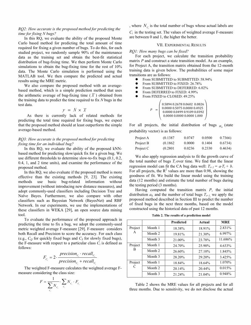
VII. EXPERIMENTAL RESULTS RQ1: How many bugs can be fixed?

For each project, we calculate the transition probability matrix P and construct a state transition model. As an example, for Project A, the transition matrix obtained from the 12-month training data is given below. The probabilities of some major transitions are as follows: From SUBMITTED to SUBMITTED: 58.94% From SUBMITTED to FIXED: 26.78% From SUBMITTED to DEFERRED: 6.02% From DEFERRED to FIXED: 4.99% From FIXED to CLOSED: 49.25%

𝑃𝑃 =

⎝

⎜⎜⎛

0.5894 0.2678 0.0602 0.0826 0.0000 0.5075 0.0000 0.4925 0.0000 0.0499 0.9109 0.03920.0000 0.0000 0.0000 1.000

⎠

⎟⎟⎞

For all projects, the initial distribution of bugs 0α (state

probability vector) is as follows: Project A (0.1387 0.0747 0.0500 0.7366) Project B (0.1862 0.0000 0.1404 0.6734) Project C (0.2801 0.0236 0.2330 0.4634)

We also apply regression analysis to fit the growth curve of the total number of bugs Tt over time. We find that the linear regression model can fit the CA bug data well: Tt+1 = a⋅Tt + b. For all projects, the R2 values are more than 0.98, showing the goodness of fit. We build the linear model using the training data (12 months) and estimate the total number of bugs during the testing period (3 months).

Having computed the transition matrix P, the initial distribution a0, and the number of total bugs Tt+1, we apply the proposed method described in Section III to predict the number of fixed bugs in the next three months, based on the model constructed using the historical data of past 12 months.

Table 2. The results of a prediction model

Predicted Actual MRE Project

A Month 1 18.38% 18.91% 2.831% Month 2 19.81% 21.30% 6.997% Month 3 21.00% 23.78% 11.686%

Project B

Month 1 24.70% 25.90% 4.633% Month 2 26.60% 27.10% 1.845% Month 3 28.20% 29.20% 3.425%

Project C

Month 1 18.84% 18.64% 1.070% Month 2 20.14% 20.44% 0.015% Month 3 21.24% 21.04% 0.948%

Table 2 shows the MRE values for all projects and for all

three months. Due to sensitivity, we do not disclose the actual

and predicted number of fixed bugs. Instead, we use the percentage values (with respect to the total number of bugs) to denote them. For example, for Project A, our method predicts that there are 18.38% fixed bugs in Month 1, while the actual number is 18.91%. The MRE value is only 2.831%. For all predictions, MRE values range from 0.015% to 11.686%, with an average of 3.72%. The results show that the predictions are accurate and consistent across all months and across all projects.

Our experiments also show that the proposed method outperforms the average-based method. For example, Figure 7 shows the comparison results in MRE for Project A. The improvement over the average-based method ranges from 10% to 44%.

0.00%

2.00%

4.00%

6.00%

8.00%

10.00%

12.00%

14.00%

Month 1 Month 2 Month 3

MRE Proposed

Average-based

Figure 7. The comparisons between the proposed method with the

average-based method (Project A)

RQ2: How accurate is the proposed method for predicting fixing time of N bugs?

For each studied project, we first select the best-fitting empirical distribution of bug-fixing time from the training set. We evaluate three distributions: Weibull, lognormal, and exponential distributions using the R2 value and Se values, and then determine the best distribution. The results are shown in Table 3. We can see that the Weibull distribution is the best-fitting distribution for Project A, and the Lognormal distribution is the best for Projects B and C.

These results can be also visually represented in the form of CDF (Cumulative Distribution Function). For example, Figure 8 shows the CDFs we obtained for Project A, which confirms that the distribution of bug-fixing time can be best modeled using a Weibull function.

Table 3. The distributions of bug-fixing time

Distribution R2 Se Project A Exponential 0.9229 0.0438

Lognormal 0.9879 0.0159 Weibull 0.9933 0.0128

Project B Exponential 0.4972 0.082 Lognormal 0.98 0.0163

Weibull 0.9578 0.0238 Project C Exponential 0.8482 0.0639

Lognormal 0.9868 0.0188 Weibull 0.9776 0.0246

Figure 8. The distributions of bug-fixing time (Project A)

After obtaining the empirical distributions of bug-fixing time from the training set (90% of the data), we can then apply the proposed method as described in Section IV to predict the time required for fixing the bugs in the test set (10% of the data). We choose the best-fitting distribution for each project and run Monte Carlo simulations to obtain the total bug-fixing time. The experiments are repeated 100 times and the average is computed. The results are shown in Figure 9. For the three projects, the MRE values are low (between 1.04% and 15.76%, with an average of 6.45%), confirming the usefulness of the proposed method. Figure 9 also shows that the proposed method outperforms the average-based method. The relative improvement ranges from 38.5% to 67.1%.

0.00%

5.00%

10.00%

15.00%

20.00%

25.00%

30.00%

35.00%

Project A Project B Project C

MRE Proposed

Average-based

Figure 9. The results for predicting bug-fixing time

RQ3: How accurate is the proposed method for predicting fixing time for an individual bug?

Table 4 shows the evaluation results (in terms of weighted F-measure) for predicting fixing time for each individual bug, under different time thresholds δ (0.1, 0.2, 0.4, 1, and 2 time units). In general, all classifiers can lead to weighted F-measure above 60%. Our results confirm the existing work [9, 23], that using classification techniques (such as Naïve Bayes), we can predict whether a bug will be fixed slowly or quickly based on the basic bug-related information collected from a bug-tracking system.

Table 4 also shows that in general the proposed method outperforms the related methods. For example, for predicting if the fixing time for a given bug in Project A is below or above 0.4 time unit, using the proposed prediction model we could

achieve the weighted F-measure 66.8%, which is higher than the results obtained from other methods. In general, for all projects and all thresholds, the weighted F-measure obtained from the proposed method ranges from 65% to 85% (with an average of 72.45%). The results confirm the effectiveness of the new distance metrics introduced in the proposed method. We also conduct Pair-wised Wilcoxon Test, and the results show that the proposed approach statistically outperforms other classifiers at 99% confidence interval. Table 4. The results for predicting slow or quick fix of a bug (F-measure)

δ 0.1 0.2 0.4 1 2

Project A

Proposed 0.704 0.659 0.668 0.728 0.852 BayesNet 0.702 0.633 0.638 0.704 0.828 Naïve Bayes 0.701 0.636 0.638 0.698 0.832 RBFNetwork 0.691 0.631 0.630 0.696 0.833 Decision Tree 0.653 0.495 0.643 0.601 0.798

Project B

Proposed 0.679 0.685 0.650 0.672 0.703

BayesNet 0.669 0.613 0.597 0.637 0.643

Naïve Bayes 0.670 0.610 0.605 0.642 0.645

RBFNetwork 0.679 0.614 0.610 0.621 0.628

Decision Tree 0.618 0.520 0.627 0.670 0.632

Project C

Proposed 0.770 0.793 0.762 0.769 0.773

BayesNet 0.787 0.768 0.722 0.745 0.78 Naïve Bayes 0.790 0.773 0.739 0.745 0.775 RBFNetwork 0.784 0.780 0.739 0.741 0.75

Decision Tree 0.662 0.776 0.741 0.740 0.765

To further confirm the superiority of the proposed method, we compare the effectiveness of two predicting methods PA and PB by using one of the methods (for example, PB) as reference measure. When using the same training set and testing set, the predicting accuracy difference: Metric(PA) - Metric(PB) is considered as the improvement of PA over PB. A positive value means that PA performs better than PB (since higher accuracy is better). The difference corresponds to the magnitude of improvement. For example, if the F-measure from PA is 70% and the F-measure of PB is 60%, then the improvement of PA over PB is 10%.

For the studied projects, we run the prediction 200 times, and check the improvement of the proposed method over the other methods at each time. We find that the proposed method outperforms the other methods most of the times. For example, Figures 10 and 11 show the improvement of the proposed approach (PA) over RBFNetwork (PB) and Decision Tree (PB), respectively (when the threshold is 0.6 time unit). The results show that the proposed method outperforms the other classifiers in most cases. The improvements over RBFNetwork are between 0.05% and 9.46%. The improvements over Decision Tree are between 10.35% and 31.78%. The results confirm the superiority of the proposed method.

-0.06

-0.04

-0.02

0

0.02

0.04

0.06

0.08

0.1

0.12

1 21 41 61 81 101 121 141 161 181

Impr

ovem

ents

No. of Times

Figure 10: Improvement of the proposed method over RBFNetwork on Project A

0

0.05

0.1

0.15

0.2

0.25

0.3

0.35

1 21 41 61 81 101 121 141 161 181

Impr

ovem

ents

No. of Times

Figure 11: Improvement of the proposed method over Decision Tree on Project A

VIII. DISCUSSIONS

A. Which Features are More Effective? It is known that different features could have different

impact on bug-fixing time. For example, Panjer [23] found that the most influential factors affecting bug lifetime are commenting activity, bug severity, component, and version. Guo et al. [10] performed an empirical study to characterize factors that affect which bugs get fixed in Windows Vista and Windows 7. They found that bugs reported by people with better reputations were more likely to be fixed. Bhattacharya and Neamtiu [3] performed multivariate and univariate regression testing on some open source projects and reported there is no correlation between bug-fix likelihood, bug-opener’s reputation and the time it takes to fix a bug.

In this study, we analyze the impact of each feature on predicting bug-fixing time for each individual bug. We use three commonly-used feature ranking methods, namely Chi-square, Gain Ratio and Information Gain [29]. The results are shown in Figure 12. All three feature ranking methods show that the Submitter and Owner are the top 2 most important features, which contribute 17% to 31% of the classification results. Our results confirm what Guo et al. [10] obtained from the experiments on the Windows projects.

0%

5%

10%

15%

20%

25%

30%

35%

Priority Severity Submitter Owner Category Esc

Impo

rtan

ce

Features

Chi-square

Gain Ratio

Info Gain

Figure 12. The contribution of different features evaluated by three

feature ranking metrics

B. Why Sometimes the Prediction is Wrong? Our experiments show that the proposed method is

effective in predicting bug-fixing time. However, it is not perfect and could still lead to prediction errors. To analyze why some bug reports’ fixing time cannot be accurately predicted, we take a look at some incorrectly classified bugs in detail. For example, for the bug (#101209), most of its neighbors suggest that this bug could be fixed quickly. However, actually this bug took much longer time to fix. The nearest neighbor of the bug #101209 is the bug #110284. These two bugs share the same priority, severity, submitter, owner, and problem category. However, they required different amount of time to fix. In this study, we collected the features from the CA bug tracking system. This example shows that merely considering the existing features are not always sufficient for differentiating bug-fixing time. There could have more features (such as the organizational and geographical distances [10] and developer behavior [24]) affecting the bug-fixing time. Identifying these features could help further improve the prediction accuracy. This remains an important future work.

IX. THREATS TO VALIDITY We have identified some threats to validities that should be

taken into consideration when applying the proposed method: • Large evolving system: The method we proposed is

suitable for large software systems that are experiencing a long period of evolution and their project team’s bug-fixing performances are stable. For a small or short-lived system, the number of bugs and state transitions are often small, thus making the statistical analysis inappropriate.

• Industry data: All datasets used in our experiments are collected from the actual maintenance projects of CA. The defect handling process of open source projects may be different from that of commercial projects. We will evaluate if the proposed methods can be applied to a variety of projects including open source projects. This is an important consideration for future work.

• Limited information: In this study, we use readily available bug-related information provided by the existing bug tracking system. This information could be limited.

Identifying and collecting more information could further improve the prediction results.

X. RELATED WORK In recent years, there have been many empirical studies on

software defects. For example, software defect prediction methods collect historical defect data by mining software repositories (such as bug database and version archives), identify program features (such as complexity and process metrics), and then build classification models to predict the defect-proneness (defective or non-defective) of a new module [19, 27]. There are also studies on the empirical analysis of defect distributions in a large software project [1, 7]. Some researchers also studied defect life cycles [16, 30] and triage [2, 11]. In this work, we perform an empirical study of the bug-fixing time using real industrial, and proposed methods to predict the effort required to fix bugs.

In software engineering, estimation techniques such as COCOMO [4] were propose to estimate software development efforts based on project size (measured in terms of lines of code or function points) and technical complexity factors. COQUALMO (COnstructive QUALity MOdel) [5] is an estimation model that can be used for predicting number of residual defects/KSLOC (Thousands of Source Lines of Code) or defects/FP (Function Point) in a software project. It could analyze the impact of various defect removal techniques and the effects of personnel and project characteristics on software quality. However, these techniques cannot be directly applied to estimate bug-fixing time.

There are also studies on the measurement of bug-fixing performance. For example, Mockus et al. proposed quality metrics (such as percentage of defective files) to understand software maintenance effort quantitatively [8, 20]. Mockus also proposed regression models to estimate maintenance effort and its distribution over time [21]. Kim et al. [13] studied the life span of bugs in ArgoUML and PostgreSQL projects, and found that bug-fixing time has a median of about 200 days. Guo et al. [10] performed an empirical study to characterize factors that determine which bugs get fixed in Windows 7. They found that bugs reported by people with higher reputation were more likely to get fixed, as were bugs opened by people on the same development team and working in geographical proximity.

Some researchers also proposed methods for predicting bug-fixing efforts. For example, Panjer [23] proposed to use machine-learning models to predict the time to fix a defect. Zeng and Rine [31] propose to predict the bug-fix effort using Neural Networks on a NASA dataset. Using a Random Forest algorithm, Marks et al. [18] can correctly predict the class (low or high fix effort) of a bug fix with a success rate of 65%. Song [26] proposed association rule based methods for predicting bug associations and bug-fixing effort. Weiß et al. [28] studied the lifecycle of bugs and proposed to use kNN method to determine the fix-effort for bugs in the JBoss project. In our work, we propose a kNN-based method for predicting fixing time for a bug. We also introduce new distance metrics for comparing the similarity between two bug reports, which can improve the prediction accuracy.

XI. CONCLUSIONS Bug fixing is an important activity for almost all software

organizations. The ability to predict bug-fixing time can help estimate maintenance effort and improve project management. Based on empirical studies of three CA maintenance projects, we have proposed the following methods: • a Markov model based method for predicting the number

of fixed bugs in the future. The evaluation results show that the mean relative error in prediction is only 3.72%.

• a Monte Carlo based method for predicting the total time required for fixing a given number of bugs. The evaluation results show that the mean relative error in prediction is only 6.45%.

• a kNN-based method for classifying the time (slow or quick) required for fixing a certain bug. The evaluation results show that we can achieve an average weighted F-measure 72.45%.

We believe that our methods have a potential to be applied to other software organizations to improve their software maintenance process. For example, if an organization’s QA policy requires that at least P% of bugs being fixed before releasing a product, then our methods can estimate how long it would take to fix these bugs and the associated cost. Our method could also estimate the number of bugs that can be fixed within a given future time period, and predict the slow or quick fix of a given bug.

In the future, we plan to carry out large-scale evaluations of the proposed method on a variety of projects. We will also identify more factors (including project, developer and organization related factors) that could affect the bug-fixing time and analyze the causal relationships among them.

ACKNOWLEDGEMENT This research is supported by a CA Labs research

collaboration grant, and partially by a NSFC grant 61073006. We thank many CA developers for their helpful discussions on the CA development and maintenance processes.

REFERENCES [1] C. Andersson and P. Runeson, A Replicated Quantitative

Analysis of Fault Distributions in Complex Software Systems, IEEE Trans. Software Eng., 33 (5), pp. 273-286, May 2007.

[2] J. Anvik, L. Hiew, and G. C. Murphy. Who should fix this bug? In Proc. ICSE 2006, pages 361–370, ACM, 2006.

[3] P. Bhattacharya, I. Neamtiu: Bug-fix time prediction models: can we do better?, Proc. MSR 2011, 207-210, 2011.

[4] B. Boehm, Software Engineering Economics, Prentice-Hall, 1981.

[5] COQUALMO: http://csse.usc.edu/csse/research/COQUALMO/ [6] L. Devroye, Non-Uniform Random Variate Generation, New

York: Springer-Verlag, 1986. [7] N. Fenton and N. Ohlsson, Quantitative Analysis of Faults and

Failures in a Complex Software System, IEEE Trans. Software Eng., 26 (8), Aug 2000. pp. 797-814.

[8] D. German, A. Mockus, Automating the measurement of open source projects, ICSE '03 Workshop on Open Source Software Engineering, Portland, Oregon, May 2003.

[9] E. Giger, M. Pinzger, and H. Gall, Predicting the fix time of bugs. In Proc. RSSE '10, pp.52-56, 2010.

[10] P. J. Guo, T. Zimmermann, N. Nagappan, and B. Murphy. Characterizing and predicting which bugs get fixed: An empirical study of Microsoft Windows. In Proc. ICSE’10, May 2010.

[11] P. J. Guo, T. Zimmermann, N. Nagappan, B. Murphy: "Not my bug!" and other reasons for software bug report reassignments. In Proc. CSCW 2011, pp. 395-404, 2011.

[12] E. Kao, An Introducation to Stochastic Processes, Duxbury Press, 1996.

[13] S. Kim and J. E. James Whitehead. How long did it take tofix bugs? In MSR ’06, pp. 173–174, May 2006.

[14] S. Kim, et al., Classifying Software Changes: Clean or Buggy?, IEEE Trans. on Software Engineering, vol. 34, pp. 181-196, March/April 2008.

[15] Y. Ko. A study of term weighting schemes using class information for text classification. In Proc. SIGIR, pp.1029-1030. 2012.

[16] T. Koponen, Life cycle of Defects in Open Source Software Projects, IFIP International Federation for Information Processing, 2006, pp.195-200

[17] M. Lerner, Software maintenance crisis resolution, the new IEEE standard, IEEE Softw. Devel (Aug.), 65-72, 1994.

[18] L. Marks, Y. Zou, and A. E. Hassan, Studying the fix-time for bugs in large open source projects. In Proc. PROMISE '11. 2011.

[19] T. Menzies, J. Greenwald, and A. Frank. Data mining static code attributes to learn defect predictors. IEEE Trans. Softw.Eng., 33(1): 2–13, 2007.

[20] A. Mockus, R. T. Fielding, and J. D. Herbsleb. Two case studies of open source software development: Apache and Mozilla. ACM Trans. Softw. Eng. Methodol., 11(3):309–346, 2002.

[21] A. Mockus, D. M. Weiss, and P. Zhang. Understanding and predicting effort in software projects. In Proc. ICSE 2003, pp. 274–284, Portland, Oregon, May 2003.

[22] J. D. Musa, Software Reliability: Measurement, Prediction and Application, McGraw-Hill, New York, 1987.

[23] L. Panjer, Predicting Eclipse Bug Lifetimes. In Proc. MSR ’07, May 2007.

[24] R. Robbes, D. Pollet, M. Lanza, Replaying IDE Interactions to Evaluate and Improve Change Prediction Approaches. In Proc. MSR 2010, pp 161–170.

[25] R. Sheldon, Introduction to probability and statistics for engineers and scientists, Associated Press, 2009.

[26] Q. Song et al., Software defect association mining and defect correction effort prediction. IEEE Transactions on Software Engineering, 32(2):69–82, 2006.

[27] B. Turhan, T. Menzies, A. Bener, J. Distefano, On the Relative Value of Cross-company and Within-Company Data for Defect Prediction, Empirical Software Engineering, 2009, 14: 540-578.

[28] C. Weib, R. Premraj, T. Zimmermann, and A. Zeller. Howlong will it take to fix this bug? In Proc. MSR 2007, May 2007.

[29] I. H. Witten, E. Frank, M. A. Hall, Data Mining: Practical Machine Learning Tools and Techniques (Third Edition), Morgan Kaufmann, 2011.

[30] J. Wang and H. Zhang, Predicting defect numbers based on defect state transition models. In Proc. ESEM 2012: 191-200.

[31] H. Zeng and D. Rine. Estimation of software defects fix effort using neural networks. In Annual International Computer Software And Applications Conference, Sep 2004.