Predicting Archaeological Site Locations in Northeastern California’s High Desert

using the Maxent Model

by

Megan Christine Oyarzun

A Thesis Presented to the

Faculty of the USC Graduate School

University of Southern California

In Partial Fulfillment of the

Requirements for the Degree

Master of Science

(Geographic Information Science and Technology)

August 2016

Copyright © 2016 by Megan Christine Oyarzun

To my parents, Roger and Janet Farschon, for your emotional, physical, financial and academic

support. Without you none of this would have been possible.

iv

Table of Contents

List of Figures ................................................................................................................................ vi

List of Tables ................................................................................................................................ vii

Acknowledgements ...................................................................................................................... viii

List of Abbreviations ..................................................................................................................... ix

Abstract ........................................................................................................................................... x

Chapter 1 Introduction .................................................................................................................... 1

1.1 Motivation ............................................................................................................................2

1.2 Project Purpose and Scope ...................................................................................................4

1.3 Structure of this document ...................................................................................................6

Chapter 2 Background .................................................................................................................... 7

2.1 Prehistoric Archaeology of Northeastern California ...........................................................7

2.2 Archaeological Site Prediction Models................................................................................9

2.2.1. Far Western prehistoric site sensitivity model .........................................................11

2.2.2. BLM Distance to water model .................................................................................13

2.2.3. Review of existing models .......................................................................................14

2.3 Maxent for Predicting Prehistoric Archaeology ................................................................15

Chapter 3 Methodology ................................................................................................................ 17

3.1 Study Area .........................................................................................................................17

3.2 Software .............................................................................................................................17

3.3 Archaeology Site Location Data ........................................................................................18

3.3.1. Prehistoric Data Preparation for Maxent .................................................................19

3.4 Environmental Evidence Layers ........................................................................................21

3.4.1. Terrain Features – Slope and Aspect .......................................................................22

3.4.2. Tool Stone Sources ..................................................................................................23

3.4.3. Geologic Units .........................................................................................................24

3.4.4. Large Game Corridors .............................................................................................25

3.4.5. Water Sources ..........................................................................................................26

3.5 Other Data ..........................................................................................................................27

3.6 Maxent Modeling ...............................................................................................................28

v

Chapter 4 Results .......................................................................................................................... 31

4.1 “Kitchen Sink” Results ......................................................................................................31

4.2 Ecological Region Results .................................................................................................33

4.3 Archaeological Site Type Results ......................................................................................34

4.4 Probability Distribution .....................................................................................................36

4.5 Evaluation of Maxent Models ............................................................................................39

4.5.1. Study Area Evaluation .............................................................................................39

4.5.2. Project Scale Evaluation ..........................................................................................42

4.5.3. Discussion ................................................................................................................47

Chapter 5 Conclusions .................................................................................................................. 49

5.1 Discussion ..........................................................................................................................49

5.2 Limitations .........................................................................................................................50

5.3 Future Work .......................................................................................................................50

5.4 Conclusion .........................................................................................................................51

References ..................................................................................................................................... 52

vi

List of Figures

Figure 1 Study Area ........................................................................................................................ 2

Figure 2 Prehistoric features within the Study Area ....................................................................... 4

Figure 3 Kniffen’s map of the traditional Pit River Tribal Boundary ............................................ 8

Figure 4 Pit River Tribal Boundary and Study Area ...................................................................... 8

Figure 5 Archaeological Site Prediction Models Comparison ..................................................... 10

Figure 6 Far Western Study Area and Ecological Zones .............................................................. 12

Figure 7 Archaeological Site Locations Map ............................................................................... 19

Figure 8 Terrain Features – Aspect and Slope .............................................................................. 23

Figure 9 Tool Stone Sources ......................................................................................................... 24

Figure 10 Geologic Units .............................................................................................................. 25

Figure 11 Large Game Corridors .................................................................................................. 26

Figure 12 Water Sources ............................................................................................................... 27

Figure 13 Ecological Regions ....................................................................................................... 28

Figure 14 “Kitchen Sink” AUC .................................................................................................... 32

Figure 15 “Kitchen Sink” Probability Distribution Map .............................................................. 36

Figure 16 Ecological Region Probability Distribution Maps ....................................................... 37

Figure 17 Site Type Probability Distribution Maps ...................................................................... 38

Figure 18 Ecological Regions and Distance from Tool Stone ...................................................... 42

Figure 19 Evaluation of “kitchen sink” model within survey area ............................................... 45

Figure 20 Evaluation of ecological region model within survey area .......................................... 46

Figure 21 Evaluation of site type, lithic scatter model within survey area ................................... 47

Figure 22 Evaluation of site type, rock features model within survey area .................................. 47

Figure 23 Model Success Curve ................................................................................................... 48

vii

List of Tables

Table 1 Existing Model Performance within Study Area ............................................................. 14

Table 2 Archaeological Site Location Data .................................................................................. 21

Table 3 Environmental Evidence Layers Source and Resolution ................................................. 22

Table 4 Replicates chosen for each Maxent run ........................................................................... 29

Table 5 Model Parameters ............................................................................................................ 30

Table 6 “Kitchen Sink” environmental variables ......................................................................... 32

Table 7 Ecological region environmental variables...................................................................... 33

Table 8 Ecological region AUC .................................................................................................... 34

Table 9 Site type environmental variable ..................................................................................... 35

Table 10 Archaeological Site Type AUC ..................................................................................... 35

Table 11 Model Percent Contribution Comparison ...................................................................... 40

Table 12 Survey Area Model Performance .................................................................................. 43

viii

Acknowledgements

I am grateful to BLM NECA Archaeologists for their assistance and support, especially to

Jenifer Rovanpera for the tireless work she did to input and track down data for me. I would like

to thank Bureau of Land Management, Applegate Field Office for providing me the subject

matter and the time to complete this thesis. I am grateful for the data provided to me by the

archaeologists at the Modoc and Lassen National Forests. A special thank you to Karen Kemp,

without your support, advice and pushing me to get back on track, I may never have completed

this thesis.

ix

List of Abbreviations

ASCII American Standard Code for Information Interchange

AUC Area Under the Receiver Operating Characteristic Curve

BLM Bureau of Land Management

DEM Digital Elevation Model

GIS Geographic Information Systems

GPS Global Positioning Systems

NAD83 North American Datum 1983

NECA Northeastern California Archaeologists

ROC Receiver Operating Characteristic

SHPO State Historic Preservation Officer

USDA United States Department of Agriculture

USDI United States Department of Interior

USFS United States Forest Service

USGS United States Geological Survey

UTM Universal Transverse Mercator

x

Abstract

Prehistoric sites and artifacts are common across the country side in the high elevation desert of

California’s northeastern corner. For decades archaeologists have been researching, surveying

and cataloging archeological sites on lands managed by the Bureau of Land Management

(BLM). While thousands of sites have been recorded, it is hard to say how many remain

undiscovered. Multiple archaeological site prediction models have been completed covering the

area to assist archaeologists in locating and recording sites. This project tests the hypothesis that

the site type Maxent model can be as good or a better predictor of archaeological site probability

than the Maxent models that do not categorize by site type. The site type Maxent model will also

be as good or a better predictor of archaeological sites than the previous models at a project

scale. To test this hypothesis three models were run (1) the “kitchen sink”, all 3,729 sites within

the study area, (2) ecological region, using all sites categorized by the ecological region in which

they fall, and (3) site type, a subset of 1,332 sites, categorized by the prehistoric people use at

that site. Maxent uses the spatial location of individual archaeological sites and environmental

variable rasters to produce a probability of distribution raster. At the study area scale the Maxent

software’s built-in validation tools, environmental variable performance and Area Under the

Receiver Operator Curve (AOC) the three Maxent models were compared and to test the

hypothesis. At a project scale a 5,800 km2 archaeological survey area was used to compare how

well the Maxent models and the previous models were able to predict recorded site locations.

This project was unable to definitively prove the hypothesis; however the results show that the

site type Maxent method of modeling provides a successful method for predicting archaeology

site locations at the study area and project scales, with some additional work being needed.

1

Chapter 1 Introduction

Archaeological survey records date back to the late 1960s on public lands in California’s far

northeastern corner. These records, including more recently documented sites, are how federal

land management agencies preserve what was left behind by prehistoric people. This area is

exciting in an archaeological context, due to the density and types of sites found and the

proximity to other important areas, including Paisley Caves, a nearby site with the oldest radio

carbon dated artifacts in North America (Gilbert 2008).

For decades archaeologists have been researching, surveying and cataloging

archeological sites on lands managed by the BLM and may not have scratched the surface of

what still exists on the landscape. Prehistoric lakes, lava flows, large game populations,

grasslands, and woodlands provided a diverse landscape where Native Americans established

dwellings, gathered and hunted for food, and constructed tools and weapons for survival. The

sites and artifacts that were left behind tell the story of how Native Americans lived and

recording and preserving this cultural history is the only way to ensure that the story can be told.

The best way to preserve archaeological sites is to know where they are located, catalog

the artifacts on those sites, and monitor to see that they are conserved. It is excessively expensive

to do intensive archaeological survey over hundreds of thousands of acres, so focusing on areas

that provided food, water, shelter or other resources to prehistoric residents will aid archeologists

in finding additional archaeological resources. The California State Historic Preservation Officer

(SHPO) has requested that a predictive model be developed and continually updated by the BLM

to assist northeastern California archeologists in their inventory efforts, specifically to direct

field surveys, by conducting more intensive survey where prehistoric archaeological sites are

most likely to occur.

2

The study area is the western portion of the BLM Applegate Field Office, composed of

portions of Modoc, Lassen and Siskiyou counties in California. There are approximately 501,000

acres of BLM managed lands within the study area. Figure 1 shows the BLM lands within the

study area. The purpose of this project is to use the Maximum Entropy software (Maxent)

method of modeling to predict the probability of prehistoric archaeological sites occurring on

BLM managed lands within the study area.

Figure 1 Study Area

1.1 Motivation

The BLM currently has two archaeological site prediction models that cover the study

area. Jerome King and Kim Carpenter of Far Western Anthropological Research Group, Inc.

completed a model in 2004 for the BLM using Weights of Evidence prediction method. A few

years later BLM archaeologists completed a much simpler model internally, using only distance

3

to water. This is the model BLM archaeologists are currently using. Both models are discussed in

further detail in Chapter 2. Both models have around a 70% success rate (70% of recorded sites

fall within areas mapped as having a high probability for archaeological sites). It is hoped that

with additional data and a different modeling approach the success rate can be improved. Since

these models were developed over 10 years ago, the BLM has located and collected information

on hundreds of archaeological sites. Additionally, existing paper records associated with

hundreds of sites have been entered into tabular and spatial databases that increase BLM’s ability

to use predictive models.

The 501,000 acres of BLM managed lands are managed for multiple uses, ranging from

wilderness and recreation to cattle grazing and mining. Any proposed project or use requires a

determination by BLM Archaeologists as to whether it will have detrimental effect to prehistoric

cultural resources. In order to make this determination, a field survey must be conducted to

locate and record the resources within the proposed project area. Projects can range in size from

fractions of an acre to 100s of thousands of acres. With the use of a predictive model, BLM

Archaeologists have the ability to do intensive survey in areas that have a high probability to

contain sites and less intensive survey in areas less likely to contain sites. Using modeling to

guide field survey instead of doing intensive survey on entire project areas can result in savings

of considerable amounts of time and money. The more efficiently the model is able to predict

prehistoric site locations, the more efficient and cost effective field surveys can become.

The Maxent software was chosen to create a new archaeological site prediction model

because it limits human biases and requires presence only locations. The software was developed

in 2004 by Phillips, Dudík and Schapire and has proven to effectively model species distribution

(Merow, Smith and Silander 2013). Within a defined study area, Maxent extracts environmental

4

indicators at species presence locations and uses that information to generate the probability that

a species will occur across the study area (Phillips, Dudík and Schapire 2004). For the purpose of

this project the ‘species’ are recorded prehistoric archaeological sites, which include but are not

limited to lithic scatters, habitation sites, rock features (hunting blinds and rock alignments) and

rock art (Figure 2). Environmental variables provide evidence about the landscape’s suitability

for habitat; thus in this project, “habitat suitability” is the suitability for prehistoric human use.

The environmental evidence was chosen based on the knowledge of BLM Archaeologists as well

as basic human necessity, terrain (slope and aspect), distance to water (springs, waterways and

water bodies), geologic mapping, tool stone sources and large game corridors.

1

1.2 Project Purpose and Scope

The purpose of this project is to produce a reliable archaeological site prediction model

with the Maxent software. In the last few years the BLM has made an attempt to computerize

paper site records, part of this effort is to add attribute information to spatial site data. The

attribute information for each site contains varying information on site type, artifacts and features

present within the site and brief terrain description. This new data provides an opportunity to

1 Photos by Jennifer Rovanpera (2014)

Figure 2 Prehistoric features within the Study area

Habitation site on the left and rock art panel on the left1

5

create a model based on how a site was used at a specific location, as opposed to just the

location. Environmental factors may vary depending on the use of a site, a habitation site may

need to be closer to water sources than a site used for hunting large game. To test this concept

three different approaches were assessed. The first approach is the “kitchen sink” approach,

using a large amount of presence only data, with no site type categorization, to predict the

presence of archaeological sites. The second approach is a site type approach and categorizes

sites into two types (habitation and rock features). Based on the available attribute information,

site location probabilities are predicted for each site type. The third approach categorizes sites by

ecological region, assuming that within an ecological area the environmental variables would be

more closely related, this is based on the Far Western model methods (King, et al. 2004).

The hypothesis is that the site type Maxent model can be as good or a better predictor of

archaeological site probability than the Maxent models that do not categorize by site type. The

site type Maxent model will also be as good or a better predictor of archaeological sites than the

previous models at a project scale. Thus the initial expectation is that the second approach, site

type, will do the best at predicting the presence of archaeological sites within the study area and

the kitchen sink approach should be the least successful. If correct, this hypothesis might explain

why the two previous models used by the BLM have similar success at predicting archaeological

sites even though they are were produced with greatly different approaches and complexity. To

test the hypothesis at the study area scale, the performance of each model run was evaluated

from tools built into Maxent, at the project scale the models were evaluated by looking at a

survey area to see if the highest probability areas captured recorded sites.

6

1.3 Structure of this document

The goal of this project is to use currently available data to determine if the site type

approach for archaeological site prediction modeling produces meaningful results. This project

focuses on the usefulness of the Maxent tool and Geographic Information Systems (GIS) to

inform BLM Archaeologists on how future data collection and input can assist in improving

model success in the future. Chapter 2 gives background on the archaeology of the study area as

well as, previous archaeological site prediction models and the use of Maxent for predicting

archaeology sites. Chapter 3 outlines the data and software used to model prehistoric

archaeology site locations using Maxent software. Chapter 4 presents the results of each of the

Maxent model runs, “kitchen sink”, ecological region and site type and compare those models at

the study area and project scales. Chapter 5 summarizes the conclusions made after comparing

the results.

7

Chapter 2 Background

There are two main topics to address when discussing the predictive modeling of archaeological

site predictions. The first topic is the prehistoric people themselves and the associated

archaeological sites that were left behind. Second is existing methods for predicting

archaeological site locations of those people.

2.1 Prehistoric Archaeology of Northeastern California

Without first understanding how prehistoric people used the landscape and what

environmental variables were desirable or undesirable, it is not possible to model where the

remains of their existence will occur. According to US Forest Service and BLM documentation

the earliest humans occupied the area during the Early Holocene, roughly 12,000 years ago. The

earliest people did not settle in one place, but moved around gathering food. It was not until

roughly 7,000 to 5,000 years ago that the first settlements were established. The most well

documented era of prehistoric occupation is the Terminal Prehistoric period, 600 years ago to the

first contact with western European settlers, this is the era that is described below (USDA Forest

Service, USDI Bureau of Land Management 2007).

In 1920s both Kniffen (1928) and Merriam (1926) published articles on the geography of

the Pit River Tribe in California, based on interviews with tribal members. Kniffen’s map, shown

in Figure 3, depicting tribal boundaries is still in use by the Pit River Tribe today. Figure 4 shows

the Kniffen tribal boundaries overlaid with the study area. The Pit River Tribe were the

predominant inhabitants of the study area for this project. A smaller area in the northern portion

of the study area is part of the traditional homeland of the Modoc Tribe (Merriam 1926). The

boundaries of the Modoc people are not as well defined as that of the Pit River, but the southern

8

boundary is similar to the northern border of the Pit River as described by Kniffen (King, et al.

2004).

Figure 3 Kniffen’s map of the traditional Pit River Tribal Boundary (Kniffen 1928)

Figure 4 Pit River Tribal Boundary and Study Area

9

The Pit River Tribe is named after the Pit River which flows from the east side of the

study area to the southwest corner. The far northeastern and southwestern portions of the study

area are mountain pine forest and the northeastern area is dominated by high elevation lava flows

and marshes. These high elevation areas were only utilized by the Pit River Tribe in the summer

months when the snow pack had melted and travel on foot would be possible (Kniffen 1928).

Kniffen describes the main habitation sites of the Pit River Tribe as being along the river itself as

well as in the lower elevation valleys. These areas provided protection from snow in the winter

and a large selection of wild edible plants in the summer months. Although not desirable for

habitation, the lava flows in the north were visited frequently because of their abundance of raw

materials for making tools and weapons (Merriam 1926). The Modoc Tribe, having a similar

range of ecologically diverse territory, chose habitation sites much like those of the Pit River.

Within the study area, they chose lower elevation sites near lakes and marshes for the availability

of food sources (King, et al. 2004).

Both the Pit River and the Modoc gathered edible vegetation, fished and hunted large and

small game: mule deer, antelope, sage hen, and numerous small mammals (Kniffen 1928; King,

et al. 2004). The foothills of the Warner mountain range on the eastern side of the study area

were habitat to large numbers of deer and antelope (Kniffen 1928). In the lava flows in the north,

the Modoc hunted mountain sheep (King, et al. 2004). The marshes in the north and the low

desert plains in the south were gathering places for root vegetables (Kniffen 1928; King, et al.

2004).

2.2 Archaeological Site Prediction Models

As discussed in Chapter 1, there are two previously developed models that cover the

study area. The models are vastly different in their approach and complexity but similar in their

10

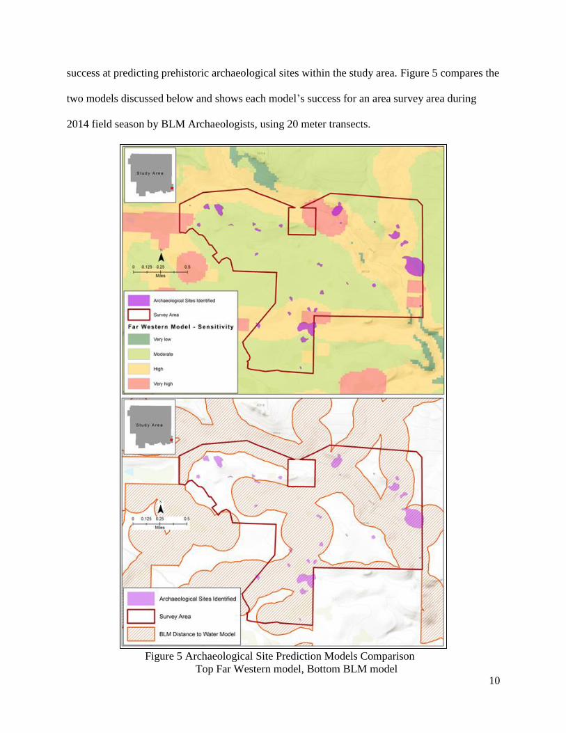
success at predicting prehistoric archaeological sites within the study area. Figure 5 compares the

two models discussed below and shows each model’s success for an area survey area during

2014 field season by BLM Archaeologists, using 20 meter transects.

Figure 5 Archaeological Site Prediction Models Comparison

Top Far Western model, Bottom BLM model

11

2.2.1. Far Western prehistoric site sensitivity model

Far Western Anthropological Research Group, Inc. was contracted by the BLM to

complete a report on the cultural resources of northeastern California and in 2004 they published

that report (King, et al. 2004). As part of that report they developed a Prehistoric Site Sensitivity

Model using the Weights of Evidence modeling technique. Weights of Evidence is a Bayesian

prediction method initially applied in medical diagnosis (Lusted 1968). This method was later

adapted to work with spatial data for use in geologic studies, treating raster cells as an ensemble

of independent models (Bonham-Carter 1994). Similar to logistic regression, Weights of

Evidence relies on the logistic transformation to deal with a continuous range of outcomes,

ranging from highly likely to highly unlikely (Bolstad 2010).

A Weights of Evidence model is trained on a set of specific points, the "training points",

in this case known archaeological sites, in combination with the corresponding evidential rasters

(King, et al. 2004). The map from Far Westerns report is displayed in Figure 6, the study area for

this project is the displayed as the BLM Field Office boundary in the north western corner. By

observing the presence and absence of training points in raster cells, weights are developed for

each cell of the evidential layer, the presence of training-points within a particular raster value

constitutes a positive weight, the absence of training-points a negative weight. Training points

will be associated with some values (positive weights) and not associated with other values

(negative weights) in an evidence layer. The “contrast” between the positive and negative

weights for an evidential layer is a strong measure of how predictive that layer is (King, et al.

2004). Although a proven modeling technique, Weights of Evidence was not chosen for this

project because the software is out of date and no longer compatible with the latest Esri software

which it needs to run.

12

Figure 6 Far Western Study Area and Ecological Zones (King, et al. 2004)

Far Western separated their study area into four ecological zones to better represent the

variability in ecological settings across the study area. The ecological zones were determined

based mainly watershed boundaries and vegetation communities, to account for environmental

differences across the study area (King, et al. 2004). They ran the Weights of Evidence model for

each of those ecological zones using slope, aspect, landform type, hydrologic features and

13

vegetation as the evidential layers. The archaeological site data was provided by the BLM, USFS

and the Northeast Information Center at California State University Chico. The resulting

sensitivity model was categorized as low (<0.5 times average site density), moderate (0.5 - 1.25

time average), high (1.25 - 3 times average) and very high (> 3 times average) (King, et al. 2004).

2.2.2. BLM Distance to water model

In 2007, the United States Forest Service (USFS) and the Bureau of Land Management

completed the Sage Steppe Ecosystem Restoration Strategy Draft Environmental Impact

Statement. This document was the first step in an effort by the USFS and BLM to restore

declining habitats on 6.5 million acres of Federal Land. In order to ensure that prehistoric

archaeology was preserved, while being able to complete restoration work on a large and diverse

area, the California SHPO requested the BLM create a predictive model to guide field work.

During a meeting of the BLM Northeastern California Archaeologists (NECA) group (Jenifer

Rovanpera, David Scott, Sharron-Marie Blood and Marilla Martin) in June 10, 2013, the

development of the model was discussed.

In 2010, the NECA group working with a BLM GIS specialist created a distance to water

model. The model initially had two parameters: (1) Distance from water source parameter, 200

meters from either side of a stream and surrounding a spring or natural water body; and (2) Slope

parameter, omitting any area with slope of 25 degrees or greater. During field surveys and testing

of the model it was decided that a large enough percentage of sites were falling outside the

model and the decision was made to remove the slope parameter from the model. The model

became purely a 200 meter buffer of water sources.

14

2.2.3. Review of existing models

The two models discussed in this section are very different and both have limitations in

predicting archaeology site locations. However, even with their great differences in approach,

they produce similar results at the project area scale, Table 1 shows the similarities with the

assumption that the BLM distance to water is comparable to the High and Very High sensitivity

categories of the Far Western model. This could be merely coincidence or an indicator that they

have a similar design flaw, not factoring in site type limits the ability of the model to produce

meaningful results.

Table 1 Existing Model Performance within Study Area

Model

Total Sites

within study

area

Sites within

high

probability

Percent

Found

BLM distance to water 1,467 1,050 72%

Far Western prehistoric

site sensitivity 1,467 1,045 71%

The BLM distance to water model makes assumptions about the importance of water to

prehistoric people. Assuming that all activities and necessities occur within a certain distance to

water sources is problematic. Water is necessary to sustain life, so being close to water is

important when selecting habitation sites. However, other activities that are also necessary to

sustain life, such as collecting or hunting for food, increase the likelihood of prehistoric people

moving away from water sources. Additionally, the availability of water on the landscape

changes seasonally and over longer periods of time due to variability in weather patterns and

climate.

Far Western’s model used vegetation as one of the evidential layers, vegetation has

changed drastically since the first prehistoric people inhabited the area 12,000 years ago. Large

15

changes in climate would have greatly affect the amount of rainfall, increased the size and

amount of lakes and meadows, which would have huge effects on vegetation communities. Far

Western also chose to omit tool stone sources as an evidence layer, even though the data was

available and the Weights of Evidence method used could report the success of the layer at

predicting sites (King, et al. 2004).

At a project scale the two models appear very similar and have varying success at

predicting archaeological site locations. For the project scale analysis shown in Figure 5,

prediction similarities are apparent between the two models: in the Far Western Weights of

Evidence model, water courses were a strong predictor and springs were not (King, et al. 2004).

Thus, the very high and high sensitivity areas are similar to the BLM water proximity model.

2.3 Maxent for Predicting Prehistoric Archaeology

The maximum entropy technique is what the Maxent software uses to make predictions.

Using a sample of locations within a defined area and a set of variables the Maxent technique

calculates a range of environmental values that are predictors of the sample locations, from that

range the distribution of maximum entropy is selected (Phillips, Dudík and Schapire 2004). A

presence only species data set, with spatial coordinates, multiple environmental variables and a

defined study area boundary are all that are need to run the Maxent software. What it predicts is

the environmental suitability across the study area by using the environmental conditions found

at each of the occurrence points (Phillips, Anderson and Schapire 2006). Maxent does multiple

iterations within a “black box” modeling technique, to optimize the suitability distribution (Kern-

Isberner, Wilhelm and Beierle 2014).

Maxent software was developed in 2004 by Phillips, Dudik and Schapire for use in

conservation of animal and plant species. Animal and plant species distribution is driven by

16

environmental variables. While human behavior is slightly less prone to environmental variables,

prehistoric people’s distribution is much more influenced by environmental variables than that of

modern people. This makes Maxent a good tool for predicting the environmental suitability of

locations for use by prehistoric people across the study area.

For this study the presence data is archaeological sites with locations recorded during

field survey. The environmental variables were selected based on King et al. 2009 and personal

communication with the BLM NECA group. Slope, aspect, distance to water sources, distance to

tool stone sources, distance to large game corridors and geologic units were selected to predict

the occurrence of prehistoric people across the study area.

Each of these environmental layers as well as the application of Maxent to these data are

next discussed in greater detail in Chapter 3.

17

Chapter 3 Methodology

In order to test the hypothesis, that using a site type model will be as good or a better predictor of

archaeological site location than an uncategorized model, the presence of site data was

categorized three different ways and three runs of the Maxent software were conducted. For each

run the environmental data remained the same. The following is a discussion of the geographic

context of the study area, the sources of each of the presence and environmental data layers, the

basis for the model set up and the tools that were used to assess and compare the models that

were produced.

3.1 Study Area

The study area, shown above in Figure 1, is the western portion of the Applegate Field

Office, BLM. It is located in northeastern California, containing 501,000 acres of public lands

managed by BLM and 1.9 million acres of USFS managed public lands. Ranging greatly in

ecological diversity, the study area contains pine forest, high desert plateau, wetlands,

grasslands, basalt lava flows and river basins. It ranges in elevation from approximately 3,000 to

7,500 ft. This is a rural area with no large cities. The largest disturbance to prehistoric sites since

the arrival of European settlers to the area has been from the clearing of land for agriculture as

Kniffen described in 1928.

3.2 Software

This project utilized Esri® ArcGIS™ version 10.3.1, including ArcMap and ArcCatalog

with the ArcGIS Spatial Analyst license. The XTools Pro version 11.1 toolbar for ArcGIS

desktop and Microsoft Excel® 2010 was also used in the preparation of data. The modeling was

18

done using Maxent version 3.3k. Maxent is a free software program available online for

download from Princeton University2.

3.3 Archaeology Site Location Data

Archaeology site location data has been collected within the study area in the form of site

records since the 1960s. Although this data is considered sensitive and is not provided to the

general public, it was graciously provided for use in this project by the BLM Applegate Field

Office, and the USFS (Modoc National Forest and Lassen National Forest) in the form of

ArcGIS geodatabases. Each of the three data sources is a combination of legacy data, data

digitized from 24k topographic maps and data collected with professional grade Global

Positioning Systems (GPS) devices. The data digitized from 24k topographic maps has an

accuracy of approximately 14 meters; the data collected with GPS devices has an accuracy of 10

meters or better. The majority of the data was collected during field survey of specific project

areas. These project specific surveys cause the data to have small clusters within the distributed

data as a whole. These clusters may influence the final Maxent output, this sampling bias may

cause the model to be weighted towards areas that have a higher number of samples (Phillips,

Dudík and Schapire 2004). Areas such as privately owned lands that have not been sampled, tend

to be areas around large water sources, lakes and rivers, as well as the most fertile lands for

agricultural production. Figure 7 shows the distribution of the archaeological site locations

across the study area.

2 https://www.cs.princeton.edu/~schapire/maxent/

19

3.3.1. Prehistoric Data Preparation for Maxent

Archaeological site presence data must be in a comma delineated text file with three

required fields, ‘species’, X-coordinate and Y-coordinate, to be compatible with the Maxent

software. The ‘species’ field allows for the categorization of site types: if all sites have the same

‘species’, this translates to the undifferentiated model, and if various ‘species’ (i.e. site types) are

given, this translates to multiple site types. The USFS data was in three formats, point, line and

polygon feature classes and the BLM data was in a polygon feature class. Both data sources

contained both historical as well as prehistoric data; for this study the historic data was removed.

The USFS data contained very little attribute information and could not be categorized into site

Figure 7 Archaeological Site Locations Map

20

types (e.g. ‘species’), while the BLM data had a large amount of attribute information which was

used to make site type categorizations. All data was projected into North American Datum 1983,

Universal Transverse Mercator (UTM) zone 10.

The polygon and line features were converted into point features using the Feature to

Point tool, in the Data Management toolbox within ArcMap. This tool converts the center point

of the feature into a point and exports the resulting data into a shapefile. To organize the site

location data for each of the three runs, the data was processed as follows. Table 2 summarizes

the resulting data prepared for Maxent.

1. The site type approach used only BLM site data because it was the only dataset that

contained attribute information about the artifacts and features at each site, providing

the basis to categorize by the type of site. There was sufficient attribute information

to create four categories, however due to the low number of sites in two of the

categories only the two with the highest number of sites were used. The categorized

point shapefile, was used as the ‘species’ input for the Maxent model.

2. The “kitchen sink” approach used all of the BLM and USFS site data and, using the

Merge tool from the Data Management toolbox, combined the individual layers into

one shapefile. The ‘species’ type distinction was not used for this run.

3. For the ecological approach, an Ecological Region layer was created (discussed in

further detail in Section 3.5). The ecological regions were intersected with the site

location point shapefile created for the kitchen sink approach, adding an ecological

region ‘species’ type to each site record.

The remaining steps were done for each of the three shapefiles created for the three

different approaches. The X and Y coordinates were calculated for each point within the attribute

21

table. The value at each point for each of the environmental evidence layers was also extracted

and added to the attribute table for each layer. The addition of this data helps Maxent run more

efficiently and save time. Each of the site datasets was then exported and converted into a

comma delineated text file.

Table 2 Archaeological Site Location Data

Maxent Run Data Source ‘Species’ Number of sites

Site Type BLM

Lithic Scatter 1,195

Rock Feature 137

Habitation* 90

Rock Art* 22

Eco Region BLM and USFS

Fall River 426

South Fork Pit River 1,029

Tule Lake 1,554

Warm Springs 720

Kitchen Sink BLM and USFS Archaeological Site 3,729 * These categories were not used because of the small amount of data

3.4 Environmental Evidence Layers

The environmental evidence layers used in this project were chosen because of the effect

they would have had on influencing the behavior of prehistoric people across the landscape. This

section discusses why each data category was chosen and the resulting layers. Table 3

summarizes the environmental variables and their data sources. Each of the environmental

variable layers must be in the form of an ASCII grid, with matching raster cell size and grid

placement to be compatible with the Maxent software. Esri ArcMap software allows for

geoprocessing environments to be set for all data processed within an ArcMap session and the

following environments were set: 1) Project all data into North American Datum 1983, UTM

Zone 10; 2) Clip all layers to the study area; 3) Raster analysis cell size of 30 meters; 4) Snap to

raster (aligned all raster grids to the aspect raster as this was the first raster created). This insured

22

that as all of the environmental evidence layers were identical, in shape, cell size, orientation,

and projection.

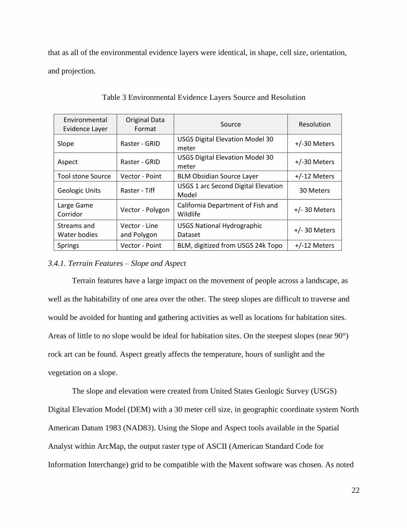
Table 3 Environmental Evidence Layers Source and Resolution

Environmental Evidence Layer

Original Data Format

Source Resolution

Slope Raster - GRID USGS Digital Elevation Model 30 meter

+/-30 Meters

Aspect Raster - GRID USGS Digital Elevation Model 30 meter

+/-30 Meters

Tool stone Source Vector - Point BLM Obsidian Source Layer +/-12 Meters

Geologic Units Raster - Tiff USGS 1 arc Second Digital Elevation Model

30 Meters

Large Game Corridor

Vector - Polygon California Department of Fish and Wildlife

+/- 30 Meters

Streams and Water bodies

Vector - Line and Polygon

USGS National Hydrographic Dataset

+/- 30 Meters

Springs Vector - Point BLM, digitized from USGS 24k Topo +/-12 Meters

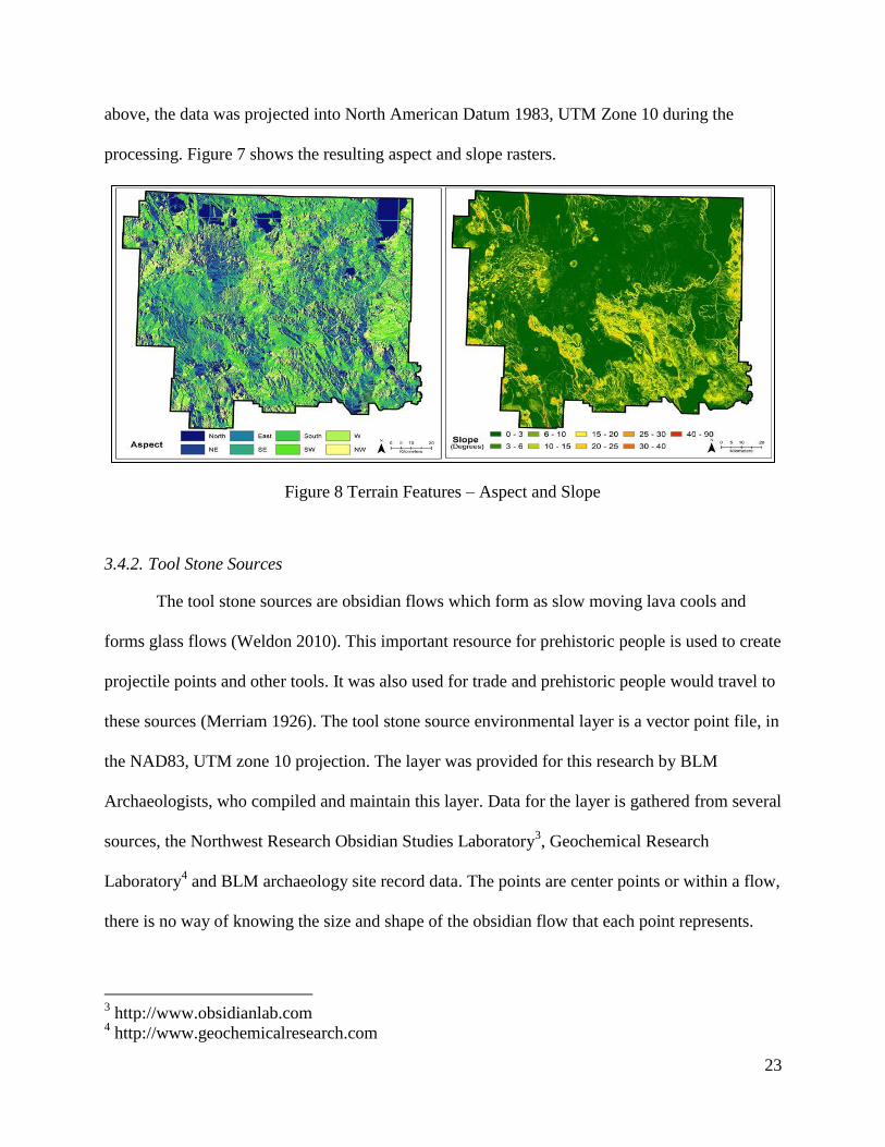
3.4.1. Terrain Features – Slope and Aspect

Terrain features have a large impact on the movement of people across a landscape, as

well as the habitability of one area over the other. The steep slopes are difficult to traverse and

would be avoided for hunting and gathering activities as well as locations for habitation sites.

Areas of little to no slope would be ideal for habitation sites. On the steepest slopes (near 90°)

rock art can be found. Aspect greatly affects the temperature, hours of sunlight and the

vegetation on a slope.

The slope and elevation were created from United States Geologic Survey (USGS)

Digital Elevation Model (DEM) with a 30 meter cell size, in geographic coordinate system North

American Datum 1983 (NAD83). Using the Slope and Aspect tools available in the Spatial

Analyst within ArcMap, the output raster type of ASCII (American Standard Code for

Information Interchange) grid to be compatible with the Maxent software was chosen. As noted

23

above, the data was projected into North American Datum 1983, UTM Zone 10 during the

processing. Figure 7 shows the resulting aspect and slope rasters.

3.4.2. Tool Stone Sources

The tool stone sources are obsidian flows which form as slow moving lava cools and

forms glass flows (Weldon 2010). This important resource for prehistoric people is used to create

projectile points and other tools. It was also used for trade and prehistoric people would travel to

these sources (Merriam 1926). The tool stone source environmental layer is a vector point file, in

the NAD83, UTM zone 10 projection. The layer was provided for this research by BLM

Archaeologists, who compiled and maintain this layer. Data for the layer is gathered from several

sources, the Northwest Research Obsidian Studies Laboratory3, Geochemical Research

Laboratory4 and BLM archaeology site record data. The points are center points or within a flow,

there is no way of knowing the size and shape of the obsidian flow that each point represents.

3 http://www.obsidianlab.com

4 http://www.geochemicalresearch.com

Figure 8 Terrain Features – Aspect and Slope

24

The tool stone sources layer had to be converted to a raster to use in Maxent. This was

done using the Euclidian Distance tool in Spatial Analyst within ArcMap. The Euclidian

Distance tool creates a continuous distance raster, where each cell’s value is the distance to the

nearest source. Using the environmental settings discussed earlier in this chapter, the raster was

created with a 30 meter cell size and clipped to the study area. It was then converted into the

ASCII grid format for use in Maxent. Figure 8 shows the resulting tool stone source raster.

3.4.3. Geologic Units

Geologic units were selected for this project because of the large amount of information

that can be inferred from the underlying geologic features. The geologic map unit gives

information on the age of geologic features. Basalt lava flows from the Pleistocene and Holocene

eras would mean active volcanic activity that would have been avoided by prehistoric people of

that period and they would have been free of vegetation for the period following. In later

prehistoric times geologic features are an indication of the possible soil depth and fertility.

Figure 9 Tool Stone Sources

25

The geologic unit layer is a vector polygon layer digitized from a 1:100,000 scale USGS

Geologic map of northeastern California, in geographic coordinate system NAD 1927. The layer

was converted from vector polygon to GRID raster using the Polygon to Raster tool in the

Conversion toolbox in ArcMap. The resulting raster has a 30 meter cell size, was clipped to the

study area and projected in NAD83, UTM zone 10. The raster was then converted into an ASCII

grid for use in Maxent, shown in Figure 9.

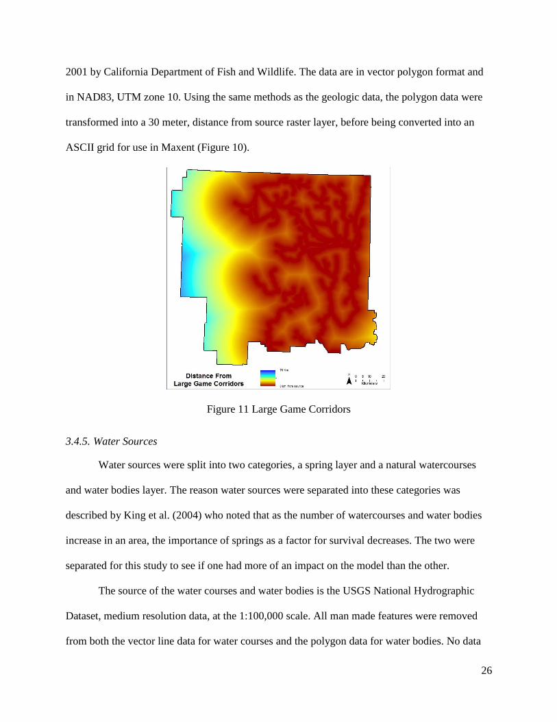
3.4.4. Large Game Corridors

The large game corridors are deer and pronghorn antelope migration corridors and

seasonal use areas. Large game provides an important food source that could feed many people

and for the Pit River tribe, large game drives involved multiple groups (Kniffen 1928).

Archaeological site records detail evidence of large game hunting within and near these

corridors, projectile points and a game drive (Scott and Oyarzun 2012). The data for large game

corridors used in this project were developed in the 1970s and then digitized and reviewed in

Figure 10 Geologic Units

26

2001 by California Department of Fish and Wildlife. The data are in vector polygon format and

in NAD83, UTM zone 10. Using the same methods as the geologic data, the polygon data were

transformed into a 30 meter, distance from source raster layer, before being converted into an

ASCII grid for use in Maxent (Figure 10).

3.4.5. Water Sources

Water sources were split into two categories, a spring layer and a natural watercourses

and water bodies layer. The reason water sources were separated into these categories was

described by King et al. (2004) who noted that as the number of watercourses and water bodies

increase in an area, the importance of springs as a factor for survival decreases. The two were

separated for this study to see if one had more of an impact on the model than the other.

The source of the water courses and water bodies is the USGS National Hydrographic

Dataset, medium resolution data, at the 1:100,000 scale. All man made features were removed

from both the vector line data for water courses and the polygon data for water bodies. No data

Figure 11 Large Game Corridors

27

was available about the width of the water courses so the water course lines were buffered by

one meter to convert the data into polygons and then merged with the polygon water body data.

The resulting layer was then converted into a 30 meter distance to water raster, using the same

methods as described earlier and then converted into the ASCII format for use in Maxent.

The spring data for this project was assembled from two sources, the BLM water source

improvements layer (collected with a professional grade GPS unit) and by digitizing from a

1:24,000 USGS topographic map. The two data sources were merged and the resulting distance

to springs layer was prepared in the same manner as the tool stone data layer described earlier in

this chapter. The resulting ASCII rasters for watercourses and water bodies, as well as for

springs is shown in Figure 11.

3.5 Other Data

The ecological regions were based off of the Far Western model ecological zones, shown

in Figure 6. However, for this project the ecological regions were adjusted to better represent a

Figure 12 Water Sources

Watercourses and Water Bodies on the left, Springs on the right

28

smaller study area than Far Western used. The USGS Watershed Boundary dataset, subbasins

were used for the basis of the layer. On the edges of the study area slivers of subbasins outside of

the study area boundary were combined to with subbasins within the study area. On the eastern

portion of the study area subbasins were divided based on the fifth level watershed boundaries, to

better represent the more cohesive environmental variables on the eastern side of the study area.

The resulting ecological regions are displayed in Figure 13.

Figure 13 Ecological Regions

3.6 Maxent Modeling

While the Maxent software is easy to use, with the input data in the correct format the

user must then set the parameters of the model to produce the best result for the data being

modeled. The following section outlines the model parameters selected and why those choices

29

were made. Within the software the user selects the ‘species’ to model (if any), the

Environmental layers, and output format and file type. In addition, the user can adjust settings for

each model run. The output for this project is Logistic, this output uses post processing to create

the probability that the ‘species’ will occur in each modeled location (Phillips, Dudík and

Schapire 2004).

For this project, in each of the three runs—site type, ecological regions and the “kitchen

sink”—the parameters were set the same, with the exception of the number of replicates run.

This decision was made based upon the time it would take for the model to run since replicates

are run for each ‘species’. Table 4 shows the number of replicates used for each of the three runs.

In order to produce the best results, over 20 test runs were made to evaluate different parameter

settings; only the parameters selected for the final runs are discussed here. Maxent also has many

available settings; only the selected settings or settings changed from the default settings are

discussed. Table 5 summarizes the selected parameters and the rationalization for each of those

selections.

Table 4 Replicates chosen for each Maxent run

Maxent Run Number of replicates Site Type (Species) Number of Sites

Site Type 25 Lithic Scatter 1,195

Rock Feature 137

Eco Region 10

Fall River 426

South Fork Pit River 1,029

Tule Lake 1,554

Warm Springs 720

Kitchen Sink 25 Archaeological Site 3,729

30

Table 5 Model Parameters

Parameter Selection/entry Rationalization

Create Response Curves

Selected Response curves display how each of the environmental variables performed for each ‘species’ run

Default Prevalence

0.8 Probability that a ‘species’ will occur at any occurrence point. Based on archaeology survey data, the probability is high that there will be an occurrence within an occurrence raster cell. Default is 0.5

Jackknife Selected Test determines the importance of each environmental variable

Maximum Iterations

500 Iterations of optimization algorithm, the more iterations the more the model is trained

Random Seed Selected Different set of random points are selected for test and training samples

Random Test Percentage

20 Percent of random points set aside for testing the model

Regularization Multiplier

5 More evenly distributed probability as this number increases (default is 1)

Replicated Run Type

Bootstrap Uses 20% of randomly selected points for each of the replicates

Replicates See Table 4 Numbers chosen to be high enough to create average and median outputs, while remaining small enough for the Maxent to run in a reasonable amount of time

Although the number of replicates as well as the number of sites varies for each of the

runs, the built-in model validation tools provide enough information that the runs can be

compared. The Receiver Operating Characteristic (ROC) curve, Area Under the ROC Curve

(AUC), response curves and jack-knife testing, assess the models overall performance as well as

that of each of the environmental evidence layers (Phillips n.d.). All of these results are discussed

in the next chapter.

31

Chapter 4 Results

Three runs were conducted using the Maxent software program, each using the same Maxent

parameter settings as well as the same environmental evidence rasters and varying “species” or

site type presence point locations. This chapter discusses the output of each of the three runs and

assesses the fit of each model using the results of the built-in validation tools. The final product

is a probability distribution map that Maxent produces for each ‘species’ model run.

4.1 “Kitchen Sink” Results

The “kitchen sink” approach ran 25 replicates and only one ‘species’ type, archaeological

site, of which there were 3,729 sites. Using the bootstrap method, 20% of the total sites were

held back during each replicate run for testing.

Maxent provides some very important information in the output of the model run for

assessing for each environmental factor and the model as a whole. The percent contribution of

each environmental variable, how much that variable contributed each of the presence point

locations is summarized in Table 6. It also gives the permutation importance, which tests how

the model reacts if the values of that variable were altered (Phillips n.d.). Given this information,

the stability of each environmental factor can be assessed, an unstable variable has high percent

contribution and a high permutation value. A stable variable has high percent contribution and a

low permutation importance. Geologic unit had the largest percent contribution and a moderately

high permutation importance. Distance from game corridor had a moderately high percent

contribution and very high permutation importance value. Over all the environmental variables

are fairly unstable.

32

Table 6 “Kitchen Sink” environmental variables

Variable Archaeological Site

Percent

contribution Permutation importance

Geologic Unit 39% 12.8

Distance from watercourses and water bodies 23% 15.1

Distance from large game corridors 16% 31.0

Distance from tool stone sources 9% 15.6

Slope 8% 14.6

Distance from springs 3% 8.5

Aspect 2% 2.2

Another important test of the overall model performance is the ROC and AUC. The AUC

tells how well the model is able to predict the difference between the presences and random. The

model fit can be determined based on how close the AUC is to 1. Maxent averages the AUC

from each of the 25 replicates runs to come up with the AUC for the model. This model has an

AUC of 0.793 with a standard deviation of 0.003, shown in Figure 12. This model performed

well.

Figure 14 “Kitchen Sink” AUC

33

4.2 Ecological Region Results

The ecological region approach ran 10 replicates of the four ecological regions, Fall

River (426 sites), South Fork Pit River (1,029 sites), Tule Lake (1,554 sites) and Warm Springs

(720 sites). Using the bootstrap method 20% of the total sites for each ecological region where

held back during each replicate run for testing. The following is the results of the Maxent

assessment of the ecological region variables and the fit of the model AUC.

The percent contribution of each environmental variable, how much that variable

contributed each of the presence point locations is summarized in Table 7. Distance to tool stone

contributes the most to the model for each of the four ecological region models. For the Fall

River and South Fork Pit River Models distance to tool stone is very unstable, but in the Tule

Lake and Warm Springs models it is very stable.

Table 7 Ecological region environmental variables

Variable Fall River South Fork

Pit River Tule Lake

Warm Springs

Pe

rce

nt

con

trib

uti

on

Pe

rmu

tati

on

imp

ort

ance

Pe

rce

nt

con

trib

uti

on

Pe

rmu

tati

on

imp

ort

ance

Pe

rce

nt

con

trib

uti

on

Pe

rmu

tati

on

im

po

rtan

ce

Pe

rce

nt

con

trib

uti

on

Pe

rmu

tati

on

imp

ort

ance

Geologic Unit 5% 0.7 0.4% 0.7 2% 18.1 3% 2.3

Distance from watercourses and water bodies

15% 22.8 12% 10.0 12% 10.3 11% 5.1

Distance from large game corridors

5% 2.1 8% 13.7 12% 28.8 16% 49.5

Distance from tool stone sources

72% 64.1 71% 63.3 63% 10.5 54% 1.1

Slope 0.9% 1.0 2% 6.4 6% 25.3 9% 14.3

Distance from springs 0.5% 9.3 0.4% 5.8 6% 4.7 7% 26.8

Aspect 0.1% 0.1 0.1% 0 0.3% 2.4 0.4% 0.9

34

The AUC for each of the four ecological region models show that each model performed

very well, with the South Fork model having the best fit. The AUC and standard deviations are

displayed in Table 8.

Table 8 Ecological region AUC

Fall River

South Fork Pit River

Tule Lake Warm Springs

Mean AUC

0.882 0.903 0.852 0.823

Standard Deviation

0.007 0.004 0.007 0.007

4.3 Archaeological Site Type Results

The site type approach ran 25 replicates of the two site types, lithic scatter (1,195 sites)

and rock features (137 sites). Using the bootstrap method, 20% of the total sites for each of the

site types where held back during each replicate run for testing. The following is the results of

the Maxent assessment of the environmental variables and the fit of the model AUC.

The percent contribution of each environmental variable, how much that variable

contributed each of the presence point locations is summarized in Table 9 for the archaeological

site types. Distance to large game corridors contributes the most to the model for each of the site

type models. Distance from tool stone sources is also a high contribution to the models of both

site type model and is a much more stable indicator.

35

Table 9 Site type environmental variable

Variable Lithic

Scatter Rock

Features

Pe

rcen

t co

ntr

ibu

tio

n

Pe

rmu

tati

on

im

po

rtan

ce

Pe

rcen

t co

ntr

ibu

tio

n

Pe

rmu

tati

on

imp

ort

ance

Geologic Unit 5% 1.4 5% 3.7

Distance from watercourses and water bodies

16% 26.5 12% 13.0

Distance from large game corridors

48% 17.4 47% 41.8

Distance from tool stone sources 21% 32.2 15% 5.3

Slope 5% 2.1 7% 20.9

Distance from springs 5% 19.9 11% 14.1

Aspect 1% 0.5 3% 1.1

The AUC for each of the site type models show that each model performed very well,

with the rock features having the best fit of the two models. The AUC and standard deviations

are displayed in Table 10.

Table 10 Archaeological Site Type AUC

Lithic

Scatter Rock

Features

Mean AUC 0.86 0.905

Standard Deviation

0.003 0.011

36

4.4 Probability Distribution

Maxent produces an ASCII raster of the probability distribution. It is an average of the

replicates for each of the ‘species’ run. Each map displays a continuous probability distribution

raster where the probability of a site occurring is calculated for each 30 meter cell. Figures 13, 14

and 15 display the resulting rasters for the “Kitchen Sink”, ecological region and archaeological

site type respectively.

Figure 15 “Kitchen Sink” Probability Distribution Map

The probability distribution for the “kitchen sink” model, displays how the high percent

contribution from geologic unit, distance from watercourses and water bodies and distance from

37

large game corridors contributed to the distribution, with the highest probabilities falling within

one geologic type and within areas close to water and game corridors. Also, visible in the map is

the areas with the lowest and highest percent slope are lower probability.

Figure 16 Ecological Region Probability Distribution Maps

Each of the four ecological region probability distributions maps display the high percent

contribution of distance from tool stone sources. Tule Lake, Warm Springs and South Fork Pit

River highest probability areas correlate to areas close to tool stone sources. For the Fall River

model the highest probability area correlates to the area farthest away from tool stone sources.

38

Figure 17 Site Type Probability Distribution Maps

39

The site type probability distribution maps, lithic scatter and rock features, both show a

strong correlation with large game corridors, which had the highest percent contribution to both

models. The lithic scatter probability map also shows a strong connection to tool stone sources,

the highest probability areas are close to sources. The rock feature probability distribution also

shows high probability areas that are moderate slopes, while very steep and flat areas are low

probability.

4.5 Evaluation of Maxent Models

Each of the three Maxent runs had their own set of successes and challenges. In this

section the models are evaluated for the whole study using the tools built into the Maxent

software. The models are also evaluated for the project scale, using an area surveyed at 20 meter

transects and all sites within the survey area recorded. Each evaluation provides important

information on the reliability of Maxent for predicting archaeological site locations. The study

area scale evaluation gives an idea of how statistically sound each model is and the influence of

each environmental variable for predicting archaeological site locations. The project scale

evaluation gives an idea of how successful each model is at the project scale and gives the

opportunity to compare the Maxent model against the Far Western and BLM archaeological site

prediction models.

4.5.1. Study Area Evaluation

At the study area scale, all three models performed very well, when only taking into

account the AUC. The closer the AUC is to 1 the better the fit of the model is. As hypothesized,

the “kitchen sink” model run had the lowest AUC of 0.793 with a standard deviation of 0.003.

The ecological site and site type models preformed similarly with the AUC ranging from 0.823

to 0.905 on all the models. The percent contribution and permutation importance give a better

40

idea of how successful these models are from an archaeological context. Table 11 summarizes

the environmental variables with the highest percent contribution for each of the model runs. It is

important to keep in mind that the lower the permutation importance values the more stable the

environmental variable.

Table 11 Model Percent Contribution Comparison

Percent

contribution Permutation importance

"Kit

chen

Si

nk"

Variable Archaeological Site

Geologic Unit 39% 12.8

Distance from watercourses and water bodies 23% 15.1

Eco

logi

cal R

egio

n

Fall River

Distance from tool stone sources 72% 64.1

South Fork Pit River

Distance from tool stone sources 71% 63.3

Tule Lake

Distance from tool stone sources 63% 10.5

Warm Springs

Distance from tool stone sources 54% 1.1

Site

Typ

e

Lithic Scatter

Distance from large game corridors 48% 17.4

Distance from tool stone sources 21% 32.2

Rock Features

Distance from large game corridors 47% 41.8

Distance from tool stone sources 15% 5.3

Geologic unit and distance from watercourses and water bodies had the highest

contribution to the “kitchen sink” model. This makes sense when considering what would be

important factors for any type of site use. At a landscape level, prehistoric people would be more

inclined to select sites that are close to water sources and have less volcanic rock, making them

more easy to traverse and more likely to have fertile soils for food sources as well as being

habitat for game. The percent contribution was much more distributed over all of the

41

environmental variables for the “kitchen sink” model, this is most likely because this model only

took into account that an archaeological site existed at each location but not what the use was at

that site.

While the ecological region models were very successful from the perspective of the

statistical tools within Maxent, this is very misleading. Sites were categorized based on an

ecological region, so the sites used for each model were grouped in one portion of the study area.

The models should only be considered valid for the ecological region that they represent, as

shown in Figure 16. The highest percent contribution for each of the models was distance from

tool stone. However, the Fall River and the South Fork Pit River model have a very high

permutation importance, so tool stone is a very unstable predictor of archaeological site

probability. Figure 18 shows the distribution of tool stone sources and the distribution of

archaeological sites within each ecological site.

Figure 18 Ecological Regions and Distance from Tool Stone

42

The site type models are the most successful of the three runs. The highest percent

contribution for the lithic scatter model is distance from large game corridor which is a fairly

stable predictor. The second highest percent contribution is distance from tool stone sources,

however this is much less stable predictor than the distance from large game corridors. The rock

features model had the same two environmental variables with the highest percent contribution,

with distance to tool stone sources being the more stable of the two.

The highest percent contribution from distance from large game corridors and distance

from tool stone sources shows the success of the site type method. Lithic scatters are the remains

of creating tools and projectile points from tool stone sources, so these two variables being the

highest percent contribution are archeologically sound. Rock features are any rock placement,

rock stack, rock alignment, hunting blinds or other rock feature. These features could be

associated with hunting, either directly hunting blinds and rock alignments that were used for

large game drives, or indirectly, rock stacks used for navigation.

4.5.2. Project Scale Evaluation

The project scale survey example can be used to evaluate how the Maxent models

compare to the previous models, Far Western and the BLM distance to water model. Each of the

previous models captured over 70% of the sites within the high probability area of the models for

the whole study area. The project scale performance of the Far Western and BLM models were

discussed in Chapter 2 where Figure 5 shows the previous models’ performance at the project

scale within the survey area. This section looks at the performance of each of the Maxent models

for the same survey area, because the survey area was within the South Fork Pit River ecological

region, that was the only ecological region model that was used for comparison.

43

The survey area is approximately 5,800 km2 (square kilometers) and after a being

surveyed using 20 meter transects, approximately 203 km2 of sites were recorded. Table 12

compares the area, in km2, of recorded sites and how they fell within each of the models. It is not

possible to compare the Maxent models directly to the Far Western and BLM models because

the categories are different. However, in Chapter 2 the assumption was made that the BLM

modeled area was comparable to the High and Very High categories from the Far Western

model. For this section the assumption is made, for comparison purposes, that <50% probability

is Very Low, 50-70% is Moderate, 70-90% is High and 90-100% is Very High. Using this

assumption, the South Fork Pit River, lithic scatter and “kitchen sink” were better predictors at

the project scale than the BLM, Far Western and rock features models. Each of these models is

discussed in further detail below.

Table 12 Survey Area Model Performance

Model Square kilometers of area containing sites

Very Low Moderate High Very High

Percent Probability < 50% 50-60% 60-70% 70-80% 80-90% 90-100%

"Kitchen Sink" 0 0 2 134 46 21

Lithic Scatter 1 0 3 1 130 68

Rock Features 165 32 2 4

South Fork Pit River 0 0 1 1 194 7

Sensitivity Very Low Moderate High Very High

Far Western 0 90 94 19

Modeled Area Outside Within

BLM 33 170

44

The survey area probability distribution maps for each of the models are discussed

below. Each map shows the recorded sites outlined and overlaid on the probability distribution.

The warmer colors indicate higher probability of an archaeology site and the cooler colors lower

probability. The “kitchen sink’ performed well with 201 km2 of the 203 km

2 of areas containing

recorded sites falling in the High and Very High probability areas and only 2 km2

falling within

the moderate range. The majority of the survey area is categorized as above 70% probability

area; this is displayed in Figure 19. As the probability distribution map shows, even the 2 km2

is

only a small portion of two sites and portions of the same sites also fall within the high

probability area.

Figure 19 Evaluation of “kitchen sink” model within survey area

For the ecological models, the only model evaluated is the South Fork Pit River. All but

two of the sites are within 80% probability and above, this is 201 km2 out of the total 203 km

2

45

surveyed. The remaining 2 km2 fall within the 60 to 80% range. For the South Fork Pit River

model the majority of the survey area is categorized as 80% probability and above, this is

displayed in Figure 18. The probability distribution map shows that the 2 km2 is one small site on

the eastern edge of the study area, all other recorded sites are completely within high probability.

The site type models, lithic scatters and rock features must be evaluated by taking into

consideration the type of site that was located during the survey. In Figures 21 and 22 the site

types are symbolized differently to show which sites were labeled as lithic scatters and what

were labeled as rock feature. The lithic scatter model performed very well with 199 km2 of the

surveyed sites within High and Very High probability. The rock features model performance was

the least successful of all the models with 156 km2 within the Very Low and 43 km

2 within

Moderate probability. Rock features had the least amount of archaeological site locations put in

to train the model, only 137 rock features were labeled within the entire project study area. Only

Figure 20 Evaluation of ecological region model within survey area

46

4 sites labeled as rock features fell within the survey area and are indicated on the probability

distribution map by the blue outline, the pink outlines are the lithic scatter type labeled sites.

Figure 21 Evaluation of site type, lithic scatter model within survey area

47

4.5.3. Discussion

The study area and project scale evaluations produced different results. At the study area

scale, the Maxent rock feature site type model performed the best, at the project scale the same

model performed the worst. The “kitchen sink’ was the least successful at the study area scale

and was very successful at the project scale. The lithic scatter and South Fork Pit River models

performed well at both scales. With the exception of the rock features model, all the other

Maxent models outperformed the Far Western and BLM models at the project scale. These

results indicate that Maxent can be used as a tool for predictive modeling of prehistoric

archaeology, however some improvements should be made. The variability of success for the

rock feature model may be attributed to this model having the lowest number of archaeological

site locations to train the model, 137 sites compared to over 1,000 for the lithic scatter and South

Fork Pit River and over 3,700 for the “kitchen sink” model. It is possible that this behavior

Figure 22 Evaluation of site type, rock features model within survey area

48

suggests that too few sites do not provide sufficient data to train the model, while too many

uncategorized sites may confuse the model. This possible explanation is depicted in Figure 23.

Figure 23 Model Success Curve

49

Chapter 5 Conclusions

The purpose of this project is to achieve reliable archaeological site predictions with the Maxent

software. To do this the following hypothesis was tested, that the site type Maxent model is as

good or a better predictor of archaeological site probability than Maxent models that do not

categorize by site type. The site type Maxent model will also be as good or a better predictor of

archaeological sites than the previous models at a project scale. This Chapter discusses the

results of the Maxent models produced and how archaeological site prediction models may be

improved in the future for the study area.

5.1 Discussion

An archaeological site prediction model is one important tool that can be used to help

preserve and tell the story of the prehistoric people that lived on this land. Predicting human

behavior is a daunting task and predicting the behavior of 11,000 years of prehistoric people

within this study area will never be completely accurate. As discussed in Chapter 4, this project

has shown that the Maxent method of modeling provides a successful method for predictive

modeling of archaeology site locations for the study area, with some additional work being

needed. The Maxent models, for the most part, improved on the Far Western and BLM models

and were shown to be reliable using the tests built into the Maxent software and within the

project level survey example.

The evaluation of the models were not enough to prove or disprove the hypothesis,

further work is needed to make a definitive argument. Although, site type approach did perform

well with high AUC numbers for each of the four site type models, there are not enough

categorized sites to say definitively that the site type model will perform better at the project

50

scale than the two previous models. This project was able to prove the value of the commitment

by the BLM to input archaeological site attribute information into a spatial database.

5.2 Limitations

This project was limited by the completeness of the attribute information for the

archaeology site location data, because the data was provided by two different government

agencies data formats and the level of attribute information varied. However, because the BLM

and the USFS are both federal government agencies, the data collected in the field for each site

and entered into site records is similar and could be entered into a spatial database producing a

consistent data layer for the entire study area. This would make it possible to run the site type

modeling approach using all the known archaeology site locations.

Another data limitation of this project is the lack of archaeology site location data on

privately owned lands. As discussed in Chapter 3, no data is available for archaeology site

locations on private lands and because areas of fertile agricultural lands and surrounding large

water bodies and rivers are more likely to be privately owned, this lack of data may cause a

sampling bias. If archaeology surveys were conducted randomly across the landscape, including

all ownership and environment settings, this would limit the survey bias and could improve

modeling success.

5.3 Future Work

Further work with archaeologists is needed in order to get the required classifications of

prehistoric archaeology sites and to further improve the modeling results. Enough data exists

within the study area, with over 3,000 sites, however only around 1,400 sites had sufficient

attribute information to be categorized with the site type. The site type information does exist

within site records for each of these sites, it would be a time intensive, but important task to input

51

this data into a useable format for modeling. With more attribute information more site type

categories could be used for modeling. If that work were to be completed, the hypothesis could

be tested and a definitive conclusion could be made.

There may be other environmental variables that could improve or be better predictors of

archaeology sites within the study areas. As more research and field survey is conducted by

archaeologists, better information on environmental factors may be available. Also, the quality of

environmental variable information could improve in the future. As these advancements are

made predictive archaeological site models should be continuously updated and approved upon.

5.4 Conclusion

The California SHPO requested a predictive model be developed by the BLM to assist

northern California archaeologists in their inventory efforts, specifically to direct field surveys.

The study area has a large amount of known prehistoric archaeology sites, many of these known

sites are eligible for listing on the National Register of Historic Places because of their value to

provide important information on how the people of the past lived. Only a small fraction of the

study area has been surveyed, so thousands of additional sites remain undiscovered. These sites

could contain important and never before discovered information on the life of prehistoric people

and are degrading over time because of natural elements, erosion and human activities. The cost

of surveying and finding important archaeology sites on millions of acres of land is huge. This

project demonstrated that using known site locations and environmental variables can successful

predict where to inventory for important sites. Implementing this modeling approach and doing

the future work described in the previous section could save federal land management agencies

and taxpayers millions of dollars. This approach will also lead to more important sites being

located and the sites and artifacts studied to increase understanding of prehistoric people.

52

References

Bolstad, William M., 1943. Understanding computational bayesian statistics. 1st ed. Hoboken,

N.J: Wiley.

Bonham-Carter, Graeme. 1994. Geographic information systems for geoscientists: Modelling

with GIS. 1st ed. Vol. 13. Oxford ;New York: Pergamon.

Carpenter, Kimberly L. 2002. "Reversing the Trend: Late Holocene Subsistence Change in

Northeastern California." in Boundary Lands: Archaeological Investigations Along the

California-Great Basin Interface, edited by Kelly R. McGuire. 49-59. (Nevada State

Museum Anthropological Papers, 2002).

Elith, Jane, Steven J. Phillips, Trevor Hastie, Miroslav Dudik, Yung En Chee, and Colin J. Yates.

2011. A statistical explanation of MaxEnt for ecologists. Diversity and Distributions 17

(1): 43.

M. Thomas P. Gilbert, Dennis L. Jenkins, Anders Götherstrom, Nuria Naveran, Juan J. Sanchez,

Michael Hofreiter, Philip Francis Thomsen, et al. 2008. DNA from pre-clovis human

coprolites in oregon, north america. Science 320 (5877): 786-9. Green, Dee F., and

Robert J. Laacke. Predictive Models for Locating Prehistoric Travel Pathways and

Campsites. Warner Mountain Rager District: USDA Forest Service, 1998.

Kailihiwa, Solomon Ha'aheo, III. 2015. “Using Maxent to Model the Distribution of Prehistoric

Agricultural Features in a Portion of the Hōkūli‘a Subdivision in Kona, Hawai‘i.”

Master's thesis, University of Southern California.

Kemp, Karen K. 2012. The Hawai'i Island Crop Probability Map: An Update of the Crop

Growth Parameters for the Hawai'i County Crop Model: Final Report Prepared for the

County of Hawai'i Researcy and Development Department. GIS Research Laboratory.

Kern-Isberner,Gabriele, Marco Wilhelm, and Christoph Beierle. 2014. “A Novel Methodology

for Processing Probabilistic Knowledge Bases Under Maximum Entropy.” Florida

Artificial Intelligence Research Society Conference. Key Larg, Florida, May 16-18.

King, Jerome, Kelly McGuire, Kimberley Carpenter, Mary Maniery, Cindy Baker, Hellen

McCarthy, Heather Scotten. 2004. Class I Cultural Resources Overview and Research

Design for the Alturas, Eagle Lake, and Surprise Resource Areas. Class I Cultural

Resources Overview, Davis, California: Far Western Anthropological Research Group,

Inc.

Kniffen, Fred B. "Achomawi Geography." University of California Publication in American

Archaeology and Ethnology 23, no.5 (1928): 279-332.

52

53

Merow, Cory, Matthew J. Smith, and John A. Silander. 2013. A practical guide to MaxEnt for

modeling species’ distributions: What it does, and why inputs and settings matter.

Ecography 36 (10): 1058-69.

Merriam, Dr. C. Heart. 1926."Classification and Distribution of the Pit River Indian Tribes of

California." Smithsonian miscellaneous collections. Vol. 78, No. 3.

Phillips, Steven J. n.d."A Brief Tutorial on Maxent." Unpublished documentation of the Maxent

software.

Phillips, Steven J., Miroslov Dudík, and Robert E. Schapire. 2004. "A maximum entropy

approach to species distribution modeling." Proceedings of the Twenty-First

International Conference on Machine Learning. 655-662.

Phillips, Steven J., Robert P. Anderson, and Robert E. Schapire. 2006. Maximum entropy

modeling of species geographic distributions. Ecological Modelling 190 (3): 231-59.

Scott, David J., and Megan C. Oyarzun. 2012."A big game procurement site, western toe of the

Warner Mountains, Rock Spring, Modoc County, California." 33rd Biennial Great Basin

Anthropological Conference, Poster Presentation. Stateline, Nevada, October 18-21.

Survey, US Geologiv. 2005. Preliminary Integrated Geologic Map Databases for the United

States: Western States: California, Nevada, Arizona, Washington, Oregon, Idaho, and

Utah. U.S. GEOLOGICAL SURVEY OPEN-FILE REPORT 2005-1305.

USDA Forest Service, USDI Bureau of Land Management. 2007.Sage Steppe Ecosystem

Restoration Strategy Draft Environmental Impact Statement. Environmental Impact

Statement, Alturas, CA: Modoc National Forest.

Weldon, K. 2010. Obsidian: Hotter Side of Obsidian.

http://volcano.oregonstate.edu/book/export/html/205 (accessed April 2, 2016).