predicted robustness as qos for deep neural network models
TRANSCRIPT

Wang YH, Li ZN, Xu JW et al. Predicted robustness as QoS for deep neural network models. JOURNAL OF COMPUTER
SCIENCE AND TECHNOLOGY 35(5): 999–1015 Sept. 2020. DOI 10.1007/s11390-020-0482-6
Predicted Robustness as QoS for Deep Neural Network Models
1State Key Laboratory for Novel Software Technology, Nanjing University, Nanjing 210023, China2Department of Computer Science, University of Surrey, Guilford, GU2 7XH, U.K.
E-mail: {wangyuehuan, lizenan}@smail.nju.edu.cn; {jingweix, yuping}@nju.edu.cn; [email protected]: [email protected]
Received March 31, 2020; revised July 29, 2020.
Abstract The adoption of deep neural network (DNN) model as the integral part of real-world software systems neces-
sitates explicit consideration of their quality-of-service (QoS). It is well-known that DNN models are prone to adversarial
attacks, and thus it is vitally important to be aware of how robust a model’s prediction is for a given input instance. A
fragile prediction, even with high confidence, is not trustworthy in light of the possibility of adversarial attacks. We propose
that DNN models should produce a robustness value as an additional QoS indicator, along with the confidence value, for
each prediction they make. Existing approaches for robustness computation are based on adversarial searching, which are
usually too expensive to be excised in real time. In this paper, we propose to predict, rather than to compute, the robust-
ness measure for each input instance. Specifically, our approach inspects the output of the neurons of the target model
and trains another DNN model to predict the robustness. We focus on convolutional neural network (CNN) models in the
current research. Experiments show that our approach is accurate, with only 10%–34% additional errors compared with the
offline heavy-weight robustness analysis. It also significantly outperforms some alternative methods. We further validate the
effectiveness of the approach when it is applied to detect adversarial attacks and out-of-distribution input. Our approach
demonstrates a better performance than, or at least is comparable to, the state-of-the-art techniques.
Keywords deep neural network, quality of service, robustness, prediction
1 Introduction
Deep learning (DL) has been demonstrated surpris-
ing power in various challenging tasks such as natu-
ral language processing [1], speech recognition [2], image
processing [3], recommendation systems [4, 5], gaming [6]
and even in the sentiment analysis for human beings [7],
which are hard to accomplish using conventional meth-
ods. Consequently, deep neural network (DNN) mod-
els are increasingly adopted in real-world applica-
tions, including some safety-critical scenarios such
as self-driving [8], disease diagnosis [9], and malware
detection [10].
However, different from conventional software arti-
facts, DNN models provide little guarantee about their
quality of service (QoS) on each individual input other
than the inaccurate confidence value [11, 12]. This is
largely due to the inductive nature of statistical ma-
chine learning and the lack of interpretability for DNN
models [13, 14]. Note that statistical metrics such as ac-
curacy, mean squared error (MSE), and F1-measure
actually report the model’s performance on the testing
data, but not how well it works on a new, unseen input.
A particularly naughty problem is that DNNs can
be easily fooled by adversarial examples, which are
Regular Paper
Special Section on Software Systems 2020
A preliminary version of the paper was published in the Proceedings of Internetware 2019.
This work was supported by the National Basic Research 973 Program of China under Grant No. 2015CB352202, the Na-tional Natural Science Foundation of China under Grant Nos. 61690204, 61802170, and 61872340, the Guangdong Science andTechnology Department under Grant No. 2018B010107004, the Natural Science Foundation of Guangdong Province of China un-der Grant No. 2019A1515011689, and the Overseas Grant of the State Key Laboratory of Novel Software Technology under GrantNo. KFKT2018A16.
∗Corresponding Author
©Institute of Computing Technology, Chinese Academy of Sciences 2020
Yue-Huan Wang1, Ze-Nan Li1, Jing-Wei Xu1,∗, Member, CCF, ACM, Ping Yu1, Member, CCF, Taolue Chen1,2
and Xiao-Xing Ma1, Member, CCF, ACM, IEEE

1000 J. Comput. Sci. & Technol., Sept. 2020, Vol.35, No.5
constructed by introducing well-designed human im-
perceptible perturbations to legitimate examples [15, 16].
The vulnerability to adversarial attacks is prevalent for
DNN models, and currently there is no general method
to eliminate them despite a plethora of proposals [17, 18].
The robustness of a DNN model, which quantifies the
model’s resilience to adversarial attacks, has attracted
a lot of attentions from both machine learning and soft-
ware engineering communities [19, 20]. Nevertheless, the
existing work merely aims at improving the training of
models and carries out offline robustness analysis, ren-
dering it unsuitable as an instant QoS indication for
the model’s prediction on the current input. The study
of adversarial attacks and robustness of DNN models is
somewhat predominately targeted at CNN models. In
this paper, for a better comparison with other methods,
we focus on CNN models for image classification tasks
as well.
In contrast, in this paper, we propose online cal-
culation of the robustness for each input at runtime.
Whenever a DNN model makes a prediction for an in-
put, a robustness value is quickly estimated to indicate
how stable the prediction is, against perturbations over
this input. This quality metric is important for the
system and users to decide how much the prediction
can be trusted, considering the possible perturbation
introduced intentionally or unintentionally. Note that
the robustness metric is not subsumed by prediction
confidence because of the existence of high-confidence
adversarial examples [15]. Robustness estimation is also
different from outlier detection [20, 21]. The former fo-
cuses on the stableness of the current model’s computa-
tion on the current input, while the latter measures the
rareness of an input compared with the whole dataset.
Nevertheless, as to be shown in Section 4, we can ex-
ploit robustness to detect outliers effectively.
The challenge of online robustness estimation is that
it needs to be very lightweight to exercise at runtime.
While DNN models are usually trained with power-
ful computers, they are often deployed in environments
with very limited computing power such as mobile and
embedded devices. For example, TensorFlow Lite 1○
and PyTorch Mobile 2○ support the DNN model exe-
cution on mobile devices, but not model training. And
while the training process can take hours, and even days
or weeks, a trained model gives instant prediction on in-
puts. The efficiency of robustness calculation needs to
match the instant model prediction.
Existing approaches to the robustness analysis are
based on either formal verification or adversarial search-
ing. Both of them are too heavy-weight for our purpose.
Formal verification approaches take the DNN model as
a usual (loop-free) program and try to prove that the
output of the model will not change if the perturbation
to input is within a small bound. These approaches
are computationally expensive owing to the nonlinear
structure of DNNs and the high dimensionality of input
data. Katz et al. [19] showed that the problem of verify-
ing robustness for ReLU networks is NP-complete. De-
spite interesting proposals of leveraging advanced SMT
solvers [19, 22] and abstract interpretation [23], currently
DNN robustness verification can handle only simple
DNN models with very limited perturbation bounds,
which makes them impractical for real-world applica-
tions.
Adversarial searching approaches apply optimiza-
tion to synthesize adversarial attacks with perturbation
as small as possible. The minimum perturbation realiz-
ing attack found within a time budget provides a met-
ric for the robustness of the DNN model [24]. Although
these approaches scale up to large DNN models, their
computation costs are still prohibitively high when used
at runtime (more than 10 hours for C&W applied on
ResNet-50).
We propose to learn a robustness predictor for each
trained DNN model offline. At runtime, for each input
fed to the model, one may use the robustness predictor
to predict how robustness the model is on this input
online. The insight behind this approach is two-fold.
First, robustness is a property about the target DNN
model’s behavior, which can be observed from the out-
puts of neurons in the model. Second, the theory of
representation learning [13] suggests that deep layers of
the target model encode its perception of the input, and
thus are informative for the model’s robustness on the
input. Therefore we build an additional DNN model
taking the penultimate layer of the target model as in-
put, and train it with robustness values for the tar-
get model’s training data computed with adversarial
searching. Though we focus on CNN models, the un-
derlying principle of our approaches can be generalized
to other settings as well.
Extensive experimental evaluations confirmed the
efficacy and efficiency of our approach. We first train
eight target DNN models with different architectures
(LeNets, VGGs, and ResNet) on different datasets
1○TensorFlow Lite. https://www.tensorflow.org/lite, Sept. 2020.2○PyTorch Mobile. https://pytorch.org/mobile/home, Sept. 2020.

Yue-Huan Wang et al.: Predicted Robustness as QoS for Deep Neural Network Models 1001
(MNIST, SVHN, and CIFAR-10). For each of them we
train a DNN model as the robustness predictor. Com-
pared with the results from heavy-weight offline robust-
ness analysis, these predictors only introduce 10%–30%
additional errors.
Furthermore, robustness predictors were success-
fully used to detect adversarial examples. The idea
is straightforward: DNN models are believed to be
unstable on adversarial examples, which usually have
very low robustness measure, and thus can be detected
by the robustness predictor. It turned out that this
method performed better than or at least was similar to
other state-of-the-art methods based on Kernel Density
(KD) [25] and Local Intrinsic Dimensionality (LID) [26].
In summary, the contributions of this paper include:
• the proposal of online prediction of robustness as
a QoS measure for DNN models;
• a deep learning based approach to the implemen-
tation of the online robustness predictor;
• effective adversarial example detection based on
online robustness predictors;
• extensive empirical evaluation confirming the effi-
cacy and efficiency of our approaches.
The idea of predicting robustness for DNN models
with DNN models was originally presented in the Inter-
netware conference [27]. In this paper, we substantially
extend the work and thoroughly re-write the paper.
Especially, we make more comprehensive evaluation of
the proposed approach and successfully use the same
framework of robustness predictors to detect adversar-
ial example. Moreover, we show the proposed robust-
ness predictor is successfully deployed on the mobile
platform with impressive performance, whereas other
related methods are incompatible to the existing deep
learning frameworks for mobile platforms.
The rest of this paper is organized as follows. We
first review the background and related work in Sec-
tion 2. Section 3 describes the basic idea and the de-
tailed design of the predictor and the detector. Sec-
tion 4 reports the empirical evaluation of our approach.
We conclude our work and discuss future work in Sec-
tion 5.
2 Background
In this section, we introduce architectures of DNNs,
commonly-used adversarial attacks, and verification for
DNN robustness.
2.1 Deep Neural Network
DNN essentially defines a new data-driven program-
ming method [13], in which the logic is portrayed by a
large dataset and layer-wise structures, akin to human
brain. DNN models usually are trained by the train-
ing dataset with the backpropagation algorithm. In a
nutshell, a DNN is built up by the input layer, the hid-
den layers, and the output layer, as shown in Fig.1.
Each hidden layer consists of numerous neurons, which
connect to the neurons in the next layer by applying ac-
tivation functions on the linear weighting with possible
bias. The number of neurons in the input layer is equal
to the dimension of the input data whereas the output
layer generates the probability of every class to which
the input instance belongs. In this paper we mainly
restrict ourselves to classifiers. However, in general,
DNNs could be regarded a function f that transforms
a given input to the output.
Input Layer Output Layer
Hidden Layers
Fig.1. Deep neural network [27].
2.2 Adversarial Attack
Adversarial examples are derived from natural ex-
amples with a crafted perturbation. The difference be-
tween the natural example and the adversarial coun-
terpart is usually negligible and thus is human imper-
ceptible. These adversarial examples can be generated
by numerous adversarial attack methods in a relatively
simple way, which can be used to deceive DNNs to make
the wrong prediction, revealing serious vulnerability in-
side DNN models.
In literature, adversarial attacks can be divided into
targeted attacks and non-targeted attacks, based on the
objective of deception. Given a DNN modeled by the
function f with x being the original natural example,
adversarial attack techniques aim to craft perturbation
δ such that

1002 J. Comput. Sci. & Technol., Sept. 2020, Vol.35, No.5
• targeted attack:
f(x+ δ) = yt,
• non-targeted attack:
f(x+ δ) 6= yx.
Namely, the objective of the non-targeted attack is to
mislead the DNN to predict a label which is different
from the ground-truth label yx of x. For the targeted
attack, the DNN model is guided to generate the given
target result yt.
Some standard adversarial attack techniques in
literature are given in order as follows.
• FGSM & BIM. Fast gradient sign method
(FGSM) [15] is based on the insight that one could find
the proper perturbation with the gradient of the cost
function. The basic iterative method (BIM) [28] is an
iterative variant of FGSM, which adds perturbation to
the original input iteratively until the predicted label of
the input instance changes. More concretely, the adver-
sarial example is generated according to the following
process for FGSM:
xadv = x
adv0 + α× sign
(
∇xJ(xadv0 , yx)
)
,
and the process of BIM could be represented by
xadvi+1 = Clipx,ǫ
(
xadvi + α× sign(∇xJ(x
advi , yx))
)
.
In both cases, xadv0 is the original input, yx is the
ground-truth label for the input x, J is the cost func-
tion that is used for training the DNN model, ∇x is the
operator of graident on x, and sign is the sign function.
In particular, xadvi is the adversarial example generated
by the i-th iteration, and Clip can be found in [28].
• C&W. C&W [24] optimizes the joint objective that
minimizes the perturbation and maximizes the proba-
bility of fooling DNN simultaneously to generate adver-
sarial example. It utilizes a set of attacking generation
algorithms based on different distance metrics includ-
ing L1, L2, and L∞ norms. Take the L2-norm based
algorithm as an example:
min ‖δ‖2 + c× f(x+ δ).
In particular, by the “change of variables” method, the
objective function can be formulated as:
‖1
2(tanh(w) + 1)− x‖22 + c× f(
1
2(tanh(w) + 1)), (1)
where w are the newly introduced variables (which can
be used to recover δ) and c is a hyperparameter. f rep-
resents the function modeled by DNN. The first term
of the objective is to control the distance between the
generated example and the original input, whilst the
second term captures the loss function. The details of
the C&W algorithm are given in [24].
• Deepfool. The Deepfool [16] algorithm generates
the perturbation by computing the distance from the
input to the decision boundary. For the multiclass clas-
sification task with a linear classifier f(x) = WTx+ b,
the minimal perturbation can be generated as follows:
argminδ
‖δ‖2
s.t. ∃c : wTc (x+ δ) + bc
> wTc (x+ δ) + bc,
where c is a class other than the class c. The details of
generalizing the linear classifier to nonlinear ones such
as DNNs can be found in [16].
• JSMA. Jacobian saliency map attack (JSMA) [29]
uses Jacobian matrices to compute the saliency map,
which indicates the importance of each dimension in
the input with respect to the output. This attack can
change the classification result by only modifying a
small portion of the input instance. In general, the
saliency map can be calculated as follows:
S(x, t)[i]
=
−∂ft(x)
∂xi
∑
j 6=t
∂fj(x)
∂xi
,
if∂ft(x)
∂xi
> 0 and∑
j 6=t
∂fj(x)
∂xi
< 0,
0, otherwise,
where∂fj(x)∂xi
is the derivative of the j-th value in the
output of the DNN model f to the i-th value in the
input. t represents the t-th value in the output of f .
Among the above adversarial attacks, BIM, Deep-
fool, and C&W aim to generate the minimum pertur-
bation, which can be used to measure robustness for
DNNs. As for the concept of DNN robustness, we consi-
dered a commonly adopted definition based on the L2-
norm, defined as follows [24].
max ‖δ‖2
s.t. f(x+ δ) = f(x).
If a perturbed input is within the ball of the orig-
inal input in Euclidean distance, DNN produces the
same classification result as the original input. In other
words, DNN is robust against the ‖δ‖2 perturbation.
Yue-Huan Wang et al.: Predicted Robustness as QoS for Deep Neural Network Models 1003
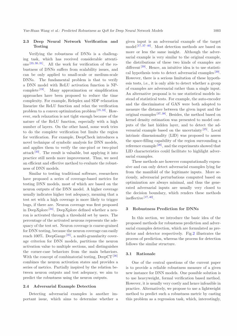
2.3 Deep Neural Network Verification andTesting
Verifying the robustness of DNNs is a challeng-
ing task, which has received considerable attenti-
ons [23, 30, 31]. All the work for verification of the ro-
bustness of DNNs suffers from scalability issues, and
can be only applied to small-scale or medium-scale
DNNs. The fundamental problem is that to verify
a DNN model with ReLU activation function is NP-
complete [19]. Many approximation or simplification
approaches have been proposed to reduce the time
complexity. For example, Releplex and SDP relaxation
linearize the ReLU function and relax the verification
problem to a convex optimization problem [19, 32]. How-
ever, such relaxation is not tight enough because of the
nature of the ReLU function, especially with a high
number of layers. On the other hand, some work tries
to do the complete verification but limits the region
for verification. For example, DeepCheck introduces a
novel technique of symbolic analysis for DNN models,
and applies them to verify the one-pixel or two-pixel
attack [33]. The result is valuable, but applying it into
practice still needs more improvement. Thus, we need
an efficient and effective method to evaluate the robust-
ness of DNN models.
Similar to testing traditional software, researchers
have proposed a series of coverage-based metrics for
testing DNN models, most of which are based on the
neuron outputs of the DNN model. A higher coverage
usually indicates higher test adequacy, meaning that a
test set with a high coverage is more likely to trigger
bugs, if there are. Neuron coverage was first proposed
in DeepXplore [34]. DeepXplore defined whether a neu-
ron is activated through a threshold set by users. The
percentage of the activated neurons represents the ade-
quacy of the test set. Neuron coverage is coarse-grained
for DNN testing, because the neuron coverage can easily
reach 100%. DeepGauge [35], a multi-granularity cover-
age criterion for DNN models, partitions the neuron
activation value to multiple sections, and distinguishes
the corner-case behaviors from the main behaviors.
With the concept of combinatorial testing, DeepCT [36]
combines the neuron activation states and provides a
series of metrics. Partially inspired by the relation be-
tween neuron outputs and test adequacy, we aim to
predict the robustness using the neuron outputs.
2.4 Adversarial Example Detection
Detecting adversarial examples is another im-
portant issue, which aims to determine whether a
given input is an adversarial example of the target
model [17, 37–40]. Most detection methods are based on
more or less the same insight. Although the adver-
sarial example is very similar to the original example,
the distributions of these two kinds of examples are
different [39]. Hence, an intuitive idea is to use statisti-
cal hypothesis tests to detect adversarial examples [39].
However, there is a serious limitation of these hypoth-
esis tests, i.e., it is only able to detect whether a group
of examples are adversarial rather than a single input.
An alternative proposal is to use statistical models in-
stead of statistical tests. For example, the auto-encoder
and the discriminator of GAN were both adopted to
measure the distance between the given input and the
original examples [37, 38]. Besides, the method based on
kernel density estimation was presented to model out-
puts of the last hidden layer, and to detect the ad-
versarial example based on the uncertainty [25]. Local
intrinsic dimensionality (LID) was proposed to assess
the space-filling capability of the region surrounding a
reference example [26], and the experiments showed that
LID characteristics could facilitate to highlight adver-
sarial examples.
These methods are however computationally expen-
sive and can only detect adversarial examples lying far
from the manifold of the legitimate inputs. More se-
riously, adversarial perturbations computed based on
optimization are always minimal, and thus the gene-
rated adversarial inputs are usually very closed to
the decision boundary, which renders these methods
ineffective [17, 40].
3 Robustness Prediction for DNNs
In this section, we introduce the basic idea of the
proposed methods for robustness prediction and adver-
sarial examples detection, which are formulated as pre-
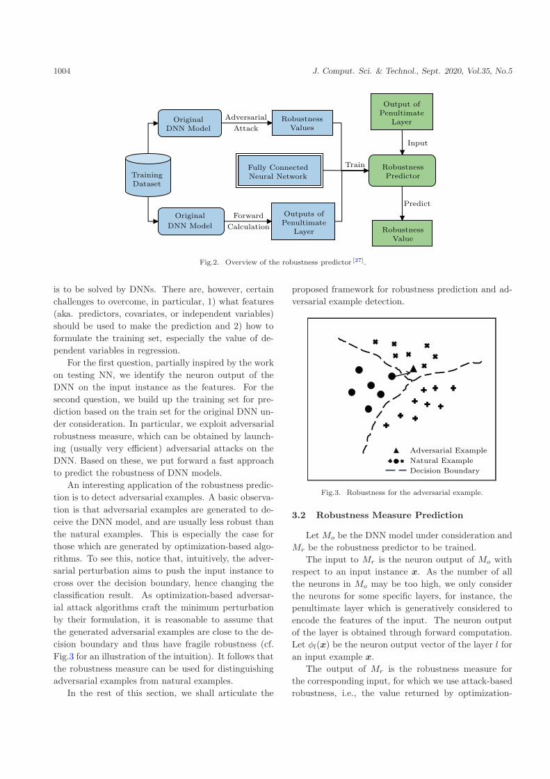
dictor and detector respectively. Fig.2 illustrates the
process of prediction, whereas the process for detection
follows the similar structure.
3.1 Rationale
One of the central questions of the current paper
is to provide a reliable robustness measure of a given
new instance for DNN models. One possible solution is
to use heavyweight, formal verification based method.
However, it is usually very costly and hence infeasible in
practice. Alternatively, we propose to use a lightweight
method to predict such a robustness metric by casting
this problem as a regression task, which, interestingly,
1004 J. Comput. Sci. & Technol., Sept. 2020, Vol.35, No.5
OriginalDNN Model
Adversarial
Attack
RobustnessValues
Output ofPenultimate
Layer
Input
Train
Predict
RobustnessValue
Outputs ofPenultimate
Layer
Forward
Calculation
Original
DNN Model
TrainingDataset
Fully ConnectedNeural Network
RobustnessPredictor
Fig.2. Overview of the robustness predictor [27].
is to be solved by DNNs. There are, however, certain
challenges to overcome, in particular, 1) what features
(aka. predictors, covariates, or independent variables)
should be used to make the prediction and 2) how to
formulate the training set, especially the value of de-
pendent variables in regression.
For the first question, partially inspired by the work
on testing NN, we identify the neuron output of the
DNN on the input instance as the features. For the
second question, we build up the training set for pre-
diction based on the train set for the original DNN un-
der consideration. In particular, we exploit adversarial
robustness measure, which can be obtained by launch-
ing (usually very efficient) adversarial attacks on the
DNN. Based on these, we put forward a fast approach
to predict the robustness of DNN models.
An interesting application of the robustness predic-
tion is to detect adversarial examples. A basic observa-
tion is that adversarial examples are generated to de-
ceive the DNN model, and are usually less robust than
the natural examples. This is especially the case for
those which are generated by optimization-based algo-
rithms. To see this, notice that, intuitively, the adver-
sarial perturbation aims to push the input instance to
cross over the decision boundary, hence changing the
classification result. As optimization-based adversar-
ial attack algorithms craft the minimum perturbation
by their formulation, it is reasonable to assume that
the generated adversarial examples are close to the de-
cision boundary and thus have fragile robustness (cf.
Fig.3 for an illustration of the intuition). It follows that
the robustness measure can be used for distinguishing
adversarial examples from natural examples.
In the rest of this section, we shall articulate the
proposed framework for robustness prediction and ad-
versarial example detection.
Adversarial Example
Natural Example
Decision Boundary
Fig.3. Robustness for the adversarial example.
3.2 Robustness Measure Prediction
Let Mo be the DNN model under consideration and
Mr be the robustness predictor to be trained.
The input to Mr is the neuron output of Mo with
respect to an input instance x. As the number of all
the neurons in Mo may be too high, we only consider
the neurons for some specific layers, for instance, the
penultimate layer which is generatively considered to
encode the features of the input. The neuron output
of the layer is obtained through forward computation.
Let φl(x) be the neuron output vector of the layer l for
an input example x.
The output of Mr is the robustness measure for
the corresponding input, for which we use attack-based
robustness, i.e., the value returned by optimization-

Yue-Huan Wang et al.: Predicted Robustness as QoS for Deep Neural Network Models 1005
based adversarial attacking algorithms for each input
instance. This problem deserves further discussions and
as a priori it is not clear why these adversarial attacking
algorithms provide a sensible estimate of the robust-
ness.
As in Subsection 2.2, a plethora of adversarial exam-
ple generation algorithms have been proposed, making
attacking DNNs as a routine task. A commonality of
most adversarial attack algorithms is to synthesize the
minimal perturbation that can fool the DNN model.
We hypothesize that these algorithms perform consis-
tently on this regard and design experiments to explore
the relation of different measures they generate. In
the experiment, we select three adversarial attack al-
gorithms, i.e., C&W, BIM, and Deepfool, to generate
the minimum perturbation as the respective robustness
measure of the DNN model. We analyze the corre-
lations among the three robustness measures via the
Pearson correlation coefficient (PCC) [41], which can il-
lustrate the linear correlation between two datasets (cf.
Subsection 4.1 for details).
Table 1 shows the experimental results, where we
use LeNet-5 and VGG-19 as the DNN models for classi-
fying the MNIST and CIFAR-10 datasets, respectively.
We can see that the robustness values calculated by
different adversarial attack algorithms are highly corre-
lated (in particular, all the PCC values are no less than
0.6). Therefore, it is reasonable to assume that these
quantities prescribe consistent and sound measures for
DNN robustness, which, from a practical point of view,
provide a valuable alternative for large-scale DNN mod-
els other than costly methods based on formal verifica-
tion.
Table 1. PCC of Attack-Based Robustness Measurements
DNN Model Measurement C&W Deepfool BIM
LeNet-5 (MNIST) C&W 1.00 0.86 0.92Deepfool 0.86 1.00 0.85BIM 0.92 0.85 1.00
VGG-19 (CIFAR-10) C&W 1.00 0.73 0.76Deepfool 0.73 1.00 0.60BIM 0.76 0.60 1.00
The training set for the robustness predictor can
then be collected as follows. Recall that the dataset
for Mo is composed by pairs of the form (xi, yi) for
the image example xi with the classification label yi.
The dataset for the robustness predictor Mr is thus
(φl(xi), ri), where φl(xi) is the neuron output vector
and ri is the robustness value.
For a given example xi, its robustness prediction is
given as:
r = Mr(φl(x)).
We note that training the DNN Mr is completed
offline and there is no overhead to collect new data
online. Moreover, during the training process of Mo,
practitioners can calculate the robustness values of all
the test examples to assess how robust Mo is.
3.3 Adversarial Example Detection
The detector is designed following the same frame-
work as the robustness predictor. The basic principle
is that we hypothesize that natural examples have a
higher degree of robustness than adversarial examples.
As a result, one can learn a threshold to separate them.
To this end, we use the neuron output from both
adversarial examples and natural examples to train the
detector model Md, for which we use the neurons of the
penultimate layer as the input of Md. For a new input
of the DNN model, Md outputs a score to indicate the
degree that the input is an adversarial example. For
training purposes, the score values of adversarial exam-
ples are set to be 0, and 1 for natural examples.
For a given input x, the score is computed as fol-
lows.
s = Md(φl(x)).
The lower the score is, the more likely that the input is
an adversarial example.
4 Evaluation
In this section, we evaluate the performance of our
approaches. We focus on the following four research
questions.
• RQ1 (Effectiveness and Efficiency of the
Predictor). Can the robustness predictor predict the
robustness effectively and efficiently?
• RQ2 (Applicability of the Predictor). Can the
robustness predictor be applied to DNN models with
different accuracies?
• RQ3 (Layer Selection). Does considering neuron
outputs from more layers improve the robustness pre-
dictor?
• RQ4 (Effectiveness of the Detector). Can the de-
tector detect adversarial examples effectively?
4.1 Experimental Setup
Datasets and DNN Models. We select four
well-adopted image classification datasets, MNIST [42],
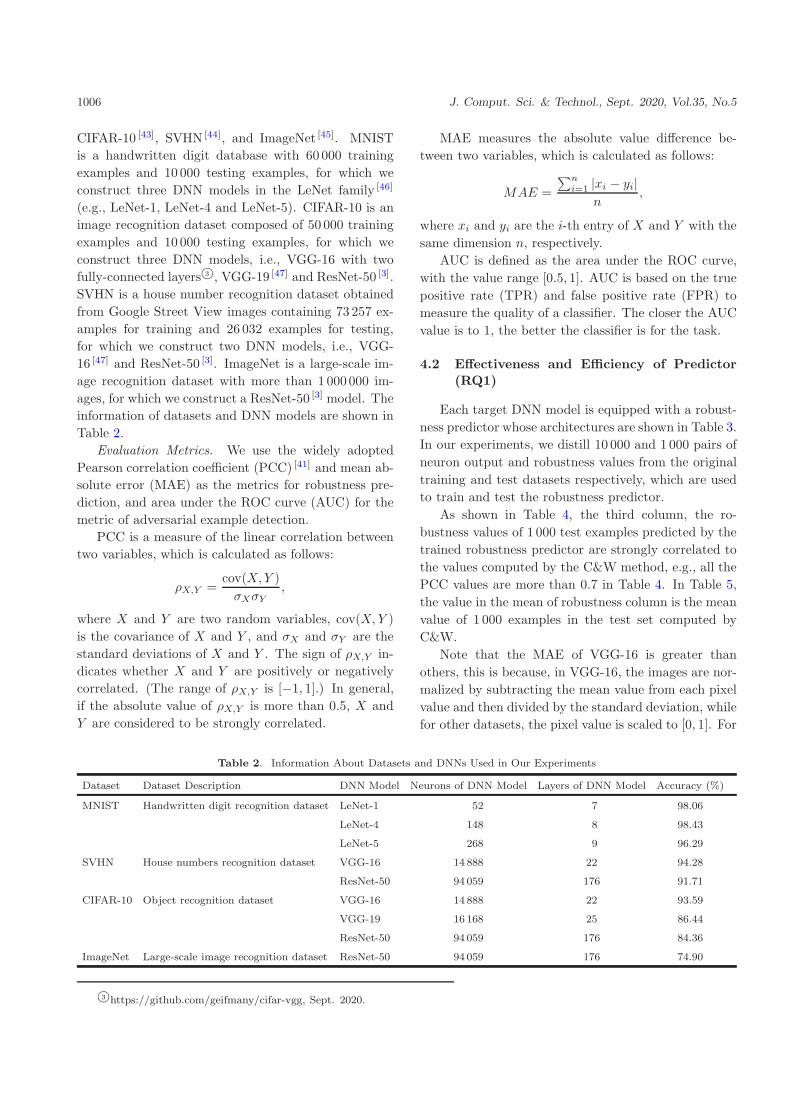
1006 J. Comput. Sci. & Technol., Sept. 2020, Vol.35, No.5
CIFAR-10 [43], SVHN [44], and ImageNet [45]. MNIST
is a handwritten digit database with 60 000 training
examples and 10 000 testing examples, for which we
construct three DNN models in the LeNet family [46]
(e.g., LeNet-1, LeNet-4 and LeNet-5). CIFAR-10 is an
image recognition dataset composed of 50 000 training
examples and 10 000 testing examples, for which we
construct three DNN models, i.e., VGG-16 with two
fully-connected layers 3○, VGG-19 [47] and ResNet-50 [3].
SVHN is a house number recognition dataset obtained
from Google Street View images containing 73 257 ex-
amples for training and 26 032 examples for testing,
for which we construct two DNN models, i.e., VGG-
16 [47] and ResNet-50 [3]. ImageNet is a large-scale im-
age recognition dataset with more than 1 000 000 im-
ages, for which we construct a ResNet-50 [3] model. The
information of datasets and DNN models are shown in
Table 2.
Evaluation Metrics. We use the widely adopted
Pearson correlation coefficient (PCC) [41] and mean ab-
solute error (MAE) as the metrics for robustness pre-
diction, and area under the ROC curve (AUC) for the
metric of adversarial example detection.
PCC is a measure of the linear correlation between
two variables, which is calculated as follows:
ρX,Y =cov(X,Y )
σXσY
,
where X and Y are two random variables, cov(X,Y )
is the covariance of X and Y , and σX and σY are the
standard deviations of X and Y . The sign of ρX,Y in-
dicates whether X and Y are positively or negatively
correlated. (The range of ρX,Y is [−1, 1].) In general,
if the absolute value of ρX,Y is more than 0.5, X and
Y are considered to be strongly correlated.
MAE measures the absolute value difference be-
tween two variables, which is calculated as follows:
MAE =
∑n
i=1 |xi − yi|
n,
where xi and yi are the i-th entry of X and Y with the
same dimension n, respectively.
AUC is defined as the area under the ROC curve,
with the value range [0.5, 1]. AUC is based on the true
positive rate (TPR) and false positive rate (FPR) to
measure the quality of a classifier. The closer the AUC
value is to 1, the better the classifier is for the task.
4.2 Effectiveness and Efficiency of Predictor
(RQ1)
Each target DNN model is equipped with a robust-
ness predictor whose architectures are shown in Table 3.
In our experiments, we distill 10 000 and 1 000 pairs of
neuron output and robustness values from the original
training and test datasets respectively, which are used
to train and test the robustness predictor.
As shown in Table 4, the third column, the ro-
bustness values of 1 000 test examples predicted by the
trained robustness predictor are strongly correlated to
the values computed by the C&W method, e.g., all the
PCC values are more than 0.7 in Table 4. In Table 5,
the value in the mean of robustness column is the mean
value of 1 000 examples in the test set computed by
C&W.
Note that the MAE of VGG-16 is greater than
others, this is because, in VGG-16, the images are nor-
malized by subtracting the mean value from each pixel
value and then divided by the standard deviation, while
for other datasets, the pixel value is scaled to [0, 1]. For
Table 2. Information About Datasets and DNNs Used in Our Experiments
Dataset Dataset Description DNN Model Neurons of DNN Model Layers of DNN Model Accuracy (%)
MNIST Handwritten digit recognition dataset LeNet-1 52 7 98.06
LeNet-4 148 8 98.43
LeNet-5 268 9 96.29
SVHN House numbers recognition dataset VGG-16 14 888 22 94.28
ResNet-50 94 059 176 91.71
CIFAR-10 Object recognition dataset VGG-16 14 888 22 93.59
VGG-19 16 168 25 86.44
ResNet-50 94 059 176 84.36
ImageNet Large-scale image recognition dataset ResNet-50 94 059 176 74.90
3○https://github.com/geifmany/cifar-vgg, Sept. 2020.

Yue-Huan Wang et al.: Predicted Robustness as QoS for Deep Neural Network Models 1007
Table 3. Architecture of Robustness Predictors
Dataset DNN Model Robustness Predictor
MNIST LeNet-1 588× 120× 84× 10× 1
LeNet-4 84× 120× 84× 10× 1
LeNet-5 84× 120× 84× 10× 1
CIFAR-10 VGG-16 512× 256× 256× 10× 1
VGG-19 512× 256× 256× 10× 1
ResNet-50 2 048× 256× 256× 10× 1
SVHN VGG-16 512× 256× 256× 10× 1
ResNet-50 512× 256× 256× 10× 1
the MNIST dataset, each image is 28× 28 resolution
and the pixel value is scaled to [0, 1]. The MAE results
show that the robustness predicted by the robustness
predictor is sufficiently accurate with 10%–30% errors.
These results show that the robustness predictor is ef-
fective in robustness prediction.
To further demonstrate the effectiveness of our ap-
proach, we consider three measures in literature which
are generally linked to robustness. These measures in-
clude confidence and two variants of surprise adequacy,
which are reasonable features for robustness prediction.
Confidence. A DNN-based classifier gives the proba-
bility of each class in the output layer. The class with
the maximum probability is the prescribed classification
result, which is also referred to as confidence, present-
ing how confident the DNN model is with regard to the
classification result. In general, high confidence means
that the DNN model would not change the classification
result easily, thereby in some sense confidence reflects
the robustness of the DNN model. It gives a convenient
robustness score as it comes from the normal classifica-
tion process without overhead.
Surprise Adequacy. Surprise adequacy (SA) is pro-
posed as a metric to measure the quality of the test
set for the DNN model [48], which provides users the
surprising degree of each test example. The surprising
degree is measured by the behavior difference of the
DNN model caused by the test example and the train-
ing data, which also indicates the robustness of the test
example. The DNN model is programmed by the train-
ing data and the behavior space caused by the training
data represents the learned logic inside the DNN model.
If an input example is more surprising, it causes more
behavior differences with the training data and is rarer
for the DNN model, making its classification result less
confident. Therefore an SA value also indicates the ro-
bustness value of a given example.
According to [48], the SA metric has two variants,
i.e., the likelihood-based surprise adequacy (LSA) and
the distance-based surprise adequacy (DSA). LSA [48]
estimates the probability density of a given input ex-
ample with the training data using kernel density esti-
Table 4. PCC for Predicting Robustness
Dataset DNN Model Robustness Measure
Robustness Predictor Confidence Regression LSA Regression DSA Regression
MNIST LeNet-1 0.92 0.81 0.22 0.61
LeNet-4 0.95 0.69 0.38 0.68
LeNet-5 0.95 0.86 0.10 0.08
CIFAR-10 VGG-16 0.83 0.36 0.63 0.69
VGG-19 0.90 0.31 0.53 0.73
ResNet-50 0.80 0.22 0.27 0.63
SVHN VGG-16 0.73 0.55 0.38 0.58
ResNet-50 0.78 0.48 0.07 0.01
Table 5. MAE for Predicting Robustness
Dataset DNN Model Robustness Measures Mean of
Robustness Predictor Confidence Regression LSA Regression DSA Regression Robustness
MNIST LeNet-1 0.15 0.24 0.39 0.31 1.30
LeNet-4 0.13 0.31 0.40 0.31 1.40
LeNet-5 0.13 0.23 0.46 0.46 1.37
CIFAR-10 VGG-16 0.20 0.38 0.29 0.26 0.93
VGG-19 0.07 0.77 0.13 0.10 0.32
ResNet-50 0.05 140.52 0.09 0.07 0.18
SVHN VGG-16 0.13 0.17 0.19 0.17 0.43
ResNet-50 0.05 0.08 0.10 0.10 0.16

1008 J. Comput. Sci. & Technol., Sept. 2020, Vol.35, No.5
mation (KDE), which is defined as follows:
g(x) =1
|αl(T )|
∑
xi∈T
K(αl(x)−αl(xi)),
where T is the training dataset, αl is the vector of acti-
vation values for the selected layer l, |αl(T )| is dimen-
sionality of the neuron outputs in the training set, and
K is the KDE function. LSA is defined as follows:
LSA(x) = − log(g(x)).
DSA [48] measures the surprising degree through the
Euclidean distance of the neuron output vectors gene-
rated by the a given input and examples in the train-
ing dataset, which provides the information about the
closeness of the given input to the decision boundary.
For a new test input x with the class C, let xi be the
nearest example of x with the same classification C,
and xj be the nearest example of xi with different clas-
sification other than C. disti is the Euclidean distance
of neuron outputs between x and xi, and distj is the
Euclidean distance of neuron outputs between xi and
xj . Then DSA is defined as
DSA(x) =disti
distj.
We adopt the polynomial regression to predict the
robustness with SA values as the input. Namely, we
vary polynomials of degrees up to n and select the one
with the best PCC value (in the experiment, we set
n = 10). Formally, we have
r = w1cn + w2c
n−1 + ...+ wnc1 + b,
where r represents the robustness value, c is the confi-
dence, DSA, or RSA, and w1, · · · , wn, b are the coeffi-
cients to be learned.
For LSA and DSA, as they compare the difference
between the test input and the training data, we can-
not use the examples in the original training dataset to
compute LSA and DSA. Hence, we use 5 000 test ex-
amples in the test set to compute LSA and DSA values
respectively as the training set to train the polynomial
regression model, and other 1 000 test examples as the
test set to evaluate the polynomial regression model.
Table 4 and Table 5 show the PCC and the MAE
results of the confidence regression model. The PCC
values of the robustness predictor are higher than those
of the confidence regression model, whereas the MAE
values of the robustness predictor are lower than those
of the confidence regression model. The results suggest
that the robustness predictor is superior to the confi-
dence regression model in predicting the robustness.
It is worth noticing that the MAE value of the
ResNet-50 model for the CIFAR-10 dataset is much
larger than others, because most of the confidence val-
ues are 1.0. This shows that the confidence has a weaker
relationship with the robustness. This is the inherent
defect of DNN models as they could prescribe a fragile
classification result very confidently.
For all the DNN models, the PCC values of the
robustness predictor are higher and the MAE values
are lower than both values of LSA and DSA, revealing
that the robustness predictor outperforms the regres-
sion models based on LSA and DSA.
Table 6 presents the time cost of obtaining the ro-
bustness values of 5 000 examples through the C&W
algorithm and the robustness predictor. The experi-
ment for the C&W algorithm is conducted with the
source code in [19]. We can see that the C&W algo-
rithm needs several hours, but the robustness predictor
only needs less than one second for the robustness cal-
culation of 5 000 examples. Most of the adversarial at-
tack techniques aim to get the minimum perturbation
by iterative algorithms, which means that the accurate
robustness result needs a certain number of iterations,
i.e., high time cost. When a new input comes, the at-
tack algorithm needs to execute again to calculate the
robustness value for this input. In contrast, the pro-
posed robustness predictor only needs a number of ro-
bustness values. The time cost of the training process
is offline, which does not have any influence during the
using process and can be accepted. When the new in-
put comes, the regression model predicts the robustness
based on the output from the penultimate layer of the
new input. The time cost mainly comes from the DNN
forward calculation, which is much less than the cost of
optimization-based adversarial attack algorithms. Ta-
ble 7 shows the memory and time cost of the robustness
predictor for LeNet-5 on three types of Android plat-
forms. The robustness predictor can conveniently be
applied on the mobile applications with the acceptable
running cost. In conclusion, the robustness predictor is
efficient for getting the robustness value.
For the ImageNet dataset, we train a robustness
predictor for a ResNet-50 model. Since the ImageNet
is a large-scale image dataset with 224× 224× 3 im-
ages and 1 000 classes, we increase the scale of the
training data for the robustness predictor to 100 000
instances of neuron outputs from the penultimate layer.
The architecture we design for the robustness predic-

Yue-Huan Wang et al.: Predicted Robustness as QoS for Deep Neural Network Models 1009
tor is a 9-layer fully connected neural network, with
2 048× 1 000× 2 048× 1 024× 512× 256× 128× 10× 1
neurons for each layer. Besides, we use the weights
between two layers with 2 048 and 1 000 neurons from
the original ResNet-50 model to be the weights between
the first layer and the second layer in the robustness
predictor and we use L1 norm regularization for train-
ing the robustness predictor. The results are shown
in Table 8. The robustness predictor achieves the re-
sult of PCC 0.67 and MAE 39.46. The MAE shows
the 34% additional errors with mean of robustness
116.64, which is the mean value of 1 000 test examples’
robustness computed by C&W. Compared with the
result of confidence regression of PCC 0.61 and MAE
43.32, the robustness predictor works well on the large-
scale dataset. For the surprise-adequacy regression, it
needs to compare the features of the test input and the
training dataset, which is impossible for the large-scale
ImageNet training dataset.
Table 6. Time Cost (s) of C&W Adversarial Attack Measureand Robustness Predictor
Dataset DNN Model C&W Robustness Predictor
MNIST LeNet-1 3 242.59 0.15
LeNet-4 3 441.25 0.16
LeNet-5 3 344.78 0.15
CIFAR-10 VGG-16 17 340.78 0.16
VGG-19 13 116.62 0.16
ResNet-50 44 129.12 0.16
SVHN VGG-16 1 995.18 0.07
ResNet-50 4 376.64 0.07
Table 7. Memory (MB) and Time Cost (ms) of RobustnessPredictor for LeNet-5 on Android Platforms
Type Memory Time Cost
Galaxy Nexus 31.38 21
Nexus 6 43.52 12
Pixel 44.48 10
Table 8. Results for ImageNet Dataset
Robsutness Measure PCC MAE Mean of Robustness
Robustness predictor 0.67 39.46 116.64
Confidence regression 0.61 43.32 116.64
As for the design of the robustness predictor, we
suggest referring to the last few fully connected layers
of the target DNN model. For the ResNet-50 model on
ImageNet dataset, we use the last two layers in ResNet-
50 as the first two layers to leverage the representations
learnt by the target model. Since the dimension of rep-
resentations of ResNet-50 on ImageNet is much higher
than that on small datasets, we add more layers for di-
mension reduction and representation learning for the
final regression task. During the practical usage of the
robustness predictor for other datasets, users could first
try the architecture of fully connected layers in the tar-
get DNN model, and then add layers for further dimen-
sion reduction and representation learning. According
to our research, the predictor should not require a neu-
ral network with more than 10 layers.
Answer to RQ1. The robustness predictor can pre-
dict the robustness of individual input instances effec-
tively and efficiently.
4.3 Application Range of Predictor (RQ2)
Since users may have different skills and experiences
in training DNN models, not all the models can be
trained well to reach a high accuracy. We measure
the mean robustness value of 1 000 examples in the
MNIST test set for five LeNet-5 models with accura-
cies of 75.60%, 80.49%, 85.47%, 90.07%, and 95.29%,
respectively. The results are shown in Fig.4.
75.60 80.49 85.47 90.07 95.29
Accuracy (%)
1.40
1.45
1.50
1.55
1.60
1.65
1.70
1.75
1.80
1.85
1.90
Mean V
alu
e o
f R
obust
ness
Fig.4. DNN models’ robustness with different accuracies [27].
In addition to the MNIST dataset, we also train
three VGG-16 models for the CIFAR-10 dataset, with
accuracies of 71.71%, 82.16%, and 93.59% respectively.
We observe that, for the same dataset and layer archi-
tecture, DNN models with different accuracies tend to
have different performance on the robustness, with the
same result for the CIFAR-10 dataset with the mean ro-
bustness values of 0.96, 0.96 and 0.93 for the accuracies
of 71.71%, 82.16% and 93.59%, respectively.

1010 J. Comput. Sci. & Technol., Sept. 2020, Vol.35, No.5
We next examine whether the robustness predictor
is effective for DNN models with different accuracies.
For the evaluation, as before, we compare the result
of the robustness predictor with those of confidence,
LSA, and DSA on DNN models. Fig.5 and Fig.6 show
the evaluation results, where RP, CR, LSA and DSA
standard for robustness predictor, confidence regres-
sion, LSA and DSA respectively.
For PCC, the robustness predictor obtains the val-
ues of no less than 0.9 for the MNIST dataset and no
less than 0.7 for the CIFAR-10 dataset. For MAE, the
robustness predictor achieves 0.10–0.17 and 0.20–0.22
for the MNIST and CIFAR-10 datasets, respectively.
Both confirm the efficacy of our approach in handling
models of different accuracies, and its superiority over
other methods.
Answer to RQ2. The robustness predictor can be
applied to DNN models with different accuracies.
4.4 Layer Selection (RQ3)
Using the neuron output from the penultimate layer
to train the robustness predictor is based on our intu-
ition that the features in the deeper layers are more
useful. However, it is important to study the impact
of the selection of layers on the robustness predictor.
To this end, we add neuron output from other layers to
train the robustness predictor and compute the PCC
and MAE results. In the experiment, we use three DNN
models, LeNet-5 for classifying the MNIST dataset,
VGG-16 and ResNet-50 for classifying the CIFAR-10
dataset. As the number of neurons in some layers may
be too large, we randomly select 100 neurons. (If there
75.60 80.49 85.47 90.07 95.29
Accuracy (%)
0.0
0.1
0.2
0.3
0.4
0.5
0.6
0.7
0.8
0.9
1.0
PC
C
0.0
0.1
0.2
0.3
0.4
0.5
0.6
0.7
0.8
0.9
1.0
PC
C
RP CR LSA DSA
71.71 82.16 93.59
Accuracy (%)
RP
CR
LSA
DSA
Fig.5. PCC results of DNN models with different accuracies [27]. (a) MNIST. (b) CIFAR-10.
75.60 80.49 85.47 90.07 95.29
Accuracy (%)
0.0
0.1
0.2
0.3
0.4
0.5
0.6
0.7
MA
E
RPCR
LSADSA
71.71 82.16 93.59
Accuracy (%)
0.0
0.1
0.2
0.3
0.4
0.5
0.6
0.7
MA
E
RPCR
LSADSA
Fig.6. MAE results of DNN models with different accuracies [27]. (a) MNIST. (b) CIFAR-10.

Yue-Huan Wang et al.: Predicted Robustness as QoS for Deep Neural Network Models 1011
are no more than 100 neurons for a layer, all will be
included.) As the input data becomes more compli-
cated, we also add some layers to the robustness pre-
dictor to improve its capacity. Specifically, we grad-
ually add the neuron outputs from dense 2, pooling 2
and pooling 1 of LeNet-5 and the neuron outputs from
pooling 5, pooling 4 and pooling 3 of VGG-16, add 16,
add 15 and add 14 of ResNet-50 to the training data
for the robustness predictor. For VGG-16, we choose
the pooling layers, which are the last layers of the con-
volutional blocks. For ResNet-50, we choose the add
layers, which are last layers of the residual blocks. As
for the architecture, we use 120× 100× 100× 84× 10
fully connected layers for the robustness predictor of
LeNet-5 and 256× 256× 256× 256× 10 fully connected
layers for that of VGG-16 and ResNet-50. The results
are shown in Table 9, Table 10 and Table 11. No sub-
stantial difference is observed for both PCC and MAE.
This suggests that adding extra neuron output from
other layer may not further improve the performance
of the robustness predictor. Namely, considering the
neuron output from the penultimate layer gives suffi-
cient features for the robustness prediction.
Answer to RQ3. There is no significant improve-
ment for the robustness predictor by adding neuron
outputs from other layers.
Table 9. Result of Layer Selection on MNIST
Layer PCC MAE
Penultimate 0.95 0.13
Penultimate, dense 2 0.96 0.12
Penultimate, dense 2, pooling 2 0.96 0.13
Penultimate, dense 2, pooling 2, pooling 1 0.95 0.13
Table 10. Result of Layer Selection for VGG-16 on CIFAR-10
Layer PCC MAE
Penultimate 0.83 0.20
Penultimate, pooling 5 0.83 0.20
Penultimate, pooling 5, pooling 4 0.81 0.21
Penultimate, pooling 5, pooling 4, pooling 3 0.80 0.22
Table 11. Result of Layer Selection for ResNet-50 on CIFAR-10
Layer PCC MAE
Penultimate, pooling 5 0.77 0.06
Penultimate, add 16, add 15 0.79 0.06
Penultimate, add 16, add 15, add 14 0.79 0.06
4.5 Effectiveness of Detector (RQ4)
To evaluate the effectiveness of the adversarial ex-
ample detection, we compare the proposed detector
with two state-of-the-art detection methods based on
kernel density (KD) and local intrinsic dimensionality
(LID), respectively.
We select six DNN models (LeNet-4 and LeNet-5 for
the MNIST dataset, VGG-16 and ResNet-50 for both
SVHN and CIFAR-10 datasets) for evaluation. Follow-
ing the experimental setting [26], the logistic regression
detectors of KD and LID are trained by the scores of
adversarial examples generated by FGSM. For the de-
tector in our approach, we use the scores of adversarial
examples generated by C&W. Up to 1 000 adversarial
examples generated by FGSM, C&W, BIM and JSMA
respectively are used as the test set. We compare the
AUC results of the proposed detector with those of KD-
and LID-based detectors as shown in Table 12.
Table 12. AUC (%) Results for Detecting Adversarial Examples
Dataset DNN Model Detector Adversarial Attack
FGSM C&W BIM JSMA
MNIST LeNet-4 KD 81.97 97.52 90.91 98.52
LID 89.12 99.69 98.36 99.06
Ours 93.21 99.65 96.40 99.08
LeNet-5 KD 72.70 89.86 75.65 94.61
LID 78.68 97.78 92.01 93.26
Ours 91.32 98.80 95.97 97.73
SVHN VGG-16 KD 79.31 85.45 79.15 85.95
LID 70.54 84.45 73.89 83.84
Ours 78.20 97.63 82.76 97.43
ResNet-50 KD 57.41 61.67 57.62 59.57
LID 79.90 85.30 77.88 71.93
Ours 78.18 92.85 82.39 92.77
CIFAR-10 VGG-16 KD 72.37 98.02 91.79 98.40
LID 74.78 98.32 91.24 98.63
Ours 72.82 98.44 95.70 98.78
ResNet-50 KD 53.13 69.86 53.35 68.31
LID 75.46 76.85 68.94 80.70
Ours 66.13 97.86 71.90 94.30
We can see that the proposed detector obtains bet-
ter performance than KD and LID detectors for C&W,
BIM and JSMA, which are based on the optimization
algorithms, on SVHN and CIFAR-10 datasets. For
LeNet-5, the proposed detector outperforms the other
methods for adversarial examples generated by the four
adversarial attacks, the same for LeNet-4 except for
BIM. Based on the experimental results, we conclude

1012 J. Comput. Sci. & Technol., Sept. 2020, Vol.35, No.5
that the proposed detector works effectively for detect-
ing adversarial examples generated by those optimiza-
tion algorithms.
Moreover, although the proposed detector has a
weaker effect on the FGSM attack, it is still mean-
ingful in detecting adversarial examples. Adversarial
examples generated by FGSM are usually easy to de-
tect, since the perturbation is relatively obvious, while
adversarial examples generated by the optimization al-
gorithms with imperceptible perturbation are difficult
to detect, which is the strength of our approach.
Answer to RQ4. The detector can detect adversarial
examples effectively.
4.6 Threats of Validity
In this subsection, we analyze threats to internal,
external and construct validity of our work.
The selection of the datasets and the DNN models
may externally threaten the validity of our evaluations.
For this problem, we choose three popular datasets, in-
cluding MNIST, CIFAR-10, and SVHN, and six state-
of-the-art DNN models, including LeNet-1, LeNet-4,
LeNet-5, VGG-16, VGG-19, and ResNet-50, as the ex-
perimental subjects. The datasets and the DNN mod-
els are diverse and representative for our experiments
to draw the conclusions. The implementation in our
experiments may also threaten the external validity of
our conclusions. We depend on the widely used Python
libraries, including Numpy, Sklearn, and Scipy to im-
plement our code for experiments.
The internal threat of the validity might come from
that we need a white-box DNN model for our ap-
proaches. Both the robustness predictor and the detec-
tor for detecting adversarial examples need the neuron
outputs inside the target DNN model as the training
data, which narrows the application range of our ap-
proaches. Usually, our approaches are used by users,
who provide the DNN models. The predictor and the
detector can be trained during the training process of
the target DNN model and used as the auxiliary tools.
Moreover, the robustness predictor is also a DNN-based
model; therefore it would also suffer from the adversar-
ial attack. Note that we provide the robustness pre-
dictor as the quality of service of the DNN model and
strive to make the robustness prediction convenient to
use and less costly. In practice, the robustness predic-
tor can be used in at least two ways. First, it predicts
the robustness value as the quality measurement dur-
ing the training process to, for instance, obtain a better
DNN model. Second, it can be deployed as a part of
the target DNN model to indicate the robustness of the
prediction for a new input instance. Usually users are
harder to acquire the internal neuron output of the tar-
get DNN model; thus it would be much more difficult
to synthesize the adversarial example for the robustness
predictor.
As for the threat of construction validity, the met-
rics for evaluating the experimental results are impor-
tant. We use PCC to measure the correlation between
the results predicted by the regression model and the
robustness values computed by the C&W attack, which
is commonly applied to measure the linear correlation
in, for instance, statistics and data mining. We use
MAE to measure the absolute error between the pre-
diction results and the robustness values, which is also
a generic measurement for the numerical difference in
machine learning research. We use AUC to measure the
effectiveness of detecting adversarial examples, which is
standard for comparison between classifiers in the ma-
chine learning.
5 Conclusions
In this paper, we proposed a fast robustness pre-
dictor, which is to predict a robustness measure for a
new input example of DNN-based classifiers. The ro-
bustness predictor can be co-trained with the classifier.
The lightweight feature of the approach makes it feasi-
ble to deploy on resource-constrained platforms such as
mobile devices. Based on the framework of the robust-
ness predictor, we also devised a detector for adversar-
ial examples generated by optimization-based attacks.
The experimental results showed the effectiveness and
efficiency of the proposed robustness predictor and ad-
versarial example detector.
In this paper, we only considered one type of per-
turbation, the L2 norm distance metric, while other
robustness properties, such as light change, image ro-
tation and so on, are still expected to be considered.
Towards the different forms of the perturbation, neu-
ron output solely may not be enough; extra informa-
tion, such as the neuron positions in the DNN model
may be in need. These deserve further investigation.
Furthermore, since we are able to use the neuron out-
put and the DNN structure to predict the robustness
of DNN models, it is conceivable that we may infer
some information about DNN interpretation along this
avenue. Since we only evaluated the proposed predic-
tor on CNN models, another direction is to extend the
Yue-Huan Wang et al.: Predicted Robustness as QoS for Deep Neural Network Models 1013
scope of our approach to other types of DNN models,
such as classic DNN and RNN models.
References
[1] Andor D, Alberti C, Weiss D, Severyn A, Presta A,
Ganchev K, Petrov S, Collins M. Globally normalized
transition-based neural networks. arXiv:1603.06042, 2016.
https://arxiv.org/abs/1603.06042, June 2020.
[2] Hinton G, Deng L, Yu D, Dahl G, Mohamed A, Jaitly N, Se-
nior A, Vanhoucke V, Nguyen P, Kingsbury B. Deep neural
networks for acoustic modeling in speech recognition: The
shared views of four research groups. IEEE Signal Process-
ing Magazine, 2012, 29(6): 82-97.
[3] He K, Zhang X, Ren S, Sun J. Deep residual learning for
image recognition. In Proc. the IEEE Conference on Com-
puter Vision and Pattern Recognition, June 2016, pp.770-
778.
[4] Wang X, Huang C, Yao L, Benatallah B, Dong M. A survey
on expert recommendation in community question answer-
ing. Journal of Computer Science and Technology, 2018,
33(4): 625-653.
[5] Liu Q, Zhao H K, Wu L, Li Z, Chen E H. Illuminating rec-
ommendation by understanding the explicit item relations.
Journal of Computer Science and Technology, 2018, 33(4):
739-755.
[6] Silver D, Huang A, Maddison C J et al. Mastering the game
of Go with deep neural networks and tree search. Nature,
2016, 529(7587): 484-489.
[7] Ameur H, Jamoussi S, Hamadou A B. A new method for
sentiment analysis using contextual auto-encoders. Journal
of Computer Science and Technology, 2018, 33(6): 1307-
1319.
[8] Bojarski M, Testa D D, Dworakowski D et al. End to
end learning for self-driving cars. arXiv:1604.07316, 2016.
https://arxiv.org/abs/1604.07316, June 2020.
[9] Esteva A, Kuprel B, Novoa R A, Ko J, Swetter S M, Blau H
M, Thrun S. Dermatologist-level classification of skin can-
cer with deep neural networks. Nature, 2017, 542(7639):
115-118.
[10] Yuan Z, Lu Y, Wang Z, Xue Y. Droid-Sec: Deep learning
in Android malware detection. ACM SIGCOMM Computer
Communication Review, 2014, 44(4): 371-372.
[11] Li Z, Ma X, Xu C, Xu J, Cao C, Lu J. Operational cali-
bration: Debugging confidence errors for DNNs in the field.
arXiv:1910.02352, 2019. https://arxiv.org/abs/1910.02352,
Sept. 2020.
[12] Li Z, Ma X, Xu C, Cao C, Xu J, Lu J. Boosting opera-
tional DNN testing efficiency through conditioning. In Proc.
the 27th ACM Joint Meeting on European Software Engi-
neering Conference and Symposium on the Foundations of
Software Engineering, August 2019, pp.499-509.
[13] LeCun Y, Bengio Y, Hinton G. Deep Learning. MIT Press,
2016.
[14] Burrell J. How the machine ‘thinks’: Understanding opa-
city in machine learning algorithms. Big Data & Society,
2016, 3(1): Article No. 2053951715622512.
[15] Goodfellow I J, Shlens J, Szegedy C. Explaining and
harnessing adversarial examples. arXiv:1412.6572, 2014.
https://arxiv.org/abs/1412.6572, June 2020.
[16] Moosavi-Dezfooli S, Fawzi A, Frossard P. DeepFool: A sim-
ple and accurate method to fool deep neural networks. In
Proc. IEEE Conference on Computer Vision and Pattern
Recognition, June 2016, pp.2574-2582.
[17] Carlini N, Wagner D. Adversarial examples are not easily
detected: Bypassing ten detection methods. In Proc. the
10th ACM Workshop on Artificial Intelligence and Secu-
rity, November 2017, pp.3-14.
[18] Athalye A, Carlini N, Wagner D. Obfuscated gradi-
ents give a false sense of security: Circumventing de-
fenses to adversarial examples. arXiv:1802.00420, 2018.
https://arxiv.org/abs/1802.00420, June 2020.
[19] Katz G, Barrett C, Dill D L, Julian K, Kochenderfer M J.
Reluplex: An efficient SMT solver for verifying deep neu-
ral networks. In Proc. the 29th International Conference on
Computer Aided Verification, July 2017, pp.97-117.
[20] Bastani O, Ioannou Y, Lampropoulos L, Vytiniotis D, Nori
A, Criminisi A. Measuring neural net robustness with con-
straints. In Proc. the Annual Conference on Neural Infor-
mation Processing Systems, December 2016, pp.2613-2621.
[21] Hendrycks D, Gimpel K. A baseline for detecting misclas-
sified and out-of-distribution examples in neural networks.
arXiv:1610.02136, 2016. https://arxiv.org/abs/1610.02136,
June 2020.
[22] Weng T, Zhang H, Chen H, Song Z, Hsieh C, Boning D,
Dhillon I S, Daniel L. Towards fast computation of certi-
fied robustness for ReLU networks. arXiv:1804.09699, 2018.
https://arxiv.org/abs/1804.09699, June 2020.
[23] Singh G, Gehr T, Puschel M, Vechev M. An abstract do-
main for certifying neural networks. Proceedings of the
ACM on Programming Languages, 2019, 3(POPL): Arti-
cle No. 41.
[24] Carlini N, Wagner D. Towards evaluating the robustness of
neural networks. In Proc. the 2017 IEEE Symposium on
Security and Privacy, May 2017, pp.39-57.
[25] Feinman R, Curtin R R, Shintre S, Gardner A B. Detecting
adversarial samples from artifacts. arXiv:1703.00410, 2017.
https://arxiv.org/abs/1703.00410, June 2020.
[26] Ma X, Li B, Wang Y, Erfani S M, Wijewickrema
S, Schoenebeck G, Song D, Houle M E, Bailey J.
Characterizing adversarial subspaces using local intrinsic
dimensionality. arXiv:1801.02613, 2018. https://arxiv.or-
g/abs/1801.02613, June 2020.
[27] Wang Y, Li Z, Xu J, Yu P, Ma X. Fast robustness predic-
tion for deep neural network. In Proc. the 11th Asia-Pacific
Symposium on Internetware, Oct. 2019.
[28] Kurakin A, Goodfellow I, Bengio S. Adversarial ex-
amples in the physical world. arXiv:1607.02533, 2016.
https://arxiv.org/abs/1607.02533, June 2020.
[29] Papernot N, McDaniel P, Jha S, Fredrikson M, Celik Z B,
Swami A. The limitations of deep learning in adversarial
settings. In Proc. the 2016 IEEE European Symposium on
Security and Privacy, March 2016, pp.372-387.

1014 J. Comput. Sci. & Technol., Sept. 2020, Vol.35, No.5
[30] Huang X, Kroening D, Kwiatkowska M, Ruan W, Sun Y,
Thamo E, Wu M, Yi X. Safety and trustworthiness of
deep neural networks: A survey. arXiv:1812.08342, 2018.
https://arxiv.org/abs/1812.08342, June 2020.
[31] Huang X, Kwiatkowska M, Wang S, Wu M. Safety veri-
fication of deep neural networks. In Proc. the 29th Inter-
national Conference on Computer Aided Verification, July
2017, pp.3-29.
[32] Wong E, Kolter J Z. Provable defenses against adversar-
ial examples via the convex outer adversarial polytope.
arXiv:1711.00851, 2017. https://arxiv.org/abs/1711.00851,
June 2020.
[33] Gopinath D, Pasareanu C S, Wang K, Zhang M, Khurshid
S. Symbolic execution for attribution and attack synthesis
in neural networks. In Proc. the 41st IEEE/ACM Inter-
national Conference on Software Engineering, May 2019,
pp.282-283.
[34] Pei K, Cao Y, Yang J, Jana S. DeepXplore: Automated
whitebox testing of deep learning systems. In Proc. the
26th Symposium on Operating Systems Principles, Octo-
ber 2017, pp.1-18.
[35] Ma L, Juefei-Xu F, Zhang F et al. DeepGauge: Multi-
granularity testing criteria for deep learning systems. In
Proc. the 33rd ACM/IEEE International Conference on
Automated Software Engineering, September 2018, pp.120-
131.
[36] Ma L, Zhang F, Xue M, Li B, Liu Y, Zhao J, Wang
Y. Combinatorial testing for deep learning systems.
arXiv:1806.07723, 2018. https://arxiv.org/abs/1806.07723,
June 2020.
[37] Zong B, Song Q, Min M, Cheng W, Lumezanu C, Cho
D, Chen H. Deep autoencoding Gaussian mixture model
for unsupervised anomaly detection. In Proc. International
Conference on Learning Representations, February 2018.
[38] Santhanam G K, Grnarova P. Defending against adversar-
ial attacks by leveraging an entire GAN. arXiv:1805.10652,
2018. https://arxiv.org/abs/1805.10652, June 2020.
[39] Grosse K, Manoharan P, Papernot N, Backes M, McDaniel
P. On the (statistical) detection of adversarial examples.
arXiv:1702.06280, 2017. https://arxiv.org/abs/1702.06280,
June 2020.
[40] Xu W, Evans D, Qi Y. Feature squeezing: Detecting adver-
sarial examples in deep neural networks. arXiv:1704.01155,
2017. https://arxiv.org/abs/1704.01155, June 2020.
[41] Benesty J, Chen J, Huang Y, Cohen I. Pearson correlation
coefficient. In Noise Reduction in Speech Processing, Co-
hen I, Huang Y, Chen J, Benesty J (eds.), Springer, 2009,
pp.1-4.
[42] LeCun L, Boser B, Denker J S, Henderson D, Howard R E,
Hubbard W, Jackel L D. Backpropagation applied to hand-
written zip code recognition. Neural Computation, 1989,
1(4): 541-551.
[43] Krizhevsky A. Learning multiple layers of features from
tiny images. Technical Report, University of Toronto,
2009. http://www.cs.toronto.edu/∼kriz/learning-features-
2009-TR.pdf, June 2020.
[44] Netzer Y, Wang T, Coates A, Bissacco A, Wu B, Ng A Y.
Reading digits in natural images with unsupervised feature
learning. In Proc. the NIPS Workshop on Deep Learning
and Unsupervised Feature Learning, Dec. 2011.
[45] Deng J, Dong W, Socher R, Li L J, Li K, Li F F. ImageNet:
A large-scale hierarchical image database. In Proc. the 2009
IEEE Conference on Computer Vision and Pattern Recog-
nition, June 2009, pp.248-255.
[46] LeCun L, Bottou L, Bengio Y, Haffner P. Gradient-based
learning applied to document recognition. Proceedings of
the IEEE, 1998, 86(11): 2278-2324.
[47] Simonyan K, Zisserman A. Very deep convolutional net-
works for large-scale image recognition. arXiv:1409.1556,
2014. https://arxiv.org/abs/1409.1556, June 2020.
[48] Kim J, Feldt R, Yoo S. Guiding deep learning system test-
ing using surprise adequacy. In Proc. the 41st International
Conference on Software Engineering, May 2019, pp.1039-
1049.
Yue-Huan Wang is currently
pursuing her Master’s degree with
the State Key Laboratory for Novel
Software Technology and Department
of Computer Science and Technology
at Nanjing University, Nanjing. Her
research interests include quality assur-
ance for machine learning models used
as software components.
Ze-Nan Li is currently a student
with the State Key Laboratory for Novel
Software Technology and Department
of Computer Science and Technology
at Nanjing University, Nanjing. His
research interests include quality as-
surance for machine learning models
used as software components and fast
algorithms for large scale machine learning problems.
Jing-Wei Xu is an assistant pro-
fessor with the State Key Laboratory
for Novel Software Technology and
Department of Computer Science and
Technology at Nanjing University,
Nanjing. He received his M.Sc. and
Ph.D. degrees from Nanjing University
in 2012 and 2017, both in computer
science. His research interests are quality assurance for
machine learning models, representation understanding,
and deep learning. He has published many referred papers
in both international software engineering and machine
learning conferences. He is a member of CCF and ACM.

Yue-Huan Wang et al.: Predicted Robustness as QoS for Deep Neural Network Models 1015
Ping Yu received her Ph.D. degree
in computer science and technology in
2008 from Nanjing University, Nanjing.
She is an associate professor with
the State Key Laboratory for Novel
Software Technology and Department
of Computer Science and Technology
at Nanjing University, Nanjing. Her
research interests include big data software engineering,
software evolution and cloud computing. She is a member
of CCF.
Taolue Chen received his B.S.
and M.S. degrees from the Nanjing
University, Nanjing, both in computer
science. He was a junior researcher at
the Centrum Wiskunde & Informatica
(CWI) and acquired his Ph.D. degree
in computer science from the Vrije Uni-
versiteit Amsterdam, The Netherlands.
He is currently a senior lecturer at the Department of
Computer Science, University of Surrey, Guiford. His
research interests include formal verification and synthesis,
program analysis, software security, software engineering
and machine learning. He has co-authored about 100
peer-reviewed conference and journal papers, and has
served as a technical program committee member for
various international conferences.
Xiao-Xing Ma is currently a full
professor with the State Key Labo-
ratory for Novel Software Technology
and Department of Computer Science
and Technology at Nanjing University,
Nanjing. From the same university, he
received his Ph.D. degree in computer
science in 2003. His research interests
include self-adaptive software systems, software architec-
tures, and quality assurance for machine learning models
used as software components. He co-authored over 100
peer-reviewed papers and served in technical program
committees of various international software engineering
conferences. He is a member of CCF, ACM and IEEE.