precision medicine: lecture 15 multiple utilities

Precision Medicine: Lecture 15Multiple Utilities

Michael R. Kosorok,Nikki L. B. Freeman and Owen E. Leete

Department of BiostatisticsGillings School of Global Public Health

University of North Carolina at Chapel Hill

Fall, 2019

Outline

Incorporating patient preferences

Estimation and Optimization of Composite Outcomes

Michael R. Kosorok, Nikki L. B. Freeman and Owen E. Leete 2/ 52

Shared decision making

I So far we have focused on DTRs that tailor treatments toindividual patient characteristics.

I Patient characteristics may include clinical information aswell as patient preferences.

I Recall that an optimal DTR maximizes the mean of apre-specified clinical outcome if it is applied to all patientsin a population of interest.

I While this definition of optimality is mathematicallyconvenient, it does not directly allow for shared decisionmaking where patient preferences are integrated into thedecision process.


Why including patient preferences into DTRconstruction is important

I Including patient preferences in treatment selection in amathematically rigorous way is important.

I First, it facilitates ‘patient-centered care’ in whichpatients play a key role in decision making and theevaluation of their own outcomes.

I Second, it offers a principled means for matching patientpreferences to an optimal treatment based on potentiallycomplex outcome profiles.


Patient preference elicitation

I Eliciting patient preferences is not necessarilystraightforward.

I For example, it would be convenient if patients couldchoose parameters indexing a composite outcome.However, without specialized training for the patients, thisis not feasible.

I An alternative approach is to administer a questionnairepopulated with items that are accessible to a patient in adomain context yet are informative about preferences inthe outcome space.

I Butler, Laber, Davis, and Kosorok (2018) incorporate thislatter approach to derive a preference-sensitive optimalDTR for each patient. We will explore their proposedmethodology in detail.


Setup and notation

I Observed data {Wi ,Xi ,Ai ,Yi ,Zi}ni=1 comprises nindependent and identically distributed tuples(W,X,A,Y ,Z ) where

I W ∈ {0, 1}p denotes answers to items in a preferencequestionnaire,

I X ∈ Rm denotes pre-treatment patient covariates,

I A ∈ {−1, 1} denotes the assigned treatment,

I Y ,Z ∈ R denote outcomes of interest, coded so that highervalues are better.

I A DTR is denoted by π : dom W × dom X→ dom A.


Optimal DTR

To define an optimal DTR,

I Assume that each individual in the pouplation has a latentpreference, H ∈ R, that indexes a utility functionU(y , z ; h).

I Assume that the utility function induces an ordering ondom Y × dom Z so that a patient with preference H = hwould prefer outcomes (y , z) to (y ′, z ′) ifU(y , z ; h) ≥ U(y ′, z ′; h).


Optimal DTR (cont.)

I Let Y ∗(a) and Z ∗(a) denote the potential outcomesunder treatments a ∈ {−1, 1} so that U{Y ∗(a),Z ∗(a)} isthe potential utility function under treatment a.

I Define the potential utility as

VU(π) = E[ ∑

a∈{−1,1}

U{Y ∗(a),Z ∗(a);H}I (π(W,X) = a)

]where the expectation is taken with respect to the jointdistribution of {X,W,H ,A,Y ∗(0),Y ∗(1),Z ∗(0),Z ∗(1)}.

I The optimal DTR, πoptU satisfies

VU(πoptU ) ≥ VU(π) for all π.


Form of the utility

I Assume the utility has the form

U(y , z ; h) = Φ(h)y + {1− Φ(h)}z

where Φ(·) denotes the cumulative distribution functionfor a standard normal random variable.

I Interpretation: A patient with preference h caresΦ(h)/(1− Φ(h)) more about Y than Z .

I Linear utility is a common assumption in multiobjectiveoptimization, however the assumption of a constant gainin utility per unit increase in outcome may not bereasonable in some contexts.


The optimal DTR for any rational utility can beexpressed as the optimal DTR for some linear utility

I A rational utility will always prefer a treatment that isbetter on both outcomes to one that is worse on bothoutcomes.

I Butler et al. (2018) prove that the DTR for any rationalutility may be expressed as the optimal DTR for somelinear utility function.

I To state this formally, define the following

RZ (w, x) = {Z∗(1)|W = w,X = x} − {Z∗(−1)|W = w,X = x}RY (w, x) = {Y ∗(1)|W = w,X = x} − {Y ∗(−1)|W = w,X = x},RU(w, x) = {U{Y ∗(1),Z∗(1);H}|W = w,X = x}

− {U{Y ∗(−1),Z∗(−1);H}|W = w,X = x}.

I Note, it can be shown that πoptU (w, x) = sign{RU(w, x)}


The optimal DTR for any rational utility is theoptimal DTR for some linear utility (formally)

Lemma (2.1)Assume that max{RU(w, x)RZ (w, x),RU(w, x)RY (w, x)} > 0 forall x, w. Then, there exists a real-valued random variable, H ′, suchthat: (i) H ′ ⊥⊥ A, {Z ∗(a),Y ∗(a) : a ∈ {−1, 1}}|X,W; and (ii) theDTR

πoptCVX(x,w) = argmax

a∈{−1,1}E [Φ(H ′)Y ∗(a) + {1− Φ(H ′)}Z∗(a)|X = x,W = w]

satisfies VU(πoptCVX) = VU(πoptU ).


Identification

I The optimal DTR is defined in terms of potentialoutcomes. To identify the model, we assume

C1 Causal consistency, (Y ,Z ) = {Y ∗(A),Z∗(A)},C2 Positivity, there exists ε > 0 so that P(A = a|X,W) ≥ ε,C3 Ignorability, [{Y ∗(a),Z∗(a)} : a ∈ {−1, 1}] ⊥⊥ A|X,W, andC4 (A,Y ,Z ) ⊥⊥ H|X,W.

I C1, C2, and C3 are standard assumptions.

I C4 holds if the assumptions of Lemma 2.1 hold.

I C4 can be weakened to A ⊥⊥ H |X,W at the expense ofpostulating a model for the conditional mean of Φ(H)Yand Φ(H)Z given (X,W,Z ).


Estimation strategyI Under C1, C2, and C3, it can be shown that

πopt(x,w) = argmaxa∈{−1,1}

E[Φ(H)Y + {1− Φ(H)}Z |X = x,W = w,A = a]

which under C4 can be written as

πopt(x,w) = argmaxa∈{−1,1}

E [Φ(H)|X = x,W = w]E(Y |X = x,W = w,A = a)

+[1− E{Φ(H)|X = x,W = w}]E(Z |X = x,W = w,A = a)].

I This suggests a strategy for estimating πopt:I Construct estimators for

QY (x,w, a) = E(Y |X = x,W = w,A = a) andQZ (x,w, a) = E(Z |X = x,W = w,A = a)

I Postulate a latent preference model linking the unobservablepreference H with covariates X and preference questionnaireitems W and use this model to estimateµH(x,w) = E{Φ(H)|X = x,W = w}.

I Plug in estimators to estimate πopt.


Estimation of the Q functions

I To estimate QY and QZ , Butler et al. (2018) proposelinear working models of the form

QY (x,w, a;ψY ) = xᵀY ,0ψY ,0 + wᵀY ,1ψY ,1 + axᵀY ,1ψY ,2 + awᵀ

Y ,1ψY ,3

QZ (x,w, a;ψZ ) = xᵀZ ,0ψZ ,0 + wᵀZ ,0ψZ ,1 + axᵀZ ,1ψZ ,2 + awᵀ

Z ,1ψZ ,3,

where x`,j and w`,j for ` = Y ,Z and j = 0, 1 are knownfeature vectors from x and w and ψW and ψY are unknownparameter vectors.

I Let ψY ,n = argminψYPn{Y − QY (X,W,A;ψY )}2 and

ψZ ,n = argminψZPn{Z − QZ (X,W,A;ψZ )}2.

I Construct estimators QY (x,w, a; ψY ) and QZ (x,w, a; ψZ ) ofQY (x,w, a) and QZ (x,w, a), respectively.


Specification of the latent preference model

I Assume that H ⊥⊥ X|W for ease of exposition. (Note thatX could be included in the latent patient preferencemodel.)

I Assume that the latent patient preferences are connectedto items on the questionnaire through a Rasch model ofthe form

logit{P(Wj = 1|H = h)} = β0,j + β1,jh, j = 1, . . . , p

which is indexed by β = (β0,1, β1,1, . . . , β0,p, β1,p).

I Let β∗ denote the true parameter value. The EMalgorithm can be used to construct an estimator βn of β∗.


Estimation of µH

I Given an estimator βn and a postulated marginaldistribution, ph for the latent preferences, the conditionaldistribution of H given W = w is proportional top(w|h)ph(h).

I This conditional distribution can be approximated usingMetropolis Hastings.

I A computationally less burdensome approach is to apply amethod of moments type estimator:

I Let h(w) denote the solution to∑pj=1 βn,1,jexpit(βn,j,0 + βn,1,jh) =

∑pj=1 βn,1,jwj .

I Subsequently let µH,n(x,w) = Φ(hn(w)) denote ourestimator of µ(w, x).


Estimation of πopt

With estimates of µH , QZ , and QY in hand, we can compute anestimate of the optimal DTR,

πn(x,w) = argmaxa∈{−1,1}

[µH,n(x,w)QY ,n(x,w, a)

+{1− µH,n(x,w)}QZ ,n(x,w, a)].


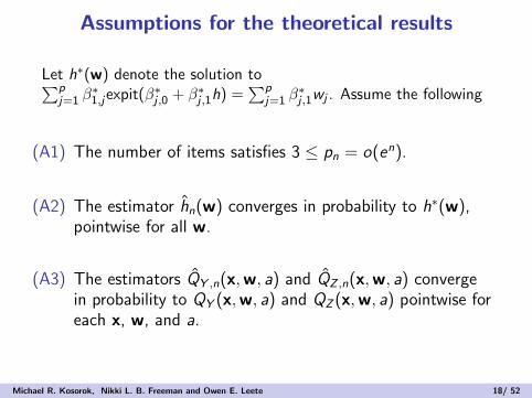
Assumptions for the theoretical results

Let h∗(w) denote the solution to∑pj=1 β

∗1,jexpit(β∗j ,0 + β∗j ,1h) =

∑pj=1 β

∗j ,1wj . Assume the following

(A1) The number of items satisfies 3 ≤ pn = o(en).

(A2) The estimator hn(w) converges in probability to h∗(w),pointwise for all w.

(A3) The estimators QY ,n(x,w, a) and QZ ,n(x,w, a) convergein probability to QY (x,w, a) and QZ (x,w, a) pointwise foreach x, w, and a.


Theoretical results

The first theoretical result establishes consistency of the proposedestimator for the optimal DTR as the sample size diverges but thenumber of items remains fixed.

Theorem (Thm 2.2 in Butler et al. (2018))

Assume (A1) - (A3) and let the number of items, pn = p, be fixed.Then VU(πopt)− VU(πn) converges to zero in probability asn→∞.

The second theoretical result says that if the number of items isallowed to diverge with the sample size then the estimated DTRperforms as well as an oracle that knows each patient’s individualpreference.

Theorem (Thm 2.3 in Butler et al. (2018))

Assume (A1) - (A3) and suppose pn →∞ as n→∞. ThenVU(πn)− VU(πoracle) converges to zero in probability as n→∞.


Case Study: CATIE

I The Clinical Antipsychotic Trials of InterventionEffectiveness (CATIE) schizophrenia trial was designed tocompare new antipsychotic drugs to conventional ones ina randomized, controlled, double-blind, multi-phase trial.

I The trial targeted patients already being treated forschizophrenia but who might benefit from a medicinalchange.

I Patients received antipsychotic treatments and wereoffered psychosocial treatment with their families.


First phase of CATIE

I The first phase of CATIE is suited for application of themethod proposed in Butler et al. (2018).

I Patients were randomized to one of 5 medications,I 4 were atypical antipsychotics, andI 1 was a conventional antipsychotic (perphenazine).

I For ease of exposition, we will dichotomize the treatmentsinto atypical antipsychotics and perphenazine.

I At baseline, patients answered a 10 question, binaryresponse assessment, which can be used to measurepatient preferences across two outcomes

I Efficacy using the Positive and Negative Syndromes Scale(PANSS), and

I Side effect burden measured as the sum of side effect andadverse event indicators.


Patient preference questionsThe patient preference information was collected using a 10question Drug Attitude Inventory assessment. One question wasexcluded from analysis.

Figure 1: Table 1 from Butler et al. (2018)


AnalysisTailoring covariates were selected based on clinical expertise andprior analyses.

Figure 2: Table 2 from Butler et al. (2018)


Analysis (cont.)

I By examining the coefficients for the Q-functions, we seethat the main effect of treatment has an opposite sign inthe two Q-functions as well as several interactionsinvolving treatment.

I This suggests a trade-off between the two outcomes thatmust be made in choosing a treatment and that this tradeoff varies across patient characteristics.


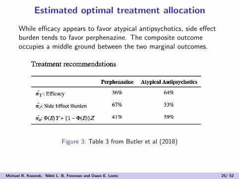
Estimated optimal treatment allocation

While efficacy appears to favor atypical antipsychotics, side effectburden tends to favor perphenazine. The composite outcomeoccupies a middle ground between the two marginal outcomes.

Figure 3: Table 3 from Butler et al (2018)


Percent agreement in treatment recommendations

This table shows the fraction of overlap between the proposedestimated optimal DTR and the optimal DTR based only onefficacy or side effect burden.

Figure 4: Table 4 in Butler et al. (2018)


Discussion

I Butler et al. (2018) propose a strategy for balancingmultiple, possibly competing outcomes when estimating adynamic treatment regime.

I A few other methods for incorporating multiple outcomesinto precision medicine have been proposed for variousscenerios under various assumptions. However, theliterature in this area is relatively small.

I An interesting extension is the multi-decision setting. Thisis a challenging extension as patient preferences maychange over time in response to treatment received andinterim outcome experiences.


Outline

Incorporating patient preferences

Estimation and Optimization of Composite Outcomes


Introduction

I Almost all methods for estimating individualized treatmentrules have been designed to optimize a scalar outcome

I Clinical decision making often requires balancingtrade-offs between multiple outcomes

I Examples:

I Bipolar disorder treatments must manage both depression andmania

I Antidepressants can prevent depressive episodes but may alsoinduce manic episodes

I Utility functions can be used to summarize multipleoutcomes as a single scalar


Setup and Notation

I We will assume two outcomes, but the method can beextended to more

I The available data are (Xi ,Ai ,Yi ,Zi), i = 1, . . . , n

I Xi ∈ X ⊆ Rp are patient covariates

I A ∈ A = {−1, 1} is a binary treatment

I Y and Z are two real-valued outcomes (higher is better)

I Let Y ∗(A) and Z ∗(A) be the potential outcomes undertreatment a

I We will need the standard causal assumptions

I Consistency: Y = Y ∗(A) and Z = Z∗(A)

I Positivity: Pr(A = a|X = x) ≥ c > 0

I Ignorability: {Y ∗(−1),Y ∗(1)} ⊥ A |X


Optimal Treatments for Individual Outcomes

I Define QY (x, a) = E(Y |X = x,A = a)

QZ (x, a) = E(Z |X = x,A = a)

I Under the preceding assumptions we have

I doptY (x) = argmaxa∈AQY (x, a)

I doptZ (x) = argmaxa∈AQZ (x, a)

I In general, doptY (x) need not equal dopt

Z (x)

I If both Y and Z are clinically relevant, neither doptY nor

doptZ may be acceptable


Utility Functions

I Define the composite outcome U = u(Y ,Z ) for a utilityfunction, u

I u : R2 7→ R is the “goodness” of the outcome pair (y , z)I u may be unknown and possibly depend on the covariates

I Define QU(x, a) = E(U |X = x,A = a)

I The optimal regime with respect to U satisfies

doptU (x) = argmax

a∈AQU(x, a)

= argmaxa∈A

E[u{Y (a),Z (a)} | x]

I Utility functions which are convex combinations ofQY (x, a) and QZ (x, a) are identifiable under the precedingassumptions


Inverse Reinforcement Learning

I We assume that clinicians act with the goal of optimizingeach patient’s utility

I Inverse reinforcement learning uses decisions made by anexpert to construct a utility function

I We assume that the clinicians are approximately (i.e.,imperfectly) assigning treatment according to dopt(x)

I There would be no need to estimate the optimal treatmentpolicy if the clinician were always able to correctly identify theoptimal treatment

I We assume that the probability of making the correcttreatment decision depends on individual patientcharacteristics

Pr{A = doptU (X) |X = x} = expit(xTβ)

where β is an unknown parameter


Fixed Utility

I We begin by assuming the utility function is constantacross patients

I Let the utility function be u(y , z ;ω) = ωy + (1− ω)z forsome ω ∈ [0, 1]

I The optimal ITR for a broad class of utility functions isequivalent to the optimal ITR for a utility function of thisform (Butler 2018, Lemma 1)

I Define Qω(x, a) = ωQY (x, a) + (1− ω)Qz(x, a) anddoptω (x) = argmaxa∈AQω(x, a)


Fixed Utility, Cont.

I Let QY ,n and QZ ,n be estimates based on regressionmodels fit to the observed data

I For a fixed value of ω, let

Qω,n(x, a) = ωQY ,n(x, a) + (1− ω)QZ ,n(x, a)

I Define dω,n(X) = argmaxa∈A Qω,n(x, a)

I The joint distribution of (X,A,Y ,Z ) is

f (X,A,Y ,Z ) = f (Y ,Z |X,A)f (A|X)f (X)

= f (Y ,Z |X,A)f (X)exp[XTβ1{A = dopt

ω (X)}]1 + exp(XTβ)


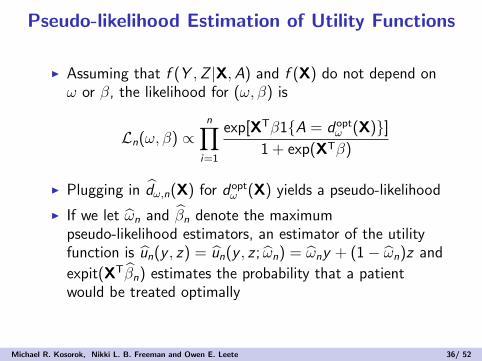
Pseudo-likelihood Estimation of Utility Functions

I Assuming that f (Y ,Z |X,A) and f (X) do not depend onω or β, the likelihood for (ω, β) is

Ln(ω, β) ∝n∏

i=1

exp[XTβ1{A = doptω (X)}]

1 + exp(XTβ)

I Plugging in dω,n(X) for doptω (X) yields a pseudo-likelihood

I If we let ωn and βn denote the maximumpseudo-likelihood estimators, an estimator of the utilityfunction is un(y , z) = un(y , z ; ωn) = ωny + (1− ωn)z and

expit(XTβn) estimates the probability that a patientwould be treated optimally


Algorithm

I The pseudo-likelihood is non-smooth in ω, so standardgradient-based optimization can’t be used

I For a given value of ω, it is straightforward to compute

the profile estimator βn(ω)

I Compute the profile pseudo-likelihood over a grid for ωand select the value yielding the largest pseudo-likelihood

I Finding βn(ω) can be accomplished using logisticregression


Patient-specific Utility

I In some application domains outcome preferences canvary widely across patients

I Schizophrenia

I Pain management

I etc.

I To accommodate this, we assume that the utility functiontakes the form u(y , z ; x, ω) = ω(x)y + 1− ω(x)z whereω : X 7→ [0, 1] is a smooth function

I e.g., Let ω(x ; θ) = expit(XTθ) where θ is an unknownparameter

I Define Qθ(x, a) = ω(x; θ)QY (x, a) + (1− ω(x; θ))QZ (x, a)and define dopt

θ (x) = argmaxa∈AQθ(x, a)


Patient-specific Utility

I For QY ,n, QZ ,n and a fixed value of θ, let

Qθ,n(x, a) = ω(x; θ)QY ,n(x, a) + (1− ω(x; θ))QZ ,n(x, a)

and doptθ,n (x) = argmaxa∈A Qθ,n(x, a)

I We can compute the estimators (θn, βn) by maximizingthe pseudo-likelihood

Ln(θ, β) ∝n∏

i=1

exp[XTβ1{A = dθ,n(X)}]1 + exp(XTβ)

I An estimator for the utility function is

un(y , z ; x) = ω(x; θn)y + (1− ω(x; θn))z

I An estimator for the optimal decision function is dθn,n


Algorithm

I As before, the pseudo-likelihood is non-smooth in θ

I It is again straightforward to compute the profile

pseudo-likelihood estimator βn(θ) for any θ ∈ Rp

I It is computationally infeasible to compute βn(θ) over agrid for moderate p

I Instead we generate a random walk through the parameterspace using the Metropolis algorithm (see next slide)

I After generating a chain (θ1, . . . , θB), we select the θk

that leads to the largest value of Ln(θk) as the maximumpseudo-likelihood estimator


Algorithm, Cont.

Algorithm 2: Pseudo-likelihood estimation of patient-dependentutility function

1 Set a chain length, B, fix σ2 > 0, and initialize θ1 to a startingvalue in Rp;

2 for b = 2, . . . ,B do3 Generate e ∼ N(0, σ2I );

4 Set θb+1 = θb + e;

5 Compute p = min{Ln(θb+1)/Ln(θb), 1};6 Generate U ∼ U(0, 1); if U ≤ p, set θb+1 = θb+1; otherwise,

set θb+1 = θb;

7 end


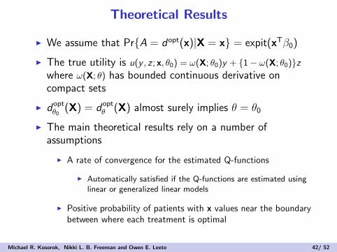
Theoretical Results

I We assume that Pr{A = dopt(x)|X = x} = expit(xTβ0)

I The true utility is u(y , z ; x, θ0) = ω(X; θ0)y + {1− ω(X; θ0)}zwhere ω(X; θ) has bounded continuous derivative oncompact sets

I doptθ0

(X) = doptθ (X) almost surely implies θ = θ0

I The main theoretical results rely on a number ofassumptions

I A rate of convergence for the estimated Q-functions

I Automatically satisfied if the Q-functions are estimated usinglinear or generalized linear models

I Positive probability of patients with x values near the boundarybetween where each treatment is optimal


Asymptotic Inference

TheoremUnder regularity conditions, the pseudo-likelihood maximizers βnand θn satisfy

√n

(θn − θ0βn − β0

)

(U

I−10 [ZA − k0(ZY ,ZZ ,U)]

)=

(UB

),

where U = argminu βT0 k0(ZY ,ZZ , u), and ZY

ZZ

ZA

∼ N(0,Σ0).

A certain semiparametric bootstrap is also consistent in probability.


Asymptotic InferenceMain technical tools:

I The Argmax theorem

I The following for the bootstrap:

Theorem

I Let H be compact with respect to a metric d andF ⊂ C [H] be compact with respect to ‖ · ‖H

I For each f ∈ F , let u(f ) = argmaxu∈H f (u), where wearbitrarily choose a value if nonunique

I Suppose also that there exists an F1 ⊂ F such that eachf ∈ F1 has a unique maximum

I Then

limδ↓0

supf ∈F1

supg∈F :‖f−g‖H<δ

d(u(f ), u(g)) = 0


Parametric Bootstrap

Theorem

I Assume Σn = Σ0 + oP(1)

I Let Z ∗ ∼ N(0, I r×r ) where r = p + q,

Zn = ΣnZ∗ = (ZT

Y , ZTZ , Z

TA )T

I Define Un = argminu∈Rd βTn kn(ZY , ZZ , u) and

Bn = In(βn)−1{ZA − kn(ZY , ZZ , Un)}I Then (

Un

Bn

)P Z∗

(UB

),

where U and B are as defined on slide 43


Simulation Studies

I X = (X1, ...,X5)T ∼ N(0,Σ = 0.52I )

I Y = A(4X1 = 2X2 + 2) + εYZ = A(2X1 − 4X2 − 2) + εZwhere εY ∼ εZ ∼ N(0, 0.52)

I Setting 1:I Pr{A = dopt(x) |X = x} = ρ

I Setting 2:I Pr{A = dopt(X)} = expit(0.5 + X1)

I Setting 3:I Pr{A = dopt(X)} = expit(0.5 + X1)I ω(X; θ) = expit(1− 0.5X1)


Simulation Results

I Value results for simulations where utility (ω) andprobability of optimal treatment (ρ) are fixed

n ω ρ Optimal Estimated ω Y only Z only Standard of care

100 0.25 0.60 1.90 (0.07) 1.75 (0.29) 0.39 (0.12) 1.77 (0.07) 0.39 (0.23)0.80 1.90 (0.07) 1.88 (0.07) 0.39 (0.12) 1.77 (0.07) 1.14 (0.21)

0.75 0.60 1.89 (0.07) 1.69 (0.40) 1.76 (0.08) 0.39 (0.12) 0.40 (0.23)0.80 1.89 (0.07) 1.89 (0.07) 1.76 (0.08) 0.39 (0.12) 1.15 (0.21)

200 0.25 0.60 1.90 (0.07) 1.80 (0.25) 0.39 (0.11) 1.77 (0.07) 0.38 (0.17)0.80 1.90 (0.07) 1.89 (0.06) 0.39 (0.11) 1.77 (0.07) 1.15 (0.15)

0.75 0.60 1.90 (0.07) 1.79 (0.26) 1.76 (0.07) 0.38 (0.11) 0.38 (0.17)0.80 1.90 (0.07) 1.89 (0.06) 1.76 (0.07) 0.38 (0.11) 1.16 (0.15)

300 0.25 0.60 1.90 (0.07) 1.86 (0.13) 0.37 (0.11) 1.76 (0.08) 0.38 (0.13)0.80 1.90 (0.07) 1.89 (0.07) 0.37 (0.11) 1.76 (0.08) 1.14 (0.12)

0.75 0.60 1.90 (0.06) 1.84 (0.19) 1.76 (0.08) 0.39 (0.11) 0.39 (0.13)0.80 1.90 (0.06) 1.90 (0.07) 1.76 (0.08) 0.39 (0.11) 1.15 (0.12)

500 0.25 0.60 1.90 (0.06) 1.88 (0.08) 0.38 (0.11) 1.77 (0.07) 0.37 (0.11)0.80 1.90 (0.06) 1.90 (0.06) 0.38 (0.11) 1.77 (0.07) 1.13 (0.09)

0.75 0.60 1.90 (0.07) 1.88 (0.08) 1.76 (0.08) 0.39 (0.11) 0.37 (0.10)0.80 1.90 (0.07) 1.90 (0.07) 1.76 (0.08) 0.39 (0.11) 1.13 (0.09)


Simulation Results

I Value results for simulations where utility (ω) is fixed andprobability of optimal treatment is variable

n ω Optimal Estimated ω Y only Z only SoC

100 0.25 1.90 (0.06) 1.72 (0.41) 0.40 (0.11) 1.76 (0.07) 0.33 (0.24)0.75 1.90 (0.06) 1.76 (0.29) 1.76 (0.07) 0.38 (0.12) 0.58 (0.24)

200 0.25 1.90 (0.06) 1.84 (0.24) 0.38 (0.11) 1.75 (0.08) 0.32 (0.16)0.75 1.90 (0.06) 1.84 (0.16) 1.76 (0.07) 0.38 (0.11) 0.57 (0.16)

300 0.25 1.89 (0.07) 1.88 (0.14) 0.38 (0.11) 1.77 (0.07) 0.32 (0.14)0.75 1.90 (0.07) 1.87 (0.09) 1.76 (0.07) 0.39 (0.12) 0.56 (0.14)

500 0.25 1.90 (0.07) 1.90 (0.06) 0.38 (0.11) 1.77 (0.07) 0.33 (0.10)0.75 1.90 (0.07) 1.89 (0.08) 1.76 (0.07) 0.39 (0.11) 0.57 (0.10)


Simulation Results

I Value results for simulations where both utility andprobability of optimal treatment are variable

n Optimal Estimated ω Y only Z only Standard of care

100 1.74 (0.06) 1.53 (0.19) 1.59 (0.07) 0.44 (0.11) 0.51 (0.21)200 1.73 (0.06) 1.61 (0.13) 1.59 (0.07) 0.44 (0.10) 0.51 (0.15)300 1.74 (0.06) 1.64 (0.12) 1.59 (0.07) 0.44 (0.10) 0.50 (0.13)500 1.74 (0.06) 1.68 (0.09) 1.59 (0.07) 0.43 (0.10) 0.50 (0.09)


Misspecified Model for the Utility Function

I Let the true underlying utility function beu(y , z ; bx , θ) = ωx; θ)y + {1− ω(x; θ)}z

I Where ω(x; θ) = expit(1 + x21 + xTθ0)I Consider a misspecified model fit to estimate the utility

function containing only an intercept, X1,X2,X3, and X4

I i.e., one important covariate and a squared term are omittedfrom the model for the utility function

n Optimal Correct Misspecified Standard of Care

100 1.86 (0.07) 1.61 (0.21) 1.64 (0.20) 0.59 (0.23)200 1.85 (0.07) 1.68 (0.16) 1.69 (0.17) 0.57 (0.16)300 1.86 (0.07) 1.72 (0.13) 1.74 (0.13) 0.57 (0.13)500 1.86 (0.07) 1.77 (0.10) 1.76 (0.11) 0.58 (0.10)


Analysis of STEP-BD SCP Data

I Included an observational study with 1437 patients havingbipolar disorder (Sachs et al, 2007, NEJM).

I Using the proposed method, we were able to estimate animproved decision rule which led to a 7% improvement(p-value < 0.0001).

I Both increased age and history of substance abuse wereimportant factors leading to lower recommended use ofantidepressants.

I If we selected the two outcomes to be depression and sideeffect burden, we obtain an improvement of 9% (p-value< 0.001).


Conclusions

I We can estimate patient utilities if we assume thatclinicians make treatment decisions with the goal ofmaximizing each patient’s utility

I Accounting for patient specific utilities can improveoutcomes over standard of care

I Early results suggest the method is robust to utility modelmisspecificaion, but more research is needed

I The approach could be extended to multiple decisiontimes, more than two outcomes, and more than twopossible treatments

I A Bayesian approach could be developed to handle thenon-smooth pseudo-likelihood


precision medicine: lecture 15 multiple utilities

Documents