precision agriculture for the sugarcane industry · implementing pa precision agriculture for the...
TRANSCRIPT

Precision Agriculture forthe Sugarcane Industry
TM

© Copyright 2015 by Sugar Research Australia Limited. All rights reserved. No part of the Precision Agriculture for the Sugarcane Industry (this publication), may be reproduced, stored in a retrieval system, or transmitted in any form or by any means, electronic, mechanical, photocopying, recording, or otherwise, without the prior permission of Sugar Research Australia Limited.
Disclaimer: In this disclaimer a reference to ‘SRA’, ‘we’, ‘us’ or ‘our’ means Sugar Research Australia Limited and our directors, officers, agents and employees. Although we do our very best to present information that is correct and accurate, we make no warranties, guarantees or representations about the suitability, reliability, currency or accuracy of the information we present in this publication, for any purposes. Subject to any terms implied by law and which cannot be excluded, we accept no responsibility for any loss, damage, cost or expense incurred by you as a result of the use of, or reliance on, any materials and information appearing in this publication. You, the user, accept sole responsibility and risk associated with the use and results of the information appearing in this publication, and you agree that we will not be liable for any loss or damage whatsoever (including through negligence) arising out of, or in connection with the use of this publication. We recommend that you contact our staff before acting on any information provided in this publication. Warning: Our tests, inspections and recommendations should not be relied on without further, independent inquiries. They may not be accurate, complete or applicable for your particular needs for many reasons, including (for example) SRA being unaware of other matters relevant to individual crops, the analysis of unrepresentative samples or the influence of environmental, managerial or other factors on production.
More information
We are committed to providing the Australian sugarcane industry with resources that will help to improve its productivity, profitability and sustainability.
A variety of information products, tools and events which complement this manual are available including:
• Information sheets and related articles
• Publications including soil guides, technical manuals and field guides
• Research papers
• Extension and research magazines
• E-newsletters and industry alerts
• Extension videos
• Online decision-making and identification tools
• Training events.
These resources are available on the SRA website and many items can be downloaded for mobile and tablet use. Hard copies for some items are available on request.
We recommend that you subscribe to receive new resources automatically. Simply visit our website and click on Subscribe to Updates.
www.sugarresearch.com.au
Acknowledgements
Some of the material covered in this publication is drawn from Precision and Smart Technologies in Agriculture: Study Book (Jensen 2013). This expertise and knowledge is gratefully acknowledged.
We thank the following contributors to this publication:
• Dr Rob Bramley, CSIRO Adelaide
• Phil Deguara, canegrower
• Bryan Granshaw, canegrower
• Dr Troy Jensen, University of Southern Queensland, National Centre for Engineering in Agriculture
• Liana Lillford and John McGillivray, Wilmar AgServices
• John Markley and Peter McDonnell, Farmacist Pty Ltd
• Kevin Moore, Mackay Area Productivity Services (MAPS)
• Andrew Robson, University of New England, Precision Agriculture Research Group
• Michael Sefton, Herbert Cane Productivity Services Ltd (HCPSL).
Contact details
Sugar Research Australia
PO Box 86
Indooroopilly QLD 4068 Australia
Phone: 07 3331 3333
Fax: 07 3871 0383
Email: [email protected]
ISBN: 978-0-949678-34-8

Table of contents01
02
02
03
04
05
06
07
08
09
09
09
10
10
10
10
11
12
13
13
15
15
16
17
19
19
20
20
20
20
21
21
22
23
24
24
25
25
26
27
28
29
30
31
32
32
33
33
34
35
36
36
37
37
38
38
40
42
43
44
46
Introduction
Background
Current status of PA in the Australian sugar industry
Implementing PA
PA technologies
More information
Global Positioning Systems (GPS) and other Global Navigation Satellite Systems (GNSS)
Types of GPS receivers
Factors that affect GPS accuracy
What to consider when buying a navigation system
Tractor satellite navigation
Benefits of satellite navigation
Economic benefits of controlled traffic
Controlled traffic in the Mackay district
Topographic mapping
Other agricultural uses of GPS
Glossary
Geographic Information Systems (GIS)
Components of a GIS
GIS and precision agriculture
AgDat: GIS for better farm management
Glossary
Remote Sensing (RS)
Electromagnetic spectrum
Agricultural uses of remote sensing
Methods of remote sensing
Normalised Difference Vegetation Index (NDVI)
Limitations of remote sensing
Use of RS in sugarcane
Obtaining remotely sensed images
Accurately forecasting yield with remotely sensed imagery
Glossary
Yield mapping
Yield monitors
Commercial yield monitors
Creating yield maps from yield monitor data
Creating yield maps from remotely sensed imagery
The future of yield mapping
Yield monitoring in the Herbert: a whole system approach
High-resolution soil mapping
Soil-apparent electrical conductivity (ECa)
Gamma radiometrics
Glossary
Variable-rate technology
Benefits of variable-rate application
Variable-rate equipment
Economics of VRT
Case study: Variable-rate Biodunder® now and into the future
Variable-rate irrigation (VRI)
Weed sensors
WeedSeeker® technology
WeedSeeker use in sugarcane
Limitations of commercial shields
Cost effectiveness
More information about WeedSeeker use in sugarcane
Economic viability of WeedSeeker technology in sugarcane
CCS sensors
Case studies
Bryan Granshaw: the new farming system
Phil Deguara: taking the long view
References

01
Introduction
Geographic Information Systems (GIS)
Weed sensors
PA technologies
Case studies ReferencesCCS sensors
Yield mapping High-resolution soil mapping
Remote Sensing (RS)
Variable-Rate Technology (VRT)
Global Positioning Systems (GPS) and other Global Navigation Satellite Systems (GNSS)

02
The uptake of PA in the Australian sugar industry has lagged behind many other Australian agricultural industries for several reasons. The growing and harvesting processes for sugarcane present some challenges not present in other industries with higher uptake of PA.
Also, sugarcane’s long growing season, coupled with a limited period for applying inputs, can make it difficult to implement the precise input rates required by PA, particularly for nutrients.
One of the biggest obstacles to PA has been the lack of a reliable commercial yield monitor and the ability to obtain accurate yield data under the current harvesting model.
Other factors affecting PA adoption include grower risk aversion, farm size versus technology cost, lack of cost-benefit data, and lifestyle preferences that may not coincide with PA management needs.
However, there are growers in the industry who have benefited from incorporating PA into well-thought-out farming systems. One area where the sugar industry has progressed significantly, largely due to government funding related to the Great Barrier Reef management, is in the uptake of GPS guidance for machinery.
In spite of the challenges, it is important for the sugar industry to continue working towards increased adoption of PA for the future robustness of the industry. As production costs increase, along with concern about the environmental impacts of agriculture, there is a need for increased efficiency on the farm and for growers to demonstrate that they are using the best available tools and practices. Also, growers need to continually develop their ability to be competitive in the modern marketplace.
Technologies that improve efficiency, save money and reduce environmental impacts will be adopted in greater numbers over time and are likely to become essential to the profitability of farming enterprises.
Soils and topography, two of the primary factors affecting agriculture, vary on both large and small scales. Farmers know this, and can often identify this variability from years of experience. Yet the majority of sugarcane farming is carried out in square or rectangular paddocks, which are often quite large, using uniform management practices.
Precision agriculture (PA) is a farm management technique that addresses the variability of the land and resulting variability in yield to improve farm productivity and profitability. PA can also help address variability in weed, pest and disease occurrence and moisture supply. Although the term is relatively new, PA has been around for hundreds of years. In its current form, PA is often associated with technologies such as GPS, GIS and variable-rate applicators. The use of technology does not always automatically lead to PA but, in sugarcane production, technology is used for most PA practices, and that is the focus we will take in this guide.
Research and application of PA in the Australian sugar industry began in the 1990s, but a collapse in world sugar prices, low yields and ongoing issues with sugarcane yield monitors essentially halted the progress of PA in the industry in the late 90s. A few individual growers continued to pursue PA solutions for their own farms, and several factors led to a renewed interest in industry-wide potential for PA several years ago.
In 2007, the Sugar Research and Development Corporation funded a technical report, Precision agriculture options for the Australian sugarcane industry (SRDC Technical Report 3/2007). This report determined that PA was an area of opportunity for the industry and identified research and development needs as well as the status of current technologies as they relate to sugar production. SRDC subsequently funded a large PA research and development project with smaller projects emerging in the ensuing years. This research push, along with government assistance to growers for the purchase of PA-related technologies, has created a renewed interest in PA. Current research is providing the information necessary to further PA adoption in this industry.
Background
Current status of PA in the Australian sugar industry
Introduction

Implementing PA
Precision Agriculture for the Sugarcane Industry
03
We have already defined PA as identifying and managing variability on the farm and in productivity. In cropping industries, this is also termed site-specific crop management (SSCM). PA or SSCM can be considered as the application of information technologies, together with production experience, to:
• optimise production efficiency
• optimise crop quality
• minimise environmental impacts
• minimise risk to the grower.
PA is not simply the use of GPS or other technologies, though there are many technologies that can be incorporated into a PA management strategy. PA is a process that should be part of an overarching farm management plan, with clear goals the grower wants to achieve.
Figure 1 illustrates the cyclical process of PA. To increase the likelihood of achieving desired outcomes, growers should follow this process without skipping steps. Following established procedures also helps growers to determine whether or not outcomes are a result of PA management or other factors.
1. Recognise the potential opportunity to better manage field or farm variability.
2. Collect spatial information, such as yield maps and high-resolution soil maps.
3. Put all of this information together (usually in a GIS program) and analyse it.
4. Create a management plan that addresses variability in soils, yield potential, or other factors identified as important.
5. Evaluate the targeted management plan to determine whether it has had the desired improvements, to continue to collect yield and other information over time, and to adjust farm management as necessary. Because the PA process is a cycle, it is important to complete this step.
In this publication we will discuss many of the PA technologies that are currently available and how they can be applied in the sugar industry. We will also look at examples from throughout the industry of growers and organisations that have succeeded with PA practices. Finally, we will look at some growers who have incorporated multiple PA tools into their farm management strategy over time.
Figure 1: The precision agriculture process (Bramley 2011).
1. Observation
3. Targeted management plan
2. Evaluation and interpretation
The primary source of information is a yield map (left) or sometimes, a remotely sensed image.
E.g. targeted application of fertilizer, irrigation water, agrochemicals, soil ameliorants or crop ripeners, selective harvesting, etc.
Supplementary sources of information are invaluable. These may include: remotely sensed imagery, a digital elevation model, high resolution soil mapping (e.g. EMI (above), gamma radiometry, GPR), soil and tissue testing and crop assessment.
The process of precision agriculture
Low Med High
Low Med High
04
PA technologies
Geographic Information Systems (GIS)
Weed sensors Case studies ReferencesCCS sensors
Yield mapping High-resolution soil mapping
Remote Sensing (RS)
Introduction
Variable-Rate Technology (VRT)
Global Positioning Systems (GPS) and other Global Navigation Satellite Systems (GNSS)

PA technologies
05
PA technologies are those used to complete the process outlined in Figure 1 on Page 3 (The Process of Precision Agriculture). Many of the key PA technologies were developed in industries not traditionally associated with agriculture. They might challenge some ideas of what it means to be a grower. Those who take the time to learn more about these technologies and their applications in sugarcane production will see that PA can result in significant benefits in productivity and profitability.
This guide is not intended to be a thorough technical guide to each of the technologies discussed. More detailed technical information is available elsewhere, including in the reference list.
The following links are good starting points for more in-depth information:
• Grains Research and Development Corporation
Applying PA – A reference guide for the modern practitioner
www.grdc.com.au/ApplyingPA
• Jensen T. 2013. Precision and Smart Technologies in Agriculture: Study Book. University of Southern Queensland, Faculty of Engineering and Surveying. 166 pp.
• Precision Cropping Technologies Pty Ltd
www.pct-ag.com
• Precision Ag Help Desk
www.pahelpdesk.com
• University of Sydney
Precision Agricultural Laboratory, Educational Resources
www.sydney.edu.au/agriculture/pal/publications_references/educational_resources.shtml
There are several resources on this page. The Precision Agriculture: Education and Training Modules for the Australian Grains Industry provide both basic and advanced information about PA technologies that are used in a variety of agricultural industries.
More information
• SPAA Precision Agriculture Australia
A non-profit organisation that promotes the development and adoption of precision agriculture (PA) technologies in Australia
www.spaa.com.au/communications.php
• Sugar Research Australia
Growing cane – Precision agriculture
www.sugarresearch.com.au/page/Growing_cane/Precision_agriculture/
Precision Agriculture for the Sugarcane Industry

06
Global Positioning Systems (GPS) and other Global Navigation Satellite Systems (GNSS)
Geographic Information Systems (GIS)
Weed sensors Case studies ReferencesCCS sensors
Yield mapping High-resolution soil mapping
Remote Sensing (RS)
Introduction
Variable-Rate Technology (VRT)
PA technologies

Global Positioning Systems (GPS) and other Global Navigation Satellite Systems (GNSS)
07
Satellite-based navigation systems are the enabling technology of precision agriculture. They provide a relatively simple and robust technique for identifying any location on the Earth’s surface. This technique allows agricultural and environmental activities to be linked to the locations where they take place and analysed in relation to other activities. A variety of satellite-based navigation tools are available to suit different agricultural needs.
Global Navigation Satellite Systems (GNSS) is the standard industry term for satellite-based navigation systems. GPS, short for Global Positioning Systems, is the term more generally used to describe this technology. However, GPS is specific to the US Department of Defense NAVSTAR positioning system. Other systems are being developed by different countries, though the only other system with complete worldwide coverage is Russia’s GLONASS.
In GNSS, satellites orbit the earth and send signals to receivers that can give highly accurate information about their location on the Earth’s surface. Availability of multiple satellite systems can help improve the availability of signals, but only if the equipment is able to receive signals from each system.
Different levels of positioning accuracy are available, depending on what the receiver will be used for. Not surprisingly, higher accuracy comes at a higher price. Table 1 gives an overview of the main GPS options currently available, their accuracy, cost, and potential agricultural uses.
Precision Agriculture for the Sugarcane Industry
Types of GPS receivers
Table 1: Types of GPS receivers and their uses.
Type of GPS Accuracy Average cost Agricultural uses
Stand-alone receiver
Usually a handheld unit that receives satellite signals.
~ 4–10 m AU $100–1000 • Recording location of on-farm activities such as soil and tissue tests
• Strategic trials
Differential receiver (DGPS)
Receiver with a fixed, ground-based reference station to correct errors in original signal. May require a subscription.
~ 0.1–1 m Up to AU $10,000 • Recording location of on-farm activities such as soil and tissue tests
• Strategic trials
• Guidance
• Yield mapping
• Variable-rate control
Real-Time Kinematic (RTK) differential receiver
Type of differential receiver; correction signal comes from a local base station in real time. Generally, single, fixed, local base stations are limited to ranges less than 30 km.
2–10 cm AU $10,000–
40,000
• Recording location of on-farm activities such as soil and tissue tests
• Strategic trials
• Guidance
• Yield mapping
• Variable-rate control
• Auto steer
• Elevation mapping
• Land levelling and forming

The most common type of GPS used in precision agriculture is RTK. The accuracy of different RTK systems varies slightly. Users should understand the terminology dealers are using before deciding what to buy.
08
Figure 1: Handheld stand-alone GPS receiver.
Figure 3: A differential GPS system uses a ground-based reference station to give more-accurate location information. RTK receivers get their correction signal from a local base station in real time (www2.ca.uky.edu/agc/pubs/pa/pa5/pa5.htm).
Many factors can affect GPS accuracy. GPS users cannot control most of them, but understanding them can make GPS use more effective. Some factors to consider when operating a GPS receiver on the farm include the following:
• Number of satellites in view
Four satellites are needed to obtain a signal. Objects such as buildings, trees and hills can interfere with satellite signals and reduce the number of available signals.
• Satellite geometry
Because GPS satellites are constantly moving, their position relative to a given point will vary throughout the day. Satellites that are closely spaced will reduce accuracy.
• Clock errors
The quality of clocks in GPS receivers is poor compared to atomic clocks in satellites.
• Inconsistencies in the Earth’s atmosphere
• Multipath errors
When GPS signals reflect off hard objects such as buildings, the distance travelled to the receiver is further than if it had travelled to the receiver directly. This can cause small errors, usually 1 to 2 metres.
Figure 2: Example of a differential GPS receiver used for satellite navigation. The top image shows the GPS receiver and the antennae that receives the differential signal mounted on top of the tractor. The bottom image shows the tractor operator using the in-cab display for GPS guidance in the field.
Factors that affect GPS accuracy

Equipment needed for satellite navigation will vary, depending on the type of navigation and the machinery it is installed on. Local resellers can give information about the available options, and other growers can offer valuable insight about what has worked for them.
Growers should consider the following points when thinking of buying a vehicle navigation system:
• compatibility of systems with existing machinery
• transferability between machines
• ability for equipment to be upgraded
• software requirements
• availability of after-sales support services
• ongoing costs, particularly DGPS subscription fees
• ease of use
• diversity of swathing options
• signal tracking quality
• local base station networks.
The most common use of GPS in agriculture is for navigation. Below are three terms that explain different navigational uses of GPS. Sometimes these terms are used interchangeably, but they actually mean different things.
• Guidance
GPS guides machinery but the operator controls it. The guidance system uses a signalling device to prompt the driver to maintain a predetermined path. It needs sub-metre accuracy of GPS signal.
• Auto steer
Removes operator from most steering operations. For safety, auto steer systems have an automatic override system as soon as the operator takes control of the steering wheel. These systems also monitor the quality of the satellite signal. It needs centimetre accuracy of GPS signal.
• Controlled traffic
The use of guidance or auto steer to confine all machinery loads to permanent traffic lanes.
Satellite navigation can make farming operations more efficient and help growers to save time and money. Some of the benefits include:
• less skip and overlap of inputs
• less driver fatigue
• less compaction
• better soil water management
• higher yield
• more accurate inter-row cultivation, spraying and planting.
Precision Agriculture for the Sugarcane Industry
09
What to consider when buying a navigation system
Tractor satellite navigation
Benefits of satellite navigation
Figure 4: Illustration of the amount of ground compacted during harvesting on a farm with traditional 1.5 m row spacing (top) compared with a controlled-traffic system (bottom). In the traditional system, tyre tracks do not match row spacing, which increases the area of compacted ground.
Figure 5: Dual-row, controlled-traffic farming system in which tyre tracks are confined to relatively narrow traffic lanes between beds.
1.5 m row spacing
1.83 m harvester/haulout track width
Dual rows (500 mm) at 1.8 m row spacing
1.83 m harvester/haulout track width

• tractor power requirements reduced by at least 30 per cent
• faster access to field after rain
• greater infiltration of rainfall, resulting in less run-off
• better soil health, with more plant-available water
• less tillage after harvests.
High-accuracy positioning receivers used for giving locations in a paddock also measure elevation. Elevation information is regarded as being 1.5 to 2 times less accurate than the stated accuracy of the GPS receiver used. For example, a quoted receiver accuracy of 2 cm would translate into a 3 to 4 cm accuracy of elevation data.
Elevation data can be mapped onto a grid to form a digital elevation model (DEM) of the paddock or farm. The DEM is useful because it provides information on the potential movement and ponding of water within a paddock, on areas at risk from frost, and on locations where soil type may change. The DEM can also be used to calculate other topographical properties, such as aspect, slope, water shedding, and accumulation points. These, in turn, can indicate differences in clay content, soil depth or nutrient status. The DEM is also often used as a data layer in the process of selecting soil-sampling sites. Growers who use auto steer on their tractor or spray rig can log the elevation data. They should ask their provider to show them how to turn the elevation logging capability on.
As listed in the table on Page 7, there are a variety of agricultural uses of GPS besides navigation. A common thread in all of these activities is the use of spatial data. Access to specific information about where different things are happening on the farm can help growers better understand their land and give them more confidence in making management decisions.
Besides spatial information provided by GPS, agricultural GPS equipment and accompanying software can be used for things like automated record keeping and inter-vehicle communications. Understanding their equipment and all of its capabilities can help growers streamline farming operations to become more efficient and productive.
An analysis of 2013 productivity data from the Mackay district illustrates the benefits of controlled-traffic farming (CTF) over conventional farming. Of nearly 60,000 ha of sugarcane in the district that year, approximately 16,600 ha (28 per cent) was CTF (with or without GPS on all equipment). These farms use 1.8–2 m row spacing because the row widths are most suited to harvesting and haulout equipment.
Figure 6: 1.8 vs. 1.5 m row spacing.
Yield data from the mill show no significant differences in yield between the CTF row spacing and row widths that are less than 1.8 m. The graph above shows similar yields for 1.8 m and 1.5 m row spacings for various crop ages. The advantage of the wider rows is that there are fewer total rows in a block and, as a result, fewer passes are needed for farming activities.
This analysis concluded that the move from 1.5 m rows to 1.8 m rows reduced the required travel per hectare by 1100 m, and reduced overall growing costs by $153/ha. The important thing to remember with CTF is not that rows have to be a certain width, but that they must match the machinery wheel widths. Most growers who have adopted controlled traffic also use zonal tillage and fallow legumes to further reduce costs and improve the overall farming system.
10
Economic benefits of controlled traffic Topographic mapping
Other agricultural uses of GPS
Controlled traffic in the Mackay district
Yiel
d t/
ha
Crop age in years
100
90
80
70
60
50
40
30
20
10
0
0 2 4 6 8
1.8 m row spacing
1.5 m row spacing

Auto steer
A form of GPS guidance that removes the vehicle operator from most steering operations. For safety, auto steer systems have an automatic override system as soon as the operator takes control of the steering wheel. These systems also monitor the quality of the satellite signal. Auto steer needs a GPS signal with centimetre accuracy.
Controlled-traffic farming
The use of guidance or auto steer to confine all machinery loads to the least possible area of permanent traffic lanes.
Differential satellite navigation (commonly known as DGPS)
Enhanced GPS that provides better location accuracy using a network of fixed, ground-based reference stations to broadcast the difference between the positions indicated by the satellite systems and the known fixed positions. Corrections can be via radio and the AMSA beacon network, or by a satellite-delivered subscription service (e.g. OmniStar).
GLONASS
Russian GNSS, an alternative to the US NAVSTAR GPS, is the only other navigational system in operation with global coverage and of comparable precision.
GNSS (Global Navigation Satellite System)
A system of satellites (incorporating the US and Russian constellations) that provide autonomous geospatial positioning with global coverage. A GNSS allows small electronic receivers to determine their location (longitude, latitude and altitude) to high precision (within a few metres) using time signals transmitted along a line of sight by radio from satellites.
GPS (Global Positioning System)
GNSS maintained by the US Department of Defense that provides location and time information in all weather conditions, anywhere on or near the Earth where there is an unobstructed line of sight to four or more GPS satellites. The term GPS is often used more generically to refer to any GNSS.
Guidance
GPS guides machinery while the operator controls the vehicle. The guidance system uses a signalling device to prompt the driver to maintain a predetermined path. Guidance needs GPS signal with sub-metre accuracy.
RTK (Real Time Kinematic) satellite navigation
A form of differential satellite navigation (or DGPS) that relies on a local base station to provide real-time corrections, providing up to centimetre-level accuracy. With reference to GPS, this system is also referred to as Carrier-Phase Enhancement, or CPGPS.
Precision Agriculture for the Sugarcane Industry
11
Glossary

12
Geographic Information Systems (GIS)
Weed sensors Case studies ReferencesCCS sensors
Yield mapping High-resolution soil mapping
Remote Sensing (RS)
Introduction
Variable-Rate Technology (VRT)
PA technologies Global Positioning Systems (GPS) and other Global Navigation Satellite Systems (GNSS)

Geographic Information Systems (GIS)
13
Geographic Information Systems (GIS) are software packages that allow users to:
• create and overlay numerous maps
• manage data associated with maps
• analyse and manipulate data from multiple map layers.
Using a GIS is not as easy as many other types of software such as Microsoft Word or Google Earth. The five basic elements to consider in the use of a GIS are:
• data
• user
• software
• hardware
• methods.
Data
Data in a GIS context refers to any set of records that includes spatial information; that is, information linked to a specific location or ‘space’ on the Earth’s surface. Some examples are yield maps, soil maps, elevation maps, rainfall and weather data. Information might be linked to a region, town, farm or field or even to latitude and longitude coordinates. A GIS can analyse data in ways that other software can’t. But remember, good quality outcomes require good quality data.
User
User refers to the operator of a GIS. The operator must be able to ‘tell’ the GIS what they want for it to be effective. The operator also needs to be able to relate information from the GIS back to what is actually happening on the ground.
Software
Software is a computer package used to analyse the data. Many different types of GIS software are available, with the most common being ArcGIS and MapInfo. Many farm management
Components of a GIS
software packages also offer GIS components, including PAM, SMS, Farm Works, AgInfo GIS, SSToolbox, JD Office/Apex and more. Because costs and options vary greatly, growers and others interested in buying GIS software should do some research and find out which software will best meet their needs, and whether it is compatible with their other software and equipment.
Hardware
Hardware refers to the computer running the software. Generally, running a GIS requires a fast computer with a large storage capacity, primarily due to the many calculations required for analyses. A large monitor is also helpful for easy viewing of multiple menus, tables and images.
Methods
Methods are the techniques, models, classifications and mathematical reasons that guide GIS use and analysis, and display of information.
Because most precision agriculture data are spatial, they are related to a specific location. Using a GIS is the most effective way to manage spatial information and perform analyses that can help growers make decisions.
Some examples of data layers growers might use include:
• soil type
• elevation (topography)
• crop yield
• crop quality
• field boundaries
• management zones
• remotely sensed imagery
• weed and pest locations
• historical land use.
Precision Agriculture for the Sugarcane Industry
GIS and precision agriculture

Farmers often know from experience where high- and low-yielding areas on their farm are, or where they have particular problems. The value of using GIS to record and analyse this information is that growers can keep records over time and compare multiple data sets (for example, soils, yield and elevation) at the same time to create management zones.
When this information is in digital form, variable-rate prescriptions can be created and directly transferred into a tractor display unit with GPS capability to streamline a site-specific management system.
14
It is important to remember that the information generated by GIS depends on the quality of information put into the program. For the most reliable results, only high-quality data layers should be used for analysis.
Farmers who can’t afford GIS software or who are not interested in spending the time to analyse data layers should consider hiring a consultant to help with these tasks. Some productivity service groups offer GIS information and support, or they may be able to advise growers on project funding available for these types of services.
Figure 1: Researchers overlaid high-resolution soils maps (bottom layer), yield information from remotely sensed imagery (middle layers), and elevation data collected via GPS in ArcGIS to create management zones (top layer) for this paddock. Growers can develop their own management zones by buying farm management software with a GIS component, or working with a consultant who has experience with GIS.
CSE022 – Burdekin field site – Paddock zoning 2010-2011
EM38 soil surveyIkonos satellite imageryElevation via RTK GPS
Vertical exaggeration x 30
Elevation range = 2.57 m
Rob Bramley, CSIRO, Waite Campus, Adelaide
Zones
2011
2010
EM38
117a
85b
0.58
0.62
0.45
0.53
mS/m 2010 2011
Low
Med
High
NDVI
< 70
70–80
80–90
90–100
100–110
110–120
> 120
ECa (mS/m)
Precision Agriculture for the Sugarcane Industry
15
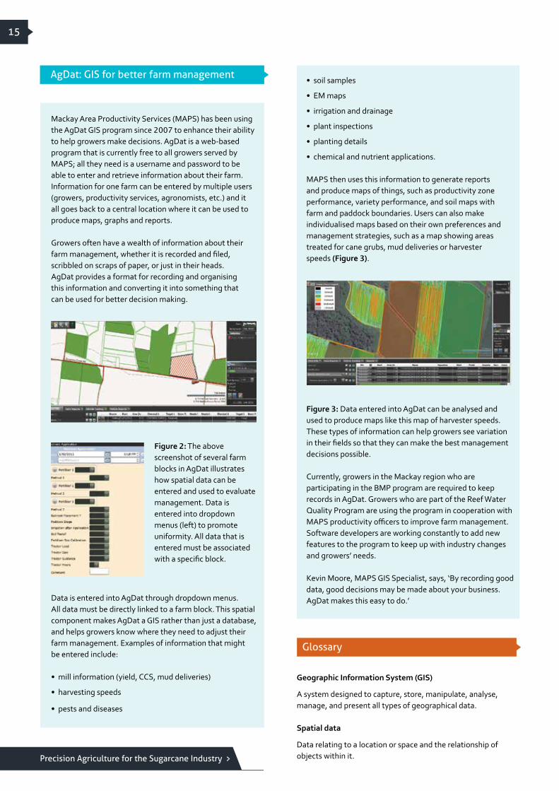
Mackay Area Productivity Services (MAPS) has been using the AgDat GIS program since 2007 to enhance their ability to help growers make decisions. AgDat is a web-based program that is currently free to all growers served by MAPS; all they need is a username and password to be able to enter and retrieve information about their farm. Information for one farm can be entered by multiple users (growers, productivity services, agronomists, etc.) and it all goes back to a central location where it can be used to produce maps, graphs and reports.
Growers often have a wealth of information about their farm management, whether it is recorded and filed, scribbled on scraps of paper, or just in their heads. AgDat provides a format for recording and organising this information and converting it into something that can be used for better decision making.
Data is entered into AgDat through dropdown menus. All data must be directly linked to a farm block. This spatial component makes AgDat a GIS rather than just a database, and helps growers know where they need to adjust their farm management. Examples of information that might be entered include:
• mill information (yield, CCS, mud deliveries)
• harvesting speeds
• pests and diseases
AgDat: GIS for better farm management• soil samples
• EM maps
• irrigation and drainage
• plant inspections
• planting details
• chemical and nutrient applications.
MAPS then uses this information to generate reports and produce maps of things, such as productivity zone performance, variety performance, and soil maps with farm and paddock boundaries. Users can also make individualised maps based on their own preferences and management strategies, such as a map showing areas treated for cane grubs, mud deliveries or harvester speeds (Figure 3).
Figure 3: Data entered into AgDat can be analysed and used to produce maps like this map of harvester speeds. These types of information can help growers see variation in their fields so that they can make the best management decisions possible.
Currently, growers in the Mackay region who are participating in the BMP program are required to keep records in AgDat. Growers who are part of the Reef Water Quality Program are using the program in cooperation with MAPS productivity officers to improve farm management. Software developers are working constantly to add new features to the program to keep up with industry changes and growers’ needs.
Kevin Moore, MAPS GIS Specialist, says, ‘By recording good data, good decisions may be made about your business. AgDat makes this easy to do.’
Geographic Information System (GIS)
A system designed to capture, store, manipulate, analyse, manage, and present all types of geographical data.
Spatial data
Data relating to a location or space and the relationship of objects within it.
Glossary
Figure 2: The above screenshot of several farm blocks in AgDat illustrates how spatial data can be entered and used to evaluate management. Data is entered into dropdown menus (left) to promote uniformity. All data that is entered must be associated with a specific block.

16
Remote Sensing (RS)
Weed sensors Case studies ReferencesCCS sensors
Yield mapping High-resolution soil mapping
Introduction
Variable-Rate Technology (VRT)
PA technologies Global Positioning Systems (GPS) and other Global Navigation Satellite Systems (GNSS)
Geographic Information Systems (GIS)

Remote Sensing (RS)
17
Remote sensing (RS) is the acquisition of information about an object without making physical contact with the object. This method can be especially useful in a crop like sugarcane, because physical access to it is difficult once it reaches a certain size.
Remote sensing imagery is as an integral part of a precision agriculture system as it provides another way to identify crop variability, via the spectral reflectance characteristics of the canopy. Growers can use this information to identify under-performing parts of paddocks, thus guiding targeted agronomy to identify the nature of the biotic or abiotic constraint.
In agriculture, remote sensing generally refers to imagery obtained from satellites, aircraft (including unmanned aerial vehicles (UAVs)) or proximal sensors. Generally, growers are most interested in variability in soil and crops, but RS imagery can be used for a variety of other purposes as well. There are many different sources of remotely sensed imagery with varying resolutions (levels of detail, pixel size on the ground) and scene sizes (area covered by an image).
Figure 1: High-resolution (left, IKONOS 0.8 m resolution) and low-resolution (right, SPOT 10 m resolution) satellite imagery of macadamia trees and sugarcane. Note the much higher level of detail of the high-resolution imagery. However, low-resolution imagery can still be useful for certain tasks and is often cheaper. Images courtesy of Andrew Robson, UNE-PARG.
Electromagnetic spectrum
In the electromagnetic spectrum there are many different types of waves with varying frequencies and wavelengths. Electromagnetic waves always travel at the speed of light, and their length depends on the source. For example, power lines are low-frequency, meaning the wavelength is long; gamma rays are high-frequency, meaning the wavelength is short (Figure 3).
The human eye can detect wavelengths from about 400 nm (violet) to about 700 nm (red). Remote sensing can be used to obtain imagery of multiple frequencies and wavelengths, including those that are not visible to human eyes. Imagery that measures several light wavelengths at the same time is called multispectral imagery.
Remotely sensed imagery is collected in digital format and can be stored in layers representing the different wavelengths or bands of light. Common layers include red, green, blue and near-infrared (NIR), which human eyes cannot see. With the information stored in layers, different combinations can be used to focus on different physical aspects of crop growth.
All matter reflects, absorbs and transmits electromagnetic energy in a unique way. Vegetation has a unique combination of emitted, reflected or absorbed energy called a spectral signature, which enables it to be readily distinguished from other types of land cover in NIR imagery. Additionally, in the non-visible range, reflectance among plant species is highly variable so multispectral imagery can provide a wealth of information on objects that may appear similar in the visible portion of the spectrum.
Precision Agriculture for the Sugarcane Industry
Macadamia trees
Sugarcane
Figure 2: High-resolution image of a sugarcane field, showing a canegrub incursion.

18
Figure 3: Diagram of the wavelength and frequency ranges of electromagnetic radiation. The visible portion of the electromagnetic spectrum is the narrow region with wavelengths between about 400 and 700 nm. Image source from 2012books.lardbucket.org/books/principles-of-general-chemistry-v1.0/s10-01-waves-and-electromagnetic-radi.html
The spectral characteristics of plants can be measured with either passive sensors, i.e. those that measure the reflectance/absorbance of solar radiation, or with active sensors that emit their own light source. A major benefit of active sensors is their ability to work under cloudy conditions and even at night. Two common active sensors include the Trimble GreenSeeker (www.trimble.com/agriculture/gs-handheld.aspx) and the Holland Scientific Crop Circle (www.hollandscientific.com) (Figure 4).
The GreenSeeker incorporates a series of three photo-detectors (PD) which measure visible red and a near infrared spectral information. These two bands are ratio-ed through a Normalised Difference Vegetation Index (NDVI) to provide an output indicating crop greenness or vigour. The Crop Circle contains three polychromatic (white) LEDs, which illuminate a target area, as well as three circular sensors in the centre of the device (labelled 1,2,3 Detector Channel). The spectral sensitivity of the sensors can be customised, with individual narrow band filters allowing measurements of relative target radiance in specific wavebands.
Figure 4: Active sensors: Holland Scientific Crop Circle; handheld GreenSeeker; and airborne Raptor Sensor (University of New England).
Passive sensors include satellite, airborne and unmanned aerial vehicles (UAV) platforms (Figure 5), as well as field-based hyperspectral radiometers.
Figure 5: Examples of satellite platform (QuickBird) and UAV (Octocopter).
Satellites currently available offer a wide array of spectral and spatial resolutions. The spectral resolution refers to the number of band widths provided, i.e. multispectral or hyperspectral and the spectral regions they encompass.
In the last decade, the use of commercial remote sensing platforms has increased rapidly, greatly improving the resolution of the data, the repeat time and commercial affordability. Subsequently, the degree of research, development and adoption has also increased.
Wavelength (nm)
Wavelength (nm)
10-12 10-11 10-10 10-9 10-8 10-7 10-6 10-5 10-4 10-3 10-2 10-1 100 101
1020 1019 1018 1017 1016 1015 1014 1013 1012 1011 1010 109 108
Frequency (Hz)
400 450 500 550 600 650 700
Visible spectrumV
iole
t
Blu
e
Gre
en
Yello
w
Ora
nge
Red
Gamma Ultraviolet Infrared Microwave RadioX-ray

Satellite Minimum swath Cost per km2 Cost per image Spatial resolution Revist time
SPOT–2 3600 km2 $0.69 AU $2500 20 m 1–4 days
SPOT–5 3600 km2 $0.96 AU $3465 10 m 1–4 days
SPOT–2 3600 km2 $2.67 AU $9600 2.5 m (pan*) 1–4 days
RapidEye 5000 km2 $2.70 US $13500 5 m 2 per day
QuickBird 78 km2 $28.20 US $2200 0.6 m (pan*) 1–3.5 days
IKONOS 100 km2 $34.20 US $3420 0.8 m (pan*) 1–3 days
IKONOS 50 km2 x 3 $22 US $3300 0.8 m (pan*) 1–3 days
Remote sensing is a management tool that captures colour, shape or other characteristics to identify spatial variability. A series of images collected over time can show changes in plant growth, soils, erosion or other physical processes. Some agricultural uses of remote sensing include:
• estimating crop yields
• detecting diseases
• identifying pest and weed coverage
• evaluating uniformity of irrigation
• observing changes in plant growth over time
• assessing the impact of severe weather
• determining the location and extent of crop stress.
Since sugarcane is a crop that cannot be easily observed once it reaches a certain height, RS can be a useful management tool that doesn’t require physical access to the crop. Problems within a field may be identified remotely before they can be identified on the ground.
Satellite
Table 1 lists some common RS satellites and information about the types of imagery they collect. Because satellites are constantly orbiting the Earth, imagery for a particular area is available only when the satellite passes overhead, regardless of the weather. This can be troublesome in some sugarcane-growing areas where images are often obscured by clouds, especially during the growing season.
Table 1: A selection of commercially available, remotely sensed satellite imagery.
Precision Agriculture for the Sugarcane Industry
19
Agricultural uses of remote sensing
Methods of remote sensing
Figure 6: QuickBird satellite imagery of a farm in colour (top) and multispectral, including colour and NIR (bottom). Images courtesy of Troy Jensen, USQ-NCEA.
*Pan is short for panchromatic, which means sensitive to all visible light.

20
Aerial imagery
Aerial imagery has the advantages of flexible flight times and high resolutions. It may also be more affordable for those who require imagery of a relatively small area. Generally, aerial imagery can be acquired and processed rapidly for good turnaround times, and atmospheric conditions have less of an effect than they do on satellite imagery. However, the scene size depends on the elevation of the aircraft, and higher resolution generally results in a smaller scene size. Because aircraft are less stable than satellites, imagery can have distortion problems. Also, it can be difficult to merge multiple scenes from aerial imagery.
A basic calculation that is often used to determine crop vigour is a ratio of NIR and red bands of light, sometimes called the vegetation index (VI). Vegetated surfaces will provide a high value for the ratio. The most commonly used ratio is the Normalised Difference Vegetation Index (NDVI), which provides information on plant greenness, vigour or health. It is sensitive to low chlorophyll concentrations, the amount of vegetation cover and solar radiation.
The NDVI is normally calculated across the crop’s vegetative growth period, and can be related to things such as biomass, leaf area index, percentage groundcover, nutrition, disease/damage and final yield.
Remotely sensed imagery can highlight variability at a paddock, farm or regional scale. However, even with proper calibration, it can be difficult to determine consistent direct relationships between measured reflectance and actual plant characteristics. Many factors complicate this relationship, such as atmospheric effects, differences between crop varieties, and climatic variation.
For these reasons, satellite data are not, in general, suitable on their own for determining absolute values of biomass or yield. However, they can be very useful in calculating relative values. To gain the most from remotely sensed data, field validation is essential. Images or maps should be used with direct sampling of the crop or soil to measure the attribute of interest. Sampling points are generally located across the range of variability to determine whether a relationship between the imagery and the attribute can be established.
Remote sensing has been used for many different purposes in sugarcane growing and harvesting. Some potential uses of imagery may include:
Normalised Difference Vegetation Index (NDVI)
Limitations of remote sensing
Use of RS in sugarcane
• forecasting regional yield
• producing farm-level and block-level yield maps
• evaluating the effectiveness of irrigation
• screening research and breeding trials
• identifying and managing canegrubs
• measuring canopy nitrogen status
• monitoring Yellow Canopy Syndrome (YCS).
There are several things to consider when obtaining RS images, depending on what they will be used for. Here are a few things to think about:
• Spatial resolution
How much detail is needed (i.e. choosing pixel resolution)?
• Temporal resolution
Is there a need for multiple images of the same area collected over time?
• Spectral resolution
What bands of the spectrum will be included in the data?
• Radiometric resolution
How many different values will be detected?
• How much will the imagery cost?
What is the minimum scene size required? Could several people or organisations work together to reduce cost?
• Is the imagery geo-referenced so that it can be overlaid with other data layers in a GIS?
Because many image providers require minimum purchases that are larger than the size of a farm, growers, millers, researchers and industry advisors would benefit from working together to obtain and share imagery. Once imagery is bought, processed and tested on-farm, it can be used for many purposes to provide benefits throughout the industry value chain.
The logical place to start is by accessing Google Earth (www.earth.google.com). It is a highly effective, free, internet-based Geographic Information System (GIS) that allows users with a little computing know-how to view imagery of varying spatial resolutions (i.e. 15 cm over major cities, 15 m over rural land) and to do basic spatial analysis. The spatial resolution over most Queensland and northern New South Wales cropping regions is high enough to identify sub-paddock features, such as the spatial variability of soil types. Such information, when compared with yield maps, EM surveys or imagery of crop variability, could provide some insight as to whether soil type is a major driver of farm productivity.
Obtaining remotely sensed images
Precision Agriculture for the Sugarcane Industry
21
Google Earth has some limitations: the imagery may not have been recently acquired for your area of interest, or the resolution may not high enough to identify within-paddock variability. Another major limitation is that the images are shown only in ‘true colour’ (i.e. colours similar to those perceived by our eyes, such as red, green, and blue. Healthy plant leaves reflect up to 60 per cent of the solar radiation within the near infrared (NIR) part of the electromagnetic spectrum, and any change in plant turgor resulting from water stress reduces this percentage by a degree observable through remote sensing (but invisible to our eyes).
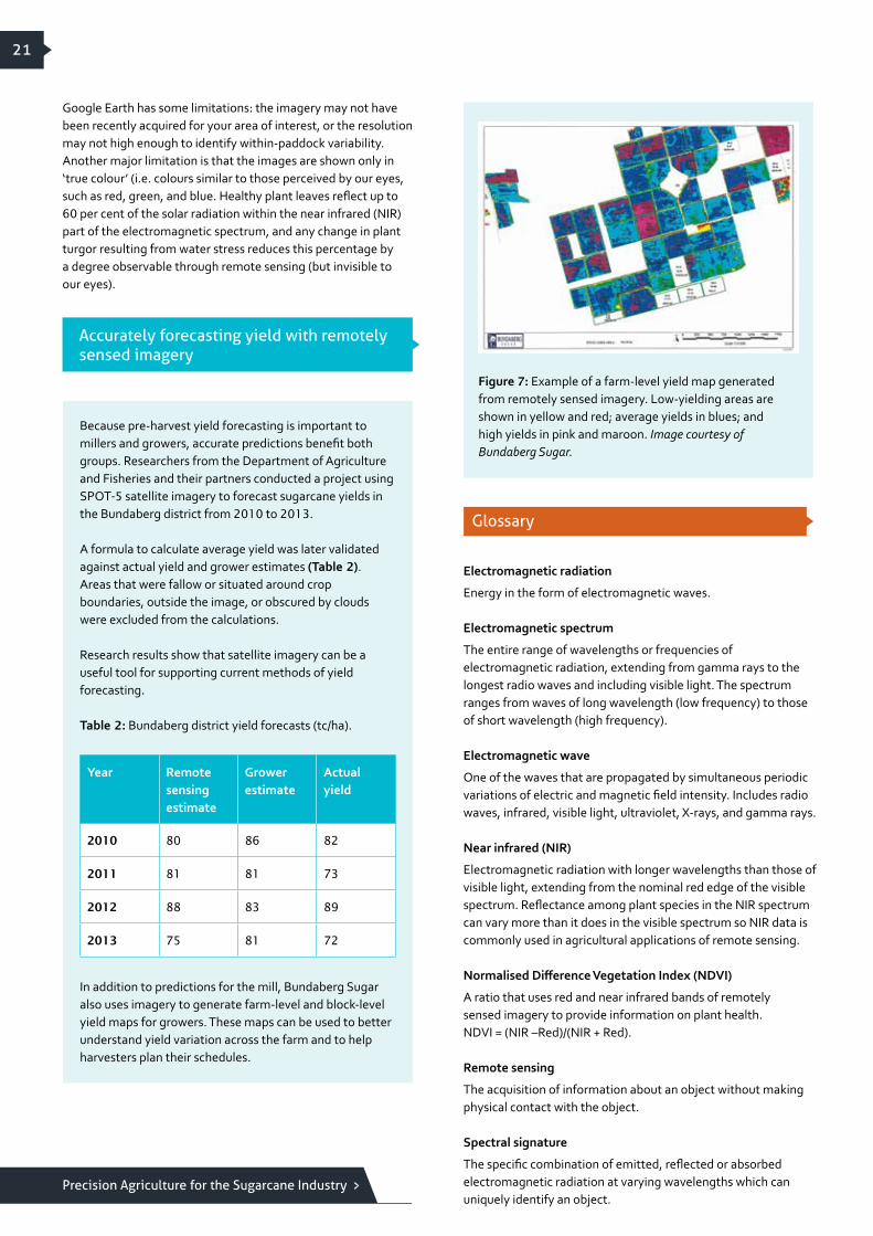
Because pre-harvest yield forecasting is important to millers and growers, accurate predictions benefit both groups. Researchers from the Department of Agriculture and Fisheries and their partners conducted a project using SPOT-5 satellite imagery to forecast sugarcane yields in the Bundaberg district from 2010 to 2013.
A formula to calculate average yield was later validated against actual yield and grower estimates (Table 2). Areas that were fallow or situated around crop boundaries, outside the image, or obscured by clouds were excluded from the calculations.
Research results show that satellite imagery can be a useful tool for supporting current methods of yield forecasting.
Table 2: Bundaberg district yield forecasts (tc/ha).
Figure 7: Example of a farm-level yield map generated from remotely sensed imagery. Low-yielding areas are shown in yellow and red; average yields in blues; and high yields in pink and maroon. Image courtesy of Bundaberg Sugar.
In addition to predictions for the mill, Bundaberg Sugar also uses imagery to generate farm-level and block-level yield maps for growers. These maps can be used to better understand yield variation across the farm and to help harvesters plan their schedules.
Accurately forecasting yield with remotely sensed imagery
Year
Remote sensing estimate
Grower estimate
Actual yield
2010 80 86 82
2011 81 81 73
2012 88 83 89
2013 75 81 72
Electromagnetic radiation
Energy in the form of electromagnetic waves.
Electromagnetic spectrum
The entire range of wavelengths or frequencies of electromagnetic radiation, extending from gamma rays to the longest radio waves and including visible light. The spectrum ranges from waves of long wavelength (low frequency) to those of short wavelength (high frequency).
Electromagnetic wave
One of the waves that are propagated by simultaneous periodic variations of electric and magnetic field intensity. Includes radio waves, infrared, visible light, ultraviolet, X-rays, and gamma rays.
Near infrared (NIR)
Electromagnetic radiation with longer wavelengths than those of visible light, extending from the nominal red edge of the visible spectrum. Reflectance among plant species in the NIR spectrum can vary more than it does in the visible spectrum so NIR data is commonly used in agricultural applications of remote sensing.
Normalised Difference Vegetation Index (NDVI)
A ratio that uses red and near infrared bands of remotely sensed imagery to provide information on plant health. NDVI = (NIR –Red)/(NIR + Red).
Remote sensing
The acquisition of information about an object without making physical contact with the object.
Spectral signature
The specific combination of emitted, reflected or absorbed electromagnetic radiation at varying wavelengths which can uniquely identify an object.
Glossary

22
Yield mapping
Weed sensors Case studies ReferencesCCS sensors
High-resolution soil mapping
Introduction
Variable-Rate Technology (VRT)
PA technologies Global Positioning Systems (GPS) and other Global Navigation Satellite Systems (GNSS)
Geographic Information Systems (GIS)
Remote Sensing (RS)

Yield mapping
23
Yield maps from multiple crop harvests form the basis for many precision-farming decisions. Traditionally, growers know the average crop yield for a paddock. Average yield masks the variability that exists across a field. Although most growers know their fields well and are able to estimate the performance of crops in different parts of the field, yield mapping can transform those estimates into quantitative values that can be more easily used for making decisions.
Knowledge of where productivity varies and the extent of variability on a farm can be combined with information about soils, elevation and farm inputs to understand why yield varies. This information can be used to increase productivity in areas with high yield potential or to increase efficiency and maximise profitability in areas where productivity is unlikely to increase.
Yield maps can be produced using a yield monitor on the harvester or by analysing remotely sensed imagery. Yield monitors generally provide more accurate calculations of actual yield, but can be challenging to calibrate and maintain. Yield maps from imagery can be cheaper and easier to produce than those from monitors. However, at a farm- and block-level, accuracy can be highly variable. Generally, yield maps are more useful at identifying high- or low-yielding areas than actual yield values. Both types of yield maps can be useful if the user knows how to interpret them.
Yield monitors
Yield monitors are crop-yield measuring devices installed on harvesting equipment. The data from the monitor is regularly recorded and stored, along with positional data from a GPS unit. GIS and other software are then used to organise the data and create yield maps.
On a sugarcane harvester, yield monitors are sensors that measure the flow of material in different parts of the harvester. The data are then calibrated against tonnage recorded at the mill. Recent research has evaluated four different types of sensors that can be installed on a sugarcane harvester to provide yield data (Figure 1).
1. Roller opening, to measure volume through the rollers.
2. Chopper pressure, which assumes that the power required to chop cane into billets is proportional to the cane mass.
3. Elevator pressure, which assumes that the power required to move the elevator is proportional to the cane mass.
4. Load cell, in the elevator floor to measure mass.
Precision Agriculture for the Sugarcane Industry
Figure 1: Sugarcane harvester showing locations of different sensors that can be used to create yield maps.
Chopper pressure
Roller openingTopper
Elevator
Chopper system
Optical/duration
Primary cleaning system
Secondary cleaning system
Load cell
Elevator pressure
FeedtrainFinned roller
Knockdown roller
Gathering system
Basecutters

24
All yield monitors that have been studied provide comparable yield data when they are calibrated correctly and when the harvester is operated according to best management practices. It is important to remember that yield monitors do not actually ‘know’ how much sugarcane has been harvested. They measure a surrogate – volume, mass and pressure – which can be affected by factors such as:
• variation in pour rates
• variation in harvester ground speed
• uneven feeding of crops, especially ratoons
• care and maintenance of devices.
Additionally, variations in consignment accuracy at the mill affect the accuracy of processed data. For best results, the yield monitor data should be processed per harvest or when the harvester moves to a new block.
Currently, the only commercially available yield monitor in Australia measures the harvester’s roller opening. When used correctly, this type of monitor can produce accurate results. High and/or varying pour rates can reduce confidence in the monitor’s accuracy and the yield maps generated. A yield monitoring system based on elevator pressure was produced but is no longer available. A prototype chopper pressure monitor that some growers have used effectively is also available. Systems based on the weigh-pad principle are available from Brazil.
Other commercial monitors, along with systems fitted as original equipment on new harvesters, are scheduled to become available soon. Current research in this area is heavily focused on providing the industry with more commercially viable options and a reliable process for creating maps from yield monitor data.
Creating accurate yield maps from yield monitor data requires a certain set of procedures to be followed. The following steps summarise the full protocol presented at the 2013 Australian Society of Sugar Cane Technologists (ASSCT) conference:
• geolocation with GPS and integrated sensors
• digitised, projected block boundaries
• yield monitor calibration per harvest
• logging of yield data at 3-second intervals, or where more frequent logging is used, data thinning to an equivalent of 3-second logging
• removal of errors and aberrant values from yield monitor data based on harvester speeds of 0.75 m/s and zero yields, followed by cleaning of values that are more than three standard deviations from the mean yield
• map interpolation, using statistically viable calculations
• GIS software.
For each mapped block, a standard grid must be defined so that map layers are projected correctly and can be overlaid and compared. This step requires a block boundary that can be obtained via differentially corrected GPS or digitised from aerial imagery. Then a standard grid cell size must be determined; ideally, a pixel size of two metres for most sugarcane blocks.
One issue commonly associated with sugarcane yield mapping is the error introduced to maps from incorrect consignment. Ideally, an electronic consignment system should be used for maximum accuracy. It would also speed up the process of getting data from yield monitors into a usable map.
Figure 3: Example of a yield map, of a 27 ha Burdekin farm block, generated from yield monitor data. Average yield for this block was 176.5 t/ha but actual yield varied by more than 200 t/ha for the block.
Figure 2: Commercial yield monitor (yellow) alongside a research yield monitor (white), both measuring the harvester’s roller opening.
Commercial yield monitors
Creating yield maps from yield monitor data
< 80
80–120
120–160
160–200
200–240
240–280
> 280
Yield (t/ha)

Precision Agriculture for the Sugarcane Industry
25
Sugarcane yield maps can be created from remotely sensed imagery using sets of calculations called algorithms. Different algorithms must be developed to take into account scale (regional vs. farm level), cane lodging, growing conditions, plant variety and other factors that affect reflectance values in the imagery. Field validation is necessary to establish the accuracy of an algorithm when it is being developed. Resulting maps can be used for a variety of purposes, though their accuracy at the block level is not as high as maps produced from yield monitors. In some cases, these maps may be more useful in comparing high- with low-yielding areas than calculating actual harvested tonnes of cane per hectare.
In sugarcane, the most common use of yield maps from remotely sensed imagery has been yield forecasting (see section on remote sensing). These maps have also been used at the farm- and block-level for harvest planning and visual assessments. With the help of consultants and more data layers, some growers have been able to use these maps for more advanced practices, such as developing variable-rate nutrient plans.
Yield maps produced from remotely sensed imagery provide a good alternative to maps produced from yield monitor data when information is needed for a large area, such as the regional-scale yield forecasting, or in areas where yield monitor data are not available.
Figure 4: Example of a regional yield map developed from remotely sensed imagery and overlaid on Google Earth imagery. This type of image can give a good indication of regional trends, and the underlying data can be used for activities such as harvest management and productivity services decisions. Image courtesy of Andrew Robson, UNE-PARG.
Creating yield maps from remotely sensed imagery
Figure 5: A block-level yield map (top) generated from a false colour image and sampling points (bottom). Images courtesy of Andrew Robson, UNE-PARG.
Obtaining reliable yield maps has been an ongoing issue in the sugarcane industry and, in some cases, has prevented the development of true precision agriculture techniques and practices. Accurate yield information can be obtained using available resources if the user follows strict protocols and understands the methodology behind the data. Remember:
Rubbish in = Rubbish out
Current research on yield monitors is focused on developing monitoring and mapping techniques that can be more readily adopted by a wide audience. This will be accomplished through collaboration and with commercial equipment and service providers, as well as exploring improved consignment and yield monitor calibration options. Researchers are also working to refine algorithms for production of yield maps from imagery at different scales and in different regions.
The future of yield mapping
20–31
31–42
42–53
53–64
64–75
75–85
85–96
96–107
TCH
120–158
90–120
60–90
30–60
0–30
TCH

26
The most widespread use of yield monitors in the sugar industry has been in the Herbert, with Herbert Cane Productivity Services Limited (HCPSL) leading the way. Currently, 25 out of 60 harvesters in the region are fitted with Solinftec yield monitors that measure the roller openings and speed to estimate yield.
Throughout the harvesting season the monitors send raw data to a server where it is intersected with the cane block layer and then interpolated using spatial analysis algorithms. The yield maps are created nightly via an automated process. As a result, around 50 per cent of the entire district’s area is mapped each year. These maps are used for a variety of purposes.
Growers can access yield maps for their own farm online through the Herbert Resource Information Centre (HRIC) where they can use them to visually assess performance, and evaluate the impacts of management practices. Some more-advanced growers are working with agronomists to analyse the maps along with other data to develop variable-rate prescriptions.
Figure 6: Sample yield map accessible through the HRIC information portal. These maps are produced yearly via an automated process and can be used by growers and productivity services for a variety of purposes.
Additionally, HCPSL uses the maps regularly to meet their objectives. Yield maps can show metre-by-metre variety strip performance without the need for expensive on-ground field trials. The yield monitors provide data to compare varieties planted side-by-side in the same block, in terms of biomass entering the harvester to help identify the most productive varieties. They also use yield maps to assess inputs for trials evaluating products, such as controlled-release fertiliser, mud and ash. The maps provide information on harvested strips showing metre-by-metre yield for varying treatments.
Yield monitoring in the Herbert: a whole system approach
While the mills might not use individual yield maps, the data logged by the harvesters helps them with harvest management, including things like harvest equity, bin deliveries, harvest performance reports, and analysis of pour rate versus ratoonability of a crop.
Michael Sefton, HCPSL Spatial Systems and PA Coordinator, acknowledges that mapping yield for such a large area is challenging, and the data is more accurate for some areas than others. At the same time, he can see the current and potential benefits of yield monitoring and wants to continue to refine the system.
In the future, Sefton would like to see a more holistic approach to yield mapping throughout the industry. He believes that yield maps should eventually be more fully integrated with other spatial data, such as elevation and soil maps and other business processes. He would also like to see more agronomy and extension services using these tools so that growers can receive the best advice possible.

27
High-resolution soil mapping
Geographic Information Systems (GIS)
Weed sensors
PA technologies
Case studies ReferencesCCS sensors
Yield mappingRemote Sensing (RS)
Variable-Rate Technology (VRT)
Global Positioning Systems (GPS) and other Global Navigation Satellite Systems (GNSS)
Introduction

28
Above: A Veris 3100 taking measurements of soil electrical conductivity by injecting an electrical current into the soil and measuring the changes in return voltage. The system also includes a GPS receiver and an on-board data logger. Note that the four coulters on the Veris must make contact with the soil to get accurate readings.
Above: The EM38 (insert) is a handheld sensor that measures how much soil resists the flow of electricity. For rapid data collection over a large area, this instrument can be pulled on a metal-free ‘sled’ and used with a GPS and data logger. Since the EM38 does not need to make contact with the soil, it can easily collect data through a trash blanket, as pictured here.
Conversely, the EM38 is an electromagnetic induction sensor that measures how much the soil conducts the flow of electricity. This instrument does not have to make contact with the soil surface to take an accurate reading.
As we saw in the previous section, a yield map can show crop variability in the field, but it does not give reasons for that variability. One important piece of information that can help growers better understand underlying reasons for differences in yield is high-resolution soil data. In a typical 1:100,000 soil survey, one unit equals 80 hectares, which is not enough detail for precision agriculture purposes. Different soil-sensing systems can provide more-detailed soils information suitable for PA, including soil-apparent electrical conductivity (ECa) mapping and gamma radiometrics, which are discussed here.
One map layer that is commonly used for site-specific crop management is a map of soil-apparent electrical conductivity (ECa), sometimes called an ‘EC map’ or ‘EM map’.
Soil ECa
Soil ECa is a measurement of a soil’s ability to conduct electricity. It is useful because it can indicate physical and chemical properties, such as:
• clay content/soil texture
• moisture content
• salinity.
Because ECa is affected by a variety of properties, it should always be used in combination with soil samples collected for laboratory analysis.
An ECa map can serve as a guide for selecting soil sample locations to give a more representative set of samples than traditional grid sampling.
Measuring ECa
Currently, two instruments are used to obtain ECa soil data in Australian sugarcane. The Veris 3100 is a commercial instrument that connects to the back of a truck or tractor and runs over the soil surface. The tines must be in contact with the soil to measure the electrical conductivity of the soil.
High-resolution soil mapping
Soil-apparent electrical conductivity (ECa)

Precision Agriculture for the Sugarcane Industry
29
The EM38 and Veris instruments produce similar results for precision agriculture purposes.
With both instruments, soil ECa may be measured over two different depths ranges: shallow (~0–30 cm for Veris, and 0–50 cm for EM38) and deep (~90 cm for Veris, and 0–150 cm for EM 38).
When the Veris 3100 or EM38 are used in conjunction with a GPS, maps of soil ECa can be created to show areas of relatively high and low conductivity in a paddock or on a farm. Because numerous soil properties influence ECa, high-resolution soil data cannot be used to determine which specific soil properties are there unless they are calibrated with results from soil samples across the mapping range.
ECa maps provide information for identifying ideal locations for soil samples that more accurately represent soil variability than traditional sample patterns, such as grids. Samples can be strategically placed across a range of ECa values. This method may result in higher concentrations of samples in some areas, but samples will represent a wider range of soil conditions (Figure 1).
ECa and precision agriculture
The pattern of ECa variation across a paddock or farm is often similar to that seen in yield maps or in remotely sensed imagery and, therefore, forms the basis for understanding the main drivers of yield variation. Generally, it is best to take measurements when the soil moisture profile is damp; it should not be fully saturated or dry. As clay content increases, the ability of a soil to store moisture increases, as does the cation exchange capacity (CEC) (which increases the soil’s ability to store nutrients).
ECa data should be combined with other information, such as elevation maps and crop yield maps, for a better understanding of why different areas are more or less productive. This can help with creating prescriptions for inputs, such as gypsum, lime, and fertiliser applications. Figure 1 on Page 14 shows an example of ECa information overlaid with elevation and yield data to develop management zones on a Burdekin cane farm.
Obtaining an ECa map
The easiest way to obtain an ECa map is to hire a contractor (costs start at about $35/ha). Local productivity services should have information about ECa maps that have already been created, so check with them before buying new maps.
The following manual for ECa mapping was produced in 2011. It provides detailed information about how to produce maps and what they can be used for:
• Operations manual for apparent soil electrical conductivity mapping: A guide to collecting, analysing, and interpreting soil ECa data in precision sugarcane agriculture.
www.sugarresearch.com.au/icms_docs/188116_Operations_manual_for_soil_electrical_conductivity_mapping.pdf
Gamma radiometrics is the measurement of natural gamma ray emissions, primarily from the top 40 cm of soil or rock. Often this figure can provide information about the parent material of the soil that can be related to soil types across the region or paddock.
Gamma rays are emitted as high-energy, short wavelength, electromagnetic radiation. They are part of the natural radioactive decay process. They can be detected by sensors because they can travel a reasonable distance in air.
Figure 1: ECa map showing variation across a paddock and strategically placed soil sample locations (blue triangles) to cover the range of ECa values.
Gamma radiometrics
< 120
120–140
140–160
160–180
180–200
200–220
> 220
Soil sampling locations
ECa deep (mS/m)

30
Gamma radiometrics in precision agriculture
Useful relationships have been found between gamma radiometrics and soil properties (particularly plant-available potassium), texture of the top soil, unsaturated hydraulic conductivity, bulk density, organic carbon, Colwell phosphorus, and pH. Like the use of ECa measurements, these relationships are specific to the areas where they are developed and cannot be used universally.
Measuring gamma radiation
Potassium (K), uranium (U) and thorium (Th) are the three major elements in soil that have naturally occurring isotopes that emit gamma rays as they decay. These can be measured in different windows of the energy spectrum or as a total count across a specified energy spectrum range. Gamma rays are measured ‘on the go’ by a gamma radiometer, and can be measured simultaneously with ECa.
Fifty per cent of gamma rays detected above the soil surface have been emitted from the top 10 cm of soil, and 90 per cent from the top 40 cm of soil. Gamma rays from soil deeper than 50 cm are blocked by soil above. They can also be blocked by increasing soil moisture in the top soil. Generally, vegetation cover has little effect on measurements.
Gamma radiometrics in sugarcane
When researchers trialled gamma radiometrics on a limited number of sugarcane blocks, they had some success establishing relationships between gamma radiometrics and other soil properties. To date, gamma radiometrics has not been used outside a research setting in sugarcane.
Cation exchange capacity (CEC)
The maximum quantity of total cations that a soil is capable of holding, at a given pH value, available for exchange with the soil solution. In general, the higher the CEC, the higher the soil fertility.
EM38
An electromagnetic induction sensor that measures soil resistivity without making contact with the soil.
Gamma radiometrics
The measurement of natural gamma ray emissions.
Gamma ray
Electromagnetic radiation of extremely high frequency and, therefore, high energy per photon.
Soil-apparent electrical conductivity (ECa)
A measure of how much the soil conducts electricity.
Glossary
Soil resistivity
A measure of how much the soil resists or opposes the flow of electricity.
Veris 3100
A soil-mapping instrument that measures electrical conductivity of the soil by one pair of coulter-electrodes injecting a known voltage into the soil, while another pair measures the drop in that voltage.

31
Variable-rate technology
Geographic Information Systems (GIS)
Weed sensors
PA technologies
Case studies ReferencesCCS sensors
Yield mappingRemote Sensing (RS)
Global Positioning Systems (GPS) and other Global Navigation Satellite Systems (GNSS)
Introduction
High-resolution soil mapping

32
Variable-rate technology (VRT) is the range of equipment allows fertiliser, chemicals, lime, gypsum, irrigation water and other farm inputs to be applied at different rates across a field, and not just between fields, without manually changing rate settings on equipment or having to make multiple passes over an area.
Variable-rate application (VRA) can range from the simple control of flow rate to a more complex management of rate, chemical mix and application pattern. VRA can match changes in crop-yield potential with specific input rates, resulting in a more efficient system and minimising potential environmental impacts.
VRT can be used to deal with spatial variability between paddocks or between management zones/classes. There are two types of VRT:
1. Map-based control: a map of application rates is produced for the field prior to the operation.
2. Real-time control: decisions about the rates to apply in different locations are made using information gathered during the operation. It requires sensors to detect necessary information ‘on the go’ and is usually designed for a specific job, such as herbicide application.
Here we will focus on map-based control, which is currently more commonly used in sugarcane. Requirements of VRA systems:
• Prescription maps to provide site- or zone-specific input rates. These types of maps are generally created using Geographic Information Systems (GIS) software.
• Global Navigation Satellite System (GNSS), such as GPS, to help the applicator interpret the prescription map.
• Variable-rate capable machinery (sprayer, spreader, etc.). Though it is often possible to adapt existing machinery, methods for doing so vary from one machine to another.
• A controller that uses application maps to vary the rate of input. Many tractor navigation systems incorporate VRA map-reading and control-signalling ability.
The greatest benefits of VRA are found in areas with high variability of the issue of interest (soil fertility, weed growth, etc.). The economic benefits of VRA can include cheaper inputs
Variable-rate technology
Benefits of variable-rate application
Variable-rate equipment
Controllers for three separate compartments
Image 1: Example of a variable-rate fertiliser box with three compartments that are controlled separately by the three black controllers to the right of the tyre.
and better crop yield. Use of VRA can also have positive environmental implications by more closely matching inputs to crop needs, thus reducing environmental run-off.
VRA requires a high level of data management and interpretation. Benefits of VRA are generally higher when:
• the amount of spatial variation is larger
• the pattern of variability is more coherent patches (fewer rate changes needed)
• variability patterns are stable over time
• the cost of inputs is relatively high (e.g., benefits are higher for VRA of gypsum than for VRA of nitrogen).
Because there are different types of variable-rate equipment, it is important to carefully consider what is needed before buying or modifying equipment. Also, consider that liquid fertilisers can usually be applied more accurately at varying rates than granular. Some applicators can vary the rate of one product only. However, in many cases, crop needs will vary across a block for different nutrients. More flexibility can be achieved by using a fertiliser box with multiple compartments (Image 1). This fertiliser box has three compartments that are controlled separately, as indicated by the three black controllers to the right of the tyre.
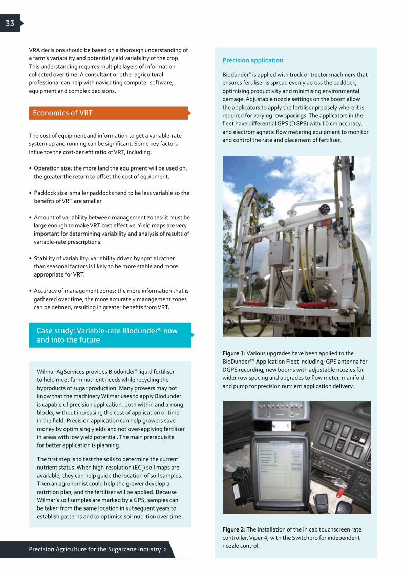
Precision Agriculture for the Sugarcane Industry
33
VRA decisions should be based on a thorough understanding of a farm’s variability and potential yield variability of the crop. This understanding requires multiple layers of information collected over time. A consultant or other agricultural professional can help with navigating computer software, equipment and complex decisions.
The cost of equipment and information to get a variable-rate system up and running can be significant. Some key factors influence the cost-benefit ratio of VRT, including:
• Operation size: the more land the equipment will be used on, the greater the return to offset the cost of equipment.
• Paddock size: smaller paddocks tend to be less variable so the benefits of VRT are smaller.
• Amount of variability between management zones: it must be large enough to make VRT cost effective. Yield maps are very important for determining variability and analysis of results of variable-rate prescriptions.
• Stability of variability: variability driven by spatial rather than seasonal factors is likely to be more stable and more appropriate for VRT.
• Accuracy of management zones: the more information that is gathered over time, the more accurately management zones can be defined, resulting in greater benefits from VRT.
Economics of VRT
Wilmar AgServices provides Biodunder® liquid fertiliser to help meet farm nutrient needs while recycling the byproducts of sugar production. Many growers may not know that the machinery Wilmar uses to apply Biodunder is capable of precision application, both within and among blocks, without increasing the cost of application or time in the field. Precision application can help growers save money by optimising yields and not over-applying fertiliser in areas with low yield potential. The main prerequisite for better application is planning.
The first step is to test the soils to determine the current nutrient status. When high-resolution (ECa) soil maps are available, they can help guide the location of soil samples. Then an agronomist could help the grower develop a nutrition plan, and the fertiliser will be applied. Because Wilmar’s soil samples are marked by a GPS, samples can be taken from the same location in subsequent years to establish patterns and to optimise soil nutrition over time.
Case study: Variable-rate Biodunder® now and into the future
Precision application
Biodunder® is applied with truck or tractor machinery that ensures fertiliser is spread evenly across the paddock, optimising productivity and minimising environmental damage. Adjustable nozzle settings on the boom allow the applicators to apply the fertiliser precisely where it is required for varying row spacings. The applicators in the fleet have differential GPS (DGPS) with 10 cm accuracy, and electromagnetic flow metering equipment to monitor and control the rate and placement of fertiliser.
Figure 1: Various upgrades have been applied to the BioDunder™ Application Fleet including; GPS antenna for DGPS recording, new booms with adjustable nozzles for wider row spacing and upgrades to flow meter, manifold and pump for precision nutrient application delivery.
Figure 2: The installation of the in cab touchscreen rate controller, Viper 4, with the Switchpro for independent nozzle control.

34
A touchscreen control panel controls VRA, auto steer and automatic remote data download for liquid application data. Machinery is also able to apply reduced rates to buffer zones and automatically switch off boom or individual nozzles where a field boundary layer is available. Application performance has been reported as being highly precise, with a variation of +/-50 L over a 12,000-litre load.
Data for each application, including product type, target rate, actual rate, time, total area, total volume, row spacing and elevation, is recorded and compiled in a GIS program to create an application map record. Currently, data processing is a complex process, and Wilmar is working with Herbert Resource Information Centre (HRIC) to automate the procedures and increase efficiency.
Figure 3: Example of Precision Liquid Fertiliser Application map indicating different product types and rates between blocks on farm. All application sessions were manually compiled and analysed to identify product type, time of application, rate of application.
Within-block variable rate
Currently, it is common for Biodunder application to vary between blocks, but not within blocks. This is primarily due to a lack of data, such as yield maps, to develop full VRA prescriptions. The Biodunder application system is capable of variable-rate product control based on application maps that are uploaded into the unit. They also have the capability to capture meteorological data from selected weather stations and offer multi-product control, though this hasn’t been implemented on a commercial scale.
Wilmar continues to work towards complete variable-rate precision application and believes that this will provide great value to the industry, including growers, millers, consultants and government bodies. Future collaboration of industry bodies is required to make this happen and will benefit all involved.
Variable-rate irrigation (VRI)
Variable rate irrigation (VRI) is the application of irrigation water at rates that match the needs of individual areas within fields. Variable soils and topography result in variable water-holding capacities throughout a farm that are not addressed by most irrigation systems. VRI systems are designed to automatically adjust water application rates to match the needs of the field. Soil-moisture probes can help identify and manage the effectiveness of VRI systems.
In practice, some VRI plans have been designed to meet irrigation needs that vary due to inefficient farm design. For example, in some cases, irrigation equipment traverses numerous paddocks at different crop stages, including fallow fields, resulting in varying water needs. Situations like this may be addressed more cost effectively by consolidating paddocks and improving overall farm design than by investing in VRI. Laser levelling could reduce the need for VRI in some cases as well.
Centre pivot VRI
Most VRI work has been done on centre pivots, though other overhead systems may also be capable of applying VRI. To determine the potential usefulness of VRI, zones can be established using the same information as other variable-rate applications, i.e. soil maps and topography. The more variability there is within a field, the greater the potential benefit from VRI. There are two basic types of centre pivot VRI: speed control and zone control. Costs of both systems should be weighed against benefits related to the amount of in-field variability when making decisions about implementation.
Speed control is a simple form of VRI in which the pivot area is divided into pie sections with rates set to the average needs of each section. The pivot travel speed is adjusted manually or through the control panel for each section. Pressure and flow rate remain constant while application depth increases or decreases. This is a low-cost way to match irrigation depth to soils, though effectiveness will vary depending on the patterns of soil variation in the field.
Zone control is a more advanced VRI system that involves control of individual sprinklers or banks of sprinklers along the pivot span, using pulsing valves. It allows water management on a much finer scale and is not limited to the pie shape, which may not match the variability patterns of the field. Zone control can accommodate an essentially unlimited number of zones to meet soil and crop needs; however, it is more costly and may require more intensive management.
Figure 4: Example of VRI speed control (left) and zone control (right) for a centre pivot irrigating a field with variation in irrigation needs established by the soil map in the centre. Image courtesy of CropMetrics, www.cropmetrics.com

35
Weed sensors
Geographic Information Systems (GIS)
PA technologies
Case studies ReferencesCCS sensors
Yield mappingRemote Sensing (RS)
Global Positioning Systems (GPS) and other Global Navigation Satellite Systems (GNSS)
Introduction
High-resolution soil mapping
Variable-Rate Technology (VRT)

36
Image 1: Tractor fitted with three WeedSeeker® sensors and a custom spray shield to confine herbicides to the desired area.
WeedSeeker has been tested in a variety of soil types with different weed patterns. Some guidelines describing the most effective use of this technology are presented.
Weed type and size
WeedSeeker sensors work well on weeds or grasses that:
• are bigger than 60 mm in diameter
• are green or turning yellow because they are mature
• have a spreading habit.
Weed sensors are used to minimise the amount of herbicide applied to fallow paddocks, or to crop inter-rows when used with spray hoods. Precision spraying has the potential to improve weed management by targeting the weed, not the crop. In addition to reducing weeds, precision spraying has economic benefits by reducing total herbicide use and providing flexibility in weed management by enabling a wider variety of herbicide options. Minimising herbicides also reduces off-site run-off.
There are two general classes of weed sensors:
1. sensors that can distinguish ‘green from brown’, or weeds from bare ground or trash
2. sensors that can distinguish ‘green from green’, or weeds from crops.
We will focus on the first type because the second is still in development and is not commercially available for sugarcane.
WeedSeeker® sensors are the only ‘green from brown’ sensors that have been studied in sugarcane. They are used to identify weeds and to spray only where the herbicide is needed, not bare ground. They have been tested for effectiveness on various soil types and for different types of weeds, and have been found to be useful and cost-effective under some circumstances.
The WeedSeeker product works by assessing the ratio difference of red and near infrared (NIR) image reflections of vegetation and background. Sensors with nozzles are attached to the sprayer. The sensors use optical recognition to detect the green leaves from the different-coloured background trash or bare soil. When a green leaf is detected, the sensor then triggers a directed spot spray through the nozzle that targets the green leaves.
In sugarcane farming systems where non-selective herbicides are used, spray shields or hoods allowing inter-row spraying within the sugarcane crop are necessary. SRA researchers have designed a prototype spray hood to protect the crop by deflecting the lower leaves because the sensors do not discriminate between green sugarcane leaves and green weeds. Additionally, the hood protects the crop from herbicide drift.
Weed sensors
WeedSeeker® technology
WeedSeeker use in sugarcane

Precision Agriculture for the Sugarcane Industry
37
WeedSeeker sensors do not perform well on weeds or grasses that:
• are smaller than 60 mm in diameter (many misses occur even on highest sensitivity settings)
• have an upright habit with narrow leaves, especially nutgrass or sedges, unless they are in a solid clump larger than 60 mm in diameter.
Image 2: Sensors accurately detect clumps of weeds, such as paspalum, in sugarcane inter-rows (top), but generally miss narrow-leaved weeds, such as nutgrass (bottom).
Weed distribution
Weed distribution can affect the economics of the WeedSeeker. The sensors work effectively on scattered clumps of weeds, such as isolated clumps of paspalum. When there is an even distribution of small weeds across the field, such as emergence of blue top, the WeedSeeker sensors trigger most of the time, even if the total weed coverage is low. If the sensors trigger continuously or near continuously, the benefit of the technology is not realised. This feature makes the sensors more economical on isolated big clumps of weeds than on an even distribution of small weeds.
Effect of background
Before every use, WeedSeeker sensors need to be calibrated for the background where the weeds are. The sensors perform well on any soil background as long as it is uniform, e.g., freshly tilled soil in fallow or plant cane, or a fresh trash blanket on a ratoon. Any changes in soil colour or presence of dead stubble will potentially trigger the nozzles to misfire, e.g., minimum tillage system). In these situations, adjusting calibration settings according to manufacturer specifications is unsatisfactory because either many weeds are missed or many misfires occur.
Current commercially available shield designs have limitations when used with WeedSeeker. The following common problems have been observed when fitting and adapting commercial shields to the WeedSeeker:
• drift escape that can damage crops
• low-pressure turbulence from dust/spray mist that can interfere with optics
• cane leaf detected by the sensors that cause misfires
• shields that may not accommodate three or four sensors and nozzles at the correct settings (height, spacing, alignment of nozzles to sensors).
Before investing in this technology, growers should consider the five limitations represented below. Failure to satisfy one or more of these limitations could result in a lack of economic benefit from the WeedSeeker technology.
To be economical in sugarcane, the WeedSeeker technology must be used in situations that combine:
• an even background so it triggers the least number of misfires
• weed size larger than 60 mm in diameter (no nutgrass or sedges)
• weed distribution that is primarily isolated clumps to avoid sensors triggering continuously.
Researchers calculate that the WeedSeeker sprayer is economical if it sprays less than 42 per cent of the total spray area and achieves an effective weed kill without cane damage.
Estimated costs of precision spraying components (2014)
• WeedSeeker sensors: $1300–$1500 each (minimum of three required per inter-row).
• Shield construction, including frame, spray heads and materials: $2100 each.
• WeedSeeker controller: $2500 (one for the entire sprayer).
Limitations of commercial shields
Cost effectiveness

38
• Less than 1000 ha • More than 1000 ha
• Uniform soil colour• Fresh trash blanket
• More than 42% • Less than 42%
• Big clumps of weeds
• Shield specially designed for Weedseeker® technology
• Inadequate shield
• Soil cover variations• Stubble• Weathered trash
• Small scattered weeds
• Nutgrass
TYPE OF SHIELD
Une
cono
mic Econom
icHECTARES SPRAYED
ANNUALLY
BACKGROUND TYPE
WEED COVERAGE
WEED DISTRIBUTION
Figure 1: Decision support tree for use of the WeedSeeker precision sprayer.
More information about the WeedSeeker technology and its use in sugarcane is available at www.sugarresearch.com.au/page/Growing _cane/Weeds/Spraying_systems/Weedseeker_technology
For most individual growers, investing in WeedSeeker technology is not practical because of the current cost. For this reason, researchers worked with spraying contractors to determine a realistic number of hectares that must be sprayed yearly to make the technology cost effective and to establish a cost for the shield used for inter-row spraying. Under the established circumstances, researchers determined that a contractor would pay off the WeedSeeker technology within three years if they sprayed 3000 to 4000 ha within that time period.
Shielded spraying in ratoon cane
Two growers trialled the WeedSeeker using modified shields but had limited success due to problems with the shields. Researchers designed a shield especially for use with the WeedSeeker technology, which has some limitations when used with the manufacturer’s sprayer recommendations, but has proven effective under certain circumstances. Table 1 compares different scenarios for spraying costs using the WeedSeeker in ratoon cane. It was cost effective when the area sprayed was 30 per cent or less.
An economic evaluation of WeedSeeker in fallow fields compared with boom spraying
Researchers compared the WeedSeeker technology to boom spraying in fallow fields with different soil colours. They found that the technology could be a cost-effective option for contractors spraying large areas under optimal conditions.
The study used an estimate of $30/ha for boom spraying versus $42/ha for the WeedSeeker, and looked at the use of Roundup PowerMax ($8 at 2 L/ha) and Liase ($2.15 at 2 L/100 L). Under all conditions, the WeedSeeker used less chemicals than the boom sprayer, but the additional cost of the technology was offset only on dark soils, which had fewer misfires (see Table 2).
Economic viability of WeedSeeker technology in sugarcane
More information about WeedSeeker use in sugarcane
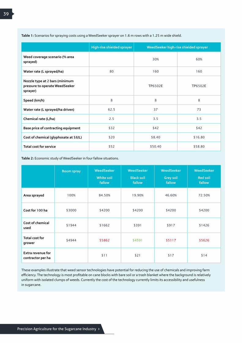
Precision Agriculture for the Sugarcane Industry
39
These examples illustrate that weed sensor technologies have potential for reducing the use of chemicals and improving farm efficiency. The technology is most profitable on cane blocks with bare soil or a trash blanket where the background is relatively uniform with isolated clumps of weeds. Currently the cost of the technology currently limits its accessibility and usefulness in sugarcane.
Table 2: Economic study of WeedSeeker in four fallow situations.
High-rise shielded sprayer WeedSeeker high-rise shielded sprayer
Weed coverage scenario (% area sprayed)
30% 60%
Water rate (L sprayed/ha) 80 160 160
Nozzle type at 2 bars (minimum pressure to operate WeedSeeker sprayer)
TP6502E TP6502E
Speed (km/h) 8 8 8
Water rate (L sprayed/ha driven) 62.5 37 73
Chemical rate (L/ha) 2.5 3.5 3.5
Base price of contracting equipment $32 $42 $42
Cost of chemical (glyphosate at $8/L) $20 $8.40 $16.80
Total cost for service $52 $50.40 $58.80
Boom spray
WeedSeeker
White soil fallow
WeedSeeker
Black soil fallow
WeedSeeker
Grey soil fallow
WeedSeeker
Red soil fallow
Area sprayed 100% 84.50% 19.90% 46.60% 72.50%
Cost for 100 ha $3000 $4200 $4200 $4200 $4200
Cost of chemical used
$1944 $1662 $391 $917 $1426
Total cost for grower
$4944 $5862 $4591 $5117 $5626
Extra revenue for contractor per ha
$11 $21 $17 $14
Table 1: Scenarios for spraying costs using a WeedSeeker sprayer on 1.6 m rows with a 1.25 m wide shield.

40
CCS sensors
Weed sensors Case studies References
High-resolution soil mapping
Introduction
Variable-Rate Technology (VRT)
PA technologies Global Positioning Systems (GPS) and other Global Navigation Satellite Systems (GNSS)
Geographic Information Systems (GIS)
Remote Sensing (RS)
Yield mapping

CCS sensors
41
Sugarcane quality, measured as commercial cane sugar (CCS), is an important factor in sugar production. Currently, there is no way to reliably measure sugarcane quality in the field. If there were, harvesting could be scheduled to optimise sugar value. Availability of infield CCS values would also allow production inputs and harvest schedules to be optimised.
Research has not been able to establish a link between yield and CCS, but many PA activities focus on optimising yield without understanding potential impacts on CCS. Research has found CCS to have an impact on income of 20–25 per cent on trial blocks (with variation in yield accounting for the remaining 75–80 per cent). This finding indicates that the ability to measure CCS in the field would be a valuable tool to enable more accurate management to maximise profits.
Currently, CCS can be measured only in a lab – a complex and time-consuming processes. Additionally, these CCS measurements require the use of juice samples that are not readily available in the field. Other industries have successfully used spectrometers for infield quality measurements. Spectrometers measure properties of light and may include near infrared (NIR) and other non-visible wavelengths.
In the future, researchers would like to develop a prototype CCS sensor to increase the density of CCS data that can be collected in the field. This process would enable them to produce more-detailed maps to determine whether CCS patterns are stable over time and to evaluate how this information could improve farm management to maximise profits.
Precision Agriculture for the Sugarcane Industry

42
Case studies
Weed sensors References
High-resolution soil mapping
Introduction
Variable-Rate Technology (VRT)
PA technologies Global Positioning Systems (GPS) and other Global Navigation Satellite Systems (GNSS)
Geographic Information Systems (GIS)
Remote Sensing (RS)
Yield mapping
CCS sensors

Case studies
43
There are interesting case studies of sugarcane growers who have incorporated PA tools and technologies into their farm management systems. Each grower’s needs are different and, as a result, the tools that they use vary with factors such as farm size, landscape, irrigation requirements, and personal goals and preferences. We have attempted to highlight a range of grower types, but there is no one-size-fits-all prescription for PA, and PA tools are just part of an overall farm management strategy.
Leading growers in PA have some things in common. For example, they tend to be computer literate, use GPS technology, routinely test soils and keep good farm records. They recognise that there is always room for improvement and they are not afraid to try new things. It is intended that the following examples will help growers and others in the sugar industry to see what is possible and perhaps inspire new ideas as well.
Canegrower Bryan Granshaw has spent many years figuring out how to maximise the efficiency and profitability of his farming system. But one thing he hasn’t been able to figure out is why more growers in this industry haven’t adopted recommendations that they paid researchers millions of dollars to develop. Bryan has hosted numerous international visitors at his Dalbeg farm who, like Bryan, are benefiting from the development of improved farming systems.
Improvements include the basics, such as controlled traffic (CT), minimum till, green harvesting, and legume fallows. In addition, Bryan has added practices, such as modern farm recording systems, yield monitoring, variable-rate application of inputs, and water recycling to fine-tune his system.
It all starts with good planning, and that’s what he has done, converting his farm, block by block, from 1.5 m rows to 2 m CT rows. Each block has been laser levelled, apparent electrical conductivity of the soils has been mapped, and accompanying samples marked using a GPS to provide a base layer of information. Bryan also uses a yield monitor on the harvester that he shares with his father and brother to improve his understanding of his farm’s productivity by pinpointing which areas are performing well and where he needs to make changes.
Precision Agriculture for the Sugarcane Industry
Bryan Granshaw: the new farming system
These changes have paid off. Bryan uses farm management software to analyse maps, create variable-rate prescriptions, track costs (tractors, harvesting, hauling, fertiliser, chemicals, and labour) and keep a record of day-to-day activities, such as application of chemicals, fertiliser and water. As well as helping him make precision farming decisions, the software helps him to manage his farm finances.
Bryan is now able to apply variable-rate gypsum to maximise soil health while minimising cost. And the green trash blanket helps prevent the gypsum from blowing away so he gets maximum bang for his buck. He also applies variable-rate liquid fertilisers and herbicides, which saves money and optimises production.
For example, a shielded spray unit his brother, Terry, installed allows him to use less expensive knock-down chemicals under the shields, which reduces the use of expensive residual herbicides and drastically reduces the chance of off-site impacts. He saves 35 per cent of the more expensive selective herbicide compared to using a conventional flat boom. In addition, the GPS-controlled system allows him to spray at two different rates with two different chemicals in one operation and with greater precision. This system maintains application rates even when the tractor speed slows towards the end of the block, and the spray system will turn off automatically when it crosses a field boundary.
One thing that has helped all of the Granshaws succeed with their new farming system is their willingness to modify equipment to suit the way they want to farm, rather than letting equipment manufacturers decide how they should farm. As Bryan says, ‘If people didn’t try something different, we would still be riding horses and not driving cars.’
Granshaw shares the ups and downs of his farming experiences on his blog www.bryan-granshaw.blogspot.com.au
Above: Bryan and Terry Granshaw in Dalbeg, Ayr, North Queensland.

44
Phil Deguara: taking the long view
If there’s one thing that Phil Deguara knows, it’s that change takes time. Although he and his father John bought their first GPS unit 10 years ago, they are still in the process of transitioning to a complete precision system. But the benefits they have noticed along the way have been worth the effort and the wait.
Phil and John farm a 250-ha block at Brightley, west of Mackay. Phil also leases 25 ha at Eton. They initially bought a GPS to move from a 1.5 m system with full cultivation to a 1.9 m controlled-traffic system with zonal cultivation.
The transition has taken time and, in some areas, has made the Deguaras rethink their farm design. Elevation maps from the GPS have helped them determine whether blocks could be joined to increase row length and also whether blocks needed to be laser levelled. The entire farm had soil electrical conductivity (EC) and elevation mapped, and Farmacist consultants have produced yield potential maps from remotely sensed imagery.
Satisfied with the farm layout, Phil and John have moved on to more complex management activities, including variable-rate application (VRA) of nutrients. Working with Farmacist as part of Project Catalyst, the Deguaras have used EC maps to identify poor soils on trial blocks and reduce N in these areas without reducing yield. This application method could save 9 tonnes of urea or about $6000 per year over the whole farm. They are also looking at increased N rates in high-yielding areas to further increase yield. On the trial blocks, their N rates have varied from 90 kg/ha up to 230 kg/ha. If they continue to see positive results, they plan to expand the VRA across the entire farm (Figure 1, Image C). Phil also uses the detailed soil information for VRA of mill ash.
C
Figure 1: The Deguaras’ VRA N program is based on high-resolution soil maps, soil samples and estimates of yield potential. Image A gives an example of a map of soil-apparent electrical conductivity (ECa) (top), where ESP refers to Exchangeable Sodium Percentage, and resulting yield zones (bottom). Image B illustrates the pattern of variable-rate N and the lack of impact on yield in poor soils. Image C illustrates a proposed whole-farm variable-rate N program that the Deguaras plan to use if current trial paddocks continue to produce desirable results. Images courtesy of Farmacist Pty Ltd.
A
B
Above: Eton grower Phil Deguara with the tractor he has modified with a variable-rate valve that is compatible with multiple implements.

Precision Agriculture for the Sugarcane Industry
45
Because they own most of their own equipment, the Deguaras have been able to make modifications that suit their farming system. For example, Phil has modified a tractor with a variable-rate valve that can run multiple implements, including a spray tank, fertiliser box, seeder and mill mud spreader.
Phil says that with technology becoming more affordable and easier to use, it is also possible to coordinate precision farming with contractors. He is able to lend a GPS unit to his harvesting contractor to maintain his controlled-traffic system, and he can put prescription maps onto a thumb drive (aka flash drive or USB stick) to share with other contractors who have compatible equipment.
In addition to using technology, the Deguaras have implemented other changes such as a legume fallow, and installing drains to manage waterlogging and sodicity problems. Phil tries to maintain a big-picture view of what will help them reach their goals of increasing yield in the areas with the highest potential, and reducing inputs while maintaining yields in other areas.
Surprisingly, Phil doesn’t spend a lot of time on a computer. The initial setup of these systems took extra time, but now that they are in place he has plenty of time to spend in the field and in the shed. His advice to other growers getting started with PA is to take things one step at a time. Phil also says that they wouldn’t have been able to cover some of the initial costs of PA gear and advice without the help of programs such as Reef Rescue and the Rural Water Use Efficiency Project. Growers who want to follow a similar path need to be willing to get out there, try new things, and be patient.

46
References
Weed sensors
High-resolution soil mapping
Introduction
Variable-Rate Technology (VRT)
PA technologies Global Positioning Systems (GPS) and other Global Navigation Satellite Systems (GNSS)
Geographic Information Systems (GIS)
Remote Sensing (RS)
Yield mapping
CCS sensors Case studies

References
47
Baillie C, Fillols E, McCarthy C, Rees S & Staier T. 2013. The development of precision spray technologies for the Australian Sugar Industry. Final Report. NCEA Publication 1003988/1, National Centre for Engineering in Agriculture, USQ, Toowoomba.
Bramley R. 2011. Precision Agriculture: what it is and what it isn’t. BSES Bulletin, Issue 31:18–21.
Bramley RGV, Jensen TA. 2013. Sugarcane yield monitoring: a protocol for yield map interpolation and key considerations in the collection of yield data. Proceedings of the Australian Society of Sugar Cane Technologists 35.
Bramley RGV, Panitz JH, Jensen TA & Baillie CP. 2012. Within block spatial variation in CCS – another potentially important consideration in the application of precision agriculture to sugarcane production. Proceedings of the Australian Society of Sugar Cane Technologists 34.
Bruce R, (ed.) 2007. Precision agriculture options for the Australian sugarcane industry. SRDC Technical Report 3/2007. 117pp.
Coventry RJ, Hughes JR, McDonnell PA. 2011. Operations manual for apparent soil electrical conductivity mapping: A guide to collecting, analysing, and interpreting soil ECa data in precision sugarcane agriculture. Technical Report, 2011–13, Soil Horizons, Townsville.
Farmacist Pty Ltd. 2013. Report of Precision Agriculture practices and technologies for the Australian sugar cane industry. Prepared for Herbert Cane Productivity Services Ltd. March 2013.
Jensen T. 2013. Precision and Smart Technologies in Agriculture: Study Book. University of Southern Queensland, Faculty of Engineering and Surveying. 166pp.
Jensen TA, Baillie C, Bramley R, DiBella L, Whiteing C, Davis R. 2010. Assessment of sugarcane yield monitoring technology for precision agriculture. Proceedings of the Australian Society of Sugar Cane Technologists 32: 410–423.
Precision Agriculture for the Sugarcane Industry
Jensen TA, Baillie C, Bramley RGV, Panitz JH, Schroeder BL. 2012. An assessment of sugarcane yield monitoring concepts and techniques from commercial yield monitoring systems. Proceedings of the Australian Society of Sugar Cane Technologists 34.
Nawi NM, Chen G, Jensen, T & Baillie C. 2012. Potential Technologies to Measure Sugarcane Quality in the Field. Proceedings of the 2012 International Conference of Agricultural Engineering (CIGR-AgEng 2012), 8–12 July 2012, Valencia, Spain.
Robson A, Abbott C, Bramley R and Lamb D. 2013. Remote Sensing-based Precision Agriculture Tools for the Sugar Industry. SRDC Project DPI021 Final Report. 79pp.
Robson A, Abbott C, Lamb D & Bramley R. 2012. Developing sugar cane yield algorithms from satellite imagery. Proceedings of the Australian Society of Sugar Cane Technologists Vol 34.
Sauer B, Wells T, Wells M, Neal T & Smart A. 2013. Applying PA: A reference guide for the modern practitioner. Complied by Precision Cropping Technologies Pty Ltd for GRDC project PCT0001. 62pp. Online at: www.grdc.com.au/ApplyingPA
Whelan B, Taylor J. 2013. Precision Agriculture for Grain Production Systems. CSIRO Publishing. 199pp.


Sugar Research Australia Limited
ABN 16 163 670 068
Head Office
50 Meiers Road
Indooroopilly QLD 4068
Australia
Postal Address
PO Box 86
Indooroopilly QLD 4068
Australia
Tel 07 3331 3333
Fax 07 3871 0383
Email [email protected]
Web sugarresearch.com.au