This is a repository copy of Precise mass and radius values for the white dwarf and low mass M dwarf in the pre-cataclysmic binary NN Serpentis.

White Rose Research Online URL for this paper:http://eprints.whiterose.ac.uk/108466/

Version: Accepted Version

Article:

Parsons, S. G., Marsh, T. R., Copperwheat, C. M. et al. (4 more authors) (2010) Precise mass and radius values for the white dwarf and low mass M dwarf in the pre-cataclysmic binary NN Serpentis. Monthly Notices of the Royal Astronomical Society , 402 (4). pp. 2591-2608. ISSN 0035-8711

https://doi.org/10.1111/j.1365-2966.2009.16072.x

eprints@whiterose.ac.ukhttps://eprints.whiterose.ac.uk/

Reuse

Unless indicated otherwise, fulltext items are protected by copyright with all rights reserved. The copyright exception in section 29 of the Copyright, Designs and Patents Act 1988 allows the making of a single copy solely for the purpose of non-commercial research or private study within the limits of fair dealing. The publisher or other rights-holder may allow further reproduction and re-use of this version - refer to the White Rose Research Online record for this item. Where records identify the publisher as the copyright holder, users can verify any specific terms of use on the publisher’s website.

Takedown

If you consider content in White Rose Research Online to be in breach of UK law, please notify us by emailing eprints@whiterose.ac.uk including the URL of the record and the reason for the withdrawal request.

arX

iv:0

909.

4307

v2 [

astr

o-ph

.SR

] 1

9 N

ov 2

009

Mon. Not. R. Astron. Soc. 000, 1–20 (2009) Printed 19 November 2009 (MN LATEX style file v2.2)

Precise mass and radius values for the white dwarf and low

mass M dwarf in the pre-cataclysmic binary NN Serpentis

S. G. Parsons1⋆, T. R. Marsh1, C. M. Copperwheat1, V. S. Dhillon2,

S. P. Littlefair2, B. T. Gansicke1 and R. Hickman11Department of Physics, University of Warwick, Coventry, CV4 7AL2Department of Physics and Astronomy, University of Sheffield, Sheffield S3 7RH

Accepted 2009 November 18. Received 2009 November 17; in original form 2009 September 22

ABSTRACT

Using the high resolution Ultraviolet and Visual Echelle Spectrograph (UVES)mounted on the Very Large Telescope (VLT) in combination with photometry from thehigh-speed CCD camera ULTRACAM, we derive precise system parameters for thepre-cataclysmic binary, NN Ser. A model fit to the ULTRACAM light curves gives theorbital inclination as i= 89.6◦±0.2◦ and the scaled radii, RWD/a and Rsec/a. Analysisof the HeII 4686A absorption line gives a radial velocity amplitude for the white dwarfof KWD = 62.3± 1.9 km s−1. We find that the irradiation-induced emission lines fromthe surface of the secondary star give a range of observed radial velocity amplitudesdue to differences in optical depths in the lines. We correct these values to the centreof mass of the secondary star by computing line profiles from the irradiated face of thesecondary star. We determine a radial velocity of Ksec = 301±3 km s−1, with an errordominated by the systematic effects of the model. This leads to a binary separation ofa = 0.934±0.009 R⊙, radii of RWD = 0.0211±0.0002 R⊙ and Rsec = 0.149±0.002 R⊙and masses of MWD = 0.535 ± 0.012 M⊙ and Msec = 0.111 ± 0.004 M⊙. The massesand radii of both components of NN Ser were measured independently of any mass-radius relation. For the white dwarf, the measured mass, radius and temperature showexcellent agreement with a ‘thick’ hydrogen layer of fractional mass MH/MWD = 10−4.The measured radius of the secondary star is 10% larger than predicted by models,however, correcting for irradiation accounts for most of this inconsistency, hence thesecondary star in NN Ser is one of the first precisely measured very low mass objects(M . 0.3 M⊙) to show good agreement with models. ULTRACAM r’, i’ and z’ pho-tometry taken during the primary eclipse determines the colours of the secondary staras (r’-i’)sec = 1.4± 0.1 and (i’-z’)sec = 0.8± 0.1 which corresponds to a spectral typeof M4 ± 0.5. This is consistent with the derived mass, demonstrating that there is nodetectable heating of the unirradiated face, despite intercepting radiative energy fromthe white dwarf which exceeds its own luminosity by over a factor of 20.

Key words: binaries: eclipsing – stars: fundamental parameters – stars: late-type –white dwarfs – stars: individual: NN Ser

1 INTRODUCTION

Precise measurements of masses and radii are of fundamen-tal importance to the theory of stellar structure and evolu-tion. Mass-radius relations are routinely used to estimatethe masses and radii of stars and stellar remnants, suchas white dwarfs. Additionally, the mass-radius relation forwhite dwarfs has played an important role in estimating thedistance to globular clusters (Renzini et al. 1996) and the

⋆ steven.parsons@warwick.ac.uk

determination of the age of the galactic disk (Wood 1992).However, the empirical basis for this relation is uncertain(Schmidt 1996) as there are very few circumstances whereboth the mass and radius of a white dwarf can be measuredindependently and with precision.

Provencal et al. (1998) used Hipparcos parallaxes to de-termine the radii for 10 white dwarfs in visual binaries orcommon proper-motion (CPM) systems and 11 field whitedwarfs. They were able to improve the radii measurementsfor the white dwarfs in visual binaries and CPM systems.However, they remarked that mass determinations for field

2 S. G. Parsons et al.

white dwarfs are indirect, relying on complex model atmo-sphere predictions. They were able to support the mass-radius relation on observational grounds more firmly, thoughthey explain that parallax remains a dominant source of un-certainty, particularly for CPM systems. Improvements inour knowledge of the masses and radii of white dwarfs re-quires additional measurements. One situation where this ispossible is in close binary systems. In these cases, massescan be determined from the orbital parameters and radiifrom light-curve analysis. Of particular usefulness in this re-gard are eclipsing post-common envelope binaries (PCEBs).The binary nature of these objects helps determine accurateparameters and, since they are detached, they lack the com-plications associated with interacting systems such as cat-aclysmic variables. The inclination of eclipsing systems canbe constrained much more strongly than for non-eclipsingsystems. Furthermore, the distance to the system does nothave to be known, removing the uncertainty due to parallax.

An additional benefit of studying PCEBs is that underfavourable circumstances, not only are the white dwarf’smass and radius determined independently of any model,so too are the mass and radius of its companion. Theseare often low mass late-type stars, for which there are fewprecise mass and radius measurements. There is disagree-ment between models and observations of low mass stars;the models tend to under predict the radii by as muchas 20-30% (Lopez-Morales 2007). Hence detailed studiesof PCEBs can lead to improved statistics for both whitedwarfs and low mass stars. Furthermore, models of low massstars are important for understanding the late evolutionof mass transferring binaries such as cataclysmic variables(Littlefair et al. 2008).

The PCEB NN Ser (PG 1550+131) is a low mass bi-nary system consisting of a hot white dwarf primary and acool M dwarf secondary. It was discovered in the PalomarGreen Survey (Green et al. 1982) and first studied in de-tail by Haefner (1989) who presented an optical light curveshowing the appearance of a strong heating effect and verydeep eclipses (>4.8mag at λ ∼ 6500 A). Haefner identi-fied the system as a pre-cataclysmic binary with an orbitalperiod of 0.13d. The system parameters were first derivedby Wood & Marsh (1991) using low-resolution ultra-violetspectra then refined by Catalan et al. (1994) using higherresolution optical spectroscopy. Haefner et al. (2004) fur-ther constrained the system parameters using the FORSinstrument at the Very Large Telescope (VLT) in combina-tion with high-speed photometry and phase-resolved spec-troscopy. However, they did not detect the secondary eclipseleading them to underestimate the binary inclination andhence overestimate the radius and ultimately the mass ofthe secondary star. They were also unable to directly mea-sure the radial velocity amplitude of the white dwarf andwere forced to rely upon a mass-radius relation for the sec-ondary star. Recently, Brinkworth et al. (2006) performedhigh time resolution photometry of NN Ser using the high-speed CCD camera ULTRACAM mounted on the WilliamHerschel Telescope (WHT). They detected the secondaryeclipse leading to a better constraint on the inclination, andalso detected a decrease in the orbital period which theydetermined was due either to the presence of a third body,or to a genuine angular momentum loss. Since NN Ser be-longs to the group of PCEBs which is representative for the

Table 1. Journal of VLT/UVES spectroscopic observations.

Date Start End No. of Conditions(UT) (UT) spectra (Transparency, seeing)

30/04/2004 05:15 08:30 40 Fair, ∼2.5 arcsec01/05/2004 03:14 06:31 40 Variable, 1.2-3.1 arcsec17/05/2004 03:37 06:58 40 Fair, ∼2.1 arcsec26/05/2004 00:52 04:14 40 Fair, ∼2.2 arcsec27/05/2004 03:14 06:42 40 Good, ∼1.1 arcsec10/06/2004 02:06 05:22 40 Good, ∼1.1 arcsec12/06/2004 02:39 05:54 40 Fair, ∼2.1 arcsec15/06/2004 02:41 05:56 40 Good, ∼1.8 arcsec27/06/2004 03:54 05:11 15 Fair, ∼2.2 arcsec

progenitors of the current cataclysmic variable (CV) popu-lation (Schreiber & Gansicke 2003), the system parametersare important from both an evolutionary point of view aswell as providing independent measurements of the massesand radii of the system components.

In this paper we present high resolution VLT/UVESspectra and high time resolution ULTRACAM photometryof NN Ser. We use these to determine the system parametersdirectly and independently of any mass-radius relations. Wecompare our results with models of white dwarfs and lowmass stars.

2 OBSERVATIONS AND THEIR REDUCTION

2.1 Spectroscopy

Spectra were taken in service mode over nine different nightsbetween 2004 April and June using the Ultraviolet and Vi-sual Echelle Spectrograph (UVES) installed at the EuropeanSouthern Observatory Very Large Telescope (ESO VLT) 8.2-m telescope unit on Cerro Paranal in Chile (Dekker et al.2000). In total 335 spectra were taken in each arm, details ofthese observations are listed in Table 1. Observation timeswere chosen to cover a large portion of the orbital cycleand an eclipse was recorded on each night. Taken togetherthe observations cover the whole orbit of NN Ser. Expo-sure times of 250.0s and 240.0s were used for the blue andred spectra respectively; these were chosen as a compromisebetween orbital smearing and signal-to-noise ratio (S/N ).The wavelength range covered is 3760–4990A in the bluearm and 6710–8530 and 8670–10400A in the red arm. Thereduction of the raw frames was conducted using the mostrecent release of the UVES Common Pipeline Library (CPL)recipes (version 4.1.0) within ESORex, the ESO Recipe Ex-ecution Tool, version 3.6.8. The standard recipes were usedto optimally extract each spectrum. A ThAr arc lamp spec-trum was used to wavelength calibrate the spectra. Masterresponse curves were used to correct for detector responseand initially flux calibrate the spectra since no standardwas observed. The spectra have a resolution of R∼80,000in the blue and R∼110,000 in the red. Orbital smearing lim-its the maximum resolution; at conjunction lines will moveby at most ∼ 37 kms−1. Since the widths of the lines seenin the spectra are at least ∼ 100 kms−1, this effect is notlarge. The S/N becomes progressively worse at longer wave-lengths and a large region of the upper red CCD spectrawas ignored since there was very little signal. The orbital

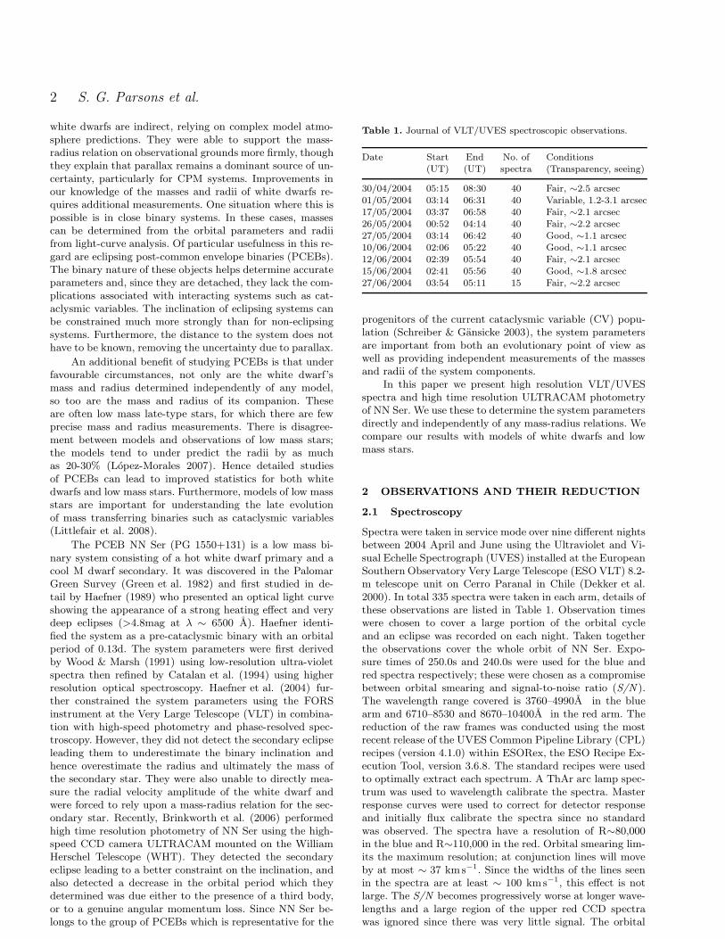
Precice mass and radius values for both components of the pre-CV NN Ser 3

Figure 1. Averaged, normalised UVES blue arm spectrum withthe blaze removed. IS corresponds to interstellar absorption fea-tures. The discontinuity at ∼ 4150A and the emission-like featureat ∼ 4820A are most likely instrumental features or artifacts ofthe UVES reduction pipeline as they are seen in all 335 spectra.

phase of each spectrum was calculated using the ephemerisof Brinkworth et al. (2006).

The spectral features seen are similar to those reportedby Catalan et al. (1994) and Haefner et al. (2004): Balmerlines, which appear as either emission or absorption depend-ing upon the phase, HeI and CaII emission lines and HeII4686A in absorption. The Paschen series is also seen inemission in the far red. In addition, MgII 4481A emissionis seen as well as a number of fainter MgII emission linesbeyond 7800A . Weak FeI emission lines are seen through-out the spectrum and faint CI emission is seen beyond8300A (see Table 4 for a full list of identified emission lines).The strength of all the emission lines is phase-dependent,peaking at phase 0.5, when the heated face of the secondarystar is in full view, then disappearing around the primaryeclipse. Several sharp absorption features are observed notto move over the orbital period, these are interstellar ab-sorption features and include interstellar CaII absorption.

2.2 Blaze Removal

An echelle grating produces a spectrum that drops as onemoves away from the blaze peak, this is known as the blazefunction. After reduction a residual ripple pattern was visi-ble in the blue spectra corresponding to the blaze function.This was approximately removed by fitting with a sinusoidof the form

B(λ) = a0 + a1 sin(2πφ) + a2λ sin(2πφ) (1)

+ a3 cos(2πφ) + a4λ cos(2πφ).

The phase (φ) was calculated by identifying the centralwavelength of each echelle order. The line table producedusing the ESORex recipe uves cal wavecal provided this in-formation. Then using the relation

λn(O − n) = c, (2)

where c and O are constants and λn is the central wavelengthof order n, gives us the phase. We find values of O = 125 andc = 465700, which are similar for all the spectra. Thereforethe phase of the ripple is

φ = 125 −465700

λ.

Since the phase is now known, Equation 1 reduces to a sim-ple linear fit. Figure 1 is a normalised average of all theUVES blue arm spectra with the blaze removed. Since thisis only a simple fit some residual pattern does remain afterdivision by the blaze function but overall the effect is greatlyreduced.

2.3 Photometry

The data presented here were collected with the high speedCCD camera ULTRACAM (Dhillon et al. 2007), mountedas a visitor instrument on the 4.2m William Herschel Tele-scope (WHT) and on the VLT in June 2007. A total of tenobservations were made in 2002 and 2003, and these datawere supplemented with observations made at a rate of ∼ 1– 2 a year up until 2008. ULTRACAM is a triple beam cam-era and most of our observations were taken simultaneouslythrough the SDSS u’, g’ and i’ filters. In a number of in-stances an r’ filter was used in place of i’ ; this was mainlyfor scheduling reasons. Additionally, a z’ filter was used inplace of i’ for one night in 2003.

A complete log of the observations is given in Table 2.We windowed the CCD in order to achieve an exposure timeof 2 – 3s, which we varied to account for the conditions. Thedead time was ∼ 25ms.

All of these data were reduced using the ULTRACAMpipeline software. Debiassing, flatfielding and sky back-ground subtraction were performed in the standard way. Thesource flux was determined with aperture photometry usinga variable aperture, whereby the radius of the aperture isscaled according to the FWHM. Variations in observing con-ditions were accounted for by determining the flux relativeto a comparison star in the field of view. There were a num-ber of additional stars in the field which we used to checkthe stability of our comparison. For the flux calibration wedetermined atmospheric extinction coefficients in the u’, g’and r’ bands and subsequently determined the absolute fluxof our targets using observations of standard stars (fromSmith et al. 2002) taken in twilight. We use this calibra-tion for our determinations of the apparent magnitudes ofthe two sources, although we present all light curves in fluxunits determined using the conversion given in Smith et al.(2002). Using our absorption coefficients we extrapolate allfluxes to an airmass of 0. The systematic error introducedby our flux calibration is < 0.1 mag in all bands. For alldata we convert the MJD times to the barycentric dynami-cal timescale, corrected to the solar system barycentre.

A number of comparison stars were observed, their lo-cations are shown in Figure 2 and details of these stars aregiven in Table 3. Where possible we use comparison star Csince it is brighter. However, in 2002 only comparison starD was observed and in the 2007 VLT data, comparison starsC and B were saturated in g’ and i’. We therefore use starC for the comparison in the u’ and star A for the g’ and i’.

The light curves were corrected for extinction differ-

4 S. G. Parsons et al.

Table 2. ULTRACAM observations of NN Ser. The primary eclipse occurs at phase 1, 2 etc.

Date Filters Telescope UT UT Average Phase Conditionsstart end exp time (s) range (Transparency, seeing)

17/05/2002 u’g’r’ WHT 21:54:40 02:07:54 2.4 0.85–2.13 Good, ∼1.2 arcsec18/05/2002 u’g’r’ WHT 21:21:20 02:13:17 3.9 0.39–1.23 Variable, 1.2-2.4 arcsec19/05/2002 u’g’r’ WHT 23:58:22 00:50:52 2.0 0.93–1.10 Fair, ∼2 arcsec20/05/2002 u’g’r’ WHT 00:58:23 01:57:18 2.3 0.86–1.14 Fair, ∼2 arcsec19/05/2003 u’g’z’ WHT 22:25:33 01:02:25 6.7 0.47–1.12 Variable, 1.5-3 arcsec21/05/2003 u’g’i’ WHT 00:29:00 04:27:32 1.9 0.32–0.59 Excellent, ∼1 arcsec22/05/2003 u’g’i’ WHT 03:24:57 03:50:40 2.0 0.36–0.08 Excellent, <1 arcsec24/05/2003 u’g’i’ WHT 22:58:55 23:33:49 2.0 0.90–0.08 Good, ∼1.2 arcsec25/05/2003 u’g’i’ WHT 01:29:45 02:15:58 2.0 0.39–0.64 Excellent, ∼1 arcsec03/05/2004 u’g’i’ WHT 22:13:44 05:43:11 2.5 0.37–2.27 Variable, 1.2-3.2 arcsec04/05/2004 u’g’i’ WHT 23:18:46 23:56:59 2.5 0.91–0.61 Variable, 1.2-3 arcsec09/03/2006 u’g’r’ WHT 01:02:34 06:46:49 2.0 0.91–2.70 Variable, 1.2-3 arcsec10/03/2006 u’g’r’ WHT 05:01:13 05:50:14 2.0 0.85–1.11 Excellent, <1 arcsec09/06/2007 u’g’i’ VLT 04:59:25 05:46:18 0.9 0.40–0.61 Excellent, ∼1 arcsec16/06/2007 u’g’i’ VLT 03:57:48 04:54:39 2.0 0.86–1.15 Good, ∼1.2 arcsec17/06/2007 u’g’i’ VLT 01:50:16 02:38:09 1.0 0.86–1.11 Excellent, <1 arcsec07/08/2008 u’g’r’ WHT 23:41:29 00:22:46 2.8 0.87–1.07 Excellent, <1 arcsec

Table 3. Comparison star magnitudes and positional offsets fromNN Ser. There were no i’ band observations of star D. The mag-nitudes for the white dwarf in NN Ser are shown in Table 6.

Star u’ g’ r’ i’ RA off. Dec off.(arcsec) (arcsec)

A 17.0 15.6 15.8 15.0 -34.1 +2.2B 16.0 14.7 15.1 14.3 -46.4 +106.7C 14.6 13.4 13.7 12.8 -114.5 +103.7D 16.7 14.6 13.7 – -22.2 -94.1

ences by using the comparison star observations. A first-order polynomial was fit to the comparison star photometryin order to determine the comparison star’s colours (mag-nitudes listed in Table 3). The colour of the white dwarf inNN Ser was calculated by fitting a zeroth-order polynomialto the flat regions around the primary eclipse with a cor-rection made in the r’ and i’ bands for the secondary starscontribution (the contribution of the secondary star in theu’ and g’ bands around the primary eclipse is negligible).The colour dependant difference in extinction coefficients forthe comparison star and NN Ser were then calculated froma theoretical extinction vs. colour plot1. The additional ex-tinction correction for NN Ser for each night is then

101

2.5(kN−kC )X , (3)

where kN is the extinction coefficient for NN Ser, kC is theextinction coefficient for the comparison and X is the air-mass. The value of kN −kC for each band was similar for allthe comparisons used. In the u’ filter kN − kC ∼ 0.03, forthe g’ band kN −kC ∼ 0.02, for the r’ band kN −kC ∼ 0.002and for the i’ band kN − kC ∼ 0.0005.

The flux-calibrated, extinction-corrected light curvesfor each filter were phase binned using the ephemeris ofBrinkworth et al. (2006). Data within each phase bin were

1 theoretical extinction vs. colour plots for ULTRACAM areavailable at http://garagos.net/dev/ultracam/filters

Figure 2. Digital Sky Survey finding chart (POSS II, blue) forNN Ser. Comparison stars are marked.

averaged using inverse variance weights whereby data withsmaller errors are given larger weightings. Smaller bins wereused around both the eclipses. The result of this is a set ofhigh signal-to-noise light curves for NN Ser (one for eachfilter).

2.4 Flux Calibration

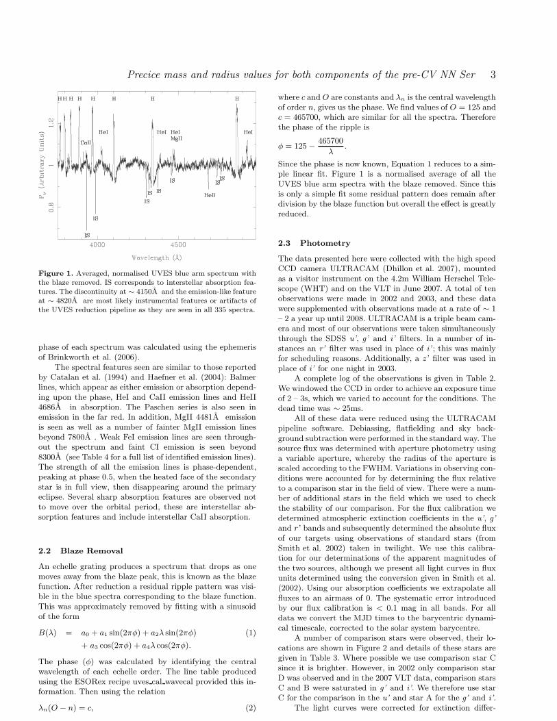
The ULTRACAM photometry was used to flux calibrateeach of the UVES spectra. Figure 3 shows the average spec-tra from each of the detectors (the UVES blue CCD spec-tra cover 3760–4990A , the lower red CCD spectra coverthe range 6710–8530 and the upper red CCD spectra cover

Precice mass and radius values for both components of the pre-CV NN Ser 5

Figure 3. Averaged spectra from the blue, lower and upper red CCD chips with ULTRACAM filter response curves. The spectra werenot telluric corrected. The dotted line is the filter profile based on the g’ filter used to flux calibrate the UVES blue CCD spectra sincethe g’ filter doesn’t cover the same spectra range.

Figure 4. Sine curve fit for the HeII 4686A absorption line fittedwith a straight line and a Gaussian. The measured radial velocityamplitude for the primary is 62.3 ± 1.9 km s−1.

8670–10400A ) along with ULTRACAM response curves foreach filter. A simple model was fitted to the ULTRACAM g’and i’ light curves (see Section 4.1 for details of the modelfitting). The aim of this model was to reproduce the lightcurve as closely as possible. The model was then used topredict the flux at the times of each of the UVES observa-tions (NN Ser shows no stochastic variations or flaring de-spite the rapidly rotating secondary star). Since the i’ filter

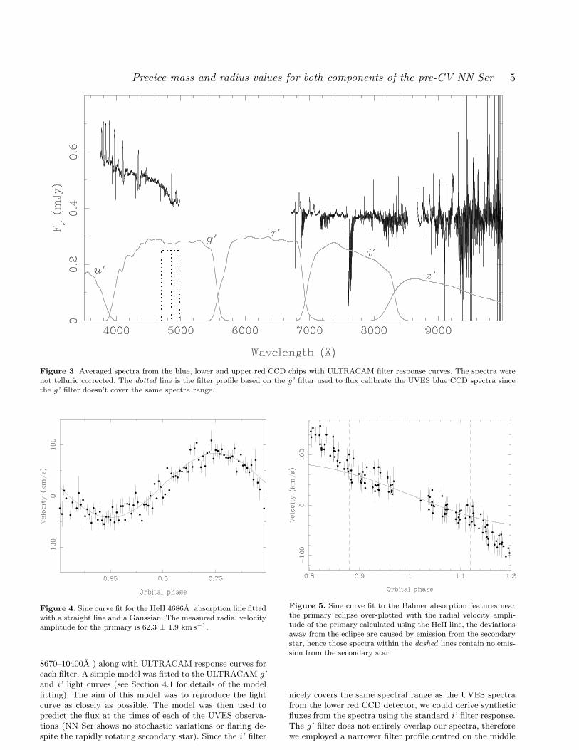
Figure 5. Sine curve fit to the Balmer absorption features nearthe primary eclipse over-plotted with the radial velocity ampli-tude of the primary calculated using the HeII line, the deviationsaway from the eclipse are caused by emission from the secondarystar, hence those spectra within the dashed lines contain no emis-sion from the secondary star.

nicely covers the same spectral range as the UVES spectrafrom the lower red CCD detector, we could derive syntheticfluxes from the spectra using the standard i’ filter response.The g’ filter does not entirely overlap our spectra, thereforewe employed a narrower filter profile centred on the middle

6 S. G. Parsons et al.

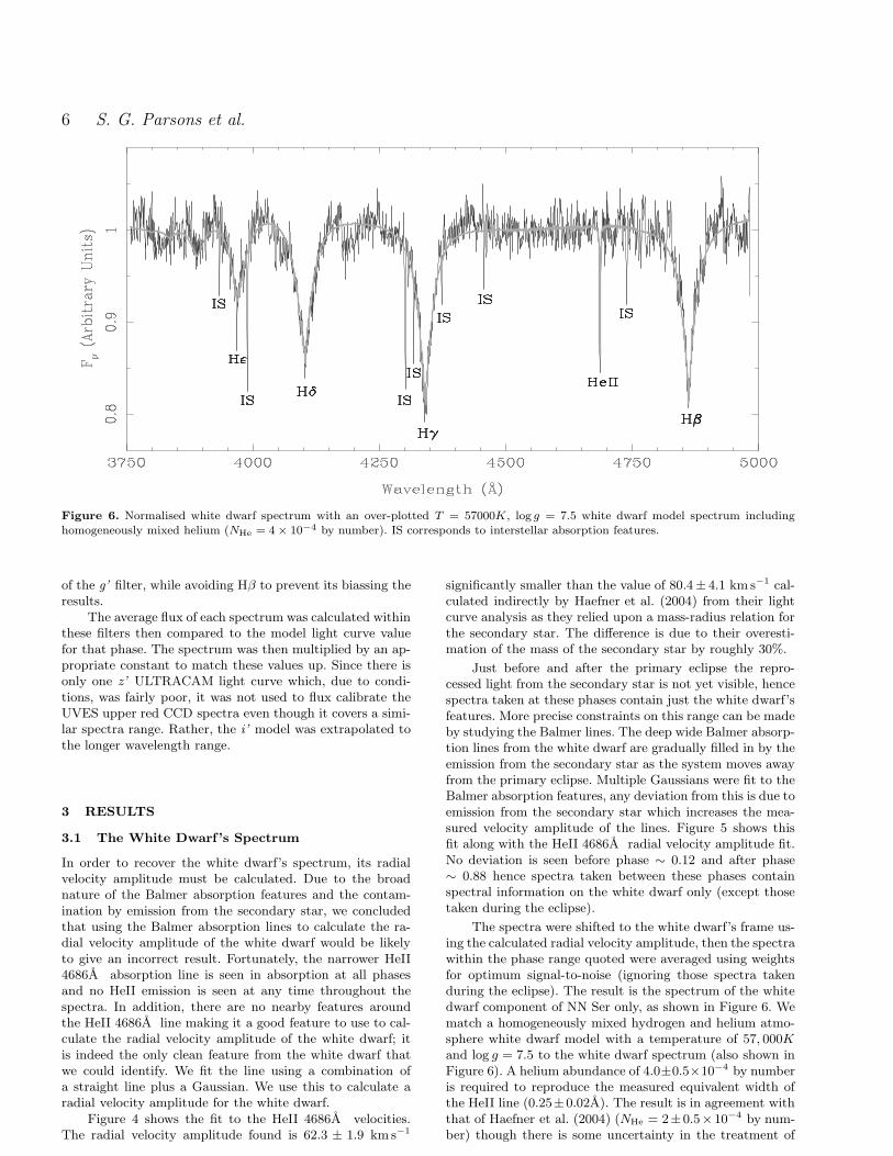
Figure 6. Normalised white dwarf spectrum with an over-plotted T = 57000K, log g = 7.5 white dwarf model spectrum includinghomogeneously mixed helium (NHe = 4 × 10−4 by number). IS corresponds to interstellar absorption features.

of the g’ filter, while avoiding Hβ to prevent its biassing theresults.

The average flux of each spectrum was calculated withinthese filters then compared to the model light curve valuefor that phase. The spectrum was then multiplied by an ap-propriate constant to match these values up. Since there isonly one z’ ULTRACAM light curve which, due to condi-tions, was fairly poor, it was not used to flux calibrate theUVES upper red CCD spectra even though it covers a simi-lar spectra range. Rather, the i’ model was extrapolated tothe longer wavelength range.

3 RESULTS

3.1 The White Dwarf’s Spectrum

In order to recover the white dwarf’s spectrum, its radialvelocity amplitude must be calculated. Due to the broadnature of the Balmer absorption features and the contam-ination by emission from the secondary star, we concludedthat using the Balmer absorption lines to calculate the ra-dial velocity amplitude of the white dwarf would be likelyto give an incorrect result. Fortunately, the narrower HeII4686A absorption line is seen in absorption at all phasesand no HeII emission is seen at any time throughout thespectra. In addition, there are no nearby features aroundthe HeII 4686A line making it a good feature to use to cal-culate the radial velocity amplitude of the white dwarf; itis indeed the only clean feature from the white dwarf thatwe could identify. We fit the line using a combination ofa straight line plus a Gaussian. We use this to calculate aradial velocity amplitude for the white dwarf.

Figure 4 shows the fit to the HeII 4686A velocities.The radial velocity amplitude found is 62.3 ± 1.9 km s−1

significantly smaller than the value of 80.4± 4.1 km s−1 cal-culated indirectly by Haefner et al. (2004) from their lightcurve analysis as they relied upon a mass-radius relation forthe secondary star. The difference is due to their overesti-mation of the mass of the secondary star by roughly 30%.

Just before and after the primary eclipse the repro-cessed light from the secondary star is not yet visible, hencespectra taken at these phases contain just the white dwarf’sfeatures. More precise constraints on this range can be madeby studying the Balmer lines. The deep wide Balmer absorp-tion lines from the white dwarf are gradually filled in by theemission from the secondary star as the system moves awayfrom the primary eclipse. Multiple Gaussians were fit to theBalmer absorption features, any deviation from this is due toemission from the secondary star which increases the mea-sured velocity amplitude of the lines. Figure 5 shows thisfit along with the HeII 4686A radial velocity amplitude fit.No deviation is seen before phase ∼ 0.12 and after phase∼ 0.88 hence spectra taken between these phases containspectral information on the white dwarf only (except thosetaken during the eclipse).

The spectra were shifted to the white dwarf’s frame us-ing the calculated radial velocity amplitude, then the spectrawithin the phase range quoted were averaged using weightsfor optimum signal-to-noise (ignoring those spectra takenduring the eclipse). The result is the spectrum of the whitedwarf component of NN Ser only, as shown in Figure 6. Wematch a homogeneously mixed hydrogen and helium atmo-sphere white dwarf model with a temperature of 57, 000Kand log g = 7.5 to the white dwarf spectrum (also shown inFigure 6). A helium abundance of 4.0±0.5×10−4 by numberis required to reproduce the measured equivalent width ofthe HeII line (0.25±0.02A). The result is in agreement withthat of Haefner et al. (2004) (NHe = 2±0.5×10−4 by num-ber) though there is some uncertainty in the treatment of

Precice mass and radius values for both components of the pre-CV NN Ser 7

Figure 7. Trailed spectra of various lines. The white dwarf component has been subtracted. White represents a value of 0.0 in alltrails. For the Balmer lines and the Paschen line, black represents a value of 2.0, for the other lines, black represents a value of 1.0. Thesubtraction of the white dwarf component creates a peak on the CaII trail due to the presence of interstellar absorption.

Figure 8. Sine curve fits for the Balmer lines (left), the three strongest He I lines (centre), and the MgII 4481A line (right). The lineswere fit using a straight line and a Gaussian. The MgII 4481A line becomes too faint before phase 0.15 and after phase 0.85 to fit.

Stark broadening in the code we used to calculate the model(TLUSTY, Hubeny 1988, Hubeny & Lanz 1995). The whitedwarf spectrum shows only Balmer and HeII 4686A absorp-tion features (the other sharp absorption features through-out the spectrum are interstellar absorption lines), no ab-sorption lines are seen in the red spectra. This confirmsprevious results that the classification of the white dwarfis of type DAO1 according to the classification scheme ofSion et al. (1983).

3.2 Secondary Star’s Spectrum

The most striking features of the UVES spectra are the emis-sion lines arising from the heated face of the secondary star,the most prominent of which are the Balmer lines. Figure 7

shows trailed spectra of several lines visible across the spec-tral range covered. The white dwarf component has beensubtracted which creates a peak on the CaII trail that ap-pears to move in anti-phase with the secondary, due to in-terstellar absorption. The top row shows three Balmer lines(Hδ,Hγ and Hβ) which clearly show reversed cores, becom-ing more prominent at increasing wavelength. Interestingly,the same effect is not visible in the Paschen series. Largebroadening is obvious in the Hydrogen lines.

Radial velocities can be measured from these lines us-ing the same multiple or single Gaussian plus polynomialapproximations used to fit the white dwarf features. How-ever, the measured radial velocity amplitude will be that ofthe emitting region on the face of the secondary star hencethe radial velocity amplitude of the centre of mass of the

8 S. G. Parsons et al.

secondary star will be larger than that measured from theselines (see Section 4.4). The white dwarf component shown inFigure 6 was subtracted from each spectrum and the emis-sion lines fitted. Due to the presence of interstellar absorp-tion features, the subtraction of the white dwarf componentcreates peaks in the spectra since they show no phase vari-ation. Figure 8 shows the fit to several lines: all the Balmerlines fitted simultaneously (H11 to Hβ), several HeI linesfitted simultaneously and a fit to the MgII 4481A line. Allthe lines show a similar deviation from a sinusoidal shape atsmall and large phases (. 0.25 and & 0.75). This is becauseof the non-uniform distribution of flux over the secondarystar. The radial velocity amplitude was calculated using onlythe points between these phases. The measured radial veloc-ity amplitude varies for each line, the Balmer lines showing alarger radial velocity amplitude than most of the other lines.In addition, the radial velocity amplitude of the Balmer linesdecreases towards the higher energy states. We believe thatthe spread in measured values is related to the optical depthfor each line; this is discussed in Section 4.4.

The Balmer, HeI and MgII lines from the UVES bluespectra were fitted with a polynomial and Gaussian. Fur-thermore, several HeI lines in the red spectra were fit aswell as the Paschen lines (P12 to Pǫ). Although several FeIlines are seen, they are too faint to calculate the radial ve-locity amplitude of the secondary star reliably. Nonetheless,they do show the same phase dependant variations as all theother emission lines.

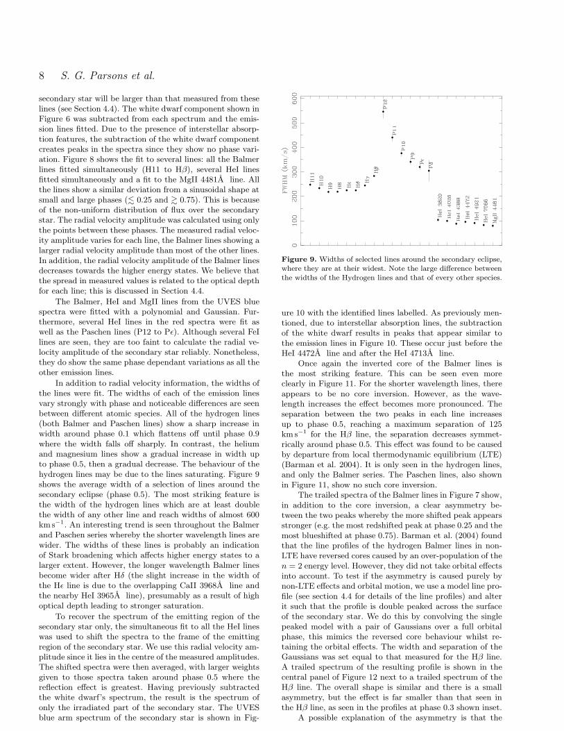
In addition to radial velocity information, the widths ofthe lines were fit. The widths of each of the emission linesvary strongly with phase and noticeable differences are seenbetween different atomic species. All of the hydrogen lines(both Balmer and Paschen lines) show a sharp increase inwidth around phase 0.1 which flattens off until phase 0.9where the width falls off sharply. In contrast, the heliumand magnesium lines show a gradual increase in width upto phase 0.5, then a gradual decrease. The behaviour of thehydrogen lines may be due to the lines saturating. Figure 9shows the average width of a selection of lines around thesecondary eclipse (phase 0.5). The most striking feature isthe width of the hydrogen lines which are at least doublethe width of any other line and reach widths of almost 600kms−1. An interesting trend is seen throughout the Balmerand Paschen series whereby the shorter wavelength lines arewider. The widths of these lines is probably an indicationof Stark broadening which affects higher energy states to alarger extent. However, the longer wavelength Balmer linesbecome wider after Hδ (the slight increase in the width ofthe Hǫ line is due to the overlapping CaII 3968A line andthe nearby HeI 3965A line), presumably as a result of highoptical depth leading to stronger saturation.

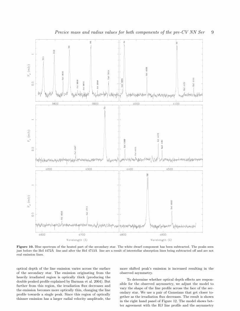
To recover the spectrum of the emitting region of thesecondary star only, the simultaneous fit to all the HeI lineswas used to shift the spectra to the frame of the emittingregion of the secondary star. We use this radial velocity am-plitude since it lies in the centre of the measured amplitudes.The shifted spectra were then averaged, with larger weightsgiven to those spectra taken around phase 0.5 where thereflection effect is greatest. Having previously subtractedthe white dwarf’s spectrum, the result is the spectrum ofonly the irradiated part of the secondary star. The UVESblue arm spectrum of the secondary star is shown in Fig-

Figure 9. Widths of selected lines around the secondary eclipse,where they are at their widest. Note the large difference betweenthe widths of the Hydrogen lines and that of every other species.

ure 10 with the identified lines labelled. As previously men-tioned, due to interstellar absorption lines, the subtractionof the white dwarf results in peaks that appear similar tothe emission lines in Figure 10. These occur just before theHeI 4472A line and after the HeI 4713A line.

Once again the inverted core of the Balmer lines isthe most striking feature. This can be seen even moreclearly in Figure 11. For the shorter wavelength lines, thereappears to be no core inversion. However, as the wave-length increases the effect becomes more pronounced. Theseparation between the two peaks in each line increasesup to phase 0.5, reaching a maximum separation of 125kms−1 for the Hβ line, the separation decreases symmet-rically around phase 0.5. This effect was found to be causedby departure from local thermodynamic equilibrium (LTE)(Barman et al. 2004). It is only seen in the hydrogen lines,and only the Balmer series. The Paschen lines, also shownin Figure 11, show no such core inversion.

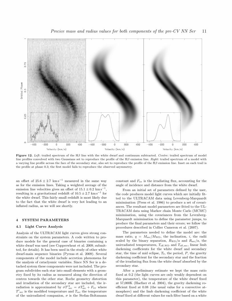
The trailed spectra of the Balmer lines in Figure 7 show,in addition to the core inversion, a clear asymmetry be-tween the two peaks whereby the more shifted peak appearsstronger (e.g. the most redshifted peak at phase 0.25 and themost blueshifted at phase 0.75). Barman et al. (2004) foundthat the line profiles of the hydrogen Balmer lines in non-LTE have reversed cores caused by an over-population of then = 2 energy level. However, they did not take orbital effectsinto account. To test if the asymmetry is caused purely bynon-LTE effects and orbital motion, we use a model line pro-file (see section 4.4 for details of the line profiles) and alterit such that the profile is double peaked across the surfaceof the secondary star. We do this by convolving the singlepeaked model with a pair of Gaussians over a full orbitalphase, this mimics the reversed core behaviour whilst re-taining the orbital effects. The width and separation of theGaussians was set equal to that measured for the Hβ line.A trailed spectrum of the resulting profile is shown in thecentral panel of Figure 12 next to a trailed spectrum of theHβ line. The overall shape is similar and there is a smallasymmetry, but the effect is far smaller than that seen inthe Hβ line, as seen in the profiles at phase 0.3 shown inset.

A possible explanation of the asymmetry is that the

Precice mass and radius values for both components of the pre-CV NN Ser 9

Figure 10. Blue spectrum of the heated part of the secondary star. The white dwarf component has been subtracted. The peaks seenjust before the HeI 4472A line and after the HeI 4713A line are a result of interstellar absorption lines being subtracted off and are notreal emission lines.

optical depth of the line emission varies across the surfaceof the secondary star. The emission originating from theheavily irradiated region is optically thick (producing thedouble peaked profile explained by Barman et al. 2004). Butfurther from this region, the irradiation flux decreases andthe emission becomes more optically thin, changing the lineprofile towards a single peak. Since this region of opticallythinner emission has a larger radial velocity amplitude, the

more shifted peak’s emission is increased resulting in theobserved asymmetry.

To determine whether optical depth effects are respon-sible for the observed asymmetry, we adjust the model tovary the shape of the line profile across the face of the sec-ondary star. We use a pair of Gaussians that get closer to-gether as the irradiation flux decreases. The result is shownin the right hand panel of Figure 12. The model shows bet-ter agreement with the Hβ line profile and the asymmetry

10 S. G. Parsons et al.

Figure 11. Left : Profiles of the Balmer lines. IS corresponds to interstellar absorption features. Right : Profiles of the Paschen lines. Thewhite dwarf component has been subtracted and the motion of the secondary star removed.

is visible. Hence it is necessary to allow for the variationin irradiation levels and hence the non-LTE core reversal inorder to model the line profiles in NN Ser.

Non-LTE effects have also been seen in other pre-cataclysmic variable systems such as HS 1857+5144(Aungwerojwit et al. 2007) where the Hβ and Hγ pro-files are clearly double-peaked, V664 Cas and EC 11575–1845 (Exter et al. 2005) both show Stark broadened Balmerline profiles with absorption components. Likewise, double-peaked Balmer line profiles were observed in HS 1136+6646(Sing et al. 2004) and Feige 24 (Vennes & Thorstensen1994); GD 448 (Maxted et al. 1998) also shows an asym-metry between the two peaks of the core-inverted Balmerlines. Since NN Ser is the only system observed with echelleresolution it shows this effect more clearly than any othersystem.

The secondary star’s spectrum contains a large num-ber of emission lines throughout. Each line was identifiedusing rest wavelengths obtained from the National Insti-

tute of Standards and Technology1 (NIST) atomic spectradatabase. The velocity offset (difference between the restand measured wavelength) and FWHM of each line wereobtained by fitting with a straight line and a Gaussian. Theline flux and equivalent width (EW) were also measured.Table 4 contains a complete list of all the lines identified.In addition to the already known hydrogen, helium and cal-cium lines, there are a number of MgII lines throughout thespectra as well as FeI lines in the blue spectra and CI linesin the red spectra. The EW of the Balmer lines increasesmonotonically from H11 to Hβ but the core inversion causesthe line flux to level off after the Hǫ line. In addition to thePaschen P12 to Pδ lines, half of the P13 line is seen (cut offby the spectral window used in the UVES upper red chip).

The offsets for each line measured in Table 4 combinedwith the measured offset of the HeII absorption line fromthe white dwarf, give a measurement of the gravitationalredshift of the white dwarf. The HeII absorption line has

1 http://physics.nist.gov/PhysRefData/ASD/lines form.html

Precice mass and radius values for both components of the pre-CV NN Ser 11

Figure 12. Left : trailed spectrum of the Hβ line with the white dwarf and continuum subtracted. Centre: trailed spectrum of modelline profiles convolved with two Gaussians set to reproduce the profile of the Hβ emission line. Right : trailed spectrum of a model witha varying line profile across the face of the secondary star, also set to reproduce the profile of the Hβ emission line. Inset on each trail isthe profile at phase 0.3; the first model fails to reproduce the observed asymmetry.

an offset of 25.6 ± 2.7 km s−1 measured in the same wayas for the emission lines. Taking a weighted average of theemission line velocities gives an offset of 15.1 ± 0.2 kms−1,resulting in a gravitational redshift of 10.5 ± 2.7 kms−1 forthe white dwarf. This fairly small redshift is most likely dueto the fact that the white dwarf is very hot leading to aninflated radius, as we will see shortly.

4 SYSTEM PARAMETERS

4.1 Light Curve Analysis

Analysis of the ULTRACAM light curves gives strong con-straints on the system parameters. A code written to pro-duce models for the general case of binaries containing awhite dwarf was used (see Copperwheat et al. 2009, submit-ted, for details). It has been used in the study of other whitedwarf-main sequence binaries (Pyrzas et al. 2009). Severalcomponents of the model include accretion phenomena forthe analysis of cataclysmic variables. Since NN Ser is a de-tached system these components were not included. The pro-gram subdivides each star into small elements with a geom-etry fixed by its radius as measured along the direction ofcentres towards the other star. Roche geometry distortionand irradiation of the secondary star are included, the ir-radiation is approximated by σT ′4

sec = σT 4sec + Firr where

T ′

sec is the modified temperature and Tsec the temperatureof the unirradiated companion, σ is the Stefan-Boltzmann

constant and Firr is the irradiating flux, accounting for theangle of incidence and distance from the white dwarf.

From an initial set of parameters defined by the user,the code produces model light curves which are initially fit-ted to the ULTRACAM data using Levenberg-Marquardtminimisation (Press et al. 1986) to produce a set of covari-ances. The resultant model parameters are fitted to the UL-TRACAM data using Markov chain Monte Carlo (MCMC)minimisation, using the covariances from the Levenberg-Marquardt minimisation to define the parameter jumps, toproduce the final parameters and their errors; we follow theprocedures described in Collier Cameron et al. (2007).

The parameters needed to define the model are: themass ratio, q = Msec/MWD, the inclination, i, the radiiscaled by the binary separation, RWD/a and Rsec/a, theunirradiated temperatures, Teff,WD and Teff,sec, linear limbdarkening coefficients for the white dwarf and secondarystar, the time of mid eclipse, T0, the period, P , the gravitydarkening coefficient for the secondary star and the fractionof the irradiating flux from the white dwarf absorbed by thesecondary star.

After a preliminary estimate we kept the mass ratiofixed at 0.2 (the light curves are only weakly dependent onthis parameter), the temperature of the white dwarf fixedat 57,000K (Haefner et al. 2004), the gravity darkening co-efficient fixed at 0.08 (the usual value for a convective at-mosphere) and the limb darkening coefficient of the whitedwarf fixed at different values for each filter based on a white

12 S. G. Parsons et al.

Table 4. Identified emission lines in the UVES spectra. Each line was fitted with a Gaussian to determinethe velocity and FWHM.

Line ID Velocity FWHM Line Flux (10−15 Equivalent comment(km s−1) (km s−1) ergs cm−2s−1A−1) Width (A)

H11 3770.634 16.4±1.5 250.7±4.1 3.10(4) 4.36(5) -H10 3797.910 12.6±1.1 233.9±2.9 3.46(4) 4.74(5) -HeI 3819.761 12.4±1.8 107.4±4.5 0.46(2) 0.69(3) -H9 3835.397 13.5±0.9 223.1±2.4 4.32(4) 6.30(6) -FeI 3856.327 11.0±3.7 63.2±9.9 0.12(1) 0.20(2) -FeI 3871.749 14.7±2.8 50.0±7.0 0.11(2) 0.20(3) -H8 3889.055 14.6±0.7 223.1±1.8 4.46(3) 6.51(4) -FeI 3906.479 10.1±3.6 68.2±8.8 0.22(2) 0.41(4) -CaII 3933.663 -2.9±1.4 106.8±3.7 0.64(2) 1.06(3) Interstellar absorption presentHeI 3964.727 12.2±3.2 85.7±8.0 0.30(2) 0.55(3) Close to the Hǫ lineHǫ 3970.074 4.6±0.7 249.4±2.0 5.44(3) 9.59(6) -HeI 4026.189 14.3±1.0 96.3±2.8 0.71(2) 1.28(3) -Hδ 4101.735 17.1±0.6 231.0±1.5 4.72(3) 8.57(5) -HeI 4120.824 10.3±4.4 73.9±9.8 0.12(1) 0.24(2) -HeI 4143.759 15.6±2.5 85.2±6.4 0.29(1) 0.59(3) -FeI 4266.964 12.8±4.5 97.9±10.5 0.22(2) 0.49(3) -Hγ 4340.465 14.5±0.6 255.9±1.5 4.74(2) 9.40(4) -HeI 4387.928 18.1±1.4 80.7±3.6 0.34(1) 0.74(2) -FeI 4415.122 15.5±4.4 66.4±11.1 0.18(1) 0.42(2) -HeI 4471.681 14.5±1.0 86.3±2.5 0.54(2) 1.15(2) -MgII 4481.327 16.9±1.3 89.5±3.5 0.33(1) 0.74(2) -FeI 4649.820 18.9±4.6 80.7±8.8 0.13(1) 0.30(2) -HeI 4713.146 14.7±1.4 76.6±3.7 0.12(1) 0.57(2) -Hβ 4861.327 14.7±0.4 262.0±1.3 4.26(2) 10.34(4) -HeI 4921.929 16.4±1.0 81.7±2.5 0.39(1) 1.05(2) -HeI 7065.709 15.4±0.4 78.4±1.1 0.27(3) 1.17(1) -HeI 7281.349 16.0±0.7 67.3±2.0 0.13(3) 0.64(1) -MgII 7877.051 12.6±3.1 37.1±7.8 0.12(3) 0.23(2) -MgII 7896.368 12.9±2.2 54.8±5.7 0.15(4) 0.30(2) -CI 8335.15 9.9±4.1 44.2±6.6 0.11(4) 0.20(3) -

CaII 8498.02 14.4±2.7 99.8±8.3 0.14(5) 0.90(3) -P12 8750.473 16.6±5.3 402.4±16.8 1.15(2) 5.49(1) Half of P13 line seen as wellP11 8862.784 16.5±2.7 376.2±8.0 1.68(2) 8.16(9) -CaII 8927.36 18.0±3.6 58.3±9.5 0.13(1) 0.65(5) -P10 9014.911 13.1±2.7 280.4±8.1 1.97(2) 10.27(9) -CI 9061.43 12.1±4.6 35.6±7.7 0.12(3) 0.28(4) -MgII 9218.248 16.2±2.6 48.9±7.6 0.12(6) 0.51(4) Close to the P9 lineP9 9229.015 15.1±1.3 316.5±3.6 2.42(2) 11.47(8) -MgII 9244.266 16.0±2.5 44.6±6.4 0.14(3) 0.40(3) -CI 9405.73 10.7±5.1 46.0±8.0 0.15(1) 0.87(7) -Pǫ 9545.972 16.4±2.3 332.3±6.4 3.39(4) 19.58(7) -Pδ 10049.374 18.4±7.4 253.4±22.2 2.7(1) 18.0(7) Very noisy in the far red

dwarf with Teff = 57, 000K and log g = 7.46 using ULTRA-CAM u’g’r’i’z’ filters (Gansicke et al. 1995). The log g wasobtained from an initial MCMC minimisation of the g’ lightcurve with the limb darkening coefficient of the white dwarffixed at a value of 0.2 (the log g determined from this isvery similar to the final value determined later). All otherparameters were optimised in the MCMC minimisation. Theinitial values for the inclination, radii and the temperatureof the secondary star were taken from Haefner et al. (2004),the limb darkening coefficient for the secondary star was ini-tially set to zero and the fraction of the irradiating flux fromthe white dwarf absorbed by the secondary star was initiallyset to 0.5 (note that the intrinsic flux of the secondary staris negligible).

Since phase-binned light curves were used, T0 was set tozero but allowed to change while the period was kept fixed at

1. The primary and secondary eclipses are the most sensitiveregions to the inclination and scaled radii. Hence, in orderto determine the most accurate inclination and radii, thedata around the two eclipses were given increased weightingin the fit (points with phases between 0.45 and 0.55 and be-tween 0.95 and 0.05 were given twice the weighting of otherpoints). We obtained z’ photometry for only one night andit was of fairly poor quality hence no model was fitted toit. The best fit parameters and their statistical errors aredisplayed in Table 5 along with the linear limb darkeningcoefficients used for the white dwarf. Figure 13 shows thefits to various light curves at different phases. For the sec-ondary eclipse light curves, the same model is over-plottedbut with the secondary eclipse turned off, demonstrating thehigh inclination of this system. The average χ2, per degreeof freedom, for the fits was 1.7 for the g’, r’ and i’ light

Precice mass and radius values for both components of the pre-CV NN Ser 13

Table 5. Best fit parameters from Markov chain Monte Carlo minimisation for each ULTRACAM light curve. Lin limb is the linear limbdarkening coefficient for the white dwarf which was kept fixed, the values quoted are for a model white dwarf of temperature 57,000Kand log g = 7.46. Absorb is the fraction of the irradiating flux from the white dwarf absorbed by the secondary star.

Parameter u’ g’ r’ i’

Inclination 89.18 ± 0.27 89.67 ± 0.05 89.31 ± 0.21 89.59 ± 0.27RWD/a 0.02262 ± 0.00014 0.02264 ± 0.00002 0.02271 ± 0.00010 0.02257 ± 0.00010Rsec/a 0.1660 ± 0.0011 0.1652 ± 0.0001 0.1657 ± 0.0007 0.1654 ± 0.0003Tsec 3962 ± 32 3125 ± 10 3108 ± 11 3269 ± 7Lin limbWD 0.125 0.096 0.074 0.060Lin limbsec −1.44 ± 0.13 −0.48 ± 0.03 −0.26 ± 0.02 −0.06 ± 0.03Absorb 0.899 ± 0.001 0.472 ± 0.001 0.604 ± 0.006 0.651 ± 0.005

Figure 13. Model fits to the ULTRACAM light curves with residuals shown below. Top: Full orbital phase. Centre: Around the primaryeclipse. Bottom: Around the secondary eclipse. Finer binning was used around both the eclipses. The r’ light curves are slightly noisieraround the eclipses because there is no VLT photometry for that filter. The secondary eclipse light curves are also shown with a modelwith the secondary eclipse turned off. Points around the primary and secondary eclipses were given twice the weighting of other pointsresulting in some residual effects seen in the residuals.

14 S. G. Parsons et al.

curves and 2.1 for the u’ light curve. The MCMC chainsshowed no variation beyond that expected from statisticalvariance and the probability distributions are symmetricaland roughly Gaussian.

The errors in Table 5 were scaled to give a reducedχ2 = 1. The inclination was determined by taking a weightedaverage and is found to be 89.6◦

± 0.2◦. This inclination ismuch higher than the 84.6◦ determined by Haefner et al.(2004) but is consistent with the inferred inclination of∼ 88◦ from Brinkworth et al. (2006). The scaled radius ofthe white dwarf is RWD/a = 0.0226 ± 0.0001 and the scaledradius of the secondary star is Rsec/a = 0.165±0.001. Givenour black body assumption, Tsec does not represent the truetemperature of the secondary star, it is effectively just a scal-ing factor. An interesting trend is seen in the limb darken-ing coefficients for the secondary star, which are all negative(limb brightening), the amount of limb brightening decreaseswith increasing wavelength. This is presumably the result ofseeing to different depths at different wavelengths.

Although the ULTRACAM z’ photometry was of fairlypoor quality (owing to conditions), it was good enough tomeasure the magnitude of the secondary star during theprimary eclipse. A zeroth-order polynomial was fit to the r’,i’ and z’ filter light curves during the primary eclipse. Themeasured magnitudes were: r’= 21.8±0.1, i’= 20.4±0.1 andz’= 19.6±0.1, which gives colours of (r’-i’ )sec = 1.4±0.1 and(i’-z’ )sec = 0.8 ± 0.1 which corresponds to a spectral typeof M4 ± 0.5 (West et al. 2005). This is consistent with theresults of Haefner et al. (2004) who fitted the spectral fea-tures of the secondary star taken during the primary eclipseto determine a spectral type of M4.75 ± 0.25.

4.2 Heating of the Secondary Star

One can make an estimate of the heating effect by compar-ing the intrinsic luminosity of the secondary star to that re-ceived from the white dwarf. We use the mass-luminosity re-lation from Scalo et al. (2007) determined by fitting a poly-nomial to the luminosities and binary star masses compiledby Hillenbrand & White (2004) to determine the luminosityof the secondary star as 1.4×10−3 L⊙. The luminosity of thewhite dwarf was calculated using LWD = 4πR2σT 4. Usingthe radius derived in Section 4.4 and the temperature fromHaefner et al. (2004) gives the luminosity of the white dwarfas 4.2 L⊙. Using the scaled radius of the secondary star fromTable 5 translates to the secondary star being hit by over20 times its own luminosity. Despite this, the colours (hencespectral type) of the unirradiated side are in agreement withthe derived mass (Baraffe & Chabrier 1996) (see Section 4.4for the mass derivation) showing that this extreme heatingeffect on one hemisphere of the secondary star has no mea-surable effect on the unirradiated hemisphere.

4.3 Distance to NN Ser

Absolute magnitudes for the white dwarf in NN Ser werecalculated using a model from Holberg & Bergeron (2006)for a DA white dwarf of mass 0.527M⊙, log g = 7.5 anda temperature of 60,000K which most closely matched theparameters found for NN Ser. We give an uncertainty of±0.1 magnitudes for the absolute magnitudes based on the

Table 6. Distance measurements from each of the ULTRACAMlight curves. The absolute magnitudes for the white dwarf in NNSer were obtained from Holberg & Bergeron (2006) with an errorof ±0.1 magnitudes.

Filter Absolute Measured Extinction DistanceMagnitude Magnitude (mags) (pc)

u’ 7.264 15.992 ± 0.006 0.258 ± 0.258 494 ± 63g’ 7.740 16.427 ± 0.002 0.190 ± 0.190 501 ± 49r’ 8.279 16.931 ± 0.004 0.138 ± 0.138 505 ± 40i’ 8.666 17.309 ± 0.004 0.104 ± 0.104 510 ± 34z’ 9.025 17.71 ± 0.01 0.074 ± 0.074 527 ± 30

uncertainty in temperature from Haefner et al. (2004) andits effect on the models of Holberg & Bergeron (2006). Themagnitudes of the white dwarf in NN Ser were calculated byfitting a zeroth-order polynomial to the flat regions eitherside of the primary eclipse with a correction made for theflux of the secondary star. Using the reddening value of E(B-V)= 0.05 ± 0.05 from Wood & Marsh (1991) we correct theapparent magnitudes using the conversion of Schlegel et al.(1998). From these a distance was calculated for each ofthe ULTRACAM filters. Table 6 lists the distances calcu-lated in each of these filters. Using these values gives a dis-tance to NN Ser of 512± 43 pc consistent with the result ofHaefner et al. (2004) of 500 ± 35 pc.

The galactic latitude of NN Ser is 45.3◦ which, com-bined with the derived distance, gives NN Ser a galacticscale height of 364 ± 31 pc. The proper motion of NN Serwas retrieved from the US Naval Observatory (USNO) Im-age and Catalogue Archive. The archive values are µRA =−0.020 ± 0.003 and µDEC = −0.056 ± 0.004 arcsec / yr. Atthe derived distance this corresponds to a transverse velocityfor NN Ser of 160 ± 14 km s−1.

4.4 Ksec correction

The emission lines seen in the UVES spectra are the re-sult of reprocessed light from the surface of the secondarystar facing the white dwarf. Hence, their radial velocity am-plitude represents a lower limit to the true centre of massradial velocity amplitude. For accurate mass determinationsthe centre of mass radial velocity amplitude is required thuswe need to determine the deviation between the reprocessedlight centre and the centre of mass for the secondary star.We do this by computing model line profiles from the irra-diated face.

We use the inclination and radii determined from thelight curve model and account for Roche distortion of thesecondary star and the secondary eclipse. All other parame-ters are set to match the UVES spectra: the line profiles werecalculated for phases matching the UVES spectra phases, ex-posure lengths were set to the same as the UVES blue spec-tra exposures and sampled in velocity to match the spectra.The profiles are convolved with a Gaussian function, repre-senting the resolution of the spectrograph. In order to matchthe UVES spectroscopy as closely as possible, the resolutionof the spectrograph was calculated by looking at the arccalibration spectra. The intrinsic linewidth of these lines isassumed to be negligible hence the measured linewidth gives

Precice mass and radius values for both components of the pre-CV NN Ser 15

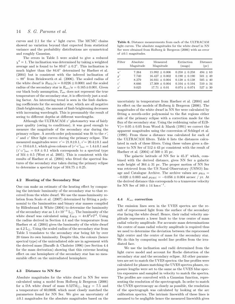
Figure 14. Light curves of various lines over-plotted with anoptically thick (narrower) and thin (wider) model with the samemeasured Ksec as the line. The model light curves are scaled tomatch the flux level of the lines around phase 0.5. The Hβ line isoptically thick, the MgII line is optically thin and the HeI line issomewhere between thick and thin.

an indication of the instrumental resolution, which we foundto be 5 km s−1 (FWHM) for the UVES blue chip.

As mentioned previously, the measured radial velocityamplitude varies for each line. We believe that this scatter isthe result of differences in optical depths of the lines, whichwill affect the angular distribution of line flux from any givenpoint on the star resulting in a range of observed radialvelocity amplitudes. Hence, the model is required to produceline profiles over a continuous range of optical depths (seeAppendix for details of the model).

The radiation from the secondary star is modelled asa slab of constant optical depth (τ0) and the source func-tion changes exponentially with depth, the factor that deter-mines how this changes is β (i.e. the source function changes

Table 7. Measured and corrected values of Ksec with the bestfit model line profiles parameters, for several lines in the UVESblue spectra.

Line τ0 β Ksec,meas Ksec,corr qkms−1 km s−1

HeI 3820 2 −0.75 252.2 ± 1.9 296.7 ± 1.9 0.210(6)HeI 4026 1 −3 257.7 ± 1.7 300.1 ± 1.7 0.208(6)HeI 4388 1 −10 249.9 ± 2.0 300.2 ± 2.0 0.208(6)HeI 4472 1 −1.5 263.1 ± 1.8 305.2 ± 1.8 0.204(6)HeI 4922 1 −0.5 255.6 ± 1.8 296.9 ± 1.8 0.210(6)Hβ 100 −1.5 271.1 ± 1.9 307.6 ± 1.9 0.203(6)Hγ 100 −1.5 265.1 ± 1.9 302.9 ± 1.9 0.206(6)Hδ 50 −1.5 265.0 ± 1.9 298.1 ± 1.9 0.209(6)Hǫ 5 −1.25 263.2 ± 1.9 304.4 ± 1.9 0.205(6)H8 5 −1 262.5 ± 1.9 303.2 ± 1.9 0.206(6)H9 2 −0.5 258.1 ± 1.9 297.4 ± 1.9 0.210(6)H10 2 −0.75 257.2 ± 2.1 299.9 ± 2.1 0.208(6)H11 1 −2 259.3 ± 2.1 301.2 ± 2.1 0.207(6)MgII 4481 0.005 −1.25 252.8 ± 1.8 298.7 ± 1.8 0.209(6)

with vertical optical depth (τ ) as eβτ ), this allows one tohave a continuous transition from optically thin to thick andto have limb darkening or brightening. We keep KWD fixedat the measured value of 62.3 kms−1, and just change Ksec.We measured the radial velocity amplitude of the resultingline profiles in the same way as for the emission lines in theUVES spectra. Initially, Ksec was set to give a measured ra-dial velocity amplitude of 252.8 km s−1 (the measured radialvelocity amplitude of the MgII 4482A line) and the valuesof the total vertical optical depth and source function ex-ponential factor were allowed to vary. The light curves pro-duced were fitted to the MgII 4481A line light curve usingleast squares fitting to determine the optimal values for τ0

and β. This was repeated for several lines in the UVES bluespectra adjusting Ksec to produce the measured radial veloc-ity amplitude for that line. Figure 14 shows the light curvefor three different lines over plotted with an optically thickand optically thin model. For the Hβ line, the emission isoptically thick, the MgII line is optically thin and the HeIline lies somewhere between these two extremes (the whitedwarf component was subtracted from all the light curves).Table 7 lists the best fit values for τ0 and β for each line andthe measured and corrected Ksec and q values.

The MgII 4481A line appears to be the closest to theoptically thin model. As such it probably provides the mostaccurate correction since, in the optically thin case, the an-gular distribution of the line flux from any given point onthe star is even, removing any dependence upon this. Evenso, all the corrected values are consistent to within a fewkms−1. The first few Balmer lines (Hβ to Hδ) are opticallythick but as the series progresses, the lines become moreoptically thin. There also appears to be a small increase inthe value of β throughout the series (with the exception ofH10 and H11). The helium lines appear to be somewherebetween optically thick and thin.

Figure 15 shows the measured values of Ksec for sev-eral lines from Gaussian fitting in the UVES blue spectraand their corrected values of Ksec. The spread in values isreduced and the corrected values give a radial velocity am-plitude for the secondary star of Ksec = 301 km s−1. Thestatistical uncertainty is 1 km s−1, however, we believe the

16 S. G. Parsons et al.

Figure 15. Bottom: Measured Ksec for several lines in the UVESblue spectra from Gaussian fitting and their corrected values(top). The CaII line is contaminated by interstellar absorptionwhich was fitted as an additional Gaussian component and wasnot corrected. The fit to all the Balmer lines simultaneously isthe point labelled ‘balmers’. The point labelled ‘HeI’s’ is a fit toall the visible HeI lines whilst the point labelled ‘single HeI’s’ isa fit to only the HeI lines which have a single component (i.e. theintensity is not shared by several lines).

error in the correction is dominated by systematic effectsfrom the model and fitting process, for which we estimatean error of 3 kms−1 for the radial velocity amplitude ofthe secondary star. Some simple considerations can give anidea of the largest possible error we might have made in cor-recting the K values. The distance from the centre of themass to the sub-stellar point in terms of velocity is given by(KWD + Ksec) Rsec/a = 60 kms−1; this is maximum possi-ble correction. A lower limit comes from assuming the emis-sion to be uniform over the irradiated face of the secondary.Then the centre of light is 0.42 of the way from the cen-tre of mass to the sub-stellar point (Wade & Horne 1988),leading to a lower limit on the correction of 24 kms−1. Thecorrections from our model range from 33 to 46 kms−1, inthe middle of these extremes.

From the corrected value and KWD = 62.3±1.9 km s−1

we determine the mass ratio as q = Msec/MWD = 0.207 ±

0.006. Using this, the mass of the white dwarf is then deter-mined using Kepler’s third law

PK3sec

2πG=

MWD sin3 i

(1 + q)2, (4)

using the period (P ) from Brinkworth et al. (2006). Thisgives a value of MWD = 0.535 ± 0.012 M⊙. The mass ratiothen gives the mass of the secondary star as Msec = 0.111±0.004 M⊙. Knowing the masses, the orbital separation isfound using

a3 =G(MWD + Msec)P

2

4π2, (5)

which gives a value of a = 0.934 ± 0.009 R⊙. Using thisgives the radii of the two stars as RWD = 0.0211 ± 0.0002R⊙ and Rsec = 0.154 ± 0.002 R⊙. The radius of the sec-ondary star in our model is measured from the centre of

Table 8. System parameters. (1) this paper; (2) Brinkworth et al.(2006); (3) Haefner et al. (2004). WD: white dwarf, Sec: sec-ondary star.

Parameter Value Ref.

Period (days) 0.13008017141(17) (2)Inclination 89.6 ± 0.2◦ (1)Binary separation 0.934 ± 0.009 R⊙ (1)Mass ratio 0.207 ± 0.006 (1)WD mass 0.535 ± 0.012 M⊙ (1)Sec mass 0.111 ± 0.004 M⊙ (1)WD radius 0.0211 ± 0.0002 R⊙ (1)Sec radius polar 0.147 ± 0.002 R⊙ (1)Sec radius sub-stellar 0.154 ± 0.002 R⊙ (1)Sec radius backside 0.153 ± 0.002 R⊙ (1)Sec radius side 0.149 ± 0.002 R⊙ (1)Sec radius volume-averaged 0.149 ± 0.002 R⊙ (1)WD log g 7.47 ± 0.01 (1)WD temperature 57000 ± 3000 K (3)KWD 62.3 ± 1.9 km s−1 (1)Ksec 301 ± 3 kms−1 (1)WD grav. redshift 10.5 ± 2.7 km s−1 (1)WD type DAO1 (3)Sec spectral type M4 ± 0.5 (1)Distance 512 ± 43 pc (1)WD hydrogen layer fractional mass 10−4 (1)

mass towards the white dwarf and hence is larger than theaverage radius of the secondary star. The radius as mea-sured towards the backside is Rsec,back = 0.153 R⊙, thepolar radius is Rsec,pol = 0.147 R⊙ and perpendicular tothese Rsec,side = 0.149 R⊙. The volume-averaged radius isRsec,av = 0.149 ± 0.002 R⊙.

The surface gravity of the white dwarf is given by

g =GMWD

RWD2

, (6)

which gives a value of log g = 7.47 ± 0.01.

5 DISCUSSION

Figure 16 shows the mass and radius of the white dwarf ofNN Ser in comparison with other white dwarfs whose massand radius have been measured independently of any mass-radius relation. The white dwarf of NN Ser has the largestmeasured radius of any white dwarf (not determined by amass-radius relation) placing it in a new area of this plot;it is also one of the most precisely measured. NN Ser is alsomuch hotter than the other white dwarfs in Figure 16, themean temperature of the other white dwarfs is ∼ 14, 200K.Also plotted are several mass-radius relations for pure hy-drogen atmosphere white dwarfs with different temperaturesand hydrogen layer thicknesses from Holberg & Bergeron(2006) and Benvenuto & Althaus (1999). The earlier workfrom Haefner et al. (2004) and the UVES spectrum of thewhite dwarf with a model white dwarf spectra over-plotted(Figure 6) strongly suggest a temperature for the whitedwarf of close to 60,000K (57000 ± 3000K). Assuming themodels in Figure 16 are correct, the white dwarf in NN Sershows excellent agreement with having a ‘thick’ hydrogenlayer of fractional mass MH/MWD = 10−4. This is consis-

Precice mass and radius values for both components of the pre-CV NN Ser 17

Figure 16. Mass-radius plot for white dwarfs measured inde-pendent of any mass-radius relations. Data from Provencal et al.(1998), Provencal et al. (2002) and Casewell et al. (2009) areplotted. The filled circles are visual binaries and the open cir-cles are common proper-motion systems. The solid lines corre-

spond to different carbon-oxygen core pure hydrogen atmospheremodels. The first number is the temperature, in thousands ofdegrees, the second number is the hydrogen layer thickness (i.e.lines labelled -4 have a thickness of MH/MWD = 10−4) fromHolberg & Bergeron (2006) and Benvenuto & Althaus (1999).The dashed line is the zero-temperature mass-radius relation ofEggleton from Verbunt & Rappaport (1988).

tent with the inflated radius of the white dwarf due to itshigh temperature.

Since visual binary systems and common proper-motionsystems still rely on model atmosphere calculations to de-termine radii, the white dwarf in NN Ser is one of thefirst to have its mass and radius measured independently.O’Brien et al. (2001) determine the mass and radius of bothcomponents of the eclipsing PCEB V471 Tau independentlyhowever, since they did not detect a secondary eclipse, theyhad to rely on less direct methods to determine the radiusof the secondary and the inclination. This demonstrates thevalue of eclipsing PCEBs for investigating the mass-radiusrelation for white dwarfs.

In addition, the mass and radius of the secondary starhave been determined independently of any mass-radius re-lation. Since this is a low mass star it helps improve thestatistics for these objects and our values are more precisethan the majority of comparable measurements. Figure 17shows the position of the secondary star in NN Ser (usingthe volume-averaged radius) in relation to other low massstars with masses and radii determined independently of anymass-radius relation (although the masses of the single starswere determined using mass-luminosity relations). For verylow mass stars (M . 0.3 M⊙) the current errors on massand radius measurements are so large that that one can ar-gue the data are consistent with the low-mass models. How-ever, the secondary star in NN Ser appears to be the firstobject with errors small enough to show an inconsistencywith the models. The measured radius is 10% larger thanpredicted by the model. However, irradiation increases theradius of the secondary star. For the measured radius of thesecondary star in NN Ser, the work of Ritter et al. (2000)

Figure 17. Mass-radius plot for low mass stars. Data fromLopez-Morales (2007) and Beatty et al. (2007). The filled circlesare secondaries in binaries, the open circles are low mass bina-ries and the crosses are single stars. The solid line represents thetheoretical isochrone model from Baraffe et al. (1998), for an ageof 0.4 Gyr, solar metalicity, and mixing length α = 1.0, the dot-ted line is the same but for an age of 4 Gyr. The position of thesecondary star in NN Ser is also shown if there were no irradia-tion effects. The masses of the single stars were determined usingmass-luminosity relations.

and Hameury & Ritter (1997) gives an inflation of 5.6%. Theun-irradiated radius is also shown in Figure 17 and is consis-tent with the models. Hence the secondary star in NN Sersupports the theoretical mass-radius relation for very lowmass stars. Potentially, an initial-final mass relation couldbe used to estimate the age of NN Ser, but since the systemhas passed through a common envelope phase its evolutionmay have been accelerated and the white dwarf may be lessmassive than a single white dwarf with the same progenitormass leading to an overestimated age. In addition, the massof the white dwarf in NN Ser is close to the mean whitedwarf mass and the initial-final mass relation is flat in thisregion. This means a large range of progenitor masses arepossible for the white dwarf and hence a large range in age,this means a reliable estimate of the age of NN Ser is notpossible. In any case, the position of the un-irradiated sec-ondary star is also consistent with a similarly large rangeof ages. The mass and radius of the secondary star supportthe argument of Brinkworth et al. (2006) that it is not ca-pable of generating enough energy to drive period changevia Applegate’s mechanism (Applegate 1992).

The system parameters determined for NN Ser are sum-marised in Table 8. Using the UVES spectra, the gravita-tional redshift of the white dwarf was found to be 10.5± 2.7kms−1. Using the measured mass and radius from Table 8gives a redshift of 16.1 kms−1, correcting for the redshiftof the secondary star (0.5 kms−1), the difference in trans-verse Doppler shifts (0.15 kms−1) and the potential at thesecondary star owing to the white dwarf (0.3 kms−1) givesa value of 15.2 ± 0.5 kms−1 which is consistent with themeasured value to ∼ 2 sigma, although in this case, the in-flated radius of the white dwarf weakens the constraints ofthe gravitational redshift.

18 S. G. Parsons et al.

6 CONCLUSIONS

We have measured precise masses and radii of the whitedwarf and M dwarf components of the post common en-velope binary NN Serpentis using UVES spectroscopy andULTRACAM photometry.

Using the HeII 4686A absorption line from the whitedwarf we determined the radial velocity amplitude of thewhite dwarf directly from the spectra. Using a number ofemission lines in the UVES spectra originating from theheated face of the secondary star, we were able to correctthe radial velocity amplitude of the secondary star from theheated face to the centre of mass of the secondary star itself.

From analysis of ULTRACAM light curves we deter-mine a system inclination of 89.6◦

± 0.2◦, higher than thevalue of 84.6◦

± 1.1◦ found by Haefner et al. (2004) which,along with our direct determination of KWD, leads to a lowermass ratio than previously derived. The radius of the whitedwarf is found to be RWD = 0.0211±0.0002 R⊙, larger thanin previous studies but, given its temperature, is consistentwith its derived mass of MWD = 0.535 ± 0.012 M⊙. Themass and radius of the white dwarf show excellent agree-ment with a hot carbon-oxygen core white dwarf with a‘thick’ hydrogen layer of fractional mass MH/MWD = 10−4.

The mass of the secondary star is found to be Msec =0.111 ± 0.004 M⊙ with a volume-averaged radius of Rsec =0.149 ± 0.002 R⊙, which is smaller than previously deter-mined. The radius of the secondary star is consistent withmodels if a ∼ 6% correction is made for the irradiation itreceives from the white dwarf.

The ULTRACAM photometry also provided colours forthe secondary star and thus a spectral type. This was con-sistent with the derived mass showing that, despite beingirradiated by over 20 times its own luminosity, there is verylittle backside heating, although infrared data are needed todetermine this more accurately. Finally, using model whitedwarf data we determine a distance to NN Ser of 512 ± 43pc, consistent with previous studies.

ACKNOWLEDGEMENTS

We thank the referee, M Burleigh, for his useful commentsand suggestions. TRM, CMC and BTG acknowledge sup-port from the Science and Technology Facilities Council(STFC) grant number ST/F002599/1. SPL acknowledgesthe support of an RCUK Fellowship. ULTRACAM, VSDand SPL are supported by STFC grants ST/G003092/1and PP/E001777/1. The results presented in this paper arebased on observations collected at the European SouthernObservatory (La Silla) under programme ID 073.D-0633 andwith the William Herschel Telescope operated on the islandof La Palma by the Isaac Newton Group in the SpanishObservatorio del Roque de los Muchachos of the Institu-tions de Astrofisica de Canarias. We used SIMBAD, main-tained by the Centre de Donnees astronomiques de Stras-bourg, and the National Aeronautics and Space Adminis-tration (NASA) Astrophysics Data System. This researchhas made use of the USNOFS Image and Catalogue Archiveoperated by the United States Naval Observatory, FlagstaffStation and the National Institute of Standards and Tech-nology (NIST) Atomic Spectra Database (version 3.1.5).

STScI is operated by the Association of Universities for Re-search in Astronomy inc.

REFERENCES

Applegate J. H., 1992, ApJ, 385, 621Aungwerojwit A., Gansicke B. T., Rodrıguez-Gil P., HagenH.-J., Giannakis O., Papadimitriou C., Allende Prieto C.,Engels D., 2007, A&A, 469, 297

Baraffe I., Chabrier G., 1996, ApJ, 461, L51+Baraffe I., Chabrier G., Allard F., Hauschildt P. H., 1998,A&A, 337, 403

Barman T. S., Hauschildt P. H., Allard F., 2004, ApJ, 614,338

Beatty T. G., Fernandez J. M., Latham D. W., Bakos G. A.,Kovacs G., Noyes R. W., Stefanik R. P., Torres G., EverettM. E., Hergenrother C. W., 2007, ApJ, 663, 573

Benvenuto O. G., Althaus L. G., 1999, MNRAS, 303, 30Brinkworth C. S., Marsh T. R., Dhillon V. S., Knigge C.,2006, MNRAS, 365, 287

Casewell S. L., Dobbie P. D., Napiwotzki R., BurleighM. R., Barstow M. A., Jameson R. F., 2009, MNRAS,395, 1795

Catalan M. S., Davey S. C., Sarna M. J., Connon-SmithR., Wood J. H., 1994, MNRAS, 269, 879

Collier Cameron A. et al., 2007, MNRAS, 380, 1230Copperwheat C. M., Marsh T. M., Dhillon V. S., LittlefairS. P., Hickman R., Gansicke B. T., Southworth J., 2009,MNRAS, 0, 0

Dekker H., D’Odorico S., Kaufer A., Delabre B., Kot-zlowski H., 2000, in Iye M., Moorwood A. F., eds, So-ciety of Photo-Optical Instrumentation Engineers (SPIE)Conference Series Vol. 4008 of Presented at the Societyof Photo-Optical Instrumentation Engineers (SPIE) Con-ference, Design, construction, and performance of UVES,the echelle spectrograph for the UT2 Kueyen Telescope atthe ESO Paranal Observatory. pp 534–545

Dhillon V. S., Marsh T. R., Stevenson M. J., AtkinsonD. C., Kerry P., Peacocke P. T., Vick A. J. A., BeardS. M., Ives D. J., Lunney D. W., McLay S. A., TierneyC. J., Kelly J., Littlefair S. P., Nicholson R., Pashley R.,Harlaftis E. T., O’Brien K., 2007, MNRAS, 378, 825

Exter K. M., Pollacco D. L., Maxted P. F. L., NapiwotzkiR., Bell S. A., 2005, MNRAS, 359, 315

Gansicke B. T., Beuermann K., de Martino D., 1995, A&A,303, 127

Green R. F., Ferguson D. H., Liebert J., Schmidt M., 1982,PASP, 94, 560

Haefner R., 1989, A&A, 213, L15Haefner R., Fiedler A., Butler K., Barwig H., 2004, A&A,428, 181

Hameury J.-M., Ritter H., 1997, A&AS, 123, 273Hillenbrand L. A., White R. J., 2004, ApJ, 604, 741Holberg J. B., Bergeron P., 2006, AJ, 132, 1221Hubeny I., 1988, Comput.,Phys.,Comm., 52, 103Hubeny I., Lanz T., 1995, ApJ, 439, 875Littlefair S. P., Dhillon V. S., Marsh T. R., Gansicke B. T.,Southworth J., Baraffe I., Watson C. A., Copperwheat C.,2008, MNRAS, 388, 1582

Lopez-Morales M., 2007, ApJ, 660, 732

Precice mass and radius values for both components of the pre-CV NN Ser 19

Maxted P. F. L., Marsh T. R., Moran C., Dhillon V. S.,Hilditch R. W., 1998, MNRAS, 300, 1225

O’Brien M. S., Bond H. E., Sion E. M., 2001, ApJ, 563,971

Press W. H., Flannery B. P., Teukolsky S. A., 1986, Numer-ical recipes. The art of scientific computing. Cambridge:University Press, 1986

Provencal J. L., Shipman H. L., Hog E., Thejll P., 1998,ApJ, 494, 759

Provencal J. L., Shipman H. L., Koester D., Wesemael F.,Bergeron P., 2002, ApJ, 568, 324

Pyrzas S., Gansicke B. T., Marsh T. R., Aungwerojwit A.,Rebassa-Mansergas A., Rodrıguez-Gil P., Southworth J.,Schreiber M. R., Nebot Gomez-Moran A., Koester D.,2009, MNRAS, 394, 978

Renzini A., Bragaglia A., Ferraro F. R., Gilmozzi R., Or-tolani S., Holberg J. B., Liebert J., Wesemael F., BohlinR. C., 1996, ApJ, 465, L23+

Ritter H., Zhang Z.-Y., Kolb U., 2000, A&A, 360, 969Scalo J., Kaltenegger L., Segura A. G., Fridlund M., RibasI., Kulikov Y. N., Grenfell J. L., Rauer H., Odert P.,Leitzinger M., Selsis F., Khodachenko M. L., Eiroa C.,Kasting J., Lammer H., 2007, Astrobiology, 7, 85

Schlegel D. J., Finkbeiner D. P., Davis M., 1998, ApJ, 500,525

Schmidt H., 1996, A&A, 311, 852Schreiber M. R., Gansicke B. T., 2003, A&A, 406, 305Sing D. K., Holberg J. B., Burleigh M. R., Good S. A.,Barstow M. A., Oswalt T. D., Howell S. B., BrinkworthC. S., Rudkin M., Johnston K., Rafferty S., 2004, AJ, 127,2936

Sion E. M., Greenstein J. L., Landstreet J. D., Liebert J.,Shipman H. L., Wegner G. A., 1983, ApJ, 269, 253

Smith J. A. et al., 2002, AJ, 123, 2121Vennes S., Thorstensen J. R., 1994, AJ, 108, 1881Verbunt F., Rappaport S., 1988, ApJ, 332, 193Wade R. A., Horne K., 1988, ApJ, 324, 411West A. A., Walkowicz L. M., Hawley S. L., 2005, PASP,117, 706

Wood J. H., Marsh T. R., 1991, ApJ, 381, 551Wood M. A., 1992, ApJ, 386, 539

APPENDIX A: MODELLING OF THE

IRRADIATION LINES

The radial velocity semi-amplitudes we measure for theemission lines in NN Ser reflect the distance from the cen-tre of mass of the binary of the irradiated face of the sec-ondary star. To obtain the semi-amplitude of the secondarystar, Ksec, we need to correct for the distance from the flux-weighted mean of the irradiated flux to the centre of massof the secondary. To do this we need to know the size of thesecondary star, which we know accurately from photometry,but also the distribution of flux. We adopted an empiricalmodelling approach which is described in this section.

To model the irradiated flux we modelled the surface ofthe secondary star as a series of small elements, allowing forthe (small) distortion from tidal and centrifugal forces. Theintensity of irradiated flux from each point was set to be lin-early proportional to the incident flux from the white dwarfallowing for inverse square law dilution and incident angle.

Our ultimate goal was to simulate the line profiles so thatwe could measure radial-velocities from them to allow us toadjust Ksec until we matched the observed semi-amplitude.As Table 7 and Figure 15 show however, the observed semi-amplitudes varied from line to line over a range of 20 kms−1.We believe that this reflects differences in optical depths inthe lines, which will affect the angular distribution of lineflux from any given point on the star. For instance, if the fluxis preferentially beamed perpendicular to the stellar surface,then at the quadrature phases, we will see the limb of theirradiated region more prominently compared to the regionof maximum irradiation than we would otherwise. This willlead to a higher observed semi-amplitude. To allow for sucheffects we devised a simple model of the line emitting region,which we now describe.

A1 Optical depth model

We wanted to be able to model optically thin and opticallythick emitting regions within one model so that there wasa continuous transition from one to the other. To do so weassumed a simple model in which the line emitting regionat any point on the secondary behaves as if it had a totalvertical optical depth τ0, and a source function given by anexponential function of vertical optical depth, τ ,

S(τ ) ∝ eβτ ,

where β is a user-defined constant allowing the source func-tion to increase or decrease with optical depth. To preventdivergent integrals, we must have that β < 1. For β > 0,the source function increases as one goes further into thestar and we expect limb darkening, while β < 0 gives limbbrightening. As τ0 → 0, we obtain optically-thin behaviour,thus this two-parameter model gives the desired modellingfreedom.

For an incident angle θ such that µ = cos θ, the emer-gent intensity is then given by

I(µ) ∝

∫ τ0

0

eβτe−τ/µ dτ

µ,

where the variable of integration τ is the vertical opticaldepth while the optical depth along the line of sight is τ/µ.Therefore

I(µ) ∝1 − exp(β − 1/µ)τ0

1 − βµ.

In the limit τ0 → ∞ we have

I(µ) ∝1

1 − βµ,

which for small β gives I(µ) ∝ 1+βµ, giving limb-darkeningor brightening as expected. In the optically thin limit, τ0 →

0,

I(µ) ∝τ0

µ.

The µ divides out with the µ factor from Lambert’s law, andwe find that each unit area contributes equally to all direc-tions, as long as it remains visible. This enhances the star’slimb compared to the optically thick case. At quadraturefor example, this will enhance emission from the sub-stellarpoint, leading to a low semi-amplitude. We believe that this

20 S. G. Parsons et al.

is why lines such as MgII which have light-curves close tothe optically-thin case have the lowest semi-amplitudes.

A2 Selecting τ0 and β

The only information we have at hand for selecting valuesof τ0 and β are the light curves of the line fluxes. In princi-ple the line widths should help too, but more sophisticatedmodels than ours are needed to understand these. The val-ues we obtained are listed in Table 7. Once defined, it wasa simple matter to adjust Ksec to match the observed val-ues. The reduced scatter in the corrected K values comparedto the directly measured ones visible in Figure 15 suggeststhat our model, although crude, has some elements of truthunderlying it. Nevertheless, it rests upon several untestedassumptions and a future goal should be to model the ir-radiated lines in a physically-consistent manner along thelines of Barman et al. (2004) because then we will be ableto be more certain of the K-correction needed in NN Ser.