precis - physics department at clark...
TRANSCRIPT

Pre isDEPARTMENT OF PHYSICSDo tor of PhilosophySTATISTICAL ANALYSIS OF GRANULAR GASES, PATTERN FORMA-TION, AND CRUMPLING THROUGH REAL SPACE IMAGINGby Daniel L. BlairClark University, 2000-2004University of Chi ago, 1999-2000Elon College, 1993-1997The statisti al properties of driven dissipative systems is investigated experi-mentally with the use of high speed, and high resolution imaging. A variety ofexperiments that range from idealized granular gases to systems with anisotropi intera tions and pattern formation is explored. Spe i� ally the experiments anbe divided into three lasses: granular gases, granular uids with anisotropi intera tions, and pattern formation.
Approved by:Dr. Arshad KudrolliApproved for format:

ABSTRACT OF A DISSERTATIONSTATISTICAL ANALYSIS OF GRANULAR GASES, PATTERNFORMATION, AND CRUMPLING THROUGH REAL SPACEIMAGINGDaniel L. BlairMay 2004
Submitted to the fa ulty of Clark University, Wor ester,Massa husetts, in partial ful�llment of the requirements for thedegree of Do tor of Philosophy in the Department ofPhysi sand a epted on the re ommendation ofDr. Arshad KudrolliChief Instru tor

1The statisti al properties of driven dissipative systems is investigated experimentallywith the use of high speed, and high resolution imaging. A variety of experiments thatrange from idealized granular gases to systems with anisotropi intera tions and patternformation is explored. These experiments an be divided into three lasses: granular gases,granular uids with anisotropi intera tions, and pattern formation.The statisti al properties of spheri al parti les that are ex ited into a dilute gas stateare investigated. The parti les are onstrained to roll on an in lined plane, whi h redu esthe e�e ts of gravity, allowing real spa e parti le tra king with high pre ision. Energyis given to the parti les through a single vibrating boundary. If the driving is at a highfrequen y and amplitude, the parti les resemble mole ules of equilibrium liquids or gases.I will demonstrate that a number of fundamental statisti al measures of equilibrium uids,su h as distribution of velo ities and path lengths are not onsistent with those of inelasti gases. However, the parti le motion remains di�usive and the velo ity auto orrelationfun tions de ays exponentially. Re ent theoreti al approa hes to granular hydrodynami salso are dis ussed. In the ase where the driving frequen y and amplitude are suÆ ientlylow, the parti les undergo a spontaneous transition from a quies ent to patterned state.The patterns formed are similar to those found in three-dimensional granular uids. Byintrodu ing a temporally dependent measure of the spatial orrelation of the velo ities, ana urate determination of the wavelength and onset of patterns is determined. The phaseaveraged temperature is measured to show that patterns arise when the temperature of thelayer is at minimum. These results ould be used to develop a linear stability analysis ofgranular uids.A quasi-two-dimensional granular system of parti les with embedded dipole momentsis investigated, and it is found that the system exhibits a oexisting gas-like and liquid-likephase driven by the dipolar intera tions. As the kineti energy of the parti les is lowered, lusters spontaneously nu leate and grow in a universal fashion. If the kineti energy of theparti les is rapidly lowered, a metastable state emerges. The metastable liquid-like phasedire tly re e ts the inherent anisotropy of the dipolar potential between the parti les.I investigate a system of granular rods driven in a one-dimensional annulus. The rodsare found to undergo a rat het-like motion. The experiments are ompared to the results ofa simple phenomenologi al model and mole ular dynami s simulations. I also demonstratethat the me hanism for rod motion des ribes the observations of early work in granularvorti es.The geometry of large rumpled sheets is studied through laser topography and sur-fa e hara terization. Sheets of di�erent thi kness are rumpled into balls of �xed radiusand then un rumpled to reveal the network of plasti ally deformed ridges. The distributionsof urvatures and lengths of the ridges are measured. The ridge distributions are found toagree with a re ently proposed model.

STATISTICAL ANALYSIS OF GRANULAR GASES, PATTERNFORMATION, AND CRUMPLING THROUGH REAL SPACEIMAGINGDaniel L. Blair
May 2004
A DissertationSubmitted to the fa ulty of Clark University, Wor ester,Massa husetts, in partial ful�llment of the requirements for thedegree of Do tor of Philosophy in the Department ofPhysi sand a epted on the re ommendation ofDr. Arshad KudrolliChief Instru tor

A ademi HistoryTo be �led with dissertation or thesisName (in full): Daniel Lindsay Blair Date: September 24, 2003Pla e of Birth: Silver-Spring, Maryland Date: August 22, 1973Ba alaureate Degree: B.A. Physi sSour e: Elon College Date: May 1997Other Degrees, with dates and sour es:Graduate Degree: S.M. Physi al S ien eSour e: University of Chi ago Date: August 2000
O upation and A ademi Conne tion sin e date of ba alaureate degree:Resear h Asso iate Argonne National LaboratoryGraduate Student University of Chi agoGraduate Student Clark University

2004Daniel L. BlairALL RIGHTS RESERVED

This work is dedi ated to: : :The people who have supported and inspired me throughout my life; my parentsLindsay and Hanna Blair, my grandparents Erwin and Hilda Thieberger, andmy loving wife Ra hel Gaudet-Blair.My quest to rea h the limits of edu ation was inspired by something my grand-father, a survivor of the Holo aust, would tell me as a hild. The ourse ofhis life was fundamentally altered by his loss of family, friends, freedom, and ountry. Though he su�ered greatly, he was not a bitter or resentful person.During the short time we shared, he would often remark, while pointing to histemple, \: : :the nazi's took everything from me, but they ould not take what Ikept in here: : :" What we hold in our minds, no one an tou h.To that end, I owe the development of my riti al mind and hara ter to myfather's interest in my life. An artist, a thinker, and a raftsman, his talentsand knowledge gleaned through experien e supplant the ne essity of degrees.He prepared me for the world with the skills of his trade, and taught me thatsu ess in life is not obtained by a degradation of one's integrity, but will only ome by maintaining the rightness of prin iple. For these gifts I am indebted.I must however dedi ate the entirety of this work to my wife Ra hel. Withouther support and patien e over many years I would not have su eeded.
iii
A knowledgmentsFirst and foremost I have to thank my advisor, and friend, Arshad Kudrolli. Whilein his group I was given the opportunity to experien e one of the most enlightening andprodu tive times of my life. I hope that if I ever have students of my own, that I an inspirethem in the way that Arshad inspired me.The list of people that I must thank for their help through these many years ofa ademi pursuit will follow a hronologi al s heme and by no means is exhaustive or omplete.I have to start by thanking Pranab Das for inspiring me to �nd my own dire tion,while always being my most enthusiasti heerleader. Pranab was the �rst person to showme that s ien e an and should be beautiful.I must also thank the members of the super ondu tivity and magnetism group atArgonne National Laboratory. I must spe i� ally thank Igor Aranson for the personaland professional ommitment he has made on my behalf. Without Igor's onstant supportover the years I would not be at this pla e in my areer. I would also like to thank JanKierfeld, Henrik Nordborg, Goran and Jenia Karapetrov, Daniel Lopez, Valerii Kalatsky,Ted Peterson, Valerii Vinokur, Wai Kwok, and George Crabtree for being a great group offriends an olleagues during my time at ANL.The next group of people who have helped me along this tortuous path are themembers of the JFI at the University of Chi ago. I must say that their approa hability and ollaborative spirit sets the bar that I will always ompare to. I would espe ially like tothank Heinri h Jaeger and Sidney Nagel for supporting me in every respe t. I will always herish my time spent with their groups, as well as the friendships I made as a member.Spe i� ally my omrades in sand, Nathan Meuggenberg, Adam Marshal and Dan Mueth.One thing that I always desired to have as a student was a sense of pla e. The groupsand departments I worked in before oming to Clark were great, but Clark felt like home.I ould not have hoped for a better experien e or group of people to have been asso iatedwith. Without having Harvey Gould and Lou Colonna-Romano to talk to on nearly a dailybasis, my time at work would have been somewhat tedious. I would also like to thank ea hand every fa ulty member for sitting on my exam ommittees. And spe i� ally HarveyGould and Chris Landee for being on my thesis ommittee. I must also spe i� ally thankSujata Davis for her onstant are and attention.Lastly I would like to a knowledge the National S ien e Foundation for it's supportof my work. iv

Table of Contents1 Introdu tion 11.1 Experiments and Theories of Granular Materials . . . . . . . . . . . . . . . 41.2 Rapidly Driven Granular Matter . . . . . . . . . . . . . . . . . . . . . . . . 51.2.1 Low Density: Granular Gases . . . . . . . . . . . . . . . . . . . . . . 51.2.2 High Density: Pattern Formation . . . . . . . . . . . . . . . . . . . . 61.3 Stati s and Meta-stability . . . . . . . . . . . . . . . . . . . . . . . . . . . . 91.3.1 For e Propagation and the Janssen e�e t . . . . . . . . . . . . . . . 91.4 Outline . . . . . . . . . . . . . . . . . . . . . . . . . . . . . . . . . . . . . . 112 Experimental Methods 132.1 Introdu tion . . . . . . . . . . . . . . . . . . . . . . . . . . . . . . . . . . . . 132.2 Methods of Energy Inje tion . . . . . . . . . . . . . . . . . . . . . . . . . . . 142.3 Data A quisition and Analysis Te hniques . . . . . . . . . . . . . . . . . . . 152.3.1 High-speed Digital Imaging . . . . . . . . . . . . . . . . . . . . . . . 152.3.2 Image Pro essing . . . . . . . . . . . . . . . . . . . . . . . . . . . . . 162.4 Experimental Apparatus and Densities . . . . . . . . . . . . . . . . . . . . . 182.4.1 The In lined Plane Geometry . . . . . . . . . . . . . . . . . . . . . . 182.4.2 Area Fra tion and Density Pro�les . . . . . . . . . . . . . . . . . . 212.4.3 The Sau er Geometry . . . . . . . . . . . . . . . . . . . . . . . . . . 242.4.4 Average Density Distributions . . . . . . . . . . . . . . . . . . . . . 262.5 Long Time Parti le Tra king . . . . . . . . . . . . . . . . . . . . . . . . . . 262.5.1 Parti le Collisions . . . . . . . . . . . . . . . . . . . . . . . . . . . . 262.5.2 CoeÆ ient of Restitution and Inelasti ity . . . . . . . . . . . . . . . 292.6 Dis ussion . . . . . . . . . . . . . . . . . . . . . . . . . . . . . . . . . . . . . 343 The Statisti s of Inelasti Gases 353.1 Introdu tion to Kineti Theory . . . . . . . . . . . . . . . . . . . . . . . . . 353.1.1 Elasti Gases and Fluids . . . . . . . . . . . . . . . . . . . . . . . . . 353.1.2 The Addition of Inelasti ity . . . . . . . . . . . . . . . . . . . . . . . 38v

3.1.3 Computer Experiments of Model Granular Systems . . . . . . . . . . 393.2 Density Correlations . . . . . . . . . . . . . . . . . . . . . . . . . . . . . . . 403.2.1 The umulated parti le orrelation fun tion C�(R; t) . . . . . . . . . 403.2.2 The Radial Distribution Fun tion: g(r) . . . . . . . . . . . . . . . . 413.3 The Mean Free Path and Time . . . . . . . . . . . . . . . . . . . . . . . . . 433.3.1 Derivation of The Path Length Distribution . . . . . . . . . . . . . . 433.3.2 Measured Path Length and Time Distributions . . . . . . . . . . . . 453.3.3 The Mean Free Path and Average Speed . . . . . . . . . . . . . . . . 483.4 The Distribution of Parti le Velo ities . . . . . . . . . . . . . . . . . . . . . 503.4.1 S aling Properties and Universality . . . . . . . . . . . . . . . . . . . 573.5 Spatial Correlation of Parti le Velo ities . . . . . . . . . . . . . . . . . . . . 593.6 Self Di�usion . . . . . . . . . . . . . . . . . . . . . . . . . . . . . . . . . . . 633.7 The Equation of State and Hydrodynami s . . . . . . . . . . . . . . . . . . 663.8 The E�e ts of Heating . . . . . . . . . . . . . . . . . . . . . . . . . . . . . . 723.9 Dis ussion . . . . . . . . . . . . . . . . . . . . . . . . . . . . . . . . . . . . . 734 Wave Patterns in Two-Dimensional Sand 754.1 Experimental Details . . . . . . . . . . . . . . . . . . . . . . . . . . . . . . . 764.2 Observations . . . . . . . . . . . . . . . . . . . . . . . . . . . . . . . . . . . 774.3 Patterns at (f=2) . . . . . . . . . . . . . . . . . . . . . . . . . . . . . . . . . 774.3.1 Single parti le traje tories . . . . . . . . . . . . . . . . . . . . . . . . 804.3.2 Granular temperature . . . . . . . . . . . . . . . . . . . . . . . . . . 814.3.3 Velo ity orrelations and �elds . . . . . . . . . . . . . . . . . . . . . 834.4 A Period Doubling Bifur ation . . . . . . . . . . . . . . . . . . . . . . . . . 864.4.1 Surfa e instabilities and orrelations . . . . . . . . . . . . . . . . . . 884.5 Patterns at (f=4) . . . . . . . . . . . . . . . . . . . . . . . . . . . . . . . . . 924.6 Dis ussion . . . . . . . . . . . . . . . . . . . . . . . . . . . . . . . . . . . . . 935 Magnetized Granular Materials 955.1 Introdu tion . . . . . . . . . . . . . . . . . . . . . . . . . . . . . . . . . . . . 955.2 Ba kground: dipolar hard spheres . . . . . . . . . . . . . . . . . . . . . . . 965.3 Experimental Te hnique . . . . . . . . . . . . . . . . . . . . . . . . . . . . . 975.4 The Phase Diagram . . . . . . . . . . . . . . . . . . . . . . . . . . . . . . . 1005.5 The Non-Equipartition of Energy . . . . . . . . . . . . . . . . . . . . . . . . 1045.6 Cluster Growth Rates . . . . . . . . . . . . . . . . . . . . . . . . . . . . . . 1055.7 Compa tness of the Cluster . . . . . . . . . . . . . . . . . . . . . . . . . . . 1085.8 Migration of Clusters . . . . . . . . . . . . . . . . . . . . . . . . . . . . . . . 1105.9 Summary . . . . . . . . . . . . . . . . . . . . . . . . . . . . . . . . . . . . . 110vi
6 The Dynami s of Granular Rods 1136.1 Experimental Apparatus and Pro edure . . . . . . . . . . . . . . . . . . . . 1156.2 Observations and Results . . . . . . . . . . . . . . . . . . . . . . . . . . . . 1196.3 A Simple Model and Simulations . . . . . . . . . . . . . . . . . . . . . . . . 1226.4 A Three Dimensional Illustration . . . . . . . . . . . . . . . . . . . . . . . . 1266.5 Dis ussion . . . . . . . . . . . . . . . . . . . . . . . . . . . . . . . . . . . . . 1287 The Geometry of Crumpled Paper 1297.1 Experimental Setup . . . . . . . . . . . . . . . . . . . . . . . . . . . . . . . 1307.1.1 Laser S anning and Imaging . . . . . . . . . . . . . . . . . . . . . . . 1307.1.2 Paper Types . . . . . . . . . . . . . . . . . . . . . . . . . . . . . . . 1327.2 Surfa e Re onstru tion and Analysis . . . . . . . . . . . . . . . . . . . . . . 1337.2.1 Surfa e Re onstru tion . . . . . . . . . . . . . . . . . . . . . . . . . . 1337.2.2 Surfa e Analysis . . . . . . . . . . . . . . . . . . . . . . . . . . . . . 1357.3 Plasti Deformation by Known For es . . . . . . . . . . . . . . . . . . . . . 1367.4 Hand Crumpling of Large Sheets . . . . . . . . . . . . . . . . . . . . . . . . 1387.5 Surfa e S aling and Correlations . . . . . . . . . . . . . . . . . . . . . . . . 1437.6 Dis ussion . . . . . . . . . . . . . . . . . . . . . . . . . . . . . . . . . . . . . 1488 Con lusions 1499 Dire tions for Future Work 153A IDL and C Routines 155A.1 IDL routines utilized . . . . . . . . . . . . . . . . . . . . . . . . . . . . . . . 155A.1.1 Parti le tra king . . . . . . . . . . . . . . . . . . . . . . . . . . . . . 155A.1.2 Crumpled Paper . . . . . . . . . . . . . . . . . . . . . . . . . . . . . 156
vii

viii

List of Figures1.1 Example of surfa e waves in driven granular materials . . . . . . . . . . . . 41.2 (a) Example of spiral defe t haos in Rayliegh-B�eynard and (b) granularexperiments . . . . . . . . . . . . . . . . . . . . . . . . . . . . . . . . . . . . 71.3 Example of a lo alized stru ture (os illon) found in vibrated granular materials 81.4 (a) Theoreti al interfa e and super-os illons (b) experimental interfa e andsuper-os illons . . . . . . . . . . . . . . . . . . . . . . . . . . . . . . . . . . 81.5 Typi al for e distribution urves P (f) . . . . . . . . . . . . . . . . . . . . . 102.1 In lined plane apparatus . . . . . . . . . . . . . . . . . . . . . . . . . . . . . 192.2 Images of the system of parti les in low, high, and pattern forming states. . 202.3 Density pro�les for the in lined plane . . . . . . . . . . . . . . . . . . . . . . 222.4 (a) Log-log plot of �(y) vs. y. (b) Power law exponent � vs. Nl. . . . . . . 232.5 The sau er geometry apparatus . . . . . . . . . . . . . . . . . . . . . . . . . 252.6 Time averaged densities for the sau er geometry . . . . . . . . . . . . . . . 272.7 Single parti le traje tories . . . . . . . . . . . . . . . . . . . . . . . . . . . . 282.8 S hemati of a ollision event for two parti les . . . . . . . . . . . . . . . . . 302.9 Distribution of the normal omponent of restitution: P (�) for various Nl; � 322.10 (a) Mean values of �, (b) Average normal inelasti ity � . . . . . . . . . . . 333.1 Density orrelation fun tion C�(R) vs. R . . . . . . . . . . . . . . . . . . . 403.2 (a) Radial Distribution fun tions g(r) vs. r=d. (b) The value of the peak ofg(r = d) vs. �. . . . . . . . . . . . . . . . . . . . . . . . . . . . . . . . . . . 423.3 Collision ylinder for a parti le of diameter d . . . . . . . . . . . . . . . . . 443.4 The probability distributions of path lengths P (l) vs. l . . . . . . . . . . . . 463.5 The probability distributions of free times P (�) vs. � . . . . . . . . . . . . . 473.6 (a) The mean free path l vs. � and (b) the average speeds hvi, �v vs. �. . . 493.7 Ratio of the path length and the free time l=� vs. l. . . . . . . . . . . . . . 503.8 The velo ity distribution fun tions P (vx) vs. vx on a lin-lin s ale . . . . . . 513.9 The velo ity distribution fun tions P (vx) vs. vx on a log-linear s ale. . . . . 533.10 The velo ity distribution fun tions P (vy) vs. vy on a log-linear s ale . . . . 54ix

3.11 The onditional distributions of velo ities P (vxj+ vy;�vy) for (a) Nl = 100,and (b) Nl = 5. . . . . . . . . . . . . . . . . . . . . . . . . . . . . . . . . . . 553.12 The ratio of the granular temperatures, � vs. �. . . . . . . . . . . . . . . . . 563.13 The res aled distributions pTxP (vx) vs. vx=pTx plotted on (a) log-linear,and (b) log-log s ales. . . . . . . . . . . . . . . . . . . . . . . . . . . . . . . 583.14 The res aled distributions P (vx) vs. vx res aled to demonstrate the possibles aling of the distribution tails. . . . . . . . . . . . . . . . . . . . . . . . . . 593.15 (a) The granular temperature Tx = hv2xi as a fun tion of y, (b) The kurtosis, x as a fun tion of y . . . . . . . . . . . . . . . . . . . . . . . . . . . . . . . 603.16 The parallel and perpendi ular omponents of the spatial velo ity orrelationfun tion Cv(r)jj;? vs. r=d. . . . . . . . . . . . . . . . . . . . . . . . . . . . . 623.17 The mean square displa ement Cx2 vs. t shown (a) on a linear and (b)logarithmi s ale. . . . . . . . . . . . . . . . . . . . . . . . . . . . . . . . . . 643.18 The velo ity auto orrelation fun tion Cv vs. t . . . . . . . . . . . . . . . . 653.19 The di�usion onstants D2x and Dv vs. � . . . . . . . . . . . . . . . . . . . . 663.20 The radial orrelation fun tion at onta t g(d; y) vs. y . . . . . . . . . . . . 673.21 (a) The granular temperature Ty vs. y. (b) The gradient of the temperaturerTy vs. y. . . . . . . . . . . . . . . . . . . . . . . . . . . . . . . . . . . . . . 683.22 The density �(y) and the temperature Ty vs. y for Nl = 4; � = 2. . . . . . . 693.23 The slopes of the temperature gradient ryTy vs. �. . . . . . . . . . . . . . 703.24 The pressure P vs. y . . . . . . . . . . . . . . . . . . . . . . . . . . . . . . . 713.25 The pressure for e balan e d(�Ty)dy 1�g0 vs. y . . . . . . . . . . . . . . . . . . . 723.26 Example of the instantaneous positions of parti les (a), the density (b) andthe anisotropy in the granular temperature ( ). . . . . . . . . . . . . . . . . 733.27 The ratio of heating events to ollision events Æ vs. �. . . . . . . . . . . . . 744.1 Position of the driving wall, minimum position and enter of mass of the bulkvs. t for f = 1:0, � = 1:8. . . . . . . . . . . . . . . . . . . . . . . . . . . . . 784.2 The position of the driving wall and the lowest point of the layer vs. t=T . . 784.3 Time series of the f=2 standing waves. . . . . . . . . . . . . . . . . . . . . . 794.4 The middle third of the ell with the traje tories of two parti les. . . . . . . 804.5 Time series of the spatial maps of the granular temperature. . . . . . . . . . 824.6 The spatial orrelation of the parti le velo ities Cv(r) vs. r for f = 1:0 and� = 1:8. . . . . . . . . . . . . . . . . . . . . . . . . . . . . . . . . . . . . . . 844.7 A time series of the velo ity �elds for the pattern formed at f = 1:0 and� = 1:8. . . . . . . . . . . . . . . . . . . . . . . . . . . . . . . . . . . . . . . 854.8 Position of the driving wall, minimum positions of the left and right sidesand enter of mass of the bulk vs. t for f = 1:4, � = 2:8. . . . . . . . . . . . 874.9 The position of the driving wall and the lowest point of left and right side ofthe layer vs. t=T . . . . . . . . . . . . . . . . . . . . . . . . . . . . . . . . . . 87x
4.10 Time series of the at layer and the temperature maps. . . . . . . . . . . . 894.11 The spatial orrelation of the parti le velo ities Cv(r) vs r for f = 1:4 and� = 2:8. . . . . . . . . . . . . . . . . . . . . . . . . . . . . . . . . . . . . . . 904.12 A time series of the velo ity �elds for the pattern formed at f = 1:4 and� = 2:8. . . . . . . . . . . . . . . . . . . . . . . . . . . . . . . . . . . . . . . 914.13 Position of the driving wall, minimum position and enter of mass of the bulkvs. t for f = 4:0, � = 5:8. . . . . . . . . . . . . . . . . . . . . . . . . . . . . 925.1 A s hemati diagram of the experimental apparatus. The plate has a diam-eter of D = 30 m with side-walls of height h = 1:0 m. The plate is leveledto within 0.01 m to ensure that the a eleration is uniform. The shaker isdriven with a power ampli�er and the driving signal originates from an arbi-trary wave form generator. A lo k-in ampli�er �lters the signal of a 10 mV/ga elerometer that is mounted to the bottom of the driving plate. Imagedata is a quired from overhead through with a high speed digital amera.Ea h devi e is interfa ed via a mi ro omputer workstation. . . . . . . . . . 985.2 (a) The distribution of parti le velo ities of the P (vx) versus vx, omponentof the velo ity in the horizontal dire tion for � = 2:0 , at � = 0:01; 0:05; 0:09.The distributions have not been res aled, thus demonstrating that over abroad range of surfa e fra tion the distribution is un hanged. The solid lineis a Gaussian �t for � = 0:09. (b) The granular temperature T , versus �, thedimensionless a eleration. The data is essentially independent of �. . . . . 995.3 Initial stru tures that nu leate from the gas phase at and below Ts. (a) A hain of dipoles that rapidly evolves into a more stable and energeti allyfavorable on�guration. (b) A ring of 13 dipoles ( ) A lose pa ked luster.The s ale bar denotes 1 m. T = 4:0 erg, � = 0:09 . . . . . . . . . . . . . . 1005.4 The evolution of a hain at � = 0:05, T = Ts. . . . . . . . . . . . . . . . . . 1005.5 The phase diagram of temperature T versus the surfa e fra tion of the par-ti les �. The driving a eleration �, is also shown for larity. A gas phase onsisting of single parti les and short lived di-mers and tri-mers are ob-served above a transition temperature Ts that depends on �, shown by thesolid points. To evaporate a luster in the gas phase one must go past Ts de-noted by the hysteresis region. At and below Ts, di-mers and tri-mers a t asseeds to the formation of ompa t lusters that oexist with single parti les.If T is rapidly quen hed from the gas region to very low T highly rami�ednetworks of parti les form [Fig. 5.6( )℄. . . . . . . . . . . . . . . . . . . . . 1015.6 Images of the three phases observed, (a) gas, (b) luster, and ( ) network . 102xi

5.7 The radial distribution fun tion g(r) vs r=� for the (a) lustered and (b)network phases. In the luster phase, [see Fig. 5.6(a)℄ a splitting of these ond and third peaks whi h indi ates the existen e of short range stru ture.The network phase demonstrates hara teristi s asso iated with liquids. Theparameters for the plots are (a) � = 0:09, T = 5:8 erg and (b) � = 0:15,T = 2:9 erg. . . . . . . . . . . . . . . . . . . . . . . . . . . . . . . . . . . . . 1035.8 The probability distribution fun tions P (v) of the velo ity omponents inthe gas and lustered phases on a log linear s ale. . . . . . . . . . . . . . . . 1045.9 The luster temperature T vs. t for � = 0:09. . . . . . . . . . . . . . . . . . 1055.10 (a) Res aled radius of gyration of the lusters, r =r1 vs. t=� , at T = Ts forvarious �. r1 and � are obtained by �tting the data to Eq. 5.4. Noti e thatthe radius of the lusters never rea hes the asymptoti value over the time ofthe experiment for T = Ts. (b) Res aled radial growth of lusters, r =r1 vs.t=� , at T = 2:3 erg for various �. The urves display a universal s aling. The lusters show a rapid approa h and saturation that is markedly di�erent thatT = Ts where saturation did not o ur over the lifetime of the experiment. 1065.11 The hara teristi luster growth time � vs. � . . . . . . . . . . . . . . . . . 1065.12 (a) The average number of parti les in a luster hn i vs. r =� the radius ofgyration over a range of � at T = Ts. The dashed lines indi ate two uniques alings for the dimensionality of ea h luster demonstrating a rossover atr =� = 6. (b) The average number of parti les in a luster hn i vs. r =�the radius of gyration over a range of � at T = 2:3 erg. The dashed linesindi ates a single s aling that aptures the overall s aling of the lusters. . . 1085.13 The traje tory of the enter of mass of a luster in the ell. The solid linerepresents ea h spa e time point for the luster enter of mass. The dashedline denotes the inner boundary of the ell, while the individual points showthe �nal spot of the parti les within the luster at the end of the experiment. 1096.1 Images of parti les with rod shapes on many length-s ales . . . . . . . . . . 1146.2 S hemati diagram of the apparatus to measure the oeÆ ient of restitutionfor a single rod. . . . . . . . . . . . . . . . . . . . . . . . . . . . . . . . . . . 1156.3 Time sequen e of a rod dropping onto a stainless steel plate at � = 0o. . . . 1166.4 Time sequen e of a rod dropping onto a stainless steel plate at � = 10o. . . 1166.5 (a) Simple s hemati diagram of the experimental ell and (b) an image ofthe experimental ell. . . . . . . . . . . . . . . . . . . . . . . . . . . . . . . . 1186.6 (a) The rod velo ity vr vs. �, the angle of in lination for ea h plate velo ityvp. (b) The same as (a) normalized by vp. . . . . . . . . . . . . . . . . . . . 1216.7 (a) The rod velo ity vr vs. vp the plate velo ity for ea h �.(b) � = vr=vp vs.� the slopes of ea h line in (a). . . . . . . . . . . . . . . . . . . . . . . . . . 1236.8 (a) vrods vs. � and (b) vrods vs. vplate for a simulations of rods in an annulus 125xii
6.9 An image of a vortex of granular rods. . . . . . . . . . . . . . . . . . . . . . 1266.10 The azimuthal averaged velo ity v(r) as a fun tion of the distan e r from the enter of the vortex. . . . . . . . . . . . . . . . . . . . . . . . . . . . . . . . 1277.1 S hemati diagram of the experimental apparatus. . . . . . . . . . . . . . . 1317.2 Raw alibration data s an showing the level of resolution. . . . . . . . . . . 1337.3 A full three dimensional re onstru tion of a rumpled sheet. . . . . . . . . . 1347.4 An example of the ridges found using the geomorphologi al analysis . . . . 1357.5 S hemati representation of a narrow strip deformed by known for es. . . . 1377.6 Example of the �nal radius Rf measured with the laser s anning method. . 1397.7 The urvature of folded strips C vs. F 0 the for e per unit length . . . . . . 1397.8 The orrelation fun tion �(r) vs. r for ea h paper thi kness hp. . . . . . . . 1407.9 The ross-se tional urvature map of the surfa e (a) and the distribution of urvatures P (j j) (b). . . . . . . . . . . . . . . . . . . . . . . . . . . . . . . . 1417.10 The distribution of lengths of ridges P (`) vs. ` for ea h paper thi kness hp. 1427.11 Histograms of the number of ridge nearest neighbors (a), and the histogramof angles of ridges with 3 nearest neighbors (b). . . . . . . . . . . . . . . . 1447.12 Hurst plot (a), and Fourier power spe trum (b) for one-dimensional line s ans.1467.13 Hurst plot(a), and Fourier power spe trum (b) for two-dimensional se tionsof the rumpled surfa e. . . . . . . . . . . . . . . . . . . . . . . . . . . . . . 147
xiii

xiv
List of Tables2.1 Table of Nl, �, and � . . . . . . . . . . . . . . . . . . . . . . . . . . . . . . . 243.1 Table of �tting parameters for path and time distributions . . . . . . . . . . 486.1 Values of the restitution oeÆ ient for a single rod. . . . . . . . . . . . . . . 1196.2 The number of rods needed to determine the in lination angle within theannulus. . . . . . . . . . . . . . . . . . . . . . . . . . . . . . . . . . . . . . . 1207.1 Thi kness and size of paper used for rumpling experiments. . . . . . . . . . 132
xv

Citations to Previously Published Work� \Collision statisti s of driven granular materials," D. L. Blair and A. Kudrolli, Phys. Rev.E 67, 041301 (2003).� \Vorti es in vibrated granular rods," D. L. Blair, T. Nei u, and A. Kudrolli, Phys. Rev.E 67, 031303 (2003).� \Clustering, jamming, and segregation in ohesive granular ows," A. Samadani, D. L. Blair,and A. Kudrolli, Pro eedings of the 2002 ASME International Me hani al EngineeringCongress & Exposition, IMECE2002-32478 (2002).� \Clustering transitions in vibro- uidized magnetized granular materials," D. L. Blair andA. Kudrolli, Phys. Rev. E 67, 021302 (2003).� \Velo ity orrelations in dense granular gases," D. L. Blair and A. Kudrolli, Phys. Rev.E 64, 050301(R) (2001).� \For e distributions in three-dimensional granular assemblies: E�e ts of pa king orderand inter-parti le fri tion," D. L. Blair, N. W. Mueggenburg, A. H. Marshall, H. M. Jaeger,and S. R. Nagel, Phys. Rev. E 63, 041304 (2001).� \Ele trostati ally driven granular media: Phase transitions and oarsening," I. Aranson,D. Blair, V. Kalatsky, G. W. Crabtree, W. Kwok, V. Vinokur, and U. Welp, Phys. Rev.Lett. 84, 3306 (2000).� \Patterns in thin vibrated granular layers: Interfa es, hexagons, and superos illons,"D. Blair, I. Aranson, G. W. Crabtree, V. Vinokur, L. S. Tsimring, and C. Josserand,Phys. Rev. E 61, 5600 (2000).� \Interfa e motion in a vibrated granular layer," I. Aranson, D. Blair, and P. Vorobief,Phys. Fluids 9, S9 (1999).� \Controlled dynami s of interfa es in a vibrated granular layer," I. Aranson, D. Blair,W. Kwok, U. Welp, G. W. Crabtree, V. Vinokur, and L. S. Tsimring, Phys. Rev. Letters82, 731 (1999).� \Phase boundaries in verti ally vibrated granular materials," P. K. Das and D. Blair,Phys. Lett. A 242, 326 (1998).xvi

1Chapter 1Introdu tionLudwig Boltzmann on e remarked that energy was the main quantity at stake in the strugglefor existen e and the evolution of the world [210℄. Considering how mu h our world isdominated by granular materials, Boltzmann's original philosophi al dis ourse, based onhis kineti theory of gases, an now be extended to en ompass more than his originalintention. Existen e at the human s ale is determined by our use of granular materials;without realizing it, we ourish through our dependen e on this omnipresent state of matter.Everything, from the on rete that forms the foundations of our homes to the sugar thatwe pla e in our o�ee, are forms of granular matter. Yet, despite their ubiquity, granularmaterials have de�ed a uni�ed physi al des ription based upon the statisti al me hani s reated by Boltzmann.For as long as there has been human ivilization, engineers have been dedi ated to reating new ways to manipulate granular materials. Indeed, those who on eived andexe uted the large s ale onstru tion proje ts of antiquity, su h as the pyramids of the GizaPlateau and the early stone dams of Hamat al-Qa, must have been intimately familiar withthe hallenges posed by granular matter. In the 19th entury, the physi al properties of olle tions of grains were of great interest to the most noteworthy natural philosophers ofthe time. For example, Coulomb derived, through his de�nition of stati fri tion, a theoryof how a granular pile will fail, while Reynolds investigated the pro ess of dilatan y { asgrains ow, the volume they o upy must in rease to ompensate for geometri frustration.Faraday made systemati observations, based on the earlier work of Chladni, on erning onve tion and pattern formation. Even with su h a prestigious history in the realm of lassi al s ien e, interest in the physi s of granular media waned for nearly a entury [110℄.The rebirth of interest in granular materials within the physi s ommunity ame uriouslythrough the resolution of a theoreti al assumption. In 1987 Bak et al. [18℄ proposed that

2 CHAPTER 1. INTRODUCTIONa sandpile ould be utilized to explain the behavior of a larger lass of systems that maybe ome self-organized riti al. Subsequent experimental investigations on owing grainslater showed that the laim was not appli able to granular matter [108, 163℄.Although a omplete review of the use of grains is not the ultimate purpose of thisintrodu tion, it is worthwhile to mention a few industrial appli ations of granular material.Many industries utilize and subsequently su�er from the energy osts due to the transportand manipulation of parti ulates; the ombined burden to the world e onomy due to lossesfrom granular media is in the range of billions of U.S. dollars per annum [1℄. For example,pharma euti al manufa turing, oal and grain transport, atalysis of rea tions in petroleumre�nement, and the separation of re y lable matter from waste, all in ur losses throughenergy onsumption due to the granular nature of the material they pro ess.Granular materials are athermal olle tions of dis rete ma ros opi solids that dissi-pate energy through onta t with ea h other. A theory of granular media should be able tobe derived from lassi al me hani s. Knowing that a olle tion granular parti les onstitutea well de�ned lassi al system might lead one to believe that they pose simple problemsthat should have simple solutions. However, to assume that granular materials are simple ould not be further from the truth.The primary impediment to developing a theory that des ribes the phenomenon as-so iated with granular is due in part to the nonlinearity of grain onta ts (fri tion andspring-like onta t for es). Due to the fri tional onta ts, any olle tion of grains is in-herently out of equilibrium. Therefore, stati pilings of granular materials la k an orderedground state on�guration. In many instan es, to produ e a granular material in a steadystate, systems must be driven su h that the motion of the parti les resembles those ofmole ules in uids. However, unlike a tual mole ular uids, external energy must be on-stantly supplied to granular uids to ompensate for the loss of energy due to fri tion andinelasti ollisions between parti les. This energy loss is due to the fa t that in granular uids ea h mole ule has many internal degrees of freedom that determine the inelasti ity ofea h parti le. Therefore, a steady state is only attained if the energy input is balan ed bythe energy loss. That is, the internal modes of ea h mole ule are ex ited through ollisionsand as a result transfer energy to the surroundings, thereby de reasing the energy of ollid-ing parti les. The ombination of a la k of thermal equilibrium, and steady states attainedonly through external driving, pla es granular materials into a general lass of problemsthat are des ribed as driven dissipative systems.Nonlinearity and the la k of the notion of equilibrium may seem to be insurmount-able obsta les to developing a des ription of granular matter based on a statisti al or hy-drodynami interpretation. However, in re ent granular materials resear h the redu tionof granular problems to highly ontrolled, and often idealized systems, has lead to a su - essful identi� ation of the me hanisms for many observed phenomenon. In most models

3used to des ribe granular media, the following are typi ally onsidered the minimal requiredparameters:� Granular materials are athermal. Therefore, the parti les do not undergo motionwithout the presen e of an external driving for e. Thus, ma ros opi rearrangementsare una�e ted by the temperature of the surroundings (that is, the ratio of the energyrequired to move a grain by its diameter to that of the fundamental thermal energyis mgh=kBT � 1019).� The onstituent parti les in granular media are ma ros opi . There are two onse-quen es that a �nite ma ros opi volume implies.1. Unlike ideal point-like parti les or even real mole ules, granular parti les ontainmany internal degrees of freedom O(1025). The internal degrees of freedommanifest themselves as a heat sink, leading to energy loss due to fri tion whenparti les are in onta t, and inelasti ity during ollisions.2. The �nite size of parti les implies volume ex lusion. At high ow rates and highdensities, ex luded volume, when ombined with fri tion and inelasti ity, leadsinexorably to intermittent y and jamming [137℄.In all model experimental systems a steady state is obtained when a balan e existsbetween the energy input, mediated by the driving sour e, and energy dissipation, deter-mined by ollisions. Dissipation is manifest in essentially two forms: fri tion with surfa esand inelasti ity from ollisions. If parti les are driven rapidly into gas- or liquid-like states,energy must be onstantly supplied from an external sour e. In experiments where the ontainer walls are utilized to ex ite parti les, many di�erent phenomenon may o ur. Oneof the most interesting phenomenon observed is the transition to spontaneous pattern for-mation when thin layers of granular materials are driven periodi ally within a ontainer(see Fig. 1.1). By defo using one's eyes, the patterns look very similar to those found in uids where surfa e instabilities arise due to the interplay of surfa e tension and apillaryfor es. However, upon lose inspe tion of the granular pattern, one �nds that it is exa tlythat, granular. Ea h \mole ule" of the granular uid is observable. It is these similaritiesand di�eren es that makes understanding why a system that is not in equilibrium, anreprodu e the same phenomenology observed in equilibrium systems.Knowing that a granular material an take on the properties of gases, liquids, andsolids, requires a detailed understanding of their dynami s. Can our understanding of lassi al statisti al me hani s and uid dynami s be extended to en ompass this state ofmatter? Do we have to disregard everything we know about statisti al me hani s and startfrom a new interpretation that takes into a ount the athermal nature of granular matter?Can we derive a Navier-Stokes equation for the ow of granular materials, knowing that

4 CHAPTER 1. INTRODUCTION
Figure 1.1: Example of surfa e waves that form in driven granular materials. The hexagonsform through the addition of a se ondary driving signal just as in uids. The parti les are180�m bronze spheres that form a ten layer deep bed that is held in va uum and are drivenwith a sum of two sinusoidal signals.the ow an be intermittent and that s ale separation does not exist? These questions aremajor onsiderations that require detailed experimental (and theoreti al) work.In this dissertation I investigate, through image analysis methods, the statisti alproperties of rapidly driven granular materials. Four di�erent experimental onditions areexamined with two distin t methods of energy inje tion. In Chapter 2, the details of the im-age pro essing te hniques utilized as well as the the experimental methods are des ribed. InChapters 3 and 4, I dis uss the statisti al properties of inelasti gases and pattern formationin a two-dimensional geometry. In Chapters 5 and 6 the general experimental treatment ofgranular systems is extended to in lude systems that do not re e t the idealized isotropi intera tions whi h exist in most granular experiments. In the rest of this introdu tion, anumber of model experiments, theories, and simulations that yield insights into the physi sof granular matter are des ribed and then followed by a outline of this dissertation.1.1 Experiments and Theories of Granular MaterialsAs mentioned in the previous se tion there are a great number of industrial and naturalsettings that are dominated by granular materials. Often, there are innumerable free vari-ables in these situations that tend to obs ure the underlying physi s. Many groups haveperformed simpli�ed, ontrolled ben h-top experiments on a multitude of di�erent typesof granular settings (often a omplished by redu ing the dimensionality and making theparti les as ideal as possible). This is not to say that even the simplest experiments arenot indeed highly omplex, often there are dozens of parameters in the most ontrolledexperiments. Therefore, it is the physi ists harge to winnow the parameter-wheat from

1.2. RAPIDLY DRIVEN GRANULAR MATTER 5the ha�.In the following se tions, I dis uss a small subset of the past and urrent experiments,theoreti al models and simulations of the two regimes in whi h granular materials are mostoften found in; rapid to quasi-stati motion and metastable equilibrium.1.2 Rapidly Driven Granular MatterTo obtain any dynami al state in granular matter, where parti les are in sustained motion,energy must be onstantly inje ted to balan e the loss due to inelasti ity and fri tion.Experimentally, the energy an ome from a number di�erent sour es su h as gravity [17,22, 75, 84, 178{181, 194, 195℄, shearing [103, 104, 107, 160, 197℄, me hani al shaking [10, 34,78, 125, 129, 130, 141, 150, 151, 167, 171, 172, 215, 230{232℄, air uidization [88, 135, 152℄, oreven ele trostati harging [11,105,106,196℄. Within ea h method for energy inje tion thereis a se ondary lassi� ation of the problem into the types of observed phenomenon. Forexample, in the me hani al shaking experiments, there are examples of pattern formation,inelasti gas dynami s, and even size segregation.1.2.1 Low Density: Granular GasesIf granular materials ow rapidly at low densities, then the motion of the parti les loselyresemble the mole ules of an ideal gas. It is this analogy that has lead to an extension ofthe kineti theory of gases [38, 55℄, where the random motions of mole ules give rise to thethermodynami temperature, to a dissipative version that as ribes the rapid and seeminglyrandom motion of the parti les, to the granular temperature, a term �rst introdu ed byOgawa [166℄.Mu h of the experimental motivation for understanding the rapid ow of granularmatter is dire tly inspired by granular kineti theory. The earliest appli ation of kineti theory to what have now been deemed granular gases ame from Jenkins and Savage in1983 [114℄, where they assumed parti les where nearly elasti and smooth. Jenkins andRi hman extended the dilute gas ase to a dense gas using the Grad expansion methodin 1985 [113℄. By utilizing the ontinuum approximation, Ha� developed a Navier-Stokesformalism in 1983 [95℄ where the parti les are onsidered analogous to the mole ules of a uid. All of the early examples have assumed that the distribution of parti le velo itieswere des ribed by a Maxwell-Boltzmann (Gaussian) form. Even later examples [131, 132℄,bolstered by experimental laims [231℄ have onstru ted near-equilibrium theories based ona Maxwell-Boltzmann distribution.Interestingly, the sour e of mu h of the experimental motivation has ome from thedebate over the distribution of parti le velo ities and stems from the results of a simulationthat models the ooling of an inelasti gas [86℄. Goldhirs h et al. observed that the fourth
6 CHAPTER 1. INTRODUCTIONmoment of the velo ity distribution ex eeded the value for a Gaussian. Building on thevast literature of kineti theory, van Noije and Ernst [220℄, using a pseudo-Liouville equa-tion and the BBKGY (Bogoliubov-Born-Green-Kirkwood-Yvon) hierar hy, have re-derivedthe Boltzmann equation for an inelasti gas, and through a Sonine polynomial expansiondemonstrate the existen e of high energy tails for the velo ity distribution fun tion. Theexisten e of non-Gaussian velo ity statisti s has inspired a �re-storm of experimental a -tivity [34, 35, 130, 167, 192℄. However, the experiments do not ome without a ontroversythat primarily hinges on the non-existen e of a universal form of the distribution of parti levelo ities.Experimentally, energy must be inje ted to the parti les through the use of movingboundaries or with multi-phase ows (either suspensions or gas uidized beds). In the �rstexample [34, 35, 130, 192, 231, 232, 236℄, whi h is often referred to as vibro- uidized, grainsare driven from a boundary within Hele-Shaw type ells (a quasi two-dimensional slot orin lined surfa e) and their dynami s are aptured through high speed digital imaging. Ase ond example [141, 167, 182℄ are systems where the parti les are driven by large at or orrugated plates that inje t energy from below, produ ing a gas of parti les whose proje teddynami s are aptured through digital photography. A more omprehensive review of thesemethods and their results will be presented in the hapters that follow. In Se . 3.1.3 a reviewof how simulation results have the ontributed to the study of granular gases is given.Rapid ows may also be produ ed through the use of gas uidized beds [135, 152℄.Menon and Durian [152℄ have examined the properties of granular matter with a very lowyield stress by utilizing this te hnique. Fluidization is a omplished by in reasing the owof gas past the parti les to the point where vis ous drag on the grains over omes the for e ofgravity. By measuring the spe kle patterns of di�used light through the sample, informationabout the statisti s of parti le motion is obtained.In another example, uidized granular matter is used to study phase transitions andgranular rat hets [76, 217, 218℄. By ex iting olle tions of parti les in ompartmentalizedsystems, transitions from gas to lustered states, indu ed by the inelasti ity of the grains,are observed. The bifur ations diagrams demonstrate that there are highly hystereti phe-nomenon asso iated with experiments of this kind.1.2.2 High Density: Pattern FormationWhen dense olle tions of grains are rapidly driven under the orre t driving parame-ters, spontaneous pattern formation o urs. The patterns observed an dire tly re e tthe jamming that has ome to be the signature of granular dynami s in the form of densitywaves [22℄, where the parti les an \build up" to form regions of high density separated bydilute regions in analogy with models of traÆ patterns [98℄.When a granular material is subje ted to an external periodi driving, in su h a

1.2. RAPIDLY DRIVEN GRANULAR MATTER 7
(a) (b)Figure 1.2: (a) Example of spiral defe t haos in a Rayliegh-B�eynard experiment, and(b) the same patterns form in vibrated granular layers. Photos ourtesy (a) EberhardtBodens hatz and (b) John Debruyn.way that the enter of mass of the material re e ts the os illatory motion of the drivingsignal, the material be omes unstable above a riti al a eleration. If the onditions are hosen orre tly the instability will often give rise to olle tive motion in the form of sub-harmoni (and higher harmoni s) standing wave patterns. The patterns found have strikingsimilarities to Faraday waves in uids. However, granular patterns are not limited to thosefound in vibrated uids. The free surfa e of the granular material may form ontinuallynu leating and annihilating spiral waves just as in spiral defe t haos in Rayliegh-B�eynardor ele tro- onve tion [158℄, as illustrated in Fig. 1.2. One of the many interesting patternsto be observed is what is known as the os illon (see Fig. 1.3) [215℄. Os illons are solitarylo alized stru tures that an form higher order on�gurations when oupled. A variationon the os illon, or the super-os illon, have also been seen in a very di�erent portion ofthe phase diagram (see Fig. 1.4), both in experiment and a model based on the omplexGinzburg-Landau equation [32℄.The analogy between a great deal of the observed patterns in granular matter and uids has inspired a large number of phenomenologi al explanations based on both ampli-tude [14, 32, 77, 191, 203, 212℄ type equations and linear stability analysis [28℄ whose rootsare in the uids literature [64℄. Additionally, the overwhelming advan es in omputationalpower have lead to highly insightful simulations of patterns using event driven mole ulardynami s [26, 29, 58, 154℄.

8 CHAPTER 1. INTRODUCTION
Figure 1.3: Example of a lo alized stru ture (os illon) found in granular materials. Os illonsform through the hystereti traversing of the phase diagram from a square pattern loweringthe a eleration toward the at state. [Photo ourtesy of Paul Umbanhowar℄(a)(b)Figure 1.4: (a) Theoreti al interfa e and super-os illons whi h o ur after a period doublingbifur ation has taken pla e. In the theory super-os illons and \de orated" interfa es o urdue to onve tion between the out of phase layers (b) Experimental interfa e and super-os illons in thin layers of vibrated granular materials.

1.3. STATICS AND META-STABILITY 91.3 Stati s and Meta-stabilityEverything we have dis ussed to this point deals with systems of parti les that are driveninto uid or gas-like states. However, what happens when the parti les stop moving. Inthis se tion, I will dis uss an experiment designed to answer the question of how a pile anda rystal of granular materials supports an external load.Anyone who has walked on a bea h or a pebbled drive knows that a granular materialwill support a load. Does this imply that granular matter is solid? The answer to thisquestion seems to be { maybe. The un ertainty in the answer is due to the fa t thatgranular materials an support a shear stress, but they annot support a tensile stress.The ability of grains to support loads in indeed one of the most ru ial aspe ts of granularmatter, both to industrial pro esses and natural setting (that is, landslides are a failure ofa granular material to support it's own weight). The literature of loading hara teristi s,for e measurements, and the overall metastability of granular matter is quite expansive andhistori ally very interesting [67℄. However, due to the fa t that the fo us of this work is notstati pilings of sand, I will fo us only on a brief example taken from my past work [36℄whi h aptures some of the fundamental aspe ts.1.3.1 For e Propagation and the Janssen e�e tEven though granular materials an sustain a load, the redistribution of for es throughoutthe material is not homogeneous nor is the for e at the base of the ontainer proportionalto the amount of material ontained within. For example, Stevins law states that for a olumn of uid, pb(h) = �gh, where pb(h) is the height dependent pressure on the base andthe terms on the right hand side are the density of the uid, the a eleration of gravity,and the height of the olumn, respe tively. This equation simply states that by measuringthe pressure at the base and the density of the uid, the height of the olumn is instantlyknown. However, for granular materials this simple relationship is not the ase. In a olumn of granular materials the for es (and subsequently the pressure at a boundary)are distributed over a heterogeneous network of tenuous �laments known as for e hains.In a stati piling of granular material frustration due to fri tion inhibits the grains from�nding a ground state [66℄ leading to a random pa king of parti les. In 1895 Janssen [111℄dis overed that grains in silos do not onvey the height of the olumn but in fa t de ayed toa onstant value (thus the me hanism for the onstan y of the hourglass). Quite a numberof Jasens's original assumptions are in orre t, however Janssen was able to apture theessential physi s.Experimentally, there are two very well established methods of measuring the het-erogeneity of the for es within a stati olumn of grains. The �rst method is a omplishedthrough the birefringen e of ertain materials when subje ted to a stress [9, 94, 103℄. A
10 CHAPTER 1. INTRODUCTION
f
−3
−2
−1
0
P
0 1 2 3 4 5 6 7
10
10
10
10
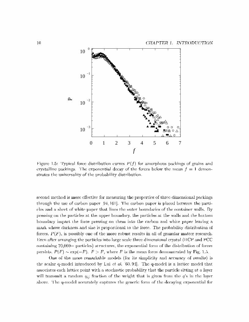
Figure 1.5: Typi al for e distribution urves P (f) for amorphous pa kings of grains and rystalline pa kings. The exponential de ay of the for es below the mean f = 1 demon-strates the universality of the probability distribution.se ond method is more e�e tive for measuring the properties of three dimensional pa kingsthrough the use of arbon paper [94, 161℄. The arbon paper is pla ed between the parti- les and a sheet of white paper that lines the outer boundaries of the ontainer walls. Bypressing on the parti les at the upper boundary, the parti les at the walls and the bottomboundary impart the for e pressing on them into the arbon and white paper leaving amark whose darkness and size is proportional to the for e. The probability distribution offor es, P (F ), is possibly one of the more robust results in all of granular matter resear h.Even after arranging the parti les into large s ale three dimensional rystal (HCP and FCC ontaining 70,000+ parti les) stru tures, the exponential form of the distribution of for espersists, P (F ) � exp(�F ); F > �F , where �F is the mean for e demonstrated by Fig. 1.5.One of the more remarkable models (for its simpli ity and a ura y of results) isthe s alar q-model introdu ed by Lui et al. [60, 94℄. The q-model is a latti e model thatasso iates ea h latti e point with a sto hasti probability that the parti le sitting at a layerwill transmit a random qij fra tion of the weight that is given from the q's in the layerabove. The q-model a urately aptures the generi form of the de aying exponential for

1.4. OUTLINE 11for es above the mean. Other models, su h as a ve tor generalization of the q-model [66℄, aptures the texture of the for e network, as do the ellipti or elasto-plasti models [224℄.1.4 OutlineThe overall purpose of my work is to study of granular materials that are subje ted to onstant energy inje tion through external driving. In Chapter 2 the experimental methodsutilized, the in lined plane with a vibrating sidewall, and a vibrating sau er, are des ribedin detail. Also, Chapter 2 reviews the methodologies of the a quisition and analysis ofhigh speed digital images with the goal of a urate parti le identi� ation and lo ation andtra king over extended times.Chapter 3 begins with a detailed review of the kineti theory of elasti and inelas-ti gases, as well as a omprehensive overview of the re ent numeri al methods utilized toreprodu e granular uids. I present a systemati experimental study of a two-dimensionalgranular gas of nearly identi al steel parti les that are onstrained to roll on a glass sub-strate. Many of the statisti al measures of kineti theory are evaluated from the experi-mental data. For example the distribution of path lengths and times between ollisions aremeasured dire tly and found to deviate signi� antly from the predi tions of kineti the-ory. Also, the distribution of parti le velo ities is measured for a range of densities andfound not to have a Maxwell-Boltzmann form. A simple experimental study is performedto test re ent theoreti al predi tions for the pressure balan e of a granular uid. Deviationsnear the point of energy inje tion are found to be the dominating deviation from a truehydrodynami treatment.In Chapter 4 the method utilized in Chapter 3 is employed to study pattern formationin a granular liquid. We demonstrate that the olle tion of parti les be omes unstable asthe a eleration of the driving for e is in reased. Above a riti al a eleration, the parti lesundergo free ight and return to the driving wall. If the driving parameters are su h thatthe layer return to the driving wall at the moment of maximum a eleration, then surfa epatterns will spontaneously form. The pattern is found to undergo a bifur ation to a perioddoubling regime where a se ondary surfa e instability an arise. We also demonstrate thethe layer an also form patterns at four times the period of the drive. The temperature ofthe layers is measured as a fun tion of the phase of the driving and is shown to demonstratesho k waves. Also, a position dependent orrelation fun tion is de�ned and is utilized, alongwith the velo ity �elds, to des ribe the wavelength and onset time of patterns. Insights intothe me hanisms for pattern formation are shown to be qualitatively di�erent than those ofNewtonian uids.In Chapter 5 the se ond method of energy inje tion, namely the sau er geometry, isutilized to study the a�e ts of additional intera tions in dilute granular gases. By embedding

12 CHAPTER 1. INTRODUCTIONa dipolar potential, a omplished by magnetizing the parti les, we observe that lustersspontaneously nu leate and grow. The number, size, and geometry of the lusters are foundto depend sensitively on the rate at whi h the kineti energy of the parti les is lowered. Wealso demonstrate that the growth rates of the lusters is hara terized by a single universalform whi h does not depend on the driving or density. We present a phase diagram that aptures the observed phenomenon, in luding a metastable phase that losely resembles atenuous network of polymer hains [33℄.In Chapter 6 we extend the previously presented ondition of simple spheri al parti lesto one with spatially anisotropi parti les. We �rst present a set of experiments thatdetermine the oeÆ ient of normal restitution of a rod on multiple surfa es at di�erentangles of in iden e. In the se ond experiment a one dimensional annulus is �lled withrods and shaken verti ally. We observe that the olle tion of rods will undergo dire tedmotion that is determined by both their angle of in lination and the velo ity of the drivingsignal. We present a simple model based on onservation of energy and onservation ofangular momentum that qualitatively aptures the dynami s of the rod system. Resultsfrom soft-rod mole ular dynami s is also presented and is shown to quantitatively apturethe experimental results [226℄. We utilize the results of this hapter to explain a more omplex phenomenon of vortex motion in our previous three dimensional experiments [37℄.In Chapter 7, a new system is investigated. The statisti al properties of a rumpledma ros opi membranes (paper) are investigated by using high resolution laser topography.By rumpling large sheets of paper and then unfolding them, a hierar hi al stru ture ofline-like ridges emerge. The distribution of the urvature and the lengths of the ridges aremeasured with te hniques adapted from geomorphology [238℄. We also present a Hurstanalysis of the surfa es and �nd that the sheet is self-aÆne. Our results are ompared to urrent theoreti al treatments of rumpled sheets [70, 237℄.We on lude with a des ription of the major results and dis uss the future work thatwill extend these studies in Chapter 8 and 9.
13Chapter 2Experimental MethodsThis hapter will serve a two-fold purpose. First, an introdu tion and review of the exper-iments performed on inelasti granular uids is given. Se ond, des riptions of the experi-mental pro edures and methods in addition to the preliminary data required to motivatethe results presented and dis ussed in Chapters 3, 4, and 5.2.1 Introdu tionA granular uid an only be produ ed by onstantly supplying external energy to ompen-sate for the loss of energy due to fri tion and inelasti ollisions between parti les and theboundaries. Therefore, a non-equilibrium steady state is attained only if the energy inputis balan ed by the energy loss. In granular uids ea h fundamental parti le or \mole ule"has many internal degrees of freedom that determine the inelasti ity of ea h parti le. Thatis, these internal modes are ex ited through ollisions and as a result transfer energy in theform of heat to the surroundings, therefore de reasing the energy of olliding parti les. Inideal uids, or situations where parti les undergo Brownian motion through the intera tionwith uid mole ules, a thermodynami temperature is well de�ned. However in granular uids the internal thermostat of ea h grain is e�e tively at T = 0.Dissipation in granular matter is manifest in essentially two forms: fri tion with sur-fa es and inelasti ity from ollisions. If the ow of grains is rapid, energy must be onstantlysupplied from an external sour e. Model experiments that are designed to investigate inelas-ti gases onsist of granular parti les inside ontainers where energy is ontinuously inje tedat a boundary [130, 167, 232℄. As a result of the driving asymmetry, gradients in both thedensity and the granular temperature are unavoidable onsequen es of experiments of thisnature. The presen e of gradients that may lead to large s ale ows must be a ounted forwhen omparing results to non-equilibrium kineti theory [86, 184, 220℄.

14 CHAPTER 2. EXPERIMENTAL METHODS2.2 Methods of Energy Inje tionUtilizing re ent advan es in high speed digital image a quisition, experimenters an a quirehigh resolution images of the positions of ma ros opi parti les at frame rates mu h fasterthen the mean free time between ollisions. Very pre ise measurements of the positions ofparti les between ollision events are now possible. However, at this time, parti le positionsand subsequently the velo ities an only be obtained a urately in two-dimensions by dire timaging, thus for ing ertain onstraints on the experimental geometry.One of the �rst experiments to investigate the statisti s of granular gases throughparti le tra king, utilized an apparatus in whi h the parti les are vibrated verti ally insidea narrow transparent slot [230{232℄, whi h we will denote as Method I. Warr et al. �rstreported Maxwellian statisti s for the velo ity omponents of the parti les parallel to theplane of the transparent side-walls. However, unavoidable lossy intera tions may arisefrom ollisions between parti les and the side-walls [231℄. Following this work, Wildmanet al. [236℄ were able to perform relatively long time parti le tra king to measure di�usion onstants by interpreting mean square displa ement data over a very broad range of density.More re ently, in a similar apparatus, Rouyer and Menon [192℄ report that their velo itydistributions fun tions (VDF) have a form that an be parameterized by a single variable,the granular temperature, and are thus presented as universal.Another method of energy inje tion utilizes a large at ontainer that is vibratedverti ally to ex ite a sub mono-layer of parti les [141,167,168℄. We will denote this methodas the sau er geometry. O�- enter ollisions are responsible for the motion of parti les inthe (x; y) plane; additionally, the presen e of perturbations in the driving surfa e and inthe parti les aids the randomization of parti le traje tories. Momentum is transfered tothe parti les from the driving surfa e through inelasti ollisions. If the magnitude of thedriving a eleration is larger than gravity,1 (g is parallel to the dire tion of the driving), theparti les may begin to move in straight lines with velo ities perpendi ular to the drivingdire tion. Inter-parti le ollisions are also inelasti and may o ur with multiple s enarios.Parti les an either ollide while in free- ight, or while one or both parti les are in onta twith the driving plate.The purpose of the methods des ribed above is to inje t energy su h as to produ ea two-dimensional \steady state" granular gas. The hoi e of a bi-dimensional geometryresults from the onstraint of dire t visualization through the use of digital imaging as themost a urate means to identify and tra k individual parti les. Both methods are a typeof verti al vibration against the a eleration of gravity. However, to understand the role of1The a eleration of the driving plate does not have to ex eed g = 980 m s�2 in order to initiate motion.If a parti le begins to roll on the surfa e, due to surfa e imperfe tions, lift-o� from the driving plate is notne essary to sustain parti le motion if a resonan e between the driving motion and the parti le motion isestablished.

2.3. DATA ACQUISITION AND ANALYSIS TECHNIQUES 15verti al vibration on the statisti al properties of granular gases, we hose to investigate thesystem that requires the least interpretation. The slot/in lined plane geometry allows fordire t visualization of parti le positions in both parallel and perpendi ular to the dire tionof energy inje tion whereas the sau er geometry the parti le motion in the dire tion ofdriving is lost due to the imaging.Another distin tion between the two methods is the level of intera tion between theparti les and the energy sour e. In both methods the parti les intera t, with ea h other ata frequen y given by � = 1=� =q2�hv2x;yi�� (2.1)where � is the mean ollision time, � is the parti le diameter and hvx;yi is the spatiallyand temporally averaged squared velo ity in the (x; y) plane. In the sau er geometry, theparti les intera t with the driving plate with frequen y on the order of the driving frequen y,�p = g2p3A!; (2.2)where A and ! are the amplitude and frequen y of driving, respe tively. However, inMethodI the intera tion between the parti les and the driving sour e is simply a fun tion of theoverall density and the inelasti ity of the parti les.We have utilized both methods to produ e granular uids. In Chapter 3, and in linedplane is utilized for the purpose of measuring a system that losely resembles an idealinelasti gas where parti les are traveling in paths that lead to inter-parti le ollision withminimal in uen e of external perturbations. In Chapter 5, a at sau er is utilized toprodu e a granular uid that resembles a olle tion of parti les di�using through sto hasti or Brownian motion. This method was also hosen to minimize spatial gradients indu edby gravity.2.3 Data A quisition and Analysis Te hniquesPrior to the dis ussion of experimental results or analysis the following se tion on erningthe methodologies and te hnology developed that make this experimental investigation pos-sible, are dis ussed. What will follow is a brief dis ussion of high speed imaging, and anoverview of the algorithms utilized to lo ate and tra k parti les. Most of the following willbe a review of the work of Cro ker and Grier [63℄. In Chapters 2, 4, 5, and 6 the methodsof high speed digital imaging and analysis dis ussed in this Se tion are utilized.2.3.1 High-speed Digital ImagingAs mentioned in Se tion 2.1, advan es in digital imaging have vastly improved in the pre- eding de ades. Con urrently, the density of storage medium (hard disks), random a ess

16 CHAPTER 2. EXPERIMENTAL METHODSmemory (RAM), and the density of transistors on mi ropro essors (CPU) have met or ex- eeded the empiri al fa t known as Moore's Law [156℄ for semi ondu tor te hnology.2 The ombination of these advan es has vastly improved the feasibility of a quiring, storing, andsubsequently pro essing digital images. The �rst harged oupled devi e (CCD) was devel-oped by George Smith and Willard Boyle at Bell Laboratories (now Lu ent Te hnologies)in 1969. The CCD itself is e�e tively a memory devi e that utilizes the photoele tri e�e tmanifest in ertain semi ondu tors. By sampling the presen e of ele trons in the potentialwells that omprise the pixels, known as integration, the intensity of the in oming light ismeasured for ea h pixel element. As with many te hnologies, quality and speed are oftenmutually ex lusive entities. However, in the re ent past, the te hnology of high resolutionCMOS ( omplementary metal oxide semi ondu tor) based CCD arrays ombined with highframe rates (upwards of 10,000 frames s�1) has triggered a se ond revolution in the a ura yof imaging of dynami al systems.For the experiments performed on granular materials, a Kodak Motion Corder (SR-1000) digital amera with a maximum spatial resolution of 512�480 pixels is used to a quireimages at a rate of 250 frames s�1. At this frame rate and resolution, 1365 onse utiveimages are bu�ered in on-board memory modules and then transfered through the SCSI(small omputer systems interfa e) bus onto a mi ro omputer for analysis. The analysisis performed using IDL (The Intera tive Data Language) and many routines have beenadapted, spe i� ally those of Cro ker, Grier and Weeks of Refs. [2, 63℄.2.3.2 Image Pro essingDigital image pro essing is a broadly varied subje t with appli ations in many dis iplinessu h as astronomy, medi ine, biology and physi s. The fundamental unit of digital data,representing a mapping of light intensity, is the pixel (voxel) in a real two- (three-) dimen-sional spa e. For all images in this work the pro essing is performed in two-dimensions withsquare pixels.In the work of Cro ker and Grier [63℄ �ve de�nitive steps to the pro essing of digitalimages of parti les are de�ned. Although the subje t of their interest were olloidal parti lesheld in suspension undergoing Brownian motion, the essential methodology is universal. Thestages of parti le tra king are des ribed as� Image Restoration� Lo ating parti le positions� Re�ning parti le lo ations2Moore's Law is usually reserved for mi ropro essor te hnologies, however similar \laws" have beenused to des ribe the advan es in the density of random a ess memory and storage medium, though theirpro essing speeds have lagged that of mi ropro essors.

2.3. DATA ACQUISITION AND ANALYSIS TECHNIQUES 17� Dis rimination of \false" parti les� Conne ting parti le positions in time to form traje toriesThe omplexity (i.e. the level of noise) of the a quired images determines the diÆ ultyasso iated with ea h step of the pro ess. Image restoration involves a \normalizing" of theimages to an ideal state. Most raw image data is not ideal due to the following ir um-stan es. Geometri distortions indu ed by lenses, long wavelength noise asso iated withinhomogeneous illumination and short wavelength noise brought on by digitization. Tominimize the geometri distortions we pla e the amera �3.5 m from the experiment andutilize a high quality 50mm lens. By illuminating with a high frequen y sodium vapor lightfrom nearly 2 m above the experiment a single bright spot is re e ted from the surfa e ofthe parti les that resolves to 5-7 pixels a ross ea h parti le on the CCD.We utilize a band-pass (see routine bpass.pro Appendix A) �lter that serves twopurposes. Lo ally, a Gaussian kernel, whose width is slightly larger than the size of the par-ti le in pixels, is onvolved with the image to removes short wavelength noise, additionallybox ar averaged ba kground is subtra ted to suppress long wavelength u tuations. On ethe image is properly re onstru ted and �ltered, the morphologi al pro ess known as dilateis performed. Dilation sets a pixel's value to the highest found within a spe i�ed distan e.If a pixel's value does not hange during the dilation pro edure it determined to be thebrightest pixel within it's neighborhood and is therefore a andidate for the lo ation of theapproximate enter. To re�ne the lo ation of the parti le enter to sub-pixel levels thebrightness weighted entroid is al ulated. The routine utilized for the pro ess des ribedabove is ontained in feature.pro.If the purpose of the analysis is to have a urate parti le lo ations for measuringstati stru tures then the following is unne essary. However, if the goal is to identify andlink parti le positions into traje tories then additional work is required. First, one musthave an a priori knowledge of ertain aspe ts of the parti les under onsideration. The �rstimportant parameter to onsider is the rate at whi h images are a quired as ompared tothe time it takes a parti le to travel it's own diameter. For example, if a 3 mm parti letravels for 1 m under the in uen e of gravity then a amera frame rate must be at least3000 frames s�1 in order to apture the parti le moving half it's diameter in two onse utiveimages. In most ir umstan es, there are multiple parti les within the view of the CCD andthe density an often rea h values near to the lose pa king limit. High densities also posea onsiderable hallenge when distinguishing parti les between frames. If these issues aretaken into a ount prior to the a quisition of data, then the following method for linkingtraje tories is appli able and eÆ ient. Fa tors su h as density, and high parti le velo itiesdemonstrate the importan e of high speed image a quisition at high spatial resolutions.Many experiments on granular gases are ondu ted with high speed ameras. However,
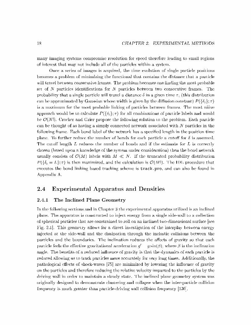
18 CHAPTER 2. EXPERIMENTAL METHODSmany imaging systems ompromise resolution for speed therefore leading to small regionsof interest that may not in lude all of the parti les within a system.On e a series of images is a quired, the time evolution of single parti le positionsbe omes a problem of minimizing the fun tional that ontains the distan e that a parti lewill travel between onse utive frames. The problem be omes one �nding the most probableset of N parti les identi� ations for N parti les between two onse utive frames. Theprobability that a single parti le will travel a distan e Æ in a given time � , (this distribution an be approximated by Gaussian whose width is given by the di�usion onstant) P (fÆig; �)is a maximum for the most probable linking of parti les between frames. The most n�aiveapproa h would be to al ulate P (fÆig; �) for all ombinations of parti le labels and wouldbe O(N !). Cro ker and Grier propose the following solution to the problem. Ea h parti le an be thought of as having a simply onne ted network asso iated with N parti les in thefollowing frame. Ea h bond label of the network has a spe i�ed length in the position timeplane. To further redu e the number of bonds for ea h parti le a uto� for Æ is assumed.The uto� length L redu es the number of bonds and if the estimate for L is orre tly hosen (based upon a knowledge of the system under onsideration) then the bond networkusually onsists of O(M) labels with M � N . If the trun ated probability distributionP (fÆi = Lg; �) is then maximized, and the al ulation is O(M !). The IDL pro edure thatexe utes the bond linking based tra king s heme is tra k.pro, and an also be found inAppendix A.2.4 Experimental Apparatus and Densities2.4.1 The In lined Plane GeometryIn the following se tions and in Chapter 3 the experimental apparatus utilized is an in linedplane. The apparatus is onstru ted to inje t energy from a single side-wall to a olle tionof spheri al parti les that are onstrained to roll on an in lined two-dimensional surfa e [seeFig. 2.1℄. This geometry allows for a dire t investigation of the interplay between energyinje ted at the side-wall and the dissipation through the inelasti ollisions between theparti les and the boundaries. The in lination redu es the a�e ts of gravity so that ea hparti le feels the e�e tive gravitational a eleration g0 = g sin(�), where � is the in linationangle. The bene�ts of a redu ed in uen e of gravity is that the dynami s of ea h parti le isredu ed allowing us to tra k parti les more a urately for very long times. Additionally, thepathologi al e�e ts of sho k-waves [75℄ are minimized by lowering the in uen e of gravityon the parti les and therefore redu ing the relative velo ity imparted to the parti les by thedriving wall in order to maintain a steady state. The in lined plane geometry system wasoriginally designed to demonstrate lustering and ollapse when the inter-parti le ollisionfrequen y is mu h greater than parti le-driving wall ollision frequen y [130℄.

2.4. EXPERIMENTAL APPARATUS AND DENSITIES 19
Fcn. Gen.Amplifier
Computer
Camera
Solenoid
x
−y
β
Figure 2.1: S hemati diagram of the in lined plane experimental setup. The in lined planeis a smooth glass surfa e, the side-walls and driving wall are stainless steel so that theparti le-boundary ollisions approximate those between parti les. The driving is produ edby os illating the lower side-wall by means of a solenoid. The angle of in lination �, an bevaried from � = 0� 8 degrees, the values of � used are 2Æ � 0:1Æ, and 4Æ � :1Æ.

20 CHAPTER 2. EXPERIMENTAL METHODS
Driving Wall
30 cm
19 cm
(a)
(b)
(c)
Figure 2.2: Images of the system taken from above. The top left orner is onsidered theorigin of our oordinate system (0; 0). (a) The system in the gas regime (Nl = 1) (b) aliquid regime (Nl = 10) The white bars allow us to tra k the position of the driving wall,shown by the solid white line in (a). ( ) The system when the enter of mass be omesphase lo ked to the driving wall. Under ertain driving and density onditions standingwave patterns arise (see Chapter 4).

2.4. EXPERIMENTAL APPARATUS AND DENSITIES 21The experimental on�guration onsists of a 100 d � 60 d (30 m � 19 m ) glassplane that is in lined at an angle � with the horizontal. The parti les are stainless steel withdiameter d = 3:175 mm and a high degree of spheri ity (Æd=d = 10�4). The energy sour eis an os illating side-wall, driven by a solenoid, that is lo ated as shown in Fig. 2.1(a).The driving signal is a 10 Hz pulse with a velo ity during ea h pulse of � 40 m s�1.The driving frequen y and amplitude were hosen to ensure that no phase dependen e onthe enter of mass is observed. However, at frequen ies below 4 Hz (in the range of �used for these experiments) the parti le positions are phase-lo ked with the driving and apatterns may be observed (see Fig. 2.2 and Chapter 4). The driving signal is produ edwith a omputer interfa ed Aglient Te hnologies 33120-A wave-form generator that is andsubsequently ampli�ed by an HP 6824A Ampli�er. The in lination of the plane an bevaried between � = 0Æ � 8Æ, for our experiments the angle was �xed at � = 2Æ � 0:1Æ,4Æ� 0:1Æ. In the extreme ase of � � 1Æ, the parti les essentially ease to intera t with thedriving wall and luster at the opposing boundary.2.4.2 Area Fra tion and Density Pro�lesAs with any granular system driven into a uidized state, large s ale gradients in the densitywill be present due to the inelasti ity of the grains, and the asymmetry of the driving withrespe t to gravity. The time averaged distribution of parti le positions is measured bynarrowly binning the system perpendi ularly to the axis of interest and measuring the ratioof the fra tion of the parti le areas within the bin to the bin area. By averaging over thewidth of ea h bin the density distributions are re overed for both the x; y dire tions. Thedensity in the x; y-dire tions �(x), �(y) are shown in Fig. 2.3.In previous experimental systems, [142, 231℄ where parti les are vibrated into gasstate by a side-wall, the density distribution was �t to a Boltzmann distribution indi atingan isothermal atmosphere, �(y) = �oe�gy=T : (2.3)However, our results for the density distribution show a fundamentally di�erent result. InFig. 2.4(a), the data displayed in Fig. 2.3(b) is plotted on a log-log s ale. The tails of thedensity distribution are found to follow a power law de ay of the form,�(y) = �o y��; (2.4)where we observe empiri ally that � � Nl (viz. the number of layers determines the exponentof the de ay). Figure 2.4(b) displays the linear dependen e of � on Nl. The la k ofexponential tails implies that the law of isothermal atmospheres breaks down for granularsystems as we shall also see when we dis uss the s aling of the granular temperature andthe granular equation of state in Chapter 3.

22 CHAPTER 2. EXPERIMENTAL METHODS(a)
x(cm)
ρ(x
)
302520151050
0.4
0.3
0.2
0.1
0
Nl = 5, β = 4Nl = 4, β = 4Nl = 4, β = 2Nl = 3, β = 2Nl = 2, β = 2Nl = 1, β = 2(b)
y(cm)
ρ(y
)
20151050
100
10−1
10−2
Figure 2.3: (a) The density �(x) versus x for all Nl. The obvious lustering due to inelasti ollisions at the side-walls is demonstrated here. Also, as Nl is in reased the system be omesmore inhomogeneous in a ross the ell. This e�e t is most likely due to the onset of lusteringinstabilities that have been re ently dis ussed [15, 120, 138℄. (b) The aerial density plots�(y) for ea h Nl and � on a log-linear plot. The area fra tion � is measured by integrating�(y) over that region of interest. The total are under ea h urve orresponds to the averagearea fra tion for that parti ular Nl.

2.4. EXPERIMENTAL APPARATUS AND DENSITIES 23Nl = 5Nl = 4Nl = 3Nl = 2Nl = 1
(a)
y (cm)
ρ(y
)
102101
100
10−1
10−2
10−3
(b)
Nl
Λ
6543210
6
5
4
3
2
1
0Figure 2.4: (a) The density distribution �(y) vs y on a log-log plot. The dashed lines arepower-law �ts (see Eq. 2.4) for the tails of the distributions. (b) De ay exponents for thedensity plots shown in (a). The dashed line is simply a line with slope one and inter eptzero.

24 CHAPTER 2. EXPERIMENTAL METHODSNl � � Np1 2.0 0.022 1002 2.0 0.068 2003 2.0 0.138 3004 2.0 0.191 4004 4.0 0.302 4005 4.0 0.581 500Table 2.1: Experimental values of the number of layers Nl, the angle of in lination �, andthe resulting measured value of �. Np the number of parti les in the system is given for larity.The results presented in the following Chapter will be given in terms of the numberof single layers a ross the ell, Nl and the angle of in lination �, whi h determine theaveraged area fra tion � [see Table 2.1℄. The number of parti les within the ell, measuredin number of mono-layers Nl a ross the driving wall, is varied between Nl = 1{5, (viz. fromNp = 100{500 in steps of 100 (where Np is the number of parti les). The area fra tion ismeasured by �rst de�ning a region of interest (ROI) that is entered about the maximumof the aerial density �(y), with a limited extent in the y-dire tion that overs �10% of �(y).The ROI s heme also ex ludes all parti les that are within 3d of the side-walls to ensurethat lustering due to the side-walls does not aversely a�e t the results. The over-plottedbox in Fig. 2.1(b) demonstrates the ROI de�nition for � = 0:13. The time averaged valueof � is measured by omputing,� = 1� �Xt=0 NXi=1 �d2Æ(r � ri(t))4AROI ; (2.5)where AROI is the area of the region of interest and ri(t) is the parti le position within theROI at time t.2.4.3 The Sau er GeometryWe have also hosen to utilize the apparatus des ribed as the sau er geometry in Chapter 5.We note that although this experiment does not allow for a straight forward separationbetween the in uen e of driving and the inter-parti le ollisions due to an inability tovisualize the z-dire tion, in the dilute limit spatial gradients in the density are minimizedin the (x; y)-plane. Therefore, this system is ideal for investigating athermal systems asma ros opi models of systems des ribed by a system in the presen e of a heat bath.The experimental apparatus onsists of a Labworks ET-139 ele trodynami shakerthat is driven by a PA-141 power ampli�er. The shaker is rigidly mounted in an aluminum

2.4. EXPERIMENTAL APPARATUS AND DENSITIES 25
a
b
c
ed
f
gFigure 2.5: (a) S hemati diagram of the experimental setup des ribed used for variousexperiments su h as those performed in Chapters 5 and 6. The labeled items in lude: aThe ele tro-me hani al shaker assembly. b The supporting base that is parallel to the uppersupport base and held �xed by three onne ting rods. The semi- exible onne ting shaftmade from 1/8" G-10 that ouples the shaker to the shaft ridged shaft. d The ridged keyedshaft that rides within the linear bearing. e The linear roller bearing that is aÆxed tothe upper support plate. f The mounting plate that allows for multiple experiments to beinter hanged. g Leveling s rews that allow for leveling to 0:01 mm.

26 CHAPTER 2. EXPERIMENTAL METHODSbase ontainer shown s hemati ally in the top panel of Fig. 2.5. The bottom plate of the base ontainer, denoted (b) in the s hemati , has three leveling s rews (5=800 � 80) that allow forpre ise ontrol of the in lination of the assembly. The top plate of the assembly is onne tedvia three posts to the bottom plate and are aligned to within 0.01". Mounted dire tly abovethe enter of the shaker is a ridged linear me hani al bearing (e). The keyed shaft, (d) ismounted to the shaker via a \weak-link" ( ) exible onne tion that ensures (produ edfrom 1/8" G-10) that any deviation in the z-dire tion of the shaker does not me hani allybind the bearing. The mounting platform (f) is onne ted to the keyed shaft and allowsfor multiple experimental ells to be inter hanged. The driving signal originates from anAglient Te hnologies 33120-A wave-form generator wave-form generator that is omputer ontrolled via an IEEE-488 (GPIB) interfa e. The a eleration of the plate is monitoredand maintained through a 10 mV/g a elerometer that is rigidly onne ted, along the z-axis, to the underside of the mounting platform. The output signal from the a elerometeris fed into a EG&G lo k-in ampli�er that is also GPIB ontrolled. The lo k-in signal aswell as the waveform generator are simultaneously interfa ed and ontrolled via a LabViewprogram that an ouple the signals through a feedba k loop for pre ise maintenan e of thedriving signal.2.4.4 Average Density DistributionsIn the sau er geometry, the overing fa tion is uniquely de�ned ratio of total parti le areaand the total surfa e area, � = � d2R �2 NXi=1 Æ(r � ri); (2.6)where R is the radius of the ontainer. Although Eq. 2.6 serves well as a working de�nitionof the overing fra tion, the long-time averaged overing fra tion with preserved spatialinformation, �(r) = 1� �Xt=0( d2R )2 NXi=1 Æ(r� ri); (2.7)demonstrates that slight inhomogeneities still persist even after averaging (1 � 5) � 104instantaneous density distributions [see Fig 2.6℄.2.5 Long Time Parti le Tra king2.5.1 Parti le CollisionsIn the following se tions the long time tra king methods dis ussed in Se . 2.3.2 will beutilized to measure the e�e tive oeÆ ient of normal restitution. Figure 2.7(a) shows a
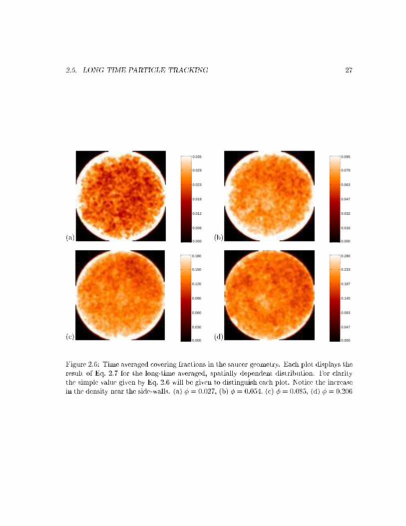
2.5. LONG TIME PARTICLE TRACKING 27
(a)
0.000
0.006
0.012
0.018
0.023
0.029
0.035
(b)
0.000
0.016
0.032
0.047
0.063
0.079
0.095
( )
0.000
0.030
0.060
0.090
0.120
0.150
0.180
(d)
0.000
0.047
0.093
0.140
0.187
0.233
0.280
Figure 2.6: Time averaged overing fra tions in the sau er geometry. Ea h plot displays theresult of Eq. 2.7 for the long-time averaged, spatially dependent distribution. For laritythe simple value given by Eq. 2.6 will be given to distinguish ea h plot. Noti e the in reasein the density near the side-walls. (a) � = 0:027, (b) � = 0:054, ( ) � = 0:085, (d) � = 0:206

28 CHAPTER 2. EXPERIMENTAL METHODS(a)
x (cm)
y(c
m)
76543210
7
6
5
4
3
2
1
0
(b)
y = 57
x2
2v2x
g sin(β)
x (cm)
y(c
m)
12111098
11
10
9
8
Figure 2.7: (a) Linked parti le positions over 1365 time steps (Nl = 3). Collision events aredetermined with a high degree of a ura y from traje tories su h as this. (b) The paraboli path of a single parti le. We use �xed values for vx and g = 980 m s�2 to measureg0 = 57g sin�. The �t gives � = 2:2Æ, the deviation from the measured value of � is 9%,whi h represents the la k of a ura y in the measurement of �.

2.5. LONG TIME PARTICLE TRACKING 29single parti le tra ked for 1365 time steps (5.46 se ). In subsequent hapters, long timetra king will also be used to test the validity of gas kineti theory.We identify ollision events from the traje tories by using the following algorithm.� Constru t velo ities� Sequentially ompare velo ity ve tors for hanges� Che k lo al neighborhood for a s attering parti le� If no s atterer he k for boundaryVelo ities are onstru ted as �nite di�eren es vj = �x�t , where �x = x(tj) � x(ti) and thesubs ripts i; j represent positions separated by the time di�eren e �t = 4ms. All velo ityve tors are ompared sequentially to �nd dire tion hanges given by = os�1(v̂i � v̂j); (2.8)where v̂ = v=jvj is the unit ve tor of the al ulated velo ity. If 20Æ � � 180o theproximity of all parti les at the same time instant is he ked. If a parti le is found within aradial distan e d+�d, whose velo ity also satisfy Eq. (2.8) it is onsidered as a andidatefor a ollision. To ensure that re- ollisions are not o urring, we maintain a re ord of theidentity of the previous ollision partner so that pairs an re- ollide if and only if one of thepartner parti les has undergone a ollision with yet a third parti le. If parti les pass theserequirements then a ollision has o urred. To extend the algorithm to in lude ollisionswith the boundary walls we �rst he k if Eq. (2.8) is satis�ed. We then he k if the parti le's enter is within d+�d of a boundary and it's velo ity omponent perpendi ular to the wallis reversed.2.5.2 CoeÆ ient of Restitution and Inelasti ityThe loss of energy in a ollision is de�ned as the inelasti ity whi h itself is determined by the oeÆ ient of restitution of the parti les. The value of the restitution oeÆ ient is a materialproperty of the parti les with a typi ally quoted value for a steel sphere as � � 0:9. If tworough, (i.e. fri tional) parti les with diameters d ollide in spa e, the relative velo ity ofthe pair at onta t an be modeled by,v12 = v1 � v2 � d(!1 + !2)� d̂; (2.9)where v and ! are the translational and angular velo ities respe tively [see Fig. 2.8℄, andthe subs ripts denote the parti le number, and d̂ is the unit ve tor that points along the line

30 CHAPTER 2. EXPERIMENTAL METHODSv
2v
2v
1v
ω
ω1
2
*
*
1d
v
vd
12
12*
Figure 2.8: (a) S hemati diagram of the a model for the ollision between two parti les within oming (outgoing) linear velo ities v1;2; (v�1;2), and angular velo ities !1;2, d is the ve tor onne ting their enters. (b) Geometri interpretation of an inelasti ollision between twosmooth parti les. The ve tors v12; v�12 are the relative velo ities at ollision. The dashedline indi ates the angle of the outgoing ve tor if the ollision was elasti . An in rease ofthat angle parameterizes the amount of inelasti ity.that onne ts their enters. The hange in the normal omponents of the relative velo ities,after a ollision v�12 � d̂ = �� (v12 � d̂); (2.10)and similarly, v�12 � d̂ = � (v12 � d̂); (2.11)for the tangential omponents, where �, are the normal and tangential omponents ofrestitution respe tively. The physi ally meaningful ranges of these parameters are � � 1and �1 � � 1. When � = 1, the ollision onserves energy. Therefore, any value < 1is said to be dissipative. If � = �1 the parti les are onsidered in�nitely smooth, and onversely for = 1 the parti les are ompletely sti ky. Using momentum onservation andthe restitution oeÆ ients ollision rules are de�ned as [146, 147℄,v�1 = v1 � (1 + �)2 vn � q(1 + )2q + 2 (vt + vr) (2.12)v�2 = v2 + (1 + �)2 vn + q(1 + )2q + 2 (vt + vr) (2.13)d2!� = d2! + 1 + 2q + 2[d̂� (vt + vr)℄; (2.14)

2.5. LONG TIME PARTICLE TRACKING 31where q is de�ned by the moment of inertia I of the parti les q = 4I=md2 and,vn = [v12 � d̂℄d̂ (2.15)vt = v12 � vn (2.16)vr = d2(!1 +!2)� d̂: (2.17)Above, vn and vt are the normal and tangential omponents of v12 due to translation,and vr is the tangential omponent due to rotation. M Namara and Luding [146,147℄ havedes ribed the la k of energy equipartition between the linear and rotational degrees offreedom for olliding rough parti les using this model for parti le intera tions.The omponents of the angular velo ity of the parti les, (both from spin indu ed bythe substrate and about the normal indu ed by ollisions) annot be resolved expli itly inour experiments. Therefore, while we observe the e�e t of the subtle interplay between thetransferen e of linear and angular momenta during ollisions, resolution of the ontributionsto ea h degree of rotational freedom is unattainable. Upon removing the angular velo itydependen e from the above equations the normal equations for the normal omponents arefound. Equation 2.10 is un hanged and Eqs. 2.12 and 2.14 take on the simple forms,v�1 = v1 � (1 + �)2 vn (2.18)v�2 = v2 + (1 + �)2 vn: (2.19)The re e tion law for the relative velo ities given in Eq. 2.10 determines the normal om-ponent of restitution in terms of the relative velo ity ve tors. Using the pro ess of ollisionidenti� ation des ribed in Se . 2.5.1, measurements of the normal omponents of the rel-ative velo ities of two olliding parti les events are made, revealing the e�e tive normal oeÆ ient of restitution, �e� = �(�v�12 � d̂)(�v12 � d̂) ; (2.20)where the over-bar denotes average over three pre/post- ollisional velo ities measured inthe ROI des ribed in Se . 2.4.1 [see Fig. 2.1(b)℄. The angle between the relative velo itiesof two olliding parti les is given by� = os�1(�v12 � �v�12); (2.21)parameterizing ea h ollision event [see Fig. 2.8℄.Thus, the oeÆ ient of restitution an be parameterized by the angle �. The prob-ability distributions P (�) for 60Æ � � � 180Æ for Nl = 1 � 5 ;� = 2 � 4, (see aption) areshown in Fig. 2.9(a{f). Data for � < 60Æ su�ers from a la k of statisti s and therefore is not

32 CHAPTER 2. EXPERIMENTAL METHODS
0.0 0.5 1.0 1.5 2.0α
6080
100120140160
θ(de
g.)
0.000.020.040.06
P(α
)
0.0 0.5 1.0 1.5 2.0α
6080
100120140160
θ(de
g.)
0.00
0.02
0.04
0.06
P(α
)
0.0 0.5 1.0 1.5 2.0α
6080
100120140160
θ(de
g.)
0.00
0.04
0.08
P(α
)
0.0 0.5 1.0 1.5 2.0α
6080
100120140160
θ(de
g.)
0.000.020.040.060.08
P(α
)
0.0 0.5 1.0 1.5 2.0α
6080
100120140160
θ(de
g.)
0.000.040.080.12
P(α
)
0.0 0.5 1.0 1.5 2.0α
6080
100120140160
θ(de
g.)
0.000.040.080.12
P(α
)(a)
(c)
(e)
(d)
(b)
(f)
Figure 2.9: The distribution of the normal omponent of restitution � versus 60Æ � � �180Æ, the relative angle of in iden e between parti le velo ities. (a) Nl = 1 ; � = 2:0, (b)Nl = 2 ; � = 2:0, ( ) Nl = 3 ; � = 2:0, (d) Nl = 4 ; � = 2:0, (e) Nl = 4 ; � = 4:0, (f)Nl = 5� = 4:0. The value of the z-axis for ea h graph is the probability of a ollision givinga value of � in a range of � +��, where �� = 2Æ.

2.5. LONG TIME PARTICLE TRACKING 33(a)
φ
〈α〉
0.60.50.40.30.20.10
0.9
0.8
0.7
0.6
0.5
0.4
(b)
η
P(η
)
1010.1
102
101
100
10−1
10−2
10−3
10−4Figure 2.10: (a) The mean value of the distributions of � shown in Fig. 2.9 averaged over60Æ � � � 180Æ, as a fun tion of the average overing fra tion �. The bars indi ate thespread in the distribution. (b) The distribution of energy inelasti ities given by Eq. (2.22)for (�)Nl = 1 ; � = 2:0, (�)Nl = 2 ; � = 2:0, (M)Nl = 3 ; � = 2:0, (�)Nl = 4 ; � = 2:0,(2)Nl = 4 ; � = 4:0, (Æ)Nl = 5� = 4:0. Ea h distribution is shifted verti ally for larity.

34 CHAPTER 2. EXPERIMENTAL METHODSin luded. Ea h graph represents the probability of the inelasti ity having a value � for arange of �+��, where �� = 2Æ. P (�) follows a very broad distribution of values over all �,and have a de reasing mean value as fun tion of � [see Fig. 2.10(a)℄. Thus, we observe thatthe oeÆ ient of restitution an have a broad distribution of values for the same impa tangle �.We also measured the energy loss due to a ollision as a fun tion of Nl �. The ratioof the magnitudes of the relative velo ities before and after a ollision,� = j�v�12jj�v12j ; (2.22)determines the energy restitution oeÆ ient, (�2 = �2 if all � are averaged). Figure 2.10(b)shows the distributions of measured values of � shifted for larity. We observe that a peakexists at a value onsistent with �2. Furthermore there exists a power law tail for values of� > 1, whi h has been interpreted as a random inelasti ity [21℄. The appearan e of a tailat high � implies that the rotational degrees of freedom are a tively transferring energy totranslational motion during a ollision.2.6 Dis ussionIn this Chapter, an introdu tion to the experimental approa h to studying granular uidswere given in detail. The methods of digital image pro essing as well as the algorithmsutilized to lo ate, label and tra k parti les over long times were dis ussed. We have in-trodu ed two model systems that di�er in their methods of driving. The system know asthe in lined plane will be explored further in the following hapter. We have hara terizedthe form of the density distributions as well as the dynami s of ollision events throughthe effe tive oeÆ ient of normal restitution and the inelasti ity. The system known asMethod II will be utilized in Chapter 5 to investigate the e�e ts of additional intera tionson phase transitions of granular gases.
35Chapter 3The Statisti s of Inelasti GasesIn the pre eding Chapter, the experimental systems utilized to study driven granular ma-terials were detailed. Two distin t experimental methods were presented as the prominentmodel systems that test granular kineti theories. In this Chapter, we will ontinue with theanalysis of the previously introdu ed experiments in the ontext of testing the developmentsof the kineti theory of inelasti gases. In addition, due to the proliferation of high speed omputing modeling of model granular systems, omparisons to the growing literature of omputer \experiments" are also made.Spe i� ally, this Chapter in ludes a detailed analysis of the velo ity distributions, thetemporal and spatial orrelations of both the positions and the velo ities of the parti les.Two fundamental tenets of gas kineti theory, the distributions of path lengths and freetimes (leading to the mean free path and time), are experimentally measured and found todeviate from the distributions for elasti parti les.3.1 Introdu tion to Kineti Theory3.1.1 Elasti Gases and FluidsThe goal of kineti theory is to des ribe the observable ma ros opi phenomenon of uidsthrough a detailed knowledge of the intera tions of of lassi al mole ules. However, asposed, the task at hand seems to be the integration of Newton's equations for 1023 parti lesper mole; this is itself an intra table problem. Therefore, a statisti al approa h must beadopted. In order to make the statisti al analysis tra table means that a detailed knowledgeof the initial onditions must be unne essary. Ignoran e to the minutiae for ea h parti le isplausible on physi al grounds i.e. the vis osity of a uid should not depend on the initialvelo ity of a single mole ule. In uids where the mean parti le separation is large omparedto the size of a parti le, known as a dilute gas, parti les move in straight lines and intera t
36 CHAPTER 3. THE STATISTICS OF INELASTIC GASESvia binary ollisions. The ollision pro ess an be modeled as two intera ting spheresthat onserve both energy and momentum during the intera tion. The number of ollisionevents between parti les depends on the density and temperature of the gas. Therefore,due to the enormity of the number of parti les within even a very dilute uid, a statisti alinterpretation, based upon the me hani s of binary ollisions, is well suited to bridge thedivide between mi ro- and ma ros opi dynami s.The foundation of what is known as kineti theory1 was �rst formulated by Maxwellin 1866 [145℄ with his introdu tion of the mathemati al derivation (though not onsideredto be mathemati ally rigorous) of the distribution of mole ular velo ities f(r;v; t). In 1872,Boltzmann introdu ed his H-theorem [38℄, where he extended the generality of Maxwell'sresult to a system of parti les whose velo ities are initially non-Maxwellian that when leftto evolve indeed return to the form proposed by Maxwell.Using f(r;v; t) as the fundamental quantity for the statisti al des ription of thesystem we an as ribe the number of parti les in the element of phase spa e (r; r+dr),(v;v+dv) as f(r;v; t)drdv ,where r and v are the position and velo ity. If the form of thefundamental distribution fun tion is known then averages over of mi ros opi variables anbe taken to yield ma ros opi quantities,�(r; t) = 1n Z f(r;v; t)�(r;v; t)d ; (3.1)where n = R fdv is the number density.The eventual result that we are striving for is the form distribution fun tion for thevelo ities of the parti les. Therefore, the time evolution of f(r;v; t) must be derived. Thepro esses that hange the distribution are due to the ollisions between parti les. Colli-sions serve two purposes, namely s attering parti les into and out of phase spa e elements.Therefore the time evolution of f(r;v; t)�f�t + v � rrf + F � rvf = � f�t (3.2)where F is the a eleration due to external sour es. The two sides of Eq. 3.2 determinethe motions of parti les through: (LHS) any spatial hanges due to velo ities and hangesof velo ities due to external for es { streaming operator, (RHS) hanges of the distributionfun tion due to ollisions between parti les.Averages (see Eq. 3.1) are obtained by integrating the distribution fun tion over thema ros opi variable of interest. Therefore, to derive the equations of motion for the ma ro-s opi variables of interest, ea h term in Eq. 3.2 is multiplied by �(r;v; t) and integratedover dv, �n��t = �rr � n�v + n����t + v � rr�+ F � rv��+��; (3.3)1This review of the kineti theory of elasti gases follows the dis ussion give by Bizon [26℄ and Chapmanand Cowling [55℄.
3.1. INTRODUCTION TO KINETIC THEORY 37again n is the number density and the last term on the RHS represents the rate of hange of� through ollisions whose value is zero for any onserved quantity. By onsidering the par-ti les as ideal (i.e. point-like), in d dimensions, there exist 2+d onserved quantities: mass,the d-momentum, and the kineti energy. By substituting these quantities into Eq. 3.3, thethree ontinuum equations for parti le motion are de�ned immediately,�n�t +rr � (nv) = 0 (3.4)n v�t + nv � rrv = �rrP (3.5)n�T�t + nv � rrT = �(2=d)(rr � q+P � rrv); (3.6)where P is the pressure tensor, q is the heat ux and T is the temperature. The beauty ofthese equations is that no knowledge of the form of f(r;v; t) or the details of the ollisionpro esses were required, only that the three fundamental quantities were onserved.However, this does not imply that everything is known by having Eqs. 3.5{3.6. Whatis la king is the dependen e of the pressure tensor and the heat ux ve tor to the quantitiesn; v; T . Therefore, to derive the onstitutive relations, and subsequently the form off(r;v; t), a detailed knowledge of the ollision pro ess is required.If the gas onsidered dilute then only binary ollisions are assumed to o ur. Without onsidering the entire derivation of the kinemati s of ollisions between parti les the rateof hange of the distribution fun tion an be expressed as�f�t +v�rrf+F�rvf = Z Z [f (2)(r;v01;v02; t)�f (2)(r;v1;v2; t)℄dD�1(v12 �d̂)dDdv2: (3.7)The LHS of Eq. 3.7 is the identi al form of Eq. 3.2 with the RHS repla ed by the integralsover the two parti le distribution fun tion f (2)(r;v1;v2; t). The primes denote post- ollisionvelo ities, d is the parti le diameter, d̂ is the unit ve tor that onne ts the enters of theparti les, v12 = v2�v1 is the relative velo ity of the olliding parti les and d is the angularelement that des ribes the geometry of the ollision in d-dimensions. Instead of having anunknown onstitutive relation, the la k of losure is shifted to the two parti le distributionfun tion f (2).To lose the equations and, subsequently determine f (2), Boltzmann made his famous onje ture, or the Stosszahlansatz, known today as the mole ular haos assumptionf (2)(r;v1;v2; t) = f(r;v1; t)f(r;v2; t): (3.8)By dire t substitution, of Eq. 3.8 into Eq. 3.7 the Boltzmann equation for mole ular trans-port is found. Using his H-Theorem [38℄ Boltzmann rigorously solved for the distributionfun tion that Maxwell had earlier proposed based on very simple arguments (see Se . 3.5),
38 CHAPTER 3. THE STATISTICS OF INELASTIC GASESnamely the Maxwell-Boltzmann distributionf = n(2�T )�d=2 e(v�v)2=2T : (3.9)Boltzmann's mole ular haos assumption assumes that orrelations, due to ollisionsor ex luded volume, do not exist. There is long standing onsensus [55℄ that the assumptionof zero orrelation is not founded. To ompensate for orrelations brought upon by in reaseddensity, and the �nite size of parti les, Eq. 3.8 has been modi�edf (2)(r;v1;v2; t) = g(d; �)f(r2 � dd̂;v2; t)f(r1 � dd̂;v1; t): (3.10)The form of the pair orrelation fun tion g(d; �) will be ome important in determining theequation of state and will be dis ussed further in Se s. 3.2 and 3.7.3.1.2 The Addition of Inelasti ityIn an attempt to quantify the behavior of rapid granular ows, the kineti theories ofideal gases introdu ed by Boltzmann (see above), later reworked by Chapman and Enskog,have been modi�ed. These well established theories have been transmuted from des ribinggases of smooth, �nite, ideal parti les, to systems of parti les with both �nite volume anddissipative ollisions, referred to as granular gases. Early theories, [95, 114℄ assumed thatthe parti le's velo ities were des ribed by a Maxwellian distribution and that mole ular haos was also obeyed and that the parti les ould be modeled as a dissipative ontinuum uid. Most kineti theories of granular gases assume that the parti les are homogeneouslydriven into a steady state. However, as dis ussed in Chapter 2 and further dis ussed herein,homogeneous heating is experimentally impossible to a hieve. Gradients in both the tem-perature and the density will always exist. In a set of re ent works Kumaran [132℄ andSunthar and Kumaran [206℄ have developed a kineti approa h to both dilute and densegranular matter driven from a boundary wall, similar to Method I. The formalism requiresthat three fundamental assumptions be made. First that the distribution of parti le velo -ities is Maxwell-Boltzmann. Se ond that the driving wall move less than the diameter of aparti le. And lastly, that the oeÆ ient of restitution is very lose to unity.In Refs. [132, 206℄ it is assumed that the Boltzmann equation (see Eq. 3.7) is validfor a granular gas. The inelasti ity between grains is a �xed value that enters the analysisthrough the leading order dissipation rateRd = �1=2rN2gT 1=2(1� �2); (3.11)where � is the inelasti ity of the parti les, g is the a eleration due to gravity and r = d=2.The energy is inje ted to the parti les by assuming that there exists a periodi ally os illating
3.1. INTRODUCTION TO KINETIC THEORY 39energy sour e lo ated at the inferior wall that ontributes to an energy inje tion rate thatis to �rst order given by the granular temperature and the velo ity of the driving wallS = � 2��1=2 NgT 1=2U2; (3.12)where N is the number of parti les per unit length a ross the driving wall.Using an asymptoti analysis approa h the authors derive a form for the s aling ofthe temperature, anisotropy of temperature, and the density as a fun tion of distan e fromthe driving. Their theoreti al results ould be veri�ed by our observations, that follow inthe Se tions below.3.1.3 Computer Experiments of Model Granular SystemsOne of the earliest indi ations that inelasti ity may be manifest in the velo ity distributionfun tion (VDF) of is due to Goldhirs h et al. [86℄. The authors performed a mole ulardynami s simulations (MD) on a system of parti les whose initial state was a homogeneouselasti gas with sto hasti driving. At a parti ular instant, the sto hasti driving wasremoved and inelasti ity was turned on. The authors observed that the kurtosis of thevelo ity distribution in reased as the system of parti les be ame more lustered. UsingMD simulations van Noije and Ernst, along with Triza and Pagonabarraga [170,221℄ haveexamined both large and short-s ale stru ture in a system of grains driven by a random for eat onstant inelasti ity. Additionally, Refs. [26, 30, 174℄, also report long range orrelationsin positions, densities and velo ities arise at s ales mu h longer than the mean free pathof the parti les. As mentioned above, Pagonobarraga et al. [170℄, and Soto et al. [204℄,have arefully investigated the e�e t of in reasing � on the short range stru ture of thegas. They report a very noteworthy result, that is the breakdown of the mole ular haosassumption with an in rease in � and density. The Enskog orre tion (see Eq. 3.10), andthe pair orrelation fun tion, g(r), in general assume nothing about possible orrelationsbetween parti le positions and velo ities prior to a ollision event. The generalized pair orrelation fun tion �(�) = g(r = d; �) where � = os�1(v12 � d), v12 is the relative velo ityof the parti les and d is the unit ve tor onne ting their enters, is al ulated and shown byMD simulations to have a distin t dis ontinuity at � = �=2 [204℄. This abrupt in rease inthe probability of ollision events as parti les approa h ea h other is even greater than the�-fa tor an a ount for, and has been theoreti ally explained by an in rease in ollisionfrequen y [170℄.Although this result is intriguing the use of Dire t Simulation Monte-Carlo (DSMC),whi h numeri ally solves the Boltzmann equation and assumes mole ular haos, is a veryeÆ ient means to simulate a gas of inelasti hard spheres [24, 25℄. Many groups, [41, 157,184, 185℄ have used DSMC to investigate granular materials primarily due to it's ompu-tational speed when ompared to MD, allowing for better statisti al averaging in time. In
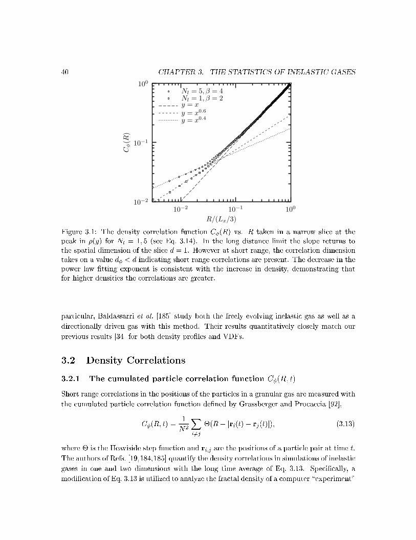
40 CHAPTER 3. THE STATISTICS OF INELASTIC GASESy = x0.4y = x0.6y = xNl = 1, β = 2Nl = 5, β = 4
R/(Lx/3)
Cφ(R
)
10010−110−2
100
10−1
10−2Figure 3.1: The density orrelation fun tion C�(R) vs. R taken in a narrow sli e at thepeak in �(y) for Nl = 1; 5 (see Eq. 3.14). In the long distan e limit the slope returns tothe spatial dimension of the sli e d = 1. However at short range, the orrelation dimensiontakes on a value d� < d indi ating short range orrelations are present. The de rease in thepower law �tting exponent is onsistent with the in rease in density, demonstrating thatfor higher densities the orrelations are greater.parti ular, Baldassarri et al. [185℄ study both the freely evolving inelasti gas as well as adire tionally driven gas with this method. Their results quantitatively losely mat h ourprevious results [34℄ for both density pro�les and VDFs.3.2 Density Correlations3.2.1 The umulated parti le orrelation fun tion C�(R; t)Short range orrelations in the positions of the parti les in a granular gas are measured withthe umulated parti le orrelation fun tion de�ned by Grassberger and Pro a ia [92℄,C�(R; t) = 1N2 Xi6=j �(R� jri(t)� rj(t)j); (3.13)where � is the Heaviside step fun tion and ri;j are the positions of a parti le pair at time t.The authors of Refs. [19,184,185℄ quantify the density orrelations in simulations of inelasti gases in one and two dimensions with the long time average of Eq. 3.13. Spe i� ally, amodi� ation of Eq. 3.13 is utilized to analyze the fra tal density of a omputer \experiment"

3.2. DENSITY CORRELATIONS 41[19℄ designed to mimi Method I, namely,C�;�y(R; t) = 1N�y(N�y � 1) Xi6=j:(ri;rj)2�y�(R� jri(t)� rj(t)j); (3.14)where �y refers to a narrow sli e of width d made a ross the y-dire tion about the peakin �(y), and ri must originate in the middle thirds of �y to a ount for the boundary ondition, that is ri 2 [Lx=3; 2Lx=3℄ and rj 2 [0; Lx℄. The time average of the orrelationfun tion, C�;�y(R) = 1� Z �t=t0 dtC�;�y(R; t) (3.15)is measured in the limit that � � t0. We observe (see Fig. 3.1) that C�;�y(R) demonstratessub-linear s aling for the entire range of �. The existen e of the s aling relation, C�;�y(R) �Rd� allows for a determination of the homogeneity of the parti le positions within �y. Ifd� < d�y, where d�y is the topologi al dimension of the sli e �y, then orrelation betweenthe parti les exist. The results in Fig. 3.1 are for sli es with �yR � 1, therefore d�y = 1.The results demonstrate that short range orrelations exist for all densities. The de reasein the power law �tting exponent is onsistent with the in reased density, demonstratingthat for higher densities the orrelations are greater.3.2.2 The Radial Distribution Fun tion: g(r)As dis ussed in Se . 3.1 the radial distribution fun tion g(r) at onta t (r = d) was utilizedby Chapman and Enskog in their formulation of dense gas kineti theory to a ount for thevolume ex luded by the parti les. That is, as the density of the system is in reased the totalfree spa e allowed for parti le motion is redu ed thus modifying the ollision probability.We ompute g(r) by produ ing a histogram of the distan es between all parti lepairs [8℄. Ea h parti le is translated to the origin and the number of parti les whose enterslie within a ir ular band of area rÆr is measured,g(r) = 1� �Xt=0 1N2 NXi NXj 6=i Æ(r � rij)�rÆr ; (3.16)where � is the total number of time steps averaged over. The existen e of a peak in g(r)at r=d = 1 [see Fig. 3.2(b)℄ for all Nl; � indi ates that stru ture is present. Carnahan andStarling propose a form for the height of the �rst peak in g(r),g(r = d) = 16� 7�16(1 � �)2 ; (3.17)where � is the area fra tion. At low densities, Eq. 3.17 underestimates the measured valueof g(r = d) [see Fig. 3.2 (b)℄. The in rease in the probability for �nding a parti le near it'sneighbor is due to the orrelations in parti le positions due to the parti le inelasti ity.

42 CHAPTER 3. THE STATISTICS OF INELASTIC GASESNl = 5, β = 4.0Nl = 4, β = 4.0Nl = 4, β = 2.0Nl = 3, β = 2.0Nl = 2, β = 2.0Nl = 1, β = 2.0
(a)
r/d
g(r
)
543210
3.5
3
2.5
2
1.5
1
0.5
0
(b)
φ
g(r
=d)
0.60.50.40.30.20.10
4
3.5
3
2.5
2
1.5
1
0.5Figure 3.2: (a) The radial distribution fun tion g(r) vs. r=d for all Nl; � measured in theROI. (b) The value of g(r) at r = d for various densities. The solid line is the proposedform by Carnahan and Starling given in Eq. 3.17 and the dashed line is the Carnahan andStarling form shifted by a onstant value.

3.3. THE MEAN FREE PATH AND TIME 433.3 The Mean Free Path and Time3.3.1 Derivation of The Path Length DistributionPossibly, the most fundamental statisti al measures of a gas of like mole ules is the meanfree path. In 1858 Clausius introdu ed the notion of al ulating the distan e a parti le musttravel before intera ting with another parti le, that in fa t set the stage for the developmentof the kineti theory of gases dis ussed above. If a single spe ies elasti gas of hard spheresin two dimensions is onsidered, then the derivation of the distribution of the mean free pathand subsequently the mean free time is given below. The analysis is based on geometri alarguments that follows the method proposed by Clausius.The \ ollision ylinder" shown in Fig. 3.3 for a hard sphere parti le of diameterd moving through a spatially homogeneous gas of equivalent parti les provides a simplegeometri pi ture of the probability of ollision. First assume that all other parti les arefrozen in spa e and that any parti le who's enter is within the outer ylinder of diameter2d will ollide with the moving parti le. Therefore, area swept out by the moving parti lewill be 2d�v� in unit time, where � is the bidimensional number density2 and �v is the averagevelo ity. However, the initial assumption of a stati assembly is not a omplete physi alpi ture. Therefore, the relative motion of all other parti les must be onsidered. For elasti parti les the average relative speed is rigorously�vr = p2�v: (3.18)The p2 omes from the relative orientation of parti les at onta t, i.e. most ollisionso ur at 90Æ. In the dis ussion of granular materials the proportionality between �vr and �vis a di�erent value, however it will be demonstrated that this will not have any a�e t onthe form of the distribution of path lengths or free times.Knowing the geometry of the ollision ylinder and the system density, the numberof ollisions that a parti le will undergo in unit time is,Z = 2p2 d � �v: (3.19)In order to derive the probability distribution of path lengths P (l) we will need onlythe number of ollisions per unit time Z. As above, onsider a spatially homogeneous olle tion of parti les at a number density �. What we would like is the distan e that aparti le will travel before olliding with another parti le. This is the same as the fra tion ofparti les N=No of a initial No beam of parti les that is being shot into a gas at some timet = 0, that have survived after some time t without undergoing a ollision. The surviving2� is used for dimensional purposes and is simply a dimensional form of the overing fra tion � = NA =(4=3)1=2d� where A is the area of the ontainer and � is as de�ned in Se . 2.4.2.

44 CHAPTER 3. THE STATISTICS OF INELASTIC GASESσ2σ
vFigure 3.3: Collision ylinder produ ed by a parti le moving �v in a unit time. The area ofthe ylinder is �d�v for two dimensions.parti les have traveled a distan e �vt = l. In a time interval dt the number of mole ulesleaving this beam (i.e. those parti les that have ollided) is given by,dN = �NZdt; (3.20)where by integrating over all parti les,Z NNo dNN = �Z Z dt: (3.21)Thus the probability for a parti le to go a distan e l before olliding is,P (l) = NNo = C e�Z t (3.22)= C e�Z l=�v (3.23)= C e�2p2 l d �; (3.24)where C is a normalization onstant determined by R10 dl P (l) = 1. Using Eq. 3.24 thenormalized distribution of path lengths is given by,P (l) = (2p2 d �)e�2p2 d � l: (3.25)Therefore, the mean free path �l is al ulated from the mathemati al de�nition of the meanand the probability given in Eq. 3.25,�l = Z 10 dl l P (l) = 12p2 d �; (3.26)demonstrating that the p2 fa tor introdu ed above for the relative velo ities is only as aling. However, the strong short range orrelations, measured in our experiments (seeSe . 3.2.1), lead to ne essary modi� ations to the form of the distributions of free pathsand times.

3.3. THE MEAN FREE PATH AND TIME 453.3.2 Measured Path Length and Time DistributionsExperimentally, the distribution of paths lengths are measured from the geometri distan ebetween ollision events de�ned in our ROI at ea h Nl; � in the gas regime [see Fig. 3.4(a{f)℄. If Nl � 3, the hoi e of the ROI an have two e�e ts on the measured distribution ofpath lengths. First, if the ROI is hosen su h that the density gradients are large, thenthe variable density will hange the distributions. Se ond, if the ROI is hosen too narrow,then the parti les may not undergo a ollision before leaving. We have tested the resultsfor high Nl to ensure that the measured distributions are not e�e ted by the size of ourROI. As dis ussed in the pre eding paragraphs the distribution of path lengths for an elasti hard-sphere gas (and by a similar treatment the distribution of free times) is given by,P (l) = (2p2 d �) e�2p2 d � l: (3.27)The distribution therefore follows a simple exponential form depending only on the density.However it is lear from the dashed lines in Fig. 3.4(a{f) that the simple form given byEq. 3.27 does not des ribe the behavior over all l. The distributions of times between ollisions P (�) [Fig. 3.5(a{f)℄ is also measured and shows similar behavior to that of thepath length distributions, that is, an overpopulation of the short time bins. This should beexpe ted from the simple relationship between the displa ement and the time.Grossman et al. [93℄ have interpolated the density dependen e of the mean free pathin a granular systems to a ount for higher ollision rates due to in reased short ranged orrelations. Although the interpolation gives a qualitatively a urate orre tion for passingbetween the high and low density limits [see the Se tion below and Fig. 3.6(a)℄, the a tualdistribution of path lengths has not been measured or al ulated in an attempt to a ountfor su h orrelations in granular uids.An empiri al form that well des ribes the measured distributions of path lengths andfree times, P (l) = a (l)�b e� l; (3.28)P (�) = d (�)�e e�f � ; (3.29)where the �tting parameters for the path lengths and free times are shown in Table 3.1for all Nl; �. The proposed forms in Eqs. 3.28{ 3.29 demonstrate a lose �t to the dataover a large range of density. The proposed forms appear to apture both the short l and� power-law behavior. In the dilute ase the form returns to the theoreti al predi tion forlarger path lengths. However, for higher densities the power law behavior extends for themajority of the distribution.

46 CHAPTER 3. THE STATISTICS OF INELASTIC GASESl (cm)
P(l
)10110010−110−2
100
10−1
10−2
10−3
(a)
l (cm)
P(l
)
20151050
100
10−1
10−2
10−3
l (cm)
P(l
)
10110010−110−2
100
10−1
10−2
10−3
10−4
(b)
l (cm)
P(l
)
1614121086420
100
10−1
10−2
10−3
10−4
l (cm)
P(l
)
10110010−110−2
100
10−1
10−2
10−3
10−4
(c)
l (cm)
P(l
)
1086420
100
10−1
10−2
10−3
10−4
10−5
l (cm)
P(l
)
10110010−110−2
100
10−1
10−2
10−3
10−4
(d)
l (cm)
P(l
)
6543210
100
10−1
10−2
10−3
10−4
10−5
l (cm)
P(l
)
10010−1
100
10−1
10−2
10−3
10−4
(e)
l (cm)
P(l
)
21.510.50
100
10−1
10−2
10−3
10−4
10−5
l (cm)
P(l
)
10010−1
100
10−1
10−2
10−3
10−4
(f)
l (cm)
P(l
)
21.510.50
100
10−1
10−2
10−3
10−4
10−5Figure 3.4: The probability distributions of path lengths P (l) vs. l, on a log-linear s ale,and inset log-log s ale (a) Nl = 1 ; � = 2:0, (b) Nl = 2 ; � = 2:0, ( ) Nl = 3 ; � = 2:0,(d) Nl = 4 ; � = 2:0, (e) Nl = 4 ; � = 4:0, (f) Nl = 5 ; � = 4:0. The dashed line showsthe theoreti al form given by Eq. 3.27 derived for elasti parti les, and the solid line is anempiri al �t given by Eq. 3.28. Table 3.1 shows the �t parameters.

3.3. THE MEAN FREE PATH AND TIME 47τ (s)
P(τ
)10010−110−2
100
10−1
10−2
10−3
(a)
τ (s)
P(τ
)
1.41.210.80.60.40.20
100
10−1
10−2
10−3
τ (s)
P(τ
)
10010−110−2
100
10−1
10−2
10−3
(b)
τ (s)
P(τ
)
1.210.80.60.40.20
100
10−1
10−2
10−3
τ (s)
P(τ
)
10−110−2
100
10−1
10−2
10−3
10−4
(c)
τ (s)
P(τ
)
0.60.50.40.30.20.10
100
10−1
10−2
10−3
10−4
10−5
τ (s)
P(τ
)
10−110−2
100
10−1
10−2
10−3
10−4
(d)
τ (s)
P(τ
)
0.40.350.30.250.20.150.10.050
100
10−1
10−2
10−3
10−4
10−5
τ (s)
P(τ
)
10−110−2
100
10−1
10−2
10−3
10−4
(e)
τ (s)
P(τ
)
0.30.250.20.150.10.050
100
10−1
10−2
10−3
10−4
10−5
τ (s)
P(τ
)
10−110−2
100
10−1
10−2
10−3
10−4
(f)
τ (s)
P(τ
)
0.250.20.150.10.050
100
10−1
10−2
10−3
10−4
10−5Figure 3.5: The probability distributions of free times P (�) vs. � , on a log-linear s ale(a) Nl = 1 ; � = 2:0, (b) Nl = 2 ; � = 2:0, ( ) Nl = 3 ; � = 2:0, (d) Nl = 4 ; � = 2:0, (e)Nl = 4 ; � = 4:0, (f) Nl = 5 ; � = 4:0. The solid line is a �t given by Eq. 3.29.

48 CHAPTER 3. THE STATISTICS OF INELASTIC GASESNl � a b 1 2 0.031 0.428 0.1542 2 0.025 0.603 0.3933 2 0.008 0.932 0.7424 2 0.003 1.258 1.4894 4 0.002 0.970 3.1715 4 0.002 1.096 2.887Nl � d e f1 2 0.0027 0.511 2.9692 2 0.0025 0.665 6.0243 2 0.0003 1.203 8.3064 2 0.0008 1.209 16.914 4 0.0002 1.043 26.455 4 0.0005 1.384 28.33Table 3.1: Fitting parameters for Eqs. 3.28, 3.29. The values are arranged su h that thevalues in the top half orrespond to P (l), and the bottom half for P (�).3.3.3 The Mean Free Path and Average SpeedFrom the distribution of path lengths and free times, the mean free path and time are al ulated by utilizing the �tting form and the parameters given in Table 3.1. Figure 3.6(a)demonstrates the two theoreti al forms of the mean free path. The solid line in the �gureis the kineti theory result Eq. 3.26, and the dashed line is the interpolated form derivedby Grossman et al.The ratio of the mean free path to the mean ollision time should determine theaverage speed �v in the ROI where the distributions are measured. We have taken the ratiosof the integrated distributions, �v = �l�� = R10 l P (l) dlR10 �P (�) d� ; (3.30)and ompared that to the average of the speed distribution hvx;yi in the same ROI. In Fig. 3.6both measurements of the average speed are shown for all Nl; �. The agreement is within10% over the entire range of Nl; � indi ating that the proposed forms in Eqs. 3.28,3.29quantitatively apture the behavior of the distributions.It is noteworthy to mention the instantaneous speed, or the ratio of the path length tothe free time, vinst = l=� vs. l, the path length. The ratio is found not to be a onstant overall values of l, implying that the average speed of the system depends on the distan e or timebetween ollisions (see Fig. 3.7). Spe i� ally it implies that when parti les are within a few
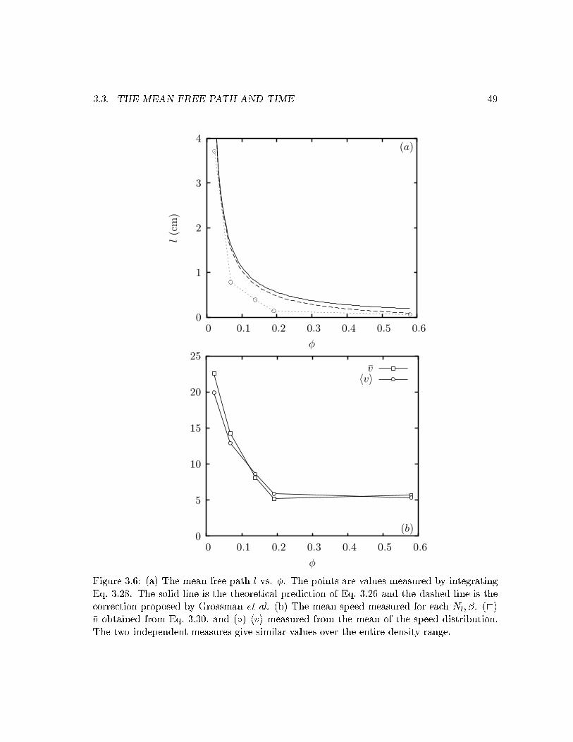
3.3. THE MEAN FREE PATH AND TIME 49(a)
φ
l(c
m)
0.60.50.40.30.20.10
4
3
2
1
0
〈v〉v̄
(b)
φ
0.60.50.40.30.20.10
25
20
15
10
5
0Figure 3.6: (a) The mean free path l vs. �. The points are values measured by integratingEq. 3.28. The solid line is the theoreti al predi tion of Eq. 3.26 and the dashed line is the orre tion proposed by Grossman et al. (b) The mean speed measured for ea h Nl; �. (2)�v obtained from Eq. 3.30, and (Æ) hvi measured from the mean of the speed distribution.The two independent measures give similar values over the entire density range.

50 CHAPTER 3. THE STATISTICS OF INELASTIC GASESNl = 2Nl = 1
l(cm)
v inst=
l/τ
(cm
s−1)
20151050
40
35
30
25
20
15
10
5
0Figure 3.7: The ratio of the path length and the free time vinst = l=� vs. l for Nl = 1; 2. Thisplot learly demonstrates that the velo ity is strongly dependent on the distan e betweenparti les. The dashed lines show the average velo ity for the values of Nl. For an elasti gas vinst should have a onstant value for all l.parti le diameters, their instantaneous velo ity has a value well below mean. In an elasti gas, vinst should have a onstant value determined by the distribution of parti le velo ities. Adistan e dependent instantaneous vinst again demonstrates the inherent orrelation manifestin dissipative gas systems.3.4 The Distribution of Parti le Velo itiesThe distribution of the x- and y- omponents of the parti le velo ities are plotted in Figs. 3.8{3.10. The distributions orrespond to velo ities that are measured within a narrow region ofinterest (ROI). The ROI is de�ned by making a sli e a ross the y-dire tion that is enteredupon the peak in �(y) with and extent of �10% of the peak in �(y) [see Fig. 2.3(b)℄ whileex luding parti les lying within a distan e of 3d from the side walls. We utilize this ROI toensure that large gradients in �(y), and the lustering produ ed by the side-walls, do nota�e t the measured VDFs. Ea h distribution orrespond to � 2�106 unique velo ities thatare found within our ROI.The velo ities of parti les that omprise a lassi al elasti or ideal gas follow a distri-bution given by the Maxwell-Boltzmann formP (v) = (2�kBT )�d=2e�v2=2kBT (3.31)

3.4. THE DISTRIBUTION OF PARTICLE VELOCITIES 51(a)
vx (cm s−1)
P(v
x)
3020100-10-20-30
0.03
0.02
0.01
0
(b)
vx (cm s−1)
P(v
x)
3020100-10-20-30
0.04
0.03
0.02
0.01
0
(c)
vx (cm s−1)
P(v
x)
3020100-10-20-30
0.06
0.05
0.04
0.03
0.02
0.01
0
(d)
vx (cm s−1)
P(v
x)
3020100-10-20-30
0.08
0.06
0.04
0.02
0
(d)
vx (cm s−1)
P(v
x)
3020100-10-20-30
0.05
0.04
0.03
0.02
0.01
0
(f)
vx (cm s−1)
P(v
x)
3020100-10-20-30
0.08
0.06
0.04
0.02
0Figure 3.8: The velo ity distribution fun tions P (vx) vs. vx on a linear-linear s ale. (a)Nl = 1 ; � = 2:0, (b) Nl = 2 ; � = 2:0, ( ) Nl = 3 ; � = 2:0, (d) Nl = 4 ; � = 2:0, (e)Nl = 4 ; � = 4:0, (f) Nl = 5 ; � = 4:0. The solid urves are a least squares �t to a Gaussianform given by Eq. 3.31. Note that the deviation from a Gaussian distribution extends allthe way to the lowest velo ity bins. Ea h distribution orrespond to � 2 � 106 uniquevelo ities that are found within the ROI de�ned in the text.

52 CHAPTER 3. THE STATISTICS OF INELASTIC GASESwhere, d is the dimensionality of the system, kB is Boltzmann's onstant, and T is thetemperature of the heat bath that the system is in onta t with. Hen e, if a system ofparti les is at equilibrium, its temperature determined by the width of the distribution ofparti le velo ities. Equation 3.31 is �t to the data for the x- omponents of the velo ities,and is shown on both linear and logarithmi s ales [Fig. 3.8,3.9℄. We observe that the formgiven by Eq. 3.31 displays deviations both at low and high velo ities. The distributions ofvelo ities are normally displayed in a log-linear fashion to a entuate the tails of the VDF,however this suppresses the deviations at low velo ities. By plotting the distributions on alinear s ale we display the more statisti ally signi� ant deviations from Eq. 3.31.In a re ent experimental work [192℄, a two-dimensional olle tion of parti les is driveninto a steady state (usingMethod I with � = 90o). Using analysis te hniques that are similarto those des ribed in Chapter 2, the authors proposed a governing form for the VDF givenby R(vx) = Ae�B jvx=Txj�1:5 ; (3.32)where A and B are onstants and Tx is the x- omponent of the granular temperatureTx;y = 12(hv2xi+ hv2yi): (3.33)The authors laim to observe a universal VDF that is parameterized by a single value,regardless of the system density or the value of the inelasti ity of the parti les. Fromour VDFs, whose orresponding densities range over an order of magnitude and where theaverage inelasti ity varies by nearly a fa tor of two, we annot �nd any single parameter �tthat des ribes the overall form.The VDFs for the y omponents, P (vy) vs. vy for ea h Nl � in our ROI are alsomeasured, [see Fig. 3.10(a{f)℄ and are highly skewed by the asymmetry in the drivingagainst the dire tion of gravity.To identify the e�e ts that the asymmetry in P (vy) has upon P (vx), we have separatedthe vx distributions by the sign of vy, i.e. P (vxj + vy;�vy). The onditional distributionsfor Nl = 1; � = 2 and Nl = 5; � = 4 are plotted in Fig. 3.11(a,b) respe tively. Thevelo ities have been res aled by pTx so in order to demonstrate the simple s aling for ea hdistribution. The ratio of the separated granular temperatures,� = T(xj+vy)T(xj�vy) (3.34)is plotted over all Nl; � in Fig. 3.11. The dashed line is a �t whi h shows that for all densitythe temperature is � 40% greater in dire tion of the driving wall as to that of the returningparti les.Figures 3.9,3.10(a{f) show that the distributions for ea h are highly non Gaussian.However, at low Nl the distributions of the vy omponents follow a form that is the mixture

3.4. THE DISTRIBUTION OF PARTICLE VELOCITIES 53(a)
vx (cm s−1)
P(v
x)
6040200-20-40-60
10−1
10−2
10−3
10−4
10−5
10−6
(b)
vx (cm s−1)
P(v
x)
6040200-20-40-60
10−1
10−2
10−3
10−4
10−5
10−6
(c)
vx (cm s−1)
P(v
x)
6040200-20-40-60
10−1
10−2
10−3
10−4
10−5
10−6
(d)
vx (cm s−1)
P(v
x)
6040200-20-40-60
10−1
10−2
10−3
10−4
10−5
10−6
(e)
vx (cm s−1)
P(v
x)
6040200-20-40-60
10−1
10−2
10−3
10−4
10−5
10−6
(f)
vx (cm s−1)
P(v
x)
6040200-20-40-60
10−1
10−2
10−3
10−4
10−5
10−6Figure 3.9: The velo ity distribution fun tions P (vx) vs. vx on a log-linear s ale.(a) Nl =1 ; � = 2:0, (b) Nl = 2 ; � = 2:0, ( ) Nl = 3 ; � = 2:0, (d) Nl = 4 ; � = 2:0, (e) Nl = 4 ; � =4:0, (f) Nl = 5 ; � = 4:0. The solid urves are a least squares �t to a Gaussian form given byEq. 3.31. Here the apparent deviation in the tails of the distribution fun tions are present.

54 CHAPTER 3. THE STATISTICS OF INELASTIC GASES(a)
vy (cm s−1)
P(v
y)
6040200-20-40-60-80-100
10−1
10−2
10−3
10−4
10−5
10−6
(b)
vy (cm s−1)
P(v
y)
6040200-20-40-60-80-100
10−1
10−2
10−3
10−4
10−5
10−6
(c)
vy (cm s−1)
P(v
y)
6040200-20-40-60-80-100
10−1
10−2
10−3
10−4
10−5
10−6
(d)
vy (cm s−1)
P(v
y)
6040200-20-40-60-80-100
10−1
10−2
10−3
10−4
10−5
10−6
(e)
vy (cm s−1)
P(v
y)
6040200-20-40-60-80-100
10−1
10−2
10−3
10−4
10−5
10−6
(f)
vy (cm s−1)
P(v
y)
6040200-20-40-60-80-100
10−1
10−2
10−3
10−4
10−5
10−6Figure 3.10: The velo ity distribution fun tions P (vy) vs. vy on a log-linear s ale.(a)Nl = 1 ; � = 2:0, (b) Nl = 2 ; � = 2:0, ( ) Nl = 3 ; � = 2:0, (d) Nl = 4 ; � = 2:0, (e)Nl = 4 ; � = 4:0, (f) Nl = 5 ; � = 4:0. The large skewness in the distributions for thenegative values of vy is due primarily to the driving from the bottom wall. Parti les thatare moving in the �y dire tion are leaving the moving wall. The dashed lines in (a) areindependent Gaussian �ts.

3.4. THE DISTRIBUTION OF PARTICLE VELOCITIES 55−vy
+vy (a)
vx/√
Tx
√T
xP
(vx)
86420-2-4-6-8
100
10−1
10−2
10−3
10−4
10−5
−vy
+vy (b)
vx/√
Tx
√T
xP
(vx)
1050-5-10
100
10−1
10−2
10−3
10−4
10−5Figure 3.11: The onditional distributions of velo ities P (vxj+vy;�vy) s aled byp(Tx) vs.vx normalized byp(Tx). (a) Nl = 1 and (b) Nl = 5. The simple s aling by the temperaturefor ea h onditional distribution indi ates a universality for ea h Nl.

56 CHAPTER 3. THE STATISTICS OF INELASTIC GASESy = 0.58 (c)
φ
ζ
0.60.50.40.30.20.10
1
0.8
0.6
0.4
0.2Figure 3.12: The ratio of the granular temperatures � = T(xj+vy)T(xj�vy) . Over a broad range indensity the ratio is losely �t by a onstant value � = 0:58, indi ating that the temperaturein the dire tion of driving is nearly 40% greater than the return temperature.of two distin t Gaussians [see 3.10(a)℄. As the density, and hen e the ollision frequen y(see Se . 3.8), is in reased, the two Gaussians be ome less distin t and P (vy) be omes askewed distribution with a peak at vy = 0. We therefore on lude that in fa t the ollisionpro ess is leading to the non-Gaussian forms of the x- omponent distributions based on theform of P (vy). That is, for the lowest density, Nl = 1, the parti les have two thermalizingpro esses that determines the form of the vy omponent distributions:� First, the left side of the distribution in Fig 3.10(a) is e�e tively the Gaussian due toparti les moving away from the driving wall after being heated.� Se ond, the right side is the Gaussian due to the in uen e of the top wall and gravitythat returns the parti les ba k to the bottom wall.The pro esses des ribed assumes that the driving wall is imparting random velo ities whosesignature is a Gaussian distribution of velo ities.3 The perpendi ular omponents of theparti le velo ities shown in Fig 3.10(a) are plotted in Figs. 3.9(a){3.11(a). The P (vx)distributions are also omprised of two types of velo ities. First, there exist ontributionsfrom parti les leaving the driving wall that dire tly re e t the in oming vx prior to a3We observe that this is not parti ularly the ase; in fa t parti les require at least one ollision in orderfor the distribution of their velo ities to assume a Gaussian.

3.4. THE DISTRIBUTION OF PARTICLE VELOCITIES 57 ollision. Se ond, are the parti les whose velo ities are distributed due to ollisions withother parti les. It is reasonable to assume that the �rst ontribution to the distributionshould small for Nl = 1 and a tually should be more Gaussian due to the strong ouplingbetween the x and y omponents. We on lude that the non-Gaussian form of P (vx) is notdue to the dire t in uen e of the driving, but is a dire t onsequen e of the inter-parti le ollision pro ess.3.4.1 S aling Properties and UniversalityThe distributions of the velo ity omponents perpendi ular to the driving dire tion areshown to simply s ale when they are preferentially dis riminated by the sign of their velo ityin the y-dire tion at a parti ular density. However, su h a s aling relationship does notimmediately appear to exist for di�erent densities. Figure 3.13(a,b) shows the velo itiesnormalized bypTx for allNl; � on both log-lin and log-log s ales respe tively. It is lear fromFig. 3.13(a), that as the density in reases the distributions be ome highly non-Gaussian [34℄.In parti ular, Fig. 3.13(b) demonstrates that there does not appear to be an underlyinguniversal exponent that well �ts the distribution fun tion.We do indeed observe that a universal power-law with an exponential uto� apturesthe tails of the distribution fun tion. In Fig. 3.14 the distribution fun tions plotted ona logarithmi s ale and are arbitrarily shifted to demonstrate the possible universality inthe tails. However, the noise is large, therefore making a de�nitive statement about theexisten e of universal tails diÆ ult. The distributions an be des ribed as having threeunique regimes and are universal over two of those regimes. The form of the distributionsfor P (�vx ! 0) are not universal. Away from the peak, P (vx) shows two spe i� points ofslope hange or knees. Between the �rst and se ond knee, the power law that well des ribesall of the distributions is P (vx) � v�3:0x . After the se ond knee the power law is ut-o� bya rapid exponential de ay (see Fig. 3.14).S aling with yThe x- omponent of the granular temperature Tx (see Eq. 3.33), is measured as a fun tionof distan e from the driving wall to probe the s aling behavior of the velo ity distributionsas a fun tion of the distan e from the energy sour e. Figure 3.15(a) shows Tx vs. y for allNl and �. At low densities (Nl � 2), Tx(y) initially in reases and then de ays. In ontrast,for (Nl � 3), Tx(y) has a distin t minimum. We note that Tx(y) never rea hes a onstantvalue and the minimum (maximum) does not orrespond to the peak in �(y).To further show the non-universality of the distribution of parti le velo ities thekurtosis x = hv4xihv2xi2 ; (3.35)

58 CHAPTER 3. THE STATISTICS OF INELASTIC GASES(a)
vx/√
Tx
√T
xP
(vx)
1050-5-10
100
10−1
10−2
10−3
10−4
10−5
Nl = 5, β = 4Nl = 4, β = 4Nl = 4, β = 2Nl = 3, β = 2Nl = 2, β = 2Nl = 1, β = 2
(b)
vx/√
Tx
√T
xP
(vx)
1010.1
100
10−1
10−2
10−3
10−4
10−5Figure 3.13: The res aled distributions pTxP (vx) vs. vx=pTx. (a) The res aled distribu-tions on a log-linear s ale that demonstrate that a simple s aling by the granular temper-ature does not ollapse the distributions on a universal form. (b) The same as (a) plottedon a log-log s ale to demonstrate that a simple power law does also does not des ribe thedistributions. We not that a stret hed exponential only �ts the Nl = 1; � = 2 data with apower of 1.5.

3.5. SPATIAL CORRELATION OF PARTICLE VELOCITIES 59
y = ex/0.4y = −3.0xNl = 5, β = 4.0Nl = 4, β = 2.0Nl = 3, β = 2.0Nl = 2, β = 2.0Nl = 1, β = 2.0
log vx
log
P(v
x)
1.00.90.80.70.60.50.40.3
-1.0
-2.0
-3.0
-4.0
-5.0
-6.0Figure 3.14: The res aled distributions P (vx) vs. vx res aled to demonstrate the possibles aling of the distribution tails. The data has been arbitrarily shifted to demonstrate thepossible s aling of the tails. The power-law de ay of the distribution fun tion is followedby an exponential ut-o�.is measured as a fun tion of distan e from the driving wall. If the velo ity distribution isa Gaussian then = 3, and if the distribution is given by Eq. 3.32 then = 3:576, shownby the dashed line in Fig. 3.15. The measured values for are found to greatly ex eedthe value for a Gaussian and also vary as a fun tion of distan e from the driving. Thisanalysis is onsistent with our previous results [34℄ and re ent MD simulations of Brey andRuiz-Montero [40℄ that losely mimi our experiments.3.5 Spatial Correlation of Parti le Velo itiesAs dis ussed in Se . 3.1 Maxwell's fundamental, leading to his proof of the distribution ofparti le velo ities was somewhat awed in it's primary assumption. Maxwell stated:...F (u)du is the probability that a mole ule should possess an x- omponent ofthe velo ity between u and u+ du, and that F (u) is independent of v; w....Now in a gas at rest there is nothing to distinguish on dire tion from another;thus f(u; v; w) an depend on u; v; w only through the invariant u2 + v2 + w2.Thus n F (u) F (v) F (w) = f(u; v; w) = �(u2 + v2 + w2);

60 CHAPTER 3. THE STATISTICS OF INELASTIC GASES(a)
y(cm)
Tx(y
)
121086420
120
100
80
60
40
20
Nl = 5, β = 4Nl = 4, β = 4Nl = 4, β = 2Nl = 3, β = 2Nl = 2, β = 2Nl = 1, β = 2(b)
y(cm)
γx(y
)
121086420
12
11
10
9
8
7
6
5
4
3Figure 3.15: (a) The granular temperature Tx = hv2xi as a fun tion of y, the distan efrom the driving wall for ea h Nl; �. If the isothermal atmosphere ondition was satis�edthese would be onstant values for all y above the peak in �(y). For values of Nl > 2 thetemperatures follow a non-monotoni form that has a distin t minimum. (b) The kurtosis, x measured from P (vx) as a fun tion of the distan e from the driving. The values given bya Gaussian (solid line) and the form proposed in Eq. 3.32 (dashed) are only attained veryfar from the energy sour e.

3.5. SPATIAL CORRELATION OF PARTICLE VELOCITIES 61say. The solution of this fun tional equation is given byF (u) = XeY u2f(u; v; w) = �(u2 + v2 + w2) = n X3 eY (u2+v2+w2)::::The parti ular aw is the assumption that the omponent distributions and hen e the velo -ities themselves are not orrelated in any way. It widely known that the kineti des riptionof elasti gases must take into a ount orrelations between velo ities due to e�e ts su has ex luded volume. It is therefore not implausible that su h orrelations should exist, andpossibly be a entuated in granular gases.The overall e�e t of dissipation is well demonstrated by freely evolving granular uidsby the appearan e of vorti ular regions and the build up of long range spatial orrelationsin the velo ities [86, 95, 148, 149℄. Bizon demonstrated that for driven systems, where thedriving an is either dire ted or noise based, the regions of vorti ity and long range spatial orrelations exist [26, 155℄.In Ref. [34℄ we demonstrated the existen e of long range velo ity orrelations for awide range of densities by measuring the osines of the angles between velo ities of parti lesas a fun tion of their separation.4 Here, in keeping with the methods of Bizon, we mea-sure the orrelations proje ted onto the ve tor onne ting the parti les and the omponentperpendi ular to it given by, Cv(r)jj;? = 1N NXi6=j vjj;?i vjj;?j ; (3.36)where N is the number of parti le pairs, subs ripts i and j denote parti les separatedby a distan e r, and vjj, v? are the parallel and perpendi ular omponents respe tively.Figure 3.16(a) shows Cv(r)jj as a fun tion of r=d, s aled by the granular temperature.Figures 3.16(a,b) demonstrate that at very short distan es their is a rapid exponentialde ay, followed by a long ranged power-law form. Moon et al. [155℄ �nd similar results forevent driven hard sphere mole ular dynami s simulations.4In Chapter 4 this te hnique will be extended to quantify surfa e waves in a two-dimensional granularliquid.

62 CHAPTER 3. THE STATISTICS OF INELASTIC GASESNl = 5, β = 4Nl = 4, β = 4Nl = 4, β = 2Nl = 3, β = 2Nl = 2, β = 2Nl = 1, β = 2(a)
r/σ
Cv;||
1086420
0.2
0.16
0.12
0.08
0.04
0
(b)
r/σ
Cv;⊥
1086420
0.06
0.04
0.02
0Figure 3.16: (a) The parallel omponents of the spatial velo ity orrelation fun tion, Cv(r)jjas a fun tion of r=d s aled by the granular temperature Tg. (b) The s aled perpendi ular omponents of the spatial velo ity orrelation fun tion Cv(r)?

3.6. SELF DIFFUSION 633.6 Self Di�usionThe Mean Square Displa ementThe mean square displa ement of the x- omponent of the parti le positions is measuredover long times from the parti le traje tories [8℄,Cx2 = hjx(t)� x(0)j2i = 1NpNstmax Np;NsXi;j=0 tmaxX�t=1 jxij(to)� xij(to +�t)j2: (3.37)where Ns is the total number of data sets, Np is the number of parti les and tmax is thetotal number of time origins.The long time form of Cx2 for ea h Nl; � [Fig. 3.17(a)℄ is linear indi ating di�usivemotion. For short times, the parti les experien e ballisti motion given by the relationh�x2i = hvi2t2, indi ated by the dashed line in Fig. 3.17(b). The arrows in Fig. 3.17(b)indi ate the value of the ollision time � derived dire tly from the distribution of free times(see Se . 3.3.2). The independently measured ollision time demonstrates the time that theballisti regime rosses over to the di�usive regime as is expe ted. As Nl is in reased, therange of the ballisti regime dramati ally de reases indi ating a de rease in the ollisiontime � . The ballisti and di�usive regimes are onsistent with what is expe ted for kineti theory of elasti , �nite-sized parti les.The velo ity auto orrelation fun tionThe velo ity auto orrelation fun tion (VAF) is omputed for the x omponents of thevelo ities [8℄ Cv(t) = 1NpNstmax Np;NsXi;j=0 tmaxX�t=1 vij(to) � vij(to +�t); (3.38)where Ns is the total number of data sets, Np is the number of parti les and tmax is the totalnumber of time origins. In Fig. 3.18, shows the measured values of the VAF normalized byhv20i are plotted versus t in se onds.In simulations of hard sphere uids, Alder and Wainwright [7℄ �rst found that theform for the VAF was strongly depended on the density of the system. For very low densitiesthe hara teristi form of the orrelation fun tion was given simply byCv(t) = hv20ie�t=� ; (3.39)where � is the ollision time. If the density of the system is in reased however, the formof Eq. 3.39 breaks down and Cv(t) an be ome negative with long range tails due to the aging of parti les by their neighbors. We �nd that the lowest density ase be omes neg-atively orrelated and remains so after the de ay from hv20i (Fig 3.18). We explain this

64 CHAPTER 3. THE STATISTICS OF INELASTIC GASES(a)
t (s)
Cx2
21.510.50
40
30
20
10
0
y = x2Nl = 5, β = 4Nl = 2, β = 2
(b)
τ = 0.055
τ = 0.011
t (s)
Cx2
10010−110−2
102
101
100
10−1
10−2
10−3Figure 3.17: (a) The mean square displa ement Cx2 vs. t for all Nl; �, there is a distin tdi�usive regime for long times. (b) Cx2 for (Æ) Nl = 2; � = 2 and (D) Nl = 5; � = 4. Thedashed line has a slope of two, indi ating a ballisti regime that rosses over ontinuously tothe di�usive regime. The arrows indi ate the value of the mean free time for the Nl shown, al ulated from the integral of Eq. 3.29 demonstrating a onsisten y for the time that theparti les begin to undergo ollisions.

3.6. SELF DIFFUSION 65Nl = 5, β = 4Nl = 4, β = 4Nl = 4, β = 4Nl = 3, β = 2Nl = 2, β = 2Nl = 1, β = 2
t (sec)
Cv
1.20.80.40
1
0.8
0.6
0.4
0.2
0
-0.2Figure 3.18: The velo ity auto orrelation fun tion Cv vs. t normalized by hv20i for all Nl; �.apparent ontradi tion with Ref. [7℄ as a �nite size e�e t. That is, the parti les are inter-a ting frequently with the side-walls that oppose the driving dire tion at low densities, thusreversing the sign of velo ity ve tors, thus leading to the observed anti- orrelation. Thepredominan e of the sidewall intera tions are s reened for the higher densities due to thein reased number of parti le-parti le ollisions, therefore no anti- orrelations are observed.Self Di�usionThe self di�usion onstantDs, an be al ulated for a system of parti les by either evaluatingthe time integral of the velo ity auto orrelation fun tion,Ds = Z 10 Cv(t)dt; (3.40)or using the relationship between the mean square displa ement of the parti les and timeover long times, Ds = limt!1 12 d tCx2(t); (3.41)where d is spatial dimension. From kineti theory [97℄, the di�usion onstant of a two-dimensional gas is, Ds = d8�g(d) ��Tm �1=2 ; (3.42)

66 CHAPTER 3. THE STATISTICS OF INELASTIC GASESDv
Dx2
φ
self
diff
usi
on
(cm
s1)2
0.60.50.40.30.20.10
25
20
15
10
5
0Figure 3.19: The di�usion onstants al ulated for ea h �, where (O) orresponds to thenumeri al integration of Cv from Fig. 3.18, and (2) orresponds to the least squares �t ofCx2 from Fig. 3.17. The dashed line shows the kineti theory result for a �xed temperature,that is given by the average measured value over this range of �.where g(d) is the radial orrelation fun tion at onta t [99℄ given by the Carhnahan andStarling form (see Se . 3.2.2).By numeri ally integrating the urves in Fig. 3.18, and performing a least squares �tto the data in Fig. 3.17(a) after the ballisti regime, we obtain the self-di�usion onstant[see Fig. 3.19℄. We �nd that the values for the self-di�usion from Eqs. 3.40 and 3.41 areself onsistent. The solid line in Fig. 3.19 shows the form of Eq. 3.42 with the temperatureT given by the granular temperature. The onstants in Eq. 3.42 are determined fromsystem parameters. The theory for the di�usion of elasti parti les, given by Eq. 3.42 losely mat hes our results for all �. Thus we show that the e�e ts of inelasti ity on theself-di�usion are small.3.7 The Equation of State and Hydrodynami sEn ouraged by the su ess of the previous se tion, where the self di�usion onstant demon-strated a onsisten y with the simpli�ed predi tions of kineti theory, we now attempt toextend our analysis to a hydrodynami interpretation.The fundamental assumption of hydrodynami s is that global modes are long-wavelengthand slowly varying ompared to the dynami s of the onstituent parti les (i.e. long time av-erages suppress u tuations at the parti le level) [53℄. The question that arises for granular

3.7. THE EQUATION OF STATE AND HYDRODYNAMICS 67Nl = 1, β = 2Nl = 1, β = 2Nl = 1, β = 2Nl = 1, β = 2Nl = 1, β = 2Nl = 1, β = 2(b)
y (cm)
g(ρ
,y)
1614121086420
2.4
2.2
2.0
1.8
1.6
1.4
1.2
1.0Figure 3.20: The radial orrelation fun tion at onta t g(d; y) given by the Carhnahan andStarling form (Eq. 3.17) vs. y, the distan e from the driving wall for all Nl; �.hydrodynami s, (viz. are we at liberty to assume that ows in our system are perturbationsabout thermodynami equilibrium) is one that must be tested experimentally. The hydro-dynami equations5 for granular materials have been developed through the kineti theoryformalisms [26,114℄. The main distin tion between the hydrodynami s of normal uids andgranular uids is the form of the onstitutive relations and the existen e of a sink term thata ounts for the loss of energy through inelasti ollisions that is added to Eq. 3.6.The equation of state for dilute gases relates the pressure to the temperature and thedensity through the standard form, P = �T: (3.43)For the following analysis the temperature and density will all be the averages of the valuesin the y-dire tion; taken, as before, in narrow sli es along the y-dire tion and averaged alongthe x-dire tion to form pro�les. For dilute gases, the transport of heat and mass simplydepends on kineti s (i.e. transport through momentum ex hange due to ollisions is not onsidered) and Eq. 3.43 should be valid. As demonstrated in Se . 2.4.2 the density for ourexperiments varies non-monotoni ally as a fun tion of distan e from the driving wall [seeFig. 2.3(b)℄. As dis ussed gradients must exist in all experiments on granular gases dueto the asymmetry driving w. r. t. gravity and we must expe t that these gradients makea simplisti equation of state an (Eq. 3.43) in omplete des ription. Therefore, two fa tors5A losed set of equations for a redu ed number of �elds that des ribe uid phenomenon.

68 CHAPTER 3. THE STATISTICS OF INELASTIC GASES
(a)
y (cm)
Ty
(cm
s−1)2
1614121086420
500
400
300
200
100
0
Nl = 5, β = 4Nl = 4, β = 4Nl = 4, β = 2Nl = 3, β = 2Nl = 2, β = 2Nl = 1, β = 2
(b)
y (cm)
dT
y/dy
1614121086420
40
20
0
-20
-40
-60
-80
-100
-120
-140
-160Figure 3.21: (a) The granular temperature in the y-dire tion Ty vs y. The temperatureundergoes an inversion for all Nl; � ex ept Nl = 1. The solid line is a linear �t to the regionfollowing the minimum for Nl = 3; � = 2. (b) The gradient of the temperature rTy vs. y.

3.7. THE EQUATION OF STATE AND HYDRODYNAMICS 69
y (cm)
Ty
ρ(y
)
120
100
80
60
40
201086420
0.30
0.25
0.20
0.15
0.10
0.05
0.00Figure 3.22: The density �(y) and the temperature Ty vs. y for Nl = 4; � = 2. Notethat the minimum in the temperature (dashed verti al line) does not orrespond to themaximum in the density (solid verti al line).must be onsidered, the possibility of higher order orre tions due to ollisional transfer andex luded volume, and that orre tion must be position dependent to a ount for the densitygradient. The form of the high density equation of state is derived via a viral expansionabout the density and to se ond order takes the approximate formP = �T (1 + �G); (3.44)where G = �g(d), � = (1 + �), and g(d) is the value of the radial distribution fun tionat onta t (see Se . 3.2.2). Carnahan and Starling [45℄ proposed a popular model for the orre tion due to short range orrelations given by Eq. 3.17, that in the limit of low densityreturns g(d) ! 1. The measured value of g(d; y) as a fun tion of the distan e from thedriving wall is shown in Fig. 3.20. Due to the existen e of the gradients in the density adire t omparison to the height of the �rst peak in g(r) measured dire tly from parti lepositions not straight forward. However, the two values are onsistent to within 15% whenmeasured in the same region.As dis ussed in Se . 3.4.1, the x- omponent of the temperature, Tx, has a non-monotoni dependen e on the distan e from the driving wall. Similarly, the y omponent ofthe temperature, Ty, displays the same distin t minimum followed by a linear in rease. InFig. 3.21(a) the temperature pro�les are plotted as a fun tion of distan e from the drivingwall and demonstrate the sharp negative gradient to a minimum that is then followed bya linear in rease of the temperature as a fun tion of distan e from the driving wall. We

70 CHAPTER 3. THE STATISTICS OF INELASTIC GASES
φ
∇y
T
0.60.50.40.30.20.10
14
12
10
8
6
4
2
0
-2
-4Figure 3.23: The slopes of the temperature gradient ryTy versus the density � taken byleast squares �ts to the data in Fig. 3.21(a) above the minimum. The negative values forthe lowest density is due to the �nite extent to whi h the parti les travel before intera tingwith the upper boundary.observe that the numeri al derivative of the temperature [Fig. 3.21(b)℄ re e ts the sharpde rease in temperature followed by a plateau to a onstant value. In Fig. 3.22 the valuesof both � and Ty for Nl = 4; � = 2 are shown together to demonstrate that the minimumof the temperature pro�le does not dire tly oin ide with the maximum of the density. Asthe density is in reased the slope of the temperature in rease to a saturation value (seeFig. 3.23). However, due to the upper boundary, the lowest density Nl = 1; � = 2 neverrea hes a temperature minimum indi ated by the negative value of it's slope. UtilizingEq. 3.44 and the results for the pro�les of �, Ty, and G(�) we al ulate the pressure as afun tion of y (see Fig. 3.24). Surprisingly, we �nd that the pressure is also a non-monotoni fun tion of y. Close to the driving wall, the pressure in reases to a peak and then de ays asexpe ted for a gas in the presen e of gravity. Momentum balan e implies that the pressuremust obey the barometri law d(�Ty)dy = ��g; (3.45)where g is the a eleration of gravity. Due to the non-vanishing gradient of temperaturethe general form of the pressure gradient must be taken into a ountTy d�dy + �dTydy = ��g: (3.46)

3.7. THE EQUATION OF STATE AND HYDRODYNAMICS 71Nl = 5, β = 4Nl = 4, β = 4Nl = 4, β = 2Nl = 3, β = 2Nl = 2, β = 2Nl = 1, β = 2
y (cm)
P(g
cms−
1)
121086420
35
30
25
20
15
10
5
0Figure 3.24: The pressure P (y) versus y, the distan e from the driving wall. The pressureis al ulated using the form given in Eq. 3.44. Note the inversion of the pressure very loseto the driving wall.We �nd that Eq. 3.46 is indistinguishable from the numeri al derivative of d(�Ty)=dy. Bytaking the ratio of the pressure gradient to the for e due to gravity (see Eq. 3.45),� 1�g0 d(�Ty)dy = 1; (3.47)where g0 = 57g sin(�), we an he k the validity of the presented form of the equation ofstate. In Fig. 3.25 the measured ratio given in Eq. 3.47 is shown for all Nl; �. Near thedriving wall from 0 < y < 2 m, the pressure for e displays a strong deviation indi ating aseemingly in onsistent imbalan e of pressure. The reason for this imbalan e is due primarilyto the method of analysis. As dis ussed above, the values for the various hydrodynami variables that ontribute to the granular temperature pro�les, and subsequently the pressurepro�les, are measured only from the omponents along the dire tion of driving. Thus, ontributions due to ollisions between parti les are limited in lose proximity to the drivingwall where ollisions are infrequent and the mean free path is greater. Also, the temperatureis somewhat inhomogeneous in the region near the driving wall as there is a great deal ofmixing of parti les that have just been stru k by the driving wall and those that are returningfrom multiple ollisions in the bulk.Even with the addition of higher order terms of the density expansion in luded in theequation of state, (see Eq. 3.44) the pressure for e is not balan ed near the driving wall. Thela k of for e balan e may be due to the strong anisotropy of the granular temperature near

72 CHAPTER 3. THE STATISTICS OF INELASTIC GASES
Nl = 5, β = 4Nl = 4, β = 4Nl = 4, β = 2Nl = 3, β = 2Nl = 2, β = 2Nl = 1, β = 2
y (cm)
(1/ρg′ )
d(ρ
Ty)/
dy
121086420
3
2
1
0
-1
-2
-3Figure 3.25: (a) The ratio of the mass density to the granular pressure for e 1�g0 d(�Ty)dy as afun tion of distan e from the driving wall.the point of heating. In Fig. 3.26 the parti le positions, the density, and the temperaturepro�les are shown to dire tly demonstrate the anisotropy near the point of energy inje tion.In addition to the temperature anisotropy, the parti les are highly ballisti in the regionbetween the driving wall and the bulk of the parti les. We do however �nd that the pressurefor e is balan ed by gravitational for e a ting on the gas in the region at and below thepeak in the density.3.8 The E�e ts of HeatingIn a re ent omputational and theoreti al treatment, van Zon and Ma Kintosh [223℄ haverevived a simpli�ed model with no spatial degrees of freedom �rst proposed by Ulam [214℄and applied it to an inelasti gas. Ulam's model that was proposed to simply reprodu e theMaxwell-Boltzmann distribution through simplisti arguments. In their simulations, VanZon and Ma Kintosh observe that by heating the parti les sele tively by a boundary wall,that the distribution of parti le velo ities is indeed non Gaussian with a non-trivial formthat depends on the parti le ollision history.By keeping tra k of the number of inter-parti le and parti le boundary wall ollisionswe dire tly measure the ratio of ollision events to heating events, Æ as a fun tion of theoverall density. In Fig. 3.27 the ratio Æ is plotted vs. the system density. We observe thatthe ratio follows Æ � 1=� behavior.

3.9. DISCUSSION 73Tx; �vyTx; +vyTy( )T (y) 100806040200
(b)�(y) 0.80.60.40.20
(a)x ( m)
y( m) 30252015105086420Figure 3.26: (a) A snapshot of the positions of parti les found in the in lined plane. (b)The time averaged density pro�le. ( ) The time averaged temperature pro�les for the y- omponents (Æ), the x- omponents with positive y-velo ities (O) and negative y-velo ities(2). Note the strong anisotropy between the x- omponents and the large temperatureinversion.3.9 Dis ussionIn this Chapter we present a statisti al analysis of a two-dimensional granular gas for a widerange of densities with high speed digital imaging and parti le tra king. By tra king ea hparti le in the system for long times we onstru ted traje tories over many parti le ollisionevents. By measuring the distan e and elapsed time between ollisions for ea h parti le, thedistribution of path lengths and free times was measured and shown to deviate signi� antlyfrom that of elasti gases. The distribution of parti le velo ities deviates signi� antly, inall limits, from the Maxwell-Boltzmann distribution. However, the tails of the distributionshow somewhat universal behavior if s aled properly. This is not to say that there exists aglobally universal form of the distribution of parti le velo ities. The s aling of the higherorder moments of the velo ity distribution, measured in narrow sli es a ross the ell, learlydemonstrates that the granular temperature (se ond moment) undergoes an inversion forboth the x and y omponents of the velo ities. Using the temperature and density pro�les,granular kineti theory is tested and shown to signi� antly breakdown near the point ofenergy inje tion.

74 CHAPTER 3. THE STATISTICS OF INELASTIC GASES
A = 0.01; B = 0.03
f(φ) = Ax−1 + B
φ
h
0.60.50.40.30.20.10
0.6
0.5
0.4
0.3
0.2
0.1
0Figure 3.27: The ratio of heating events to ollision events Æ vs. �. The dashed line is aleast squares �t to an o�set power-law.

75Chapter 4Wave Patterns in Two-DimensionalSandIntrodu tionIn the two previous Chapters, a model two-dimensional experiment (the in lined plane) waspresented and utilized to investigate the appli ability of kineti theory to granular gases.As the density was in reased, the method of energy input determined the anisotropy in thegranular temperature near the point of energy inje tion. However, with modi� ations, akineti theory approa h is a valid method to des ribe inelasti gases even in the intermediatedensity regime.In this Chapter, we present a set of experiments that are designed to again test theanalogies between granular materials and uids in the limit of high density. The experimentsare again performed in two dimensions su h that a quantitative mi ros opi investigationof the phenomenon of pattern formation in granular materials is possible. The paradigmof pattern formation in uid and granular systems dates ba k to the works of Chladni andFaraday [56, 80℄. The uid dynami s literature has a ri h history of detailed experimentaland theoreti al investigations of Faraday's seminal work. Interestingly, the observations of uid motion was a tually relegated to a minor appendix in the 1831 Royal Pro eeding [80℄and the main topi of the work was based on granular materials. It has taken nearly150 years for the phenomenon of pattern formation to again apture the attention of thephysi s ommunity. The most re ent examples of detailed studies of pattern formationin vibrated granular beds where performed �rst by Dinkela ker and then Douady [71, 73℄,and later by Melo, Umbanhowar, and Swinney [150, 151, 215℄, and additionally Cl�ement etal. [59℄, as well as others [10, 32, 65, 216℄. Many of these works these works fo us on thedispersion relation of the observed patterns and the mapping the overall phenomenologyinto a phase diagram. The diÆ ulty asso iated with experiments in three dimensions is

76 CHAPTER 4. WAVE PATTERNS IN TWO-DIMENSIONAL SANDthat the mi ros opi motions of grains are nearly impossible to a urately measure.Despite a growing zoology of minimal models [28, 191, 203℄, hydrodynami and phe-nomenologi al models based on the Ginzburg-Landau [12℄ and Swift-Hohenberg [64℄ for-malisms [14, 62℄, and advan es in omputational te hniques [26, 27, 29, 202℄, pattern forma-tion in granular materials still la ks a solid theoreti al footing that are dire tly omparableto experimental observations. The primary impediment to establishing a truly robust the-ory is a la k of quantitative experimental data about the motions of individual parti lesin the pro ess of forming a pattern. The su ess of the redu ed model system utilized inChapter 3 hinged upon our ability to orre tly identify and tra k parti les at high framerates and to sub-pixel a ura y. By utilizing the same methods for parti le tra king weextend our method to investigate the mi ros opi properties of a pattern forming system.4.1 Experimental DetailsThe experimental apparatus onsists of an in line glass plane that is �xed at an angle� = 2:0o with a width of 30:0 m and a height of 20:0 m. The parti les are highly spheri alstainless steel with a diameter � = 0:3174 m. The number of parti les in the apparatus isgiven by the number of layers Nl, a ross the width of the ell, orresponding to Np = 100Nlparti les in the ell. The parti les re eive energy from the periodi ally os illating boundarywall. The driving ontrol parameters are the frequen y f , the dimensionless a eleration� = vp2�f=g0, where vp is the plate velo ity, and g0 = g sin� is the redu ed gravity (g is thea eleration due to gravity). The duration of the pulse Dp is also onsidered as a ontrolparameter. We note that the pulse duration is a�e ted strongly by the waveform used todrive the system; a sine wave gives a longer Dp where a square wave gives a mu h shorterDp. Thus, the shorter Dp e�e tively in reases the velo ity of the driving wall. The positionsof the parti les are extra ted from the images that are a quired at 250 frames s�1. Thepositions and traje tories are analyzed with the te hniques des ribed in Se . 2.3.The following experiments are ondu ted to elu idate the mi ros opi motion of par-ti les undergoing pattern formation. The �rst experiment is performed with a driving fre-quen y of f = 1:0 Hz, Nl = 9, and a sine-waveform that be omes a pulse whose Dp = 0:42f ,whi h results in an a eleration of � = 1:8. In the se ond experiment we utilize a f = 1:4Hz square-waveform that gives a pulse with a duration of Dp = 0:22f and an amplitude of� = 2:8 with Nl = 9. In a third experiment, the frequen y is in reased to f = 4:0 Hz and� = 4:8, with Nl = 10.

4.2. OBSERVATIONS 774.2 ObservationsIn the previous Chapters are was taken to ensure that the enter of mass of the olle tionof parti les did not re e t any dependen e on the phase of the driving wall. By redu ingthe frequen y of the driving, the parti les undergo a transition from a gaseous or evenliquid-like state, to a oherent and highly phase dependent motion. If f � 2:0 Hz (for� = 2:0), the enter of mass of the system be omes phase lo ked and under ertain valuesof the ontrol parameters the parti les move olle tively in the form of parametri standingwaves [59, 73, 150, 151℄.If the a eleration amplitude of the driving wall is below unity, � > 1, all of theparti les remain in lose onta t and the entire olle tion of parti les remains on the drivingwall throughout the entire y le. However, as the amplitude of the driving is in reased, thelayers may undergo a transition to a state where the bulk ontinues to move with the drivingwall and a dilated layer at the free surfa e that lags the motion of the bulk. The dilationof the free surfa e an be explained by noting that the bulk of parti les forms a nearly lose pa ked triangular latti e that must slide on the substrate. In the latti e, the rollingmotion of the parti les is highly suppressed due to the geometri frustration. By in reasingthe amplitude of the driving to � � 1, the free surfa e is the �rst layer that over omesthe imposed onstraints of the latti e and an therefore undergo free- ight (viz. the bulkof the parti les leaves the driving wall). If the amplitude is in reased further, the entirelayer begins to dilate and will undergo free- ight motion. The dilation of the layer ausedby lifto�, and the in reased momentum transfer, indu ed by the ollision with the drivingwall, at peak a eleration, is the me hanism that initiates the instabilities leading to theobserved patterns.4.3 Patterns at (f=2)In Fig. 4.1(a) the positions of the driving wall (solid line) the mean position of the bottomsurfa e of the grains (dashed line) and the enter of mass of the bulk (dot-dashed line)are shown as a fun tion of time. By properly tuning the frequen y and the amplitude ofthe driving wall, the layer is lofted into free- ight and returns the plate at the momentwhen the plate is at it's maximum a eleration. Under these driving onditions, the lo aldensity of the system varies dramati ally as a fun tion of time as do the magnitude andthe dire tion of the parti le velo ities. The density variations with the bulk of the materiallead to regions that be ome lo ally more ompa t due to an in rease in the number of inter-parti le ollisions. Lo al regions of high density transfer the momentum of the driving wallat impa t very eÆ iently through the bulk of the layer therefore establishing a me hanismfor the instabilities that lead to the patterns observed [150℄.Surfa e wave patterns arise due to the instabilities that arise within the bulk and

78 CHAPTER 4. WAVE PATTERNS IN TWO-DIMENSIONAL SANDcenter of masslower surfacedriving wall
t (s)
y(c
m)
543210
6
5
4
3
2
1
0Figure 4.1: The position of the driving wall (solid line), minimum position of the layer(dashed line), and the enter of mass of the bulk (dot-dashed line) vs. t in se onds whilethe parti les are produ ing f=2 patterns formed at f = 1:0, � = 1:8. The bottom of thelayer strikes the driving wall at the point of maximum upward a eleration.Tb
(f/2)
Ta
t/T
y(c
m)
210
4
3
2
1
0
Figure 4.2: The bottom wall (solid line), and the bottom of the bulk plotted vs. timenormalized by the period of os illation t=T . The intervals marked Ta, Tb of width T , orrespond to the data in Figs. 4.3{4.5 and Figs. 4.6{4.7, respe tively (see text).

4.3. PATTERNS AT (F=2) 79λ
y(c
m)
15
10
5
0
y(c
m) 10
5
0
y(c
m) 10
5
0
y(c
m) 10
5
0
x (cm)
y(c
m)
302520151050
10
5
0Figure 4.3: Time series of f=2 standing waves. Ea h panel is separated by a time of T=4and orrespond to the interval marked by Ta in Fig. 4.2. The wavelength of the pattern� � 10 m is shown in the �rst panel. Note that the pattern will require a total time of 2Tto return to the on�guration in the �rst panel.

80 CHAPTER 4. WAVE PATTERNS IN TWO-DIMENSIONAL SAND
x (cm)
y(c
m)
2018161412108
10
8
6
4
2
0Figure 4.4: The middle third of the ell with the initial positions of the parti les and thetraje tories of two parti les plotted. Ea h traje tory orresponds to 1300 frames or 5:2 s.Unlike what is expe ted for normal uids the traje tories of the parti les follow invertedparabolas.free surfa e of the material. In Fig. 4.3 the time evolution of a standing wave pattern witha wavelength � � 10 m is shown. Similar to other two-dimensional [59, 73℄ and three-dimensional [10, 65, 150, 151, 215, 216℄ experimental results, the observed patterns are f=2,or subharmoni waves, (i.e. two y les of the driving are required to return the pattern toit's original state) like the Faraday waves found in uids [80℄. The �ve panels in Fig. 4.3are equally spa ed at quarter period intervals, T=4, where T = 1=f . The interval markedby the Ta in Fig. 4.2 orresponds to the points of the y le that the image data is takenfrom. It is interesting to note that the peak of the pattern state (viz. where the waves area maximum) does not dire tly orrespond to the apogee of the enter of mass with respe tto the driving wall.4.3.1 Single parti le traje toriesBy performing long time parti le tra king as des ribed in Se . 2.3 we an follow the lifetimeof a single parti le during multiple y les of the pattern. We observe a very interesting result.When uids undergo the Faraday surfa e instability due to external periodi driving [64℄the onventional pi ture of the bulk motion of the uid (in the gravity wave limit) isthought to be well represented by a subharmoni sloshing mode that indu es upward fa ingparaboli motion of the uid elements. However, in granular materials we �nd a strikinglydi�erent motion of the individual parti les. In Fig. 4.4 two single parti le traje tories aresuperimposed on the initial positions of the parti les in the middle third of the ell. Ea hparti le traje tory shown represents 1300 individual lo ations of the parti les hosen. It is

4.3. PATTERNS AT (F=2) 81quite lear from the traje tories that the long time motion of the parti les losely followsinverted parabolas with a well de�ned width. Indeed, we observe that nearly ea h parti letraje tory is des ribed as a set inverted parabolas. We observe that the overall width ofthe paraboli traje tories are approximately �=4 (see Fig. 4.3).By examining single parti le traje tories, we are able to a urately measure the olli-sion pro ess and the role of energy dissipation within the system. As dis ussed in Chapter 3,if the frequen y of the driving wall is suÆ iently high, (f � 10 Hz) a state that losely re-sembles an ideal inelasti gas is produ ed. Therefore, mu h like elasti gases, the transportof energy and mass are determined by the impulsive binary ollisions. However, by loweringthe frequen y thus leading to phase dependent patterns, single parti les streamlines morereminis ent of mean ow. We observe from the traje tories during pattern formation, (seeFig. 4.4) that the path length (de�ned as the distan e traveled between ollisions) is mu hlonger than what is expe ted for a system with an equivalent lo al density in the gas regime.4.3.2 Granular temperatureUsing the parti le traje tories velo ities are onstru ted as displa ements, vi = �x=�t,where �x is the hange in omponents of the position of the parti le in a time �t = 0:004 s.We de�ne the granular temperature as the mean of of the omponent velo ity distributions,Ti = hv2i = Z v2iP (vi; t)dvidt: (4.1)However, due to the spatial and temporal variations of the patterns we oarse grain thesystem into 0:86 m2 regions and temporally average over the period of the pattern. Theresult of this averaging method is a spatially and temporally dependent granular tempera-ture temperature, T (xij ; �), where � is the average over the period of the pattern and xijis the position that temperature is averaged. In Fig. 4.5 the positions of the parti les andthe map of the temperature, T (xij ; �), are shown over one period of the driving y le. Inthe �rst panel (� = 0T ) the enter of mass of the bulk of the parti les just past the apex ofit's traje tory. In the se ond panel, (� = T=4) the parti les at the base of the pattern are oming into onta t with the driving wall, (shown by the dashed line) at the moment whenthe wall velo ity is at it's maximum value. At this moment the grains begin to rapidly hanging their dire tion from the downward ow indu ed by gravity, and the upward mov-ing parti les due to the ollision with the wall. The temperature map does not representthe mean ow of the parti les due to the motion of the driving wall, but demonstrates the u tuations at the moment of impa t. In the third panel, (� = T=2) the parti les are have ooled down to a fairly uniform temperature due to inter-parti le ollisions and gravity. Inthe fourth panel, (� = 3T=4) the enter of mass has rea hed the apex of it's traje tory andthe parti les have nearly eased to move and therefor the temperature is tending toward

82 CHAPTER 4. WAVE PATTERNS IN TWO-DIMENSIONAL SANDy
(cm
)
15
10
5
0
y(c
m) 10
5
0
y(c
m) 10
5
0
y(c
m) 10
5
0
x (cm)
y(c
m)
302520151050
10
5
0Figure 4.5: Time series of the spatial maps of the granular temperature. The left olumndenotes the positions of the parti les shown in Fig. 4.3. The left olumn are spatial mapsof the granular temperature temporally averaged over the period of the pattern.

4.3. PATTERNS AT (F=2) 83zero. The temperature of the perpendi ular omponent (the x-dire tion) is a tually evenlower at this moment. The fa t the u tuations and essentially the velo ities have beensuppressed at the apex of the motion of the bulk might lead one to believe that this pointof the motion does not ontribute dramati ally to the evolution of the pattern. However,as will be dis ussed in the next se tion, it is at this moment of the y le that re e ts there on�guration of the parti le positions, driven by both the density u tuations and therelative velo ities of the parti les. The last panel, (� = T ) the pattern peaks have shiftedby half a wave-length, thus demonstrating the subharmoni nature of the pattern.4.3.3 Velo ity orrelations and �eldsWith simultaneous information about the parti le positions and velo ities we measure the orrelation between parti le velo ities as a fun tion of the relative separation between par-ti les Cv(r) = 1Np NpXi6=j vivj=jvijjvj j; (4.2)where i; j represents the parti les separated by a distan e r. A de�ned, the orrelationfun tion is the osine of the angle between the velo ity ve tors of the parti les. Therefore,the orrelation fun tion is a ontinuous variable with a range of Cv(r) = (�1; 1) where theextremes orrespond to two parti les with anti-parallel and parallel velo ities, respe tively.Due to the normalization of Eq. 4.2, we rely on Cv(r) to re e t the dominant omponent ofthe overall orrelation determined by the ve tor sum of the omponents. It is important tonote that Cr is measured over a single time snapshot, thus the only averaging that o ursis a over the values of r. Therefore, if the velo ities have a random spatial distribution,Cv(r) = 0 for all r. However, if there is a net ow or if the parti les, separated by a givendistan e, are moving on urrently the length-s ale of that motion will be pi ked out bythe orrelation of their velo ity. We measure Cv(r) for ea h omponent of the velo ity andthe ve tor sum of the omponents to resolve the ontribution of ea h omponent to theoverall orrelation. Additionally, the parti le velo ity �elds are measured by slightly oarsegraining the system and averaging the velo ity within an area of � 0:9 m2.In Fig. 4.6 a time series of both the instantaneous positions of the parti les andthe spatial orrelation fun tion of the velo ities, Cv(r) are shown. The y le of the drivethat orresponds to the series is indi ated by the interval that is marked as Tb in Fig. 4.2.The �rst panel of Fig. 4.6 orresponds to the moment when the enter of mass rea hes itsmaximum. It is at this point in the phase of the pattern that orresponds to the instantwhen the temperature of the parti les is nearly zero (see panel three in Fig. 4.5). The formof Cv(r) is nearly a perfe tly phase shifted sinusoid for ea h omponent and their sum.
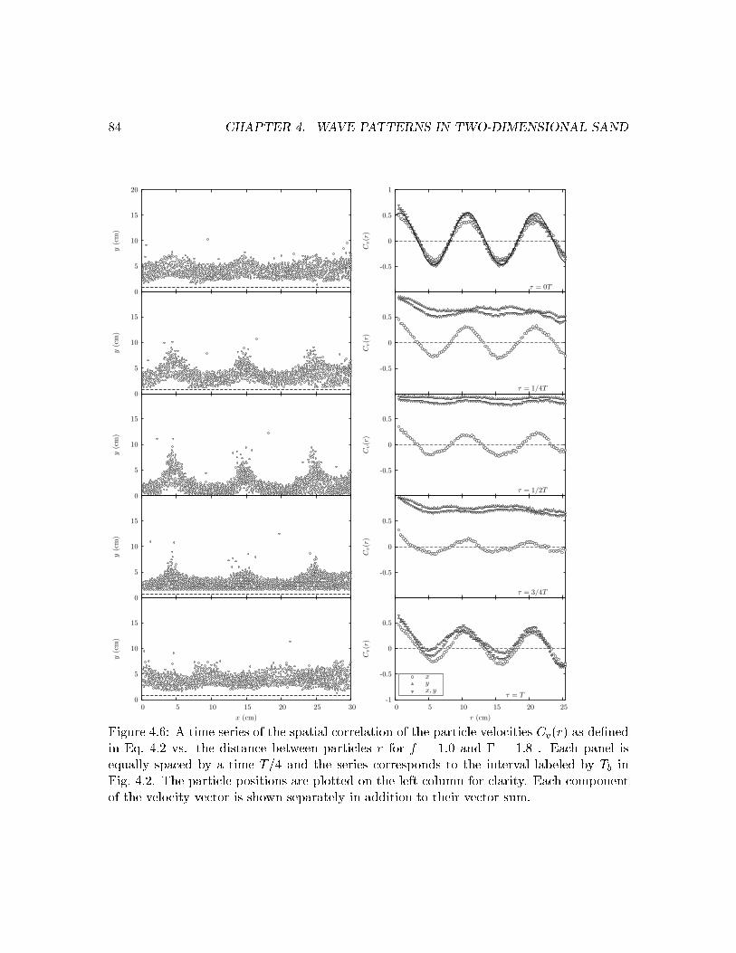
84 CHAPTER 4. WAVE PATTERNS IN TWO-DIMENSIONAL SANDy
(cm
)
20
15
10
5
0
y(c
m)
15
10
5
0
y(c
m)
15
10
5
0
y(c
m)
15
10
5
0
x (cm)
y(c
m)
302520151050
15
10
5
0
τ = 0T
Cv(r
)
1
0.5
0
-0.5
τ = 1/4T
Cv(r
)
0.5
0
-0.5
τ = 1/2T
Cv(r
)
0.5
0
-0.5
τ = 3/4T
Cv(r
)
0.5
0
-0.5
x, yyx
τ = T
r (cm)
Cv(r
)
2520151050
0.5
0
-0.5
-1Figure 4.6: A time series of the spatial orrelation of the parti le velo ities Cv(r) as de�nedin Eq. 4.2 vs. the distan e between parti les r for f = 1:0 and � = 1:8 . Ea h panel isequally spa ed by a time T=4 and the series orresponds to the interval labeled by Tb inFig. 4.2. The parti le positions are plotted on the left olumn for larity. Ea h omponentof the velo ity ve tor is shown separately in addition to their ve tor sum.

4.3. PATTERNS AT (F=2) 85y
(cm
)
20
15
10
5
0
y(c
m)
15
10
5
0
y(c
m)
15
10
5
0
y(c
m)
15
10
5
0
x (cm)
y(c
m)
302520151050
15
10
5
0
y(c
m)
20
15
10
5
0
y(c
m)
15
10
5
0
y(c
m)
15
10
5
0
y(c
m)
15
10
5
0
x (cm)
y(c
m)
302520151050
15
10
5
0Figure 4.7: A time series of the velo ity �elds for the pattern formed at f = 1:0 and � = 1:8, orresponding to the same interval of Fig. 4.6. Ea h velo ity ve tor is the mean velo ity ina 0:9 m2 area.
86 CHAPTER 4. WAVE PATTERNS IN TWO-DIMENSIONAL SANDTherefore, we propose the following form to des ribe the orrelation fun tionCv(r) = A sin�2�r�o + ��; (4.3)where A = �1=2, and �o and � are free parameters. We observe from a least squares �tto Eq. 4.3, that �o = 10:1 m orresponds to an a urate measure of the wavelength of thepattern. The fa t that the ve tor sum re e ts the identi al form of both omponents inpanel one of Fig. 4.6 implies that ea h omponent is approximately the same magnitude.The physi al me hanism that leads to the sinusoidal form of Cv(r) is learly shown by thevelo ity �eld shown in the �rst panel of Fig. 4.7. By visual inspe tion of the velo ity ve tors,one an immediate dis ern that at intervals of �=2 the velo ity ve tors rotate by � and atdistan es of � the ve tors have rotated by 2�. Therefore, from the de�nition of the Cv(r) asthe osine of the angle between velo ities, the phase shifted sinusoidal form is obvious. WhenCv(r) follows the form of Eq. 4.3, the pattern is at it's maximal rearrangement, and all ofphase spa e dire tly re e ts the spatial periodi ity that is normally only asso iated with thepositions of the parti les during pattern formation. The next three panels of Figs. 4.6, 4.7demonstrate that although the mean ow in the y-dire tion dominates, (leading to Cv(r) � 1for both the ve tor sum and the y omponent) Cv(r) for the x omponents still re e t thesinusoidal form given by Eq. 4.3 thus preserving the underlying wavelength of the pattern.We �nd that even the velo ities undergo pattern formation, and in a sense they do so in amore quantitative manner than the parti le positions. That is, there is little ambiguity inthe wavelength that Cv(r) pi ks out.4.4 A Period Doubling Bifur ationOne of the more interesting phenomenon that di�erentiates pattern formation in granular uids from that of Newtonian uids, is the ability of the granular layer to undergo perioddoubling bifur ations. The primary bifur ation arises due to lift-o� of the layer from thedriving plate [10, 151℄. In a onventional Faraday experiment, lift-o� is not possible due tothe no-slip boundary onditions. 1 Period doubling o urs when the a eleration rea hes a riti al value and the the ight time of the bulk of the parti les, with respe t to the drivingwall, be omes double valued. In three dimensional experiments [10, 65, 151℄ on thin layers,(Nl = 5� 10) the initial period doubling bifur ation gives rise to a new set of patterns su has hexagons, and within a narrow regime of phase spa e, at layers os illating at f=2. The at layers an form multiple regions of equal mass (or number of parti les) that os illateout of phase by �. The phase defe ts or \zippers" [65℄, are onsidered topologi al defe ts1Fluids may avitate, therefore opening a gap where they ome into onta t with a ontainer wall, howeverthis would not be the same as lift-o� in the granular analogy.

4.4. A PERIOD DOUBLING BIFURCATION 87center of massright minimum
left minimumdriving wall
t (s)
y(c
m)
543210
6
5
4
3
2
1
0Figure 4.8: Position of the driving wall (solid line), the minimum positions of the leftand right sides (long and short dashed lines, respe tively) and enter of mass of the bulk(dot-dashed line) vs. t in se onds formed at f = 1:0, � = 1:8 .
2Tb
(f/2)
2Ta
t/T
y(c
m)
43210
4
3
2
1
0
Figure 4.9: The position of the driving wall and the lowest point of left and right side ofthe layer vs. t=T . The intervals marked 2Ta and 2Tb, of width 2T orrespond to the datain Figs. 4.10 and Figs.4.11{4.12, respe tively (see text).
88 CHAPTER 4. WAVE PATTERNS IN TWO-DIMENSIONAL SANDanalogous to domain walls in ferromagneti materials and give rise to additional se ondaryinstabilities known as super-os illons [32, 65℄.By in reasing the amplitude and frequen y of the driving signal to f = 1:4 and� = 2:8, the material undergoes a period doubling bifur ation to a state where the layeris split into two at regions, separated by an interfa e (or zipper), that are independentlyos illating at f=2 with two distin t phases degenerate by �. In Fig. 4.8, the position ofthe plate (solid line), mean position of the left and right sides (long and short dashes,respe tively), and the enter of mass (dot-dashed line) are plotted as a fun tion of time.We observe that indeed there are two oexisting patterns whose motion is out of phase.The bulk motion of the parti les is in resonan e with the driving wall. The driving wall ise�e tively at hing the layer as it returns from a lofted position and by doing so suppressesthe instabilities that arises due to large impulses at the moment of ollision and thereforethe layer remains at.The portion of the y le marked by 2Ta in Fig. 4.9 denotes the interval of the y le thatthe panels in Fig 4.10 represent. Ea h panel is separated by a time interval orrespondingto T=2. The panels indi ate that the granular temperature remains high within the bulkof the at layers therefore demonstrating that even at the apogees of the motion (see bypanels 1,3,5 in Fig. 4.10) the parti le velo ities remain high although the layer remains quitedensely pa ked. Panels two and four represent the instants that the layers are streamingdo to the in uen e of the driving wall.4.4.1 Surfa e instabilities and orrelationsAs dis ussed above, Melo et al. [151℄, and Blair et al. [32℄, have experimentally investigatedhigh a eleration patterns in three dimensional experiments of thin layers of granular mate-rials, and have modeled the dynami s as analogous to the motion of a ompletely inelasti boun ing ball [153℄. In addition to at states that arise at the period doubling bifur ation, ellular patterns su h as hexagons are also observed to oexist out of phase with respe t tothe boundary separating out of phase layers.By slightly lowering � we observe that surfa e instabilities also arise in the at layers,analogous to shown in the phase diagrams of the three dimensional examples [32℄. In the left olumn of Figs. 4.11 and 4.12 a series of parti le positions orresponding to equally spa edT=2 instants denoted by the interval marked 2Tb in Fig. 4.9. The emergen e of surfa epatterns from the at layers is learly demonstrated again by the orrelation fun tion Cv(r)(see the right olumn of Fig. 4.11). In the �rst panel of Fig. 4.11, Cv(r) re e ts the out ofphase hara ter that is manifest in the velo ities of the parti les. For values of r < 15 m,(i.e. r < 1=2{the ell width) the orrelation re e ts the long range de ay to anti- orrelation.At r � 15 m, Cv(r) = �1, indi ating that for all separations greater than half the ellwidth parti les moving in the y-dire tion are anti-parallel. The ontribution from the x-

4.4. A PERIOD DOUBLING BIFURCATION 89y
(cm
)20
15
10
5
0
y(c
m)
15
10
5
0
y(c
m)
15
10
5
0
y(c
m)
15
10
5
0
x (cm)
y(c
m)
302520151050
15
10
5
0Figure 4.10: Time series of the at layer parti le positions and the temperature maps. Ea hpanel is separated by a time of T=2 and orrespond to the interval marked by 2Ta in Fig. 4.9(time in reases from top to bottom). Ea h side of the pattern that has formed is os illatingout of phase by � and the layer itself has undergone a period doubling bifur ation, wherethe ight time strikes the plate at two unique times. The right olumn is the time seriesfor the orresponding temperature averaged over the period of the pattern.
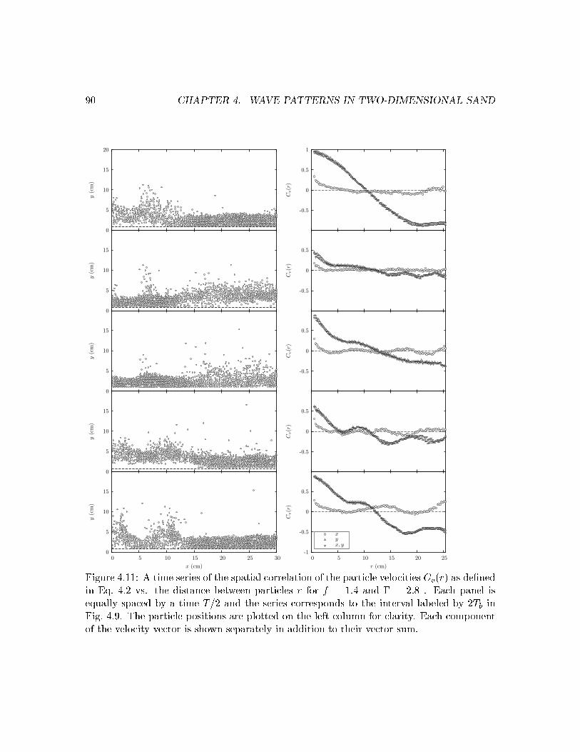
90 CHAPTER 4. WAVE PATTERNS IN TWO-DIMENSIONAL SANDy
(cm
)
20
15
10
5
0
y(c
m)
15
10
5
0
y(c
m)
15
10
5
0
y(c
m)
15
10
5
0
x (cm)
y(c
m)
302520151050
15
10
5
0
Cv(r
)
1
0.5
0
-0.5
Cv(r
)
0.5
0
-0.5C
v(r
)
0.5
0
-0.5
Cv(r
)
0.5
0
-0.5
x, yyx
r (cm)
Cv(r
)
2520151050
0.5
0
-0.5
-1Figure 4.11: A time series of the spatial orrelation of the parti le velo ities Cv(r) as de�nedin Eq. 4.2 vs. the distan e between parti les r for f = 1:4 and � = 2:8 . Ea h panel isequally spa ed by a time T=2 and the series orresponds to the interval labeled by 2Tb inFig. 4.9. The parti le positions are plotted on the left olumn for larity. Ea h omponentof the velo ity ve tor is shown separately in addition to their ve tor sum.

4.4. A PERIOD DOUBLING BIFURCATION 91y
(cm
)
20
15
10
5
0
y(c
m)
15
10
5
0
y(c
m)
15
10
5
0
y(c
m)
15
10
5
0
x (cm)
y(c
m)
302520151050
15
10
5
0
y(c
m)
20
15
10
5
0
y(c
m)
15
10
5
0
y(c
m)
15
10
5
0
y(c
m)
15
10
5
0
x (cm)
y(c
m)
302520151050
15
10
5
0Figure 4.12: A time series of the velo ity �elds for the pattern formed at f = 1:4 and� = 2:8, orresponding to the same interval of Fig. 4.11. Ea h velo ity ve tor is the meanvelo ity in a 0:9 m2 area.

92 CHAPTER 4. WAVE PATTERNS IN TWO-DIMENSIONAL SANDcenter of masslower surfacedriving wall
t (s)
y(c
m)
21.510.50
6
5
4
3
2
1
0Figure 4.13: The position of the driving wall (solid line), minimum position of the layer(dashed line), and the enter of mass of the bulk vs. t in se onds while the parti les areprodu ing f=4 patterns formed at f = 4:0, � = 5:8. The bottom of the layer strikes thedriving wall at the point of maximum upward a eleration. omponents at this instant is very in onsequential to the overall orrelation, as re e tedby the ve tor sum. The out of phase nature of the velo ities is also well re e ted in thevelo ity �eld (see panel one of Fig. 4.12). As time progresses, the layer os illating on theleft side begins to undergo an instability that leads to a distin t pattern with a wavelength� = 7:5 m, or a quarter of the width of the apparatus. The orrelation fun tion also re e tsthe onset of patterns as demonstrated by both velo ity omponents showing a sinusoidaltype os illation.4.5 Patterns at (f=4)As � is in reased further we observe a transition that is also demonstrated by three di-mensional systems. If the a eleration of the plate is high enough the olle tion of grainsis lofted so high that the driving wall an undergo an entire os illation before the layersreturn. By in reasing the frequen y to f = 4:0 Hz and hanging the driving amplitude to� = 5:8 with Nl = 10, we observe a se ond set of standing wave patterns, (two-dimensionalstripes) that are very similar to those presented in Se . 4.3. In Fig. 4.13 the piston position(solid line), the minimum position of the bulk of grains (dashed line), and the enter of mass

4.6. DISCUSSION 93of the bulk (dot-dashed line) are plotted as a fun tion of time. The pattern now requiresfour os illations of the driving wall to return to the original on�guration, therefore makingthe pattern f=4.4.6 Dis ussionIn this Chapter, a set of experiments were ondu ted that produ ed pattern forming statesin granular material on�ned to roll in two dimensions on a subs-trait. The patterns ob-served are similar to those found in previous two- and three-dimensional experiments. Wedemonstrate that under the orre t driving onditions f=2 and f=4 standing waves are pro-du ed, as well as a period doubling bifur ation that leads to zippers and se ondary wavepatterns. By using high speed digital imaging and parti le tra king, long time informationabout the traje tories of the parti les was measured. Unlike gravity waves in onventional uids, where the uid elements follow open parabolas indu ed by a sloshing mode, granular uids follow inverted parabolas whose widths are small ompared to the wavelength. Thetraje tories also demonstrate that the mean free path of a parti le within the layer is mu hlonger than that of a gas at a similar density. The granular temperature is found to varyrapidly during ea h y le of the drive, rea hing nearly zero as the layer re-arranges whileat it's apogee. By measuring the spatial orrelation of the velo ities for snapshots in time,we demonstrate an a urate method of determining the wavelength of the pattern formed,and that the patterns exist in ea h omponent of the phase spa e.


95Chapter 5Magnetized Granular Materials5.1 Introdu tionGranular materials in their simplest form intera t only during onta t. In addition tothe hard- ore repulsion, the oeÆ ients of normal and tangential inelasti ity, and slidingfri tion determine the dissipative intera tion between parti les. Complex properties rangingfrom solid to liquid-like transitions may o ur solely due to these intera tions [189℄. Thereexist numerous ontexts where granular materials have relevan e, and a large number ofthose involve intera tions between the parti les that go beyond those just outlined. Forexample, the presen e of humidity introdu es apillary bridges between parti les resultingin ohesive for es whi h a�e t pa king, ow, and segregation properties [100, 193, 208℄.Capillary intera tion is relatively short range and is important when parti les are nearlyin or leaving onta t. An example where parti les intera t at long range o urs when theybe ome magnetized where intera tion potential is anisotropi . Magneti intera tions areimportant in appli ations ranging from mi ro-sized toners to the pro essing of entimeter-sized mineral ores. Therefore, it is surprising that very few fundamental studies have been ondu ted on the impa t of magneti �elds on the properties of granular materials. Re entex eptions being the work of Forsyth, et al. [83℄, who examined the e�e t of an appliedmagneti �eld on the pa king and ohesivity of a pile omposed of steel beads, and thework of Tazekas, et al. [207℄, who simulated the patterns formed as magnetized parti lesare poured into a silo.Although a omplete theory des ribing the observed phenomena in granular materialsthat in ludes even the basi intera tions is not yet available, interesting progress is beingmade in the regime of low dissipation and rapid motion. In this limit, the kineti theoryof gases has been modi�ed to in lude dissipation [95, 114℄ and experiments have be omeavailable to guide the development of the models [35, 141, 168, 192℄. Therefore, we hosesu h a \granular gas" as the starting point to understand the e�e ts of added magneti

96 CHAPTER 5. MAGNETIZED GRANULAR MATERIALSintera tions. In the limit where the dissipative intera tion an be redu ed to zero, the systemunder onsideration an be mapped to the dipolar hard sphere model [68,190℄. Considerabletheoreti al work has been a omplished using the tools of equilibrium statisti al me hani swhi h an serve as a referen e point in our understanding of the impa t of magnetizationon weakly dissipative granular system.In this hapter, we dis uss an experimental study of model magnetized granular sys-tem �rst introdu ed by us in Ref. [33℄. The system onsists of a vibrated ontainer witha sub-monolayer of uniformly magnetized steel spheres. The experiments are of parti ularinterest due to the dire t visualization of parti les. A granular gas is observed at highvibration amplitudes, and magnetization of the parti les appears to be insigni� ant. In ontrast, when the vibration is lowered below a riti al value, simple hain and ring stru -tures are observed to initially self-assemble be ause of the anisotropi intera tions betweenthe parti les. These stru tures grow rapidly to form either ompa t lusters or networks of hains depending on the depth of the quen h.We ompare and ontrast our results with the dipolar hard sphere model whi h ne-gle ts dissipative intera tions. The model predi ts a network of hains to form below a riti al temperature based on the propensity of the parti les to align along the magneti poles, energy osts asso iated with free ends and entropi onsiderations. Network stru -tures are observed in our experiments, but are metastable. The stable lusters are generallymore ompa t than anti ipated in the models. We measure the velo ity of the parti les andthus the granular temperature to understand the sour e of the dis repan y. Equipartition isnot observed as the temperature of the parti les in the luster is signi� antly lower than thetemperature of the isolated parti les. We dis uss the e�e t of dissipation on the observedphases, and ompare our results with those for the equilibrium dipolar hard sphere model.5.2 Ba kground: dipolar hard spheresWe begin by dis ussing the dipolar hard sphere model (DHSM) whi h serves as an ex-tremum model for parti les with anisotropi intera tions and its impli ations. Developedto understand the kineti behavior asso iated with ferro- uids [68, 190℄, DHSM has seena resurgen e of simulations and theoreti al treatments that have mainly fo used on thequestion of the existen e of a riti al liquid-gas transition [134℄.The idealized intera tion between two dipolar hard spheres separated by distan e ris de�ned as, Udhs = Uhs + 1r3 (~�i � ~�j)� 3r5 (~�i � ~rij)( ~�j � ~rij); (5.1)where Uhs orresponds to the hard ore repulsion intera tion, ~� is the dipole moment, and~r is the inter-parti le ve tor onne ting the enters of dipoles i; j. Clearly from an energypoint of view, neighboring parti les like to align head to tail whi h lowers their energy
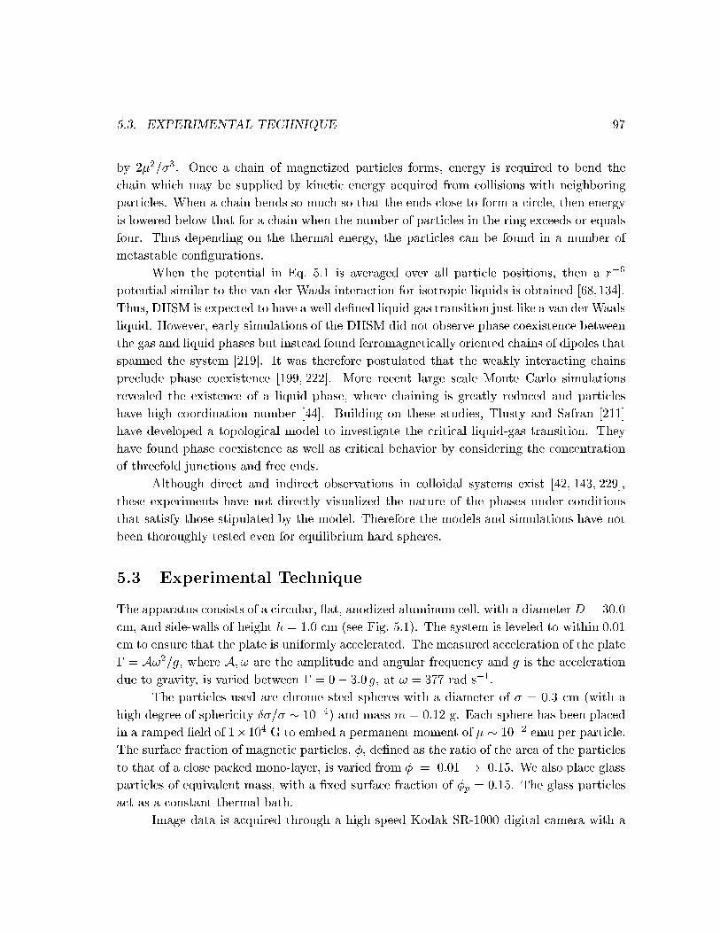
5.3. EXPERIMENTAL TECHNIQUE 97by 2�2=�3. On e a hain of magnetized parti les forms, energy is required to bend the hain whi h may be supplied by kineti energy a quired from ollisions with neighboringparti les. When a hain bends so mu h so that the ends lose to form a ir le, then energyis lowered below that for a hain when the number of parti les in the ring ex eeds or equalsfour. Thus depending on the thermal energy, the parti les an be found in a number ofmetastable on�gurations.When the potential in Eq. 5.1 is averaged over all parti le positions, then a r�6potential similar to the van der Waals intera tion for isotropi liquids is obtained [68,134℄.Thus, DHSM is expe ted to have a well de�ned liquid-gas transition just like a van der Waalsliquid. However, early simulations of the DHSM did not observe phase oexisten e betweenthe gas and liquid phases but instead found ferromagneti ally oriented hains of dipoles thatspanned the system [219℄. It was therefore postulated that the weakly intera ting hainspre lude phase oexisten e [199, 222℄. More re ent large s ale Monte Carlo simulationsrevealed the existen e of a liquid phase, where haining is greatly redu ed and parti leshave high oordination number [44℄. Building on these studies, Tlusty and Safran [211℄have developed a topologi al model to investigate the riti al liquid-gas transition. Theyhave found phase oexisten e as well as riti al behavior by onsidering the on entrationof threefold jun tions and free ends.Although dire t and indire t observations in olloidal systems exist [42, 143, 229℄,these experiments have not dire tly visualized the nature of the phases under onditionsthat satisfy those stipulated by the model. Therefore the models and simulations have notbeen thoroughly tested even for equilibrium hard spheres.5.3 Experimental Te hniqueThe apparatus onsists of a ir ular, at, anodized aluminum ell, with a diameter D = 30:0 m, and side-walls of height h = 1:0 m (see Fig. 5.1). The system is leveled to within 0.01 m to ensure that the plate is uniformly a elerated. The measured a eleration of the plate� = A!2=g, where A; ! are the amplitude and angular frequen y and g is the a elerationdue to gravity, is varied between � = 0� 3:0 g, at ! = 377 rad s�1.The parti les used are hrome steel spheres with a diameter of � = 0:3 m (with ahigh degree of spheri ity Æ�=� � 10�4) and mass m = 0:12 g. Ea h sphere has been pla edin a ramped �eld of 1�104 G to embed a permanent moment of � � 10�2 emu per parti le.The surfa e fra tion of magneti parti les, �, de�ned as the ratio of the area of the parti lesto that of a lose pa ked mono-layer, is varied from � = 0:01 ! 0:15. We also pla e glassparti les of equivalent mass, with a �xed surfa e fra tion of �p = 0:15. The glass parti lesa t as a onstant thermal bath.Image data is a quired through a high speed Kodak SR-1000 digital amera with a

98 CHAPTER 5. MAGNETIZED GRANULAR MATERIALS
Shaker
Accelerometer
CCD
30 cm
10cm
Lock in Amplifier
Amplifier
ComputerFigure 5.1: A s hemati diagram of the experimental apparatus. The plate has a diameterof D = 30 m with side-walls of height h = 1:0 m. The plate is leveled to within 0.01 mto ensure that the a eleration is uniform. The shaker is driven with a power ampli�er andthe driving signal originates from an arbitrary wave form generator. A lo k-in ampli�er�lters the signal of a 10 mV/g a elerometer that is mounted to the bottom of the drivingplate. Image data is a quired from overhead through with a high speed digital amera.Ea h devi e is interfa ed via a mi ro omputer workstation.spatial (temporal) resolution of 512 � 480 pixels (250 frames s�1). By utilizing the Hoshen-Kopelmen algorithm [101℄, individual lusters that form are identi�ed. Having identi�edparti les as members of lusters, the number of parti les, the entroid, and the radius ofgyration an be measured as a fun tion of time. The frame rate is suÆ iently rapid thatinstantaneous velo ities of the parti les an be measured.In any dis ussion of phases in hard sphere systems, the two most important param-eters are the volume fra tion (or area fra tion in a quasi-two dimensional system) and thetemperature. Driven granular systems are non-equilibrium, making the thermal energys ale is irrelevant to the properties at the ma ros opi level. Therefore, a kineti quantity alled the \granular temperature" has been postulated as equivalent to the thermodynami temperature in equilibrium systems [166℄. The granular temperature is given by the widthof the velo ity distribution of the grains. In our experimental system, the parameter we andire tly ontrol is the vibration strength �. We use the glass parti les to de�ne a systemtemperature by performing alibration experiments as a fun tion of �. Energy equipartitionis not observed in systems out of equilibrium, therefore are must be taken while interpret-ing the granular temperature. We will hopefully larify these distin tions at appropriatepoints within the dis ussion.

5.3. EXPERIMENTAL TECHNIQUE 99φ = 0.09φ = 0.05φ = 0.01 (a)
Γ = 2.0
v (cms−1)
P(v
)
403020100-10-20-30-40
10−1
10−2
10−3
10−4
10−5
φ = 0.09φ = 0.05φ = 0.01
Γ/g
T[g
(cm
s−1)2
]
2.42.22.01.81.61.41.2
9.0
8.0
7.0
6.0
5.0
4.0
3.0
2.0Figure 5.2: (a) The distribution of parti le velo ities of the P (vx) versus vx, omponent ofthe velo ity in the horizontal dire tion for � = 2:0 , at � = 0:01; 0:05; 0:09. The distributionshave not been res aled, thus demonstrating that over a broad range of surfa e fra tion thedistribution is un hanged. The solid line is a Gaussian �t for � = 0:09. (b) The granulartemperature T , versus �, the dimensionless a eleration. The data is essentially independentof �. The distribution of parti le velo ity omponents in the horizontal dire tion is shownin Fig. 5.2(a) for three values of � at a �xed ! and � = 2:0. The data orresponding to bothglass and steel parti les in the gas-like state. Be ause the mass of the parti les were hosento be similar, their distributions are found to be identi al over a broad range of surfa efra tion. The distributions are non-Gaussian, onsistent with previous observations [141℄,and have a kurtosis of 3.73 (a Gaussian distribution has a kurtosis of 3.0). Due to theself- onsisten y of the distributions, we an de�ne the granular temperature as follows:T = 32mhv2i i; (5.2)where i represents the individual omponents of the velo ity ve tor. Here we have assumedthat the velo ity distributions in the horizontal and verti al dire tions are the same, al-though in reality it may be di�erent by a fa tor given by the oeÆ ient of restitution [35℄.Using this de�nition, we have obtained the granular temperature as a fun tion of � [seeFig. 5.2(b)℄. We observe that the points (to within experimental a ura y) fall onto onemaster urve irrespe tive of �. The resulting alibration allows us to simply utilize a lo al�tting window on the points in Fig. 5.2(b) to obtain the temperature of the bath T by onlyknowing �. We will see in a later se tion that the temperature of the magnetized parti lesis in fa t not the same as the bath temperature but state-dependent.

100 CHAPTER 5. MAGNETIZED GRANULAR MATERIALS(a) (c)(b)Figure 5.3: Initial stru tures that nu leate from the gas phase at and below Ts. (a) A hainof dipoles that rapidly evolves into a more stable and energeti ally favorable on�guration.(b) A ring of 13 dipoles ( ) A lose pa ked luster. The s ale bar denotes 1 m. T = 4:0erg, � = 0:09(a) (b) (c)Figure 5.4: The evolution of a hain at � = 0:05, T = Ts over t = 1080 s. The hain beginsas a extended stru ture, (a) that formed from multiple short hains joining together and intime be ame more ompa t. The white s ale bar denotes 1 m.5.4 The Phase DiagramTo study the transition from a gas to a lustered phase, experiments with the followingproto ol are performed. The ontainer with the a �xed number of parti les is �rst vibratedat high amplitude (� = 3) so that a gas-like state is observed and then the amplitude islowered. Below a riti al amplitude, lusters nu leate and grow. The order of magnitudewhere the transition o urs an be determined by onsidering the temperature of the systemand the dipole energy 2�2=�3. We denote the temperature that lusters are �rst observedto nu leate as the transition temperature Ts. As Ts is approa hed from above, (i.e. bylowering T from the gas temperature), prior to a tual nu leation, the system begins tosupport the existen e of short lived di-mers and tri-mers that a t as the initial seeds for thenu leating lusters. In Fig. 5.3(a{ ) typi al initial stru tures are shown. The formation andgrowth of these initial stru tures depends on the bath temperature to whi h the system islowered to.When the vibration amplitude is lowered to Ts or slightly below, we observe thatlong hains, like those found in Fig. 5.3(a) are unstable, and in time will give way to

5.4. THE PHASE DIAGRAM 101
0.00 0.05 0.10 0.15φ
0.0
2.0
4.0
6.0
8.0
Tg
[ g (
cm s-1
)-2
]Gas
Clustered
0.0
0.5
1.0
1.5
2.0
2.5
Γ
�������������������������������������������������������������������������������������������������������������������������������������������������������������������������������������������������������������������������������������������������������������������������������������������������������������������������������������������������������������������������������������������������������������������������������������������������������������������������������������������������������������������������������������������������
�������������������������������������������������������������������������������������������������������������������������������������������������������������������������������������������������������������������������������������������������������������������������������������������������������������������������������������������������������������������������������������������������������������������������������������������������������������������������������������������������������������������������������������������������
������������������������������������������������������������������������������������������������������������������������������������������������������������������������������������������������������������������������������������������������������������������������������������������������
������������������������������������������������������������������������������������������������������������������������������������������������������������������������������������������������������������������������������������������������������������������������������������������������
Network
Hysteresis
Figure 5.5: The phase diagram of temperature T versus the surfa e fra tion of the parti les�. The driving a eleration �, is also shown for larity. A gas phase onsisting of singleparti les and short lived di-mers and tri-mers are observed above a transition temperatureTs that depends on �, shown by the solid points. To evaporate a luster in the gas phase onemust go past Ts denoted by the hysteresis region. At and below Ts, di-mers and tri-mersa t as seeds to the formation of ompa t lusters that oexist with single parti les. If T israpidly quen hed from the gas region to very low T highly rami�ed networks of parti lesform [Fig. 5.6( )℄.more ompa t stru tures. Chains of parti les will either form ring on�gurations, or more ompa t on�gurations [see Fig. 5.3(b, )℄. There are at least two possible s enarios for the hange from the hain on�guration: (1) Chains are highly mobile. Mobility, due to therotational and translational degrees of freedom, allow hains to align head-to-tail and growthrough a oarsening pro ess. (2) Due to the exibility of the hains, and the long-rangeattra tive intera tions of their free ends, they will eventually atta h themselves either toanother hain or will form a loop or a losed Y [see Fig. 5.3(b)℄.The pro ess des ribed as s enario (1) above is displayed in Fig. 5.4(a{ ) for a par-ti ular hain at T = Ts. Initially, the hain [Fig. 5.4(a)℄ onsists of the beginnings of aY stru ture at the top and a ring of four parti les in the enter. Figure 5.4(b) shows anintermediate on�guration, and Fig. 5.4( ) shows the luster after 1080 s that oexists withindividual parti les.To hara terize the gas and lustered phases des ribed above, and to des ribe the

102 CHAPTER 5. MAGNETIZED GRANULAR MATERIALS
(a)
(b)
(c)Figure 5.6: Images of the observed phases. (a) The gas phase for T = 7:5 erg, � = 0:09.(b) The luster phase T = Ts, � = 0:09. ( ) The network phase after a rapid quen h fromT = 7:5! 3:3 erg, � = 0:15nature of the transition, we plot the phase diagram (see Fig. 5.5). The onne ted pointsre e t the measured transition temperature Ts, that separates the gas phase [Fig. 5.6(a)℄from the lustered phase [Fig. 5.6(b)℄, and demonstrates a monotoni in rease with �. If lusters are nu leated and T is then in reased above Ts, lusters evaporation is hystereti .The apparent hysteresis depends on the ramping rate of T , and is not observed to disappearover laboratory time-s ales. Therefore, it appears that the observed phase transition is �rstorder.Within the luster phase, there exists a large network phase (see Fig. 5.5) that isprodu ed by rapidly quen hing the system from dire tly from the gas phase far below Ts.The result of su h a rapid thermal quen h is shown in Fig. 5.6( ).The qualitative features of the network phase an be understood as follows. Whenthe system is quen hed, the kineti energy of the parti les is dramati ally de reased, andthe e�e ts of the long range dipole potential be omes important. Energeti ally, the lo alarrangement is dominated by head-to-tail alignment due to the inherent anisotropy in theembedded potential (see Eq. 5.1). As dis ussed earlier, from the energy standpoint it is farmore favorable to form ring and ompa t states when the number of parti les in a hainrea hes four. However, at low temperatures, the probability that a hain re eives signi� antkineti energy to over ome the bending potential barrier de reases. Thus the metastable hain like stru tures an be observed over long times. Consequently, the further we lower thetemperature in the quen h, the stru ture formed is more rami�ed and survives as su h for alonger time. Over very long times, the on�guration evolves and the eventual on�gurationis a more ompa t luster with very few free ends.The reason why the network phase may be interpreted as a metastable liquid an be

5.4. THE PHASE DIAGRAM 103
(b)
r/σ
g(r
)
543210
12
10
8
6
4
2
0
(a)
g(r
)
16
14
12
10
8
6
4
2
0
Figure 5.7: The radial distribution fun tion g(r) vs r=� for the (a) lustered and (b) networkphases. In the luster phase, [see Fig. 5.6(a)℄ a splitting of the se ond and third peakswhi h indi ates the existen e of short range stru ture. The network phase demonstrates hara teristi s asso iated with liquids. The parameters for the plots are (a) � = 0:09,T = 5:8 erg and (b) � = 0:15, T = 2:9 erg.

104 CHAPTER 5. MAGNETIZED GRANULAR MATERIALS
v (cms−1)
P(v
)
403020100-10-20-30-40
10−1
10−2
10−3
10−4
Figure 5.8: The probability distribution fun tions P (v) of the velo ity omponents in thegas and lustered phases on a log linear s ale. (O) dipolar parti les in a purely gas phaseat T = Ts and � = 0:09 just prior to a luster nu leating, (4) glass parti les at T = Ts and� = 0:15, (�) magneti parti les that oexist in the gas phase with a luster at � = 0:09T = Ts, (Æ) parti les within the luster at T = Ts and � = 0:09. The solid lines are Gaussian�ts. Even though the phases oexist, velo ity distribution of parti les in the gas phase aresigni� antly greater than that for the lustered phases.shown as follows. We plot the radial distribution fun tion of parti le positions,g(r) = 1N N Xn=0 1N2 NXi NXj 6=i Æ(r � rij)�rÆr ; (5.3)where rij is the inter-parti le spa ing and N is the number of separate on�gurationssampled for the parti les in a luster at T = Ts and for a network (see Fig. 5.7(a),(b)respe tively). Like the g(r) for a liquid, the plot shows peaks at unit intervals.5.5 The Non-Equipartition of EnergyBefore ontinuing the systemati exploration of the phase diagram, we �rst dis uss theimpa t of the magneti �elds on the velo ity distributions and onsequently the granulartemperature. By using the parti le tra king and luster identi� ation methods utilized inSe tion 5.3 we measure the temperature of the parti les with the lusters. In Fig. 5.8 thedistribution of parti le velo ities for various spe ies is shown. The spe ies of the parti les are

5.6. CLUSTER GROWTH RATES 105
r/σ
Tc
[g
(cm
s−1)2
]
302520151050
0.12
0.10
0.08
0.06
0.04
0.02
0.00Figure 5.9: The luster temperature T vs. r=� for � = 0:09. The temperature of the lusterde reases as fun tion of time and therefore as a fun tion of luster size.de�ned by the phase that the parti les exist in. The three broad distributions orrespondto the following spe ies: Dipolar parti les in a purely gas phase at T = Ts and � = 0:09 justprior to a luster nu leating, given by (O). The glass parti les at T = Ts and � = 0:15 givenby (4). The magneti parti les that oexist in the gas phase with a luster at � = 0:09T = Ts given by (�). The parti les within the luster at T = Ts and � = 0:09 given by(Æ). The distributions are shown in absolute units, demonstrating that when parti les arein a gas phase, prior to and after a luster has nu leated, their granular temperatures arewell de�ned and equipartition holds. However, on e parti les enter a luster, their motionis highly limited thus the redu tion in their kineti de�ned temperature.We also observe that as lusters in fa t ool as their size in reases. In Fig. 5.9 thetemperature of a luster at T = Ts and � = 0:09 is shown versus its radius. The ratio ofthe luster temperature T to that of the system temperature T , is T=T � 60. Therefore,both the mobility or di�usion of parti les has been redu ed, (not unlike the analog of olloidal gels) and the mean square velo ity no longer re e ts the mean square velo ityof the system. Thus we have demonstrated the apparent breakdown of equipartition in amagnetized granular system.5.6 Cluster Growth RatesWe now dis uss how the lusters grow on e they are nu leated. It is observed that the loserthe temperature is to Ts the fewer lusters nu leate; onversely, more lusters nu leate the
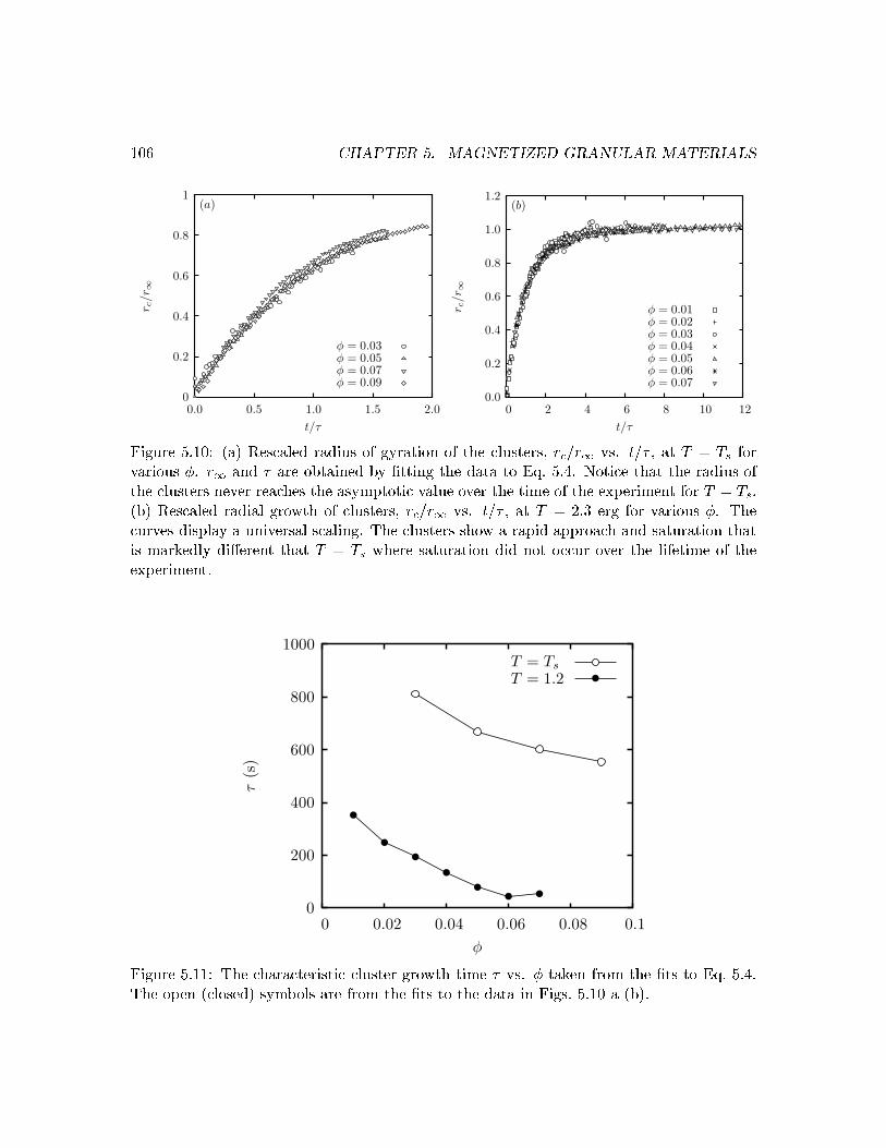
106 CHAPTER 5. MAGNETIZED GRANULAR MATERIALS
φ = 0.09φ = 0.07φ = 0.05φ = 0.03
(a)
t/τ
r c/r ∞
2.01.51.00.50.0
1
0.8
0.6
0.4
0.2
0φ = 0.07φ = 0.06φ = 0.05φ = 0.04φ = 0.03φ = 0.02φ = 0.01
(b)
t/τ
r c/r ∞
121086420
1.2
1.0
0.8
0.6
0.4
0.2
0.0Figure 5.10: (a) Res aled radius of gyration of the lusters, r =r1 vs. t=� , at T = Ts forvarious �. r1 and � are obtained by �tting the data to Eq. 5.4. Noti e that the radius ofthe lusters never rea hes the asymptoti value over the time of the experiment for T = Ts.(b) Res aled radial growth of lusters, r =r1 vs. t=� , at T = 2:3 erg for various �. The urves display a universal s aling. The lusters show a rapid approa h and saturation thatis markedly di�erent that T = Ts where saturation did not o ur over the lifetime of theexperiment.T = 1.2T = Ts
φ
τ(s
)
0.10.080.060.040.020
1000
800
600
400
200
0Figure 5.11: The hara teristi luster growth time � vs. � taken from the �ts to Eq. 5.4.The open ( losed) symbols are from the �ts to the data in Figs. 5.10 a (b).

5.6. CLUSTER GROWTH RATES 107further the temperature is lowered below Ts. Therefore, we �rst dis uss the growth whenthe temperature of the gas phase is lowered so that T = Ts, and then dis uss the lustergrowth at lower onstant temperature. By arefully lowering the temperature to Ts we areable to nu leate a single luster (if a single luster does not form the pro ess is repeated).We observe that the hange of the radius of gyration is well des ribed by a simpleexponential form, r = r1(1� e�t=� ); (5.4)where r1 is the asymptoti radius, and � is the saturation time. By res aling ea h dataset shown in Fig. 5.10(a) by the asymptoti radius and the saturation time we demonstratethat the growth equation is universal. The values of � are plotted versus � in Fig 5.11. Italso appears that the lusters formed at T = Ts never rea h their asymptoti radius in thepresent experimental time window.The saturation of the radius of gyration o urs be ause the total number of magne-tized parti les de reases at a rate n(t) = (N � n (t)1=d), where N is the total number ofparti les and d is the fra tal dimension of the luster. We never observe that all of the freeparti les join the luster. However, the overall surfa e fra tion is lowered by the lustergrowth, therefore leading to a redu tion of the growth. We spe ulate that there may alsobe se ondary e�e ts that further a t to arrest the growth, su h as hanges in the urvatureof the outer edge of the luster, and the shielding of the lusters by the side walls.In the previous paragraph and in Fig. 5.10(a) we demonstrated that the luster radiusnever rea hed r1 for all �. To investigate the response of the system to temperatures belowTs, we have lowered the temperature of the system from the gas phase to the isothermT = 2:3 erg for � = 0:01 � 0:07.We observe that by lowering the temperature to slightly below T at that parti u-lar �, luster nu leation is quite rapid as ompared to the observations made at Ts [seeFig. 5.10(b)℄. Also, the number of lusters formed ranges from n = 1 � 5 depending onthe surfa e fra tion, but does not follow any systemati trend. The radial growth equation(Eq. 5.4) is also �t to the data and demonstrates a rapid growth to a saturation value de-termined by �. In Fig. 5.10(b) the evolution of the radius of gyration is res aled for all � isplotted. The good ollapse of the urves further indi ating a universal form given by Eq. 5.4.The hara teristi time � is plotted as a fun tion of � (see Fig. 5.11) and demonstrates alinear de rease in over a broad range of surfa e fra tions.We do note however that at temperatures far below Ts the saturation to r = r1does indeed o ur unlike the data presented at T = Ts where the saturation was limitedby oexisten e. We interpret this saturation as an e�e t of dissipation. Due to the loweredtemperature, parti les that remain in the gas phase are less likely to impa t the lusterswith large velo ities. Thus, the thermal parti les are less likely to remove parti les from the lusters. This, oupled with the dissipation due to ollisions and the attra tive intera tions

108 CHAPTER 5. MAGNETIZED GRANULAR MATERIALS
φ = 0.09φ = 0.07φ = 0.05φ = 0.03
(a)y = x1.4
y = x2
rc/σ
〈nc〉
101
100
10
1φ = 0.07φ = 0.06φ = 0.05φ = 0.04φ = 0.03φ = 0.02φ = 0.01
(b)
y = x1.5
rc/σ
〈nc〉
101
100
10
1Figure 5.12: (a) The average number of parti les in a luster hn i vs. r =� the radius ofgyration over a range of � at T = Ts. The dashed lines indi ate two unique s alings forthe dimensionality of ea h luster demonstrating a rossover at r =� = 6. (b) The averagenumber of parti les in a luster hn i vs. r =� the radius of gyration over a range of � atT = 2:3 erg. The dashed lines indi ates a single s aling that aptures the overall s aling ofthe lusters.between parti les, leads to a rapid approa h to r1 for all �.5.7 Compa tness of the ClusterIn Fig. 5.12 the average number of parti les ontained in a luster hn i = n =n, where n isthe total number of lusters formed, is plotted versus the dimensionless radius of gyrationr =�. We propose a general de�nition for n , as an average value, be ause the same quantitywill be used when multiple lusters form (when T = Ts, n = 1). By using the s aling relationn = �Rdg ; (5.5)where � is determined by the dimensionality of the mass elements, (for disks � = �2=2p3)awe al ulate the fra tal dimension of the lusters.Figure 5.12(a) learly demonstrates a rossover in the dimensionality of the lusters.Clusters with r < 5:0� follow losely to the spatial dimension. As the number of parti lesper luster in reases with time the trend for the fra tal dimension, d, over all �, is more onsistent with d = 1:4�0:1. Thus we demonstrate that lusters are initially more ompa tand isotropi at early times, and be ome more extended for long times at T = Ts.The hange in dimensionality may be understood by observing the growth of a luster.As parti les join the luster they do so by forming highly mobile hains that are tethered

5.8. MIGRATION OF CLUSTERS 109
x (cm)
y(c
m)
302520151050
30
25
20
15
10
5
0Figure 5.13: The traje tory of the enter of mass of a luster in the ell. The solid linerepresents ea h spa e time point for the luster enter of mass. The dashed line denotes theinner boundary of the ell, while the individual points show the �nal spot of the parti leswithin the luster at the end of the experiment.by one end to the surfa e of the luster. If the free end of the hain is able to onne tba k onto the luster an ex luded area is established. During this pro ess free parti les maybe ome trapped by the hains. The trapped parti les an, in time, produ e rearrangementand re-opening of these regions. The fra tal-like hara ter of the lusters an be seen inFigs. 5.6(b), and 5.13.We also measure the fra tal dimension of the lusters at T = 2:3 erg. In Fig. 5.12(b)the radius of gyration r , s aled by the parti le diameter, of ea h luster is plotted versusthe number of parti les within the luster. We observe that the fra tal dimension has avalue of d � 1:5, that does not depend on the surfa e fra tion.The nature of the lusters is quite di�erent than those measured at Ts. First, the lusters have a onstant and somewhat larger fra tal dimension. Se ond, due to the mu hlower system temperature, the parti les are less likely to rearrange on e they have joinedinto the lustered phase and as a onsequen e the motion of the lusters is very small ompared to the example shown in Fig. 5.13.

110 CHAPTER 5. MAGNETIZED GRANULAR MATERIALS5.8 Migration of ClustersNext we omment on the interesting dynami s of the luster as a whole. Soon after lustersform, they an nearly always observed to migrate towards the ontainer boundary. Thetraje tory of a luster over time migration is shown in Fig. 5.13; the positions of the parti leswithin the luster at time t = 1100 s is also plotted. Soon after the luster forms, it di�usesuntil it rea hes the boundary. The absen e of \thermal" parti les near the side wall results inan unbalan ed pressure whi h pins the luster to the side wall. On e in onta t, the lusterdemonstrates the existen e of a depletion for e as seen in olloids [118℄. The depletant inthis ase is the \thermal" parti les (magneti and glass) impinging on the side of the luster.5.9 SummaryWe have introdu ed a new experimental system to study the impa t of magneti intera tionson granular systems. The parti les intera t via their magneti �elds and inelasti ollisions.Using a quasi-two dimensional geometry, we are able to visualize the state of the systemas a fun tion of area fra tion and external driving amplitude. Be ause the intera tions areanisotropi , both simple and omplex stru tures an be made to self-assemble by hangingthe system parameters.We have found that the nature and growth of the lusters depends is history depen-dent. Therefore, the formation of the lusters was explored using two proto ols. When thevibration amplitude is lowered slightly below the riti al amplitude, simple stru tures su has rings or hains formed whi h ontinue to grow adsorbing parti les from the gas phase.The radial growth of the radius of gyration of the luster follows a universal de aying expo-nential form. However the asymptoti radius is never rea hed over laboratory time s ales.The fra tal dimension of the lusters undergoes a rossover from a dimension that mat hesthe spatial dimension to a lower value. The rossover o urs as parti les join the lusterthrough a haining and looping pro ess.If the temperature is lowered below Ts the lusters that nu leate have a very di�erent onformation. The radial growth still universally s ales to a de aying exponential form,but the asymptoti radius is always rea hed. Below Ts, the luster dimensionality does notdemonstrate a rossover but remains �xed at a value somewhat greater than that of lustersat Ts implying that the ompa tness of lusters is always less at lower temperatures.We also observe that within the luster region in the phase diagram there exists anetwork phase that exhibits a metastable liquid hara ter. The network is omprised of par-ti le that are onne ted as hains. These hains demonstrate the inherent anisotropy in theintera tions between parti les. The metastability an be understood from the energy land-s ape that the network must traverse to not only over ome the energy penalty of bendingthe hains but also the dissipation and fri tion that is the hallmark of this non-equilibrium

5.9. SUMMARY 111system.When lusters oexist with single or gas like parti les, we �nd that the granulartemperature of the parti les in the lusters is signi� antly lower than those is the gas phase.Furthermore, the temperature of the parti les in the lusters de reases as its size in reases.Thus equipartition is not observed. The reason for the lower temperature in the lusteredphase appears to be fri tion and inelasti ollision whi h qui kly suppress rapid relativemotion between parti les.Thus we have shown that a granular system with magneti intera tions shows a ri hvariety of phases and phenomena. Using the dipolar hard sphere model, one an understandsome of the observed stru tures. However, a deeper understanding of the dissipative inter-a tions has to rea h to understand why the observed stru tures are more ompa t thanthose predi ted by simulations ondu ted from equilibrium systems. Our study may behelpful in developing mi ro-me hani al devi es where the understanding of pro esses thatlead to self-assembly of omplex stru tures from omponents is of vital importan e.


113Chapter 6The Dynami s of Granular RodsIn all of the previous Chapters experiments were ondu ted with geometri ally isotropi parti les, i.e. spheres. In Chapter 5 however, we extended the our general treatment ofgranular gases by introdu ed a spe i� anisotropy to the parti le intera tion, namely anembedded dipolar potential. In this Chapter, we will again extend the general experimental ondition by introdu ing a new experiment with parti les that possess an inherent shapeanisotropy.Introdu tionRod shaped parti les abound in nature at all length-s ales { from viruses, to trees, to thepen that may be in your hand as you read this do ument (see Fig. 6.1). The ubiquity ofgranular materials is of ourse a well established fa t. Therefore experiments ondu tedto understand the physi s that governs their dynami s are warranted. However, granularmaterials that are found in nature are often not well represented by the simple spheresthat are studied in experiments and simulations. Often, the natural form for granularmatter is a more prolate or rod like in onformation. At mi ro/meso-s opi s ales, whereparti les are thermalized by O(kBT ) energies, su h as rod shaped olloids, the pro ess ofentropi ally driven ordering, mediated by shape, is a well known phenomenon [6, 169℄. Asparti le size in reases to the granular s ale (usually when the parti les size is > 10�m),dissipation through inelasti ity and fri tion dominate the energy lands ape, leading to newand surprising phenomenon. Moun�eld and Edwards [159℄, applied on epts of on�gura-tional statisti al me hani s to study the nature of the isotropi to nemati phase transitionin a granular system of elongated parti les. In re ent experiments utilizing a tall narrow ylinder, Villarruel et al. [225℄ studied the e�e ts of anisotropy on granular pa king. Theyobserved the appearan e of sme ti states with the dire tion given by the ontainer walls.In this Chapter, a set of simple and insightful one-dimensional experiments on gran-

114 CHAPTER 6. THE DYNAMICS OF GRANULAR RODS
(a) (b)
( )Figure 6.1: (a) Image of a the toba o-mosai virus, ea h virus is � 10�m in length. (b)Orzo style pasta with a typi al length of � 1 m. ( ) An image of a \log jam" where ea hparti le is � 10 m.

6.1. EXPERIMENTAL APPARATUS AND PROCEDURE 115Vcc
Camera
Relay
Drop CircuitTriggering and
Camera
Computer
CCD
α
Figure 6.2: S hemati diagram of the apparatus to measure the oeÆ ient of restitution fora single rod. The rod is dropped onto a surfa e of variable in lination angle �. The ameraand the dropping relay are triggered by the ir uit shown in the inset box. Images of therod are transfered to the omputer and analyzed.ular rods is presented and dis ussed. The olle tive phenomenon of driven granular matterhas been of interest sin e the time of Faraday [80℄. Surfa e instabilities leading to pat-tern formation, (dis ussed in Chapter 4) is one su h manifestation of olle tive motion. Todire tly measure the motion of the onstituent parti les undergoing pattern formation wehave utilized an experiment of redu ed dimensionality. Redu ing the system to two dimen-sions allowed for dire t visualization into the single parti le dynami s leading to insightsinto more omplex phenomenon. In this Chapter, a similar approa h is taken with respe tto the phenomenology of vortex motion found in driven granular rods [37℄.6.1 Experimental Apparatus and Pro edureThe oeÆ ient of restitution for a single rodEnergy loss during a ollision is distin tly asso iated with the dynami s of granular materi-als. In Chapter 2 we dis ussed the e�e tive normal oeÆ ient of restitution for a olle tionof spheres that are onstrained to roll on a substrate; the e�e tive restitution oeÆ ientwas measured dire tly with high speed imaging. Here we present an experiment designedto measure the oeÆ ient of restitution for a single rod that ollides with a ridged plate.The experiments are performed in the following way. Using a simple swit h ir uitthat is onne ted to a relay and a high speed amera (see Fig. 6.2), we simultaneouslyrelease a rod and trigger the amera that aptures images at 500 frames s�1. The rod is

116 CHAPTER 6. THE DYNAMICS OF GRANULAR RODS
(a) (b) ( )Figure 6.3: Time sequen e of a rod dropping onto a stainless steel plate at � = 0os. Therod is released (a) t = 0, ollides with the plate (b) t = 146ms, and at the apex of the return( ) t = 296ms.
(a) (b) ( )Figure 6.4: Time sequen e of a rod dropping onto a stainless steel plate at � = 10os. Therod is released (a) t = 0, ollides with the plate (b) t = 138ms, and at the apex of the return( ) t = 266ms. Note that the rod has undergone half a rotation.

6.1. EXPERIMENTAL APPARATUS AND PROCEDURE 117released from the height, ho = 11:0 m, and ollides with a stainless steel or Delrin plate.The plates are held at �xed angles of � = 0o, and � = 10o w:r:t: the horizontal. The anglesare hosen to mimi the dynami s of a rod des ribed in the experiments below. The tip ofthe falling rod is rounded to ensure that spurious rotations are not indu ed due to glan ing ollisions with the plate. However, the rod may slip at the moment of onta t leading to aloss of energy due to fri tion, or if the surfa e is very smooth, the parti les may not boun eat all. Care is also taken to ensure that the rod falls as straight as possible so that initialangular momentum does not have to be onsidered in the following analysis.After the rod is released, the geometri enter is tra ked as a fun tion of time. Addi-tionally, rotations of the rod about it's enter are measured to ensure that energy loss dueto transferen e to angular momentum are onsidered (drag due to air e�e ts is negle ted).In Figs. 6.3 and 6.4 a series of images is presented to demonstrate the release, ollision, andreturn of the parti le. The maximum height, hf , of the rod after olliding with the plate isgiven by hf = fho + I!22Mg ; (6.1)where I =ML2=12 is the moment of inertia of a rod and f is the oeÆ ient of restitution.By keeping the rod as straight as possible, prior to release, the motion is restri ted to the(x; z) plane and the enter of mass has a traje tory along the z-axis. Using Eq. 6.1 we ansolve for f f = hfho � (L!)224g ho : (6.2)The images in Fig. 6.4(a{ ) demonstrate and example of the experiments with the stainlesssteel plate in lined at � = 10o. We typi ally �nd that when the plate is in lined therod undergoes half a rotation, indu ed by fri tion. The approximate value that a halfrotation detra ts from the total energy is more than an order of magnitude smaller thanthe inelasti ity alone, and therefore has a minor in uen e on the total energy loss. Theaverage values for f and the standard deviations for ten experiments, � f are displayedin Table 6.1. The values of the oeÆ ient of restitution demonstrate a dependen e notonly on the material that the parti le intera ts with, but also the angle of in lination. Thephysi al interpretation of the angular dependen e for f is that slipping at the moment of onta t determines the amount of e�e tive energy loss. The stainless steel surfa e is mu hless fri tional than the Delrin, and as a result the the rod slides on the in lined surfa e.Therefore, the rods do not re e t eÆ iently if the in lination angle of a surfa e that has alowered fri tion is in reased.

118 CHAPTER 6. THE DYNAMICS OF GRANULAR RODS
(a)H = 8.0 cm
ID = 11.0 cm
OD = 13.0 cm
(b)θ
Figure 6.5: (a) Simple s hemati diagram of the experimental ell. The ylinder has anouter diameter OD = 13:0 m, the inner on entri ally lo ated ylinder has a diameterID = 11:0 m. The rods are pla ed within the gap to reate a single row of parti les. (b)An image from the side of the experimental ell for larity. The ell is pla ed on the shakerassembly des ribed in Se . 2.4.3. The rods relax to the in lination angle �, depending onthe number of rods within the ell (see Table 6.1).

6.2. OBSERVATIONS AND RESULTS 119� h f i � S. Steel 0o 0.84 0.01S. Steel 10o 0.67 0.08Delrin 0o 0.77 0.01Delrin 10o 0.63 0.03Table 6.1: Restitution oeÆ ients for a single rod dropping onto a plate under four di�erent onditions.The annular geometryWith insights into the level of energy dissipation due to ollisions, slipping, and rotationsindu ed by fri tion, we now present an experiment designed to explore the one-dimensionaldynami s of rods. The experimental apparatus utilized is the shaker assembly dis ussedin Se . 2.4.3 and shown in Fig. 2.5. An annular ell omprised of an aluminum base with on entri side walls that are ylindri al a ryli tubing is shown s hemati ally in Fig. 6.5(a).The outside diameter is OD = 13:0 m, and the inside diameter is ID = 11:0 m, bothhave a height of H = 8:0 m. Experiments were ondu ted utilizing Delrin AF rods withdiameter, d = 0:6 m and length, L = 5:0 m (i.e. an aspe t ratio of L=d = 12).A �xed number of rods, n, is pla ed within the ell and then the entire assembly issinusoidally shaken parallel to the dire tion of gravity. There are three ontrol parametersthat we dire tly vary. Namely, the number of rods pla ed in the ell and the a elerationand frequen y of the driving. We ombine the latter two parameters to produ e the R:M:S:plate velo ity, vp = �=!, where � = A!2=g is the non-dimensional a eleration of thedriving plate, A and ! are the amplitude and angular frequen y of the driving respe tively,and g is the a eleration due to gravity. For all of the experiments dis ussed below � = 2:5.The number of parti les within the ell, n, determines �, the angle of in lination of the rods.The in lination of rods is aused by the fa t that any olle tion of anisotropi parti les isunstable when balan ed on their ends.1 Therefore, to lower their potential energy, the rodsrelax to an in lined position [see Fig. 6.5(b)℄. The number of rods required for � = 0 isgiven simply by n = 2�R =d, where R is the radius of the gap between the on entri ylinders. The measured relationship between the number of rods pla ed in the annulusand the resulting in lination angle is given in Table 6.2.6.2 Observations and ResultsIf the number of rods within the ell is below the maximal pa king, thus making � > 0, weobserve that when the ontainer is shaken verti ally the parti les spontaneously translate1Anyone who has lined up dominoes knows �rst hand the frustration of this instability.

120 CHAPTER 6. THE DYNAMICS OF GRANULAR RODSn � (deg.)62 059 757 1154 1851 2148 2645 3042 35Table 6.2: The number of rods needed to determine the in lination angle within the annulus.in the dire tion of their tilt. When � = 0 the motion eases and parti les only travelverti ally and o asionally ollide with their neighbors. We also observe, by taking images losely fo used at the point where the parti les ollide with the base of the ontainer at1000 frames s�1, that although the driving is periodi the parti les are olliding with thebottom plate out of phase with ea h other and the driving. Therefore, the inje ted energyis randomized by the inter-parti le ollisions leading to an overall noise-like energy signal.In the following we quantify the motion of the rods by measuring the dependen eof their translation as a fun tion of the ontrol parameters vp and �. We then utilize ourresults to evin e a proposed javelin model for that qualitatively des ribes observed trans-lational motion. A dire t omparison is also made to re ent results of mole ular dynami ssimulations that were developed to mimi our experiments. Finally, the results of the one-dimensional experiments are utilized to des ribe the highly omplex phenomenon of vortexformation observed in a olle tion of rod shaped parti les [37℄.The e�e ts of in linationThe annulus is partially �lled with a spe i�ed number of parti les (see Table 6.2) to deter-mine �. By driving the system at a onstant a eleration and hanging the frequen y ofthe os illation the velo ity of the plate is varied. The translational velo ity of the rods isdetermined by the time that a rod takes to make one full revolution within the annulus.We measure the revolution time � to arrive at the rod velo ity vr = 2�R =� . In Fig. 6.6(a)the dependen e of the in lination angle � on R is shown for various vp. The most obviousobservation is the existen e of a rossover in the rod velo ity at a maximum in lination�max � 21o. We have also normalized vr by vp as a fun tion of � to demonstrate the eÆ- ien y of the energy transfer from the driving to the rotational motion [see Fig. 6.6(b)℄. Weobserve that for the highest plate velo ities, the rods travel at nearly 0:7vp.The dependen e of vr on vp orresponds dire tly on the angle of in lination of the rod.

6.2. OBSERVATIONS AND RESULTS 121(a)
θ (deg.)
v r(c
ms−
1)
35302520151050
5
4
3
2
1
0
vp = 3.25 (cm s−1)vp = 3.54 (cm s−1)vp = 3.90 (cm s−1)vp = 4.33 (cm s−1)vp = 4.87 (cm s−1)vp = 5.57 (cm s−1)vp = 6.50 (cm s−1)vp = 7.80 (cm s−1)vp = 9.75 (cm s−1)
(b)
θ (deg.)
v r/v p
35302520151050
0.7
0.6
0.5
0.4
0.3
0.2
0.1
0Figure 6.6: (a) The rod velo ity vr vs. �, the angle of in lination for ea h plate velo ityvp. The rod velo ity is measured by the relation vr = 2�R =� , where � is the time for onerevolution of the system of rods within the annulus, and R is the radius of the annulus.(b) The same as (a), with ea h urve normalized by the plate velo ity. Note the existen eof a maximum in lination �max � 21o. � = 2:5g

122 CHAPTER 6. THE DYNAMICS OF GRANULAR RODSIn Fig. 6.7(a) the rod velo ity is plotted versus the plate velo ity for ea h �. We observethat there is a linear in rease dependen e given by vr = �vp, where � is the onstant ofproportionality that depends on �. We have performed a least squares �tting to vr versusvp for ea h � to obtain � [see Fig. 6.7(b)℄.6.3 A Simple Model and SimulationsBefore we introdu e the details of the model, we dis uss the simple kinemati s of a on-strained rod in two-dimensions. First, assume that an un onstrained rod that is stru k frombelow. The rod will rotate about it's enter of mass with a angular velo ity determinedby it's moment of inertia and the energy imparted. However, if a rod is onstrained by abarrier from above, (possibly another rod that is tilted at the same angle) rotation will beimpeded and the energy will be transfered to the translational degrees of freedom. If therod is in onta t with the barrier then the majority of the energy will be in the dire tionperpendi ular to the dire tion of driving. Lastly, if the driving is opposed to gravity, (oranother external �eld) the enter of mass motion should be lose to a proje tile motiontherefore reating a javelin e�e t. The des ription given above is of ourse a drasti over-simpli� ation of the dynami s of the rods des ribed in the previous Se tion, however it does apture the overall pi ture physi al pi ture. That is, a olle tion of onstrained rods movein their dire tion of tilt when driven from below.In an attempt to theoreti ally des ribe the motion that we observe, Volfson andTsimring have developed a simpli�ed theoreti al model onsidering very few assumptionsbased on the onservation of energy and momentum of an in lined rod [226℄. Also, theyhave introdu ed a novel simulation te hnique that a urately reprodu es our experimental�ndings.They onsider a ridged homogeneous rod of massM and length L that is falling in the(x; z) plane towards a ridged plate that moves upward with a velo ity vp. The omponentsof the enter of mass of the rod in the referen e frame of the plate are ( x; z) and ( 0x; 0z) pre-and post- ollision respe tively. The post- ollision angular velo ity about the enter of massis !0. The pre- ollision angular velo ity is not onsidered be ause a rod undergoes manyinter-parti le ollisions before striking the plate again and therefore has essentially zeroangular momentum prior to the ollision. This assumption is justi�ed by our observationsof the way in whi h a parti le returns to the plate. The following assumptions have alsobeen made to simplify the al ulations. The rods are assumed to ollide elasti ally withthe boundary and to have no fri tional intera tion with any boundaries therefore they donot slip on the plate when they ollide. With these assumptions the relationship betweenthe pre- and post- ollisional velo ities an be derived from the onservation of energy and

6.3. A SIMPLE MODEL AND SIMULATIONS 123θ = 35θ = 30θ = 26θ = 21θ = 18θ = 11θ = 7
(a)
vp (cm s−1)
v r(c
ms−
1)
1098765432
5
4
3
2
1
0
(b)
θ(deg.)
χ=
v r/v p
35302520151050
0.6
0.5
0.4
0.3
0.2
0.1
0Figure 6.7: (a) The rod velo ity vr vs. vp the plate velo ity for ea h in lination angle�. (b) The proportionality � = vr=vp vs. the in lination angle �. The maximum in �(�) orresponds to �max.

124 CHAPTER 6. THE DYNAMICS OF GRANULAR RODSangular momentum 2x + 2y = 02x + 02y + I!2=M (6.3) x os � � z sin � = 0x os � � 0z sin � + 2I!0ML ; (6.4)where I is the moment of inertia of the rod. One other assumption, that the velo ity of thetip of the rod is reset to zero after a ollision leads to a third equation 0x = L!0 os �=2: (6.5)A number of onstraints are now in luded so that an analyti al form for the translationalvelo ity, x an be derived. In the regime where translation is uniform, the x- omponentsof the pre- and post- ollisional velo ities are equal. Using insights gained from their simula-tions (dis ussed below) Volfson and Tsimring �nd that z an be found from the followingarguments. At the point where rods begin to bound from the plate, the period of therod-plate impa t, T is approximately equal to the period of the plate os illations. Thus,�2( z + vp) = gT and z = �vp(1+�g��1). By using the previous onstraints Eqs. 6.4{6.5 an be solved to give the translational velo ity of the enter of mass x = vp(1 + �g��1) 6 sin � os �1 + 3 sin2 � : (6.6)This equation demonstrates the linear dependen e of the translational velo ity on the platevelo ity for small angles of in lination onsistent with the experimental results. Also, Eq. 6.6has a maximum at �max = ar tan(1=2) � 26:5o and overestimates the peak in the rodvelo ity by nearly a fa tor of six. Although this overestimates the measured values, it'sremarkable that a model based solely on onservation of energy and angular momentum thatdoes not take into a ount inelasti ity and fri tion an reprodu e the overall phenomenology.Utilizing simulations Volfson and Tsimring [226℄ have attempted to reprodu e theexperiments dis ussed above. The simulations are large s ale mole ular dynami s of sphe-ro ylinders, where the intera tions between the ylinders is redu ed to vis oelasti ally in-tera ting virtual spheres lo ated at the minimum distan e between the axis of the ylinders.That is, the ylinders are onsidered to be in onta t when the virtual spheres are. Us-ing values of the fri tion oeÆ ients and inelasti ities from our experimental �ndings, thesimulations very losely reprodu e the phenomenon that we observe experimentally. InFig. 6.8(a) the rod velo ity versus the angle of in lination for the simulations is shown. InFig 6.8(b) the velo ity of the rods is plotted versus the plate velo ity for various in linationangles. The agreement between the experimental results and the simulations is quite goodas demonstrated by the value of �max � 21o and the linear dependen e of vr on vp for all �.

6.4. A THREE DIMENSIONAL ILLUSTRATION 125
Figure 6.8: The velo ity of the rods vrods vs. � for soft rod mole ular dynami s simulations.The solid line is the theoreti al result of Eq. 6.6. (b) The rod velo ity vrods vs. the platevelo ity vplate for ea h in lination angle for the simulations.

126 CHAPTER 6. THE DYNAMICS OF GRANULAR RODS
Figure 6.9: An image of a vortex of granular rods. The brightest points orrespond to rodsthat are standing verti al. Con entri rings of in lined rods an be seen at di�erent radialdistan es. The s ale is given by the rods that are lying horizontal, their length is 6:2 mmand diameter is 0:5 mm.6.4 A Three Dimensional IllustrationIn re ent work [37℄, we presented an unexpe ted result that we dire tly ompare to theresults of this Chapter. The main thesis of the experiments in [37℄ was the following. If asub-monolayer2 of rod shaped parti les is pla ed in a ontainer and shaken verti ally therods will spontaneously verti ally align and undergo vortex motion if the number of rodsis above a riti al value. The image in Fig. 6.9 is an image of a fully formed vortex takenfrom above. The ends of the rods re e t light better than the sides; therefore the moreverti al the rods the brighter the re e tion. Upon lose inspe tion of Fig. 6.9 two featuresare apparent. First, the entral region of the vortex is omprised of rods that are nearlyverti al (i.e. � = 0). Se ond, the in lination angle, � of the rods in reases to a maximumas a fun tion of the radial distan e from the enter r. Therefore, due to the symmetry ofthe vortex, a radial shell of width r + dr on entri around the enter is analogous to theone-dimensional annulus.We extend the omparison of the vortex and the annulus to elu idate the me hanisms2A monolayer would be a lose pa king of verti ally aligned rods within the ell.

6.4. A THREE DIMENSIONAL ILLUSTRATION 127
vp = 4.7(cm s−1)vp = 6.7(cm s−1)vp = 9.4(cm s−1)
r (cm)
v(r
)(c
ms−
1)
2.52.01.51.00.50.0
2.0
1.5
1.0
0.5
0.0Figure 6.10: The azimuthal averaged velo ity v(r) as a fun tion of the distan e r from the enter of the vortex. Ea h pro�le is for a di�erent plate velo ity and demonstrates thesame de rease in translational motion as a fun tion of frequen y as found in the annulargeometry.responsible for the vortex motion through a dire t omparison to the observations madefor the annulus. By using high speed image a quisition and dire t parti le tra king, (seeSe . 2.3.2) we measure the temporally and azimuthally averaged velo ities of the rods withinthe vortex at di�erent plate velo ities. In Fig. 6.10 the measured radial velo ity pro�les,v(r) are plotted for three di�erent plate velo ities (r = 0 orresponds to the enter of thevortex). For small distan es, relative to the enter of the vorti es, the averaged velo ityv(r) in reases linearly with the distan e r indi ating solid body rotation. The fa t thatv(r = 0) 6= 0 omes from the fa t that the enter of the vortex is pre essing and not �xed inthe enter. The algorithm used averages v(r) and annot pre isely lo ate the exa t enterof the vortex from frame to frame. At intermediate values of r, the velo ity is in reasingsub-linearly until it rosses over to a de aying v(r). The solid body region is omprised ofverti al rods (see Fig. 6.9 whi h do not ontribute to the overall motion as demonstratedby the rods in the annulus at � = 0. In the intermediate regimes, the rods are in lined andare therefore moving in the dire tion of their tilt angle. The velo ity pro�le indi ates thatthe optimally in lined rods are shearing both the verti al rods in the vortex ore and thehighly in lined rods at the outer edges. Using the insights gained from the experiments inthe annular geometry we on lude that the in lined rods form the engine that drives thevortex motion.

128 CHAPTER 6. THE DYNAMICS OF GRANULAR RODS6.5 Dis ussionSystems of parti les that are out of equilibrium an spontaneously that undergo dire tedmotion in the presen e of random noise and a periodi , asymmetri potential are knownas rat hets or Brownian motors [16, 82℄. The dire ted motion of a rat het results fromthe di�usion of parti les in the presen e of a spatially and temporally periodi asymmetri potential. As parti les di�use, there exists a non-zero probability that when the potentialswit hes from o� to on the parti le will be trapped and held by the potential well in aposition that is shifted from it's equilibrium lo ation. Thus the motion will be biasedtoward in the dire tion of that asymmetry.The experiments des ribed above display many similarities to a thermal rat het. Aswith any granular material the rods are inherently out of equilibrium. Also, the input andredistribution of energy from the driving is randomized through ollisions; demonstratedboth by experimental and simulation results. Additionally there are asymmetries asso iatedwith the in lination of rods that lead to the observed motion.The simple experiments presented display novel translational motion in a non-equilibriumparti le system with an inherent shape anisotropy. The angle of in lination �, and the platevelo ity, vp determine the velo ity of the rods. Our results are well des ribed by a simplejavelin model that, to �rst order, quantitatively aptures the observed phenomenon. Wehave also extended these results to des ribe vortex motion in three dimensional experiments.
129Chapter 7The Geometry of Crumpled PaperIntrodu tionIn the previous Chapters, idealized and seemingly simple systems were studied to under-stand the omplex behavior of granular materials found in nature and in industrial appli- ations. In this Chapter, a new experimental system whi h also may, at �rst glan e, seemsomewhat simple, but in fa t displays a ri h and omplex phenomenology.The most ubiquitous paradigm for des ribing bu kled elasti sheets is the rumpledpie e of paper. However, there exist very few experimental and even fewer theoreti alworks that dire tly explore the rumpled state of paper. The theory of elasti plates [133℄,is a broad subje t that is relevant on all s ales. Polymerized vesi les [117℄ and red blood ells [162℄, are both systems that display rumpling transitions at the mi ros opi s ale. Atintermediate s ales, the pro ess of rumpling is important to understanding the stru turalintegrity and impa t resistan e of pa kaging and even automobile substru tures. On thelargest s ales, defe t indu ed deformations in a two-dimensional spa e time is relevant forthe formation of singularities in general relativity [228℄.Mu h of the theory of rumpled membranes and shells has fo used on either equi-librium pro esses found in biologi al systems [165℄, or the elasti properties of ma ros opi membranes [47, 128℄. The la k of a well de�ned theory of plasti deformations in sheetsmakes omparisons from dire t observations of rumpled paper diÆ ult from the experi-mental point of view.The experimental study of elasti sheets fall into two lassi� ations: purely elasti and elasto-plasti . Most elasti studies [39, 46, 48, 49℄ on entrate on the geometry of de-velopable or D- ones when plates are subje ted to point deformations. D- ones are thegeometri al foundation for stru tures found in rumpled surfa es and the energy is foundto be dominated by bending and not stret hing. Experiments where the imparted energyduring rumpling is suÆ ient enough to indu e a transition from purely elasti response to

130 CHAPTER 7. THE GEOMETRY OF CRUMPLED PAPERthat of plasti deformation have fo used on a number of interesting phenomenon. Earlyexperiments fo used on the fra tal dimension of the ball that the at sheet is embeddedin [89, 90℄ on e rumpled. The a ousti emission from sheets that have been rumpled andunfolded have shown power-law s aling in the distribution of li k energies [102, 127℄. Byinferring that the ridge lengths are proportional to the energy released in a ousti emis-sion the authors have indire tly measured the ridge distribution. In a more re ent work,the authors of Ref. [144℄ have demonstrated that there exists a logarithmi relaxation of a rumpled sheet that does not depend sensitively on the material being rumpled.In this Chapter, we present a new experiment designed to investigate the geometryof rumpled paper using non invasive, laser-aided topographi al re onstru tion. Two ex-periments are performed: First, a simple hara terization elasti to plasti deformations ofpaper strips with applied loads. Ea h strip of paper is uniformly ompressed into a fold byapplying a know for e over the length of the strip. The radius of urvature is measured whilethe load is applied, with dire t imaging. After the for e is removed, the resulting plasti deformation is measured using a laser sheet. The laser sheet produ es line s ans that arein rementally stepped over the surfa e of the paper that are subsequently aptured by ahigh resolution CCD array. Ea h line s an is digitized and a least squares �t to a ir ular urve is performed at the fold. Se ond, large sheets of paper are rumpled to a ball of �xedradius and then unfolded to reveal the s ars left by the plasti deformations made by the rumpling pro ess. Again the surfa es are s anned by the laser sheet and the s ans are thenre onstru ted to form semi- ontinuous surfa es. To investigate the geometri stru ture ofthe ridges formed during the rumpling pro ess, we employ modi�ed algorithms developedfor the study of geomorphologi al stru tures known as digitized elevation models (DEM).The geomorphologi al algorithms measure the lo al urvature of the surfa e and allow foran unambiguous de�nition of ridges and verti es that are produ ed during the rumplingpro ess. We also perform one- and two-dimensional analysis of the rumpled paper as aself-aÆne interfa e. We demonstrate that the both the Fourier spe trum and the Hurstmethod are self onsistent for ea h dimension and show di�erent aÆnity exponents thanre ent predi tions.7.1 Experimental Setup7.1.1 Laser S anning and ImagingTo investigate the properties of rumpled sheets we have onstru ted a laser-aided s anningmethod that provides a non-invasive probe for the re onstru tion of surfa es. The experi-mental on�guration shown s hemati ally in Fig. 7.1, onsists of the following omponents.A 636.1 �m, 2.48 mW Lasiris solid state laser with a ylindri al lens, that produ es a sheetof laser light, is mounted perpendi ularly to the axis of rotation of a Compumotor stepper

7.1. EXPERIMENTAL SETUP 131LaserStepper Motor
CCD
Filter
Computer
Parbolic Lens
LaserSheet
Figure 7.1: S hemati diagram of the experimental apparatus for laser aided s anning of rumpled sheets. The surfa e is pla ed on the laboratory table and s anned by the lasersheet that is then rotated by the stepper motor in in rements of � 0:4 mm. The light thatis re e ted from the surfa e is a quired by the olor CCD amera that is interfa ed to the omputer that also ontrols the movements of the laser.

132 CHAPTER 7. THE GEOMETRY OF CRUMPLED PAPERWeight (g m�2/500 sheets) Thi kness hp (mm) Dimensions (mm)120.39 0.156 560� 610188.12 0.207 560� 610301.00 0.360 430� 355Table 7.1: Weight, thi kness, and size of paper used in the rumpling experiments. Theweight orresponds to the weight of 500 sheets of paper at a size of 431:8 � 558:8 mmmotor. The stepper motor is rigidly atta hed to a support stru ture that is mounted to alaboratory table. On the surfa e of the table a at glass pane with a thin mylar sheet thatis aÆxed to the glass surfa e provides a at level platform to perform experiments. Themylar surfa e also re e ts light and is used as a alibration in the experiments. The detailsof the alibration will be given in the next Se tion.The imaging is performed using a JAI v-m77 8-bit, non-interla ed, olor, CCD amera with a resolution of 1024�768 pixels. A 639.4 �m band-pass �lter with a bandwidthof 196 �m, is pla ed in front of the lens to ensure that only the light re e ted from thes anned surfa e registers on the CCD. Also, only the \red" hannel is sampled to furtherminimize the a�e ts of stray light.The theory of operation for the experiment is as follows. Figure 7.1 shows that thelaser sheet produ es a line of light that maps a one-dimensional sli e a ross the obje t beings anned. The amera is mounted su h that the angle onne ting the position of the laserand the amera along the path that in ludes the surfa e to be s anned is lose to 90o. Careis taken to ensure that the amera is mounted high enough so that the laser line does not\disappear" behind the stru ture that is being s anned and low enough so that the surfa epro�les marked by the line of light have measurable di�eren es between regions that are onsidered minima and maxima. The stepper motor ontroller is interfa ed through theRS242 (serial) port and the amera is ontrolled through it's native frame-grabber. Usingthe pro edure CGrab. found in Appendix A. The program advan es the motor one mi ro-step resulting in a translation of the line � 0:4 mm a ross the surfa e of the obje t beings anned. After allowing the apparatus to ome to rest, the amera a quires an image thatis then stored on the omputer. This y le is repeated until the entire surfa e is s anned.7.1.2 Paper TypesFor the experiments dis ussed in Se s. 7.3 and 7.4 three di�erent paper types where utilized.The average thi knesses hp, and the paper sizes are given in Table 7.1. In Se . 7.3 the 0.207mm sheets where ut into strips of width w = 150 mm and length l = 910 mm.

7.2. SURFACE RECONSTRUCTION AND ANALYSIS 133
x (mm)
z(m
m)
450400350300250200150100500
2.0
1.5
1.0
0.5
0.0Figure 7.2: A single line s an of the raw alibration data. Note that the variation in thez-dire tion is � 1:0 mm, over a distan e of 450 mm in the x dire tion. The noise oor isapproximately 0:01 mm.7.2 Surfa e Re onstru tion and Analysis7.2.1 Surfa e Re onstru tionAfter a quiring an image for ea h line s an position, the s ans are re onstru ted to forma surfa e. The �rst step to surfa e re onstru tion is the alibration of a at ba kground.As mentioned in Se . 7.1 a glass pane with an aÆxed mylar sheet is used as a alibrationsurfa e. The surfa e is s anned and ea h image is pro essed utilizing the following algorithm(this method is also employed for subsequent s ans of surfa es as well).Initially ea h image is thresholded to remove low frequen y noise. Ea h olumn of theimage is then s anned for the highest pixel value and that element is used for the brightnessweighted entroid along that parti ular olumn. After ea h olumn is s anned the resulting entroids ompose the line of points that represents the position that orresponds to thelo ation of the laser at that motor step (see Fig. 7.2). The pro edure for extra ting thepositions of the line s ans is ontained in heights. and an be found in Appendix A.After produ ing a set of alibration s ans ea h subsequent line s an is a quired,normalized through the entroid pro ess given above, and then the alibration line orre-sponding to that motor position is pointwise subtra ted. The alibration orre ts for theapparition due to the angle of the amera with respe t to the surfa e. However, anotherinterpolation is required to orre t for the \keystoning" that results from the �nite distan eof the amera lens to the surfa e. That is, the points furthest from the amera are losertogether than those at the nearest point. To orre t for this distortion, a linearly interpo-

134 CHAPTER 7. THE GEOMETRY OF CRUMPLED PAPER
Figure 7.3: A full three dimensional re onstru tion of a rumpled sheet viewed from above.The lighting s heme is a o� enter light sour e that re e ts from the surfa e.

7.2. SURFACE RECONSTRUCTION AND ANALYSIS 135
Figure 7.4: An example of the ridges found on the rumpled sheet shown in Fig. 7.3. Thewhite points indi ate positions that the analysis has de�ned as a belonging to a ridge.lation stret hing of the lines is performed. In general, a simple triangulation is performedto orre t for this skewed perspe tive. Sets of lines are stret hed by a single pixel and thenumber of blo ks is determined by the number of s ans and the overall distortion. Afterea h line is orre ted the lines are then onverted into a matrix whose elements are thepositions of the surfa e s anned. The pro edure to perform the surfa e re onstru tion isheightplot.pro. Due to the �ne resolution of the stepper motor there exists a substantialoverlap of the lines within the surfa e matrix. Thus, the additional resolution redu es thedigitization a�e ts when the lines s ans are re onstru ted. Another artifa t of the highresolution in the s anned dire tion is an in orre t aspe t ratio of the resultant surfa e. Theaspe t ratio an be orre ted through another linear interpolation between the urrent sizeand the absolute size of the original surfa e. A resulting surfa e is shown in Fig. 7.3, and orresponds to a 450 mm � 588 mm sheet of paper that has been rumpled and re-opened.The shading is su h that regions of higher urvature appear brighter.7.2.2 Surfa e AnalysisThe result of the pre eding image pro essing and digital re onstru tion is a matrix of valueswhere the matrix elements orrespond to the height of the surfa e at ea h position. Having afull re onstru tion of the surfa e of a rumpled sheet the task be omes proper identi� ation

136 CHAPTER 7. THE GEOMETRY OF CRUMPLED PAPERof the relevant features.We utilize a method known as morphometri hara terization of digital elevationmodels (DEM). The pro ess onsists of identi� ation of six hara teristi geomorphologi alfeatures through a quadrati approximation of the surfa e matrix. The six features thata single point may be asso iated with by omparison to it's neighbors; Peak, Ridge, Pass,Plane, Channel, and Pit are well de�ned by a set of se ond derivatives taken at the pointof interest. However, for rumpled surfa es some features are isomorphi , su h as, pits andpeaks (i.e. verti es ), and ridges and hannels (from now on all hannels will be ridges andpits will be peaks). The pro ess of identifying ea h feature is a omplished through �ttingto a lo al window of variable extent to a quadrati approximation of the surfa e. Thedetails of the analysis an be found in Ref. [238℄ and the analysis pro edures are de�ned inAppendix A.After performing the identi� ation of all matrix elements that are ontained in eitherridges and peaks, we perform a se ondary analysis that distinguishes ridges into expli it ob-je ts. Having identi�ed the positions that are ontained within ridges the problem be omessingling out separate ridges from dis rete points that are disasso iated. To dis riminatepoints into individual ridges we employ the Hoshen Kopelman luster identi� ation algo-rithm [101℄, that links positions that ful�ll the nearest neighbor riteria on the latti e. InFig. 7.4 the positions of the ridge features is overlaid on the surfa e map to show the or-relation between the pla es visually asso iated as ridges and the identi� ation from themorphometri analysis.7.3 Plasti Deformation by Known For esThe �rst experiments to be dis ussed onsist of deforming long strips of paper under uniform ompression. The experiments are performed in the following way. Strips of paper witha thi kness hp = 0:207 mm and width, w = 150mm and length l = 588 mm are foldedlengthwise to produ e a stru ture with a balloon shaped ross-se tion. The edges of thepaper are aÆxed to a laboratory ben h to prevent slipping, then a known mass (for e F ) ispla ed a ross the bent region to uniformly ompress the fold. In Fig. 7.5(a) this pro edureis s hemati ally drawn. Prior to adding the for e the imposed urvature does not plasti allydeform the paper strip. After the mass is pla ed on the fold the initial folding radius Rois dire tly measured. After approximately 30 se onds of waiting time the mass is removedand the paper is unfolded and pla ed in the laser s anning apparatus. Figure 7.5(b) showss hemati ally the resulting form of the strip. Laser line measurements of the surfa e aremade by using the methods des ribed in Se . 7.1. In Fig. 7.6 a portion of the resultingline is shown with a least squares �t to a ir le entered at the apex of the fold. From the ir ular �ts the radius of urvature, Rf is determined. It should be noted that the radii

7.3. PLASTIC DEFORMATION BY KNOWN FORCES 137
Laser Line
w/ 2
R f
F
(b)
(a)
R o
l
Figure 7.5: S hemati representation of a narrow strip of paper that is deformed by knownfor es. (a) Under the appli ation of a known for e F over the length of the strip l, the stripis folded to a radius Ro. (b) Upon unfolding the reased strip the elasti ity of the sheet auses the paper to open to a larger radius Rf . Using dire t imaging we measure Ro andby using the laser s anning method we measure Rf .

138 CHAPTER 7. THE GEOMETRY OF CRUMPLED PAPERare measured on the outer surfa e and therefore in lude the thi kness of the paper used.These measurements imply a lower bound on ea h measured radius, Ro;f � 2h where hp isthe paper thi kness.In Fig. 7.7 the initial and �nal urvatures C, (R�1o ; R�1f ) are plotted versus the for eper unit length F 0 = F=x. We observe that as expe ted, the urvature of the fold in reaseswith an in reasing applied for e. As the for e is removed from the paper, the fold preservessome elasti energy whi h an be seen by the redu tion of the urvature on e the paper is inthe position des ribed by Fig. 7.5(b). The two regions of interest in Fig. 7.7 are where theelasti ity of the paper is apparent (between R�1o and R�1f ), and where the plasti behaviordominates (at and below R�1f ). It is also interesting to note that although there is alwaysplasti deformation present (ex ept at F 0 = 0 for Ro) the data is linear over two orders ofmagnitude in applied for e.7.4 Hand Crumpling of Large SheetsIn this Se tion we dis uss the se ond set of experiments designed to measure the the networkof ridges that arise during the rumpling of large sheets of paper. The three di�erent paperthi knesses hp, are ea h rumpled to \spheres" of radiusR � 120 mm and are then analyzedwith the methods des ribed in Se s. 7.1 and 7.2.After the sheets are rumpled one time, we unfold them to a partially at state. Theun rumpling pro ess onsists of opening the sphere, taking are not to tear the sheet whilealso making sure that we do not atten the s ars that are left on the paper. The openedsheets are then pla ed into the s anning setup and the pro esses for �nding the ridges andverti es (see Se s. 7.1 and 7.2). The pro ess of rumpling a at paper into a single sphereis a somewhat arbitrary pro ess that may build in systemati orrelations that are due tofa tors su h as the size of the sheet ompared to the rumpler's hands or even the stru tureof the paper itself. To ensure that the position of the ridges formed during the rumplingpro ess are randomly oriented we measure the angular orrelation fun tion of ridges�(r) = 1N Xi6=j v̂i � v̂i � 12 ; (7.1)where v̂i;j are the unit ve tors in the dire tion of the ridges about their enters of massseparated by a distan e r, and N is the total number of ridges ounted over multiple sheets.The fa tor of 1=2 that is removed omes from the fa t that the analysis only onsiders ridgesto have positive x- omponents. For random ve tors in the �rst and fourth quadrants,� = (1=p2)2 = 1=2. In Fig. 7.8 the measured values of �(r) are shown for ea h paperthi kness. Clearly, for the in reased thi kness paper there does exist a slight orrelationdue mostly to the diÆ ulty in rumpling the paper into a suitable ball. In the ase of thi k

7.4. HAND CRUMPLING OF LARGE SHEETS 139
215 220 225 230 235 240x (mm)
0
5
10
15
20
y (m
m)
Figure 7.6: A portion of the laser line s an at the peak in the rease after the strip isunfolded. The points are the positions after the alibration has been removed. The ir leis a least squares �t to points that lie �5 points away from the peak.FinalInitial
Plastic
Elastic
F ′ (N m−1)
C(m
m−
1)
50403020100
2.0
1.5
1.0
0.5
0.0Figure 7.7: The urvature C of the folded strips plotted versus F 0, the for e per unit length.The (O) symbols are the measured values of the initial urvatures during the folding pro ess.The (Æ) are the measured urvatures upon unfolding. The region labeled elasti between thelinear �t lines to the data give a measure of the elasti energy that exists in the sheet. Theregion below the dashed line is where the paper would be ompletely plasti ally deformed.These points give us a alibration for the for es that ause the s ars in rumpled paper. Wenote that the position of the points in the elasti regime are somewhat time dependent. Ifthe for e is held for a longer time, one would expe t the bottom points to move loser tothe top.

140 CHAPTER 7. THE GEOMETRY OF CRUMPLED PAPERhp = 0.360 mmhp = 0.207 mmhp = 0.156 mm
r (mm)
Λ(r
)
4003002001000
0.4
0.2
0
-0.2
-0.4Figure 7.8: The orientational orrelation fun tion �(r) of ridges versus their separation rfor ea h paper thi kness hp. The orrelations grow for larger separation for thi ker sheets,due to the diÆ ulty of the rumpling pro ess.paper the form of the ball is usually a at bu ked plate that when unfolded reveals largeridges that are ordered along a preferential dire tion eviden ed by the existen e of the longranged orrelations.The morphometri analysis des ribed in Se . 7.2 is based upon a quadrati approxi-mation to the dis rete surfa e. One of the parameters used to assign a label to the point ofinterest is the ross se tional urvature x, de�ned as a plane that interse ts with the planeof the slope normal, and perpendi ular aspe t dire tion. We have hosen to parameterizethe surfa es with this measure as it, like the mean urvature and unlike the Gauss urva-ture, is non-zero for line like ridges. In Fig. 7.9(a) a map of the magnitude j xj, is plottedfor a single sheet. The distribution of the urvature magnitudes averaged in boxes of size 5mm2, xj, are shown in Fig. 7.9(b) for all hp. Note that as hp in reases, the high urvaturetails also in reases, indi ating that for thi ker sheets, plasti deformation is well preservedafter un rumpling. This result is expe ted by simply onsidering that the energy requiredto unfold a ridge must also be proportional to hp.A proposed model of the distribution of energy in a rumpled sheet states that thepro ess of rumpling for es the majority of the energy imparted to the sheet will be lo alizedin a network of line-like ridges [127, 139, 140, 200, 237℄. The stru ture of the ridge networkis that of a simple hierar hi al stru ture. The stru ture is omposed of large ridges thatare randomly and unevenly \broken" into smaller ridges that produ es a set of fragmentedlengths. Therefore, a ridge of length ` should be equivalent to the original ridge length timesa set of random variables that orrespond to the fra tion of ridge left after ea h breaking.The logarithm of the ridge length, u = log(`) be omes a sum of random variables, i.e. a

7.4. HAND CRUMPLING OF LARGE SHEETS 141
(a)
0.000
0.020
0.040
0.060
0.080
0.100
0.120
hp = 0.360 mmhp = 0.207 mmhp = 0.156 mm
(b)
c (mm)−1
P(c
)
0.10.080.060.040.020
10−1
10−2
10−3
10−4
10−5Figure 7.9: (a) The map of the absolute values of the ross-se tional urvature j j. Theintensity map demonstrates that the highest urvature is on entrated in narrow line likeridges. (b) The probability distribution of the magnitude of the urvature P (j j) averagedover regions of 25 mm2 for ea h thi kness of paper. The in rease of the urvature for thi kersheets indi ates that the un rumpling pro ess does not removed the quen hed urvature ofthe ridges for thi ker sheets.

142 CHAPTER 7. THE GEOMETRY OF CRUMPLED PAPER
(a)
P(ℓ
)
100
10−1
10−2
10−3
10−4
(b)
P(ℓ
)
100
10−1
10−2
10−3
10−4
(c)
ℓ (mm)
P(ℓ
)
102101100
100
10−1
10−2
10−3
10−4Figure 7.10: The distribution of ridge lengths P (`) versus ` measured using the hara ter-ization of ridges. All paper types (a) hp = 0:156 mm,(b) hp = 0:207 mm, ( ) hp = 0:360display the same shape of the distribution. The dashed line is a �t to Eq. 7.3 and showsremarkable agreement and even aptures the existen e of a peak.

7.5. SURFACE SCALING AND CORRELATIONS 143random walk. The probability density fun tion of the ridge length should then follow [237℄,dPdu = 1�2 e�(u�u)2=�2 : (7.2)Changing variables ba k to the length `,dPdl = 1�2` e�(log `�log ` )2=�2 ; (7.3)gives a log-normal distribution that is dominated by a `�1 pre-fa tor.To test this predi tion we have measured the lengths of the ridges found in thehand rumpled sheets by �rst performing a least squares spline �t to ea h ridge and then al ulating the length of ea h spline. In Fig. 7.10 the distribution of ridge lengths are plottedfor ea h hp. The dashed line is a best �t to Eq. 7.3. To within experimental a ura y, thedata is well des ribed by this distribution fun tion.In theoreti al treatments of rumpled surfa es, either equilibrium [117, 165℄, or non-equilibrium [69, 70, 91, 128℄, the stru ture of the surfa e is omprised of randomly orientedridges that always interse t at verti es to form a highly onne ted network. However,we observe that the onne tedness of the network is not omplete as predi ted. We havemeasured the number of neighbors that the \end" of a ridge will have and �nd that manyridges do not interse t with other ridges. The existen e of ridges with zero nearest neighbors ould have two explanations. Elasti deformations do not leave s ars of the rumplingpro ess. Therefore, the ridges that existed during rumpling do not appear when the sheetis unfolded. Se ond, the paper itself may be able to absorb the for e that reates the ridge.The ridge may essentially dissipate at it's edges due to the thi kness of the paper itself. InFig. 7.11(a) we plot the histogram of the number of nearest neighbors Nn, for 20 individualhp = 0:207 mm sheets.We have also measured the angles that the ridges reate with their neighbors. InFig. 7.11(b) the histogram of the angles �, that are reated by four ridges (i.e. the datain the Nn=3 bin), when they meet at a vertex. The values of � appear broadly distributedin the range 0o � � � 180o indi ating a somewhat random ordering. However, a number ofpredominant peaks at � � 20o; � � 60o; and � � 110o are apparent. The existen e of thesepeaks indi ates that indeed a ertain geometry dominates the interse tion of ridges whenNn = 3.7.5 Surfa e S aling and CorrelationsTo draw onne tions with previous experimental and theoreti al studies of rumpled sur-fa es [175℄, we also performed surfa e s aling measurements. Interest in fra tal surfa esand interfa es is a broad topi that has a well developed theoreti al base. The existen e of

144 CHAPTER 7. THE GEOMETRY OF CRUMPLED PAPER
(a) Nn
P(N
)
43210
0.5
0.4
0.3
0.2
0.1
0
(b) θ (deg)
Fre
quen
cy
160140120100806040200
400
350
300
250
200
150
100
50
0Figure 7.11: (a) Histogram of the number of ridge nearest neighbors Nn found in sheetsof thi kness hp = 0:207 mm. The high frequen y of zero o urren es indi ates that manyridges dissipate into the paper. (b) The histogram of angles between ridges � for Nn = 3.We observe that there are preferential angles that are pi ked out due to the geometri onstraints on the formations of ridges.

7.5. SURFACE SCALING AND CORRELATIONS 145well de�ned measures of the stru ture of surfa es makes it's appli ation to rumpled paperstraight forward.A self-aÆne surfa e �(x; y), is de�ned by the s aling of that that surfa e by thetransformation 8<: x! `x;y ! `y;� ! `H�; (7.4)where ` is an arbitrary s aling fa tor and H is known as the Hurst exponent. The most ommon range for the Hurst exponent to be found is 0 � H � 1. For example, fra talsurfa es often have Hurst exponents of H � 0:8.There also exists a relationship between the Fourier transform and the Hurst s aling.For a self-aÆne interfa e, the slope of the power spe trum should follow the formP (k) = 1kD+2H ; (7.5)where D is the dimensionality of the interfa e (D = 1 for lines, D = 2 for sheets). Wemeasure the Hurst exponent dire tly for ea h dimension. The measurement of the Hurstexponent is performed in the following way. Ea h line s an is se tioned into non-overlappingbins of width w that are in reased in size until w < L=2, where L is the length of the s an.To ensure that we may onsider ea h s an as statisti ally independent, we skip every tens ans. For ea h bin, the maximum di�eren e between elevations within that bin �, isre orded. This pro ess is ontinued for ea h line and the average of ea h interval is taken.For two dimensions the same pro ess is used. The width w now represents the length of abox where the maximum di�eren e is measured. The relationship,log10(�) / H log10(w); (7.6)dire tly gives the Hurst oeÆ ient. To he k our method we also perform a Fast FourierTransform (FFT) [3℄, for ea h line s an in one dimension and for the surfa e in two dimen-sions. In Figs. 7.12 and 7.13, the Hurst and Fourier analysis are presented for the hp = 0:207mm thi kness paper, in one and two dimensions, respe tively. The one-dimensional Hurstplot [see Fig. 7.12(a)℄ demonstrates two distin t s aling regions. For small w, the exponentH � 0:95 indi ating that for very short intervals the data seems to be onsistent withtelegraph or 1=f noise. For larger intervals, the s aling follows H � 0:71. The best linear�t to the Fourier spe trum [see Fig. 7.12(b)℄ gives 1 + 2H = 2:4 leading to H = 0:7, onsistent with the Hurst s aling. The two-dimensional analysis [see Figs. 7.13(a,b)℄ alsodemonstrates self- onsistent s aling for both the Hurst analysis and Fourier spe trum.Utilizing one-dimensional s anning pro�lometry and Fourier analysis of rumpled pa-per Plourabou�e and Roux [175℄ have reported Hurst exponents of H = 0:88. In a theoreti al

146 CHAPTER 7. THE GEOMETRY OF CRUMPLED PAPERy = x0.95y = x0.71
(a)
log10 w
log10
∆1D
2.62.21.81.410.6
0.4
0
-0.4
-0.8
-1.2
y = x−2.4, h = 0.7
(b)
log10 (k)
log10
P(k
) 1D
0.50-0.5-1-1.5-2
0
-1
-2
-3
-4
-5
-6Figure 7.12: (a) Hurst plot of the one-dimensional line s ans for the hp = 0:207 mm paper.The least square �t gives the Hurst exponent H. We observe that for small w, there existsa s aling usually asso iated with 1=f noise and that for larger intervals the s aling followsH � 0:71. (b) The power spe trum P (k)1D of the wave ve tors k from the same datapresented in (a). From the slope of the best linear �t the Hurst exponent an be extra tedand gives a self onsistent value of H � 0:71.

7.5. SURFACE SCALING AND CORRELATIONS 147y = x0.72
(a)
log10 w
log10
∆2D
2.62.21.81.41
0.6
0.4
0.2
0
-0.2
-0.4
-0.6
-0.8
y = x−3.45, h = 0.73
(b)
log10 (k)
log10
P(k
) 2D
0.50-0.5-1-1.5-2
1
0
-1
-2
-3
-4
-5
-6
-7
-8Figure 7.13: (a) Hurst plot of the two-dimensional rumpled surfa e for the hp = 0:207 mmthi kness paper. We observe that the s aling follows H � 0:72. (b) The two-dimensionalazimuthally averaged power spe trum P (k)2D of the wave ve tors k from the same datapresented in (a). From the slope of the best linear �t the Hurst exponent an be extra tedand gives a self onsistent value of H � 0:73.
148 CHAPTER 7. THE GEOMETRY OF CRUMPLED PAPERinvestigation, based on a latti e model of rumpled paper, Tzs hi hholz et al. [213℄ reporta value of H = 1:0 in ontrast to our results.7.6 Dis ussionIn this Chapter, we have presented an advan ed experimental te hnique to measure thesurfa e hara teristi s of rumpled paper. By performing a set of experiments strips ofpaper that are reased into folds by known for es we are able to probe the plasti andelasti responses of paper. A se ond set of experiments that employ hand rumpling oflarge paper sheets. The stru ture of the rumpled sheets are probed by laser aided surfa etopography that allows for the omplete three dimensional re onstru tion of the rumpledsurfa e. With the use of morphometri hara terization methods that approximate thesurfa e by a quadrati approximation we are able to identify the salient features relevantto rumpling.We observe that the distribution of urvatures follows an exponential form and thatthe tails of the distributions systemati ally in reases for in reasing paper thi kness. Wetherefore suggest that thi ker paper preserves the quen hed urvature disorder more ef-� iently than thin paper. The distribution of ridge lengths P (`) is measured for threepaper thi knesses and is found to have a universal form of a power-law times a stret hedexponential.The number of nearest neighbors of ridges is also measured and found to have a �nite ontribution of zero neighbors. We have also measured the geometri ordering of ridges thatmeet in a jun tion with three other ridges. We �nd that there exist peaks in the distributionat spe i� angles indi ating a geometri order for ridges.Measures of the self-aÆnity of the rumpled surfa es are presented in one and twodimensions. We observe that the Hurst exponent is self onsistent in ea h analysis methodand has a value of H = 0:72 � 0:01 in ontrast with previous theoreti al and experimentalresults.

149Chapter 8Con lusionsIn this Chapter we on lude with a review of the major results of my dissertation. Anexperimental investigation of the statisti al properties of granular materials and rumpledsurfa es was presented.In the �rst se tion, omprised of Chapters 3 and 4, a two-dimensional in lined planegeometry was utilized to ex ite a olle tion of parti les into a uidized state. High speeddigital imaging and parti le tra king methods were utilized to follow parti le traje tories.The long time tra king of individual parti les allows for many dire t measures of the statis-ti al properties of the parti les. Spe i� ally, the distribution of path lengths and free timesare found to deviate signi� antly from simple gas kineti theory predi tions. The deviationsare due to the spatial orrelations that arise due to the inelasti ity of the parti les. Thedistribution of parti le velo ities is also measured for a broad range of densities. The distri-butions are found to signi� antly deviate from a Gaussian. We do not �nd a simple s alingthat hara terizes all of the distributions that we measure, indi ating that the forms of thedistributions are not universal. We also have tested the appli ation of hydrodynami s togranular uids. We observe that due to the strong anisotropy in the granular temperaturenear the point of energy inje tion, the for e due to the pressure gradient is not balan ed bygravity.In Chapter 3, are was taken to ensure that the enter of mass of the system wasnot dire tly oupled to the frequen y or phase of the driving wall. However, by tuningthe frequen y and amplitude of the driving wall, we observe that the system undergoes aspontaneous transition to a pattern forming state. We introdu ed a orrelation fun tionthat is a measure of the existen e of a pattern within phase spa e. The velo ities of thegrains demonstrate a lear signature of the pattern and are an a urate indi ation of thepattern wavelength. The results should be relevant to linear stability analysis of patternformation in granular systems.In an attempt to extend the general understanding of granular gases, usually on-

150 CHAPTER 8. CONCLUSIONSsidered as a hard sphere gases with energy dissipation, we performed a set of experimentson parti les with long-range anisotropi intera tions. The experiments dis ussed in Chap-ter 5 represent the �rst experimental investigation of granular materials with additionallong-range energies. Ea h parti le was given an embedded magneti dipole moment. Weobserve that due to the existen e of the dipolar intera tion, lusters spontaneously nu leatefrom the dilute gas phase. The lusters that form grow in time, and the growth rates arefound to be universal. However the growth rates depend sensitively on the overall energygiven to the parti les from the driving wall. We have also measured the overall temperatureof ea h phase that is present in our system. In the gas phase, where all the parti les aredisasso iated, the temperature is strongly dependent on the energy input from the driv-ing. However, we observe that in the higher density phase ( lusters), where parti les are in onstant onta t through the dipolar and fri tional intera tions, the granular temperatureis up to 40% lower. Given this de�nition of temperature, we have therefore observed thatthe energy from the driving sour e is not partitioned equally to phases that oexist. Thisresult is in ontrast to equilibrium systems that exhibit phase oexisten e. We also observea time-dependent metastable liquid phase that resembles a polymer of mi ellular network.A network is formed when the energy is rapidly removed from the system.The experiments performed in Chapter 6 on granular rods demonstrate the e�e tsof shape anisotropy on rapidly driven granular materials. The shape anisotropy of theparti les is responsible for a spontaneous symmetry breaking whi h results in olle tivemotion. We observe that if the rods are pla ed inside of a one dimensional ring (annulus),they will undergo olle tive translational motion in the presen e of a random phase drivingsignal. The translational velo ity is dire tly oupled to the driving velo ity and the angle ofin lination. A simple one dimensional analyti al model and mole ular dynami s simulationsof soft rods are found to quantitatively apture the dynami s of the rods in the experiments.The results are utilized to explain the vortex motion of a full three dimensional experiment.In Chapter 7, a new experiment that investigates another driven dissipative systemis presented. We investigate the geometri stru ture of rumpled sheets. Utilizing laser-s anning surfa e tomography, we an re onstru t the surfa e of a large sheet of paper tosub-millimeter resolution. The �rst experiments dire tly investigate the e�e ts of plasti deformations under known for es. These experiments serve to elu idate the elasti to plasti response of paper when s ared into reases. In the se ond set of experiments, we hand rumple large sheets to a given size. The sheets are then unfolded to reveal the s ars leftby plasti deformations. With te hniques adapted from geomorphology, we hara terizethe surfa e stru tures into simple lassi� ations that allow for the identi� ation of ridgesand verti es that form due to the rumpling pro ess. We observe that the distribution ofthe lengths of the ridges follows a form that is well des ribed by a simple heuristi theory.We also measure the onne tedness and geometry of the ridge network and �nd that the
151simple ridge-vertex interpretation of bu kled sheets does not a ount for our observations.By performing a Hurst and Fourier analysis of the sheets in one and two dimensions, weobserve that the surfa es are fra tal-like.In the next Chapter we dis uss a set of dire tions that the experiments that omprisethis dissertation may lead to in the future.


153Chapter 9Dire tions for Future WorkIn this Chapter, I outline a number of future dire tions that are suggested for the workdis ussed in this dissertation. Although we gained several insights into the statisti al prop-erties of driven dissipative systems, there remain many open avenues of study.The experimental test of inelasti gas kineti theory and granular hydrodynami s israpidly evolving due to advan es in high resolution experiments, large s ale mole ular dy-nami s simulations and theoreti al modeling. Nearly all experiments that visualize parti lemotions, brought on by external ex itations, are ondu ted in two dimensions. The nextadvan e in real spa e imaging of granular matter must in lude high resolution, high speed,full three dimensional imaging. Extension to three dimensions is a diÆ ult yet tra tabletask that must be onsidered if we are to fully explore granular gases.In two dimensional experiments, like those performed in Chapter 2, there still remainmany open questions as to the form of the velo ity distributions of the parti les. Does thereexist a theory, based on statisti al me hani s, that an des ribe the non-Gaussian form thatis repeatedly found in granular gases? Additionally, understanding why a hydrodynami des ription granular matter breaks down near the energy sour e is also essential to fullydeveloping a theory of rapidly driven granular materials.With the addition of dipolar intera tions to granular gas parti les, phases of dense lusters nu leate from dilute phases. One of the most interesting questions that arises fromthis work relates to the appli ability of our results, whi h is non-equilibrium, to that of las-si al nu leation. The metastable network phase needs be fully explored and hara terized.By identifying the long time dynami s of the lusters, a new model of depletion intera tionsmay be developed. The existen e of depletion for es, similar to those found in olloidalsuspensions where entropy drives parti les into gels, may exist in granular systems. Thisnew idea an be investigated in more detain utilizing the dipolar system.The experiments on granular rods dis ussed in Chapter 6 are the �rst of their kind.From these experiments novel rat het-like motion is observed. The dynami s of spatially

154 CHAPTER 9. DIRECTIONS FOR FUTURE WORKanisotropi parti les is mostly unknown. Open questions that remain to be answered in ludethe following. At what point does the anisotropy matter? Does the olle tive motion dependsensitively on the aspe t ratio? If the parti les are multiply sta ked, will the motion ease?There does not exist a omplete theory that a ounts for parti le inelasti ity or the dynami sof the parti les on the plate. Due to the simple fa t that there are very few experimentson rod shaped parti les, there are numerous possibilities to explore. One su h possibilitywould be omparing to existing experiments performed on mixtures of rod and sphereshaped olloids. Can entropi e�e ts brought on by geometri e�e ts lead to interestingproperties?The experiments on rumpled paper also represent a �rst of their kind. The futureof this experiment is very broad. A systemati investigation of the experimental data interms of the highly advan ed and well developed theoreti al treatments of rumpled sheetsneeds to be done. The preliminary �ndings presented in this dissertation only mark the very�rst level of interpretation of the energy ontained within a ma ros opi non-equilibrium rumpled sheet. Also, natural rumpling pro esses brought upon by the wetting and dryingof paper is poorly understood from both the experimental and theoreti al perspe tives. Themethods developed have the required resolution to solve many of the questions posed bybu kled sheets. Additionally, the study of elasti membranes under known for es ould alsoutilize the methods developed in this work.

155Appendix AIDL and C RoutinesA.1 IDL routines utilizedA.1.1 Parti le tra king;+; NAME:; bpass; PURPOSE:; Implements a real-spa e bandpass filter whi h suppress; pixel noise and long-wavelength image variations while; retaining information of a hara teristi size.;; CATEGORY:; Image Pro essing; CALLING SEQUENCE:; res = bpass( image, lnoise, lobje t ); INPUTS:; image: The two-dimensional array to be filtered.; lnoise: Chara teristi lengths ale of noise in pixels.; Additive noise averaged over this length should; vanish. MAy assume any positive floating value.; lobje t: A length in pixels somewhat larger than a typi al; obje t. Must be an odd valued integer.; OUTPUTS:; res: filtered image.; PROCEDURE:; simple 'wavelet' onvolution yields spatial bandpass filtering.; NOTES:; MODIFICATION HISTORY:; Written by David G. Grier, The University of Chi ago, 2/93.; Greatly revised version DGG 5/95.; Added /field keyword JCC 12/95.; Memory optimizations and fixed normalization, DGG 8/99.;; This ode 'bpass.pro' is opyright 1997, John C. Cro ker and

156 APPENDIX A. IDL AND C ROUTINES; David G. Grier. It should be onsidered 'freeware'- and may be; distributed freely in its original form when properly attributed.;-fun tion bpass, image, lnoise, lobje t, field=field, no lip=no lipA.1.2 Crumpled Paper/******************************************************************************** MODULE* CGrab. pp** REVISION INFORMATION* $Logfile: /if /examples/CGrab/CGrab. $* $Revision: 4 $* $Modtime: 7/27/01 10:57a $** ABSTRACT* IFC C-wrapper fun tion Example Program** TECHNICAL NOTES*** Copyright ( ) 1999-2000 Imaging Te hnology, In . All rights reserved.*******************************************************************************//* program takes images and intera ts with stepper motor */#in lude <stdio.h>#in lude <if api.h>#in lude <time.h>main(int arg , har **argv){ short i,j,dx,dy,depth;//int temp;pCICapMod apmod;pCICamera am; har *modName=NULL; har onfigFile[80℄; har out name[80℄;FILE *outfile, *outfile om;BYTE * dest, * pdest;int y pi = 2100; // number of steps / 2int ount; /* in luded for averaging */CAM ATTR attr;if ( arg > 1 ) {

A.1. IDL ROUTINES UTILIZED 157modName = argv[1℄;sprintf( onfigFile,"%stest.txt",modName);}else { str py( onfigFile,"p rtest.txt");}if (!( apmod=IFC IfxCreateCaptureModule(modName,0, onfigFile))) {if (!( apmod=IFC IfxCreateCaptureModule(modName,0,NULL))) {printf("No Image Capture Module dete ted");exit(0);}CICapMod Pro essCameraFilesInDir( apmod," amdb",TRUE);} am = CICapMod GetCam( apmod,0);// Get the amera's basi attributesCICamera GetAttr( am,&attr,TRUE);depth = (short)attr.dwBytesPerPixel;dx = (short)attr.dwWidth;dy = (short)attr.dwHeight;dest = mallo (depth * dx * (dy + 1));pdest = dest;printf("Cam attributes: depth = %d, dx = %d, dy = %d\n",depth, dx, dy);//A quire single image using SeqSnap fun tion into dest bu�erCICamera SeqSnap( am,dest,1,0,0,dx,dy,1000);// See what we gotprintf("Host buffer �Begin = %x, %x, %x, %x\n",dest[0℄,dest[1℄,dest[2℄,dest[3℄);pdest = dest + dx*dy*depth / 2 - 4;printf("Host buffer �Middle = %x, %x, %x, %x\n",pdest[0℄,pdest[1℄,pdest[2℄,pdest[3℄);pdest = dest + dx*dy*depth - 4;printf("Host buffer �End = %x, %x, %x, %x\n",pdest[0℄,pdest[1℄,pdest[2℄,pdest[3℄);printf("Host buffer �Unfilled = %x, %x, %x, %x\n",pdest[4℄,pdest[5℄,pdest[6℄,pdest[7℄);printf("\nNow Opening COM1 port.\n");if ( ! ( outfile om = fopen("COM1", "w" ))){

158 APPENDIX A. IDL AND C ROUTINESprintf("Error opening COM1 dude. \n");exit(1);}fprintf(outfile om, "DRIVE1: MC0: MA0: LH0: A50: AD50:V%f: D%f: GO:END", 0.1, -(float)y pi );f lose(outfile om);Sleep(2000);printf("\nNow Opening COM1 port.\n");if ( ! ( outfile om = fopen("COM1", "w" ))){ printf("Error opening COM1 dude. \n");exit(1);}fprintf(outfile om, "DRIVE1: MC0: MA0: LH0: A50: AD50:V%f: D%f: GO:END", 0.1, (float)y pi );f lose(outfile om);exit(1);for( ount=0; ount<y pi ; ount++){pdest = dest;/* Fill up known */for(i=0;i< dy+1;i++)for(j=0;j< dx*depth; j++)*pdest++ = 0xAA;CICamera Snap HostBuf( am, dest,0, 0, dx,dy);sprintf(out name, " :\\users\\blair\\ rumple\\run7\\test %5.5d %5.5d.raw",ii, ount);outfile = fopen(out name, "wb");printf("\nNow Opening COM1 port.\n");if ( ! ( outfile om = fopen("COM1", "w" ))){ printf("Error opening COM1. \n");exit(1);}fprintf(outfile om, "DRIVE1: MC0: MA0: LH0: A50: AD50:V%f: D%f: GO:END", 0.1, -1.0);f lose(outfile om);printf("File Number is %5.5d\n", ount);Sleep(200);fwrite(dest,sizeof( har),depth*dx*dy,outfile);
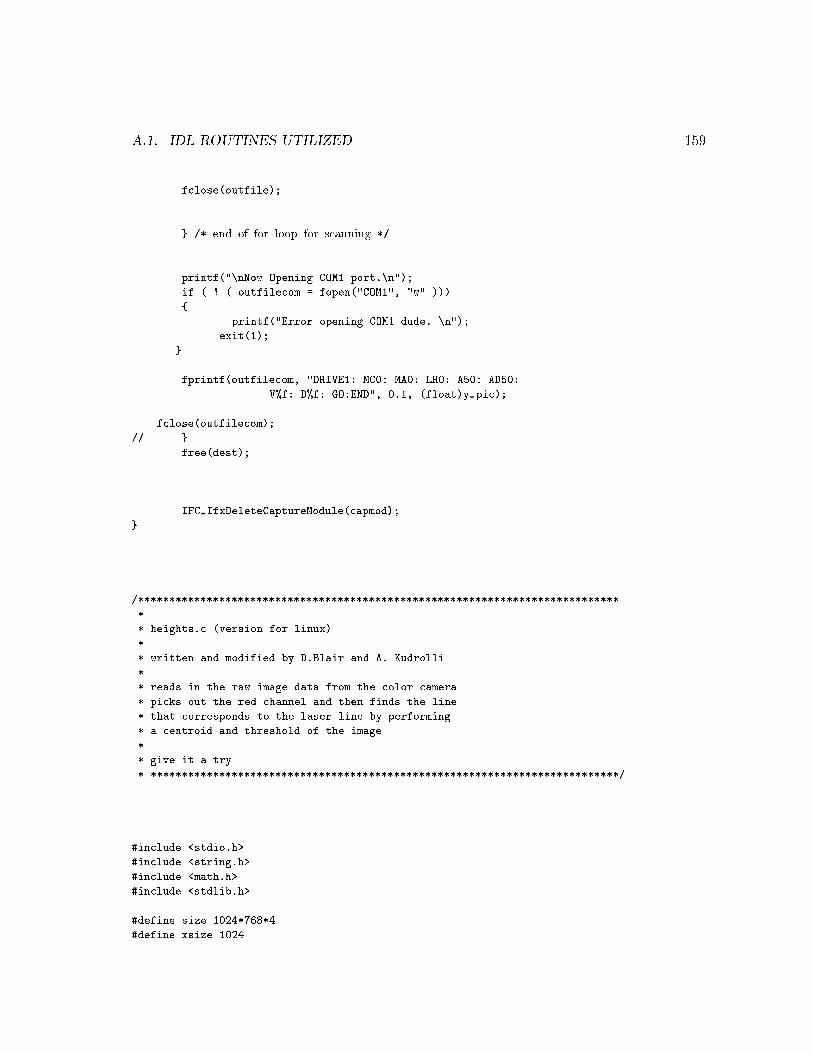
A.1. IDL ROUTINES UTILIZED 159f lose(outfile);} /* end of for loop for s anning */printf("\nNow Opening COM1 port.\n");if ( ! ( outfile om = fopen("COM1", "w" ))){ printf("Error opening COM1 dude. \n");exit(1);}fprintf(outfile om, "DRIVE1: MC0: MA0: LH0: A50: AD50:V%f: D%f: GO:END", 0.1, (float)y pi );f lose(outfile om);// }free(dest);IFC IfxDeleteCaptureModule( apmod);}/******************************************************************************* heights. (version for linux)** written and modified by D.Blair and A. Kudrolli** reads in the raw image data from the olor amera* pi ks out the red hannel and then finds the line* that orresponds to the laser line by performing* a entroid and threshold of the image** give it a try* ***************************************************************************/#in lude <stdio.h>#in lude <string.h>#in lude <math.h>#in lude <stdlib.h>#define size 1024*768*4#define xsize 1024

160 APPENDIX A. IDL AND C ROUTINES#define ysize 768#define ontrast 10*10#define half width 8FILE *infile, *outfile, *imgfile;int i, j, ount, n, data[xsize℄, thres[xsize℄, ii, temp;int Psi[xsize℄[ysize℄, diff, diff, image number;float ht[xsize℄, norm;int nread;//unsigned har buf[SIZE℄,//size t nread;unsigned har imgdata[size℄;unsigned har newimg[1024 * 768℄;main (){ har fnam1[95℄, fname[95℄, out name[95℄;//printf("%s", "image number: ");//s anf("%d", &image number);int n pi s = 2700;for (ii = 0; ii < n pi s; ii++){ image number = ii;// hange this to the dire tory where the data issprintf (fnam1, "/raid/blair/ rumple/ alibrate/ al5/test %5.5d.raw",image number);//printf("Now Opening in file. %s\n", fnam1);if (!(infile = fopen (fnam1, "rb"))){ printf ("Error opening input file. %s\n", fnam1);exit (1);}// this is the output file formsprintf (fname, "/raid/blair/ rumple/ alibrate/ al5/heights/t-%4.4d.dat",image number);printf ("Now Opening out file. %s\n", fname);if (!(outfile = fopen (fname, "w"))){ printf ("Error opening output file.%s\n", fname);exit (1);}//read the image datanread = fread ((void *) imgdata, 1, (size t) size, infile);for (i = 0; i < ysize; i++){for (j = 0; j < xsize; j++){

A.1. IDL ROUTINES UTILIZED 161int ij = ((i * xsize + j) * 4) + 2;Psi[j℄[i℄ = (int) imgdata[ij℄;}}temp = 0;for (i = 0; i < xsize; i++){ ount = 0; // sets ount to 0 for every ifor (j = 0; j < ysize; j++) // runs from the o�set value{ //di�eren e in every xth pixel spe i�ed by o�setif ((Psi[i℄[j℄ > temp)){ temp = Psi[i℄[j℄;//printf("%d\n",temp);data[i℄ = j;}}temp = 0;}//thresholdingfor (i = 0; i < xsize; i++)if (data[i℄ > 0) //ignore the x pixels with no y values{ thres[i℄ = 0;for (j = 0; j < ysize; j++){ thres[i℄ = thres[i℄ + Psi[i℄[j℄;}thres[i℄ = (int) (thres[i℄ / (float) ysize);norm = 0; // perform the entroidfor (j = -half width; j < half width + 1; j++){ ht[i℄ =ht[i℄ + (data[i℄ + j) * (Psi[i℄[(data[i℄ + j)℄ - thres[i℄);norm = norm + (Psi[i℄[(data[i℄ + j)℄ - thres[i℄);}fprintf (outfile, "%f\t%f\n", (float) i, ht[i℄ / (norm));ht[i℄ = 0.0;}f lose (infile); // lose �le img-*.dat

162 APPENDIX A. IDL AND C ROUTINESf lose (outfile); // lose �le img-*.new}return 0;}
BIBLIOGRAPHY 163Bibliography[1℄ Details of the monetary osts of grain use an be found at<http://widget.e n.purdue.edu/ psl/ba kground/mena>.[2℄ A tutorial for the IDL parti le tra king routines an be foundat <http://glinda.lrsm.upenn.edu/~weeks/idl>.[3℄ The FFTW (fastest Fourier transform in the west) website is<http://www.fftw.org/>.[4℄ For informaiton on the David Sarno� laboratory visit the website below<http://www.davidsarnoff.org/news.htm>.[5℄ B. J. A kerson and K. S h�atzel, Classi al growth of hard-sphere olloidal rystals,Phys. Rev. E 52, 6448 (1995).[6℄ M. Adams, Z. Dogi , S. L. Keller, and S. Fraden, Entropi ally driven mi rophasetransitions in mixtures of olloidal rods and spheres, Nature 393, 349 (1998).[7℄ B. J. Alder and T. E. Wainwright, Velo ity auto orrelations for hard spheres, Phys.Rev. Lett. 18, 988 (1967).[8℄ M. P. Allen and D. J. Tildesley, Computer Simulation of Liquids (Oxford, OxfordUniversity Press, 1996).[9℄ M. Ammi, D. Bideau, and J. P. Troade , Geometri al stru ture of disordered pa kingsof regular polygons; omparison with dis pa kings stru tures, J. Phys. D 20, 424(1987).[10℄ I. Aranson, D. Blair, W. Kwok, U. Welp, G. W. Crabtree, V. Vinokur, , and L. S.Tsimring, ` ontrolled dynami s of interfa es in a vibrated granular layer, Phys. Rev.Lett. 82, 731 (1999).[11℄ I. S. Aranson, D. Blair, V. A. Kalatsky, G. W. Crabtree, W.-K. Kwok, V. M. Vi-nokur, and U. Welp, Ele trostati ally driven granular media: Phase transitions and oarsening, Phys. Rev. Lett. 84, 3306 (2000).
164 BIBLIOGRAPHY[12℄ I. S. Aranson and L. Kramer, The world of the omplex ginzburg-landau equation,Rev. Mod. Phys. 74, 99 (2002).[13℄ I. S. Aranson, B. Meerson, P. V. Sasorov, and V. M. Vinokur, Phase separation and oarsening in ele trostati ally driven granular media, Phys. Rev. Lett. 88(20), 204301(2002).[14℄ I. S. Aranson and L. S. Tsimring, Formation of periodi and lo alized patterns in anos illating granular layer, Physi a A 249, 103 (1998).[15℄ M. Argentina, M. G. Cler , and R. Soto, van der waals-like transition in uidizedgranular matter, Phys. Rev. Lett. 89, 044301 (2002).[16℄ D. Astumian, Thermodynami s and kineti s of a brownian motor, S ien e 276, 632(1997).[17℄ E. Azanza, F. Chevoir, and P. Mou heront, Experimental study of ollisional granular ows down an in lined plane, J. Fluid Me h. 400, 199 (1999).[18℄ P. Bak, C. Tang, and K. Wiesenfeld, Self-organized riti ality: An explanation of 1/fnoise, Phys. Rev. Lett. 59, 381 (1987).[19℄ A. Baldassarri, U. M. B. Mar oni, A. Puglisi, and A. Vulpiani, Driven granular gaseswith gravity, Phys. Rev. E 64, 011301 (2001).[20℄ A. Barrat and E. Triza , Mole ular dynami s simulations of vibrated granular gases,Phys. Rev. E 66, 051303 (2002).[21℄ A. Barrat and E. Triza , Random inelasti ity and velo ity u tuations in a drivengranular gas, ond-mat/0205546 (2002).[22℄ G. W. Baxter, R. P. Behringer, T. Fagert, and G. A. Johnson, Pattern formation in owing sand, Phys. Rev. Lett. 62, 2825 (1989).[23℄ M. Z. Bazant, Statisti al dynami s of granular drainage, ond-mat/0307379 (2003).[24℄ G. A. Bird, Mole ular gas dynami s (Clarendon Press, Oxford, 1976).[25℄ G. A. Bird,Mole ular gas dynami s and the dire t simulation of gas ows (Clarendon,Oxford, 1994).[26℄ C. Bizon, Simulations of wave patterns in os illated granular media, Ph.D. thesis,University of Texas, Austin (1998).[27℄ C. Bizon, M. D. Shattu k, J. R. de Bruyn, J. B. Swift, W. D. M Cormi k, and H. L.Swinney, Conve tion and di�usion in patterns in os illated granular media, J. Stat.Phys. 93(3/4), 449 (1998).

BIBLIOGRAPHY 165[28℄ C. Bizon, M. D. Shattu k, and J. B. Swift, Linear stability analysis of a verti allyos illated granular layer, Phys. Rev. E 60, 7210 (1999).[29℄ C. Bizon, M. D. Shattu k, J. B. Swift, W. D. M Cormi k, and H. L. Swinney, Patternsin 3d verti ally os illated granular layers: Simulation and experiment, Phys. Rev. Lett.80(1), 57 (1998).[30℄ C. Bizon, M. D. Shattu k, J. B. Swift, and H. L. Swinney, Transport oeÆ ients forgranular media from mole ular dynami s simulations, Phys. Rev. E 60, 4340 (1999).[31℄ C. Bizon, M. D. Shattu k, J. B. Swift, and H. L. Swinney, Velo ity orrelationsin driven two-dimensional granular media, in J. Karkhe k, editor, Dynami s: Modelsand Kineti Methods for Nonequilibrium Many-Body Systems, pages 361{371 (KluwerA ademi Publishers, Dordre ht, 2000), ond-mat/9904135.[32℄ D. Blair, I. Aranson, G. W. Crabtree, V. Vinokur, L. S. Tsimring, and C. Josserand,Patterns in thin vibrated granular layers: Interfa es, hexagons, and superos illons 61,5600 (2000).[33℄ D. Blair and A. Kudrolli, Clustering transitions in vibro- uidized magnetized granularmaterials, Phys. Rev. E 67, 021302 (2003).[34℄ D. L. Blair and A. Kudrolli, Velo ity orrelations in dense granular gases, Phys. Rev.E 64, 050301 (2001).[35℄ D. L. Blair and A. Kudrolli, Collision statisti s of driven granular materials, Phys.Rev. E 67, 041301 (2003).[36℄ D. L. Blair, N. W. Mueggenburg, A. H. Marshall, H. M. Jaeger, and S. R. Nagel,For e distributions in three-dimensional granular assemblies: E�e ts of pa king orderand inter-parti le fri tion, Phys. Rev. E 63, 041304 (2001).[37℄ D. L. Blair, T. Nei u, and A. Kudrolli, Vorti es in vibrated granular rods, Phys. Rev. E67, 031303 (2003).[38℄ L. Boltzmann, Further studies on the thermal equilibrium among gas-mole ules,Wien.Ber. 66, 275 (1872).[39℄ A. Boudaoud, P. Patr�� io, Y. Couder, and M. B. Amar, Dynami s of singulartities ina onstrined elasti plate, Nature 407, 718 (2000).[40℄ J. J. Brey and M. J. Ruiz-Montero, Velo ity distribution of uidized granular gasesin the presen e of gravity, Phys. Rev. E 67, 021307 (2003).[41℄ J. J. Brey, M. J. Ruiz-Montero, R. Gar ��a-Rojo, and J. W. Dufty, Brownian motionin a granular gas, Phys. Rev. E 60, 7174 (1999).

166 BIBLIOGRAPHY[42℄ K. Butter, P. H. H. Bomans, P. M. Frederik, G. J. Vroege, and A. P. Philipse, Dire tobservation of dipolar hains in iron ferro uids by ryogeni ele tron mi ros opy,Nature Materials 2, 88 (2003).[43℄ S. H. C.-K. Peng, H. Stanley, and A. Goldberger, Quanti� ation of s aling exponentsand rossover phenomena in nonstationary heartbeat time series, Chaos 5, 82 (1995).[44℄ P. J. Camp, J. C. Shelley, and G. N. Patey, Isotropi uid phases of dipolar hardspheres, Phys. Rev. Lett. 84, 115 (2002).[45℄ N. F. Carnahan and K. E. Starling, Equation of state for nonattra ting ridged spheres,J. Chem. Phys. 51(2), 635 (1969).[46℄ E. Cerda, S. Chaieb, F. Melo, and L. Mahadevan, Coni al dislo ations in rumpling,Nature 401, 46 (1999).[47℄ E. Cerda and L. Mahadevan, Geometry and Physi s of Wrinkling, Phys. Rev. Lett.90, 074302 (2003).[48℄ E. Cerda and L. Mahadeven, Coni al surfa es and resent singularities in rumpledsheets, Phys. Rev. Lett. 80, 2358 (1998).[49℄ E. Cerda, K. Ravi-Shankar, and L. Mahadevan, Wrinkling in an elasti sheet undertension, Nature 53, 579 (2002).[50℄ S. Cha��eb and F. Melo, Experimental study of rease formation in an axially om-pressed sheet .[51℄ S. Cha��eb and F. Melo, Cresent singularities and stress fo using in a bu kled thinsheet: Me hani s and developable ones, Phys. Rev. E 60, 6091 (1999).[52℄ S. Cha��eb, F. Melo, and J.-C. G�eminard, Experimental study of developable ones,Phys. Rev. Lett. 80, 2354 (1998).[53℄ P. M. Chaikin and T. C. Lubinksy, Prin iples of Condensed Matter Physi s (Cam-bridge, Cambridge University Press, 1995).[54℄ D. Chandler, J. D. Weeks, and H. C. Anderson, he van der waals pi ture of liquids,solids and phase transformations, S ien e 220, 787 (1983).[55℄ S. Chapman and T. G. Cowling, The Mathemati al Theory of Non-Uniform Gases(Cambridge, Cambridge University Press, 1970).[56℄ F. Chladni, Die Akustik (Leipzig Breitkopf & H�artel, Leipzig, 1802).[57℄ J. Choi, A. Kudrolli, R. R. Rosales, and M. Z. Bazant, Di�usion and mixing ingravity-driven dense granular ows.

BIBLIOGRAPHY 167[58℄ E. Cl�ement and L. Labous, Pattern formation in a vibrated granular layer: Thepattern sele tion issue, Phys. Rev. E 62, 8314 (2000).[59℄ E. Cl�ement, L. Vanel, J. Raj henba h, and J. Duran, Pattern formation in a vibratedgranular layer, Phys Rev. E 53(3), 2972 (1996).[60℄ S. N. Coppersmith, C. Liu, s. Majumdar, O. Narayan, and T. A. Witten, Model forfor e u tuations in bead pa ks, Phys. Rev. E 53, 4673 (1996).[61℄ C. A. Coulomb, A ad. R. S i. Mem. Math. Phys. par Divers Savants 7, 343 (1773).[62℄ C. Crawford and H. Rie ke, Os illon-type stru tures and their intera tion in a swift-hohenberg model, Physi a D 129, 83 (1999).[63℄ J. C. Cro ker and D. G. Grier, Methods of digital video mi ros opy for olloidalstudies, J. Colloid Interfa e S i. 197, 298 (1996).[64℄ M. C. Cross and P. C. Hohenberg, Pattern formation outside of equilibrium, Rev.Mod. Phys. 65, 851 (1993).[65℄ P. K. Das and D. Blair, Phase boundaries in verti ally vibrated granular materials,Phys. Lett. A 242, 7953 (1998).[66℄ P. G. de Gennes, Re e tions on the me hani s of granular matter, Physi a A 261,267 (1998).[67℄ P. G. de Gennes, Granular matter: a tentative view, Rev. Mod. Phys. 71, S374 (1999).[68℄ P. G. deGennes and P. A. Pin us, Pair orrelations in a ferromagneti olloid,Phys. Kondens. Mater. 11, 189 (1970).[69℄ B. A. DiDonna, S aling of the bu kling transition of ridges in thin sheets, Phys. Rev.E 66, 016601 (2002).[70℄ B. A. DiDonna and T. A. Witten, Anomalous Strength of Membranes with Elasti Ridges, Phys. Rev. Lett. 87, 206105 (2001).[71℄ F. Dinkela ker, A. H�ubler, and E. L�us her, Pattern formation of powder on a vibratingdis , Biol. Cybern. 56, 51 (1987).[72℄ C. C. Donto, M. A. Gomes, and R. E. de Souza, S aling properties in the pa king of rumpled wires, Phys. Rev. E 67, 026110 (2003).[73℄ S. Douady, S. Fauve, and C. Laro he, Subharmoni instabilities and defe ts in agranular layer under verti al vibrations, Europhys. Lett. 8(7), 621 (1989).[74℄ Y. Du, H. Li, and L. P. Kadano�, Breakdown of hydrodynami s in a one-dimensionalsystem of inelasti parti les, Phys. Rev. Lett. 74(8), 1268 (1995).
168 BIBLIOGRAPHY[75℄ M. D. S. E. C. Reri ha, C. Bizon and H. L. Swinney, Sho ks in supersoni sand, Phys.Rev. Lett. 88, 014302 (2002).[76℄ J. Eggers, Sand as Maxwell's demon, Phys. Rev. Lett. 83, 5322, ond-mat/9906275(1999).[77℄ J. Eggers and H. Rie ke, Continuum des ription of vibrated sand, Phys. Rev. E 59(4),4476, patt-sol/9801004 (1999).[78℄ E. E. Ehri hs, H. M. Jaeger, G. S. Kar zmar, J. B. Knight, V. Kuperman, and S. R.Nagel, Granular onve tion observed by magneti resonan e imaging, S ien e 267,1632 (1995).[79℄ E. Fal on, C. Laro he, S. Fauve, and C. Coste, Behavior of one inelasti ball boun ingrepeatedly o� the ground, Eur. Phys. J. B 3, 45 (1998).[80℄ M. Faraday, On a pe uliar lass of a ousti al �gures; and on ertain forms assumedby groups of parti les upon vibrating elasti surfa es, Philos. Trans. R. So . London52, 299 (1831).[81℄ K. Fetosa and N. Menon, Breakdown of energy equipartition in a 2d binary vibratedgranular gas, Phys. Rev. Lett. 88, 198301 (2002).[82℄ R. P. Feynman, The Feynman Le tures on Physi s, volume 2 (1995).[83℄ A. J. Forsyth, S. R. Hutton, C. F. Osborne, and M. J. Rhodes, E�e ts of interparti lefor e on the pa king of spheri al granular material, Phys. Rev. Lett. 87, 244301 (2001).[84℄ Y. Forterre and O. Pouliquen, Longitudinal vorti es in granular ows, Phys. Rev.Lett. 86, 5886 (2001).[85℄ U. Gasser, E. R. Weeks, A. S. S ho�eld, P. N. Pusey, and D. A. Weitz, Real spa eimaging of nu leation and growth in olloidal rystallization, S ien e 292, 258 (2001).[86℄ I. Goldhirs h, M.-L. Tan, and G. Zanetti, A mole ular dynami s study of granular uids i: The unfor ed granular gas in two dimensions, J. S ient. Comp. 8, 1 (1993).[87℄ I. Goldhirs h and G. Zanetti, Clustering instability in dissipative gases, Phys. Rev.Lett. 70(11), 1619 (1993).[88℄ A. Goldshtein, M. Shapiro, L. Moldavsky, and M. Fi hman, Me hani s of ollisionalmotion of granular materials. Part 2. Wave propagation through vibro uidized gran-ular layers, J. Fluid Me h. 287, 349 (1995).[89℄ M. A. Gomes, T. I. Jyh, I. M. Rodrigues, and C. B. S. Furtado, Me hani ally deformed rumpled surfa es, J. Phys. D: Appl. Phys. 22, 1217 (1989).
BIBLIOGRAPHY 169[90℄ M. A. F. Gomes, Paper rushes fra tally, Journal of Physi s A Mathemati al General20, L283 (1987).[91℄ M. A. F. Gomes, T. I. Jyh, and T. I. Ren, The rumpled state of some non-equilibriumfra tal surfa es, Journal of Physi s A Mathemati al General 23, L1281 (1990).[92℄ P. Grassberger and I. Pro a ia, Chara terization of strange attra tors,Phys. Rev. Lett. 50, 346 (1983).[93℄ E. L. Grossman, T. Zhou, and E. Ben-Naim, owards granular hydrodynami s in twodimensions, Phys. Rev. E 55, 4200 (1997).[94℄ C. h. Liu, S. R. Nagel, D. A. S he ter, S. N. Coppersmith, S. Majumdar, O. Narayan,and T. A. Witten, For e u tuations in bead pa ks, S ien e 269, 513 (1995).[95℄ P. K. Ha�, Grain ow as a uid-me hani al phenomenon, J. Fluid Me h. 134, 401(1983).[96℄ H. Hayakawa and D. C. Hong, Thermodynami theory of weakly ex ited granularsystems, Phys. Rev. Lett. 78(14), 2764 (1997).[97℄ C. E. He ht, Statisti al Thermodynami s and Kineti Theory (Dover, Dover Publi a-tions New York, 1998).[98℄ D. Helbing and M. Treiber, Gas-kineti -based traÆ model explaining observed hys-tereti phase transition, Phys. Rev. Lett. 81, 3042 (1998).[99℄ D. Henderson, Mole . Phys. 30, 971 (1975).[100℄ D. J. Hornbaker, R. Albert, I. Albert, A. L. Barabsi, and P. S hi�er, What keepssand astles standing?, Nature 387, 765 (1997).[101℄ J. Hoshen and R. Kopelman, Per olation and luster distribution. i. luster multiplelabeling te hnique and riti al on entration algorithm, Phys. Rev. B 14, 3438 (1976).[102℄ P. A. Houle and J. P. Sethna, A ousti emission from rumpling paper, Phys. Rev. E54, 278 (1996).[103℄ D. Howell, C. T. Veje, and R. Behringer, Stress u tuations in a 2d granular ouetteexperiment: A riti al transition, Phys. Rev. Lett. 82, 5241 (1999).[104℄ D. W. Howell, Stress Distributions and Flu tuations in Stati and Quasi-stati Gran-ular Systems, Ph.D. thesis, Duke University, Department of Physi s (1999).[105℄ D. W. Howell, I. S. Aranson, and G. W. Crabtree, Dynami s of ele trostati ally-drivengranular media: E�e ts of humidity., Phys. Rev. E 63(5), 1315 (2001).[106℄ D. W. Howell, I. S. Aronson, and G. W. Crabtree, Dynami s of ele trostati ally drivengranular media: E�e ts of humidity, Phys. Rev. E 63, 050301(R) (2001).

170 BIBLIOGRAPHY[107℄ D. W. Howell, R. P. Behringer, and C. T. Veje, Flu tuations in granular media, Chaos9(3), 559 (1999).[108℄ H. M. Jaeger, C. h. Liu, and S. R. Nagel, Relaxation at the angle of repose, Phys.Rev. Lett. 62, 40 (1989).[109℄ H. M. Jaeger, C. h. Liu, and S. R. Nagel, Relaxation at the angle of repose, Phys.Rev. Lett. 62, 40 (1989).[110℄ H. M. Jaeger, S. R. Nagel, and R. P. Behringer, Granular solids, liquids, and gases,Rev. Mod. Phys. 68, 1259 (1996).[111℄ H. A. Janssen, Versu he �uber Getreidedru k in silozellen, Zeits hr. d. Vereinesdeut her Ingenieure 39, 1045 (1895).[112℄ J. T. Jenkins and M. W. Ri hman, Kineti theory for plane shear ows of a dense gasof identi al, rough, inelasti , ir ular disks, Phys. of Fluids 28, 3485 (1985).[113℄ J. T. Jenkins and R. W. Ri hman, Grad's 13-moment system for a dense gas ofinelasti spheres, Ar h. Rat. Me h. Anal. 87, 355 (1985).[114℄ J. T. Jenkins and S. B. Savage, A theory for the rapid ow of identi al, smooth, nearlyelasti , spheri al parti les, J. Fluid Me h. 130, 187 (1983).[115℄ J. T. Jenkins and M. Shahinpoor, Ma ros opi phase transitions in two-dimensionalgranular materials, in J. T. Jenkins and M. Satake, editors, Me hani s of GranularMaterials: New Models and Constitutive Relations, pages 339{346 (Elsevier, Amster-dam, 1983).[116℄ L. P. Kadano�, Built upon sand: Theoreti al ideas inspired by granular ows, Rev.Mod. Phys. 71, 435 (1999).[117℄ Y. Kantor, M. Kardar, and D. R. Nelson, Statisti al me hani s of tethered surfa es,Phys. Rev. Lett. 57, 791 (1986).[118℄ P. D. Kaplan, J. L. Rouke, A. G. Yodh, and D. J. Pine, Entropi ally driven surfa ephase separation in binary olloidal mixtures, Phys. Rev. Lett. 72, 582 (1994).[119℄ W. Kauzmann, Kineti Theory of Gases. (Benjamin, New York, 1966).[120℄ E. Khain and B. Meerson, Symmetry-breaking instability in a prototypi al drivengranular gas, Phys. Rev. E 66, 021306 (2002).[121℄ C. Kittel, Solid State Physi s (Cambridge, Cambridge University Press, 1997).[122℄ J. B. Knight, External boundaries and internal shear bands in granular onve iton,Phys. Rev. E 55(5), 6016 (1997).

BIBLIOGRAPHY 171[123℄ J. B. Knight, E. E. Ehri hs, V. Kuperman, J. K. Flint, H. M. Jaeger, and S. R. Nagel,Experimental study of granular onve tion, Phys. Rev. E 54(5), 5726 (1996).[124℄ J. B. Knight, C. G. Fandri h, C. N. Lau, H. M. Jaeger, and S. R. Nagel, Densityrelaxation in a vibrated granular material, Phys. Rev. E 51(5), 3957 (1995).[125℄ J. B. Knight, H. M. Jaeger, and S. R. Nagel, Vibration-indu ed size separation ingranular media: The onve tion onne tion, Phys. Rev. Lett. 70(24), 3728 (1993).[126℄ L. Kondi , Dynami s of spheri al parti les on a surfa e: Collision-indu ed sliding andother e�e ts, Phys. Rev. E 60, 751 (1999).[127℄ E. M. Kramer and A. E. Lobkovsky, Universal power law in the noise from a rumpledelasti sheet, Phys. Rev. E 53, 1465 (1996).[128℄ E. M. Kramer and T. A. Witten, Stress ondensation in rushed elasti manifolds,Phys. Rev. Lett. 78, 1303 (1997).[129℄ A. Kudrolli and J. Henry, Non-gaussian velo ity distributions in ex ited granularmatter in the absen e of lustering, Phys. Rev. E 62, R1489 (2000).[130℄ A. Kudrolli, M. Wolpert, and J. P. Gollub, Cluster formation due to ollisions ingranular material, Phys. Rev. Lett. 78, 1383 (1997).[131℄ V. Kumaran, Temperature of a granular material \ uidized" by external vibrations,Phys. Rev. E 57(5), 5660 (1998).[132℄ V. Kumaran, Velo ity distribution for a dilute vibrated granular material, Phys. Rev.E 59(4), 4188 (1999).[133℄ L. Landau and E. Lifshitz, Theory of Elasti ity (Pergamon, Oxford, 1986).[134℄ Y. Levin, hat happened to the gas-liquid transition in the system of dipolar hardspheres?, Phys. Rev. Lett. 83, 1159 (1999).[135℄ J. Li, I. S. Aranson, W.-K. Kwok, and L. S. Tsimring, Periodi and disordered stru -tures in a modulated gas driven granular layer, Phys. Rev. Lett. 90, 134301 (2003).[136℄ P. Linse and V. Lobaskin, Ele trostati attra tion and phase separation in solutionsof like- harged olloidal parti les, Phys. Rev. Lett. 83, 4208 (1999).[137℄ A. J. Liu and S. R. Nagel, Nonlinear dynami s: Jamming is not just ool any more,Nature 396, 21 (1998).[138℄ E. Livne, B. Meerson, and P. V. Sasorov, Symmetry-breaking instability and stronglypeaked periodi lustering states in a driven granular gas, Phys. Rev. E 65, 021302(2002).

172 BIBLIOGRAPHY[139℄ A. E. Lobkovsky, S. Gentges, H. Li, D. Morse, and T. A. Witten, S aling propertiesof stret hing ridges in a rumpled elasti sheet, S ien e 270, 1482 (1995).[140℄ A. E. Lobkovsky and T. A. Witten, Properties of ridges in elasti membranes, Phys.Rev. E 55, 1577 (1997).[141℄ W. Losert, D. Copper, J. Delour, A. Kudrolli, and J. P. Gollub, Velo ity statisti s invibrated granular media, Chaos 9, 682 (1999).[142℄ S. Luding, E. Cl�ement, A. Blumen, J. Raj henba h, and J. Duran, Studies of olumnsof beads under external vibrations, Phys. Rev. E 49, 1634 (1994).[143℄ H. Mamiya, I. Nakatani, and T. Furubayashi, Phase transitions of iron-nitride mag-neti uids, Phys. Rev. Lett. 84, 6106 (2000).[144℄ K. Matan, R. B. Williams, T. A. Witten, and S. R. Nagel, Crumpling a thin sheet,Phys. Rev. Lett. 88, 076101 (2002).[145℄ J. C. Maxwell, On the vis osity or internal fri tion of air and other gases,Phil. Trans. Roy. So . 157, 49 (1866).[146℄ S. M Namara and S. Luding, Energy ows in vibrated granular media, Phys. Rev. E58, 813 (1998).[147℄ S. M Namara and S. Luding, Energy nonequipartition in systems of inelasti , roughspheres, Phys. Rev. E 58, 2247 (1998).[148℄ S. M Namara and W. R. Young, Inelasti ollapse and lumping in a one-dimensionalgranular medium, Phys. Fluids A 4, 496 (1992).[149℄ S. M Namara and W. R. Young, Dynami s of a freely evolving, two-dimensionalgranular medium, Phys. Rev. E 53, 5089 (1996).[150℄ F. Melo, P. B. Umbanhowar, and H. L. Swinney, Transition to parametri wave pat-terns in a verti ally os illated granular layer, Phys. Rev. Lett. 72(1), 172 (1994).[151℄ F. Melo, P. B. Umbanhowar, and H. L. Swinney, Hexagons, kinks, and disorder inos illated granular layers, Phys. Rev. Lett. 75(21), 3838 (1995).[152℄ N. Menon and D. J. Durian, Parti le motions in a gas- uidized bed of sand, Phys.Rev. Lett. 79, 3407 (1997).[153℄ A. Metha and J. M. Lu k, Novel temporal behavior of a nonlinear dynami al system:The ompletely inelasti boun ing ball, Phys. Rev. Lett. 65, 393 (1990).[154℄ S. J. Moon, M. D. Shattu k, C. Bizon, D. I. Goldman, J. B. Swift, and H. L. Swin-ney, Phase bubbles and spatiotemporal haos in granular patterns, Phys. Rev. E 65,011301 (2002).

BIBLIOGRAPHY 173[155℄ S. J. Moon, M. D. Shattu k, and J. B. Swift, Velo ity distributions and orrelationsin homogeneously heated granular media, Phys. Rev. E 64, 031303 (2001).[156℄ G. E. Moore, Cramming more omponents onto integrated ir uits, Ele troni s 38(1965).[157℄ W. A. M. Morgado and E. R. Mu iolo, ond-mat/0204084, Physi a A to appear.[158℄ S. W. Morris, E. Bodens hatz, D. S. Cannell, and G. Ahlers, Spiral defe t haos inlarge aspe t ratio rayleigh-b�eynard onve tion, Phys. Rev. Lett. 71, 2026 (1993).[159℄ C. C. Moun�eld and S. F. Edwards, A theoreti al model for the stress distribution ingranular matter, Physi a A 210, 279 (1994).[160℄ D. M. Mueth, G. F. Debregeas, G. S. Kar zmar, P. J. Eng, S. R. Nagel, and H. M.Jaeger, Signatures of granular mi rostru ture in dense shear ows, Nature 406, 385(2000).[161℄ D. M. Mueth, H. M. Jaeger, and S. R. Nagel, For e distributions in a granular medium,Phys. Rev. E. 57, 3164 (1998).[162℄ R. Mukhopadhyay, G. Lim, and M. Wortis, E hino yte shapes: Bending, stret hing,and shear determine spi ule shape and spa ing, Biophys. J. 82, 1756 (2002).[163℄ S. Nagel, Instabilities in a sandpile, Rev. Mod. Phys. 64, 321 (1992).[164℄ R. Nedderman, Stati s and Kinemati s of Granular Materials (Cambridge UniversityPress, 1991).[165℄ D. Nelson, T. Piran, and S. Weinberg, Statisti al me hani s of membranes and sur-fa es (World S ienti� , Singapore, 1988).[166℄ S. Ogawa, Multitemperature theory of granular materials, in Pro . US - Japan Semin.Contin-Me h. and Stat. Approa hes Me h. Granular Mater , page 208 (GukujustuBunken Fukyakai, Tokyo, 1978).[167℄ J. S. Olafsen and J. S. Urba h, Clustering, order, and ollapse in a driven granularmonolayer, Phys. Rev. Lett. 81, 4369 (1998).[168℄ J. S. Olafsen and J. S. Urba h, Velo ity distributions and density u tuations in agranular gas, Phys. Rev. E 60, R2468 (1999).[169℄ L. Onsager, The e�e ts of shape on the intera tion of olloidal parti les., Ann. NYA ad. S i. 51, 627 (1949).[170℄ I. Pagonabarraga, E. Triza , T. P. C. van Noije, and M. H. Ernst, Randomly drivengranular uids: Collisional statisti s and short s ale stru ture, Phys. Rev. E 65,011303 (2002).

174 BIBLIOGRAPHY[171℄ H. K. Pak and P. R. Behringer, Bubbling in verti ally vibrated granular materials,Nature 371, 231 (1994).[172℄ H. K. Pak and R. P. Behringer, Surfa e waves in verti ally vibrated granular materials,Phys. Rev. Lett. 71(12), 1832 (1993).[173℄ D. Paolotti, C. Cattuto, U. M. B. Mar oni, and A. Puglisi, Dynami al properties ofvibro uidized granular mixtures, ond-mat/0207601 (2002).[174℄ G. Peng and T. Ohta, Steady state properties of a driven granular medium, Phys.Rev. E 58, 4737 (1999).[175℄ F. Plourabou�e and S. Roux, Experiemntal study of the roughness of rumpled sheets,Physi a A 227, 173 (1996).[176℄ O. Pouliquen, S aling laws in granular ows down rough in lined planes (1998).[177℄ O. Pouliquen, On the shape of granular fronts down rough in lined planes (1999).[178℄ O. Pouliquen, J. Delour, and S. B. Savage, Fingering in granular ows, Letters toNature 386, 816 (1997).[179℄ O. Pouliquen and R. Gutfraind, Stress u tuations and shear zones in quasi-stati granular hute ows, Phys. Rev. E 53(1), 552 (1996).[180℄ O. Pouliquen, M. Ni olas, and P. Weidman, Crystallization of non-brownian spheresunder horizontal shaking (1997).[181℄ O. Pouliquen and N. Renaut, Onset of granular ows on an in lined rough bed:dilatan y e�e ts, J. Ohys. II (Fran e) 6, 923 (1996).[182℄ A. Prevost, D. A. Egolf, and J. S. Urba h, For ing and velo ity orrelations in avibrated granular monolayer, Phys. Rev. Lett. 89, 084301 (2002).[183℄ A. Prevost, D. A. Egolf, and J. S. Urba h, For ing and velo ity orrelations in avibrated granular monolayer, Phys. Rev. Lett. 89, 084301 (2002).[184℄ A. Puglisi, V. Loreto, U. M. B. Mar oni, A. Petri, and A. Vulpiani, Clustering andnon-gaussian behavior in granular matter, Phys. Rev. Lett. 81, 3848 (1998).[185℄ A. Puglisi, V. Loreto, U. M. B. Mar oni, and A. Vulpiani, Kineti approa h to granulargases, Phys. Rev. E 59, 5582 (1999).[186℄ R. Ram��rez and R. Soto, Temperature inversion in granular uids under gravity, ond-mat/0210471 (2002).[187℄ F. Reif, Statisti al Me hani s (M Graw-Hill, New York).

BIBLIOGRAPHY 175[188℄ O. Reynolds, On the dilaten y of media omposed of ridged parti les in onta t,Philos. Mag. Ser. 5, 50 (1885).[189℄ G. H. Ristow, Pattern formation in granular matter (Springer-Verlag, 2000).[190℄ R. E. Rosensweig, Ferrohydrodynami s (Cambridge, Cambridge University Press,1985).[191℄ D. H. Rothman, Os illons spiral waves and stripes in a model of vibrated sand (1999).[192℄ F. Rouyer and N. Menon, Velo ity u tuations in a homogeneous 2d granular gas insteady state, Phys. Rev. Lett. 85, 3676 (2000).[193℄ A. Samadani and A. Kudrolli, Segregation transitions in wet granular matter, phys.Rev. Lett. 85, 5102 (2000).[194℄ A. Samadani, L. Mahadevan, and A. Kudrolli, Sho ks in sand owing in a silo, J.Fluid Me h. 452, 293 (2002).[195℄ A. Samadani, A. Pradhan, and A. Kudrolli, Size segregation of granular matter insilo dis harges, Phys. Rev. E 60(6), 7203 (1999).[196℄ M. V. Sapozhnikov, Y. V. Tolma hev, I. S. Aranson, and W.-K. Kwok, Dynami self-assembly and patterns in ele trostati ally driven granular media, Phys. Rev. Lett. 90,114301 (2003).[197℄ S. B. Savage and M. Sayed, Stresses developed by dry ohesionless granular materialsin an annular ell, J. Fluid Me h. 142, 391 (1984).[198℄ N. S horghofer and T. Zhou, Inelasti ollapse of rotating spheres, Phys. Rev. E 54,5511 (1996).[199℄ R. P. Sear, Low-density uid phase of dipolar hard spheres, Phys. Rev. Lett. 76, 2310(1996).[200℄ J. P. Sethna, K. A. Dahmen, and C. R. Meyers, Cra kling noise, Nature 410, 242(2001).[201℄ E. Sharon, B. Roman, M. Marder, G.-S. Shin, and H. L. Swinney, Bu kling as adein free sheets, Nature 53, 579 (2002).[202℄ M. D. Shattu k, C. Bizon, P. B. Umbanhowar, J. B. Swift, and H. L. Swinney, 2dverti ally vibrated granular media: Experiment and simulation, in Powders & Grains97 (Balkema, Rotterdam, 1997).[203℄ T. Shinbrot, Competition between randomizing impa ts and inelasti ollisions ingranular pattern formation, Nature 389(6651), 574 (1997).

176 BIBLIOGRAPHY[204℄ R. Soto and M. Mares hal, Statisti al me hani s of uidized granular media: Short-range velo ity orrelations, Phys. Rev. E 63, 041303 (2001).[205℄ R. Soto, J. Piase ki, and M. Mares hal, Pre ollisional velo ity orrelations in a hard-disk uid with dissipative ollisions, Phys. Rev. E 64, 031306 (2001).[206℄ P. Sunthar and V. Kumaran, Temperature s aling in a dense vibro uidized granularmaterial, Phys. Rev. E 60, 1951 (1999).[207℄ S. Tazekas, J. Kertese, and D. Wolf, private ommuni ation.[208℄ P. Tegzes, T. Vi sek, and P. S hi�er, Development of orrelations in the dynami s ofwet granular avalan hes, Phys. Rev. E 67, 051303 (2003).[209℄ P. R. ten Wolde, D. W. Oxtoby, and D. Frenkel, Chain formation in homogeneousgas-liquid nu leation of polar uids,, J. Chem. Phys. 111, 4762 (1999).[210℄ D. Thompson, On Growth and Form (Cambridge University Press, 1917).[211℄ T. Tlusty and S. A. Safran, Defe t-indu ed phase separation in dipolar uids, S ien e290, 1328 (2000).[212℄ L. S. Tsimring and I. S. Aranson, Lo alized and ellular patterns in a vibrated granularlayer, Phys. Rev. Lett. 79, 213 (1997).[213℄ F. Tzs hi hholz, A. Hansen, and S. Roux, Roughness of randomly rumpled elasti sheets, ond-mat/9507056.[214℄ S. Ulam, On the operations of pair produ tion, transmutations and generalized ran-dom walk, Adv. Appl. Math 1, 7 (1980).[215℄ P. B. Umbanhowar, F. Melo, and H. L. Swinney, Lo alized ex itations in a verti allyvibrated granular layer, Nature 382, 793 (1996).[216℄ P. B. Umbanhowar and H. L. Swinney, Wavelength s aling and square/stripe and grainmobility transitions in verti ally os illated granular layers, nlin.PS/0001061 (2000).[217℄ D. van der Meer, P. Reimann, K. van der Weele, and D. Lohse, Spontaneous rat hete�e t in a granular gas, ont-matt/0306640.[218℄ D. van der Meer, K. van der Weele, and D. Lohse, Sudden ollapse of a granular luster, Phys. Rev. Lett. 88, 174302 (2002).[219℄ M. E. van Leeuwen and B. Smit, What makes a polar liquid a liquid?, Phys. Rev.Lett. 71, 3991 (1993).[220℄ T. P. C. van Noije and M. H. Ernst, Velo ity distributions in homogeneous granular uids: the free and the heated ase, Granular Matter 1, 57 (1998).

BIBLIOGRAPHY 177[221℄ T. P. C. van Noije, M. H. Ernst, E. Triza , and I. Pagonabarraga, Randomly drivengranular uids: Large-s ale stru ture, Phys. Rev. E 59, 4326 (1999).[222℄ R. van Roij, Theory of hain asso iation versus liquid ondensation, Phys. Rev. Lett.76, 3348 (1996).[223℄ J. S. van Zon and F. C. Ma Kintosh, Velo ity distributions in dilute granular systems, ond-mat/0205512 (2002).[224℄ L. Vanel, P. Claudin, J. P. Bou houd, M. E. Cates, E. Cl�ement, and J. P. Wittmer,Stresses in silos: Comparison between theoreti al models and new experiments, Phys.Rev. Lett. 84, 1439 (2000).[225℄ F. X. Villarruel, B. E. Lauderdale, D. M. Mueth, and H. M. Jaeger, Compa tion ofrods: Relaxation and ordering in vibrated, anisotropi granular material, Phys. Rev.E 61, 6914 (2000).[226℄ D. Volfson and L. S. Tsimring, Slipping sti ks: Mi ros opi des ription of vortexformation.[227℄ G. A. Voth, B. Bigger, M. R. Bu kley, W. Losert, M. P. Brenner, H. A. Stone, andJ. P. Gollub, Ordered lusters and dynami al states of parti les in a vibrated uid,Phys. Rev. Lett. 88, 234301 (2002).[228℄ R. M. Wald, General Relativity (University of Chi ago Press, 1984).[229℄ H. Wang, Y. Zhua, C. Boyd, W. Luo, A. Cebers, and R. E. Rosensweig, Periodi bran hed stru tures in a phase-separated magneti olloid, Phys. Rev. Lett. 72, 1929(1994).[230℄ S. Warr and J. M. Huntley, Energy input and s aling laws for a single parti le vibratingin one dimension, Phys. Rev. E 52, 5596 (1995).[231℄ S. Warr, J. M. Huntley, and G. T. H. Ja ques, Fluidization of a two-dimensionalgranular system: Experimental study and s aling behavior, Phys. Rev. E 52, 5583(1995).[232℄ S. Warr, G. T. H. Ja ques, and J. M. Huntley, Tra king the translational and rota-tional motion of granular parti le: use of high-speed photography and image pro ess-ing, Powder Te h. 81, 41 (1994).[233℄ W. Wen, F. Kun, K. F. P�al, D. W. Zheng, and K. N. Tu, Aggregation kineti s andstability of stru tures formed by magneti mi rospheres, Phys. Rev. E 59, R4758(1999).[234℄ C. Wetter, Die ussigkristalle des tabakmosaikvirus, Biologie in unserer Zeit 3, 81(1985).

178 BIBLIOGRAPHY[235℄ G. M. Whitesides and B. Grzybowski, Self-assembly at all s ales, S ien e 296, 2418(2002).[236℄ R. D. Wildman, J. M. Huntly, and J.-P. Hansen, Self-di�usion of grains in a two-dimensional vibro uidized bed, Phys. Rev. E 60, 7066 (1999).[237℄ A. J. Wood, Witten's le tures on rumpling, Physi a A 313, 83 (2002).[238℄ J. Wood, The geomorphologi al hara terisation of digital elevation models, Ph.D.thesis, University of Lei ester (1996).[239℄ X. Yang, C. Huan, D. Candela, R. W. Mairm, and R. L. Walsworth, Measurements ofgrain motion in a dense, three-dimensional granular uid, Phys. Rev. Lett. 88, 044301(2002).[240℄ T. Zhou and L. P. Kadano�, Inelasti ollapse of three parti les, Phys. Rev. E 54,623 (1996).