precipitation and sea-surface salinity in the tropical...

' :f 1 1

'1 I

l

,

Deep-sea Research I, Vol. 43. No. 7, pp. 1123-1 141.1996 Copyright 0 1996 Elsevier Science Ltd

Printed in Great Britain. All rights reserved PII: S0967-0637(96)00048-9 0967-0637/96 $15.00+ 0.00

Pergamon

Precipitation and sea-surface salinity in the tropical Pacific Ocean

THIERRY DELCROIX," CHRÌSTIAN HENIN," VÉRONIQUE PORTE? and PHILLIP ARKIN$

(Received 13 February 1995; in revised form 3 November 1995; accepted 17 January 1996)

Abstract-Monthly sea-surface salinity (SSS) and precipitation (P) in the tropical Pacific region are examined for the 1974-1989 period. The SSS data are derived mainly from water sample measurements obtained from a ship-of-opportunity program, and the rainfall data are derived from satellite observations of outgoing longwave radiation. The mean and standard deviation patterns of SSS and P exhibit good correspondence in the heavy-rainfall regions characterising the Intertropical Convergence Zone (ITCZ), the South Pacific Convergence Zone (SPCZ) and part of the western Pacific warm pool. An Empirical Orthogonal Function (EOF) analysis indicates two dominant modes of variation linking P and SSSchanges, onemode at the seasonal timescale in both convergence zones, and the other at the ENSO timescale in the central-western equatorial Pacific (1 65"E-l6O"W) and in the SPCZ. The inferences derived from the EOF analysis are used in a simple linear regression model in order to try to specify P changes from known SSS changes. A comparison between hindcast and observed P changes suggests that, at seasonal and ENSO timescales, SSS changes could be used to infer the timing, but not the magnitude, of P in the central-western equatorial Pacific (165"E-l6O"W) and in the SPCZ mean area. The effects of evaporation, salt advection and mixed-layer depth on the results are discussed. Copyright 0 1996 Elsevier Science Ltd

1. INTRODUCTION

By storing and releasing heat in the atmosphere, evaporation and condensation processes are extremely effective mechanisms for transporting and redistributing energy on all scales. Rainfall, the result of these processes, is one of the most effective diagnostic indicators of the relationship between ocean-atmosphere interaction and the global circulation, in addition to being critical in the sustenance of life in all forms on the planet. Rainfall is important to the dynamics and thermodynamics of the oceans, especially in regions of important net freshwater input such as the convergence zones and the western Pacific warm pool (see Lukas, 1990). Dynamically, rainfall affects the near-surface salinity (e.g. Delcroix and Hénin, 1991), and thus the density, which is involved in the thermohaline circulation of the ocean. Thermodynamically, rainfall tends to lower the near-surface salinity, thus stabilising the near-surface water, making it very sensitive to changes in the air-sea exchanges of heat and momentum (Lukas and Lindström, 1991). In a modelled mixed layer, the salinity difference between the mixed layer and the ocean below may make the difference between a warming or a cooling, all other influences being the same (Miller, 1976). Precipitation and salinity thus exert a control on the mixed layer heat budget, which affects the surface wind

* Groupe SURTROP$C, ORSTOM, Noumea, New Caledonia. 7 METEO-FRANCE, Toulouse, France. $ NOAA, Washington ID.C., U.S.A.

Fonds Documentaire ORSTOM cote: 6% 133sZ EX: 4 1123

1124 T. Delcroix et al.

stress and latent heat, which can in turn alter precipitation and salinity. Hence, the relationship between near-surface salinity and precipitation is one of the main components of the coupled ocean-atmosphere system. As a contribution to improving our knowledge of this coupling, the present work compares monthly precipitation (P) and sea-surface salinity (SSS), using estimates of P based on remote sensing and in-situ SSSmeasurements obtained in the tropical Pacific during the 1974-1989 period.

A number of observational studies have highlighted the links between variations of sea- surface salinity and variations of precipitation in the tropical Pacific. Hires and Montgomery (1972) compared annual variations of SSS and P in the central tropical Pacific. In a series of papers, Donguy and Hénin (1975, 1976, 1977) studied changes in SSS along trans-Pacific shipping tracks, and analysed these changes in relation to observed seasonal and ENSO-related P changes derived from a few scattered station-based observations. In the south-western tropical Pacific, Delcroix and Hénin (1989) demonstrated that seasonal and interannual variations of SSS are consistent with the meridional migration of the South Pacific Convergence Zone (SPCZ). More recently, Delcroix and Hénin (1991) described the 1969-1988 SSSchanges along four shipping tracks in the tropical Pacific, and related these changes to land-based meteorological observations obtained from 26 islands or atolls, with special emphasis on seasonal and interannual timescales. In all these studies, salinity data were provided by along-track oceanographic cruises or voluntary observing ship programs, and precipitation was based on sporadic station-based observations. As a consequence, these studies did not strictly have the time- space continuity required to compare large-scale P and SSS changes. Furthermore, the above studies did mention but did not explore the possibility of using observed SSS changes for deriving P changes, or vice versa.

The present approach complements the aforementioned studies by concentrating on basin-scale SSS and P changes measured during a 16-year period (1 974-1 989) that includes important changes associated with El Niño/Southern Oscillation (ENSO) events. As detailed in Section 2, sea-surface salinity is measured mainly from sea-water samples collected along merchant-ship routes, following an QRSTOM ship-of-opportunity program, and precipitation is estimated from Outgoing Longwave Radiation (OLR), using the algorithm developed by Janowiak and Arkin (1990). To clarify the discussion, Section 3 outlines the equations relating P and SSS. The ensemble relation between P and SSS, described in Section 4, shows that the strongest P and SSS variations occur in the Intertropical Convergence Zone (ITCZ), in the SPCZ, and in part of the western Pacific warm pool. In Section 5, Empirical Orthogonal Function (EOF) analysis is used to determine the locations and phases of seasonal and ENSO-related P and SSS changes, and to estimate the magnitude of these changes. Based on these results, in the last section we discuss the possible use of observed SSS anomalies to infer P anomalies, and the effects of evaporation, salt advection and mixed-layer depth on the results.

2. DATA AND DATA PROCESSING

2.1. Seu-surface salinity

About 175,300 SSS observations were collected in the tropical Pacific ( 130°E-70"W; 30"N-303) during the 1969-1994 period. The SSS data are based on three types of

: r:, *. ipeas.urements; bucket (go%), hydrocast (6%) and CTD (Conductivity Temperature Depth, i ** - 8 I ' .5f,t:ìIP:,i{f,+J -!I,;, * _

5 % "( -

I -

I

Precipitation and sea-surface salinity in the tropical Pacific Ocean 1125

I

30N

20 N

10N iu n 3 , 5 ",

^ . 1 0 s

20 s

30 S

.

140E. 160E 180E 1sOW 140W.120W lOOW OOW 74 76 78 80 82 84 86 88 LONGITUDE

, Fig. 1. Number of sea-surface salinity observations per 2.5" latitude x 2.5" longitude area (left panel) and total number of observations per month in the region during the 1974-1989 period. Values

in excess of 200 are shaded on the left panel.

4%). The bucket measurements result from an ORSTOM voluntary observing ship program operated from Noumea, New Caledonia, and Papeete, French Polynesia, since 1969 and 1976, respectively (see Donguy, 1987); the water samples were taken by the ship's officer every 100-200 km and later analysed onshore using laboratory salinometers. The hydrocast and CTD measurements were obtained from the Global Subsurface Data Centre in Brest, France, and from the National Oceanographic Data Center, in Washington D.C., U.S.A.; these were collected during specific research cruises including, for example, EPOCS at 1 1O"W, the Hawaii-to-Tahiti Shuttle Experiment at 150-1 60°W, SURTROPAC, PROPPAC, US/PRC at 165"E, and WEPOCS at 143-155"E.

The three types of SSS measurements do not strictly sample the same water depth, nor do they have the same accuracy. Bucket measurements, due to the turbulence of the ship's wake, are representative of the water layer between the surface and about 8 m depending on the ship draft and load. Cruise measurements are more representative of the water between the surface and 2 m. Also, bucket measurements are slightly overestimated by 0.06-0.09 with an accuracy of about 0.1 (Delcroix and Hénin, 1991), and hydrocast and CTD measurements have an accuracy better than 0.005. Because bucket measurements represent most (90Y0) of the analysed SSS data, the sampling depth and accuracy differences between the three types of measurements will not be considered further in the validation and gridding procedures.

All SSS measurements have been previously checked by other investigators. The bucket measurements were routinely tested through basic procedures that verified internal consistency and climatic limits. The hydrocast and CTD measurements were verified by each cruise leader. Additional validation tests were applied to our global SSS data set. Spurious SSS measurements were detected through objective criteria based on multiples of sample standard deviations (15, 1 4 , and then t3 .5) computed in 2.5" latitude by 10" longitude rectangles. About 1 % of the measurements were actually rejected.

For the comparison of SSS with OLR-derived precipitation, only the validated SSS data collected during the 1974-1989 period have been retained. The spatial distribution of these data (Fig. 1) shows that the measurements are mainly concentrated along mean shipping tracks running from New Caledonia to Japan, Hawaii and French Polynesia, and from French Polynesia to California and Panama. The data set contains about 126,500

1 26 T. Delcroix et al.

observations, with 2/3 being located in the southern hemisphere. For perspective, this is about 10 times as much as the surface observations used in Levitus (1986), in which 90% of the data were located in the northern hemisphere. The sampling rate (Fig. 1) is about 650 SSS observations/month, with the maximum rate from 1977 to mid-1983 and a decrease to the end of the time-series. The irregularly distributed SSS data, both in space and time, were gridded onto monthly fields with a resolution of 2.5" latitude by 10" longitude, in a manner similar to that described by Delcroix and HCnin (1991), and a 3-month Hanning filter was applied to the time-series for each grid area. In the mean, each grid value represents 1.8 SSS measurements, and we believe the accuracy of the gridded SSS fields to be of the order of 0.1 (see Delcroix and HCnin, 1991). It must be noted that data-sparse regions appear east of 130-14O0W, except along the track from French Polynesia to Panama, and in the vicinity of the dateline north of about 5"N. In these poorly-sampled regions, the long-term mean SSS must be viewed with caution, SSS changes cannot be detailed.

2.2. Precipitation

Surface-based observations from gauges and radars have been used by several authors (Taylor, 1973; Jaeger, 1976; Morrissey and Greene, 1993) to estimate large-scale precipitation. As noted in the introduction, their spatial coverage is quite limited, and especially so over the tropical Pacific. Hence, large-scale spatial and temporal characteristics of precipitation call for estimates based on satellite observations (see Arkin and Ardanuy, 1989 for a review). Observations optimally designed for this purpose did not begin until 1987, thus restricting us to estimates based on observations that were intended for other purposes, such as cloud imaging or atmospheric temperature profiling.

Accurate measurement of large-scale oceanic precipitation is an exceedingly difficult problem. In the tropics, rainfall, while comprising both convective and stratiform components, is generally associated with deep atmospheric convection. The clouds associated with such precipitation, when viewed from space, appear cold in the infrared and bright in the visible relative to the surface and to non-precipitating clouds. Rainfall estimates derived from infrared observations from both polar orbiting and geostationary satellites have been made for some time, and have proven useful in a number of diagnostic studies. A nearly 20-year period of such estimates is available from the OLR data set (Arkin and Ardanuy, 1989). It is based on twice-daily observations from polar orbiting satellites beginning in 1974 and continuing through to the present. The use of infrared observations permits adequate sampling of the diurnal cycle, and an objective algorithm inferring accumulated rainfall from temperature avoids some sources of temporal inhomogeneity.

A number of algorithms for estimating precipitation on monthly timescales from OLR have been derived (Lau and Chan, 1983; Arkin, 1984; Morrissey, 1986; Motel1 and Wearle, 1987; Yo0 and Carton, 1988; Janowiak and Arkin, 1990). All of these algorithms appear to yield comparable results for spatial scales of 2.5" latitude by 2.5" longitude in the tropics. In this paper, we use the algorithm derived by Janowiak and Arkin (1990), in which the quantitative calibration was obtained from comparisons with the GOES Precipitation Index, a similar product based upon geostationary infrared observations and originally calibrated against radar observations of oceanic rainfall (Arkin and Meisner, 1987). The estimates used in this paper cover the period from June 1974 to March 1989, with a gap from

i

"I - Precipitation and sea-surface salinity in the tropical Pacific Ocean 1127

March to December 1978: The original estimates are monthly means for areas of 2.5" latitude by 2.5" longitude from 3O"N-3O0S, 14O0E-80"W. These have been averaged over 10" longitude bands, and a 3-month Hanning filter was applied to each time-series to conform with the SSS data processing.

Estimates based on OLR suffer from significant systematic errors. They are valid only where precipitation is dominated by that associated with cold clouds, and are thus spatially

* restricted to the tropics and subtropics. The algorithms used, including the one used in this paper, do not attempt to account for spatial or seasonal variability in the relationship between cold cloudiness and precipitation. In addition, the estimates are based on observations from a number of instruments on successive satellites, and temporal variability associated with instrument and satellite changes might obscure the relationships between P and SSS we hope to observe. Comparisons with analyses based on station observations (Taylor, 1973; Jaeger, 1976) and estimates derived from ship observations of present weather (Dorman and Bourke, 1979) show a good qualitative agreement, but with pronounced differences in detail (Janowiak, 1992; Xie and Arkin, 1995).

2.3. Additional data

Supplementary data will be used in the following discussion. They include the Florida State University (FSU) wind product (Goldenberg and O'Brien, 198 l), the mean latent heat flux or evaporation ( E ) data set derived from Esbensen and Kushnir (1981), and the Levitus, (1982) ocean data set.

The original monthly 2" latitude by 2" longitude wind product, in units of pseudo-stress (m2 s-~), was converted into wind speed (m s-l) and interpolated onto 2.5" latitude by 10" longitude grid points, from 1974 to 1989, to conform with the OLR-derived P and SSS fields. The original mean 4" latitude by 5" longitude E data, in W m-', were converted to units of velocity (m s-l) by dividing by the product of the density of the water (p3= 1023 kg m-3) and the latent heat of evaporation (L= 2.5 x lo6 J kg-'); the values were interpolated onto 2.5" latitude by 10" longitude grid points. The Levitus climatological data consist of objectively analysed temperature and salinity fields at standard depths on a 1" latitude-longitude grid. These data were used to define the mixed-layer depth (h) that accounts for the possible presence of a strong halocline above the thermocline (see Lukas and Lindström, 199 1). Following Sprintall and Tomczak (1992), the mixed-layer depth was determined as the depth (h) where sigma-t (ot) is equal to the sea surface of plus a change in ot equivalent to a chosen decrease in temperature, i.e.:

where o& = O) is the value of of at the surface, ao,/aTis the coefficient of thermal expansion multiplied by ps, and ATwas chosen as 0.5"C. The monthly wind speed and the mean E and mixed-layer depth will be used further to discuss their possible influence on the P and SSS relationships.

1128 T. Delcroix et al. .

3. EQUATIONS FOR SURFACE SALINITY AND PRECIPITATION

In order to clarify future discussions, the equations relating SSS and P are presented here. If small-scale mixing processes are ignored, the local rate of change of mixed-layer salinity (%'/at, denoted S, hereafter) is governed by the simplified equation:

S 1 h

I

S t = A + - ( E - P ) (2a)

with I

, . . . A = -u.SX - V.Sy +

where h is the depth of the mixed layer, and E-P denotes the balance between evaporation ( E ) and precipitation (P). The term A represents the contribution of the mean zonal (u&-), meridional (v.S,) and upward (third right-hand term in equation (2b) salt advection, and H is the Heaviside step function having the property that H=O if dh/dt<O, otherwise H = 1 (see Sui et al., 1991).

For a stationary regime, equation (2a) can be written as:

1 S

P = (hA)- + E (3)

indicating that precipitation is inversely related to salinity; this will be discussed in Section 4 from the long-term mean precipitation and salinity fields.

For a time-dependent regime, using P as the fluctuating components of the mean precipitation (P) , can be written as:

(4) hA S

F' =-h(S-'.St)+-+E-F

and if local variations of salinity are exclusively governed by P , then equation (4) becomes:

(5) P = -h(S-'.Sr)

In this case, the mean slope of the relation between P and S- 'S,, which can be estimated from our P and SSS data, would be equal to the depth of the mixed layer (h). To the extent that this estimate of h does agree with observed values, we would have some confidence that P' is the main parameter influencing the SSS changes. This will be discussed in Section 5.

4. ENSEMBLE RELATION

To illustrate the relations between P and SSS, Fig. 2 presents the ensemble of data in the form of mean and standard deviation of P (mlyear) as functions of SSS. The mean ( p ) and standard deviation (op) were calculated by considering all the values of P within each SSS bin of 0.2, for the tropical Pacific and 183 months (January 1974-March 1989). The numbers of SSS data ( N ) in 0.2 bins are also plotted. The mean P-curve roughly

L J


. -. -

- 5

1 -

n - - - - - 0 * - . - O

34 3b * - 1 , - L 33

h

O 0 . O

X v-

U

ij n E Z 3

Sea-Surface Salinity

Fig. 2. Bin-averaged precipitation (P , mfyear; full line) as a function of sea-surface salinity, for 0.2 sea-surface salinity bins. Also shown are the standard deviation (D~, dotted line) and population ( N ,

broken line) of the bins.

characterises three specific regions. The first 'region represents a small fraction of measurements ( N < 1000) where P is of the order of 2 m/year and the SSS is rather low, ranging from 33 to 34. This region corresponds principally to the eastern part of the ITCZ (see below). The second region indicates a large area ( N = 1500-5000) where P decreases- nearly linearly from 2 to 0.6mlyear while SSS increases from 34 to 35.3, indicating a physically plausible negative correlation between P and SSS. As discussed below, this area largely corresponds to locations where P-E > O. The third region, where the SSS exceeds 35.3 and P is below 1 m/year, lies mainly in the south eastern Pacific where P-E<O. It is noteworthy that for all three regions, the standard deviation of P (op) is of the same order of magnitude as-the mean P, indicating that no simple universal relation exists between P and SSS, since Fig. 2 does not distinguish the relation in temporal variabilities.

The geographical patterns of mean P, SSS, E and P-E are shown in Fig. 3 to provide context for our analysis. Maximum P (> 1.5 m/year) is located in a zonal belt north of the equator characterising the ITCZ, and in a region running southeast from New Britain corresponding to the SPCZ. These two zones are connected in the western equatorial Pacific in the region of the warm pool. Minimum values of P (<0.25 m/year) appear in broad regions west of the Hawaiian Islands and in the southeastern tropical Pacific. Minimum E (E< 1.5 m/year) are mainly located within 1O"N-15"s west of the dateline and east of 140"W; the strongest E (> 1.75 mlyear) appears in a large meridional band around 20"N and in ithe vicinity of the Marquesas Islands and Tuamotu Archipelago (N 14OoW-15"S). The excess of P over E (P-E> O) occurs in the ITCZ and over most of the western Pacific between 10"N and 15"s. Low-salinity waters are found as a southeastward extension from Papua New Guinea near the SPCZ (<35.0-35.2), in a zonal belt parallel to the ITCZ (SSS< 34.6), and in the western equatorial Pacific (< 34.6-34.8). High salinity waters occur in two large high salinity cores centred approximately east of the Tuamotu Archipelago and west of the Hawaiian Islands.

Most of the mean P, SSS, E and P-E features are consistent with those found in other

1130 T. Delcroix et al.

$11 N

PD N

ION

EQ

10s

20 s

x 3

4

30 S

Mean SSS

Mean P-E ffrw'y8ar)

Fig. 3. Mean precipitation (upper left panel, P), sea-surface salinity (upper right, SSS), evaporation (bottom left, E), and precipitation minus evaporation (bottom right, P-E). Shaded areas denote Pin excess of 1.5 m/year, SSS lower than 34.6, E in excess of 1.75 m/year, and P-E positive. Contour intervals are 0.5 mlyear for P (except the 0.05 and 0.25 dashed lines), 0.2 for SSS, 0.25 m/year for E, and 0.5 mlyear for P-E (except the - 1.75 mlyear dashed line). The mean P and SSS represent the

1974-1988 period; the mean Eis from Esbensen and Kushnir (1981).

studies (e.g. Taylor, 1973; Weare et al., 1981; Motel1 and Weare, 1987; Reid, 1969; Levitus, 1986). However, the relative Pminimum near 140"W in the ITCZ (and the corresponding op minimum discussed below) are not consistent with satellite-derived estimates based on certain microwave observations. In particular, the estimates derived by Spencer (1993) from NOAA Microwave Sounding Unit observations indicate a relative maximum in P in the ITCZ in this region. The disagreement between these different estimates is consistent (see Janowiak et al., 1995 and Xie and Arkin, 1995 for detailed discussion of this issue) with the occurrence of shallow convection characterised by non-ice related precipitation. The empirical nature of the various P estimation techniques, as well as the mean SSS pattern (Fig. 3), makes it difficult to determine which is more nearly correct.

The mean P distribution is in good agreement with, but does not strictly coincide with, the mean SSS distribution. This reflects the additional influence of advection, mixed-layer depth and evaporation (terms A, h and E in equation (2a)). For example, the SSS minima near the convergence zones are situated 4"-6" further poleward than the axes of maximum P, as a result of poleward Ekman salt transport (ve.S,,) associated with the trade winds (Delcroix and Hénin, 1991). Still, the mixed-layer depth (Fig. 4) presents notable spatial variations in the tropical Pacific, with values ranging from 10 to 80 m. The same amount of rainfall would thus have strongly different effects on SSS, all other parameters being the

I

6 '

a

.?


30 N

20 N

20 s

30 S

Mixed-layer depth (m) 1

LONGITUDE I

Fig. 4. Spatial distribution of the mixed-layer depth (m) based on a ot criterion (see equation (1)). Shaded areas denote a depth shallower than 40 m. Contour intervals are 10 m.

same. Also, the SSS maxima are clearly shifted from the P minima in regions where E exceeds P (P-E< O in Fig. 3). Indeed, regions of P minima (maxima) generally correspond to regions of E maxima (minima) caused by near-surface low (high) specific humidity and high (low) wind speed (Liu, 1988). In other words, Pis relatively low when E is high, and vice versa, and the net freshwater flux (P-E) resembles but does not strictly mirror the P pattern. This partly explains the negative correlation between mean P and SSS (Fig. 2) in the regions of relatively high P where the SSS ranges within 34-35.3, i.e. in the ITCZ, in the SPCZ and in the western Pacific warm pool.

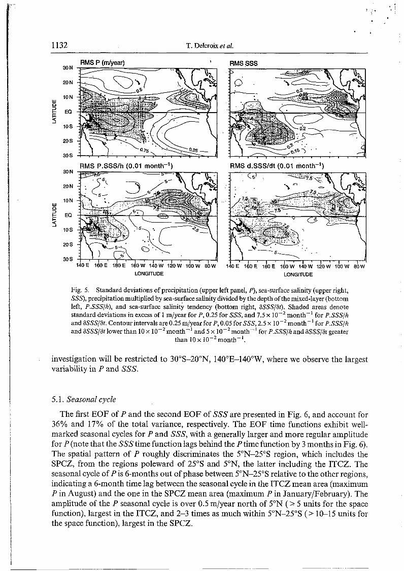
The patterns of standard deviation of P (op) and SSS (o3) are shown in Fig. 5. The standard deviations of estimated P are largest (op > 1 m/year) in regions of heavy rainfall associated with the ITCZ and the SPCZ, and in part of the warm pool. Maximum op values are located near the Solomon Islands in the southern hemisphere, and off Costa Rica in the northern hemisphere. The patterns of maximum standard deviations of the SSS data (o3 > 0.25) appear parallel to the ITCZ, with largest values in the east, and in the vicinity of the SPCZ. (Values north of 25"N near 150"W are not considered here). Using mean mixed- layer depths (Fig. 4), the standard deviations of P.SSS/h (op.slh) and aS/at (oas&) are also presented (Fig. 5) in order to compare the P and SSS changes in the same units (see equation (2a)). Maximum amplitudes (> 7.5 x low2 month-') in are located in the convergence zones and in the western Pacific warm pool, with similar values, except in the eastern part of the ITCZ where the SSS data distribution is very sparse (Fig. 1). As we will demonstrate in the following section, the correspondence between the patterns of P and SSS changes chiefly reflects the P and SSS relationships at seasonal and interannual timescales.

and

5. SPACE/TIME VARIABILITIES

Calculation of the EOFs of these data enables us to examine the spatially and temporally coherent variability of P and SSS. Given the time/space distribution of SSS data (Fig. I), continuous time-series cannot be derived over the whole basin. Hence our domain of

1132

i 1 1 : . ,

' . - 1

T. Delcroix et al.

I RMS P (wear) RMS SSS 30N

20 N

10N n t EQ

10 s

20 s

30 S

w 3

3

RMS P.SSS/h (0.01 month-') RMS d.SSS/dt (0.01 month-')

140E 160E 180E 16OW 14OW 120W 1oOW 80W

LONGITUDE LONGITUDE

Fig. 5. Standard deviations of precipitation (upper left panel, P), sea-surface salinity (upper right, SSS), precipitation multiplied by sea-surface salinity divided by the depth of the mixed-layer (bottom left, P.SSS/h), and sea-surface salinity tendency (bottom right, aSSS/at). Shaded areas denote standard deviations in excess of 1 m/year for P , 0.25 for SSS, and 7.5 x lo-* month-' for P.SSS/h and aSSS/at. Contour intervals are 0.25 mlyear for P, 0.05 for SSS, 2.5 x loF2 month-' for P.SSS/h and aSSS/dt lower than 10 x lo-* month-' and 5 x month-' for P.SSS/h and 8SSSlat greater

than 10 x month-'.

investigation will be restricted to 3O0S-20"N, 14O"E-14O0W, where we observe the largest variability in P and SSS.

5.1. Seasonal cycle

The first EOF of P and the second EOF of SSS are presented in Fig. 6, and account for 36% and 17% of the total variance, respectively. The EOF time functions exhibit well- marked seasonal cycles for P and SSS, with a generally larger and more regular amplitude for P (note that the SSS time function lags behind the P time function by 3 months in Fig. 6). The spatial pattern of P roughly discriminates the 5ON-25"S region, which includes the SPCZ, from the regions poleward of 25"s and 5"N, the latter including the ITCZ. The seasonal cycle of P is 6-months out of phase between 5ON-25"S relative to the other regions, indicating a 6-month time lag between the seasonal cycle in the ITCZ mean area (maximum P in August) and the one in the SPCZ mean area (maximum P in January/February). The amplitude of the P seasonal cycle is over 0.5 m/year north of 5"N ( > 5 units for the space function), largest in the ITCZ, and 2-3 times as much within 5ON-25"S (> 10-15 units for the space function), largest in the SPCZ.

d

f

. ' . .I


P: EOF#l (36%) . , 20 N -3

-2

-1 E EO

t O

1

20 s 2

3

10N

æ

4 10s

30 S

SSS: EOF #2 (17%) 20 N

10 N

EQ 3 t 3 10s

20 s

30 S 140 E 160 E 180 E 160 w l b

.I

O

-.l

W

74 76 78 I 80- 82 84 86 88

1 1 1 1 1 1 1 1 1 1 1 1 1 1

I I I I I I I I I I I ; ' I I D J F M A M J J A S O N D J

LONGITUDE

Fig. 6 . Spatial patterns of the first EOF of precipitation (upper left panel) and second EOF of sea- surface salinity (bottom left), together with the associated 1974-1989 time functions (upper right), and the 12 mean months constructed from the 1974-1989 time functions (bottom right). The scale of the precipitation time function is to the left, whilst the scale of sea-surface salinity is to the right and reversed. The sea surface salinity time function lags behind the precipitation time function by three months. In the lower-right panel, the error bars denote the mean monthly standard deviations. The product between the spatial pattern and the time function is the anomaly (departure from the mean),

in mlyear for precipitation.

The spatial pattern of SSS differentiates a northwest-southeast oriented band including the SPCZ, from the remaining areas, including part of the ITCZ (east of 170°W), the equatorial band and southern latitudes. There is a 6-month time lag between the northwest- southeast oriented band (maximum SSS in October) and the other regions (maximum SSS in March/April). The amplitude of the SSS seasonal cycle is over 0.05 for the northwest- southeast band ( > O. 1 unit for the space function) and 2-4 times less elsewhere (0.05 for the space function). The SSS spatial pattern reverses sign north and south of about 2"S, whereas the shift is at 5"N for the P spatial pattern, indicating that at seasonal timescales P and SSS changes are not related in the equatorial band. Interestingly, there is a hint of linear trends for SSS and P between the 1976 and 1982-1983 El Niño, as well as between the 1982-1983 and 1987 El Niño; the reason for this is unclear.

The seasonal SSS time function lags behind the seasonal P time function by 2-3 months (Fig. 6), as determined from time-lag correlation analysis. In Òther words, minimum (maximum) SSS occurs 2-3 months after maximum (minimum) P. If SSS changes are mainly governed by P changes, this lag may be understood mathematically from equation (5). In fact. for h constant. when P is sinusoidal with a 1-vear Deriod. Sis a auarter cvcle out

1134 T. Delcroix er d.

P; EOF #2 IZO%) 20 N .2

IQ N .i

EQ 3 t o 4 10s

-- 1 20 s

90s -.2 SSS: EOF#I {24%)

. . ._ . -3

-2

-1

o

1

2

W LONGITUUE

Fig. 7. Same as Fig. 6 for the second BOF of precipitation (upper left panel) and first EOF of sea- surface salinity (bottom left). The sea-surface salinity time function lags behind the precipitation time function by one month. The lower-right panel is the monthly values of the Southern Oscillation Index

smoothed with a 3-month Harming filter; note that the vertical axis is reversed.

1. This lag may be understood physically by of phase with P [P‘ = sin(ot) = > S- e noting that when the seasonal cycle of P is sinusoidal, with a 1-year period, the rainfall amount is above the annual mean, and so tends to lower SSS, for 3 months after its maximum value. Hence, the SSS seasonal cycle is consistent with the P seasonal cycle in regions where the spatial patterns in P and SSS are of the same sign, i.e. in the mean areas of the ITCZ and SPCZ. However, in these areas, the peaks of P patterns appear to be displaced to the northwest of the S peaks, indicating that the local effects of the P changes are in no way sufficient to explain the SSS changes at seasonal timescales. This large-scale result is in agreement with previous findings derived from alongtrack SSS data and sporadic P station measurements (e.g. Delcroix and Hbnin, 1989, 1991).

h cos(wt)

5.2. ENS0 anomalies

The second EOF on P and the first EOF on SSS are presented in Fig. 7 and account for 20% and 24% of the total variance, respectively. Time-lag correlation analysis between the P and SSS time functions indicates that P changes occur 1-2 months before SSS changes. (Note that the SSS time function lags behind the P by one month in Fig. 7.) The P and SSS time functions present a very good correspondence with the Southern Oscillation Index (SOI, Fig. 7), with peak values during the 1975 La Niña, the 1976-1977,1982-1983 and 1987 Los Niños, and the 1988-1989 La Niña. The best correlation between the P (SSS) time


function and the SOI is R = 0.58 (R = 0.74), obtained when the P (SSS) time function lags behind the SOI by 1-2 months (3-4 months). The product between the time functions and the spatial patterns measures the strength of the ENSO-related P and SSS changes, which exceed 1-2 m/year and 0.2-0.4, respectively.

The spatial patterns of the ENSO-related changes of SSS roughly discriminate the 1O"N- 10"s region (> O values) from the regions south of 10"s and north of 1O"N. Within about 1 0"N-loos, fresher-than-average (saltier-than-average) SSS appears during an El Niño (La Niña) event, with extreme SSSdecrease (increase) at about 2"S-170°E. East of 165"E, these SSS changes are consistent with increases (decreases) in rainfall, which occur in a broad band centred near 2"s latitude. South of about loos, saltier-than-average (fresher-than- average) SSS emerges during an El Niño (La Niña) event, with maximum SSS increases (decreases) near the Fiji islands (18"S-l78"E). These SSS changes can be related to El Niño- related rainfall shortage (La Niña-related enhanced precipitation) along an axis extending SE from Papua, New Guinea. North of about 10"N, P changes cannot explain SSS changes, probably due to the influence of E, which is greater than P (Fig. 3). These results are in qualitative agreement with the P analysis of Ropelewski and Halpert (1987) and the SSS analysis of Delcroix and Hénin (1 99 1). -

The coincidence between ENSQ-related P and SSS changes does not apply west of 165"E in the equatorial band, where the mean SSS exhibits positive eastward and poleward gradients (Fig. 3). There, during El Niño (La Niña), it is likely that advection of less (more) saline water by unusual eastward (westward) oceanic currents, in addition to possible effects of equatorward (poleward) Ekman salt advection associated with westerly (easterly) wind anomaly, downwelling (upwelling) processes or evaporation influence the SSS distribution. For example, with 0.6 unit of salinity change over 30" longitude (Fig. 3), a realistic zonal current anomaly U= 0.5 m/s would yield an advective term U& of 0.2 per month, which is consistent with Fig. 7. Right at 0-165"E, a concordant result was obtained by Sprintall and McPhaden (1994), who found that SSS changes were mostly influenced by upwelling and horizontal advection during the 1988-1989 La Niña and by freshwater fluxes during the 1989-199 1 ENSO-like condition. To a lesser extent, the effects of salt advection by oceanic currents might also be suspected south of about loos, in particular with a poleward (equatorward) displacement of the large-scale anticyclonic gyre center during El Niño (La Niña) and the accompanying modifications of the southern branch of the south equatorial current (Delcroix and Hinin, 1989). The contribution of advective processes to changes in the SSS is thus manifest, especially in the far western Pacific warm pool, but the degree of their influence cannot be rigorously established.

Summarising, during El Niño (La Niña), the prominent atmospheric circulation changes consist of an eastward (westward) shift of the ascending branch of the Walker and Hadley cells, as observed by previous investigators (e.g. Lau and Chan, 1983). This shift implies unusually high (low) rainfall and fresher-than-average (saltier-than-average) SSS over the western-central equatorial Pacific, together with compensating low (high) rainfall and thus saltier-than-average (fresher-than-average) SSS south of about 10"s latitude.

5.3. Correlation

The observed agreement in phase and location between P and SSS seen in Figs 6 and 7 does not tell us whether the P changes are large enough to explain the observed SSS changes. To help answer this question, the seasonal and interannual ENSO-related

1136

-

T. Delcroix et al.

10 N

W n EQ 3 Ir 4 10s

20 s

30 S 140 E 160 E I80 E 160 w 140 w

LONGITUDE

Fig. 8. Correlation coefficients (R) between the 1974 and 1989 monthly precipitation time series and sea-surface salinity time series lagging by 2 months, both reconstructed from the first 2 EOF

presented in Figs 6 and 7. Shaded area denotes R < -0.4.

components of the P and SSS fields were reconstructed from the first two EOFs. The correlation of the reconstructed fields, when SSS changes lag behind the P changes by 2 months, is shown in Fig. 8. Only absolute value contours exceeding the approximate 95% confidence interval O(0.4) are plotted. As expected from the EOF analysis, the P and SSS changes are inversely related (R< -0.4) in a broad zone between about 10"N and 10"s east of 170"E and in the SPCZ and ITCZ areas. Also notable in Fig. 8 is the positive correlation in the far western equatorial Pacific, which indicates that the local SSS changes must result from evaporation, advection or mixing processes rather than from local P changes.

To investigate whether the magnitude of the P changes can account for the magnitude of the SSS changes, we present (Fig. 9) the ensemble relation between S-'S, and P (see equation (5)) in the region where the phases between SSS and P changes are inversely related (R< -0.4 in Fig. 8). The values of P were produced by considering all the values that fall within each Y'S, bin of 4 x lop3 year-' for all months. The numbers of S-'S, values in each bin ( N in Fig. 9) are normally distributed, indicating, as expected, that the probabilities of positive and negative SSS changes over the full record length are equal. The intercept of P versus S-'S, is almost zero, indicating that the terms related to mean salt advection, mean precipitation and evaporation balance each other (see equation (4)). Of most interest, the slope of P versus S-IS, provides an indirect estimate of the mean thickness, h, of the mixed layer (equation (5)), and has a value of 3 1 m. For comparison, we computed a mixed-layer depth of h=45 f 15 m (the second number is one standard deviation) from the mixed-layer depth in Fig. 4 sampled in the R < - 0.4 region of Fig. 8. Also, Lukas and Lindström (1991) found h = 29 f 24 m in the western equatorial Pacific (143"E-l55"E), and Delcroix et al. (1992) found h = 36 +26 m within 5"S-l5"S along 165"E (where R < -0.4). The agreement of our indirect estimate of h (=31 m) with direct measurements (45 f 15,29 + 24, and 36 _+ 26 m) implies that, in the mean, the simplification in equation (5) applies reasonably well to our measurements. In regions where R < - 0.4 in


h

O O O

x 7

U

âi E Q

2

Fig. 9. (S- * as/%) bins. Also shown are the population (N, broken line) of the bins. Both P' and N are for the region

where R < -0.4 in Fig. 8.

Bin-averaged precipitation anomaly (I", m/year; full line) as a function of (S-' &Slat) for 4 x

Fig. 8, the magnitude of seasonal and interannual SSS changes is thus globally consistent with the magnitude of P changes. However, the standard deviation of the P anomaly within each S-'S, bin (not shown in Fig. 9) ranges from 0.5-1.1 m/year, which emphasises the inadequacy of the global relation for a specific time or location.

6. DISCUSSION

As noted in the Introduction, one aspect of the present work is to complement previous studies, which have neither examined the large-scale relation between P and SSS nor attempted to use observed SSS changes to infer P changes, or vice versa. Given the findings discussed above, the question remains whether the relations we documented between large- scale SSS and OLR-derived P can be used in statistical models to permit us to estimate P changes using known SSS changes or to forecast SSS changes from observed (estimated) P.

As a first step in answering this question, we restricted our attention to the seasonal and interannual ENSO-related changes, as illustrated by the EOF analysis, and we assumed that the P-SSS relationships are linear, so that P or SSS changes may be derived by a simple linear regression (LR) model. As far as the LR model is concerned, deriving P from SSS or SSS from P is similar, and only P estimates derived from known SSS are presented here. The P and SSS fields were reconstructed from the first and second EOF, as in Section 5.3, and a cross-validation technique (Mosteller and Tukey, 1977) was employed to specify P during months not used in the LR model. In this technique, the 192 months of P (dependent) and SSS (independent) data were divided into 16 segments, each of 12-month duration. The LR model was run using the data of 15 segments in P and 15 segments in SSS shifted in time by various lags. The model was then used to specify P in the remaining segment using the SSS data of the corresponding segment. This process was successively repeated by changing the excluded segment, which yields 192 independent specifications of hindcast P which may be compared to the observed values. Using segments ranging from 6 to 36 months in duration did not affect our conclusion.

1138 T. Delcroix er al.

Correlation Coeff., Observed versus Hindcastp RMS diff., Obsewed minus Hindcast P (Wear) 20 N

1ON

EQ 3 t 5 10s

20 s

30 S 140 E 160 E 180 E 160 W 140 W ow

LONGITUDE LONGITUDE

Fig. 10. Correlation coefficient (left panel) and rms difference (right panel) between observed and hindcast precipitation anomalies (see the text for details). Shaded areas denote R > 0.4 (left panel)

and the rms differences > 0.75 mlyear.

The correlation coefficients and the rms differences between the hindcast and observed P are shown in Fig. 10. As might be expected from Fig. 8, the best hindcast specifications (R = 0.4- 0.7), obtained when SSS lags behind P by 2 months, are located in the SPCZ, and in the ITCZ and the equatorial region east of the dateline. In these regions the rms differences range between 0.5 and 1 m/year, i.e. 80% of the rms of the OLR-derived seasonal and interannual P signals (not shown here but with similar patterns as in Fig. 5). Hence, the simple LR model offers potential skill for hindcasting the timing of seasonal and ENSO- related P changes, but it does exhibit poor skill in predicting the magnitude of P changes.

Several important weaknesses of the LR model are evident. We neglect entirely the contribution of evaporation and salt advection as well as changes in the mixed-layer depth in modulating SSS (terms E, A and h in equation(2)). The possible contribution of these three factors is tentatively presented below. First, to get a rough idea of the effect of evaporation (E> in the absence of E time-series, Fig. 1 1 presents the mean (V) and standard deviation (o,) of the wind speed computed over the 1974-1989 period (note that Fig. 11 is presented over the whole basin, for consistency with the first figures). Based on the commonly used bulk formulae, E can be written as:

E = PuLCeV(qs - qu) (6) where pa is the air density (1.225 kg/m3), Ce is the Dalton number (15 x lop4), (qs-qn) is the sea-air humidity difference and the other terms are as defined previously. Assuming for the sake of this discussion that (qs-qa) is constant and equal to 6g/kg (see Esbensen and Kushnir, 1981; their Fig. 1.78), the standard deviation of E (oE) due only to the wind speed changes represented by o, would be greater than 0.5 m/year in regions where o, > 1.5 m/s, i.e. essentially in the convergence zones and in part of the warm pool. Given the standard deviation of P in these regions (Fig. 5), this simple test suggests that the amplitude of E changes (oE) are 30-50% of those of P changes (op), stressing the likely role of E in modifying SSS. Secondly, meridional and zonal salt transports also induce SSS changes not linked to P changes. The SSS changes linked to the meridional Ekman salt transport associated with the trade winds was noted in Section 4; as a sensitivity study, those linked to the varying zonal salt transport are now estimated in the North Equatorial Countercurrent

Precipitation and sea-surface salinity in the tropical Pacific Ocean 1139 f

J

W

3 o

30 N

20 N

10N

EQ

10s

20 s

30 S

Mean Wind SDeed (d.9 . .

5:' 3

l'l'l'l'i

LONGITUDE 140E 160E 180E 160W 14OW 12OW IOOW 8OW

RMS Wind Speed (ds)

I b E 16OE 1 b E l b W 1 b W l2OW 1 b W 8OV

LONGITUDE

Fig. 1 1. Mean (left panel) and standard deviation (right panel) of the wind speed during the 1974- 1989 period. Shaded areas denote wind speed and standard deviation in excess of 6 and 1.5 mis,

respectively. Contour intervals are 1 m/s (left panel) and 0.25 m/s (right panel).

(NECC) region which is also the ITCZ region. In the central Pacific (152"W), based on Reverdin et al. (1994); their Fig. lo), the seasonal changes of the NECC can be reasonably written as a sine function of the form:

u = u0 + a sin[o(t - 711 (7)

where u. = 25 cm/s, a = 15 cm/s, o = 2x112, and t is the month number. If the zonal gradient of salinity (SJ is constant, of the order of 0.2 per 20" longitude as in Fig. 3, then the standard deviation of zonal salt advection linked to the NECC seasonal changes (u S,) would be equal to 2.5 x lod2 month-', i.e. about 25% of the standard deviation of the SSS tendency (St; Fig. 5). At seasonal timescales, the effect of salt advection in the NECC region is thus not negligible in changing SSS; a similar conclusion would hold at interannual timescale (see Meyers and Donguy, 1984). Thirdly, the mixed-layer depth exibits not only spatial variations (Fig. 4) but also temporal variations at both seasonal (Sprintall and Tomczak, 1990) and interannual (Sprintall and McPhaden, 1994) timescales. As noted in Section 5, such variations can be very strong in the warm pool, fundamentally altering the assumption that P and SSS are linearly related. Hence, while the simple LR model is limited, it has the advantage of isolating the locations of consistent P and SSS changes at seasonal and interannual timescales.

To summarise and conclude, the present study has explored the links between means and variations in the tropical Pacific sea-surface salinity and OLR-derived precipitation during the 1974-1989 period. EOF analysis has revealed that the dominant SSS-P changes span large spatial scales, and that the most significant SSS-P relationships are in the ITCZ east of the dateline, in the SPCZ, and in the central-western equatorial Pacific, at seasonal and ENSO timescales. The inferences derived from this analysis were used in designing a simple linear regression model to attempt to specify P changes based upon a knowledge of SSS changes. This model provides moderate hindcast skill in some regions. In the SPCZ, and between 180 and 150"W in the equatorial region and the ITCZ, SSS changes could be used to infer the timing, but not the magnitude, of P changes. Taken alone, sea-surface salinity is thus a mediocre indicator for quantifying precipitation changes at seasonal and ENSO timescales. Nevertheless, we wish to emphasise that this study is only one step toward

1140 T. Delcroix e t al.

improving our knowledge of P changes with the aid of oceanic variables (unique in the present case). It is clearly desirable to combine statistical models with dynamical models, and to use additional observed, estimated or modeled oceanic and atmospheric variables (such as mixed-layer depth, current, and evaporation) for improving estimates of open- ocean precipitation. . .

Acknowledgements-The present SSS data set represents the combined efforts of many ORSTOM scientists involved in the surface ship-of-opportunity program, and in particular owes much to Jean-René Donguy. Additional SSS data derived from hydrocast and CTD measurements were provided by Alain Dessier. The wind, world ocean and evaporation data sets were obtained from J. J. O’Brien, S. Levitus and Y . Kushnir, respectively. Fruitful discussions and comments from Pierre Rua1 and Mansour Ioualalen, together with the suggestions of two anonymous reviewers, were helpfulin improving the manuscript. For one of the authors (V.P.), some aspects of this work represent a “Stage d’Approfondissement de 1’Ecole Nationale de la Météorologie de Toulouse-Mirail”, performed while visiting the ORSTOM Center in Noumea. All these contributions are gratefully acknowledged.

REFERENCES

Arkin P. A. (1984) An examination of the Southem Oscillation in the upper tropospheric tropical and subtropical wind field. Ph.D. dissertation, University of Maryland, 240 pp.

Arkin P. A. and B. N. Meisner (1987) The relationship between large-scale convective rainfall and cold cloud over the Western Hemisphere during 1982-1 984. Monthly Weather Review, 115, 51-74.

Arkin P. A. and P. E. Ardanuy (1989) Estimating climatic-scale precipitation from space: a review. Journal of Climate, 2, 1229-1238.

Delcroix T. and C. Hénin (1989) Mechanisms of subsurface thermal structure and sea-surface thermohaline variabilities in the southwestem tropical Pacific during 1979-1985. Journal of Marine Research, 47,777-8 12.

Delcroix T. and C. Hénin (1991) Seasonal and interannual variations of sea-surface salinity in the tropical Pacific Ocean. Journal of Geophysical Research, 96, 22,135-22,150.

Delcroix T., G. Eldin, M. H. Radenac, J. Toole and E. Firing (1992) Variation of the western equatorial Pacific Ocean, 1986-1 988. Journal of Geophysical Research, 97, 5423-5445.

Donguy J.-R. (1 987) Recent advances in the knowledge of the climatic variations in the tropical Pacific. Progress in Oceanography, 19, 49-85.

Donguy J.-R. and C. Hénin (1975) Surface waters in the north of the Coral Sea. Australian Journal of Marine and Freshwater Research, 26, 293-296.

Donguy J.-R. and C. Hénin (1976) Relations entre les précipitations et la salinité de surface dans l’océan Pacifique tropical sud-ouest basées sur un échantillonnage de surface de 1956 H 1973. Annales Hydrographiques, 4,53- 59.

Donguy J.-R. and C. Hénin (1977) Navifacial conditions in the northwest Pacific Ocean. Journal of the Oceanographic Society of Japan, 33, 183-189.

Dorman C. E. and R. H. Bourke (1979) Precipitation over the Pacific Ocean, 30°S-60”N. Monthly Weather Review, 107, 896-910.

Esbensen S. K. and Y . Kushnir (1981). The heat budget of the global ocean: an atlas based on estimates from surface marine observations. Climate Research Institute, report no. 29, Oregon State University, Corvalis, OR 97331, U.S.A.

Hires R. and R. Montgomery (1972) Navifacial temperature and salinity along a track from Samoa to Hawaii, 1975-1965. Journal of Marine Research, 30, 177-200.

Goldenberg S. and J. O’Brien (1981) Time and space variability of tropical wind stress. Monthly Wearher Review, 109, 1190-1207.

Jaeger L. (1976) Monatskarten des Niederschlags für die ganze Erde. Berichte des Deutschen Wetterdienstes, No. 139 (Band 18). Offenbach A. M., 33 pp.

Janowiak J. E. (1992) Tropical rainfall: A comparison of satellite-derived rainfall estimates with model precipitation forecasts, climatologies, and observations. Monthly Weather Review, 120, 448462.

Janowiak J. E. and P. A. Arkin (1990) Rainfall variations in the tropics during 1986-1989. Journal of Geophysical Research, 96(supplement), 3359-3373.

Janowiak J. E., P. A. Arkin, P. Xie, M. L. Morrissey and D. R. Legates (1995). Rainfall variability in the tropical Pacific inferred from several independent data sources. Journal of Climate, 8, 28 10-2823.


Lau K. M. and P. H. Chan (1983) Short-term climate variability and atmospheric teleconnections from satellite- observed outgoing longwave radiation. I: Simultaneous relationships. Journal of Atmospheric Sciences, 40, 2735-2750.

Levitus S. (1982) Climatological atlas of the world ocean, NoAA Prof. Pap., 13, 173 pp., US Govt. Print. OMice, Washington, DC, 1982.

Levitus S. (1986) Annual cycle of salinity and salt storage in the world ocean. Journal of Physical Oceanography,

Liu W. T. (1988) Moisture and latent heat flux variabilities in the tropical Pacific derived from satellite data. Journal of Geophysical Research, 93, 6749-6760.

Lukas R. (1990) The role of salinity in the dynamics and thermodynamics of the western Paci@ warm pool. Proceedings of the International TOGA scientific conference, 16-20 July 1990, Honolulu, Hawaii, pp. 73- 82.

Lukas R. and E. Lindström (1991) The mixed layer of the western equatorial Pacific Ocean. Journal of Geophysical Research, 96, 3343-3358.

Meyers G. and J.-R. Donguy (1984) The north equatorial countercurrent and heat storage in the western Pacific odan during 1982-1983. Nature, 312, 258-260.

Miller J. (1976) The salinity effect in a mixed layer ocean model. Journal of Physical Oceanography, 6, 29-35.

_ -

16, 322-343.

i Morrissey M. L. (1986) A statistical analysis of the relationships among rainfall, outgoing longwave radiation and I E the moisture budget during January-March 1979. Monthly Weather Review, 114, 93 1-942.

Morrissey M. L. and J. S. Greene (1993) Comparison of two satellite-based rainfall algorithms using Pacific atoll

Mosteller T. and J. Tukey (1977) Data analysis and regression. Addison Wesley, 586 pp. Motel1 C. E. and B. C. Weare (1987) Estimating tropical Pacific rainfall using digital satellite data. Journal

Reid J. L. (1969) Sea surface temperature, salinity and density of the Pacific Ocean in summer and in winter.

Reverdin G., C. Frankignoul, E. Kestenare and M. McPhaden (1994) Seasonal variability in the surface currents

Ropelewski C. F. and M. S. Halpert (1987) Global and regional scale precipitation patterns associated with the El

Spencer R. W. (1993) Global oceanic precipitation from the MSU during 1979-1991 and comparison to other

Sprintall J. and M. Tomczak (1990) Salinity considerations in the oceanic surface mixed layer. Ocean Sciences

Sprintall J. and M. Tomczak (1992) Evidence of the barrier layer in the surface layer of the tropics. Journal of

, Sprintall J. and M. J. McPhaden (1994) Surface layer variations observed in multiyear time-series measurements

Sui C . H., K. M. Lau and A. K. Betts (1991) An equilibrium model for the coupled ocean-atmosphere boundary

Taylor R. C . (1973) An atlas of Pacific Islands rainfall. Department of Meteorology Publication No. 25, The

Weare B., P. T. Strub and M. D. Samuel (1981) Annual mean surface heat fluxes in the tropical Pacific Ocean.

Xie P. and P. A. Arkin (1995) An intercomparison of gauge observations and satellite estimates of monthly

Yo0 J.-M. and J. M. Carton (1988) Outgoing longwave radiation derived rainfall in the tropical Atlantic, with

raingage data. Journal of Applied Meteorology, 32, 41 1-425.

Climate Applied Meteorology, 26, 1436-1446.

Deep-sea Research, 16 (Suppl.), 21 5-224.

of the equatorial Pacific. Journal of Geophysical Research, 99, 20,323-20,344.

Niíio/Southern Oscillation. Monthly Weather Review, 115, 1606-1626.

climatologies. Journal of Climate, 6, 1301-1326.

Institute, Rep. 36, University of Sydney, 170 pp.

Geophysical Research, 97, 7305-73 16.

from the western equatorial Pacific. Journal of Geophysical Research, 99, 963-979.

layer in the tropics. Journal of Geophysical Research, 96, 3 15 1-3 164.

University of Hawaii, Honolulu, HI 96822.

Journal of Physical Oceanography, 11, 705-717.

precipitation. Journal of Applied Meteorology, 34, 1143-1 160.

emphasis on 1983-1984. Journal of Climate, 1, 1047-1054.

. . ,

i

precipitation and sea-surface salinity in the tropical...

Documents