PRAKLA-SEISMOS INFORMATION No.46

Streamer Positioning and Coverage Control /\

PRAKlA·SEISMDS

V V

Introduction

Advanced 3-D marine surveys nowadays require a much higher degree of accuracy in streamer positioning than was possible until recently. Dense grids in conjunction with multi-line and strike line shooting make the tolerances allowable for the determination of streamer positions even more stringent.

In order to obtain all angles and distances with the required accuracy PRAKLA-SEISMOS has added new features to the existing measuring systems and the associated com­puter software. These efforts aim to pinpoint each com­mon reflection point to within ± 10 m. The new tech­niques to resolve the difficulties involved were adopted after careful research into the problems of sensing angles and tensions, pertaining to the seismic streamer, as primary input parameters in deriving the streamer position.

Streamer Tracking System

General The following hardware/ software components are utilized in deriving streamer locations under the new scheme:

• Gyro Compass System: to reduce the error against true North to within ± 0.12 degree.

• Two Independent Streamer Tracking Systems

1. Magnetic Heading Compasses: arrayed along the streamer to record the subsurface direction of the streamer sections.

2. Bearing Reference

2.1: Precision Direction Finding System to determine the tail end of the streamer to with in ± 0.2 degree.

2.2: Manual Direction Finders to determine the residual installation errors of the gyro system and to calibrate and check the Precision Direction Finding System.

Fig. 1: Presentation of Hardware Components

Gyro Compass System

Cable Departure Angle Measuring Unit

The Precision Direction Finding System, developed by PRAKLA-SEISMOS, controls and adjusts the streamer compasses. Ref­eren ce North is provided by a specially assembled multiple gyro system. An au­tomated control system monitors all on­board events in realtime.

In the post-processing stage, a highly reliable motion model is established by cross-correlating multiple se­quences of angle measurements, thereby taking full ad­vantage of the redundancy in the data. This procedure improves the realtime data significantly.

• Cable Departure Angle Measuring Unit: to record the horizontal angle between the vessel 's axis and the towing cable of the streamer to within ± 0.2 degree.

• Stretch Section Length Measuring Unit: to record the actual distance between the towing cable and the first hydrophone group to within ± 1.0 metre.

• Realtime Processing and Quality Cont rol: to pro­vide a quick reference of headings, positions and coverage on monitors, hardcopies and plotter.

/ Magnelie Heading compass~s ____

Stretch-Section Length Measuring Unit

Precision Direction Finding System with Optical Bearing Control System

2

Streamer Tracking System

Description 01 Components:

Gyro Compass System

The gyro system is the master instrument which provides the reference North for all bearing measurements con­ducted from the survey vessel. The optimization of the ref­erence North is achived by integrating a multiple set of gyro

compasses specially designed and manufactured for PRAKLA-SEISMOS by C. PLATH. A microprocessor checks the plausibility of the individual gyro readings and computes an improved true North to within ± 0.12 degree.

Fig. 2: Improved Reference North

REFERENCE NORTH = ± 0.12°

MICROPROCESSOR

C. PLATH NAVIGAT 11 Gyro system ~--------------------~

3

Streamer Tracking System

Two Independent Streamer Tracking Systems:

1. Magnetic Heading Compasses: the relative positions of the streamer are derived from the angle indications of miniature magnetic compasses arrayed along the streamer at set intervals. The compasses used are manufactured by SYNTRON.

Fig. 3: Streamer with Heading Sensors

Gyro North = true North (Nt)

Position of the Hydrophone Groups

Magnetic North (Nm)

2. Bearing Reference

2.1. Precision Direction Finding System (PDF) The PRAKLA-SEISMOS Precision Direction Finder which operates in the VHF band compares the phase angle of a continuous wave (CW) transmitted from the tailbuoy. The PDF provides the angle between true North and the tail end of the streamer continuously. The system is accurate to within ± 0.2 degree.

4

Reception of CW and Equal Phase Balancing of

Twin Antenna Beam

Angle between Antenna Beam and Ship's Axis

---

\I

-----.c ____ 1: -_ 0 ____ z

e >.

"

Tailbuoy Position

Deviation: Individual Magnetic Compass Error

Sailed Track

Fig. 4: Precision Direction Finding System

Transmission of Continuous Wave ( CW )

\ I

Tailbuoy Position

Sailed Track

Fig. 5: Manual Direction Finders

Optical Direction Finders

jeu rre n1

Streamer Tracking System

2.2. Manual Direction Finders Three Manual Direction Finders serve as the function control for the PDF. They are installed such that un­interrupted sighting of the tailbuoy may be maintained at all.times. A push-button release mechanism permits instantaneous freezing of the tailbuoy bearing with respect to the ship's axis. The navigation computer derives the north orientation automatically by adding the ship's heading to this measurement. The statistical average of a set of observations, computed in realtime , provides the adjusted bearings for calibration and control of the PDF.

Tailbuoy

==--=­=---=--=--

Sailed Track

5

Streamer Tracking System

Cable Departure Angle Measuring Unit

The deflection angle between the ship's axis and the towing cable is continuously recorded to determine the shipl streamer lateraloffset. The device consists of universal joints, flexible shafts and synchro units. Angles are recorded to within ± 0.2 degree.

Fig. 6: Cable Departure Angle Measuring Unit

Simplified mechanism--

Induction synchro unit

Stretch Section Length Measuring Unit

Variations in streamer stretch section length are sensed by asounding system developed by HONEYWELL ELAC. It records the required data to within ± 1.0 m.

Fig. 7: Stretch Section Length Measuring Unit

Varying distance

Departure angle

Live sections Recei er

6

Streamer Tracking System

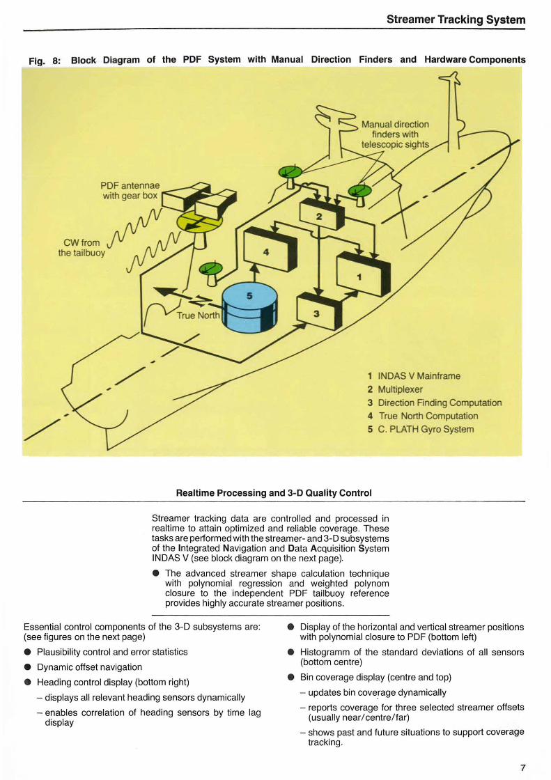
Fig. 8: Block Diagram of the PDF System with Manual Direction Finders and Hardware Components

CWfrom the tailbuoy

Manual direction finders with

tetescopic sights

1 INDAS V Mainframe

2 Multiplexer

3 Direction Rnding Computation

4 True North Computation

5 C. PLATH Gyro System

Realtime Processing and 3-D Quallty Control

Streamer tracking data are contralted and pracessed in realtime to attain optimized and reliable coverage. These tasks are performed with the streamer- and 3-D subsystems of the Integrated Navigation and Data Acquisition System INDAS V (see block diagram on the next page).

• The advanced streamer shape calculation technique with polynomial regression and weighted polynom closure to the independent PDF tailbuoy reference pravides highly accurate streamer positions.

Essential contral components of the 3-D subsystems are: (see figures on the next page)

• Display of the horizontal and vertical streamer positions with polynomial closure to PDF (bottorn left)

• Plausibility control and error statistics

• Dynamic offset navigation

• Heading contral display (bottom right)

- displays alt relevant heading sensors dynamicalty

- enables correlation of heading sensors by time lag display

• Histogramm of the standard deviations of alt sensors (bottom centre)

• Bin coverage display (centre and top)

- updates bin cove!age dynamicalty

- reports coverage for three selected streamer offsets (usualty near/ centre/far)

- shows past and future situations to support coverage tracking.

7

Streamer Tracking System

Fig. 9: Realtime Processing and 3-D Quallty Control Block Diagram

Bin Coverage Display

Bin Coverage Hardcopies Current FiII-ln Current Overfill

Streamer Offset­Presentation tor Screen and Hardcopy

Single Production Line

;I .. ir !r !

8

00 Subs

,..-._ .-i RadIo Na" • GraY! I Magne . e L-._ ._

--Live

3-D Qua/ity Control

Subsystem

I Operator Display

INDAS V MAJNFRAME

Streamer Tracking System

Bridge I Display I ....

@i!) Data

Storage

>­lU­_CI) 0.> ct}CI) 5-1

CJ) c Uj­ct}CI) CI) > (JCI) 0..J ...

Cl,

... o (1) (1) CI) (J-o CI) ... >

Cl, CI) -::J 0. C

...

..J

0-(1) CI) c> CI) CI)

C/)..J

9

Calibration

General

Recent experiences have proven that the newly de­signed streamer positioning and quality control sub­systems are perfectly suitable to determine and super­vise the calibration values 01 the gyro master re1erence, 01 the different bearings and 01 the magnetic compass headings.

Description of Calibration Procedures:

In order to maintain systems' functioning , high precision performance and self test capabilities at all times during a survey an extensive pre-mission calibration sequence is employed:

• Stationary calibrations of the multigyro system and manual direction finders using geodetic targets

• Calibration of the PDF system under operational survey conditions using the pre-calibrated manual direction finders

• Performance check of the magnetic compasses and determination of their instrumental and mounting fixed errors by calibration against the PDF reference.

Stationary Check 01 the "North Re1erence"

A port with suitable remote targets is required for this very important pre survey check procedure. After fixing the geodetic coordinates of the onboard optical direction finders these are aimed at remote targets. The computed minus

observed azimuths provide reliable correction figures for the residual installation errors. The cable departure angle measuring unit is checked at the same time.

Fig. 10: Check of the Residual Installation Errors of Master Gyro and Optical Direction Finders

10

Optional:

• Dynamic gyro test by cruising past a fix point under survey conditions, thereby continuously taking bearings using the manual direction finders.

• Overall system check by comparing computed with observed tail end positions using a second boat.

Calibration

In contrast to commonly used systems even varying calibration values are derived from the unique configu­ration and performance of the system:

• Geomagnetic daily and long term variations are indicated

• Sporadic jumps and instrumental variations of the magnetic compasses are revealed

Dynamic Check of the "North Reference"

The accuracy of the PDF System in a dynamic situation is dependent on the stability of the gyro compass system. The main source of errors is the oscillating characteristic of the gyros after significant ship maneuvers such as course changes or full turns. By cruising with the survey vessel

past fixed targets it has been proven that the gyro system remains stable even after ship's turns (see fig. 11). The second peak of the "Schuler period" (84.4 minutes) is reduced to ± 0.1 degree. This allows run-in distances to be significantly reduced.

Fig. 11: Check of the Oscillating Characteristic of the Master Gyro Compass System

~West East~

2°

10 min 10 min

1 hour 1 hour

2° 1+------- Schuler Period -------~

---- Ship's course controlled by means of a highly accurate positioning system

....-7F!:I!!!!!!!!!!!"'"--~_ Gyro compass' offset derived from computed minus observed azimuths

Computed azimuths using target and ship's position

- --- Observed optical bearings based on gyro master reference

Calibration

Calibration of the PDF

The. PDF is the master reference for streamer positioning. Therefore. careful calibration is performed as folIows:

Whilst sailing slowly on a zig zaging course. a1ternating by + / - 30 degrees. the observers aim at the tailbuoy and take bearings frequently with the manual direction finders. The electronically logged optical bearings are compared with the PDF bearings. displayed on a monitor and plotted as computed minus observed values on a graph as shown below.

Fig. 12: Ca libration of the PDF System

Tailbuoy transmitting CW

Fig. 13: Scatterplot of the PDF Calibration

z.o c !;j

" '" ;0 1.0 1.0

'" Z N

PDF-TESTS

PDF antenna

ON JUNE 9 . • 198'1

t . B

. . + . +~ .~ ~.~ ~ .~" .. . _~.;.,t. :.:.~-~ . . 1,1; • ~ __ ~ "".L~.\. B.0

.,;. , ;"''fJ.. ~ ,J... .. ~ .~ r .... -" ' ./. ' i + -_. .... r- ..... - ...-tI' • '-:' r:t t+-... +-: "~,. .. .., ~,.~-= .. --~::.~ .... .:-: .. ~. -:r t:':e

" ' ... . .. . ... !" . . .' . .. .., .....

" W -1.0 - 1.0 -t.a I

" '" -z.O

N ...... .. :: ~ " " ...... ~ öD ~ ..

CJ1 .. .. .. CXI .. co

0 0 0 0

12

<~ .'" ~~'Q ==' .. ~~ /-

N ~ . I\:) ....

0 0

Calibration

Calibration of the Streamer Heading Sensors

Stationary Calibration: Before using the magnetic com­passes in the streamer each sensor is calibrated in a labo­ratory which is completely compensated for any magnetic variations. Thereafter an individual deviation table, in steps of 15 degrees, is established for each sensor and fed into the navigation computer.

Fig. 14: Stationary Heading Sensor Deviation Func­tion The individual deviations of two streamer head­ing sensors are depicted as function graphs for two typical sensors.

Dynamic Calibration: During the seismic survey the indivi­dual deviation tables of the heading sensors are updated based on statistical evalutions. The updates are established by comparison of the heading sensors with each other and with the PDF in time-lag mode. Based on the updated sensor deviation corrections the streamer shape determination process, as part of the PRAKLA-SEISMOS Realtime Processing System, com­putes an adjusted streamer polynomial , which matches the PDF reference bearing to within ± 10 m at the tailbuoy.

10 _ Streamer compass No. 5201

0 0 ~TI~

-l:llllll ~ ~ - 2 -

0° 90° 180° 270° 360 0

Streamer compass No. 5189 1° -

0° ..-r::t T T T T ! r -,-... • , , . ----.. _ 10kLOJ I I p:===-- ~

Final Overall System Check (Optional)

To prove correct functioning of the streamer tracking system and the streamer shape as calculated by the realtime pro­cessing system the following check can be performed at the clients 's request:

A second vessel , equipped with an independent positioning system, sails very closely behind the tailbuoy, logs its own

position and measures the distance to the tailbuoy. The derived tailbuoy coordinates are compared with the respec­live coordinates computed by the realtime processing system. Instead of a second ship it is possible to use a fixed laser to measure the coordinates.

Fig. 15: Sketch of the Final Overall System Check

I Fixed platform

~~~~ce~r-r-(~~--------~-------------r------------~c-o-o-r-d-in-a-te-G--ri-d-+--~ ~eO ~ v~

~'i:>'U . ~\}~ 2' ~ e~~e O~~:?" ~

\..~s ~~ ,~-:>. (Q~ 0- iS"~

~~o­~ %% Vessel with ----1f-""......".---------+----~~ ~

independent "C>(Q

positioning system

Ship's track

Submerged streamer

affected by turbolent currents ~-..I. ___ S_eismiC survey "Fel

13

Post-Processing

General

Post-mission processing is to enhance the realtime streamer positions and to determine the locations of all streamer segments in the geodetic grid and thus to derive the most accurate subsurface positions. The processed data is stored on a positioning data file for use in further seismic processing. Various graphie representations are plotted at suitable seal es for control purposes and to support the seismic processing.

The raw information from all sensors is reprocessed using an integrated, advanced processing technique in order to observe a positioning accuracy to within ± 5 metres for subsurface locations in any given streamer environment.

Built in streamer compasses are strongly influenced by varying torsion and tension forces. Experience shows that their calibration state changes with variations in the local

environment. Therefore, one major task in post-processing is to redefine the pre-mission calibration values on a continuous basis, and not to consider them invarjant over the whole survey.

Special correlation techniques in conjunction with the independent PRAKLA-SEISMOS PDF system result in linewise caHbration functions for the streamer heading sensor system.

The outstanding accuracy of the PDF system becomes evident from the correlation between magnetic variations as recorded by a ground station and PDF functions (see part B in figure 17b).

Processing

The 3-D positioning sequence consists of 4 main phases (see flow diagram):

Phase 1 Phase 3

• Sensor data preparation • Determination of the streamer shape

Phase 2 • Weighted closure to tailbuoy

• Positioning of ship based locations Phase 4

• Processing of sensor data • Positioning of common reflection points

• Graphics representation

Streamer Positioning Sequence

Input Output

Non-seismic Field Data

.-- -11 I Formal Review Control Display

.- II I Inleractive Terminal "" . Editing . Profile Plots

I .. Data Organisation I • I I Ship Positioning .1 Shotpoint Location Map • I I

I Catibration I and Filtering Final Sensor Display

• 11

I \ Streamer Polygon I l Parameters tor Areal Graphics

I I Tailbuoy Adjustment Streamer Location Map IL

1 11 I CDP Posilioning Subsurface Scat1ergram

~ I • J Bin Orientalion I J I Bin Parameters Bin Graphics "I and Coverage \

I "\

• I 3-D Data Collection .. 3-D Data Tape j'L ~5

I Selsmic Processing

14

I ~: I

I

J

J

I

I I

I

Editing of gaps, spikes and sensor malfunctions along with a formal review of all input data are the main tasks during Phase 1. Plots and displays as Shown in fig. 17 c assist editing.

Phase 2 splits into ship positioning and 3-D sensor data processing. Ship positioning results in highly accurate geodetic positions for anten na and source (see fig . 16a).

3-D sensor data processing is performed in an "instanta­neous position domain", by removing the time-lag of the individual heading functions. They are now referenced to positions rather than times. This processing stage com­prises correlation, fine editing, filtering and calibration. The compasses are calibrated relative to each other for the time being. Individual correclions are derived and updated block­wise for continuous survey periods. The fixed deviation of the local magnetic field was reduced beforehand. In a second step the whole system is calibrated against the PDF reference (see figs. 17a und 17b).

In the instantaneous position domain additional reference headings can be interpolated between the observed com­pass functions to improve the integration of the streamer shape function (see fig . 18a).

Fig.16a: Location Map Based on Antenna Positions

Fig.16b: Location Map Based on Reference Reflection Points

Post-Processing

Final sensor displays as shown in figure 17c are produced in the r€incorporated time domain after completion of the phase 2 processing stage.

Cable departure angles, streamer headings and stretch section variations are input into the streamet shape deter­mination process in Phase 3. The deviations of the tailbuoy PDF bearings from those derived from the streamer com­pass system result in a linewise calibration function for the streamer, which is itself examined for reliability. The re­viewed function represents the residual installation error of the streamer heading sensors (see phase 2). The residual error is removed by a welghted closure to the tailbuoy PDF bearing (see fig. 18b).

Phase 4 consists of final steps such as the positioning ofthe reference data points, which are kept on the proposed line during the survey (see fig . 16 b) . Positioning of common reflection points trom source and receiver locations termi­nates with the generation of a 3-D positioning data file. In addition, various graphie representations are produced. Special streamer control maps with rotated streamer poly­gons for enhanced control are plotted, as weil as the sub­surface scattergram, which is shown as an example in fig. 19. Part of a bin coverage map is shown as a perspec­tive view (2-D and 3-D) on the backcover as an example of bin graphics.

15

Post-Processing

Fig.17a: Calibration (Individual Sensors) Linewise average heading deviations of the individual streamer heading sensors relative to each other for one shooting direction.

A. Heading deviations after calibration C = Magnetic Compass

16

.. ' .. -........ . . . .. "' ..... , .. ,' . . ............... 'i' ....... • 0

. ""'.' .. ............. '= ... _~ .. FW··· .. ·.·- •

· .'. ... • 'a. ................. • " Ce , . , .

• t a ' - •• '.-. ...... ,-.- . -'" . •• . . . .. -ft . ' .. . • • 0 • • 0

• •• .... .. ....... .- . . . .. . ." .. ' .' . . - .. . . . . .. . . . 0· • 00 . o. .,,"

0" " ". - .. - • o • -.0. . ~ .. . · • .. . . B. Heading corrections . ----_ .. _-----

.--. __ ... .... - " __ pM •

....... ... f:ttHHH

....... ------- -------- .....

-_.-- _______ ••• e • . _. -_ .. -C. Heading deviations before calibration

h " ._ ....... . ,' ... -.... ....... . °u ••• .......... . ......... ,', .. ..- . . ......

. , . . , . . ., . , . . .

0 . .. . ,-i •

" o • ........ .... -:. - .' ... ... .. ~

• r -. .. ~ .......... ,t ..

. . ... . .. ....... . · .', i . i, . . . .

0' 0 .. . , • ...... 0 . , ,'-.-- . - , . .

-- . .. . ..... -... -· ..... ....... .... . .. . '.. ... ... -· . - . o .

o o

• • , 'e • o

.00

•

00 -·

Pi '.'_

. . ..

0

o -...... I • . "

. . "

w'

O.

.'

• o.

•

,te

" . tU • t o ••

, -. ,e· ••

, . . '. ' " " · . .. -.. ..,

• e.e • d

. ... . .... .. .. . . . ..: ... . .. . ~ . 0 .. . . .. 0

" . " · .

.-........ - ... 1

.... _--.. -., •

• . ...-.. .. ---_ .. _--

........ . _--_ .. __ .

," " .

.._ ,e,

i . . ".

.. .. . ... : • •

, .......... _ .. . ····_1

• F.- •••••• -

w •• 9 ..... e t I

•• - •••• s;; ce ....

. ............... ~ • • 8 __ 1

• ... :-, . ., ..

DA = Departure Angle

etc. C5-C6

C4-C5

C3-C4

C2-C3

... (tJ u. C1 -C2 9 .... cu Cl>

DA-C1 z

etc . CS

C4

C3 ... CIS

u... C2 9

"-CIS

C1 Cl> z

DA

etc.

C5-C6

C4-C5

C3-C4

C2-C3

... CIS u.

C1-C2 0 -.... (tJ

DA-C1 Q)

z

Days~

24 SurveyUnes

Post-Processing

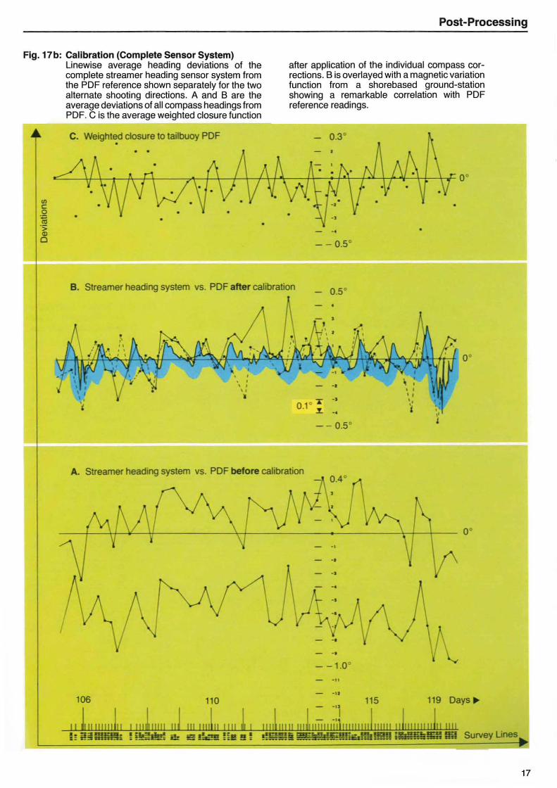
Fig. 17b: Calibration (Complete Sensor System) Linewise average heading deviations of the complete streamer heading sensor system from the PDF reference shown separately for the two alternate shooting directions. A and Bare the average deviations of all compass headings from PDF. C is the average weighted closure function

C. Weight~ ctosure to tailbuoy PDF

after application of the individual compass cor­rections. Bis overlayed with a magnetic variation function from a shorebased ground-station showing a remarkable correlation with PDF reference readings.

- -, _ - 0.50

B. Streamer heading system vs. PDF after calibration

- .

- - 0.50

A. Streamer heading system VS. PDF before caJibration

o

- ... - - I

- -1 .0 -u

-I. 106 110 115 119 Days .

Survey Unes

17

Post-Processing

18

, .\

,.~ "". E_ ............. __ W_E.::.eI_G_H_T_E_D_C_LJ.~~S_U_R_E_F_U_.JC!....-TIO __ ~ I 4.IB.ft: P\JIC.

Fig. 17 c: Final Sensor Plot (with closure function to PDF)

, ~n4 r-

! t t las " . Jaa t t t ! I

•

SENSOR CORRELATION

Fig.18a: Sensor Correlation and Streamer Shape

Determination Technique

NORMAL TIM E WINO OW HEAD' os

REMARKS TIME LAG WINOOW HeAOIH'S

• • ~O~ I(A'UII'

I • COM"ASS

•• CO M,.A55

• CO""AS5

•• CO"'A55

•• CO"'A55

• CO""A$$

,. (O .. 'ASS

1. CO .. 'AS5

I. CO .. 'A55

C. OfPAIfIUIIlE A .. GlE

G. GYRO

10W I'OI N1

f". CON'ASS

• CORRIELATIO ..

t~ ___ INTERPOLATION ~~----"';":':'-':":':":': ' -2

t

•

CORRIELATIO C

G

INS'AIIT. '0511 10111

STREAMER SHAPE DETERMINATION

N N

H ..... --1t---4~"*~ 'AllellOY

JIIO eO"PA55

lllD CO .. 'ASS

• -TII co..,,,ss , .. alN'.SS

Post-Processing

400 315 350

1, I POP TRACK j~ 325 ~~, IC X, lIf ... )C I POP • ... ,----x-

"""" " x " ... ....

SCALE b3 E3 F=I ----' y~y .... y---- ---- -___ ' y .... .::...y-

O.5KM TAILBUOY TRACK --- '---

\ TAILBUOY

Fig. 18b: Weigthed Closure 01 the Streamer Shape Function to PDF

Fig. 19: Subsurface Scattergram

__ ; ö

" t . ..... ---r . -.- --' . !o

"

' " ' .. - ; . -.. ;;.t = "

19

f\ PRAKlA 5E15MD5

\J V

BIN COVERAGE

Bin coverage displays for all offsets includlng overfill.

PRAKLA-SEISMOS GMBH· BUCHHOLZER STR. 100 . P.O.B. 51 0530 0-3000 HANNOVER 51 . FEOERAL REPUBLIC OF GERMANY

"bo". 80. 0 55. 0- 80. 0 50. 0- 55. 0 45. 0- 50. 0 40. 0- '5 . 0 35. 0- '0. 0 30. 0- 35. 0 25. 0- 30. 0 20.0- 25. 0 16. 0- 20. 0 10. 0- 15. 0 5. 0 - 10. 0 1. 0 - 5 . 0

below l. 0

PHONE: (511) 6420 . TELEX: 922847 + 922419 + 923250 . CABLE: PRAKLA GERMANY

© Copyright PRAKLA-SEISMOS GMBH

50001184