praise for cuda for engineers -...
TRANSCRIPT


PRAISE FOR CUDA FOR ENGINEERS
“First there was FORTRAN, circa 1960, which enabled us to program main-frames. Then there was BASIC, circa 1980, which enabled us to program the first microcomputers. And now there is CUDA, which enables us to program super-microcomputers.
“CUDA for Engineers allows researchers in engineering and mathematics to perform calculations hundreds of times faster than was previously possible on microcomputers. This permits new kinds of calculations to be performed and reveals this book to be a game changer.”
— Richard H. Rand, professor of mechanical and aerospace engineering, and of mathematics, Cornell University
“CUDA for Engineers has been put together in a very thoughtful and practical way. The reader is quickly immersed in the world of parallel programming with CUDA and results are seen right away. This book is a great introduction and helps readers from many different scientific and engineering disciplines become exposed to the benefits of GPU programming. This book is an enjoyable read and has great support through top-notch example programs and exercises.”
— Dr. Mark Staveley, senior program manager, Azure High Performance Computing
“CUDA for Engineers lives up to its name by stepping the reader through con-cepts, strategies, terminology, and examples, which work together to form an educational framework so that experts and non-experts alike can approach high- performance computing with foresight and understanding.”
— Joseph M. Iaquinto, Ph.D., research specialist, VA Puget Sound
“This book reflects a practical approach that is in perfect agreement with the way I teach numerical methods for engineers. It would make a fine supplement for engineering students or practitioners to add CUDA to their numerical tool-box, and thus embark on the study of high-performance scientific computing. It’s perfect for newcomers to CUDA who already have a foundation in program-ming. I recommend following the authors’ advice and working immediately with the hands-on exercis es, step by step. After this immersion, you will approach proficiency by simply adding some personal projects in GPU computing and delving into the NVIDIA CUDA Guide and developer community.”
— Lorena A. Barba, associate professor of mechanical and aerospace engineering, The George Washington University
This page intentionally left blank

CUDA for Engineers

This page intentionally left blank

CUDA for EngineersAn Introduction to High-Performance Parallel Computing
Duane StortiMete Yurtoglu
New York • Boston • Indianapolis • San FranciscoToronto • Montreal • London • Munich • Paris • MadridCapetown • Sydney • Tokyo • Singapore • Mexico City

Many of the designations used by manufacturers and sellers to distinguish their products are claimed as trademarks. Where those designations appear in this book, and the publisher was aware of a trademark claim, the designations have been printed with initial capital letters or in all capitals.
The authors and publisher have taken care in the preparation of this book, but make no expressed or implied warranty of any kind and assume no responsibility for errors or omissions. No liability is assumed for incidental or consequential damages in connection with or arising out of the use of the information or programs contained herein.
For information about buying this title in bulk quantities, or for special sales opportunities (which may include electronic versions; custom cover designs; and content particular to your business, training goals, marketing focus, or branding interests), please contact our corporate sales department at [email protected] or (800) 382-3419.
For government sales inquiries, please contact [email protected].
For questions about sales outside the U.S., please contact [email protected].
Visit us on the Web: informit.com/aw
Library of Congress Cataloging-in-Publication Data
Names: Storti, Duane, author. | Yurtoglu, Mete.Title: CUDA for engineers : an introduction to high-performance parallel computing / Duane Storti, Mete Yurtoglu.Description: New York : Addison-Wesley, 2015. | Includes bibliographical references and index.Identifiers: LCCN 2015034266 | ISBN 9780134177410 (pbk. : alk. paper)Subjects: LCSH: Parallel computers. | CUDA (Computer architecture)Classification: LCC QA76.58 .S76 2015 | DDC 004/.35—dc23LC record available at http://lccn.loc.gov/2015034266
Copyright © 2016 Pearson Education, Inc.
All rights reserved. Printed in the United States of America. This publication is protected by copyright, and permission must be obtained from the publisher prior to any prohibited reproduction, storage in a retrieval system, or transmission in any form or by any means, electronic, mechanical, photocopying, recording, or likewise. To obtain permission to use material from this work, please submit a written request to Pearson Education, Inc., Permissions Department, 200 Old Tappan Road, Old Tappan, New Jersey 07675, or you may fax your request to (201) 236-3290.
NVIDIA, the NVIDIA logo, CUDA, GeForce GeForce GTX, Jetson, Kepler, NVIDIA Maxwell, Nsight, Optimus, Pascal, Quadro, and Tesla are trademarks and/or registered trademarks of NVIDIA Corporation in the U.S. and/or other countries.
Microsoft, Visual Studio, and Windows are trademarks of the Microsoft group of companies.
Apple, the Apple logo, Mac, OpenCL, and OS X are trademarks of Apple Inc., registered in the U.S. and other countries.
Intel and Intel Core are trademarks of Intel Corporation in the U.S. and other countries.
ArrayFire and the ArrayFire logo are trademarks of ArrayFire LLC.
UNIX is a registered trademark of The Open Group.
Wikipedia is a registered trademark of the Wikimedia Foundation, Inc.
IBM, Blue Gene, and PowerPC are trademarks of International Business Machines Corp., registered in many jurisdictions worldwide.
UNIX is a registered trademark of The Open Group in the United States and other countries.
Linux is a registered trademark of Linus Torvalds in the United States, other countries, or both.
ISBN-13: 978-0-13-417741-0ISBN-10: 0-13-417741-XText printed in the United States on recycled paper at RR Donnelley in Crawfordsville, Indiana.First printing, November 2015
Editor-in-ChiefMark L. Taub
Executive EditorLaura Lewin
Development EditorSonglin Qiu
Managing EditorJohn Fuller
Project EditorElizabeth Ryan
Copy EditorTeresa Barensfeld
IndexerJack Lewis
ProofreaderAnna Popick
Technical ReviewersTom BradleyRichard RandMark Staveley
Editorial AssistantOlivia Basegio
Cover DesignerChuti Prasertsith
CompositorThe CIP Group

To the family, friends, and teachers who inspire us to keep learning cool things
and to share what we have learned.

This page intentionally left blank

ix
Contents
Acknowledgments . . . . . . . . . . . . . . . . . . . . . . . . . . . . . . . . xvii
About the Authors . . . . . . . . . . . . . . . . . . . . . . . . . . . . . . . . . xix
Introduction . . . . . . . . . . . . . . . . . . . . . . . . . . . . . . 1
What Is CUDA? . . . . . . . . . . . . . . . . . . . . . . . . . . . . . . . . . . . . 1
What Does “Need-to-Know” Mean for Learning CUDA? . . . . . . . . . . . . 2
What Is Meant by “for Engineers”? . . . . . . . . . . . . . . . . . . . . . . . . 3
What Do You Need to Get Started with CUDA? . . . . . . . . . . . . . . . . . . 4
How Is This Book Structured? . . . . . . . . . . . . . . . . . . . . . . . . . . . 4
Conventions Used in This Book . . . . . . . . . . . . . . . . . . . . . . . . . . . 8
Code Used in This Book . . . . . . . . . . . . . . . . . . . . . . . . . . . . . . . 8
User’s Guide . . . . . . . . . . . . . . . . . . . . . . . . . . . . . . . . . . . . . 9
Historical Context . . . . . . . . . . . . . . . . . . . . . . . . . . . . . . . . . 10
References . . . . . . . . . . . . . . . . . . . . . . . . . . . . . . . . . . . . . 12
Chapter 1: First Steps . . . . . . . . . . . . . . . . . . . . . . . 13
Running CUDA Samples . . . . . . . . . . . . . . . . . . . . . . . . . . . . . 13
CUDA Samples under Windows . . . . . . . . . . . . . . . . . . . . . . . . 14
CUDA Samples under Linux . . . . . . . . . . . . . . . . . . . . . . . . . . 17
Estimating “Acceleration” . . . . . . . . . . . . . . . . . . . . . . . . . . . 17

x
CONTENTS
Running Our Own Serial Apps . . . . . . . . . . . . . . . . . . . . . . . . . . 19
dist_v1 . . . . . . . . . . . . . . . . . . . . . . . . . . . . . . . . . . . . . 19
dist_v2 . . . . . . . . . . . . . . . . . . . . . . . . . . . . . . . . . . . . . 20
Summary . . . . . . . . . . . . . . . . . . . . . . . . . . . . . . . . . . . . . . 22
Suggested Projects . . . . . . . . . . . . . . . . . . . . . . . . . . . . . . . . 23
Chapter 2: CUDA Essentials . . . . . . . . . . . . . . . . . . . 25
CUDA’s Model for Parallelism . . . . . . . . . . . . . . . . . . . . . . . . . . 25
Need-to-Know CUDA API and C Language Extensions . . . . . . . . . . . . 28
Summary . . . . . . . . . . . . . . . . . . . . . . . . . . . . . . . . . . . . . . 31
Suggested Projects . . . . . . . . . . . . . . . . . . . . . . . . . . . . . . . . 31
References . . . . . . . . . . . . . . . . . . . . . . . . . . . . . . . . . . . . . 31
Chapter 3: From Loops to Grids . . . . . . . . . . . . . . . . . 33
Parallelizing dist_v1 . . . . . . . . . . . . . . . . . . . . . . . . . . . . . . 33
Executing dist_v1_cuda . . . . . . . . . . . . . . . . . . . . . . . . . . 37
Parallelizing dist_v2 . . . . . . . . . . . . . . . . . . . . . . . . . . . . . . 38
Standard Workflow . . . . . . . . . . . . . . . . . . . . . . . . . . . . . . . . 42
Simplified Workflow . . . . . . . . . . . . . . . . . . . . . . . . . . . . . . . . 43
Unified Memory and Managed Arrays . . . . . . . . . . . . . . . . . . . . 43
Distance App with cudaMallocManaged() . . . . . . . . . . . . . . . . 44
Summary . . . . . . . . . . . . . . . . . . . . . . . . . . . . . . . . . . . . . . 47
Suggested Projects . . . . . . . . . . . . . . . . . . . . . . . . . . . . . . . . 48
References . . . . . . . . . . . . . . . . . . . . . . . . . . . . . . . . . . . . . 48
Chapter 4: 2D Grids and Interactive Graphics . . . . . . . . . 49
Launching 2D Computational Grids . . . . . . . . . . . . . . . . . . . . . . . 50
Syntax for 2D Kernel Launch . . . . . . . . . . . . . . . . . . . . . . . . . 51

CONTENTS
xi
Defining 2D Kernels . . . . . . . . . . . . . . . . . . . . . . . . . . . . . . 52
dist_2d . . . . . . . . . . . . . . . . . . . . . . . . . . . . . . . . . . . . . 53
Live Display via Graphics Interop . . . . . . . . . . . . . . . . . . . . . . . . 56
Application: Stability . . . . . . . . . . . . . . . . . . . . . . . . . . . . . . . . 66
Running the Stability Visualizer . . . . . . . . . . . . . . . . . . . . . . . . 73
Summary . . . . . . . . . . . . . . . . . . . . . . . . . . . . . . . . . . . . . . 76
Suggested Projects . . . . . . . . . . . . . . . . . . . . . . . . . . . . . . . . 76
References . . . . . . . . . . . . . . . . . . . . . . . . . . . . . . . . . . . . . 77
Chapter 5: Stencils and Shared Memory . . . . . . . . . . . . 79
Thread Interdependence . . . . . . . . . . . . . . . . . . . . . . . . . . . . . 80
Computing Derivatives on a 1D Grid . . . . . . . . . . . . . . . . . . . . . . . 81
Implementing dd_1d_global . . . . . . . . . . . . . . . . . . . . . . . . 82
Implementing dd_1d_shared . . . . . . . . . . . . . . . . . . . . . . . . 85
Solving Laplace’s Equation in 2D: heat_2d . . . . . . . . . . . . . . . . . 88
Sharpening Edges in an Image: sharpen . . . . . . . . . . . . . . . . . 102
Summary . . . . . . . . . . . . . . . . . . . . . . . . . . . . . . . . . . . . . 117
Suggested Projects . . . . . . . . . . . . . . . . . . . . . . . . . . . . . . . 118
References . . . . . . . . . . . . . . . . . . . . . . . . . . . . . . . . . . . . 119
Chapter 6: Reduction and Atomic Functions . . . . . . . . . . 121
Threads Interacting Globally . . . . . . . . . . . . . . . . . . . . . . . . . . 121
Implementing parallel_dot . . . . . . . . . . . . . . . . . . . . . . . . . 123
Computing Integral Properties: centroid_2d . . . . . . . . . . . . . . . 130
Summary . . . . . . . . . . . . . . . . . . . . . . . . . . . . . . . . . . . . . 138
Suggested Projects . . . . . . . . . . . . . . . . . . . . . . . . . . . . . . . 138
References . . . . . . . . . . . . . . . . . . . . . . . . . . . . . . . . . . . . 138

xii
CONTENTS
Chapter 7: Interacting with 3D Data . . . . . . . . . . . . . . . 141
Launching 3D Computational Grids: dist_3d . . . . . . . . . . . . . . . . 144
Viewing and Interacting with 3D Data: vis_3d . . . . . . . . . . . . . . . 146
Slicing . . . . . . . . . . . . . . . . . . . . . . . . . . . . . . . . . . . . . 149
Volume Rendering . . . . . . . . . . . . . . . . . . . . . . . . . . . . . . 153
Raycasting . . . . . . . . . . . . . . . . . . . . . . . . . . . . . . . . . . . 154
Creating the vis_3d App . . . . . . . . . . . . . . . . . . . . . . . . . . 156
Summary . . . . . . . . . . . . . . . . . . . . . . . . . . . . . . . . . . . . . 171
Suggested Projects . . . . . . . . . . . . . . . . . . . . . . . . . . . . . . . 171
References . . . . . . . . . . . . . . . . . . . . . . . . . . . . . . . . . . . . 171
Chapter 8: Using CUDA Libraries . . . . . . . . . . . . . . . . 173
Custom versus Off-the-Shelf . . . . . . . . . . . . . . . . . . . . . . . . . . 173
Thrust . . . . . . . . . . . . . . . . . . . . . . . . . . . . . . . . . . . . . . . 175
Computing Norms with inner_product() . . . . . . . . . . . . . . . 176
Computing Distances with transform() . . . . . . . . . . . . . . . . 180
Estimating Pi with generate(), transform(), and reduce() . . . 185
cuRAND . . . . . . . . . . . . . . . . . . . . . . . . . . . . . . . . . . . . . . 190
NPP . . . . . . . . . . . . . . . . . . . . . . . . . . . . . . . . . . . . . . . . 193
sharpen_npp . . . . . . . . . . . . . . . . . . . . . . . . . . . . . . . . 194
More Image Processing with NPP . . . . . . . . . . . . . . . . . . . . . 198
Linear Algebra Using cuSOLVER and cuBLAS . . . . . . . . . . . . . . . . 201
cuDNN . . . . . . . . . . . . . . . . . . . . . . . . . . . . . . . . . . . . . . . 207
ArrayFire . . . . . . . . . . . . . . . . . . . . . . . . . . . . . . . . . . . . . 207
Summary . . . . . . . . . . . . . . . . . . . . . . . . . . . . . . . . . . . . . 207
Suggested Projects . . . . . . . . . . . . . . . . . . . . . . . . . . . . . . . 208
References . . . . . . . . . . . . . . . . . . . . . . . . . . . . . . . . . . . . 209

CONTENTS
xiii
Chapter 9: Exploring the CUDA Ecosystem . . . . . . . . . . . 211
The Go-To List of Primary Sources . . . . . . . . . . . . . . . . . . . . . . 211
CUDA Zone . . . . . . . . . . . . . . . . . . . . . . . . . . . . . . . . . . 211
Other Primary Web Sources . . . . . . . . . . . . . . . . . . . . . . . . 212
Online Courses . . . . . . . . . . . . . . . . . . . . . . . . . . . . . . . . 213
CUDA Books . . . . . . . . . . . . . . . . . . . . . . . . . . . . . . . . . . 214
Further Sources . . . . . . . . . . . . . . . . . . . . . . . . . . . . . . . . . 217
CUDA Samples . . . . . . . . . . . . . . . . . . . . . . . . . . . . . . . . 217
CUDA Languages and Libraries . . . . . . . . . . . . . . . . . . . . . . 217
More CUDA Books . . . . . . . . . . . . . . . . . . . . . . . . . . . . . . 217
Summary . . . . . . . . . . . . . . . . . . . . . . . . . . . . . . . . . . . . . 218
Suggested Projects . . . . . . . . . . . . . . . . . . . . . . . . . . . . . . . 219
Appendix A: Hardware Setup . . . . . . . . . . . . . . . . . . . 221
Checking for an NVIDIA GPU: Windows . . . . . . . . . . . . . . . . . . . . 221
Checking for an NVIDIA GPU: OS X . . . . . . . . . . . . . . . . . . . . . . 222
Checking for an NVIDIA GPU: Linux . . . . . . . . . . . . . . . . . . . . . . 223
Determining Compute Capability . . . . . . . . . . . . . . . . . . . . . . . 223
Upgrading Compute Capability . . . . . . . . . . . . . . . . . . . . . . . . . 225
Mac or Notebook Computer with a CUDA-Enabled GPU . . . . . . . . . 225
Desktop Computer . . . . . . . . . . . . . . . . . . . . . . . . . . . . . . 226
Appendix B: Software Setup . . . . . . . . . . . . . . . . . . 229
Windows Setup . . . . . . . . . . . . . . . . . . . . . . . . . . . . . . . . . . 229
Creating a Restore Point . . . . . . . . . . . . . . . . . . . . . . . . . . . 230
Installing the IDE . . . . . . . . . . . . . . . . . . . . . . . . . . . . . . . 230
Installing the CUDA Toolkit . . . . . . . . . . . . . . . . . . . . . . . . . 230
Initial Test Run . . . . . . . . . . . . . . . . . . . . . . . . . . . . . . . . 235

xiv
CONTENTS
OS X Setup . . . . . . . . . . . . . . . . . . . . . . . . . . . . . . . . . . . . 238
Downloading and Installing the CUDA Toolkit . . . . . . . . . . . . . . . 239
Linux Setup . . . . . . . . . . . . . . . . . . . . . . . . . . . . . . . . . . . . 240
Preparing the System Software for CUDA Installation . . . . . . . . . . 240
Downloading and Installing the CUDA Toolkit . . . . . . . . . . . . . . . 240
Installing Samples to the User Directory . . . . . . . . . . . . . . . . . 241
Initial Test Run . . . . . . . . . . . . . . . . . . . . . . . . . . . . . . . . 242
Appendix C: Need-to-Know C Programming . . . . . . . . . 245
Characterization of C . . . . . . . . . . . . . . . . . . . . . . . . . . . . . . 245
C Language Basics . . . . . . . . . . . . . . . . . . . . . . . . . . . . . . . 246
Data Types, Declarations, and Assignments . . . . . . . . . . . . . . . . . 248
Defining Functions . . . . . . . . . . . . . . . . . . . . . . . . . . . . . . . . 250
Building Apps: Create, Compile, Run, Debug . . . . . . . . . . . . . . . . . 251
Building Apps in Windows . . . . . . . . . . . . . . . . . . . . . . . . . . 252
Building Apps in Linux . . . . . . . . . . . . . . . . . . . . . . . . . . . . 258
Arrays, Memory Allocation, and Pointers . . . . . . . . . . . . . . . . . . . 262
Control Statements: for, if . . . . . . . . . . . . . . . . . . . . . . . . . . 263
The for Loop . . . . . . . . . . . . . . . . . . . . . . . . . . . . . . . . . 264
The if Statement . . . . . . . . . . . . . . . . . . . . . . . . . . . . . . . 265
Other Control Statements . . . . . . . . . . . . . . . . . . . . . . . . . . 267
Sample C Programs . . . . . . . . . . . . . . . . . . . . . . . . . . . . . . . 267
dist_v1 . . . . . . . . . . . . . . . . . . . . . . . . . . . . . . . . . . . . 267
dist_v2 . . . . . . . . . . . . . . . . . . . . . . . . . . . . . . . . . . . . 271
dist_v2 with Dynamic Memory . . . . . . . . . . . . . . . . . . . . . . 275
References . . . . . . . . . . . . . . . . . . . . . . . . . . . . . . . . . . . . 277

CONTENTS
xv
Appendix D: CUDA Practicalities: Timing, Profiling, Error Handling, and Debugging . . . . . . . . . 279
Execution Timing and Profiling . . . . . . . . . . . . . . . . . . . . . . . . . 279
Standard C Timing Methods . . . . . . . . . . . . . . . . . . . . . . . . . 280
CUDA Events . . . . . . . . . . . . . . . . . . . . . . . . . . . . . . . . . 282
Profiling with NVIDIA Visual Profiler . . . . . . . . . . . . . . . . . . . . 284
Profiling in Nsight Visual Studio . . . . . . . . . . . . . . . . . . . . . . 288
Error Handling . . . . . . . . . . . . . . . . . . . . . . . . . . . . . . . . . . 292
Debugging in Windows . . . . . . . . . . . . . . . . . . . . . . . . . . . . . 298
Debugging in Linux . . . . . . . . . . . . . . . . . . . . . . . . . . . . . . . 305
CUDA-MEMCHECK . . . . . . . . . . . . . . . . . . . . . . . . . . . . . . . 308
Using Visual Studio Property Pages . . . . . . . . . . . . . . . . . . . . . . 309
References . . . . . . . . . . . . . . . . . . . . . . . . . . . . . . . . . . . . 312
Index . . . . . . . . . . . . . . . . . . . . . . . . . . . . . . . . . . . . . . . . 313

This page intentionally left blank

xvii
Acknowledgments
The authors wish to express their thanks to a variety of people without whom this book would never have come into existence.
Thank you to all the family members who received a bit less attention while we were consumed by the writing of this book. Thank you to Laura Lewin and everyone at Pearson who contributed to the editing, production, and marketing efforts. Thank you to Nicholas Wilt (formerly at NVIDIA and currently at Ama-zon), who first put us in contact with Laura and really got the ball rolling. Thanks also to our technical reviewers Thomas Bradley of NVIDIA, Mark Staveley of Microsoft, and Richard Rand of Cornell University, all of whom provided helpful comments, corrections, and insights.
Thank you to the many colleagues here at the University of Washington–Seattle Department of Mechanical Engineering who contributed via discussions rang-ing from big-picture perspective down to the finest technical details. That list includes but is not limited to Mark Ganter, Di Zhang, and Ben Weiss (who helped create several of the figures and also provided us with some lifesaving software to support logical tags and automated code formatting). We would also like to thank Mechanical Engineering Department Chair Per Reinhall for his approval for us to offer the class that helped to inspire the creation of much of the book’s content. Additional thanks go to our colleagues David Haynor of University of Washington Department of Radiology and William Ledoux of the Seattle VA Hos-pital, whose research initiatives continue to motivate meaningful journeys into CUDA territory.
We wish to say a special thank you to the good folks at NVIDIA, including CEO Jen-Hsun Huang who not only had, but also acted on, a vision of what could be accomplished by enhancing access to GPU-based parallel computing; Chandra Cheij, Academic Programs Manager; Kimberly Powell, Director of Higher Edu-cation and Healthcare Industries; Jon Saposhnik and Bob Crovella, helpful and inspirational CUDA gurus; and last, but definitely not least, Jay White, Director

ACKNOWLEDGMENTS
xviii
of Strategic Marketing, who sustains the Seattle-area GPU-computing meet-up group and serves as our local go-to guy.
We would also like to thank all the students who had the sense of adventure to participate in the initial CUDA-based class offerings at the University of Wash-ington, especially former ME graduate student Grant Marchelli (now Grant Marchelli, Ph.D., CTO of Envitrum Inc.), who played a key role in everything from setting up the lab to providing code samples and delivering guest lectures. A special thank you goes to Gerald Barnett, who was so generous with his time and expertise when it came time to edit the first draft.
Finally, a big thanks to you, the reader. The value of having something important to share depends on having people to share it with; we appreciate your inter-est, and we sincerely hope this book provides you with useful and productive experiences.

xix
About the Authors
Duane Storti received a Ph.D. in theoretical and applied mechanics from Cornell University in 1984. Since then, he has served as a professor of mechanical engineering at the University of Washington–Seattle. Duane has 35 years of experience in teaching and research in the areas of engineering mathematics, dynamics and vibrations, computer-aided design, 3D printing, and applied GPU computing. When not on campus, he can often be found in the gym, coaching youth volleyball.
Mete Yurtoglu received a B.S. in physics and a B.S. in mechanical engineering in 2008, and an M.S. in 2011 from Bogazici University in Istanbul, Turkey. He is currently a graduate student at the University of Washington–Seattle pur-suing an M.S. in applied mathematics and a Ph.D. in mechanical engineering. His research interests focus on GPU-based methods for computer vision and machine learning. Mete enjoys family time, playing soccer, and working out.

This page intentionally left blank

49
Chapter 4
2D Grids and Interactive Graphics
In this chapter, we see that the CUDA model of parallelism extends readily to two dimensions (2D). We go through the basics of launching a 2D computational grid and create a skeleton kernel you can use to compute a 2D grid of values for functions of interest to you. We then specialize the kernel to create dist_2d, an app that computes the distance from a reference point in the plane to each member of a uniform 2D grid of points. By identifying the grid of points with pixels in an image, we compute data for an image whose shading is based on distance values.
Once we are generating image data, it is only natural to take advantage of CUDA’s graphics interoperability (or graphics interop for short) capability, which supports cooperation with standard graphics application programming interfaces (APIs) including Direct3D [1] and OpenGL [2]. We’ll use OpenGL, and maintaining our need-to-know approach, we’ll very quickly provide just the necessities of OpenGL to get your results on the screen at interactive speeds.
By the end of this chapter you will have run a flashlight app that interactively displays an image with shading based on distance from a reference point that you can move using mouse or keyboard input and a stability app that inter-actively displays the results of several hundred thousand numerical simulations of the dynamics of an oscillator. This experience should get you to the point where you are ready to start creating your own CUDA-powered interactive apps.

CHAPTER 4 2D GRIDS AND INTERACTIVE GRAPHICS
50
Launching 2D Computational GridsHere we expand on our earlier examples that involved a 1D array (points dis-tributed regularly along a line segment) and move on to consider applications involving points regularly distributed on a portion of a 2D plane. While we will encounter other applications (e.g., simulating heat conduction) that fit this scenario, the most common (and likely most intuitive) example involves digital image processing. To take advantage of the intuitive connection, we will use image-processing terminology in presenting the concepts—all of which will transfer directly to other applications.
A digital raster image consists of a collection of picture elements or pixels arranged in a uniform 2D rectangular grid with each pixel having a quantized intensity value. To be concrete, let’s associate the width and height directions with the x and y coordinates, respectively, and say that our image is W pixels wide by H pixels high. If the quantized value stored in each pixel is simply a number, the data for an image matches exactly with the data for a matrix of size W x H.
As we move on from 1D to 2D problems in CUDA, we hope you will be pleasantly surprised by how few adjustments need to be made. In 1D, we specified integer values for block and grid sizes and computed an index i based on blockDim.x, blockIdx.x, and threadIdx.x according to the formula
int i = blockIdx.x*blockDim.x + threadIdx.x;
Here we reinterpret the expression on the right-hand side of the assignment as the specification of a new index c that keeps track of what column each pixel belongs to. (As we traverse a row of pixels from left to right, c increases from its minimum value 0 to its maximum value W-1.) We also introduce a second index r to keep track of row numbers (ranging from 0 to H-1). The row index is computed just as the column index is, but using the .y components (instead of the .x components), so the column and row indices are computed as follows:
int c = blockIdx.x*blockDim.x + threadIdx.x;int r = blockIdx.y*blockDim.y + threadIdx.y;
To keep data storage and transfer simple, we will continue to store and trans-fer data in a “flat” 1D array, so we will have one more integer variable to index into the 1D array. We will continue to call that variable i, noting that i played this role in the 1D case, but in other places (including the CUDA Samples) you will see variables named idx, flatIdx, and offset indexing the 1D array. We place values in the 1D array in row major order—that is, by storing the data from

LAUNCHING 2D COMPUTATIONAL GRIDS
51
row 0, followed by the data from row 1, and so on—so the index i in the 1D array is now computed as follows:
int i = r*w + c;
To describe the 2D computational grid that intuitively matches up with an image (or matrix or other regular 2D discretization), we specify block and grid sizes using dim3 variables with two nontrivial components. Recall that an integer within the triple chevrons of a kernel call is treated as the .x component of a dim3 variable with a default value of 1 for the unspecified .y and .z components. In the current 2D context, we specify nontrivial .x and .y components. The .z component of the dim3, which here has the default value 1, will come into play when we get to 3D grids in Chapter 7, “Interacting with 3D Data.”
Without further ado, let’s lay out the necessary syntax and get directly to parallel computation of pixel values with a 2D grid.
SYNTAX FOR 2D KERNEL LAUNCH
The 2D kernel launch differs from the 1D launch only in terms of the execution configuration. Computing data for an image involves W columns and H rows, and we can organize the computation into 2D blocks with TX threads in the x-direction and TY threads in the y-direction. (You can choose to organize your 2D grid into 1D blocks, but you will run into limits on both maximum block dimension and total number of threads in a block. See the CUDA C Programming Guide [3] for details.)
We specify the 2D block size with a single statement:
dim3 blockSize(TX, TY); // Equivalent to dim3 blockSize(TX, TY, 1);
and then we compute the number of blocks (bx and by) needed in each direction exactly as in the 1D case.
int bx = (W + blockSize.x - 1)/blockSize.x ;int by = (H + blockSize.y – 1)/blockSize.y ;
The syntax for specifying the grid size (in blocks) is
dim3 gridSize = dim3(bx, by);
With those few details in hand, we are ready to launch:
kernelName<<<gridSize, blockSize>>>(args)

CHAPTER 4 2D GRIDS AND INTERACTIVE GRAPHICS
52
DEFINING 2D KERNELS
The prototype or declaration of a kernel to be launched on a 2D grid will look exactly as before: it starts with the qualifier __global__ followed by return type void and a legal name, such as kernel2D, and ends with a comma- separated list of typed arguments (which better include a pointer to a device array d_out where the computed image data will be stored, along with the width and height of the image and any other required inputs). The kernel2D function begins by computing the row, column, and flat indices and testing that the row and column indices have values corresponding to a pixel within the image. All that is left is computing the value for the pixel.
Putting the pieces together, the structure of a typical 2D kernel is given in Listing 4.1.
Listing 4.1 “Skeleton” listing for a kernel to be launched on a 2D grid. Replace INSERT_CODE_HERE with your code for computing the output value. 1 __global__ 2 void kernel2D(float *d_out, int w, int h, … ) 3 { 4 // Compute column and row indices. 5 const int c = blockIdx.x * blockDim.x + threadIdx.x; 6 const int r = blockIdx.y * blockDim.y + threadIdx.y; 7 const int i = r * w + c; // 1D flat index 8 9 // Check if within image bounds. 10 if ((c >= w) || (r >= h)) 11 return; 12 13 d_out[i] = INSERT_CODE_HERE; // Compute/store pixel in device array. 14 }
A Note on Capitalization of Variable NamesWe need to refer to parameter values such as the width and height of an image inside of function definitions where they are considered as input variables, but the input value in the function call will typically be a constant value specified using #define. We will follow the prevailing convention by using uppercase for the con-stant value and the same name in lowercase for the input variable. For example, the function kernel2D() in Listing 4.1 has the prototype
void kernel2D(uchar4 *d_out, int w, int h, … )
and the function call

LAUNCHING 2D COMPUTATIONAL GRIDS
53
#define W 500#define H 500kernel2D<<<gridSize, blockSize>>>(d_out, W, H, … )
indicates that the input values for width and height are constants, here with value 500.
One detail worth dealing with at this point is a common data type for images. The quantized value stored for each pixel is of type uchar4, which is a vector type storing four unsigned character values (each of which occupies 1 byte of storage). For practical purposes, you can think of the four components of the uchar4 (designated as usual by suffixes .x, .y, .z, and .w) as specifying integer values ranging from 0 to 255 for the red, green, blue, and alpha (opacity) display channels. This format for describing pixel values in an image is often abbreviated as RGBA.
Putting the pieces together, the structure of a typical 2D kernel for computing an image is given in Listing 4.2.
Listing 4.2 “Skeleton” listing for computing data for an image. RED_FORMULA, GREEN_FORMULA, and BLUE_FORMULA should be replaced with your code for computing desired val-ues between 0 and 255 for each color channel. 1 __global__ 2 void kernel2D(uchar4 *d_output, int w, int h, … ) 3 { 4 // Compute column and row indices. 5 int c = blockIdx.x*blockDim.x + threadIdx.x; 6 int r = blockIdx.y*blockDim.y + threadIdx.y; 7 int i = r * w + c; // 1D flat index 8 9 // Check if within image bounds. 10 if ((r >= h) || (c >= w)) { 11 return; 12 } 13 14 d_output[i].x = RED_FORMULA; //Compute red 15 d_output[i].y = GREEN_ FORMULA; //Compute green 16 d_output[i].z = BLUE_ FORMULA; //Compute blue 17 d_output[i].w = 255; // Fully opaque 18 }
dist_2d
Let’s tie the general discussion of 2D grids together with our earlier exam-ples involving distance apps by coding up an app that produces a 2D array of distances from a reference point, and then we’ll adapt the app to produce an

CHAPTER 4 2D GRIDS AND INTERACTIVE GRAPHICS
54
array of data for an RGBA image. Listing 4.3 provides all the code for computing distances on a 2D grid.
Listing 4.3 Computing distances on a 2D grid 1 #define W 500 2 #define H 500 3 #define TX 32 // number of threads per block along x-axis 4 #define TY 32 // number of threads per block along y-axis 5 6 __global__ 7 void distanceKernel(float *d_out, int w, int h, float2 pos) 8 { 9 const int c = blockIdx.x*blockDim.x + threadIdx.x; 10 const int r = blockIdx.y*blockDim.y + threadIdx.y; 11 const int i = r*w + c; 12 if ((c >= w) || (r >= h)) return; 13 14 // Compute the distance and set d_out[i] 15 d_out[i] = sqrtf((c - pos.x)*(c - pos.x) + 16 (r - pos.y)*(r - pos.y)); 17 } 18 19 int main() 20 { 21 float *out = (float*)calloc(W*H, sizeof(float)); 22 float *d_out; // pointer for device array 23 cudaMalloc(&d_out, W*H*sizeof(float)); 24 25 const float2 pos = {0.0f, 0.0f}; // set reference position 26 const dim3 blockSize(TX, TY); 27 const int bx = (W + TX - 1)/TX; 28 const int by = (W + TY - 1)/TY; 29 const dim3 gridSize = dim3(bx, by); 30 31 distanceKernel<<<gridSize, blockSize>>>(d_out, W, H, pos); 32 33 // Copy results to host. 34 cudaMemcpy(out, d_out, W*H*sizeof(float), cudaMemcpyDeviceToHost); 35 36 cudaFree(d_out); 37 free(out); 38 return 0; 39 }
The kernel, lines 6–17, is exactly as in Listing 4.1 but with a result computed using the Pythagorean formula to compute the distance between the location {c, r} and a reference location pos. (Note that we have defined pos to have type float2 so it can store both coordinates of the reference location {pos.x, pos.y}.) The rest of the listing, lines 19–39, gives the details of main() starting with declaration of an output array of appropriate size initialized to zero. Lines

LAUNCHING 2D COMPUTATIONAL GRIDS
55
22–23 declare a pointer to the device array d_out and allocate the memory with cudaMalloc(). Line 25 sets the reference position, and lines 26–29 set the kernel launch parameters: a 2D grid of bx × by blocks each having TX × TY threads. Line 31 launches the kernel to compute the distance values, which are copied back to out on the host side on line 34. Lines 36–37 free the allocated device and host memory, then main() returns zero to indicate completion.
Next we make a few minor changes to produce an app that computes an array of RGBA values corresponding to a distance image. The full code is provided in Listing 4.4.
Listing 4.4 Parallel computation of image data based on distance from a reference point in 2D 1 #define W 500 2 #define H 500 3 #define TX 32 // number of threads per block along x-axis 4 #define TY 32 // number of threads per block along y-axis 5 6 __device__ 7 unsigned char clip(int n) { return n > 255 ? 255 : (n < 0 ? 0 : n); } 8 9 __global__ 10 void distanceKernel(uchar4 *d_out, int w, int h, int2 pos) 11 { 12 const int c = blockIdx.x*blockDim.x + threadIdx.x; 13 const int r = blockIdx.y*blockDim.y + threadIdx.y; 14 const int i = r*w + c; 15 if ((c >= w) || (r >= h)) return; 16 17 // Compute the distance (in pixel spacings) 18 const int d = sqrtf((c - pos.x) * (c - pos.x) + 19 (r - pos.y) * (r - pos.y)); 20 // Convert distance to intensity value on interval [0, 255] 21 const unsigned char intensity = clip(255 - d); 22 23 d_out[i].x = intensity; // red channel 24 d_out[i].y = intensity; // green channel 25 d_out[i].z = 0; // blue channel 26 d_out[i].z = 255; // fully opaque 27 } 28 29 int main() 30 { 31 uchar4 *out = (uchar4*)calloc(W*H, sizeof(uchar4)); 32 uchar4 *d_out; // pointer for device array 33 cudaMalloc(&d_out, W*H*sizeof(uchar4)); 34 35 const int2 pos = {0, 0}; // set reference position 36 const dim3 blockSize(TX, TY); 37 const int bx = (W + TX - 1)/TX; 38 const int by = (W + TY - 1)/TY;

CHAPTER 4 2D GRIDS AND INTERACTIVE GRAPHICS
56
39 const dim3 gridSize = dim3(bx, by); 40 41 distanceKernel<<<gridSize, blockSize>>>(d_out, W, H, pos); 42 43 // Copy results to host. 44 cudaMemcpy(out, d_out, W*H*sizeof(uchar4), cudaMemcpyDeviceToHost); 45 46 cudaFree(d_out); 47 free(out); 48 return 0; 49 }
Here the distance is computed in pixel spacings, so the reference position, pos, now has type int2, and the distance d has type int. The distance value is then converted to intensity of type unsigned char, whose value is restricted to the allowed range of 0 to 255 using the function clip(). The output arrays, out and d_out, have the corresponding vector type uchar4. The assignments d_out[i].x = intensity and d_out[i].y = intensity store the inten-sity value in the red and green channels to produce a yellow distance image. (We set the blue component to zero and the alpha to 255, corresponding to full opacity, but you should experiment with other color specifications.)
Live Display via Graphics InteropNow that we can construct apps that produce image data, it makes sense to start displaying those images and exploring what CUDA’s massive parallelism enables us to do in real time.
Real-time graphic interactivity will involve CUDA’s provision for interoperability with a standard graphics package. We will be using OpenGL, which could be (and is) the subject of numerous books all by itself [2,4,5], so we will take our usual need-to-know approach. We introduce just enough OpenGL to display a single textured rectangle and provide a few examples of code to support interactions via keyboard and mouse with the help of the OpenGL Utility Toolkit (GLUT). The idea is that the rectangle provides a window into the world of your app, and you can use CUDA to compute the pixel shading values corresponding to whatever scene you want the user to see. CUDA/OpenGL interop provides interactive controls and displays the changing scene as a texture on the displayed rectangle in real time (or, more accurately, at a rate comparable to the ~60Hz refresh rate typical of modern visual display systems).

LIVE DISPLAY VIA GRAPHICS INTEROP
57
Here we present the code for a sample app that opens a graphics window and interactively displays an image based on distance to a reference point that can be changed interactively using keyboard or mouse input. We call the app flashlight because it produces a directable circle of light whose intensity diminishes away from the center of the “spot.” Figure 4.1 shows the screenshot of the app in its finished state.
This entire app requires a total of less than 200 lines of code, which we have organized into three files:
• main.cpp contains the essentials of the CUDA/OpenGL set up and interop. It is about 100 lines of code (half of the total), and while we will provide a brief explanation of its contents, you should be able to create your own apps by using flashlight as a template by making only minor changes to main.cpp.
• kernel.cu contains the essential CUDA code, including the clip() function described above, the definition of the kernelLauncher() function, and the definition of the actual kernel function (here distanceKernel()), which must write its output to a uchar4 array.
• interactions.h defines the callback functions keyboard(), mouseMove(), and mouseDrag() to specify how the system should respond to inputs.
Figure 4.1 Interactive spot of light in the finished application

CHAPTER 4 2D GRIDS AND INTERACTIVE GRAPHICS
58
While we will go through the entire code, the important point is that you can use the flashlight app as a template to readily create your own apps in just a few steps:
1. Create a new app based on flashlight by making a copy of the code directory under Linux or by creating a new project using flashlight as a template in Visual Studio under Windows.
2. Edit the kernel function to produce whatever data you want to display.
3. In interactions.h, edit the callback functions to specify how your app should respond to keyboard and mouse inputs, and edit printInstructions() to customize the instructions for user interactions.
4. Optionally, edit the #define TITLE_STRING statement in interactions.h to customize the app name in the title bar of the graphics window.
Listings 4.5, 4.6, 4.7, and 4.8 show all the code necessary to display a distance image on your screen using CUDA/OpenGL interop, and we will walk you through the necessities while trying not to get hung up on too many details.
Listing 4.5 flashlight/main.cpp 1 #include "kernel.h" 2 #include <stdio.h> 3 #include <stdlib.h> 4 #ifdef _WIN32 5 #define WINDOWS_LEAN_AND_MEAN 6 #define NOMINMAX 7 #include <windows.h> 8 #endif 9 #ifdef __APPLE__ 10 #include <GLUT/glut.h> 11 #else 12 #include <GL/glew.h> 13 #include <GL/freeglut.h> 14 #endif 15 #include <cuda_runtime.h> 16 #include <cuda_gl_interop.h> 17 #include "interactions.h" 18 19 // texture and pixel objects 20 GLuint pbo = 0; // OpenGL pixel buffer object 21 GLuint tex = 0; // OpenGL texture object 22 struct cudaGraphicsResource *cuda_pbo_resource; 23 24 void render() { 25 uchar4 *d_out = 0; 26 cudaGraphicsMapResources(1, &cuda_pbo_resource, 0); 27 cudaGraphicsResourceGetMappedPointer((void **)&d_out, NULL, 28 cuda_pbo_resource);
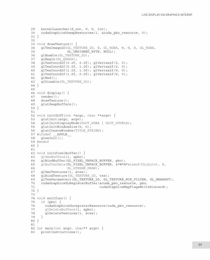
LIVE DISPLAY VIA GRAPHICS INTEROP
59
29 kernelLauncher(d_out, W, H, loc); 30 cudaGraphicsUnmapResources(1, &cuda_pbo_resource, 0); 31 } 32 33 void drawTexture() { 34 glTexImage2D(GL_TEXTURE_2D, 0, GL_RGBA, W, H, 0, GL_RGBA, 35 GL_UNSIGNED_BYTE, NULL); 36 glEnable(GL_TEXTURE_2D); 37 glBegin(GL_QUADS); 38 glTexCoord2f(0.0f, 0.0f); glVertex2f(0, 0); 39 glTexCoord2f(0.0f, 1.0f); glVertex2f(0, H); 40 glTexCoord2f(1.0f, 1.0f); glVertex2f(W, H); 41 glTexCoord2f(1.0f, 0.0f); glVertex2f(W, 0); 42 glEnd(); 43 glDisable(GL_TEXTURE_2D); 44 } 45 46 void display() { 47 render(); 48 drawTexture(); 49 glutSwapBuffers(); 50 } 51 52 void initGLUT(int *argc, char **argv) { 53 glutInit(argc, argv); 54 glutInitDisplayMode(GLUT_RGBA | GLUT_DOUBLE); 55 glutInitWindowSize(W, H); 56 glutCreateWindow(TITLE_STRING); 57 #ifndef __APPLE__ 58 glewInit(); 59 #endif 60 } 61 62 void initPixelBuffer() { 63 glGenBuffers(1, &pbo); 64 glBindBuffer(GL_PIXEL_UNPACK_BUFFER, pbo); 65 glBufferData(GL_PIXEL_UNPACK_BUFFER, 4*W*H*sizeof(GLubyte), 0, 66 GL_STREAM_DRAW); 67 glGenTextures(1, &tex); 68 glBindTexture(GL_TEXTURE_2D, tex); 69 glTexParameteri(GL_TEXTURE_2D, GL_TEXTURE_MIN_FILTER, GL_NEAREST); 70 cudaGraphicsGLRegisterBuffer(&cuda_pbo_resource, pbo, 71 cudaGraphicsMapFlagsWriteDiscard); 72 } 73 74 void exitfunc() { 75 if (pbo) { 76 cudaGraphicsUnregisterResource(cuda_pbo_resource); 77 glDeleteBuffers(1, &pbo); 78 glDeleteTextures(1, &tex); 79 } 80 } 81 82 int main(int argc, char** argv) { 83 printInstructions();

CHAPTER 4 2D GRIDS AND INTERACTIVE GRAPHICS
60
84 initGLUT(&argc, argv); 85 gluOrtho2D(0, W, H, 0); 86 glutKeyboardFunc(keyboard); 87 glutSpecialFunc(handleSpecialKeypress); 88 glutPassiveMotionFunc(mouseMove); 89 glutMotionFunc(mouseDrag); 90 glutDisplayFunc(display); 91 initPixelBuffer(); 92 glutMainLoop(); 93 atexit(exitfunc); 94 return 0; 95 }
This is the brief, high-level overview of what is happening in main.cpp. Lines 1–17 load the header files appropriate for your operating system to access the necessary supporting code. The rest of the explanation should start from the bottom. Lines 82–95 define main(), which does the following things:
• Line 83 prints a few user interface instructions to the command window.
• initGLUT initializes the GLUT library and sets up the specifications for the graphics window, including the display mode (RGBA), the buffering (double), size (W x H), and title.
• gluOrtho2D(0, W, H, 0) establishes the viewing transform (simple orthographic projection).
• Lines 86–89 indicate that keyboard and mouse interactions will be specified by the functions keyboard, handleSpecialKeypress, mouseMove, and mouseDrag (the details of which will be specified in interactions.h).
• glutDisplayFunc(display) says that what is to be shown in the window is determined by the function display(), which is all of three lines long. On lines 47–49, it calls render() to compute new pixel values, drawTexture() to draw the OpenGL texture, and then swaps the display buffers.
• drawTexture() sets up a 2D OpenGL texture image, creates a single quadrangle graphics primitive with texture coordinates (0.0f, 0.0f), (0.0f, 1.0f), (1.0f, 1.0f), and (1.0f, 0.0f); that is, the corners of the unit square, corre-sponding with the pixel coordinates (0, 0), (0, H), (W, H), and (W, 0).
• Double buffering is a common technique for enhancing the efficiency of graphics programs. One buffer provides memory that can be read to “feed” the display, while at the same time, the other buffer provides memory into which the contents of the next frame can be written. Between frames in a graphics sequence, the buffers swap their read/write roles.

LIVE DISPLAY VIA GRAPHICS INTEROP
61
• initPixelBuffer(), not surprisingly, initializes the pixel buffer on lines 62–72. The key for our purposes is the last line which “registers” the OpenGL buffer with CUDA. This operation has some overhead, but it enables low-overhead “mapping” that turns over control of the buffer memory to CUDA to write output and “unmapping” that returns control of the buffer memory to OpenGL for display. Figure 4.2 shows a summary of the interop between CUDA and OpenGL.
• glutMainLoop(), on line 92, is where the real action happens. It repeatedly checks for input and calls for computation of updated images via display that calls render, which does the following:
• Maps the pixel buffer to CUDA and gets a CUDA pointer to the buffer mem-ory so it can serve as the output device array
• Calls the wrapper function kernelLauncher that launches the kernel to compute the pixel values for the updated image
• Unmaps the buffer so OpenGL can display the contents
• When you exit the app, atexit(exitfunc) performs the final clean up by undoing the resource registration and deleting the OpenGL pixel buffer and texture before zero is returned to indicate completion of main().
Figure 4.2 Illustration of alternating access to device memory that is mapped to CUDA to store computational results and unmapped (i.e., returned to OpenGL control) for display of those results

CHAPTER 4 2D GRIDS AND INTERACTIVE GRAPHICS
62
Of all the code in main.cpp, the only thing you need to change when you create your own CUDA/OpenGL interop apps is the render() function, where you will need to update the argument list for kernelLauncher().
Listing 4.6 flashlight/kernel.cu 1 #include "kernel.h" 2 #define TX 32 3 #define TY 32 4 5 __device__ 6 unsigned char clip(int n) { return n > 255 ? 255 : (n < 0 ? 0 : n); } 7 8 __global__ 9 void distanceKernel(uchar4 *d_out, int w, int h, int2 pos) { 10 const int c = blockIdx.x*blockDim.x + threadIdx.x; 11 const int r = blockIdx.y*blockDim.y + threadIdx.y; 12 if ((c >= w) || (r >= h)) return; // Check if within image bounds 13 const int i = c + r*w; // 1D indexing 14 const int dist = sqrtf((c - pos.x)*(c - pos.x) + 15 (r - pos.y)*(r - pos.y)); 16 const unsigned char intensity = clip(255 - dist); 17 d_out[i].x = intensity; 18 d_out[i].y = intensity; 19 d_out[i].z = 0; 20 d_out[i].w = 255; 21 } 22 23 void kernelLauncher(uchar4 *d_out, int w, int h, int2 pos) { 24 const dim3 blockSize(TX, TY); 25 const dim3 gridSize = dim3((w + TX - 1)/TX, (h + TY - 1)/TY); 26 distanceKernel<<<gridSize, blockSize>>>(d_out, w, h, pos); 27 }
The code from kernel.cu in Listing 4.6 should look familiar and require little explanation at this point. The primary change is a wrapper function kernelLauncher() that computes the grid dimensions and launches the kernel. Note that you will not find any mention of a host output array. Computation and display are both handled from the device, and there is no need to transfer data to the host. (Such a transfer of large quantities of image data across the PCIe bus could be time-consuming and greatly inhibit real-time interaction capabilities.) You will also not find a cudaMalloc() to create space for a device array. The render() function in main.cpp declares a pointer d_out that gets its value from cudaGraphicsResourceGetMappedPointer() and provides the CUDA pointer to the memory allocated for the pixel buffer.
The header file associated with the kernel is shown in Listing 4.7. In addition to the include guard and kernel function prototype, kernel.h also contains

LIVE DISPLAY VIA GRAPHICS INTEROP
63
forward declarations for uchar4 and int2 so that the compiler knows of their existence before the CUDA code (which is aware of their definitions) is built or executed.
Listing 4.7 flashlight/kernel.h 1 #ifndef KERNEL_H 2 #define KERNEL_H 3 4 struct uchar4; 5 struct int2; 6 7 void kernelLauncher(uchar4 *d_out, int w, int h, int2 pos); 8 9 #endif
Listing 4.8 flashlight/interactions.h that specifies callback functions controlling interactive behavior of the flashlight app 1 #ifndef INTERACTIONS_H 2 #define INTERACTIONS_H 3 #define W 600 4 #define H 600 5 #define DELTA 5 // pixel increment for arrow keys 6 #define TITLE_STRING "flashlight: distance image display app" 7 int2 loc = {W/2, H/2}; 8 bool dragMode = false; // mouse tracking mode 9 10 void keyboard(unsigned char key, int x, int y) { 11 if (key == 'a') dragMode = !dragMode; // toggle tracking mode 12 if (key == 27) exit(0); 13 glutPostRedisplay(); 14 } 15 16 void mouseMove(int x, int y) { 17 if (dragMode) return; 18 loc.x = x; 19 loc.y = y; 20 glutPostRedisplay(); 21 } 22 23 void mouseDrag(int x, int y) { 24 if (!dragMode) return; 25 loc.x = x; 26 loc.y = y; 27 glutPostRedisplay(); 28 } 29 30 void handleSpecialKeypress(int key, int x, int y) { 31 if (key == GLUT_KEY_LEFT) loc.x -= DELTA; 32 if (key == GLUT_KEY_RIGHT) loc.x += DELTA; 33 if (key == GLUT_KEY_UP) loc.y -= DELTA; 34 if (key == GLUT_KEY_DOWN) loc.y += DELTA;

CHAPTER 4 2D GRIDS AND INTERACTIVE GRAPHICS
64
35 glutPostRedisplay(); 36 } 37 38 void printInstructions() { 39 printf("flashlight interactions\n"); 40 printf("a: toggle mouse tracking mode\n"); 41 printf("arrow keys: move ref location\n"); 42 printf("esc: close graphics window\n"); 43 } 44 45 #endif
The stated goal of the flashlight app is to display an image corresponding to the distance to a reference point that can be moved interactively, and we are now ready to define and implement the interactions. The code for interactions.h shown in Listing 4.8 allows the user to move the reference point (i.e., the center of the flashlight beam) by moving the mouse or pressing the arrow keys. Pressing a toggles between tracking mouse motions and tracking mouse drags (with the mouse button pressed), and the esc key closes the graphics window. Here’s a quick description of what the code does and how those interactions work:
• Lines 3–6 set the image dimensions, the text displayed in the title bar, and how far (in pixels) the reference point moves when an arrow key is pressed.
• Line 7 sets the initial reference location at {W/2, H/2}, the center of the image.
• Line 8 declares a Boolean variable dragMode that is initialized to false. We use dragMode to toggle back and forth between tracking mouse motions and “click-drag” motions.
• Lines 10–14 specify the defined interactions with the keyboard:
• Pressing the a key toggles dragMode to switch the mouse tracking mode.
• The ASCII code 27 corresponds to the Esc key. Pressing Esc closes the graphics window.
• glutPostRedisplay() is called at the end of each callback function telling to compute a new image for display (by calling display() in main.cpp) based on the interactive input.
• Lines 16–21 specify the response to a mouse movement. When dragMode is toggled, return ensures that no action is taken. Otherwise, the components of the reference location are set to be equal to the x and y coordinates of the mouse before computing and displaying an updated image (via glutPostRedisplay()).

LIVE DISPLAY VIA GRAPHICS INTEROP
65
• Lines 23–28 similarly specify the response to a “click-drag.” When dragMode is false, return ensures that no action is taken. Otherwise, the reference location is reset to the last location of the mouse while the mouse was clicked.
• Lines 30–36 specify the response to special keys with defined actions. (Note that standard keyboard interactions are handled based on ASCII key codes [6], so special keys like arrow keys and function keys that do not generate stan-dard ASCII codes need to be handled separately.) The flashlight app is set up so that depressing the arrow keys moves the reference location DELTA pixels in the desired direction.
• The printInstructions() function on lines 38–43 consists of print state-ments that provide user interaction instructions via the console.
While all the code and explanation for the flashlight app took about nine pages, let’s pause to put things in perspective. While we presented numbered listings totaling about 200 lines, if we were less concerned about readability, the entire code could be written in many fewer lines, so there is not a lot of code to digest. Perhaps more importantly, over half of those lines reside in main.cpp, which you should not really need to change at all to create your own apps other than to alter the list of arguments for the kernelLauncher() function or to customize the information displayed in the title bar. If you start with the flashlight app as a template, you should be able to (and are heartily encour-aged to) harness the power of CUDA to create your own apps with interactive graphics by replacing the kernel function with one of your own design and by revising the collection of user interactions implemented in interactions.h.
Finally, the Makefile for building the app in Linux is provided in Listing 4.9.
Listing 4.9 flashlight/Makefile 1 UNAME_S := $(shell uname) 2 3 ifeq ($(UNAME_S), Darwin) 4 LDFLAGS = -Xlinker -framework,OpenGL -Xlinker -framework,GLUT 5 else 6 LDFLAGS += -L/usr/local/cuda/samples/common/lib/linux/x86_64 7 LDFLAGS += -lglut -lGL -lGLU -lGLEW 8 endif 9 10 NVCC = /usr/local/cuda/bin/nvcc 11 NVCC_FLAGS = -g -G -Xcompiler "-Wall -Wno-deprecated-declarations" 12 13 all: main.exe 14

CHAPTER 4 2D GRIDS AND INTERACTIVE GRAPHICS
66
15 main.exe: main.o kernel.o 16 $(NVCC) $^ -o $@ $(LDFLAGS) 17 18 main.o: main.cpp kernel.h interactions.h 19 $(NVCC) $(NVCC_FLAGS) -c $< -o $@ 20 21 kernel.o: kernel.cu kernel.h 22 $(NVCC) $(NVCC_FLAGS) -c $< -o $@
Windows users will need to change one build customization and include two pairs of library files: the OpenGL Utility Toolkit (GLUT) and the OpenGL Extension Wrangler (GLEW). To keep things simple and ensure consistency of the library version, we find it convenient to simply make copies of the library files (which can be found by searching within the CUDA Samples directory for the filenames freeglut.dll, freeglut.lib, glew64.dll, and glew64.lib), save them to the project directory, and then add them to the project with PROJECT ⇒ Add Existing Item.
The build customization is specified using the Project Properties pages: Right-click on flashlight in the Solution Explorer pane, then select Properties ⇒ Configuration Properties ⇒ C/C++ ⇒ General ⇒ Additional Include Directories and edit the list to include the CUDA Samples’ common\inc directory. Its default install location is C:\ProgramData\NVIDIA Corporation\CUDA Samples\v7.5\common\inc.
Application: StabilityTo drive home the idea of using the flashlight app as a template for creat-ing more interesting and useful apps, let’s do exactly that. Here we build on flashlight to create an app that analyzes the stability of a linear oscillator, and then we extend the app to handle general single degree of freedom (1DoF) sys-tems, including the van der Pol oscillator, which has more interesting behavior.
The linear oscillator arises from models of a mechanical mass-spring-damper system, an electrical RLC circuit, and the behavior of just about any 1DoF system in the vicinity of an equilibrium point. The mathematical model consists of a single second-order ordinary differential equation (ODE) that can be written in its simplest form (with suitable choice of time unit) as x″ + 2bx′ + x = 0, where x is the displacement from the equilibrium position, b is the damping constant, and the primes indicate time derivatives. To put things in a handy form for finding solutions, we convert to a system of two first-order ODEs by introducing the

APPLICATION: STABILITY
67
velocity y as a new variable and writing the first-order ODEs that give the rate of change of x and y:
′x = y′y = − x −2by = f x, y , t, …( )
As a bit of foreshadowing, everything we do from here generalizes to a wide variety of 1DoF oscillators by just plugging other expressions in for f(x, y, t, …) on the right-hand side of the y-equation. While we can write analytical solutions for the linear oscillator, here we focus on numerical solutions using finite difference methods that apply to the more general case. Finite difference methods com-pute values at discrete multiples of the time step dt (so we introduce tk = k * dt, xk = x(tk), and yk = y(tk) as the relevant variables) and replace exact derivatives by difference approximations; that is, x′ → (xk+1 – xk) / dt, y′ → (yk+1 – yk) / dt. Here we apply the simplest finite difference approach, the explicit Euler method, by substituting the finite difference expressions for the derivatives and solving for the new values at the end of the time step, xk+1 and yk+1, in terms of the previous values at the beginning of a time step, xk and yk, to obtain:
xk+1
= xk+dt*y
k
yk+1
= yk+dt* −x
k−2by
k( )We can then choose an initial state {xo , yo} and compute the state of the system at successive time steps.
We’ve just described a method for computing a solution (a sequence of states) arising from a single initial state, and the solution method is completely serial: Entries in the sequence of states are computed one after another.
However, stability depends not on the solution for one initial state but on the solutions for all initial states. For a stable equilibrium, all nearby initial states produce solutions that approach (or at least don’t get further from) the equilibrium. Finding a solution that grows away from the equilibrium indicates instability. For more information on dynamics and stability, see [7,8].
It is this collective-behavior aspect that makes stability testing such a good can-didate for parallelization: By launching a computational grid with initial states densely sampling the neighborhood of the equilibrium, we can test the solutions arising from the surrounding initial states. We’ll see that we can compute hun-dreds of thousands of solutions in parallel and, with CUDA/OpenGL interop, see and interact with the results in real time.

CHAPTER 4 2D GRIDS AND INTERACTIVE GRAPHICS
68
In particular, we’ll choose a grid of initial states that regularly sample a rect-angle centered on the equilibrium. We’ll compute the corresponding solutions and assign shading values based on the fractional change in distance, dist_r (for distance ratio) from the equilibrium during the simulation. To display the results, we’ll assign each pixel a red channel value proportional to the distance ratio (and clipped to [0, 255]) and a blue channel value proportional to the inverse distance ratio (and clipped). Initial states producing solutions that are attracted to the equilibrium (and suggest stability) are dominated by blue, while initial states that produce solutions being repelled from the equilibrium are dominated by red, and the attracting/repelling transition is indicated by equal parts of blue and red; that is, purple.
Color Adjustment to Enhance Grayscale ContrastSince it is difficult to see the difference between red (R) and blue (B) when viewing figures converted to grayscale, the figures included here use the green (G) channel to enhance contrast and brightness according to the formula G = 0.3 + (R –B) / 2. Full color images produced by the stability app are available at www.cudaforengineers.com.
The result shown in the graphics window will then consist of the equilibrium (at the intersection of the horizontal x-axis and the vertical y-axis shown using the green channel) on a field of red, blue, or purple pixels. Figure 4.3 previews a result from the stability application with both attracting and repelling regions.
Figure 4.3 Stability map with shading adjusted to show a bright central repelling region and surrounding darker attracting region

APPLICATION: STABILITY
69
We now have a plan for producing a stability image for a single system, but we will also introduce interactions so we can observe how the stability image changes for different parameter values or for different systems.
With the plan for the kernel and the interactions in mind, we are ready to look at the code. As promised, the major changes from the flashlight app involve a new kernel function (and a few supporting functions), as shown in Listing 4.10, and new interactivity specifications, as shown in Listing 4.11.
Listing 4.10 stability/kernel.cu
1 #include "kernel.h" 2 #define TX 32 3 #define TY 32 4 #define LEN 5.f 5 #define TIME_STEP 0.005f 6 #define FINAL_TIME 10.f 7 8 // scale coordinates onto [-LEN, LEN] 9 __device__ 10 float scale(int i, int w) { return 2*LEN*(((1.f*i)/w) - 0.5f); } 11 12 // function for right-hand side of y-equation 13 __device__ 14 float f(float x, float y, float param, float sys) { 15 if (sys == 1) return x - 2*param*y; // negative stiffness 16 if (sys == 2) return -x + param*(1 - x*x)*y; //van der Pol 17 else return -x - 2*param*y; 18 } 19 20 // explicit Euler solver 21 __device__ 22 float2 euler(float x, float y, float dt, float tFinal, 23 float param, float sys) { 24 float dx = 0.f, dy = 0.f; 25 for (float t = 0; t < tFinal; t += dt) { 26 dx = dt*y; 27 dy = dt*f(x, y, param, sys); 28 x += dx; 29 y += dy; 30 } 31 return make_float2(x, y); 32 } 33 34 __device__ 35 unsigned char clip(float x){ return x > 255 ? 255 : (x < 0 ? 0 : x); } 36 37 // kernel function to compute decay and shading 38 __global__ 39 void stabImageKernel(uchar4 *d_out, int w, int h, float p, int s) { 40 const int c = blockIdx.x*blockDim.x + threadIdx.x; 41 const int r = blockIdx.y*blockDim.y + threadIdx.y; 42 if ((c >= w) || (r >= h)) return; // Check if within image bounds

CHAPTER 4 2D GRIDS AND INTERACTIVE GRAPHICS
70
43 const int i = c + r*w; // 1D indexing 44 const float x0 = scale(c, w); 45 const float y0 = scale(r, h); 46 const float dist_0 = sqrt(x0*x0 + y0*y0); 47 const float2 pos = euler(x0, y0, TIME_STEP, FINAL_TIME, p, s); 48 const float dist_f = sqrt(pos.x*pos.x + pos.y*pos.y); 49 // assign colors based on distance from origin 50 const float dist_r = dist_f/dist_0; 51 d_out[i].x = clip(dist_r*255); // red ~ growth 52 d_out[i].y = ((c == w/2) || (r == h/2)) ? 255 : 0; // axes 53 d_out[i].z = clip((1/dist_r)*255); // blue ~ 1/growth 54 d_out[i].w = 255; 55 } 56 57 void kernelLauncher(uchar4 *d_out, int w, int h, float p, int s) { 58 const dim3 blockSize(TX, TY); 59 const dim3 gridSize = dim3((w + TX - 1)/TX, (h + TY - 1)/TY); 60 stabImageKernel<<<gridSize, blockSize>>>(d_out, w, h, p, s); 61 }
Here is a brief description of the code in kernel.cu. Lines 1–6 include kernel.h and define constant values for thread counts, the spatial scale factor, and the time step and time interval for the simulation. Lines 8–35 define new device functions that will be called by the kernel:
• scale() scales the pixel values onto the coordinate range [-LEN, LEN].
• f() gives the rate of change of the velocity. If you are interested in studying other 1DoF oscillators, you can edit this to correspond to your system of interest. In the sample code, three different versions are included corresponding to different values of the variable sys.
• The default version with sys = 0 is the damped linear oscillator discussed above.
• Setting sys = 1 corresponds to a linear oscillator with negative effective stiffness (which may seem odd at first, but that is exactly the case near the inverted position of a pendulum).
• Setting sys = 2 corresponds to a personal favorite, the van der Pol oscil-lator, which has a nonlinear damping term.
• euler() performs the simulation for a given initial state and returns a float2 value corresponding to the location of the trajectory at the end of the simulation interval. (Note that the float2 type allows us to bundle the position and velocity together into a single entity. The alternative approach, passing a pointer to memory allocated to store multiple values as we do to handle larger sets of output from kernel functions, is not needed in this case.)

APPLICATION: STABILITY
71
Lines 34–35 define the same clip() function that we used in the flashlight app, and the definition of the new kernel, stabImageKernel(), starts on line 38. Note that arguments have been added for the damping parameter value, p, and the system specifier, s. The index computation and bounds checking in lines 40–43 is exactly as in distanceKernel() from the flashlight app. On lines 44–45 we introduce {x0, y0} as the scaled float coordinate values (which range from –LEN to LEN) corresponding to the pixel location and compute the initial distance, dist_0, from the equilibrium point at the origin. Line 47 calls euler() to perform the simulation with fixed time increment TIME_STEP over an interval of duration FINAL_TIME and return pos, the state the sim-ulated trajectory has reached at the end of the simulation. Line 50 compares the final distance from the origin and to the initial distance. Lines 51–54 assign shading values based on the distance comparison with blue indicating decay toward equilibrium (a.k.a. a vote in favor of stability) and red indicating growth away from equilibrium (which vetoes other votes for stability). Line 52 uses the green channel to show the horizontal x-axis and the vertical y-axis which intersect at the equilibrium point.
Lines 57–61 define the revised wrapper function kernelLauncher()with the correct list of arguments and name of the kernel to be launched.
Listing 4.11 stability/interactions.h
1 #ifndef INTERACTIONS_H 2 #define INTERACTIONS_H 3 #define W 600 4 #define H 600 5 #define DELTA_P 0.1f 6 #define TITLE_STRING "Stability" 7 int sys = 0; 8 float param = 0.1f; 9 void keyboard(unsigned char key, int x, int y) { 10 if (key == 27) exit(0); 11 if (key == '0') sys = 0; 12 if (key == '1') sys = 1; 13 if (key == '2') sys = 2; 14 glutPostRedisplay(); 15 } 16 17 void handleSpecialKeypress(int key, int x, int y) { 18 if (key == GLUT_KEY_DOWN) param -= DELTA_P; 19 if (key == GLUT_KEY_UP) param += DELTA_P; 20 glutPostRedisplay(); 21 } 22 23 // no mouse interactions implemented for this app 24 void mouseMove(int x, int y) { return; } 25 void mouseDrag(int x, int y) { return; } 26

CHAPTER 4 2D GRIDS AND INTERACTIVE GRAPHICS
72
27 void printInstructions() { 28 printf("Stability visualizer\n"); 29 printf("Use number keys to select system:\n"); 30 printf("\t0: linear oscillator: positive stiffness\n"); 31 printf("\t1: linear oscillator: negative stiffness\n"); 32 printf("\t2: van der Pol oscillator: nonlinear damping\n"); 33 printf("up/down arrow keys adjust parameter value\n\n"); 34 printf("Choose the van der Pol (sys=2)\n"); 35 printf("Keep up arrow key depressed and watch the show.\n"); 36 } 37 38 #endif
The description of the alterations to interactions.h, as shown in Listing 4.11, is also straightforward. To the #define statements that set the width W and height H of the image, we add DELTA_P for the size of parameter value incre-ments. Lines 7–8 initialize variables for the system identifier sys and the parameter value param, which is for adjusting the damping value.
There are a few keyboard interactions: Pressing Esc exits the app; pressing number key 0, 1, or 2 selects the system to simulate; and the up arrow and down arrow keys decrease or increase the damping parameter value by DELTA_P. There are no planned mouse interactions, so mouseMove() and mouseDrag() simply return without doing anything.
Finally, there are a couple details to take care of in other files:
• kernel.h contains the prototype for kernelLauncher(), so the first line of the function definition from kernel.cu should be copied and pasted (with a colon terminator) in place of the old prototype in flashlight/kernel.h.
• A couple small changes are also needed in main.cpp:
• The argument list for the kernelLauncher() call in render() has changed, and that call needs to be changed to match the syntax of the revised kernel.
• render() is also an appropriate place for specifying information to be displayed in the title bar of the graphics window. For example, the sample code displays an application name (“Stability”) followed by the values of param and sys. Listing 4.12 shows the updated version of render() with the title bar information and updated kernel launch call.

APPLICATION: STABILITY
73
Listing 4.12 Updated render() function for stability/main.cpp 1 void render() { 2 uchar4 *d_out = 0; 3 cudaGraphicsMapResources(1, &cuda_pbo_resource, 0); 4 cudaGraphicsResourceGetMappedPointer((void **)&d_out, NULL, 5 cuda_pbo_resource); 6 kernelLauncher(d_out, W, H, param, sys); 7 cudaGraphicsUnmapResources(1, &cuda_pbo_resource, 0); 8 // update contents of the title bar 9 char title[64]; 10 sprintf(title, "Stability: param = %.1f, sys = %d", param, sys); 11 glutSetWindowTitle(title); 12 }
RUNNING THE STABILITY VISUALIZER
Now that we’ve toured the relevant code, it is time to test out the app. In Linux, the Makefile for building this project is the same as the Makefile for the flashlight app that was provided in Listing 4.9. In Visual Studio, the included library files and the project settings are the same as described in flashlight. When you build and run the application, two windows should open: the usual command window showing a brief summary of supported user inputs and a graphics window showing the stability results. The default settings specify the linear oscillator with positive damping, which you can verify from the title bar that displays Stability: param = 0.1, sys = 0, as shown in Figure 4.4(a). Since all solutions of an unforced, damped linear oscillator are attracted toward the equilibrium, the graphics window should show the coordinate axes on a dark field, indicating stability. Next you might test the down arrow key. A single press reduces the damping value from 0.1 to 0.0 (which you should be able to verify in the title bar), and you should see the field changes from dark to moderately bright, as shown in Figure 4.4(b). The linear oscillator with zero damping is neu-trally stable (with sinusoidal oscillations that remain near, but do not approach, the equilibrium). The explicit Euler ODE solver happens to produce small errors that systematically favor repulsion from the origin, but the color scheme cor-rectly indicates that all initial states lead to solutions that roughly maintain their distance from the equilibrium. Another press of the down arrow key changes the damping parameter value to −0.1, and the bright field shown in Figure 4.4(c) legitimately indicates instability.
Now press the 1 key to set sys = 1 corresponding to a system with negative effective stiffness, and increase the damping value. You should now see the axes

CHAPTER 4 2D GRIDS AND INTERACTIVE GRAPHICS
74
on a bright field with a dark sector (and moderately bright transition regions), as shown in Figure 4.5. In this case, some solutions are approaching the equilib-rium, but almost all initial conditions lead to solutions that grow away from the equilibrium, which is unstable.
(a) (b)
(c)
Figure 4.4 Stability visualization for the linear oscillator with different damping parameter values. (a) For param = 0.1, the dark field indicates solutions attracted to a stable equilibrium. (b) For param = 0.0, the moderately bright field indicates neutral stability. (c) For param = -0.1, the bright field indicates solutions repelled from an unstable equilibrium.

APPLICATION: STABILITY
75
Setting the damping param = 0.0 and sys = 2 brings us to the final case in the example, the van der Pol oscillator. With param = 0.0, this system is identical to the undamped linear oscillator, so we again see the equilibrium in a moderately bright field. What happens when you press the up arrow key to make the damping positive? The equilibrium is surrounded by a bright region, so nearby initial states produce solutions that are repelled and the equilibrium is unstable. However, the outer region is dark, so initial states further out produce solutions that are attracted inwards. There is no other equilibrium point to go to, so where do all these solutions end up? It turns out that there is a closed, attracting loop near the shading transition corresponding to a stable period motion or “limit cycle” (Figure 4.6).
Note that the results of this type of numerical stability analysis should be considered as advisory. The ODE solver is approximate, and we only test a few hundred thousand initial states, so it is highly likely but not guaranteed that we did not miss something.
Before we are done, you might want to press and hold the up arrow key and watch the hundreds of thousands of pixels in the stability visualization change in real time. This is something you are not likely to be able to do without the power of parallel computing.
Figure 4.5 Phase plane of a linear oscillator with negative stiffness. A dark sector appears, but the bright field indicates growth away from an unstable equilibrium.

CHAPTER 4 2D GRIDS AND INTERACTIVE GRAPHICS
76
SummaryIn this chapter, we covered the essentials of defining and launching kernels on 2D computational grids. We presented and explained sample code, the flashlight app that takes advantage of CUDA/OpenGL interop to implement real-time graphical display and interaction with the results from 2D compu-tational grids. Finally, we showed how to use flashlight as a template and perform modifications to make it applicable to a real engineering problem, numerical exploration of dynamic stability.
Suggested Projects1. Modify the flashlight app to be a version of the “hotter/colder” game.
Provide an interface for player A to pick a target pixel. Player B then seeks out the target pixel based on the color of the spot, which turns blue (or red) as it is moved farther from (or closer to) the target.
Figure 4.6 Phase plane of the van der Pol oscillator. The bright central region indicates an unstable equilibrium. The dark outer region indicates solutions decaying inwards. These results are consistent with the existence of a stable periodic “limit cycle” trajectory in the moderately bright region.

REFERENCES
77
2. Find another 1DoF system of interest and modify the stability app to study the nature of its equilibrium.
3. The explicit Euler method is perhaps the simplest and least reliable method for numerical solution of ODEs. Enhance the stability app by implement-ing a more sophisticated ODE solver. A Runge-Kutta method would be a good next step into a major field.
4. The van der Pol limit cycle turns out to be nearly circular for param = 0.1. Modify the stability app so the shading depends on the difference between the final distance and a new parameter rad. Implement interactive control of rad, and run the modified app to identify the size of the limit cycle.
References [1] Microsoft Window s Dev Center. “Direct3D,” 2015, https://msdn.microsoft.com/
en-us/library/windows/desktop/hh309466(v=vs.85).aspx.
[2] Mason Woo, Jackie Neider, Tom Davis, and Dave Shreiner, OpenGL Programming Guide: The Official Guide to Learning OpenGL, Version 1.2, Third Edition. (Reading, MA: Addison-Wesley, 1999).
[3] NVIDIA Corporation . “CUDA C Programming Guide,” NVIDIA Developer Zone, CUDA Toolkit Documentation, 2015, http://docs.nvidia.com/cuda/cuda-c-programming-guide/index.html#abstract.
[4] Graham Sellers, Rich ard S. Wright, Jr., and Nicholas Haemel, OpenGL Superbible: Comprehensive Tutorial and Reference, Seventh Edition. (Boston, MA: Addison-Wesley, 2016).
[5] Randi J. Rost et al. , OpenGL Shading Language, Third Edition. (Boston, MA: Addison-Wesley, 2010).
[6] cppreference.com, “A SCII Chart,” 2015, http://en.cppreference.com/w/cpp/language/ascii.
[7] Richard H. Rand. Lectur e Notes on Nonlinear Vibrations, Cornell University eCommons, May 2012, http://hdl.handle.net/1813/28989.
[8] Steven H. Strogatz, Non linear Dynamics and Chaos, Second Edition. (Cambridge, MA: Westview Press, 2014).

This page intentionally left blank

313
Symbols/ (slash), syntax of C language, 248_ (underscore), variable names and, 249# (number or hash sign), syntax of C language, 247() (parentheses), syntax of C language, 247* (asterisk)
as dereference operator, 273syntax of C language, 248
[ ] (brackets), syntax of C language, 247{ } (braces), syntax of C language, 247<<, >> (double angle brackets or chevrons), bit
shift operators, 186<<<, >>> (triple angle brackets or chevrons), in
syntax for parallel computation, 28
Numbers1D grids, computing derivatives on, 81–821DoF, 662D data
locating centroid of state map. See centroid_2d app
solving Laplace’s equation in 2D (heat_2d), 88–92
2D gridsdefining 2D kernel, 52–53dist_2d app, 53–56launching, 50–51moving to 3D grids, 144overview of, 49syntax for 2D kernel launch, 51
3D datacreating vis_3d app, 156generating relocatable device code, 167–170launching 3D computational grids, 144–145listing for dist_3d/kernel.cu, 145listing for vis_3d/device_funcs.cu, 164–167
listing for vis_3d/device_funcs.cuh, 164listing for vis_3d/interactions.h,
159–161listing for vis_3d/kernel.cu, 162–163listing for vis_3d/kernel.h, 161listing for vis_3d/main.cpp, 157–259listing for vis_3d/Makefile, 168–169overview of, 141–143raycasting, 154–156slice visualization of, 149–153viewing and interacting with, 146–149volume rendering, 153
3D gridslaunching computational grids, 144–145steps in, 142uses of, 141
5-point stencil, 91
AAABBs (axis-aligned bounding boxes), in ray-box
intersection testing, 149About CUDA, CUDA resources, 211About This Mac, checking for NVIDIA GPU,
222–223Acceleration, estimating, 17–19Actions/activities, Nsight Visual Studio profiling,
289–290Algebra, using cuSolver and cuBLAS, 201–207ALU (Arithmetic logic unit), in CUDA model for
parallelization, 26Angle brackets or chevrons
bit shift operators, 186in syntax for parallel computation, 28
APIs. See Application programming interfaces (APIs)
Apple computers. See Mac OS X systems
Index

INDEX
314
Application programming interfaces (APIs)creating CUDA apps, 25functions of CUDA Runtime API, 30, 292passing Thrust device vector as argument to
CUDA API function or kernel, 189–190standard graphics, 49
Apps. See also by individual typesbuilding in C programming, 251building in Linux, 258–262building in Windows, 252–258estimating acceleration, 17–19running, 13running serial, 19–22running under Linux systems, 17running under Windows systems, 14–17use in book structure, 4
Argumentspassing by value in C, 246passing CUDA device array as argument to
Thrust function, 189–190passing Thrust device vector as argument to
CUDA API function or kernel, 190typed arguments, 250
Arithmetic logic unit (ALU), in CUDA model for parallelization, 26
Arithmetic operationscompound or augmented assignment, 250in syntax of C language, 248variable names and, 249
ArrayFire library, 207Arrays
coefficient array. See Stencilscomparing serial and parallel computing, 25costs and benefits of standard workflow, 42declarations, 262–263parallelizing dist_v2, 38–42passing CUDA device array as argument to
Thrust function, 189–190producing 2D array of distances from
reference point, 53–56reduction, 121running serial apps, 19–22shared. See Shared arraysunified memory and managed arrays, 43–47using Thrust functions with, 178
Assignmentsarray declarations and, 263
in C programming, 248–250compound or augmented, 250
Asterisk (*)as dereference operator, 273syntax of C language, 248
Asynchronous operations, execution timing and, 282
Atomic functionsavailable in CUDA, 129dealing with race conditions, 128–129specifying value of ATOMIC set, 124use in centroid_2d app, 130
Axis-aligned bounding boxes (AABBs), in ray-box intersection testing, 149
BBasic Linear Algebra Subprograms (BLAS), 201Bit shift operators (<<, >>), 186BLAS (Basic Linear Algebra Subprograms), 201blockDim, 29blockIdx, 29Blocks
about, 26in 3D computational grid, 146choosing execution configuration, 37execution configuration for parallelizing
dist_v2, 41execution configuration of kernel launch, 28launching kernel and, 27organizing threads by, 26sharing information between, 79syntax for 2D kernel launch, 51
Books, CUDA resources, 214–218Bottlenecks, thread, 79Bounding boxes, terminating loops, 155Bounds checking, in 3D computational grid, 146Braces ({ }), syntax of C language, 247Brackets ([ ]), syntax of C language, 247break statements, types of control statements
in C, 267Breakpoints
setting for debugging, 306–308setting when building apps, 256
Bufferingdouble buffering for efficiency of graphics
applications, 60pixel buffers, 61

INDEX
315
Buildsbuilding apps in Linux, 258–262building apps in Windows, 252–258files in build process, 259–260
CC programming
array declarations, 262–263basics, 246–248building apps (create, compile, run, debug),
251building apps in Linux, 258–262building apps in Windows, 252–258characterizations of, 245–246control statements, 263, 267data types, declarations, and assignments,
248–250defining functions, 250–251dist_v1 sample, 267–270dist_v2 sample, 271–275dist_v2 sample with dynamic memory,
275–277foundations for working with CUDA, 3if statements, 265–266invoking NVIDIA C Compiler, 37for loops, 264–265pointer arithmetic, 273samples, 267syntax, 247
C++benefits of unified memory, 44CImg toolkit for, 102–103CUDA development environment based on, 1lambda functions, 183syntax, 176templates, 175
Cache, requirements for minimizing latency, 27Callback functions
defined by interactions.h file, 57keyboard and mouse, 95vis_3d app, 159–161
calloc, creating host array out, 146Case sensitivity
in C language, 249capitalization of variable names, 52
Central processing units (CPUs), GPUs compared with, 26–27
centroid_2d appcentroid_2d/kernel.cu with Thrust,
188–189computing integral properties, 130–131listing for centroid_2d/kernel.cu, 131–133listing for centroid_2d/kernel.h, 135listing for centroid_2d/main.cpp, 135–136listing for centroid_2d/Makefile, 136output image with axes locating centroid,
136–137Chevrons or angle brackets
bit shift operators, 186in syntax for parallel computation, 28
CImg toolkitfor C++, 102–104importing/exporting data from image files, 174
clip(), utility functions of heat2d app, 96clock(), timing methods in C, 280Code
code libraries, 122generating relocatable device code, 167–170libraries. See Librariesplacing Thrust code in .cu file, 177used in book, 8–9
Color, image processing using NPP, 198–199Command-line interface
checking for NVIDIA GPU in Linux, 223console window, 15–17
Compilation, splitting kernel code into multiple files requiring separate compilation, 167–170
Compiled languages, C as, 245Compiler
invoking from IDE, 245invoking NVIDIA C Compiler, 37
Computational grids2D. See 2D grids3D. See 3D grids
Compute capability, 223–224Computed tomography (CT), uses of 3D data
grids, 141Computer graphics, impact on surface
appearance, 156Computing integral properties, 130–131. See also
centroid_2d appConsole window, accessing command-line
interface, 15–17

INDEX
316
Containers, in C++ standard library, 175–176continue statements, types of control
statements in C, 267Control panel, checking for NVIDIA GPU in
Windows, 221–222Control statements, in C
if statements, 265–266for loops, 264–265other options, 267overview of, 263
Conventions, used in book, 8CPUs (central processing units), GPUs compared
with, 26–27CT (computed tomography), uses of 3D data
grids, 141.cu file, placing Thrust code in, 177cuBLAS library, for linear algebra, 201–207CUDA Deep Neural Network (CuDNN) library, 207CUDA ecosystem
books, 214–218CUDA languages and libraries, 217CUDA samples, 217CUDA Zone website, 211–212online courses, 213–214primary web sources, 212–213
CUDA events, 282–284CUDA Random Number Generation (CuRAND)
library, 190–192CUDA Runtime API, 292CUDA Toolkit
about, 1install under Linux, 240install under OS X, 239install under Windows, 230
cudaDeviceSynchronize(), 30cudaFree(), 30cuda-gdb commands
for debugging, 258, 261debugging Linux systems, 305–308
cudaMalloc(), allocating device memory, 36cudaMallocManaged(), allocating memory for
managed arrays, 44CUDA-MEMCHECK tool, error handling with,
308–309cudaMemcpy(), transferring data between host
and device, 44cuDNN (CUDA Deep Neural Network) library, 207
cuRAND (CUDA Random Number Generation) library, 190–192
cuSolver library, for linear algebra, 201–207
DData types
C programming, 248–250CUDA supported, 30for images, 53typed arguments and, 250
dd_1d_global appcomputing derivatives on 1D grid, 81–82implementing, 82listing for dd_1d_global/kernel.cu, 83listing for dd_1d_global/kernel.h, 84listing for dd_1d_global/main.cpp, 82–83listing for dd_1d_global/Makefile, 84
dd_1d_shared app, implementing, 85–88Debugging. See also Error handling; Profiling
building apps in Windows and, 254–258cuSolver and cuBLAS in, 207Debug execution in Visual Studio, 270limitations of Visual Studio or gdb, 38in Linux systems, 305–308viewing thrust vectors in debugger, 190in Windows systems, 298–304
Declarationsarray, 262–263C programming, 248–250
“Deep copy” issues, benefits of unified memory for, 44
Deep Neural Networks, 207#define
specifying input value of function call, 52specifying value of ATOMIC set, 124
Degrees of freedom (DOF)1DOF in stability app, 66–67velocity of 1DOF ocscillators, 70
Densities, of 3D data values, 147Depth, of stack, 144Dereference operator (*), 273Derivatives. See also dd_1d_global app
computing derivatives of a function, 80computing on 1D grid, 81–82implementing dd_1d_global app, 82–85implementing dd_1d_shared app, 85–86solving Laplace’s equation in 2D, 88–92

INDEX
317
Desktop computers, upgrading computing capability of GPU, 226–228
__device__ qualifier, function qualifiers, 29, 45Device
about, 26generating relocatable device code, 167–170lambda, 183passing CUDA device array as argument to
Thrust function, 189–190requirements for changing from serial to
parallel computing, 25–26transferring data between host and device, 44volumetric medical scanners, 141
Devices, 3D data applisting for vis_3d/device_funcs.cu, 164–167listing for vis_3d/device_funcs.cuh, 164
Difference operator, finitecomputing derivatives of a function, 80computing derivatives on 1D grid, 81–82
Differential equations, 66–67Differential equations, equilibrium temperature
distribution, 88–92Digital image processing, uses of 2D grids, 50Digital light projection (DLP), uses of 3D data
grids, 142dim3 variable, CUDA supported vector types, 30Dimension variables, kernel qualifiers, 29Direct numerical simulation (DNS), in fluid
dynamics, 141Direct3D graphics APIs, 49dist_1d app
computing distances, 180for experimental lambda feature compatibility,
183–184listing for dist_1d_thrust/kernel.cu,
180, 184–185listing for dist_1d_thrust/kernel.cu
with device lambda expressions, 183listing for dist_1d_thrust/Makefile, 183
dist_2d appcomputing distances on 2D grid, 54parallel computation of image data based on
distance from reference point in 2D grid, 55–56
producing 2D array of distances from reference point, 53–54
dist_3d app, parallel computation of 3D grid of distances from reference point, 145
dist_v1 appapplying for loop, 19–20C programming sample, 267–270executing dist_v1_cuda, 37–38listing for dist_v1/main.cpp, 267–268parallelizing, 33–37
dist_v1_cuda appexecuting, 37–38parallelizing dist_v1, 33–37
dist_v2 appC programming sample, 271–275creating array of input points, 19dist_v2_cuda/Makefile for building app
with error handling, 295files in, 20–22listing for dist_v1/main.cpp with dynamic
memory management, 276listing for dist_v2/aux_functions.cpp,
273listing for dist_v2/aux_functions.h, 272listing for dist_v2/main.cpp, 271listing for dist_v2/Makefile, 274listing for dist_v2_cuda/kernel.cu for
CPU timing, 280–281listing for dist_v2_cuda/kernel.cu
modified for memory transfer, 283–284modifying for error handling, 294–295parallelizing, 38–42sample with dynamic memory, 275–277
distanceArray() functioncomparing serial and parallel computing, 25parallelizing dist_v2, 41, 44running serial apps, 19–22
Distances2D array of distances from a reference point.
See dist_2d app3D grid of distances from a reference point, 145computing image distance using NPP, 199–200computing using Thrust library, 180–185interactive display of an image based on
distance to a reference point. See flashlight app
parallel distance app. See dist_v2 appserial distance app. See dist_v1 appsigned distance functions, 155
divUp()utility function used with 2D grid, 96utility function used with 3D grid, 144

INDEX
318
DLP (digital light projection), uses of 3D data grids, 142
DNS (direct numerical simulation), in fluid dynamics, 141
do statements, types of control statements in C, 267
Documentation, 212. See also CUDA ecosystemDOF (degrees of freedom)
1DOF in stability app, 66–67velocity of 1DOF ocscillators, 70
Dot productcomputing norms with Thrust built-in
functions, 176–180parallelizing computation of. See
parallel_dot appdotKernel(), dot product kernel, 124dotLauncher(), dot product wrapper function,
124Double buffering, for efficiency of graphics
applications, 60Downloads, CUDA resources, 212Dynamic memory, in serial distance app, 276
EEcosystem. See CUDA ecosystemEducation & Training, CUDA resources, 212–214Element-wise operations, ease of parallelization,
122else clause, using with if statements, 266Embarrassingly parallel, threads with no
interactions between, 122Engineers, value of CUDA for, 3Equilibrium. See also heat_2d app
adding stability app to flashlight app, 67–68
solving Laplace’s equation in 2D, 88–92Error handling. See also Debugging; Profiling
building distance app with error handling, 295with CUDA-MEMCHECK tool, 308–309cuSolver and cuBLAS for, 207modifying dist_v2_cuda/kernel.cu for,
294–295overview of, 292–294
Errors, profiling to test for, 112–117Events, CUDA events, 282–284Executables, locating in bin folder, 14–15Execution configuration
choosing for best performance, 37of kernel launch, 28
for parallelizing dist_v2, 41specifying computational stream number, 87
Execution timingCUDA events and, 282–284overview of, 279–280standard methods in C, 280–282
FFactorization, solving with cuSolver, 202–203Files
in build process, 259–260in dist_v2 app, 20–22in flashlight app, 57importing/exporting data from image files, 174library files, 66makefiles. See Makefiles
Filtering, 79. See also StencilsFinite difference operator
computing derivatives of a function, 80computing derivatives on 1D grid, 81–82
flashlight appadding stability visualizer to. See stability
appexplanation of functionality of flashlight/
interactions.h, 64–65explanation of functionality of flashlight/
main.cpp, 60–61files in, 57interactive display of an image based on
distance to a reference point, 57listing for flashlight/interactions.h,
63–64listing for flashlight/kernel.cu, 62listing for flashlight/kernel.h, 63listing for flashlight/main.cpp, 58–60listing for flashlight/Makefile, 65–66as template, 58, 66
flatten(), utility functions of heat2d app, 97Floating point operations per second (FLOPS), 1Floating-point numbers, associative nature of
floating-point addition in reduction, 130Floating-point units (FPUs), in CUDA model for
parallelization, 26FLOPS (floating point operations per second), 1for loops
control statements in C, 264–265in dist_v1 app, 19–20scale() qualifier, 45syntax of, 264

INDEX
319
FPUs (floating-point units), in CUDA model for parallelization, 26
Function callskernel launch similar to, 28specifying input value of, 52
Function objects (functor), in Thrust transform(), 182
Function qualifiers, 28Functions
of CUDA Runtime API, 30defining in C programming, 250–251overloading, 175parallel functions in NPP, 193passing CUDA device array as argument to
Thrust function, 189–190syntax, 250–251type qualifiers, 28
Functor (function objects), in Thrust transform(), 182
Fusion, 184
Ggdb
cuda-gdb commands, 258, 261, 305–308limitations of debugging tools, 38
GeForce, CUDA-enabled GPUs, 223General purpose GPU (GPGPU), advantages of
parallelism and, 25generate(), estimating Pi using built-in Thrust
functionality, 185–189Getting Started, CUDA resources, 212GLEW (OpenGl Extension Wrangler), 66Global index, referencing global memory, 85Global memory
allocating arrays in device memory, 80–81implementing dd_1d_global app, 82–85profiling, 113slow access speed of, 81transferring data to shared memory, 87
__global__ qualifierdefining 2D kernel, 52kernel qualifiers, 28
GLUT. See OpenGL Utility Toolkit (GLUT)gmake, building apps in Linux, 258goto statements, types of control statements in
C, 267GPGPU (General Purpose GPU), advantages of
parallelism and, 25
Graphical processing units (GPUs)checking for NVIDIA GPU in Linux, 223checking for NVIDIA GPU in OS X, 222–223checking for NVIDIA GPU in Windows,
221–222CPUs compared with, 26–27CUDA-enabled parallel processing, 1–2determining computing capability of, 223–225Kepler GPUs, 133–134memory areas of, 81upgrading computing capability of, 225–228
Graphics, impact on surface appearance, 156Graphics interoperability
adding stability app to flashlight app, 66–69
explanation of functionality of flashlight/interactions.h, 64–65
explanation of functionality of flashlight/main.cpp, 60–61
explanation of functionality of stability/interactions.h, 72–73
explanation of functionality of stability/kernel.cu, 70–71
files in flashlight app sample, 57listing for flashlight/interactions.h,
63–64listing for flashlight/kernel.cu, 62listing for flashlight/kernel.h, 63listing for flashlight/main.cpp, 58–60listing for flashlight/Makefile, 65–66listing for stability/interactions.h,
71–72listing for stability/kernel.cu, 69–70OpenGL graphic package for, 56–57running the stability visualizer app, 73–76using flashlight app as template, 58, 66
gridDim, 29Grids
2D. See 2D grids3D. See 3D gridschoosing execution configuration, 37computational grid in kernel launch, 27computing derivatives on 1D grid, 81–82converting loops to. See Loops, converting to
gridsexecution configuration for parallelizing
dist_v2, 41execution configuration of kernel launch, 28

INDEX
320
HHalo cells
obtaining and storing values of, 87–88use with shared array, 85
Hardware requirements, for changing from serial to parallel computing, 25–26
Hardware setupchecking for NVIDIA GPU in Linux, 223checking for NVIDIA GPU in OS X, 222–223checking for NVIDIA GPU in Windows, 221–222determining computing capability of GPU,
223–225upgrading computing capability of GPU,
225–228Harris, Mark, 133heat_2d app
listing for heat_2d/interactions.h, 95–96listing for heat_2d/kernel.h, 94listing for heat_2d/main.cpp, 92–94solving for equilibrium temperature
distribution in region with specified temperature, 88–89
solving Laplace’s equation in 2D, 89–92Header guard. See Include guardHeterogeneous Parallel Programming, online
courses, 213–214__host__ qualifier, function qualifiers, 28Host
about, 26transferring data between host and device, 44
IIDE (Integrated Development Environment),
invoking compiler from, 245idxclip(), utility functions of heat2d app, 97if statements
control statements in C, 265–266syntax of, 265
Image files, importing/exporting data from, 174Images
data types, 53processing using NPP, 193, 198–201sharpening image edges. See sharpen appsharpening image edges using NPP. See
sharpen_npp appInclude guard, 272Index/indices
for 2D grids, 50–51
for 3D grids, 144array declarations, 263comparing serial and parallel computing, 38in computational grids, 36, 41global and local, 85index variables of kernel, 29for serial loops, 25–27
Inner products, applications of reduction. See parallel_dot app
inner_product(), Thrust built-in functions, 176–180
int type, 41Integer arithmetic, in execution configuration for
parallelizing dist_v2, 41Integral properties, computing, 130–131. See also
centroid_2d appIntegrated Development Environment (IDE),
invoking compiler from, 245Intensities, of pixel values (2D array), 147Interactions, flashlight app
editing callback functions, 58explanation of functionality of flashlight/
interactions.h, 64–65files in flashlight app, 57listing for flashlight/interactions.h,
63–64Interactions, heat_2d app, 95–96Interactions, stability app
explanation of functionality of stability/interactions.h, 72–73
listing for stability/interactions.h, 71–72
Interactions, visualization applisting for vis_3d/interactions.h,
159–161viewing and interacting with 3D data, 146–149
Interactive graphics. See Graphics interoperability
Interop. See Graphics interoperabilityInterpreted languages, compared with compiled,
246Introductory section
benefits of CUDA for engineers, 3–4book structure, 4–6chapter dependencies, 7code used, 8–9conventions used, 8historical context, 10–12

INDEX
321
need-to-know GPU-based parallel computing, 2–3
references, 10–12user’s guide, 9–10what is CUDA, 1–2
Iterators, C++ style, 176
JJacobi iteration
occuring between screen updates, 97reduction and, 122solving Laplace’s equation and, 91
KKepler GPUs, 133–134Kernel
capabilities and limits, 29costs and benefits of standard workflow, 43distanceKernel() qualifier, 45launching, 28mandatory return type is void, 36passing Thrust device vector as argument to
CUDA API function or kernel, 189–190requirements for SIMT implement of
parallelization, 27splitting kernel code into multiple files,
167–170stencil functions, 97–98
Kernel, 1D distance applisting for dist_1d_thrust/kernel.cu,
180, 184listing for dist_1d_thrust/kernel.cu
with device lambda expressions, 183Kernel, 2D distance app
defining 2D kernel, 52–53syntax for 2D kernel launch, 51
Kernel, 3D visualization applisting for vis_3d/kernel.cu, 162–163listing for vis_3d/kernel.h, 161
Kernel, computing derivative on 1D gridkernel.cu, 83kernel.h, 84
Kernel, computing integral propertieslisting for centroid_2d/kernel.cu,
131–133listing for parallel_dot/kernel.h, 135
Kernel, graphics interop appfiles in flashlight app, 57
listing for flashlight/kernel.cu, 62listing for flashlight/kernel.h, 63
Kernel, launch parameters. See Execution configuration
Kernel, parallel dot product applisting for parallel_dot/kernel.cu,
124–125listing for parallel_dot/kernel.h, 125
Kernel, sharpen applisting for sharpen/kernel.cu with global
memory implementation, 105–107listing for sharpen/kernel.cu with input
and output shared memory arrays, 109–112
listing for sharpen/kernel.cu with shared memory implementation, 107–109
listing for sharpen/kernel.h, 104Kernel, stability app
explanation of functionality of stability/kernel.cu, 70–71
listing for stability/kernel.cu, 69–70Kernel, temperature distribution app
kernel functions, 97listing for heat_2d/kernel.cu, 98–100listing for heat_2d/kernel.h, 94
kernelLauncher(), wrapper or launcher functions of heat2d app, 97
Keyboardscallback function, 95callback functions in vis_3d app, 159–161interactions in flashlight app, 60interactions in stability app, 70
Keywords, in C language, 249
LLambda expressions, passing functions and,
183–184Lamberian radiance model, matte appearance
and, 155Languages. See also C programming
compiled, 245CUDA ecosystem, 217Interpreted, 246
Laplace’s equation, solving in 2D (heat_2d), 88–92
Laser Doppler velocimetry (LDV), uses of 3D data grids, 141
Latency, comparing CPUs with GPUs, 27

INDEX
322
Launcher function. See Wrapper functionsLDV (Laser Doppler Velocimetry), uses of 3D data
grids, 141Least-squares problems, solving with cuSolver,
202Libraries
ArrayFire, 207computing distances using built-in Thrust
functionality, 180–185computing norms using built-in Thrust
functionality, 176–180CUDA ecosystem, 217cuDNN, 207cuRAND (CUDA Random Number Generation),
190–192cuSolver and cuBLAS, 201–207customization vs. off-the-shelf approach,
173–175documentation of Thrust library, 175–176estimating Pi using built-in Thrust
functionality, 185–189image processing using NPP, 198–201linking library files, 193–194navigating NPP documentation, 197–198NVIDIA Performance Primitives (NPP), 193passing CUDA device array as argument to
Thrust function, 189–190passing Thrust device vector as argument to
CUDA API function or kernel, 190reduction and, 122Windows system requirements for
flashlight app, 66Linear Algebra Package (LAPACK), 201–202Linear algebra, using cuSolver and cuBLAS,
201–207Linear oscillator. See OscillatorsLinear regression, solving with cuSolver,
203–206Linking. See Libraries, linking library filesLinux software setup
initial test run, 242installing CUDA samples to user directory,
241–242installing CUDA toolkit, 240–241overview of, 240preparing for CUDA installation, 240
Linux systemsbuilding apps using C, 258–262
checking for NVIDIA GPU in Linux, 223converting dist_v1 to executable app, 269debugging in, 305–308invoking NVIDIA C Compiler, 37running CUDA samples under, 17viewing values in managed arrays, 46
Local index, of items in shared array, 85Locals pane, 256Locals window. See Locals paneLoops
for loops. See for loopstermination by exiting bounding box, 155while loops, 155, 267
Loops, converting to gridsexecuting dist_v1_cuda, 37–38overview of, 33parallelizing dist_v1, 33–37simplified workflow, 43–47standard workflow, 42–43
MMac. See OS Xmain()
building apps and, 251in heat_2d app, 91
main.cppdd_1d_global app, 82–83explanation of functionality of flashlight/
main.cpp, 60–61files in flashlight app, 57listing for dist_v1/main.cpp, 267–268listing for dist_v2/main.cpp, 271listing for flashlight/main.cpp, 58–60listing for heat_2d/main.cpp, 92–94listing for parallel_dot/main.cpp, 126,
135–136listing for sharpen_npp/main.cpp,
194–195listing for sharpen/main.cpp, 103–104listing for vis_3d/main.cpp, 157–259
make. See gmakeMakefiles
building Linux apps with, 37for compile/link process, 259–260for dd_1d_global, 84for dist_1d_thrust, 183for dist_v1, 19–20for dist_v1_cuda, 37

INDEX
323
for dist_v2, 22for dist_v2_cuda, 39, 42for flashlight, 65–66for heat_2d, 100–102for parallel_dot, 126–127, 136for sharpen, 105for sharpen_npp, 194for stability, 73for thrustpi, 192
malloc(), allocating host memory, 36Managed arrays
allocating memory for, 44unified memory and, 43–47
Mathematics, foundations for working with CUDA, 3–4
Matlab, ArrayFire and, 207Matrices
reduction and, 122solving linear algebra problems with
cuSolver, 203Memory
developments in memory access, 29dynamic memory management, 276kernel access to device memory not host
memory, 36memory allocation in array declarations, 262“nearer is faster” principle in data storage,
80–81overhead of parallelizing, 42shared memory. See Shared memoryunified memory and managed arrays, 43–47
Monte Carlo estimation, of Pi, 185–189Mouse
callback function, 95specifying interactions for flashlight app,
60
NNamespaces, in resolution of naming conflicts,
176Naming conventions, variables, 52nbody sample
estimating acceleration, 17–18running under Linux systems, 17running under Windows systems, 14–17
“Nearer is faster” principle in data storage, 80–81
Neural networks, 207
Norms, computing using functions in Thrust library, 176–180
Notation, C++, 176Notebook computers, upgrading computing
capability of GPU, 225–226NPP (NVIDIA Performance Primitives) library
image processing using, 198–201linking to NPP files, 193–197navigating NPP documentation, 197–198overview of, 193
Nsightdebugging Linux systems, 305–308debugging Windows systems, 298–304profiling with Nsight Visual Studio, 288–292requirements for running CUDA samples
under Windows systems, 14Number or hash sign (#), syntax of C language,
247nvcc
building apps in Linux, 258handling uchar4 variables, 94invoking NVIDIA C Compiler, 37
NVIDIAchecking for NVIDIA GPU in Linux, 223checking for NVIDIA GPU in OS X, 222–223checking for NVIDIA GPU in Windows, 221–222debugging Linux systems, 305–308debugging Windows systems, 298–304DIGITS, 207invoking NVIDIA C Compiler, 37
NVIDIA Performance Primitives (NPP) libraryimage processing using, 198–201linking to NPP files, 193–197navigating NPP documentation, 197–198overview of, 193
NVIDIA Visual Profiler (NVVP)cross platform visual profiling tool, 284–288profiling to test for errors, 112–117
NVS, CUDA-enabled GPUs, 223Nx acceleration, estimating acceleration, 17–18
OODEs (Ordinary Differential Equations), 66–67Online courses, CUDA resources, 213–214OpenGL Extension Wrangler (GLEW), 66OpenGL graphics package
standard graphics APIs, 49use in graphics interoperability app, 56–57

INDEX
324
OpenGL Utility Toolkit (GLUT)explanation of functionality of flashlight/
main.cpp, 60–61in heat_2d app, 92use in graphics interoperability app, 56–57Windows system requirements for
flashlight app, 66Operating systems
Linux. See Linux systemsMac OS X. See OS X systemsWindows. See Windows systems
Optimus, 225Order of execution, functions for synchronizing
and coordinating, 30Ordinary differential equations (ODEs), 66–67Orthographic projection, as viewing transform, 60Oscillators
adding stability app to flashlight app, 66–69
numerical simulations of dynamics of, 49running stability visualizer, 74–76velocity of 1DOF ocscillators, 70
Overloading, function, 175OS X hardware setup
checking for NVIDIA GPU in OS X, 222–223determining computing capability of GPU,
223–225upgrading computing capability of GPU,
225–226OS X software setup
installing CUDA toolkit, 239–240overview of, 238–239
OS X systems, CUDA gdb deprecated on, 305
PParallel computing
basic tasks, 28–30comparing control of order of execution with
serial computing, 38CUDA model for, 1–2, 25–27hardware setup for. See Hardware setupthreads in, 148
Parallel Forall, CUDA resources, 134, 213Parallel functions, in NPP, 193Parallel patterns, uses of libraries, 174parallel_dot app
associative nature of floating-point addition, 130
atomics as solution to race conditions, 128–129
building and executing, 127–128listing for parallel_dot/kernel.cu,
124–125listing for parallel_dot/kernel.h, 125listing for parallel_dot/main.cpp, 126listing for parallel_dot/Makefile,
126–127parallelizing computation of the dot product of
pair of vectors, 123–124parentheses (( )), syntax of C language, 247Passing by reference, arguments, 246Passing by value, arguments, 246Patterns, uses of parallel patterns, 174PCI, 226–228Performance
choosing execution configuration, 37costs of atomic functions, 129
Piestimating using cuRAND, 190–192estimating using Thrust library, 185–189
Pixels (picture elements)buffers, 61describing pixel values via RGBA, 53–56in digital raster images, 50image processing using NPP, 199locating centroid, 130, 137scaling pixel values, 70
Placeholders, in Thrust transform(), 182Pointer arithmetic, C programming, 273Pointers, use in C, 246pos, as reference position, 146Preprocessors, syntax of C language, 247Primitive data types, in C language, 248printf() statement, support for using from a
kernel, 37–38Profiling. See also Debugging; Error handling
with cuSolver and cuBLAS, 207with Nsight Visual Studio, 288–292with NVIDIA visual profiler, 284–288to test for errors, 112–117
Programming Massively Parallel Processors with CUDA, online courses, 214
Property Pages, Visual Studio, 309–311
QQuadro, CUDA-enabled GPUs, 223

INDEX
325
RRace conditions, resulting in undefined behavior,
128Radar systems, uses of 3D data grids, 141Radius, stencil, 85Random number generation, 190–192Raster images, uses of 2D grids, 50Ray tracing, impact on surface appearance, 156Ray-box intersection tests, 148–149Raycasting
3D data, 154–156overview of, 147sample images of 3D distance field, 143screenshot of vis_3d raycast visualization, 170
rayCastShader(), 153Ray-plane intersection tests, 152Read-modify-write sequence, atomic functions
performing, 128–129reduce(), estimating Pi using built-in Thrust
functionality, 185–189Reduction
associative nature of floating-point addition, 130atomics as solution to race conditions,
128–129computing dot product of pair of vectors,
123–124computing integral properties, 130–131listing for centroid_2d/kernel.cu, 131–133listing for centroid_2d/kernel.h, 135listing for centroid_2d/main.cpp, 135–136listing for centroid_2d/Makefile, 136listing for parallel_dot/kernel.cu,
124–125listing for parallel_dot/kernel.h, 125listing for parallel_dot/main.cpp, 126listing for parallel_dot/Makefile,
126–127output image with axes locating centroid,
136–137overview of, 121threads interacting globally, 121–122
Redundancy, stencil radius and, 85Regression, solving linear regression, 203–206Release folder, accessing CUDA Sample
executables, 15Relocatable device code, splitting kernel code
into multiple files, 167–170render(), in heat_2d app, 91
ResetKernel(), in heat2d app, 97resetTemperature(), in heat2d app, 97Resources. See CUDA ecosystemRGB (red, green, blue) color model, image
processing using NPP, 198–199RGBA
describing pixel values, 53–56initializing GLUT library and, 60
Rootfinding, locating point where function takes on given value, 155
Runtime APIerror handling and, 292functions of CUDA Runtime API, 30
SSamples, CUDA resources, 217Scalability, of SIMT approach, 26Scalar products, applications of reduction. See
parallel_dot appScoping, defining functions, 250Seismic exploration, uses of 3D data grids, 141Separate compilation. See Relocatable device
codeSerial computing
comparing control of order of execution with parallel computing, 38
comparing serial and parallel computing, 25running serial apps, 19–22
Serialization, costs of atomic functions, 129Shading functions
rayCastShader(), 153sliceShader(), 151–153volumeRenderShader(), 153
Shared arraysdeclaring, 86, 133index of items in, 85setting size of, 87
Shared memorybridging gap between memory access and
speed, 81computing derivatives on 1D grid, 81–82declaring shared array, 133declaring threads as shared, 123image sharpening app, 103implementing dd_1d_global app, 82–85implementing dd_1d_shared app, 85profiling, 114sharing information between blocks, 79

INDEX
326
Sharing models, impact on surface appearance, 156
sharpen applisting for sharpen/kernel.cu with global
memory implementation, 105–107listing for sharpen/kernel.cu with input
and output shared memory arrays, 109–112
listing for sharpen/kernel.cu with shared memory implementation, 107–109
listing for sharpen/kernel.h, 104listing for sharpen/main.cpp, 103–104listing for sharpen/Makefile, 105profiling to test for errors, 112–117sharpening image edges, 102–103
sharpen_npp applisting for sharpen_npp/main.cpp,
194–195listing for sharpen_npp/Makefile, 194reimplementation of sharpen app using NPP,
194Signal processing, NPP functions for, 193Signed distance function, 155Single instruction multiple thread (SIMT)
limits on thread accessibility, 123model of parallelization, 26
Slash (/), syntax of C language, 248sliceShader() function, 151–153Slicing
overview of, 147sample images of 3D distance field, 143screenshot of vis_3d slicing, 169slice visualization of 3D data, 149–153
SMs. See Streaming multiprocessors (SMs)Software
requirements for changing from serial to parallel computing, 25
requirements for SIMT implement of parallelization, 27
setup for Mac OS X. See Mac OS X software setup
setup for Windows OSs. See Windows software setup
stability appexplanation of functionality of stability/
interactions.h, 72–73explanation of functionality of stability/
kernel.cu, 70–71
listing for stability/interactions.h, 71–72
listing for stability/kernel.cu, 69–70running the stability visualizer app, 73–76stabilizing visualization app, 69–70
Stack (or stratum), integer variable used in indexing, 144
Stack overflow error, 146StackOverflow, CUDA resources, 213Standard Template Library (STL), Thrust based
on, 175–176State map, locating centroid on. See
centroid_2d appSteady-state temperature distribution. See also
heat_2d appoverview of, 91reduction and, 122
Stencils5-point stencil, 91computing derivatives on 1D grid, 81–82implementing dd_1d_global app, 82–85implementing dd_1d_shared app, 85–88kernel functions, 97–98listing for heat_2d/interactions.h, 95–96listing for heat_2d/kernel.cu, 98–100listing for heat_2d/kernel.h, 94listing for heat_2d/main.cpp, 92–94listing for heat_2d/Makefile, 100–102overview of, 79radius, 85sharpening image edges. See sharpen appsolving Laplace’s equation in 2D (heat_2d),
88–92thread interdependence and, 80–81
STL (Standard Template Library), Thrust based on, 175–176
Stratum (or stack), integer variable used in indexing, 144
Streaming multiprocessors (SMs)choosing execution configuration, 37in CUDA model for parallelization, 26–27thread interdependences and, 80
Streams, specifying computational stream number, 87
Synchronous operationserror handling and, 292execution timing and, 282
__syncthreads(), synchronization of threads, 88

INDEX
327
TTEGRA/Jetson, CUDA-enabled GPUs, 223Temperature, equilibrium temperature
distribution. See heat_2d appTemperature distribution, equilibrium. See
heat_2d apptempKernel(), kernel functions of heat2d app,
97Templates
C++ template library, 175–176flashlight app as, 58, 66
Tesla, CUDA-enabled GPUs, 223Tests, for errors, 112–117. See also ProfilingText editors, for Linux and OS X, 258Threadblocks, launching kernel and, 27threadIdx, 29Thread
about, 26bottlenecks, 79breaking tasks into subtasks, 26choosing execution configuration, 37debugging Linux systems, 307execution configuration for parallelizing
dist_v2, 41execution configuration of kernel launch, 28interacting globally, 121–122interdependence, 80–81launching kernel and, 27limits on accessibility, 123in parallel computing, 148synchronization of, 88
threads per block (TPB), defining constant values in parallel_dot app, 124
Thrust librarycomputing distances, 180–185computing norms, 176–180documentation of, 175–176estimating Pi, 185–189passing CUDA device array as argument to
Thrust function, 189–190passing Thrust device vector as argument to
CUDA API function or kernel, 190using with arrays, 178
thrustpi app, 186–188, 190–192<time.h>, timing methods in C, 280Timing. See Execution timingTools, CUDA resources, 212
TPB (threads per block), defining constant values in parallel_dot app, 124
Traces, Nsight Visual Studio profiling, 289–290Training, CUDA resources, 212–214transform()
computing distances using built-in Thrust functionality, 180–185
estimating Pi using built-in Thrust functionality, 185–189
Triggers, Nsight Visual Studio profiling, 289–290Type qualifiers, functions, 28Typed arguments, defining functions in C, 250Typed languages, C as, 246
Uuchar4 variables, nvcc handling of, 94Udacity CS344:Intro to Parallel Programming,
online courses, 213uint3 variable, CUDA supported vector types, 30Underscore ( _), variable names and, 249Unified memory
creating a simplified workflow, 43–47notes regarding use of, 44
Unsharp masks, 102–103Upgrades, computing capability of GPU, 225–228
Vvan der Pol oscillator
adding stability app to flashlight app, 66
phase plane of, 76Variables
capitalization of variable names, 52declaring and naming in C, 248–249
Vectorscontainer in C++ standard library, 175–176CUDA supported data types, 30parallelizing computation of the dot product of
pair of. See parallel_dot apppassing Thrust device vector as argument to
CUDA API function or kernel, 189–190using Thrust functions with arrays instead of
vectors, 178viewing thrust vectors in debugger, 190
Video processingNPP functions for, 193uses of 3D data grids, 142

INDEX
328
vis_3d appcreating, 156listing for vis_3d/device_funcs.cu, 164–167listing for vis_3d/device_funcs.cuh, 164listing for vis_3d/interactions.h, 159–161listing for vis_3d/kernel.cu, 162–163listing for vis_3d/kernel.h, 161listing for vis_3d/main.cpp, 157–259listing for vis_3d/Makefile, 168–169viewing and interacting with 3D data, 146–149
Visual Profiler. See NVIDIA Visual Profiler (NVVP)Visual Studio
building apps in Windows, 252–258Debug execution, 270limitations of debugging tools, 38messages and warnings, 275Property Pages, 309–311
Visual Studio Community 2013, 14Visualization of data
slice visualization of, 149–153viewing and interacting with 3D data. See
vis_3d appvoid, mandatory return type for kernel, 36Volume elements (voxels)
length scale set by voxel spacing, 155moving from 2D grids to 3D grids, 144
Volume rendering3D data, 153overview of, 147sample images of 3D distance field, 143screenshot of vis_3d volume rendering, 170
volumeRenderShader(), 153Voxels (volume elements)
length scale set by voxel spacing, 155moving from 2D grids to 3D grids, 144
WWarps, dividing blocks into, 26–27Watch window, 277Web resources
CUDA Zone website, 211–212primary web sources, 212–213
while loopstermination by exiting bounding box, 155types of control statements in C, 267
White spaces, in C language, 249Wikipedia, CUDA resources, 213Windows hardware setup
checking for NVIDIA GPU in Windows, 221–222determining computing capability of GPU,
223–225Windows software setup
creating restore point, 230initial test run, 235–238installing CUDA toolkit, 230–234installing IDE, 230steps in, 229
Windows systemsbuilding apps using C, 252–258converting dist_v1 to executable app, 269debugging in, 298–304invoking NVIDIA C Compiler, 37running CUDA samples under, 14–17viewing thrust vectors in debugger, 190viewing values in managed arrays, 46–47
Workflowanalyzing costs and benefits of CUDA, 42–43unified memory simplifying, 43–47
Wrapper functionsabout, 41in vis_3d app, 161