Pragmatic Trading

Use of Weapons

Revision 1.2

Kevin D. Morgan

Published by Kevin D. Morgan

Copyright 2020, Kevin D. Morgan

Table of Contents

Use of Weapons .......................................................................... 1

Introduction ................................................................................. 2

Basic Features of Trading Weapons ............................................ 4

Direct Purchase ....................................................................... 4

Buying Options ........................................................................ 7

Selling Options ....................................................................... 14

Selling Vertical Spreads ......................................................... 17

The Psychology of Selling Vertical Spreads vs. Direct Purchase

.............................................................................................. 25

Adding EV Through Market Structure ........................................ 26

Trade Benefits of Selling Out of the Money Premium ................. 34

Spreading Close to the Money................................................... 34

Spreading In the Money ............................................................ 37

Bracketing Price with Sold Iron Condors .................................... 39

General Trade Portfolio Considerations ..................................... 43

Earnings Considerations............................................................ 45

Conclusions ............................................................................... 45

Introduction This book presents a methodology for leveraging an edge in the market achieved through analysis to achieve a consistent generation of profits with low variance and high efficiency. The methodology is based on the selling of option spreads in specific markets, at specific strikes and expiration dates, with appropriate risk management and profit management techniques. The objective of this book is to thoroughly document the pros and cons of this approach (particularly relative to outright purchase or shorting of an instrument), the underlying mathematical logic, and the specifics of its implementation. This book presents the final 5% you need to know to consistently extract profits from the stock market. The first 95% is presented in my book "Pragmatic Trading: Professional Planning, Modern Methods", which comprehensively addresses how to achieve trade edge through market analysis and formal trading planning and execution. The presumption throughout that book, for simplicity, is the use of direct purchase (or sale) of the stock and ETF instruments and trading for profits based on price movement.

In this volume, I turn to the subject of "use of weapons". Once we have an edge through our analysis, we are still faced with an extraordinary breadth of choice in how to formulate market bets. This breadth is enabled by the availability of stock or ETF options contracts, which can be combined to form a large number of different bet types on a market. Of particular interest for us is the general structure of betting on "half the chart", that is, a bet that pays +$X if the underlying instrument is above or below a particular price level $P at a particular point in time (the expiry date of the option), and loses -$Y at expiry otherwise. Such bets can be placed just about any time, with the above/below line just about anywhere, with varying implications for profit and loss levels, and maximum risk. Using this type of bet structure, particularly when coupled with effective low-cost de-risking exit strategies, will be shown to combine synergistically to give us extraordinary total edge (total +EV) in our market operations, with the important additional features of low variance and high-profit generation efficiency (percentage profit over time). This book will presume an understanding of the basic concepts of stock options; if not, I refer you to McMillan's books on options, and other option fundamental text. In particular, while the fundamentals are covered in this book, it is best if you already have a firm understanding of the basic concept and mechanics of "selling an option spread", or use of "credit spreads". A credit spread means selling a higher-priced option and buying a lower-priced option (of the same type, calls for bearish bets, and puts for bullish bets) with the same expiration date, with the goal that both expire worthlessly and your total profit is the income from the overall transaction. While we call the transaction "selling a spread", the actual transaction involves both selling and buying

options, generating net income, which if both options expire worthlessly is our profit.

Basic Features of Trading Weapons

Direct Purchase

After spending lots of time and effort learning how to analyze and identify excellent trading edge situations in the market, on what basis do we select our trading weapons? Note: I often use "stalking" as a metaphor for waiting for a setup and taking a trade on a trigger; it is analogous to the stalking of prey in the wild, the observation of the game, and then the final approach and shot, which naturally leads to the "choice of weapon" as a metaphor for deciding exactly how to place a bet given a setup and trigger.) Proper selection of alternative bet types in the market starts with a deep understanding of the relative pros and cons of each. Let's start with the simple purchase (or sale for shorts) of the instrument (the stock or ETF).

This is a profit and loss curve for the direct purchase of a tradable instrument, in this case, the stock AAPL. The x-axis is the price of the instrument. The y-axis is the profit or loss level. With direct purchase, our result is independent of time, so there is only one profit/loss curve here (a straight line at a particular slope). With direct purchase, we experience "instant results" in a linear manner with the change in the price of the instrument. We experience our full potential profit or loss (relative to the current price) should we choose at any time to exit the trade; there is no element of accrual of profits, nor mounting losses, over time (without price movement) with direct purchase. There is no "profit at date X" line on this chart, as there is on options charts because our profit/loss amount is time-invariant. Thus the single line represents our profit or loss amount at any price at any time, now or in the future, based solely on the price of the instrument at the present moment. The second attribute of direct purchase is that we have unlimited profits, coupled with unlimited loss (all of the capital exposed). Our gains and/or losses are linear with the change of price of the instrument, to infinity as well as to zero. Thus, we have both a high-risk element (all our money is exposed to potential total loss) and a high reward element (if the price suddenly goes up 5x, the value of our asset goes up linearly by 500%, and we stand to make 400% profit). This feature is a significant value. However, with options, this value can be traded off for other values (we cap our wins to get other benefits). The third key attribute of direct purchase is that we must always place our "zero price" (the price of the instrument at which we have zero profit and zero loss if we exit) at the current price of the instrument. There is no way to shift the zero line (at the cost for example of changing our win/loss sizes). This is a tremendous

limitation. In a sense, we are only allowed to play 50%-50% odds bets (under the assumption that price action is random). A subtle but critically important fourth attribute of direct purchase is that our time horizon for profit or loss is unlimited. That is, to achieve any particular target profit level or loss (stop and exit) level, we may have to wait "forever". Time in these trades is bounded only by our willingness to remain in the trade; intrinsically the trade has no time boundary. Direct purchase bets are fundamentally 50%/50% odd bets. That is, ignoring any edge one has through market analysis, and ignoring any edge one may have because of long term market bias, any direct purchase bets that the market will be up (or be down through shorting) after any defined fixed period is a 50% proposition. And ignoring costs (pragmatically a horrible idea but for the sake of this analysis is okay) the expected value (EV) of every direct purchase bet using a fixed time-based exit is zero; it is essentially a coin flip result. This point bears restating: our starting point odds are only 50% of winning in every direct purchase bet. Trade management practices don't fundamentally change this (or at the best change it very little). And there is no means with direct purchase wherein we can structure (as an example) a zero EV bet that has a 75% chance of profiting but pays at a win-loss ratio of 1-3 (making it effectively a 50%-50% bet). To have higher odds of winning with direct purchase, we must use our analytical skills to get an edge that shifts our trade odds from 50% to something higher. Here's the summary of attributes for the trading method of direct purchase:

Instant linear profit/loss with the price movement of the instrument.

Unlimited potential profit and potential for a total loss.

Always a baseline 50%-50% bet (i.e., odds of being a winner vs. a loser at any fixed time in the future).

Unlimited time (no guarantee of "ever") to achieve any given target level of profit.

Buying Options

Stock and ETF options are extremely flexible financial instruments. They can be purchased, they can be sold, and they can be purchased and/or sold in various combinations. A call option gives the owner the right to buy from the seller the underlying instrument (100 shares per option contract) at the strike price of the option, up until the expiry date of the option. A put option gives the owner the right to sell to the seller of the option the underlying instrument (100 shares per option contract) at the strike price of the option, up until the expiry date of the option. The reverse contract terms apply to the seller of calls and puts: a seller of calls must be able to deliver 100 shares of the underlying in return for payment at the strike price, should the owner ever decide to execute the option (this event is often termed "called away"). A seller of puts must be able to buy 100 shares of the underlying and pay the owner of the option the strike price for them (this even is often termed "assigned"). Getting sold call or put options exercised by the owner is something we strongly want to avoid. The one exception to this is when we are interested in buying an instrument outright but instead sell naked put options, with the overt intent of taking ownership of the stock (at a discount due to the sale of the put options) if as expiry approaches the put options are in the money (in which case, the owner will exercise and assign the stock to you).

Options prices have two components: intrinsic value, and an extrinsic, or premium value. The intrinsic value is the difference between the price of the underlying instrument at this moment and the strike price of the option. If the strike is out of the money (higher than the current price for calls, and less than the current price for puts), then the intrinsic value is zero. The premium value is the cash value associated with the rights the option provides the owner: namely, the right to buy (calls) or sell (puts) 100 shares (per option) of the underlying on or before the expiry date at the strike price of the option. The more time remaining on the option, the more such value the option has, and the larger the premium. As time moves forward and the remaining time left on the option reduces, the premium amount decays. It decays in an accelerating curve with a very substantial collapse in the last few days, and even faster collapse in the last few hours and then minutes of the life of the option. (Note: "premium" is used two different ways in the options word. Some define premium as the total price of the option, while others define premium as strictly the extrinsic component of the total price of the option. Here is the definition of "premium" from optionstrading.org:

Premium: A term that can be used to describe the whole price of an option or the extrinsic value of an option.

In this text, "premium" refers strictly to the extrinsic value of options.) In addition to the premium value being dictated by time, the premium is also dictated by the price of the underlying, a manner somewhat analogous to how and why intrinsic value varies with the changing price of the underlying. This attribute is obvious in the price of options for a common expiry across strike prices

moving deeper and deeper out of the money. The option prices reflect premium only, with the same amount of time left on all the options, but the options prices steadily decay as the strike price moves further away from the current price. Premium price implicitly reflects the odds of the option ending up "in the money" (having some intrinsic value at expiration). The further price is from the strike price, the lower the odds of this happening, and hence, the lower the premium, which for options out of the money had no intrinsic value, so all of the option pricing is the premium value (time value associated with the rights of the option). Hence, the premium of every stock option is specified by three components: the amount of time remaining (more time, more value, and more premium), the odds of the option ending up "in the money" (having an intrinsic value at expiration), and the price of the underlying instrument. Why does the price of the underlying instrument impact the premium? Because every option is for 100 shares of the instrument. If the instrument is $10/share, you are controlling $1000 worth of assets, whereas if the instrument is $100/share, you are controlling $10,000 worth of assets. The time rights of a contract for $10,000 worth of goods is worth 10x the value of a contract for $1000 worth of goods. What determines the odds of the option ending up "in the money". Two options on different underlying instruments that have an identical price with the same expiry date and both strikes 5% out of the money may have very different prices. Why? Because one instrument has demonstrated very low historical price volatility on a percentage basis recently, while the other has very high historical price volatility. The higher the price volatility of the

underlying, the higher the chances of the price being in the money at expiry, the higher the premium. Another term of importance is implied volatility, ofter referred to as IV. The concept of IV is that the extrinsic value of an option is a forward-looking assessment of volatility of the price of the underlying, considering all possible factors. While IV can be computed using those factors, pragmatically, IV is expressed as the extrinsic value of the option. It's critical to be aware that the extrinsic price component of an option is impacted by factors beyond just the drivers of historical volatility and time remaining. Other reasons for expectations on increased volatility in the price of the underlying arise, and drive changes in the extrinsic. The most common and recurring reason is quarterly earnings for individual stocks. Earnings announcements release a flood of information about the state of the company and often drives very large and rapid change in the price of the stock. Hence, as an earning announcement approaches, there will typically be a rise (sometimes quite significant) in the extrinsic price component of the total price of the options. This rise on a relative basis will be more pronounced in the shorter-dated options. Here is a daily chart of NFLX, showing the implied volatility as represented by the extrinsic price. Quarterly earnings dates are marked, you can see the clear and regular rise and fall of IV through each earnings date. This is a significant factor to be considered when trading with options, as will be covered below in the various option trading strategies.

We can and do use the pricing of options to inform us about odds. The option price reflects a bet with zero expected value. What that price needs to be to give that result is dependent on the time remaining until expiry, the strike price of the option vs. the current market price of the instrument, and the expectations of volatility between the present moment and the expiration date. If price approaches the option strike price, the odds of expiring in the money increase, and the price of the option increases. Note that this increase is NOT linear like it is with the change of intrinsic value with price. The rate of change in odds is higher when the price of the instrument and the strike prices are close, and lower when they are far apart (for the same absolute change in price). What happens to premium as an option moves into and farther into the money? The odds of the option ending in the money goes up, so the extrinsic (as well as the intrinsic) increases. However, while the intrinsic component of options price moves up linearly with the instrument price moving the option further into the money, the extrinsic component of the options price increases at a slowly decreasing rate as the same occurs. This is because of

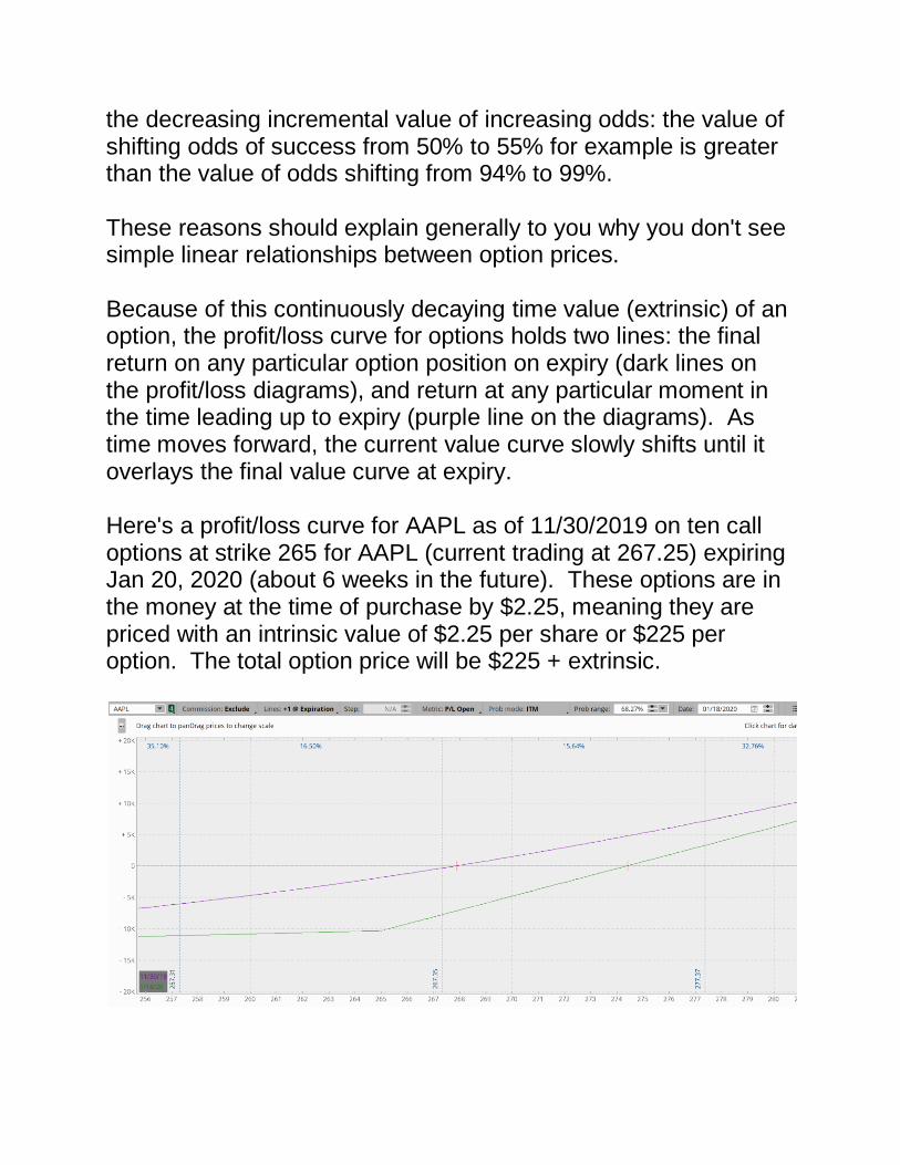
the decreasing incremental value of increasing odds: the value of shifting odds of success from 50% to 55% for example is greater than the value of odds shifting from 94% to 99%. These reasons should explain generally to you why you don't see simple linear relationships between option prices. Because of this continuously decaying time value (extrinsic) of an option, the profit/loss curve for options holds two lines: the final return on any particular option position on expiry (dark lines on the profit/loss diagrams), and return at any particular moment in the time leading up to expiry (purple line on the diagrams). As time moves forward, the current value curve slowly shifts until it overlays the final value curve at expiry. Here's a profit/loss curve for AAPL as of 11/30/2019 on ten call options at strike 265 for AAPL (current trading at 267.25) expiring Jan 20, 2020 (about 6 weeks in the future). These options are in the money at the time of purchase by $2.25, meaning they are priced with an intrinsic value of $2.25 per share or $225 per option. The total option price will be $225 + extrinsic.

The final value of the options is always the intrinsic value alone, and if the intrinsic value is zero (price is below the strike at expiry for call options and above the strike at expiry for put options), the options expire worthlessly. The seller keeps all the money received for the sale, and the buyer losses all the money spent on the purchase of the option. Note how in the current value curve, the steepest rate of change (the first derivative) of the curve is right around the strike price. The further reaches of the curve "flattens out" and becomes a more linear curve. The explanations above of option pricing are the reasons for this: the extrinsic price component that reflects "odds" is not linear across price, and changes most rapidly around the strike price. When we are buyers of options, we bear the cost of the decaying extrinsic. We are in a race against time, to have the underlying change in price (in our profit direction) faster than time extrinsic decay to create an incremental total market value of the option vs. what we originally paid. This is visible in the AAPL call option diagram as the position of the red line crossing the zero profit/loss level on the y-axis (red tick), and the final zero price at option expiry (the red tick on the green line). As the call option buyer, the underlying instrument price must get from "here to there" faster than the decaying (time-based) extrinsic and hence the total value of the option (the purple curve descending to the green curve over time, matching it exactly at option expiry), or we will never even have the opportunity to exit at any time with any profit at all. Again, as time passes extrinsic decays at a faster and faster rate, and more total price movement in our direction over the same amount of time is required to "keep up" much less get highly profitable.

Selling Options

Now let's look at the inverse position. Here's the profit/loss curve for selling (not buying) a single put option in AAPL. This option is slightly out of the money put option at strike 265 for January 20, 2020, as of 11/30/2019 when the price of AAPL is 267.25. This curve shows the profit/loss level down to AAPL going to zero in price.

What happens if AAPL goes to zero? As the seller of a single put option in AAPL, we are obligated to buy 100 shares from the owner of the put at the strike price. So we spend $26500 to buy 100 shares of AAPL, and we can sell them for $0. (Note: we also have the money from the sale of the put option, about $870, so our net loss is "only" $25630). We have lost almost the same amount as if we had bought and held 100 shares of AAPL at the strike price of 265 until the price of AAPL stock reached zero. It's critical to understand this aspect of selling puts. As a put seller, we are financially responsible for the ownership of 100

shares of the underlying. For this reason, our trading margin will be reduced by the amount of the strike price of the option times 100 per option sold (roughly). It's no different than the impact on our buying power when we buy 100 shares of the underlying. This buying power impact is important because when we know how to get a significant edge in the market and conditions are ripe, we want to get all of our money working for us as efficiently as possible. Utilizing all of the buying power implied by the risk side of the option curve above to gain a comparatively very small profit is inefficient. Additionally, while we are likely in theory to exit well before a stock like AAPL moves down in price so substantially, that's not always possible (price often moves "overnight" and we can't act until the day session market opens). Simply put, the open risk of selling naked puts is extraordinarily high. Here's a view of the profit/loss curve for the same sold put in AAPL, focused on the price range that is likely over the life of the option (6 weeks).

Note the probability "slice" lines (vertical dashed lines with probability figures). One is placed at the expiration curve (green

line) zero profit/loss level (AAPL at 261.30). The 58.42% to the upper right tells us that based on the price of the option (which in turn reflects the price volatility of the AAPL stock), there is a 58.42% chance that the price will be in this zone of profit at the expiry date. Similarly, the sum of the two probabilities to the right tells us the probability of having a loss at expiry: 41.58%. The probability slice at 252.60 is positioned where the loss amount at expiry is the same as the max win size. Our probability of suffering a loss larger than our maximum possible win is about 28%. Underlying these probabilities are our win and loss sizes, on average, per these probabilities of a win or loss occurring. The sum overall is always zero, if the options are priced accurately (per Black Scholes and similar option pricing models). And arbitrage of the options assures that any lack of balance (a positive EV for selling or buying the option, and a negative EV for the opposite) will be corrected quickly by traders looking to take advantage of such an edge. For the AAPL sold put option above there is a 58.42% of winning, which implies an average win size (as a percentage) vs. average losing trade size. The equation is formed by the logic that the average win size x times the win frequency (0.5842 of the time) plus the average loss size y times the loss frequency (which is 1-win frequency, or 0.4158) is zero. Hence:

0.5842x + 0.4148y = 0

0.4842x = -0.4148y

x = -0.71y

x = -y / 1.4

1.41x = -y

Ergo, the average win size to loss size is 1.41/1. These are the probabilities associated with buying this call option in AAPL from the perspective of a random market with the volatility levels experience in AAPL stock in the recent past. There is zero assumption in these probabilities and computations of average win and loss sizes about any significance of AAPL's trend, or otherwise about future expectations. Random price movement at the recent levels of volatility is the underlying assumption. Let's review the generic attributes of selling puts, and compare those to direct purchase of the underlying instrument:

Potential profit varies with changing price but not less than linearly.

Profit (or reduction of loss) increases (accrues) over time.

The maximum risk is the full value of the underlying (similar to direct purchase).

The maximum profit is CAPPED.

Odds (assuming random price movement) are ADJUSTABLE based on the selection of puts (strike and expiry date).

Trade time is limited; there is a fixed time horizon for exiting.

Selling Vertical Spreads

To address the problem of extremely large (relative to the maximum win size) maximum loss, and also quite importantly, the impact to our margin (reduction of buying power) of selling puts, we now move to sell put vertical spreads. A vertical option spread is a purchase and sale of two options of similar type (puts or calls), for the same expiration date, with

different strikes. Buying a vertical spread refers to buying more expensive options while selling less expensive options for a net debit. For calls, buying a vertical spread means buying a call option at a lower strike and selling a call at the same expiry at a higher strike. For puts, buying a vertical spread means buying a call option at a higher strike and selling a put at the same expiry at a lower strike. Selling a spread refers to selling more expensive options and buying less expensive options for the same expiry for a net credit. For calls, selling a vertical spread means selling a call at a lower strike price and buying a call at the same expiry at a higher strike. For puts, selling a vertical spread means buying a put at a higher strike price and buying a put at the same expiry at a lower strike price. Buying a call spread (a debit spread) is a bullish play while buying a put spread (also a debit spread) is a bearish play. Selling a call spread (a credit spread) is a bearish play while selling a put spread (also a credit spread) is a bullish play. When selling spreads, the objective is rather simple: we want the price at the expiration of the option contract to be in the price area that makes both the bought and sold options worthless, allowing us to keep the full net proceeds of the transaction. We lose all the money on the purchased option, and make all the money on the sold option, for a net profit. When selling put spreads, that profitable price area is everything above the strike price of the sold puts, make this a "long" trade (we benefit generally when the instrument price rises). When selling call spreads, that profitable price area is everything below the strike price of the sold calls, making selling call spreads a "short" play (we benefit generally when the instrument price falls).

Note that the strike price of the option being sold "out of the money" (the options we are selling and buying both have zero intrinsic value). The price of the instrument can move against us in this situation (down if we sold put spreads, up if we sold call spreads) yet we can still profit if the final instrument price is in our profit price zone. Whereas our objective with sold (credit) spreads is to have both options expire worthlessly, the opposite is the case with bought (debit) spreads. We want the instrument price to move to maximize the value of the options we sold. If the options expire worthlessly, we lose the amount we spent purchasing the spread (the debit). Debit spreads have many of the same profit/loss structural attributes of credit spreads. However, they are fundamentally different in a critical way: debit spreads, in the profit scenario, carry value up to the expiration. They must be cashed out by either closing positions before expiration, or by a reconciliation process after expiration. As expiration approaches, because the options still have value, there is a risk of assignment on the sold options. The extra effort and risks of the assignment are, in my view, substantially additional burdens and risks with a debit spread. Most debit spreads are therefore closed well before expiration (many hours at least). This in turn leaves substantial profit on the table. For these reasons, I focus exclusively on trading credit spreads. With credit spreads under proper management, these problems rarely arise. We only hold credit spreads to expiry when we are well in the profit zone, and as such, there is no real risk of assignment. Exercise by the owner of the calls or puts we've sold would result in the owner losing money in the transaction, so they always just expire worthlessly and we never get assigned.

Bull and bear credit spreads can be placed virtually anywhere (within limits) on the price axis. A bought or sold spread of either puts or calls can be spread over an area of the price you choose, assuming there is enough option liquidity to support the transaction. Credit spreads enable a dramatic range of bet structures (probability of winning and win/loss relative sizing, and what price areas at expiry determine a profit versus a loss). The bet sizing itself is controlled through two key parameters: first, the distance of the spread of strike prices between the sold and bought options (the larger the spread, the larger your maximum profit, up to the full sales price of the sold option). The second parameter is of course how many units are transacted. Vertical spreads have the general property of capping both maximum profit and maximum loss. (Note: in the management of spread trades, we never allow a trade to go over 50% of maximum loss, and usually we exit well below this, at 10-30% of maximum loss. This is covered in the trade examples below.) Credit spreads can be positioned anywhere along the price axis (in theory; at the extremes there aren't options available for doing so, nor would we be interested in doing so). With such positioning, we target different areas of the price range for-profit vs. loss, with commensurate changes in our payoff structure (average win to the average loss ratio). Let's look at the profit/loss curve associated with selling a put spread slightly out of the money in AAPL. The diagram is for a single sold put spread consisting of one sold AAPL 265 strike Jan 17, 2019, put, and one purchased 260 strike for the same expiry. This is a 5 wide sold in the money put spread with about six weeks to expiry.

Note the probabilities associated with the profit/loss curve. There is a net 55% probability of being profitable, and 45% of ending unprofitable. Again, these figures are based purely on the implied volatility of the price of the underlying as determined by the price of the option, without any directional or behavioral bias. With sold put vertical spreads out of the money we start in a "making profit" posture by virtual of the extrinsic decay. The profit curve starts rising. Should the price move against us, the immediate "close position" value goes negative. However, as long as the price at expiry is above the expiry profit curve zero price (red tick on the green line), we exit with a profit. Should price move downward sharply, just as we don't achieve instant "full profits" (that requires extrinsic value decay, i.e. time to go by), we don't suffer instant "full losses". Once we are underwater on the trade significantly, we only suffer a full loss size if we choose to hold until expiration. This enables us if we choose to exit losing positions early with substantially reduced loss size (acknowledging that some trades would return to the profitable zone before expiry; price obviously can and sometimes

does move back and forth in and out of our profit zone over the life of the option spread if we stay in the trade while it is doing so). By not just selling an option but by also buying a cheaper option, we limit our maximum downside risk. The benefit of this cap is most significant in reducing our margin impact on selling such a spread. Instead of $25k of margin impact this spread would only carry a $350 margin impact. (Note however that if we are managing our spreads properly, the maximum downside risk is not overly material, as we should be exiting losing positions far before this degree of loss is reached.) So our theoretical max win to max loss ratio is $150/-350 in this trade. A simple way to model this sold put spread is the following: we are betting the price will be above 264.65 (red tick at zero profit on the green line) at expiration and if we win we win $150. The price is current at 267.25. So we are in the profit zone already by 2.55. If we lose, we lose $350. (I am ignoring the interim zone where my profit/loss will vary between the two extremes because the two sides effectively cancel each other out mathematically.) Now all these odds figures are based on assumed random price action. If we have very strong reasons to believe AAPL will be moving up over the next six weeks, this becomes a very interesting and potentially high-value bet. If we are neutral AAPL, it becomes what it fundamentally is (even in its uneven form): it's a bet with an expected value (the average profit/loss if we execute the trade a very large number of times) of zero, assuming we hold the spread in every situation until expiration. Should the price move upward sharply, we also don't achieve "instant full profits". However, we will at times suddenly achieve 70-80% or more of total available profits. Consider the opportunity this creates when it occurs quickly: we can take this partial but still significant profit, and re-invest in a new spread that

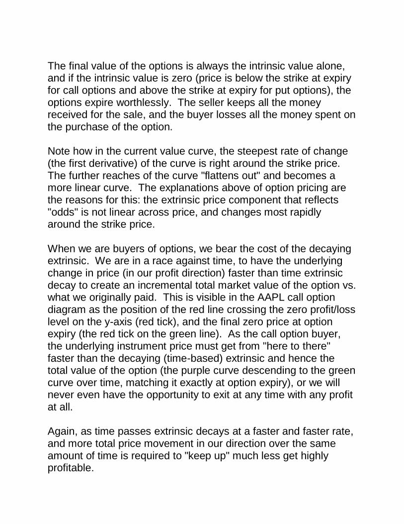
will hold more extrinsic value and hence more potential for profit. By deploying a new spread giving the same odds as the initial spread we can sell enough extrinsic value to be additive to our booked profit plus what we gave up on by exiting early, thus adding to our total profit over the same period (ignoring the commission costs of the option transactions). This takes advantage of early price moves in our favor to "speed up" profit-making overall, instead of always sticking to the pace of the extrinsic value decay. The other advantage of taking partial profits early with an option spread is the elimination of risk. The trade is closed, the profit cash is in our account, and nothing that happens to the price of the underlying matters to us going forward. This is often referred to as "getting off the hot seat". Under what conditions one should exit early is a personal decision, and needs to include your overall expectation for price. Generally, if I am above about 60% of maximum profits, and more than one half of the total time to expiry starting from my purchase date remains, I will often take some or all of my position and "get off the hot seat". Let's now consider a deeper out of the money put spread in AAPL. Here is the profit/loss diagram for ten sold put spreads of AAPL Jan 17'2020, 250/240 (sold 10 250's, bought 10 240's), for a per spread credit of $1.07 (total max profit = $1070 minus commissions). The current price of AAPL is 267.25 (Nov. 30, 2019).

Here we have more skewed odds and win/loss sizes. We have a

73.46% chance of a maximum profit of $1070. We have a

19.24% chance of a loss ranging from -$2755 to -$8930. Thus

our max win to loss ratio is 1070/8930, or 1/8.4.

Note the cross over point price point where the lower of the two

price slice (vertical dashed) lines is placed. This is exactly where

extrinsic value decay shifts from in our favor (growing our profit or

reducing our loss) to against our favor (growing our loss). As

such, it reflects a key level that we might trade against. Should

price reach this level, we stop out at the loss of -$2755. And note

that regardless of how much time remains on the option, it will

always be this loss size.

A critical note: the purple line represents the theoretical value of

the option spread at each price point. In practice, you will find

that you will not be able to close a sold options spread at this

price; you will end up having to pay a bit more, more often than

not. The real world is a bit "worse" than the theory.

The Psychology of Selling Vertical Spreads vs. Direct Purchase

With direct purchase, time becomes immaterial except concerning

our efficiency. It's all about price position now vs. our purchase

price, moment by moment. This creates an "active attitude" for

most traders: we are continually asking ourselves "should I sell

here? here? here?". A common result is of course early selling

that reduces +EV and often significant overtrading.

Compare this to selling spreads. Here, we make money over

time, with a target total. While there are conditions where selling

becomes both "interesting" as in possibly the correct thing to do,

that condition doesn't continually present itself. As a result, we

have a "passive attitude" because that's what assures us our

target profits. Additionally, all our stress about "could I make

more by holding on?" is eliminated! We know exactly the

maximum we can make. And if we are considering exiting early

because we have made 80% of more of our maximum quickly,

doing so is based on either eliminating the position risk and taking

the profit in hand and/or freeing up margin to enter into trades

with even more potential for profit over the same period.

On the loss side, the psychological elements between direct

ownership and sold spreads are very similar. But the benefits to

the trader on the win management side are very significant factors

that make selling spreads appealing and higher +EV for most.

Now we focus on how to identify situations where the actual odds

of price coming into our price zone is much, much lower than the

odds implied by the option pricing. The result is a significant

positive shift in our odds of winning, and hence in our per trade

$EV.

Adding EV Through Market Structure

We'll now shift our focus to the Russell 200 cash index RUT, and

the options available for RUT.

Here's a chart for RUT price action showing what is the most

likely wave count, which is strongly bullish. This count is

supported by a combination of corroborating most likely counts in

other major markets, by historical analogs, and by broad current

economic fundamentals. That said, as explained in detail in

Volume 1, Elliott wave models do not predict a pre-ordained

future. It estimates a non-deterministic, not-pre-ordained future

("anything can happen…and sometimes does"). So we work with

multiple models of potential price action per the Elliott wave rules

and assess which are more and less likely, for reasons of the

structure quality itself, and through additional supportive analysis.

Per the following two charts and the technical and Elliott wave

models presented, we have a very strong expectation of generally

continued rising prices. And should prices not continue to rise,

our next most likely scenario has to be price oscillating in the

upper side of the large price range of the prior 18 months. The

shorter-term momentum is very high; there is significant potential

for continued rapid price movement upward.

Ergo, let's consider the odds of price hitting a lower level at which

we might sell a put spread. Consider the weekly price chart

below, starting with nothing more than the basic MVTrend shown

(the bar coloring: green = strong uptrend, blue = mild uptrend,

purple = neutral trend, orange = mild downtrend, red = strong

downtrend).

There are multiple indicators which in combination give strong

bullish signals for RUT over the near future. First, there is the

break of the price up to and through the descending trend line

over the wide-ranging, highly volatile price swings through most of

2019. Second, there is the price break now (final weekly bar)

above the high of this overall volatile range (in April). Third, the

MVTrend shows a state of strong up (the final bar is green).

MVTI (Morgan Visual Trend Indicator) uses the two quantitative

trend measures of DMI (which includes ADX, DI+, and DI-) and

CCI (commodity channel index) to assess the trend state to one

of five levels as described above. Fourth, the weekly squeeze

indicator (see Vol. 1) has fired by turning off four candles earlier,

with the price rising strongly out of the squeeze. Such squeeze

indicators often indicate 8-9 or more candles of bullish price

action.

One note of mild concern about the price structure is the

approach of price to the 76-78% Fibonacci retrace zone. This

zone is a higher probability area for price to pivot back to down.

Movement up and through this zone would be highly indicative

that price is proceeding upward further, to the 100% retracement

level and potential to the 127% and even the 161%. Additionally,

the price has extended up and through the upper 21-period

volatility channel. Most of the time such excursions are followed

quickly by some kind of reversion back into the channel interior.

Therefore a conservative trade approach would be to wait for

confirmation of further bullish action with a break above these

Fibonacci levels as a trigger to take the position we will soon

describe. Alternatively, waiting for upcoming lows during an

expected immediate small correction is another superior entry

technique.

The next time frame down is the daily chart, and here we include

the wave count.

This wave count positions RUT in the earliest of stages of a minor

3 of an intermediate 3. Price appears to have likely completed a

first low degree i wave up, and is initiating a matching small

degree wave ii. During wave ii a cheaper (higher profit/less risk)

opportunity might arise; the trade example below can probably be

improved upon with more careful stalking of an entry. Do note,

however, that the total extrinsic value received will degrade day

by day, so there is a "rush" to get into a sold premium position.

Note that the most recent correction, modeled as a minor 2 wave

down, bottomed on top of a cluster of Fibonacci retracement

levels that was overall quite shallow, which is also a bullish

indicator.

RUT has some distinct advantages for selling out of the money

vertical spreads. First, because the RUT price is so high, there is

a large amount of "delta" in price between puts of different strikes;

this makes each put spread "efficient" in that we take in more

cash for the commission cost of selling (and later buying back) the

spread.

Secondly, there is a very liquid market for options in RUT quite far

away from the current price level. This gives us added flexibility

for selected exactly how we want to structure our sold spread

without excessive concerns about market liquidity and option

availability at a fair price.

Here's another view of RUT at the daily time frame, focused on

the Fibonacci structure of the swing up. Considering the

Fibonacci structure of RUT's current upswing on the daily chart, it

appears that an option spread at 1505 would give us a stop level

just below the critical 76-78% price retrace level which so often

stops a larger correction. And this level is extremely far away

from where we would think any short term (next 6 weeks)

correction is likely to move to.

The 61.8% shows significant daily candlestick support and

resistance (grey ellipse on the chart). To reach this price level

would require a drop of 6.5% from the recent price high.

We consider a Jan 17, 2020, expiry vertical put spread on RUT,

selling strike 1525 options and buying 1510 options. This

positions our spread just underneath what appears from multiple

perspectives to be both very unlikely to be approached, and

should it be approached, just under strong resistance.

The profit/loss curve diagram for 10 spreads provides $1650 profit

at any expiry price above 1525.

Our stop-loss price level of 1524 (the expiry break-even point) is a

loss of -$4430, giving us a win-loss ratio of 1 to 2.7. Our

theoretical worst-case loss size is $13,350. This is the amount of

margin that will be required through the trade period (about 7

weeks). When we profit, we achieve a $1650/$13350 = 12%

profit on our investment in seven weeks. Should we be able to

operate such a trade successfully with compounding seven times

in a year, we would achieve a total profit of 221%.

However, we won't always win. Using odds based on random

price behavior with volatility as implied by the extrinsic price of the

options, we will achieve full profit 86% of the time (+$1650), we

will achieve a result between full profit and a full stop loss of 1.5%

of the time (-$1306), and a full stop loss 12.5% of the time (-

$4430). Adjusting for a conservative 20% of such stops costing

us a full profit amount (because the price would have recovered to

our profit zone) results in a net per trade average (expected

value) of $677 profit per trade. These figures are before any

adjustment for the incremental edge created by our analysis.

At $677 profit per trade, we have a normalized per trade EV of

$677/$13350 = 5.1%, in seven weeks. If replicated seven times

through the year with compounding, the net EV is 42%. Not bad

for an options trade with "no edge".

Let's now consider the impact of having an edge due to our

analysis. We'll review three possibilities: a small but significant

edge, a moderate edge, and a relatively large edge. For a small

but significant edge, we assume that 15% of all stop out scenarios

are eliminated, and these shift to full profit scenarios. For a

moderate edge, we use 30%. For a relatively large edge, we

assume a 50% reduction in stop-outs.

Here's the EV for each case (and all with the assumption that

20% of stops are at the cost of shifting a full win to a full stop

loss):

- With 15% shift in full stop loss to full win:

$EV = $807

%EV = $807/$13350 = 6.1%

%EV yearly w/compounding (7x): 51%

- With 30% shift in full stop loss to full win:

$EV = $938

%EV = $938/$13350 = 7.1%

%EV year w/compounding (7x): 62%

- With 50% shift in full stop loss to full win:

$EV = $938

%EV = $938/$13350 = 8.3%

%EV year w/compounding (7x): 75%

How much "edge" does our analysis give us? That requires a

vast amount of trading data to estimate empirically; we can only

realistically "guess".

As a more conservative assessment, here's the result assuming

that 30% of stops shift a full win to a full loss and that our analysis

edge shifts 30% of stop out cases under the random volatility

model to full profit; hence, we get exactly what the profit/loss

curve shows us, with every loss at/below the stop point exiting at

our stop loss level of -$4430. In this case, the result is:

- With no net shifting and all full losses at -$4430 (stop level):

$EV = $829

%EV = $938/$13350 = 6.2%

%EV year w/compounding (7x): 52%

Trade Benefits of Selling Out of the Money Premium

Consider the pragmatics of the RUT trade. This trade can be

operated as a "one-shot", meaning, there is zero need to adjust

stops; there is zero need to construct an exit management plan,

including partial incremental exits. Through the adoption of a

simple trade management plan of "close the trade if RUT price

hits stop, else hold to expiry" approach, we eliminate all the risk of

fear and greed-based decision making. If we don't tamper with

it…we cannot "mess it up" by exiting early or exiting late. Simply

put, we know what we get, and we maximize in general by simply

holding to expiry (or exiting instantly at the fixed stop price).

While selling out of the money credit spreads increases odds of

achieving profit, it comes at the cost of a larger loss size, even

under proper stop management. One means of reducing the loss

amount (at the expense of a larger hit to account margin) given

our stop loss practices is to widen the strike spread. The

maximum loss size increases…but this is a don't care for us given

how we will manage the trade. The initial profit/loss curve

flattens, even if it will move down faster and deeper over time.

This can enable a very cheap exit from trades with very large

relative win sizes. This loss reduction increases as we position

our credit spreads at and into the money instead of out of the

money as well.

Spreading Close to the Money

We've focused on selling spreads well away from the current

price (well out of the money). Many setups enable us to be more

aggressive with our spreads. When we have confidence in a

pivot low with nominal structure, lies on top of critical support

levels, and is in the context of higher time frame bullish Elliott

wave structure and up-trending price behavior, we can consider

higher pay off "close spreads" with a more balanced maximum

win to maximum loss size structure.

Here is TSLA at an hourly time frame, as of mid-day 12/7/2020.

Price is clearly in a strong uptrend after breaking out of a very

large 4 wave triangle roughly seven days prior (not shown).

Let's assess selling an "at the money" type spread here with a

short expiration horizon of 12/11 (four days away). The put

spread selected is at 625/565, for a net credit of $1617 for each

sold. Note that the choice of 565 as the strike price for the

purchased put is somewhat arbitrary. Its selection is a means of

selecting the "per spread bet size". If in this situation I wanted to

bet less using a single option spread, I could choose a higher

strike for the purchased put. Hence, there are two ways to "size

bets": widen/reduce the spread amount between the two strikes,

or increase/decrease the number of spreads to be sold.

Here is the profit/loss curve for this trade.

In this case, I would be using a very tight stop around the price

level where the expiry value would be zero, which is about

608.70. The loss size at this price (as of today; it will rise over the

next four days) is about -$732. The max win size is $1617. Note

of course that exit at 608.70 is by no means guaranteed; a market

like TSLA can easily gap open down significantly below this price,

or move very quickly before we can execute and close our

position. When these kinds of "bad situations" occur, there is only

one professional action that can and should be taken: EXIT

IMMEDIATELY. Never "hold and hope" for recovery. Recovery

should be based on future trades, not hoping that this trade, gone

bad, will "get better".

Spreading In the Money

When price action strongly suggests substantial further

movement, it can be highly profitable to go a bit further out in time

and sell spreads that are well "in the money" (at least strike price

of the option being sold is; the option being bought may be at or

out of the money).

Such bets will usually require some price movement in the

direction of the sold option strike to expire with a profit and to

move to or above the sold strike to make a full profit.

There are many analysis tools and setups that give us this

opportunity. For a complete course in this type of analysis, see

my prior book, "Pragmatic Trading: Professional Planning,

Modern Methods".

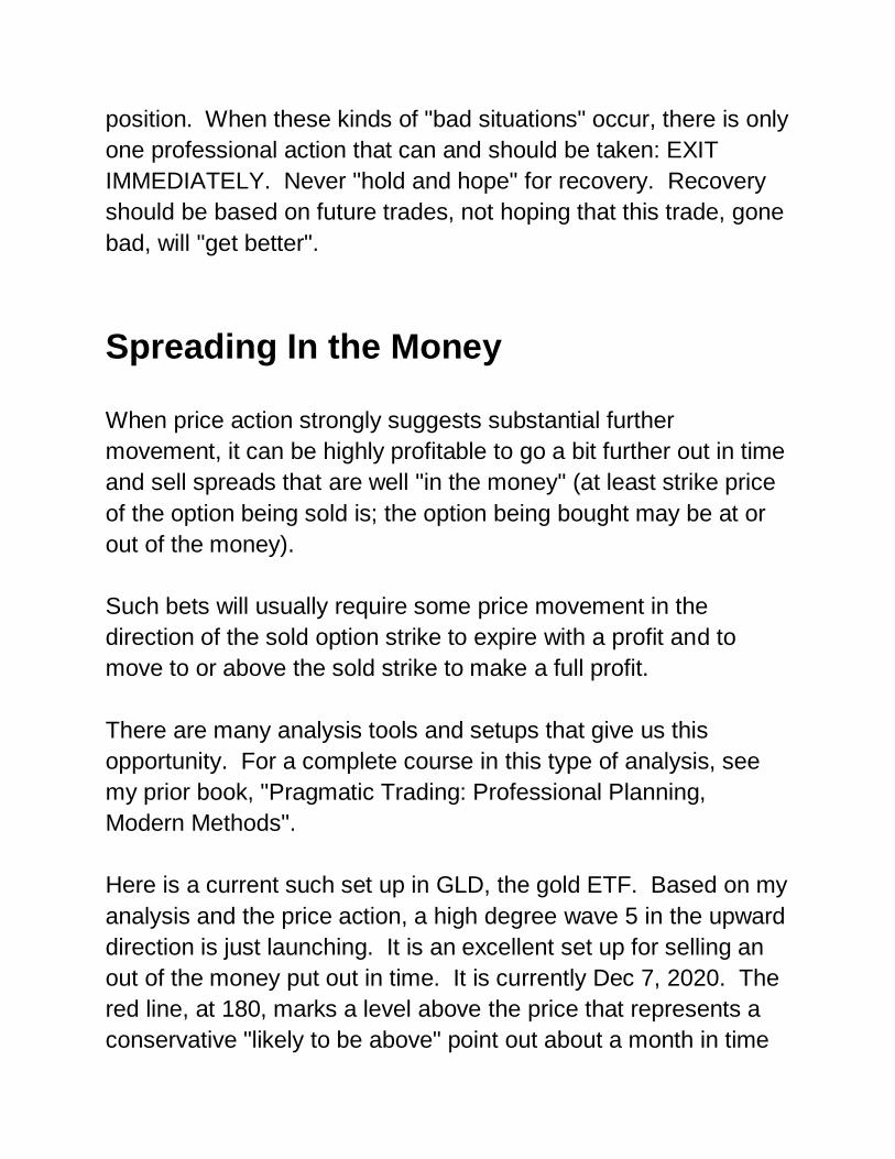
Here is a current such set up in GLD, the gold ETF. Based on my

analysis and the price action, a high degree wave 5 in the upward

direction is just launching. It is an excellent set up for selling an

out of the money put out in time. It is currently Dec 7, 2020. The

red line, at 180, marks a level above the price that represents a

conservative "likely to be above" point out about a month in time

(about 22 more daily candles worth of price action) if this model

continues to play out with [5] wave price movement upward.

To take advantage of this setup, we sell a vertical put spread for

mid-January, with the sold option strike at 180. Here I've selected

a purchased strike of 166, giving a net credit of $619 per sold

spread. This wide delta in strike price significantly lowers the

breakeven point, with the result that the trade opens with price at

a small profit level (but still far from the max profit level which

occurs at GLD at 180). This profit/loss curve is for ten spreads

($6190 total credit).

In this situation, I will be stopping if GLD approaches 170. If on

the other hand, GLD moves upward to 178 or so, I might add

more spreads to the position (which will bring in less credit per

spread, but with greater odds of success).

These kinds of "out of the money" spreads can be used as well in

the longer term. For example, if one believes the equity market

has entered a major new bull phase, selling well out of the money

spreads in market average ETF's like SPY, IWM, DIA, or QQQ for

6-12 months out in time generates tremendous amounts of credit

due to the high extrinsic value of such far dated options.

Bracketing Price with Sold Iron Condors

As should be clear by now, trading by selling option spreads is a

means of trading for profits without requiring any price movement

in a particular direction. The reality of many markets is that most

of the time, price is "going nowhere", just idling in a range. From

an Elliott wave perspective, this is when 2 or 4 waves are

operating. These are consolidation structures.

When a market with a very liquid options market enters a

consolidation phase, one reasonable trade is to sell both an in the

money put spread, and also sell an in the money call spread. The

combination is a "sold" iron condor. The profit/loss curve for such

a condor is shown here for an active trade I have on using this

technique in AMZN. Note that this trade was established about a

week prior, hence, the profit/loss curve in purple is already well

advanced:

Here, on AMZN, I've sold put spreads for Dec 11 at 3075/3050,

and sold call spreads for Dec 11 at 3300/3330. If on Dec 11 at

market close the price of AMZN is between 3075 and 3300, I

profit, and for most of that range, I take "max profit" (I keep all the

money from the sale of both the put and the call spreads).

Here's the current AMZN chart at the hourly time frame that I am

managing this trade to:

The red lines mark the loss levels to both the upside and the

downside. The vertical line is placed at the option expiration point

(end of day trading session on Friday, Dec 7, 2020).

My approach to managing such a trade is the following: first, I

never, ever hold either side until the price reaches one of the red

lines (loss level at expiration for the corresponding spread). If

price approaches either line, I exit that leg of the sold iron condor,

and take the loss "early", with the expectation that I will end up

taking full profit on the other leg. Furthermore, I will often add to

the other leg around the same time (or even earlier, as the price is

heading towards either red line). My worst-case scenario occurs

if the price zooms to one red line, turns, and zooms back to the

other. However, I never set up such a trade for more than two

weeks out to expiration, to minimize that kind of risk.

This kind of trade, when managed well and when put on during

truly "static" market conditions, can be a virtual "no loss" trade, in

that the worst likely scenario is that the loss on one side cancels

out the profit on the other. Managed well, even these scenarios

can generate moderate profits, through the judicious and timely

addition of spreads to the winning side. And in the many cases

where price "stays in the middle" enough to hold both through to

expiration, the payoff is significant.

General Trade Portfolio Considerations

As I have developed my spread selling methods, I have

determined that three critical practices help me achieve consistent

profits. The first is only trading high-quality setups. This entire

subject is covered in rigorous detail in my first book, "Pragmatic

Trading: Professional Planning, Modern Methods". And if there is

one most critical piece of information from that book, it is the

simple adage of "trade with the trend". Trading with the trend

gives you a positive expected value, period. Trying to call tops

and trade short "because the market is extended" or whatever

logic you might come up with is simply trading with a starting

position of negative expectation (average trade return is a loss).

Always trade with the trend. That is course is not enough, but for

the details of how to trade with the trend (it is by no means as

simple as the adage would have you believe), I have to refer you

to my prior text. The proper metaphor for initiating trades is the

hunt: we search for and then stalk our game, and don't fire at our

game (enter our trade) until an exceptional set up develops, and

key price action triggers us to enter our trade. Learn to identify

high-quality setups and triggers that have you trading with trends,

using comprehensive price structure analysis.

The second critical element is to not allow your open spread

positions to get significantly underwater (large open losses). I

often have 10-15 or more open spreads positions. When one

goes "red" in terms of open profit/loss, I watch it very closely and

identify exactly at what underlying price level I will close it for a

small or moderate loss. And I do close it. Without emotion or

concern, "okay, that one is a loser, goodbye". My metaphor for

deploying a large number of sold option spreads is that of a

farmer. I plant a lot of crops by initiating a fair number of sold

spread trades. A few don't immediately grow well, but instead,

wither (go negative in value). I close them and take small losses

before they grow into larger losses due to further falling prices or

due to more time passing. Just as I would pull out the plants from

my farm that grow up weak or diseased: yank 'em out! I let the

healthy ones (sold spreads that move into the profit zone from the

beginning) grow and mature.

The third critical element is to act fast when the overall market

turns against you. If I have ten open spread positions and then

the market moves against me precipitously, I may find my open

profits dropping and dropping. Discretion is the better part of

valor: I unmercifully close my positions, taking what profit I can

salvage, and wait for things to settle out. Allowing winning

positions to all go into losses is not recommended unless the

structure of the sold options allows this because the zero return

price is still yet further away. The cost of closing and then

reselling the option spread later is extremely small, so consider

your nimbleness in the face of adversity to be your real insurance

policy in your trade management.

Earnings Considerations

The impact of approaching earnings is an additional factor that

should be considered when trading with options on single stocks.

That consideration should start with a review of the history of the

change in implied volatility (essentially, change in the intrinsic

component of the price of options) approach and through and just

after earnings announcements. If there is a strong tendency for IV

to rise into earnings, selling extrinsic value through either selling

nake options or selling spreads is contra-indicated. Price may

stay in our full profit zone, but our profit level before expiry may be

well below where it would have been if the IV had stayed stable.

We are in a sense swimming against the tide. Hence, in the

period leading up to an earnings announcement, buying options

spreads can be a more powerful play. And once earnings are

complete, quickly selling option spreads to take advantage of the

high IV and rapid decay is a strategy that adds +EV to our trade.

Conclusions

The benefits of trading options, and particularly of selling option

spreads, has been laid out in detail. For myself, selling option

spreads is my bread and butter trade. I strongly prefer not having

to sweat the question of "when do I sell?" all the time. I like to

maintain multiple open positions, and I like a "board" that shows

open profit levels on all of them, or only small/moderate and

reasonable at this point losses (usually meaning if price stays

where it is, at expiry the position will be profitable). For myself,

it's a much more sane, and overall profitable means of trading. I

know what I'm targeting for "income", and I'm not dependent on

price movement per se to achieve it. I find this method to be a

vastly superior means of extracting consistent profits from the

equity markets.

May the trading Gods smile upon you! Best of success in your

options trading journey.

If you found value in this text and would like to learn the details of

price structure analysis and trade setups and management,

please consider the purchase of Volume 1 of this series:

Pragmatic Trading: Professional Planning, Modern Methods. You

can find it on Amazon and at http://www.specktrading.com/.