pragmatic method based on intelligent big data analytics
TRANSCRIPT

Pragmatic Method Based on Intelligent BigData Analytics to Prediction Air Pollution
Samaher Al_Janabi(&) , Ali Yaqoob, and Mustafa Mohammad
Department of Computer Science, Faculty of Science for Women (SCIW),University of Babylon, Babylon, Iraq
Abstract. Deep learning, as one of the most popular techniques, is able toefficiently train a model on big data by using large-scale optimization algo-rithms. Although there exist some works applying machine learning to airquality prediction, most of the prior studies are restricted to several-year dataand simply train standard regression models (linear or nonlinear) to predict thehourly air pollution concentration. The main purpose of this proposal is designpredictor to accurately forecast air quality indices (AQIs) of the future 48 h.Accurate predictions of AQIs can bring enormous value to governments,enterprises, and the general public -and help them make informed decisions. WeWill Build Model Consist of four Steps: (A) Determine the Main Rules (con-tractions) of avoiding emission (B) Obtaining and pre-processing reliabledatabase from (KDD CUP 2018) (C) Building Predator have multi-level basedon Long Short-term Memory network corporative with one of optimizationalgorithm called (Partial Swarm) to predict the PM2.5, PM10, and O3 con-centration levels over the coming 48 h for every measurement station. (D) Toevaluate the predictions, on each day, SMAPE scores will be calculated for eachstation, each hour of the day (48 h overall), and each pollutant (PM2.5, PM10,SOx, CO, O3 and NOx). The daily SMAPE score will then be the average of allthe individual SMAPE scores.
Keywords: Air pollutant prediction � Big data � Prediction � LSTM � PSO
1 Introduction
The proposed title deals with the study of gases that cause air pollution. The proposedtitle deals with the study of gases that cause air pollution. Air pollution has become aserious threat to large parts of the Earth’s population [1]. Air pollution control hasattracted the attention of governments, industrial companies and scientific communi-ties. There are two sources of air pollution: the first source is natural sources such asvolcanoes, forest fires, radioactive materials, etc. The second source is industrialsources produced by human activities such as factories, vehicles, remnants of war andothers. These pollutants produce different types of gases, including sulfur oxides (SOx),carbon monoxide (CO), nitrogen oxides (NOx) and ozone (O3). Another type ofcontaminant is PM2.5 (particulate matter), a mixture of compounds (solids and liquiddroplets), the most dangerous types of contaminants cause cardiovascular disease plus
© Springer Nature Switzerland AG 2020Y. Farhaoui (Ed.): BDNT 2019, LNNS 81, pp. 84–109, 2020.https://doi.org/10.1007/978-3-030-23672-4_8

pollutant PM10. This work calculates concentrations of air pollutants (6 types of airpollution above) using a predictive model capable of handling large data efficiently andproducing very accurate results. Therefore, a long short-term memory model using theswarm algorithm was used and developed. So that the network is trained to concentratethis polluted air on a number of stations and every hour and the results are evaluatedusing Root Mean error the scale of assessment so that this model can predict within thenext 48 h. These data are analyses, conversion, testing, modelling, accurate informationmining, restructuring and storage. This information helps us make decisions aboutthese data and takes them across several stages before they are entered into the net-work. It is the data collection phase of the different version. This is the data problem tobe expected. Are the determinants and stage of understanding the nature of these data inthemselves? This data is a very important stage where the data we deal with containsmissing data processed by each column and then these data are entered after analysis ina model developed and evaluated by SMAPE.
The remind of this paper organization as follow. Section 2 show the related work.Section 3 explain the main concept used to handle this problem. Section 4 show theprototype of pragmatic system while Sect. 5 show the results. Finally, Sect. 6description the discussion and conclusion of the problem statement.
2 Related Works
The issue of air quality prediction is one of the vital topics that are directly related tothe lives of people and the continuation of a healthy life in general. Since the subject ofthis thesis is to find a modern predictive way to deal with this type of data that is hugeand operates within the field of data series. Therefore, in this part of the thesis, we willtry to review the works of the former researchers in the same area of our problem andcompare these works in terms of five basic points, namely the database used. Themethods to assess the results, the advantages of the method, and their limitations.
Bun et al. [1] used “deep recurrent neural network (DRNN)” that is reinforced withthe novel pre-training system using auto-encoder principally design for time seriesprediction. Moreover, sensors chosen is performed within DRNN without harming theaccuracy of the predictions by taking of the sparsity found in the system. The methodused to solve particulate matter (PM2:5) that is one of the air populations. this methodreveals results in more accuracy than the poor performance of the “Noise reduction(AE)”. Evaluation the results based on four measures: “Root mean square error(RMSE), precision (P), Recall (R) and F-measure (F)”. Our work is similar that workby using the same technique RNN while we predicate based on “long short-termmemory”.
Samaher et al. [2] the researcher found in this work the hybrid system uses “geneticneural computing (GNC)” to analyze and understand the resulting data from theconcentration of dissolved gases. Where it is used in four subgroups for the purpose ofanalysis and assembly based on the C57.104 Specified by “IEEE” using “GA”. Isinserted the clustering data into the neural network for the purpose of predictingdifferent types of errors. This hybrid system generates decision rules which identify theerror accurately. There are two measures used in this work are: “The Davies–Bouldin
Pragmatic Method Based on Intelligent Big Data Analytics 85
(DB) index and MSE”. This work has proven to provide less cost to solve the problem.And through this method facilitates the process of prediction and identify moreaccurate ideas through the analysis of errors and ways to address them. This work issimilar to our work in terms of using neural networks but the difference is using a”Swarm” algorithm with “LSTM”.
Xiang et al. [3] used model “spatiotemporal deep learning (STDL)”-based on airquality prediction method. It used a “stacked autoencoder (SAE)” method to extractinherent air quality characteristics, in addition, it is trained in a greedy layer-wisemethod. it compared your’ model with traditional time series prediction models, themodel can predict the air quality of all stations at the same time and shows the temporalstability in all seasons. In addition, a comparison with the “spatiotemporal artificialneural network (STANN)”, “autoregression moving average (ARMA)”, and “supportvector regression (SVR)” models demonstrates. The results of that model evaluation bythree measures are “RMSE”, “MAE” “MAPE”. Our work is similar that work by usingthe same technique RNN to prediction the air quality index but we deal with huge data,“long-short-term memory” (“LSTM”) to enhance network work.
Xiang et al. [4] used “long short-term memory neural network” extended(“LSTME”) model which is the association of spatial-temporal links to predict theconcentration of air pollutants. Long-term memory layers (LSTM) have been used toautomatically extract potential intrinsic properties from historical air pollutants data,and assistive data, Contains meteorological data and timestamp data, has been incor-porated into the proposed model to improve performance. This technique evaluation bythree measures “RMSE”, “MAE” and “MAPE”. A comparison with the “spatiotem-poral artificial neural network (STANN)”, “autoregression moving average (ARMA)”,and “support vector regression (SVR)” models demonstrates. Our work is similar thatwork by using long-short-term memory (“LSTM”) as part of the repeated neural net-work structure. While differ by using another evaluation measure.
Osama et al. [5] “shown a new deep learning-based ozone level prediction model,which considers the pollution and weather correlations integrally. This deep learningmodel is used to learn ozone level features, and it is trained using a grid searchtechnique. A deep architecture model is utilized to represent ozone level features forprediction. Moreover, experiments demonstrate that the proposed method for ozonelevel prediction has superior performance. The outcome of this study can be helpful inpredicting the ozone level pollution in Aarhus city as a model of smart cities forimproving the accuracy of ozone forecasting tools”. Results of that model evaluationbased on “RMSE”, “MAE”, “MAPE”, squared “R2” and correlation coefficient. Ourwork will also use memory in (“LSTM”) for the processing large data, but differ byfinding the optimal structure of that neural network by partial swarm algorithm.
Lifeng et al. [6] the author found that obtaining the best air quality prediction usesthe GM model (1.1) the fractional order accumulation (FGM (1.1)) to find the Expectedthe average annual concentrations of “PM2.5, PM10, SO2, NO2, and 8-h O3 And O-24 h”. The measure used in this search is “MAPE”. Using the method of “FGM (1.1)”obtained much higher than the traditional GM model (1.1), the average annual con-centrations of “PM2.5, PM10, SO2, NO2, O8-O3, and O3 24-h” will decrease from2017 to 2020. This work is similar to our work in terms of predicting the concentration
86 S. Al_Janabi et al.

of air pollutants and finding ways to address them, but the difference in terms of themethod of prediction using “LSTM”.
Olalekan et al. [7] in this work the method was used Sensor measurement: SNAQboxes and network deployment, Sensor measurement validation, Source apportionmentto create a predictive model for modeling (ADMS-Airport), the concentration of pol-lutants to determine the air quality model. The results showed in this study can beapplied in many environments that suffer from air pollution. Which will reduce thepotential health effects of air quality and the lowest cost, as well as monitor greenhousegas emissions? This work is similar to our work to determine the concentration of airpollutants but the method used for our work is “LSTM –RNN”.
Congcong et al. [8] in order to extract high temporal-spatial features have been usedby the Merge of the “convolutional neural network (CNN)” and “long short-termmemory neural network (LSTM-NN), and meteorological data and aerosol data werealso Merge, in order to refinement model prediction performance. The data collectedfrom 1233 air quality monitoring stations in Beijing and the whole of China were usedto verify the effectiveness of the proposed C-LSTME model. The results show that thepresent model has achieved better performance than current state-of-the-art Tech-nologies for different time predictions at various regional and environmental scales.This technique evaluation by three measures “RMSE”, “MAE” and “MAPE”. Ourwork used “LSTM” through RNN but after fined the best structure of that network. Itdiffers by using another evaluation measures.
Zhigen et al. [9] the prediction method was based on “classification and regressiontree (“CART”)” and was combined with the “ensemble extreme learning machine(EELM)” method. Subgroups were created by dividing datasets by creating a shallowhierarchy tree by dividing the data set through “CART”. Where at each node of the tree“EEL Models” are done using the training samples of the node, to minimize theverification errors sequentially to all the tree sub-trees by identifying the numbers ofhidden intestines where each node is considered as root. Finally, EEL models for eachpath of the leaf is compared to the root on each leaf and only one path is selected withthe smallest error checking the leaf. The measures that used are RMSE and MAPE.This method proved that the experimental results of the measurements used: canaddress the global-local duplication of the method of prediction in each leaf, “CART-EELM” work better than the models “RF, v-SVR, and EELM”, “CART-EELM” alsoshows superior performance compared “EELM and K-means-EELM seasonal”. Ourwork is similar to this work using the same set of six data for air pollution “(PM2.5,O3, PM10, SO2, NO2, CO)”, but we differ in terms of the mechanism of reducing airpollutants where we use the RNN method.
Hongmin et al. [10] using a new air quality forecasting method, and proposing anew positive analysis mechanism that includes complex analysis, improved predictionunits, pre-treatment data, and air quality control problems. This system analyzes theoriginal series using the entropy model and data processing process. The “MOMVO”algorithm was used to achieve the required standards and “LSSVM” to achieve the bestaccuracy in addition to stable prediction. There are three ratings used in this work are:“RMSE”, “MAE” and “MAPE”. The result of the application of the proposed methodon the data set showed a good performance in the analysis and control of air quality, inaddition to the approximation of values with high precision. Our work used the same
Pragmatic Method Based on Intelligent Big Data Analytics 87

Tab
le1.
Com
pare
amon
gtheprevious
works
Nam
eDataset/database
Method
Evaluation
Advantage
Bun
etal.
[1]
Airqu
ality
index
“(AQI)”
http://uk-air.defra.
gov.uk
“(DRNN)”
that
isenhanced
with
anovelpre-training
methodusingauto-encoder
•“(RMSE
)”•“(P)”
•“(R)”
•“(F)”
1-The
numericalexperimentsshow
thatDRNNwith
ourp
roposed
pre-training
methodissuperior
towhenusingacanonicalanda
state-of-the-artauto-encoder
training
methodwhenappliedto
time
series
predictio
n.The
experimentsconfi
rmthat
whencompared
againstthePM
2:5predictio
nsystem
VENUS
2-NNwas
know
nas
“(RNN)”,incontrastwith
“(FN
N)”,h
asbeen
show
nto
exhibitvery
good
performance
inmodelingtemporal
structures
andhasbeen
successfully
appliedto
manyreal-w
orld
prob
lems
Samaher
etal.[2]
•“(GNC)”
•“B
PNN”
•“M
SE”
•“(DB)”
Thisworkhasprov
ento
prov
ideless
costto
solvetheproblem.
And
throughthismethodfacilitates
theprocessof
predictio
nand
identifymoreaccurate
ideasthroug
htheanalysisof
errors
and
waysto
addressthem
Xiang
etal.[3]
Airqu
ality
using
PM2.5
(http
://datacenter.
mep.gov.cn/).
1-“(ST
DL)”
basedairqu
ality
predictio
nmethod
2-“(SA
E)”
•“(RMSE
)”•“(MAE)”
•“(MAPE
)”
3-Com
paredwith
traditional
timeseries
airquality
predictio
nmodels,ourmodel
was
able
topredicttheairquality
ofall
monito
ring
stations
simultaneously,
anditshow
edsatisfactory
season
alstability.Weevaluatedtheperformance
oftheproposed
methodandcompareditwith
theperformance
ofthe“STANN”,
“ARMA”,
and“SVR”mod
elsandtheresults
show
edthat
the
prop
osed
methodwas
effectiveandou
tperform
edthecompetitors
Xiang
etal.[4]
Airqu
ality
using
PM2.5
(http
://datacenter.
mep.gov.cn/)
•“(LST
M)”
•“(RMSE
)”•“(MAE)”
•“(MAPE
)”
The
“LST
ME”mod
eliscapableof
mod
elingtim
eseries
with
longtim
edependencies
andcanautomatically
determ
inethe
optim
umtim
elags.Toevaluate
theperformance
ofourproposed
model,Com
paredwith
Sixdifferentmodels,includingour
“LST
ME”,
thetradition
al“L
STM”“N
N”,
the“STDL”,
the
“TDNN”,
the“A
RMA”andthe“SVR”mod
els
Osama
etal.[5]
City
pulsedataset.
(ftp://http://iot.
ee.surrey.ac.uk:)
1-Deeplearning
approach
2-In-M
emorycomputin
g•“(RMSE
)”•“(MAE)”
•“(MAPE
)”•“(R2 )”
•“(r)”
The
proposed
methodisevaluatedon
cityplusedatasetand
comparedwith
SVM,NN,andGLM
mod
els.thecomparison
results
show
that
theprop
osed
mod
elisefficientandsuperior
ascomparedto
alreadyexistin
gmod
els
(con
tinued)
88 S. Al_Janabi et al.

Tab
le1.
(con
tinued)
Nam
eDataset/database
Method
Evaluation
Advantage
Lifeng
etal.[6]
BBC,20
13.Beijin
gSm
og:w
henGrowth
Trumps
Lifein
China.
www.bbc.com
/new
s/magazine-21
1982
65
“FGM(1,1)”
•“R
MSE
”•“M
APE
”Using
themetho
dof
“FGM
(1.1)”
obtained
muchhigher
than
the
traditional
GM
model
(1.1),theaverageannual
concentrations
of“PM2.5,
PM10
,SO
2,NO2,
O8-O3,
andO324
-h”will
decrease
Olalekan
etal.[7]
•“SNAQ
boxesandnetwork
deploy
ment”
•Sensor
measurement
valid
ation.
Source
apportionm
ent
The
results
show
edin
thisstud
ycanbe
appliedin
many
environm
entsthat
suffer
from
airpo
llutio
n
Congcon
get
al.[8]
Hou
rlyPM
2.5
concentrationdata
from
1233
air
quality
mon
itoring
stations
inChina
collected
from
Janu
ary1,
2016
,to
Decem
ber31
,20
17,
wereacquired
from
theMinistryof
Env
iron
mental
Protectio
nof
China
(http
://datacenter.
mep.gov.cn/).
combinatio
nof
the“(CNN)”
and“(LST
M-N
N)”
•“(RMSE
)”•“(MAE)”
•“(MAPE
)”
(1)The
additio
nof
PM2.5inform
ationfrom
neighb
oringstations,
which
contributesto
thespatialityof
thedata,canconsiderably
improvethepredictio
naccuracy
ofthemodel
(2)The
supplementof
auxiliary
data
canhelp
predictsudden
changesin
airquality
,therebyim
provingthepredictio
nperformance
ofthemodel.Moreover,comparedto
meteorological
data,the
“AOD”datacontributesmoreto
theaccuracy
ofthemod
el(3)The
presentmod
elcanefficiently
extractmoreessential
spatiotemporalcorrelationfeatures
throughthecombinatio
nof
“3D-CNN”andstateful
“LST
M”,therebyyielding
higher
accuracy
andstability
forairquality
predictio
nof
differentspatiotemporal
scales
(contin
ued)
Pragmatic Method Based on Intelligent Big Data Analytics 89

Tab
le1.
(con
tinued)
Nam
eDataset/database
Method
Evaluation
Advantage
Zhigen
etal.[9]
Yanchengcity,
which
ison
eof
the
13citiesun
derthe
direct
administration
ofJiangsuProv
ince,
China.Y
anchengcity
spansbetween
northern
latitude
32°34′–34
°28′,
easternlong
itude
119°27
′–12
0°54′
“CART”and“E
ELM”
•“(RMSE
)”•“(MAPE
”)The
experimentalresults
ofthemeasurementsused:canaddress
theglobal-local
duplicationof
themethodof
predictio
nin
each
leaf,“C
ART-EELM”workbetterthan
themod
els“R
F,v-SV
R,
andEELM”,
“CART-EELM”also
show
ssuperior
performance
compared“E
ELM
andK-m
eans-EELM
season
al
Hon
gmin
etal.[10]
The
datasetsfrom
eightsitesin
China.
(http
s://d
ata.epmap.
org)
•“L
SSVM”
•“M
OMVO”
•“(RMSE
)”•“(MAE)”
•“(MAPE
)”
The
applicationof
theproposed
methodon
thedata
setshow
eda
good
performance
intheanalysisandcontrolof
airqu
ality
,in
additio
nto
theapproxim
ationof
values
with
high
precision
90 S. Al_Janabi et al.

evaluation measures but it differs by using “LSTM” through RNN but after fined thebest structure of that network.
Table 1 Shown the compare among the previous works based on five points aretypes of dataset, methodology used, evaluation measures, and advantages.
3 Main Concept
3.1 Big Data
There are three types of data. The first type is small data: these data are not subject tonormal distribution and therefore cannot be determined and difficult to predict due totheir small size and less than 30 samples, the second type is the normal data is the mostcommon data that is organized in the table consists of columns and rows, For large datathat we will deal with in our work. These big data cannot be handled in the traditionalway due to their large size. From TB to ZB, these big data are either structural, semi-structured or unorganized. In large data, there are three conditions that must be met:First, the existence of available data called the data domain has three characteristics ofvolume, Velocity and Variety. The second condition: There is a statistic for this datacalled (statistical domain), which has three characteristics are Veracity, Variability andValidity. The third condition is the existence of the beneficiary of this data called(intelligence analysis domain) which has three characteristics of Visibility, value andVerdict [11].
3.2 Big Data Analysis Stages
The attention to large data has become of great importance to many organizations andcompanies over the last few years so many technologies have been developed to meetthe challenges of dealing with huge data The process of analysis of the statementthrough several stages: the data deployment stage is the stage of data collection fromdifferent sources, the stage of understanding the problem: the phase of understandingthe problem of data and the problem of this proposal are the gases and vehicles thatresult from air pollution, data exploration stage: After understanding the data problem,Itself. Does this data contain missing data? Is this data of an integer type, type ofcharacters, or mixture between them?, data pre-processing stage This is a veryimportant stage because the data we deal with contains missing data to be processed byeach column in addition to the filtering of data. After processing the data, we need tobuild a predictive model for this data, that called the data modelling stage and thenevaluate the data using one of the different measurements called the data assessmentstage [12].
3.3 Deep Learning
It is a new research field that examines the creation of theories and algorithms thatallow the machine to learn by itself by simulating neurons in the human body. And oneof the branches of science that deals with artificial intelligence science. From an
Pragmatic Method Based on Intelligent Big Data Analytics 91

Automated Learning Science branch, most in-depth learning research focuses onfinding methods to derive a high degree of strippers by analyzing a large data set usinglinear and nonlinear mutants. “Discoveries in this area have proven significant, rapidand effective progress in many areas, including face recognition, speech recognition,computer vision, and natural language processing.” Deep learning is a branch oflearning, which is a branch of artificial intelligence. Where deep learning is divided intothree basic categories: Deep networks under supervision or deep discriminationModels, deep unsupervised networks or giant models, deep hybrid networks” [13].
3.4 Prediction
Prediction is the process of studying and making guesses about future time events usingspecific mechanisms across time periods and different spatial intervals. It is a way forpolicymakers to develop plans to address future risks. The process of prediction goesthrough several stages, the most important of which are: determining the purpose offorecasting, gathering the data needed for a predictable phenomenon, analyzing andextracting data, and selecting the appropriate model or mechanism to predict thephenomenon under consideration and to take the appropriate decision. The forecastingprocess is capable of predicting the state of data based on advance data, a necessarystep to give very low error rates [14] (Fig. 1).
3.5 Air Pollution
Pollution is a serious concern that has attracted the attention of industrial companies,the international community and scientific and health communities because it containssubstances harmful to the lives of humans and other living organisms. These pollutantsproduce different types of concentrations that cause air pollution, including sulfurdioxide SO2, Nitrogen Dioxide gas NO2, Carbon monoxide gas CO, Ozone gas O3,Vehicles with mixed composition PM2.5 and PM10. Predicting concentrations thatcause air pollution is very important for health community organizations and to launchan early warning and decide on these concentrations [15].
Fig. 1. Main Types of Machine Learning Techniques [19]
92 S. Al_Janabi et al.
4 A Prototype of Smart Air Quality Prediction Model(SAQPM)
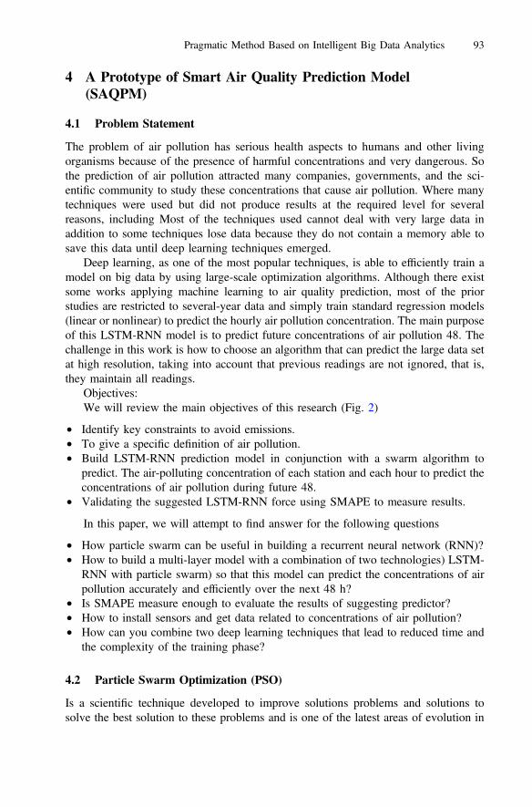
4.1 Problem Statement
The problem of air pollution has serious health aspects to humans and other livingorganisms because of the presence of harmful concentrations and very dangerous. Sothe prediction of air pollution attracted many companies, governments, and the sci-entific community to study these concentrations that cause air pollution. Where manytechniques were used but did not produce results at the required level for severalreasons, including Most of the techniques used cannot deal with very large data inaddition to some techniques lose data because they do not contain a memory able tosave this data until deep learning techniques emerged.
Deep learning, as one of the most popular techniques, is able to efficiently train amodel on big data by using large-scale optimization algorithms. Although there existsome works applying machine learning to air quality prediction, most of the priorstudies are restricted to several-year data and simply train standard regression models(linear or nonlinear) to predict the hourly air pollution concentration. The main purposeof this LSTM-RNN model is to predict future concentrations of air pollution 48. Thechallenge in this work is how to choose an algorithm that can predict the large data setat high resolution, taking into account that previous readings are not ignored, that is,they maintain all readings.
Objectives:We will review the main objectives of this research (Fig. 2)
• Identify key constraints to avoid emissions.• To give a specific definition of air pollution.• Build LSTM-RNN prediction model in conjunction with a swarm algorithm to
predict. The air-polluting concentration of each station and each hour to predict theconcentrations of air pollution during future 48.
• Validating the suggested LSTM-RNN force using SMAPE to measure results.
In this paper, we will attempt to find answer for the following questions
• How particle swarm can be useful in building a recurrent neural network (RNN)?• How to build a multi-layer model with a combination of two technologies) LSTM-
RNN with particle swarm) so that this model can predict the concentrations of airpollution accurately and efficiently over the next 48 h?
• Is SMAPE measure enough to evaluate the results of suggesting predictor?• How to install sensors and get data related to concentrations of air pollution?• How can you combine two deep learning techniques that lead to reduced time and
the complexity of the training phase?
4.2 Particle Swarm Optimization (PSO)
Is a scientific technique developed to improve solutions problems and solutions tosolve the best solution to these problems and is one of the latest areas of evolution in
Pragmatic Method Based on Intelligent Big Data Analytics 93

the field of artificial intelligence, developed by the world (Kennedy and Eberhart) in1990, and the idea of PSO of the behavioral and social behavior of bird droppingsthrough the idea of research About the food, where the bird squadron are looking forfood from one place to another and that some birds in the squadron have the ability todistinguish the smell of food in a strong and effective with information for these birdsabout the best place to eat because some birds send information among themselvesduring the search process and Inspection of the best place for food, when the bird flockis explored for a good place for food quality, these birds use this place to get betterfood. Thus, the work of the swarm algorithm is the search process and replicationprocess of the best solutions within the specific research area. The PSO algorithm canbe used to solve optimization problems and problems that change by the time [16, 17].
4.2.1 Basic Components of the Bird Swarm Algorithm (PSO)The swarm algorithm consists of the numbers of the population of the swarm calledparticles. Symbolizes them (n) which consists of n = (n1, n2, …, ni) which moveswithin the swarm of the search space determined by the type of problem which is multi-dimensional and the search for good initial solutions. Particles depend on their ownexpert and also rely on the experts and experiences of neighboring particles within theswarm, The PSO algorithm is randomly assigned to the number of particles of thesquadron in the search area. The use of the squadron particles when creating the PSOalgorithm depends on the velocity of the particles that comprise Vt
i ¼ ðVt1;V
t2; . . .;V
ti Þ
the location of the particles that are composed of Xti ¼ Xt
1;Xt2; . . .;X
ti
� �; where it is
determined based on the previous cases of the best location of the particle itself andsymbolizes it Pt
best;i, The best location of the particles in the entire swarm symbolizes it
Fig. 2. Block Diagram of Proposed DLSTM-RNN
94 S. Al_Janabi et al.

Gtbest;i, Depending on the dimensions of problem d, consisting of (d1, d2,…dj), The
speed and location of each particle are adjusted according to the following equations:
Vtþ 1i ¼ ðVt
1 þ c1rt1 Pt
best;i � Xti
� �þ c2r
t2 Gt
best;i � Xti
� �ð1Þ
Xtþ 1i ¼ Xt
i þVti ð2Þ
Where:
Vti : Particle velocity i in swarm in dimension j and frequency t.
Xti : The location of the particle i in a swarm in dimension j and frequency t.
c1: acceleration factor related to Pbest.c2: Acceleration factor related to gbest.rt1, r
t2: random number between 0 and 1.
t: Number of occurrences specified by type of problem.Gt
best;i: gbest position of swarmPtbest;i: pbest position of particle.
Activation function
# hidden layer[ 2 -10 ]
# nodeOf hidden layer
[ 1 – 5 ]
Weight Of W Weight of U
Find Optimal Structure of LSTM-RNN By Particle Swarm Optimization
HyperbolicFunction
PolynomialFunction
Weight of input activation (Wa)
Weight of inputgate (Wi)
Weight of Forget gate
Weight of Out-put gate (Wo)
Weight of input activation Ua
Weight of inputgate Ui
Weight of Forget gate Uf
Weight of Output gate Uo
f) (W
Fig. 3. PSO algorithm is to optimize the LSTM-RNN
Pragmatic Method Based on Intelligent Big Data Analytics 95

The aim of the PSO algorithm is to optimize the structure of LSTM-RNN fromdetermined the best activation function for each layer, determined number of hiddenlayers in network, number of neurons in each hidden layer, and the optimal weightsbetween each layer and the layer next it as described in the diagram (Fig. 3 andTables 2 and 3):
Table 2. Hyperbolic Functions with discretion [20]
Hyperbolic functionName of hyperbolic function #variable Function
Sinh One F(x) = ex�e�x
2
Cosh One F(x) = ex þ e�x
2
Tanh One F(x) = ex�e�x
ex þ e�x
Sinh−1 One F(x) = 2ex�e�x
Cosh−1 One F(x) = 2ex þ e�x
Tanh−1 One F(x) = ex þ e�x
ex�e�x
Where: x is input and F(x) is output.
Table 3. Polynomial Functions with discretion [20]
Polynomial functionsName of polynomial function #variable Function
Linear One F(x) = p1+p2*x1Linear Tow F(x) = p1+p2*x1+p3*x2Linear Three F(x) = p1+p2*x1+p3*x2+p4*x3Quadratic One F(x) = p1+p2*x1+p3*x1^2Quadratic Tow F(x) = 1+p2*x1+p3*x1^2+p4*x2
+p5*x2^2+p6*x1*x2Cubic One F(x) = p1+p2*x1+p3*x1^2 +p4*x1^3Product Tow F(x) = p1+p2*x1*x2Ratio Tow F(x) = p1+p2*(x1/x2)Logistic One F(x) = p1+p2/(1+ exp(p3*(x1-p4)))Log One F(x) = p1+p2*Log(x1+p3)Exponential One F(x) = p1+p2*exp((p3*(x1+p4))Asymptotic One F(x) = p1+p2/(x1+p3)
Where:x is inputf(x) is outputp1, p2, p3, p4: is constants
96 S. Al_Janabi et al.

Algorithm #1: PSO [21]
1. Set of parameters2. A: Population of agents, pi: Position of agent ai in the solution space, f : Objec-
tive function 3. vi : Velocity of agent’s ai , V(ai): Neighborhood of agent ai (fixed)4. [x*] = PSO()5. P = Particle_Initialization()6. For i=1 to it_max7. For each particle p in P do8. fp = f(p)9. If fp is better than f(pBest)10. pBest = p11. End12. End13. gBest = best p in P14. For each particle p in P do15. # v = v + c1*rand*(pBest – p) + c2*rand*(gBest – p)16. # p = p + v17. End18. End
4.3 Long Short-Term Memory (LSTM)
LSTM was proposed in 1997 by Sepp Hochreiter and Jürgen Schmidhuber. Byintroducing Crossover Fixed Error (CEC) modules, LSTM deals with gradient andburst problems. The initial version of the block included LSTM cells, input and outputgateways. LSTM achieved record results in natural language text compression, unau-thorized handwriting recognition and won the Handwriting Competition (2009). LSTMnetworks were a key component of the network, which achieved a standard audio errorrate of 17.7% over the traditional natural speech data set (2013). (LSTM) are units ofthe Recurrent Neural Network (RNN). The RNN is often called LSTM (or LSTMonly). The common LSTM module consists of a cell, an input port, an output port, anda forgotten gateway. The cell remembers values at random intervals and the three gatesregulate the flow of information inside and outside the cell. LSTM networks are wellsuited for classifying, processing and predicting predictions based on time series data,where there may be an unknown delay for important events in a time series. LSTMshave been developed to deal with fading and fading problems that can be encounteredwhen training traditional RNNs. The relative lack of sense of gap length is the LSTMfeature on RNNs, Hidden Markov models and other sequential learning methods inmany applications [18].
Pragmatic Method Based on Intelligent Big Data Analytics 97

4.3.1 LSTM Architecture and AlgorithmThere are many structures for LSTM modules. The common structure of a cell (thememory part of the LSTM module) and three “organizations”, usually called portals,consist of the flow of information within the LSTM module: an input gateway, anoutput gateway, and a forgotten gateway. Some differences in the LSTM module do notcontain one or more of these portals or may have other portals. For example, duplicateunits do not contain portals (GRUs) on the output portal.
Intuitively, the cell is responsible for tracking dependencies between elements inthe input sequence. The input gateway controls the extent to which a new value isflowing into the cell. The ny gate controls how long a value in the cell and the outputgateway controls how much the value in the cell is used to calculate the output activatethe LSTM module. LSTM port activation function is often the logistics function.
There are connections to and from LSTM portals, a few of which are frequent. Theweights of these links, which must be learned during training, determine how the gateswork.
4.3.2 The Variables in LSTM – RNNThis algorithm required setup multi variables at the beginning then through it work willupdate these variables by apply computation operations. as shown below (Fig. 4):
Fig. 4. LSTM cell
98 S. Al_Janabi et al.

Step 1: The forward componentsStep 1.1: Compute the gates:Input activation:
at ¼ tanh Wa: Xt þ Ua: outt�1 þ bað Þ ð3Þ
Input gate:
it ¼ r WI: Xt þ Ui: outt�1 þ bið Þ ð4Þ
Forget gate:
ftr Wf :Xt þ Uf : outt�1 þ bfð Þ ð5Þ
Output gate:
otr Wo: Xt þ Uo: outt�1 þ boð Þ ð6Þ
Then fined:Internal state:
State = at � it þ ft � statet�1 ð7Þ
Output:
outt ¼ tanh stateð Þ � ot ð8Þ
Where
Gate St =
atitftot
264
375, W =
Wa
WiWf
Wo
264
375, U =
Ua
UiUf
Uo
264
375, b =
babibfbo
264
375
Step. 2: The backward components:Step 2.1. FindDt the output difference as computed by any subsequent.DOUT the output difference as computed by the next time-step
doutt ¼ Dt þDoutt ð9Þ
dstatet ¼ doutt � ot � 1� tanh2 statetð Þ� �þ dstatetþ 1 � ftþ 1 ð10Þ
Pragmatic Method Based on Intelligent Big Data Analytics 99

Step 2.2: Gives:
dat ¼ dstatet � it � ð1� a2t Þ ð11Þdit ¼ dstatet � at � it � ð1� itÞ ð12Þ
dft ¼ dstatet � statet�1 � ft � ð1� ftÞ ð13Þ
dot ¼ doutt � tanhðstatetÞ � ot � ð1� otÞ ð14Þ
dxt ¼ Wt:dstatet ð15Þ
doutt�1 ¼ Ut:dstatet ð16Þ
Step 3: update to the internal parameter
dW ¼XT
t¼0dgatest � xt ð17Þ
dU ¼XT
t¼0dgatestþ 1 � outt ð18Þ
db ¼XT
t¼0dgatestþ 1 ð19Þ
100 S. Al_Janabi et al.

Pragmatic Method Based on Intelligent Big Data Analytics 101

5 Experiment
Using (DLSTM) networks in Python and how you can use them to make appropriatewith concentrations of air pollution predictions! In this network, we will see how youcan use a time-series model known as Long Short-term Memory. LSTM models arepowerful, especially for retaining a long-term memory, by design, as you will see later.
5.1 Data and Method
We will be using data from KDD cup 2018, where contain the name of the station andPollution time for each of the following concentrations per hour (Table 4).
The concentrations are: PM2.5, PM10, Sox, CO, NOx, O3.The table above shows that there are incomplete values that will be preprocessed by
a MEAN equation.Then we will preprocess the missing values through each column (Table 5):
After processing for each column using MEAN the following table shows thedescription of the results in the previous table (Table 6).
Table 4. Before handle the missing values
No Utc_Time PM2.5 PM10 NO2 O3 CO SO2
6 1/1/201719:00
429.0 141.0 6.5 3.0 9.0 NaN
7 1/1/201720:00
211.0 110.0 3.3 11.0 NaN NaN
……
309327 11/24/2017 1:00 19.0 20.0 19.0 0.3 28.0 2.0
309329 11/24/2017 2:00 9.0 21.0 27.0 28.0 0.4 2.0
Table 5. After handle the missing values
No Utc_Time PM2.5 PM10 NO2 O3 CO SO26 1/1/2017
19:00429.0 141.0 6.5 3.0 9.0 11.212
7 1/1/201720:00
211.0 110.0 3.3 11.0 15.78 11.212
……
309327 11/24/2017 1:00 19.0 20.0 19.0 0.3 28.0 2.0
309329 11/24/2017 2:00 9.0 21.0 27.0 28.0 0.4 2.0
102 S. Al_Janabi et al.

5.2 Data Visualization
Now let’s see what sort of data you have. You want data with various patternsoccurring over time (Fig. 5).
This graph already says a lot of things. The specific reason I picked this data thatthis graph is bursting with different behaviors of for concentrations of air pollution overtime. This will make the learning more robust as well as give you a chance to test howgood the predictions are for a variety of situations.
Another thing to notice is that the values at the beginning 2017 are much higher andfluctuate more than the values close to the last days. Therefore, you need to make surethat the data behaves in similar value ranges throughout the time frame. You will takecare of this during the data normalization phase.
Table 6. The description of the data after the preprocessing
PM2.5 PM10 NO2 CO O3 SO2
Count 200.000 200.000 200.000 200.000 200.000 200.000Mean 179.949 134.376 27.180 17.205 15.788 11.212Std 131.835 123.790 56.373 20.671 11.056 2.788Min 5.000 4.600 0.200 0.200 2.000 2.000Max 500.000 561.000 208.000 79.000 61.000 37.000
Fig. 5. Data Visualization
Pragmatic Method Based on Intelligent Big Data Analytics 103

5.3 Normalizing the Data
Before the normalizing, we will the Data process Splitting Data into a Training set anda Test set, where we use the 70% for training and 30 for testing.
Now we need to define a scaler to normalize the data. Min Max Scalar scales all thedata to be in the region of 0 and 1. You can also reshape the training and test data to bein the shape [data_size, num_features].
Due to the observation, we made earlier, that is, different time periods of data havedifferent value ranges, and we normalize the data by splitting the full series intowindows. If we don’t do this, the earlier data will be close to 0 and will not add muchvalue to the learning process. Here you choose a window size of 2500.
We can now smooth the data using the exponential moving average. This helps usto get rid of the inherent raggedness of the data concentrations and produce a smoothercurve. Note that we should only smooth training data.
5.4 Data Generator
We are first going to implement a data generator to train our model. This data generatorwill have a method called. unroll batches (…) which will output a set of num_un-rollings batches of input data obtained sequentially, where a batch of data is of size[batch_size, 1]. Then each batch of input data will have a corresponding output batch ofdata.
For example, if num_unrollings=3 and batch_size=4 a set of unrolled batches Itmight look like
• input data: [x0, x10, x20, x30, x40, x50], [x1, x11, x21, x31, x41, x51],[x2, x12, x22, x32, x42, x35]
• output data: [x1, x11, x21, x31, x41, x51], [x2, x12, x22, x32, x42, x52],[x3, x13, x23, x33, x43, x53]
As shown in the results below (Table 7):
Table 7. Data generator to train our model
Unrolled index 0:Inputs: [0.86032474 0.79311657 0.79409707 0.8310883 0.90970576
0.79311657]Output: [0.86032474 0.90970576 0.90970576 0.09216607 0.90970576
0.90970576]Unrolled index 1:Inputs: [0.79311657 0.79409707 0.8310883 0.90970576 0.90970576
0.79409707]Output: [0.8310883 0.41866928 0.8310883 0.09216607 0.41866928
0.90970576]……
(continued)
104 S. Al_Janabi et al.

6 Discussions and Conclusions
In this paper, we used PSO algorithm to find the parameter of best structure related toRNN, these parameters include activation function (i.e., one from six types ofHyperbolic, or one from twelve types of Polynomial Functions), and then from theExperiment we find the best Hyperbolic function is Tanh and the best PolynomialFunctions is Linear (Three parameter).
Through the PSO we find the best number of hidden layers is three and the bestnumber of nodes is four. Also, find the best weights of the input between the input layerand hidden layer are (Table 8):
Then find the best weights of input between hidden layers as explained in Tables 9, 10and 11. While, we explained the weights of recurrent connections in Tables 12 and 13:
After building and developing the LSTM model by the PSO algorithm, this modelconsists of several layers capable of predicting concentrations of air pollutants. Wehave (32 stations) products six types of concentrations that cause air pollution
Table 7. (continued)
Unrolled index 132:Inputs: [0.79409707 0.86032474 0.8310883 0.90970576 0.79409707
0.90970576]Output: [0.2070513 0.79409707 0.90970576 0.2070513 0.2070513
0.02807767]Unrolled index 133:Inputs: [0.8310883 0.79311657 0.90970576 0.8310883 0.8310883
0.79311657]Output: [0.2070513 0.41866928 0.02807767 0.90970576 0.2070513
0.79409707]
Table 8. The weights of the input between input and first hidden layers
Node 1 Node 2 Node 3Wa Wi Wf Wo Wa Wi Wf Wo Wa Wi Wf Wo
0.378 0.199 0.305 0.506 0.163 0.263 0.979 0.992 0.545 0.576 0.376 0.8890.059 0.716 0.352 0.521 0.411 0.986 0.836 0.793 0.928 0.174 0.177 0.9010.399 0.228 0.628 0.243 0.728 0.440 0.519 0.826 0.204 0.838 0.954 0.4110.663 0.708 0.069 0.910 0.725 0.698 0.181 0.902 0.522 0.695 0.121 0.136
Node 4 Node5 Node6Wa Wi Wf Wo Wa Wi Wf Wo Wa Wi Wf Wo
0.486 0.219 0.191 0.990 0.091 0.648 0.422 0.156 0.515 0.797 0.680 0.8830.018 0.968 0.928 0.564 0.352 0.405 0.386 0.865 0.940 0.938 0.253 0.5800.062 0.893 0.098 0.950 0.159 0.136 0.356 0.475 0.951 0.447 0.096 0.8270.725 0.823 0.400 0.291 0.862 0.312 0.074 0.475 0.303 0.544 0.842 0.279
Pragmatic Method Based on Intelligent Big Data Analytics 105

(PM2.5, PM10, Sox, CO, NOx, O3) so within one hour we have (192) reading, withinone day (4608) and within 30 days after the training process the network has becomeour (138240) Read. After the training, DLSTM-RNN can predict air pollution con-centrations over the next 48 h based on previous training.
Table 9. The optimal weights of the input between first and second layer
Node1 Node2 Node3 Node4
Wa Wi Wf Wo Wa Wi Wf Wo Wa Wi Wf Wo Wa Wi Wf Wo
0.882 0.256 0.604 0.403 0.373 0.999 0.252 0.875 0.350 0.841 0.158 0.912 0.113 0.814 0.287 0.782
0.447 0.412 0.067 0.900 0.223 0.860 0.594 0.913 0.087 0.273 0.174 0.537 0.300 0.895 0.082 0.636
0.338 0.467 0.832 0.209 0.039 0.091 0.547 0.717 0.286 0.918 0.394 0.215 0.603 0.608 0.930 0.460
0.661 0.362 0.657 0.592 0.900 0.763 0.934 0.029 0.542 0.767 0.998 0.794 0.619 0.623 0.899 0.483
Table 10. The optimal weights of input between second and third layer
Node1 Node2 Node3 Node4
Wa Wi Wf Wo Wa Wi Wf Wo Wa Wi Wf Wo Wa Wi Wf Wo
0.067 0.724 0.363 0.178 0.709 0.755 0.743 0.843 0.757 0.989 0.547 0.671 0.311 0.930 0.457 0.718
0.422 0.321 0.590 0.597 0.707 0.120 0.699 0.269 0.991 0.030 0.576 0.247 0.238 0.367 0.716 0.740
0.161 0.665 0.109 0.467 0.305 0.992 0.343 0.327 0.053 0.084 0.889 0.092 0.049 0.719 0.816 0.687
0.783 0.388 0.733 0.263 0.130 0.879 0.799 0.906 0.731 0.674 0.420 0.765 0.154 0.443 0.198 0.323
Table 11. The weights of input between third and output layer
Node1 Node2 Node3 Node4
Wa Wi Wf Wo Wa Wi Wf Wo Wa Wi Wf Wo Wa Wi Wf Wo
0.410 0.492 0.598 0.842 0.651 0.777 0.599 0.033 0.456 0.983 0.647 0.569 0.608 0.006 0.192 0.476
0.137 0.681 0.510 0.839 0.741 0.934 0.680 0.817 0.346 0.848 0.984 0.007 0.041 0.557 0.350 0.329
0.801 0.171 0.317 0.079 0.099 0.613 0.227 0.671 0.385 0.218 0.903 0.890 0.053 0.579 0.625 0.936
0.605 0.418 0.610 0.850 0.351 0.303 0.095 0.008 0.152 0.601 0.087 0.990 0.549 0.913 0.731 0.373
0.132 0.830 0.711 0.139 0.092 0.545 0.181 0.717 0.291 0.376 0.722 0.297 0.036 0.084 0.776 0.853
0.456 0.033 0.562 0.703 0.981 0.003 0.254 0.185 0.839 0.431 0.363 0.470 0.792 0.674 0.376 0.420
Table 12. The weight of recurrent connections
Ua Ui Uf Uo
0.390 0.279 0.435 0.622
Table 13. The result of DLSTM-RNN and SMAPE
PM2.5 PM10 NO2 CO O3 SO2
DLSTM-RNN 79.29 78.07 73.48 11.60 12.25 14.00.. … … … … …
67.88 71.18 66.94 7.01 9.37 10.44SMAPE 13.61 12.25 11.83 4.70 4.52 4.46
… … … … … …
12.25 11.93 11.61 4.38 4.41 4.22
106 S. Al_Janabi et al.

Then we used the SMAPE error rate scale to evaluate the results from the DLSTM-RNN network for the least or the nearest error.
The combination of LSTM and SWARM has reduced training time on the networkbecause the SWARM algorithm has provided the best function for activation and hasidentified the number of hidden layers and the number of nodes in each hidden layer,adding that they provide better weights, but at the same time complicate the networkfor the above reason.
Compliance with Ethical Standards.
Conflict of Interest: The authors declare that they have no conflict of interest.
Ethical Approval: This article does not contain any studies with human participantsor animals performed by any of the author.
Appendix
See Table 14.
Table 14. Terms and meaning
DLSTM Developed long short – term memory
LSTM Long short-term memoryPSO Particle Swarm OptimizationSMAPE Symmetric mean absolute percentage errorPM2.5 Particulate matter that have a diameter of less than 2.5 lmPM10 particulate matter 10 lm or less in diameterO3 Ozone is the unstable triatomic form of oxygenSox sulfur oxidesCO carbon monoxideNOx nitrogen oxidesʘ is the element-wise product or Hadamard product⊗ Outer products will be representedr represents the sigmoid functionat Input activationit Input gateft Forget gateot Output gateStatet Internal stateOutt OutputW the weights of the inputU the weights of recurrent connections
Pragmatic Method Based on Intelligent Big Data Analytics 107

References
1. Ong, B.T., Sugiura, K., Zettsu, K.: Dynamically Pre-Trained Deep Recurrent NeuralNetworks using environmental monitoring Data for Predicting PM2.5. https://doi.org/10.1007/s00521-015-1955-3
2. Al-Janabi, S., Rawat, S., Patel, A., Al-Shourbaji, I.: Design and evaluation of a hybridsystem for detection and prediction of faults in electrical transformers. Int. J. Electri. PowerEnergy Syst. 67, 324–335 (2015). https://doi.org/10.1016/j.ijepes.2014.12.005
3. Li, X., Peng, L., Hu, Y., Shao, J., Chi, T.: Deep learning architecture for Air qualitypredictions. Environ. Pollut. 231, 997–1004 (2017). https://doi.org/10.1007/s11356-016-7812-9
4. Li, X., Peng, L., Yao, X., Cui, S., Hu, Y., You, C., Chi, T.: Long short-term memory neuralnetwork for air pollutant concentration predictions: Method development and evaluation.Environ. Pollut. 997–1004 (2017). https://doi.org/10.1016/j.envpol.2017.08.114
5. Ghoneim, O.A., Manjunatha, B.R.: Forecasting of Ozone Concentration in Smart City usingDeep Learning, pp. 1320–1326 (2017). https://doi.org/10.1109/ICACCI.2017.8126024
6. Lifeng, W., Li, N., Yang, Y.: Prediction of air quality indicators for the Beijing-Tianjin-Hebei region. Clean. Prod. 196(2018), 682–687 (2018). https://doi.org/10.1016/j.jclepro.2018.06.068
7. Popoola, O.A.M., Carruthers, D., Lad, C., Bright, V.B., Mead, M.I., Stettler, M.E.J., Saffell,J.R., Jones, R.L.: Use of networks of low-cost air quality sensors to quantify air quality inurban settings. Atmos. Environ. 194, 58–70 (2018)
8. Wen, C., Liu, S., Yao, X., Peng, L., Li, X., Hu, Y., Chi, T.: A novel spatiotemporalconvolutional long short-term neural network for air pollution prediction. Sci. Total Environ.654, 1091–1099 (2019). https://doi.org/10.1016/j.scitotenv.2018.11.086
9. Shang, Z., Deng, T., He, J., Duan, X.: A novel model for hourly PM2.5 concentrationprediction based on CART and EELM. Sci. Total Environ. 651, 3043–3052 (2019). https://doi.org/10.1016/j.scitotenv.2018.10.193
10. Li, H., Wang, J., Li, R., Haiyan, L.: Novel analysis forecast system based on multi-objectiveoptimization for air quality index. Clean. Prod. 208, 1365–1383 (2019). https://doi.org/10.1016/j.jclepro.2018.10.129
11. Buyya, R., Calheiros, R.N., Astjerdi, A.V.: Big data: principles and paradigms. Big Data:Principles and Paradigms, pp. 1–468 (2016). https://doi.org/10.1016/c2015-0-04136-3
12. Oussous, A., Benjelloun, F.-Z., Lahcen, A.A., Belfkih, S.: Big data technologies. Adv.Parallel Comput. 28–55 (2019). https://doi.org/10.3233/978-1-61499-814-3-28
13. Liu, S., Wang, Y., Yang, X., Lei, B., Liu, L., Li, S.X., Ni, D., Wang, T.: Deep learning inmedical ultrasound analysis: a review. Engineering (2019). https://doi.org/10.1016/j.eng.2018.11.020
14. Al-Janabi, S., Alkaim, A.F.: A nifty collaborative analysis to predicting a novel tool(DRFLLS) for missing values estimation. J. Soft Comput. (2019). https://doi.org/10.1007/s00500-019-03972-x. Springer
15. Aunan, K., Hansen, M., Liu, Z., Wang, S.: The hidden hazard of household air pollution inRural China. Environ. Sci. Policy 93, 27–33 (2019). https://doi.org/10.1016/j.envsci.2018.12.004
16. Inácio, F., Macharet, D., Chaimowicz, L.: PSO-based strategy for the segregation ofheterogeneous ro Botic swarms. J. Comput. Sci. 86–94 (2019). https://doi.org/10.1016/j.jocs.2018.12.008
108 S. Al_Janabi et al.

17. Matos, J., Faria, R., Nogueira, I., Loureiro, J., Ribeiro, A.: Optimization strategies for chiralseparation by true moving bed chromatography using Particles Swarm Optimization(PSO) and new Parallel PSO variant. Comput. Chem. Eng. 344–356 (2019). https://doi.org/10.1016/jcompchemeng.2019.01.020
18. Hu, M., Wang, H., Wang, X., Yang, J., Wang, R.: Video facial emotion recognition based onlocal en Hanced motion history image and CNN-CTSLSTM networks. J. Vis. Commun.Image Represent. 176–185 (2019). https://doi.org/10.1016/j.jvcir.2018.12.039
19. Al_Janabi, S., Mahdi, M.A.: Evaluation prediction techniques to achievement an optimalbiomedical analysis. Int. J. Grid Util. Comput. (2019)
20. Al-Janabi, S., Alwan, E.: Soft mathematical system to solve black box problem throughdevelopment the FARB based on hyperbolic and polynomial functions. In: IEEE, 2017 10thInternational Conference on Developments in eSystems Engineering (DeSE), Paris, pp. 37–42 (2017). https://doi.org/10.1109/dese.2017.23
21. Al_Janabi, S., Al_Shourbaji, I., Salman, M.A.: Assessing the suitability of soft computingapproaches for forest fires prediction. Appl. Comput. Inf. 14(2), 214–224 (2018). ISSN2210-8327, https://doi.org/10.1016/j.aci.2017.09.006
Pragmatic Method Based on Intelligent Big Data Analytics 109