practice what you preach: microfinance business models and
TRANSCRIPT

Practice What You Preach: Microfinance Business Models andOperational EfficiencyI
Jaap W.B. Bosa,∗, Matteo Millonea
aMaastricht University School of Business and Economics, P.O. Box 616, 6200 MD, Maastricht, The Netherlands
Abstract
We analyze the efficiency of microfinance institutions (MFIs) by modelling their output as a function of number ofloans, average loan size and yield on gross portfolio. Our model allows us to take into account the preferences ofMFIs as a mix of outreach and financial performance. We estimate a multi-output production possibility frontier withStochastic Frontier Analysis and find that there is a non-linear negative relationship between number of loans andaverage loan size. This implies that mission drift will not only reduce depth but also breadth of outreach. Using theestimated efficiency scores, we show that increasing the size of loans and the total size of the loan portfolio actuallydecreases efficiency. When we take social performance into account, we find that over lending and the percentageof women borrowers have a negative effect on efficiency. We observe no effect on efficiency of multiple borrowing.Increasing the average loan size does not allow MFIs to lend more and does not improve efficiency.
Keywords: microfinance, output distance function, social responsibility, sustainabilityJEL: G21, O12, O16, C1
1. Introduction
At the center of the current debate about the future of microfinance, is the question whether microfi-nance institutions (MFIs) should be profit-oriented, privately funded, self-sustaining businesses or sociallyminded, subsidized, not-for-profit organizations (Morduch, 2000). At the heart of the discussion is theoften-implicit disagreement regarding how MFIs can operate most efficiently, and with that the disagree-ment regarding what constitutes operational efficiency in microfinance in the first place. Should MFIs becompared based on their profitability or based on their outreach, i.e., the extent to which they provide fi-nancial services to those that were previously deprived of these services? The answer to that question isimportant, as it helps MFIs direct efforts to improve their performance and informs (institutional) investorsregarding MFIs’ (relative) performance.
In this paper, we argue that reality is more contumacious than either side of the above-described de-bate suggests. Just like investors, MFIs have heterogenous preferences: some only care about financialperformance, whereas others are mostly oriented towards social performance (i.e., outreach). Others are,quite literally, somewhere in between. Our view of MFIs allows us to develop and estimate a simple modelwhere institutions produce an output that maximizes financial performance (yield), an output that max-imizes scale (average loan size) and an output that maximizes the breadth of outreach (the number ofloans).1 Since our production model also includes MFIs’ inputs (labor, capital), our approach allows us toask a number of important questions.
IWe are grateful to Luis Orea, participants of the 2012 North American Productivity Workshop in Houston and seminar partici-pants at Maastricht University for helpful comments and discussions. The usual disclaimer applies
∗Corresponding author.Email addresses: [email protected] (Jaap W.B. Bos), [email protected] (Matteo Millone)
1In the microfinance literature, the focus on financial revenues is seen as a decrease in the affordability of the loans and increasingloan size is referred to as mission drift.
1

First, we ask whether and to what extent there is a trade-off between each objective (i.e., each output),assuming that all inputs have been used efficiently. At the production frontier, how much depth of outreachhas to be sacrificed for a higher yield? Is it possible to combine increases in the depth of outreach, i.e., smallaverage loan size, with a wider breadth of outreach? Our paper contributes to the literature by estimatingthese tradeoffs while controlling for existing slack in MFIs’ production in either direction. Doing so isimportant, as we may otherwise over- or under-estimate trade-offs: think for example of an MFI that istrying to maximize outreach (depth and width), but does so rather poorly. Not accounting for that poorperformance would lead to an overestimation of the trade-off between financial and social performance.
Second, we ask whether the operational efficiency of MFIs depends on their revealed preferences. AreMFIs that are purely profit maximizers more efficient than MFIs that try to maximize outreach? Is therean optimal balance between either objective? Our paper contributes to the literature by estimating theefficiency of MFIs in a setting that accommodates their multi-output nature. Measuring efficiency in thissetting is important, as it allows both MFIs and investors to benchmark institutions given their focus onfinancial performance, social performance or a mix of both. For example, an institutional investor wishingto invest in microfinance as part of its CSR strategy can invest in the most efficient among the MFIs thatfocus on outreach.
Third, and related, we ask how MFIs can become more efficient. After all, the investor mentioned inthe above example can also choose to invest in an inefficient MFI, opting to boost its efficiency throughengagement. How should it do so? Is lending to women indeed a good way to increase outreach (Dowlaand Barua, 2006)? What is the nature of the risk-return relationship in microfinance (Mersland and Strøm,2009)? What is the effect of disbursing multiple loans per client (Krishnaswamy, 2007)? Our paper ad-dresses these issues in a coherent framework, measuring the effects of operational changes and uncoveringthe different business models that appear to explain the performance of different types of MFIs. Impor-tantly, our analysis can help repudiate the claim that a panacea exists to 'fix' microfinance: what may workfor one institution may not work for another institution. However, institutions with a similar output mixmay be able to learn from industry best practices.
In order to answer each of these questions, we estimate a multi-output, multi-input production frontier.We use an output distance model (Cuesta and Orea, 2002), control for unobserved institutional differencesusing a 'true fixed effects' stochastic frontier model (Greene, 2005), and condition efficiency on a number ofchoice variables following Battese and Coelli (1988). We use the Microfinance Information Exchange (MIX)data, and compare 1,146 MFIs over the period from 2003 to 2010. Our analysis encompasses both strictlyfor-profit MFIs and firms with a social mission.
Our results show that mission drift does not only decrease depth, but also breadth of outreach, as evi-denced by the negative output elasticity of average loan size with the number of loans. In fact, this negativerelationship becomes more pronounced as the average loan size increases. Interestingly, on average, largerloans will result in a lower yield on the gross loan portfolio. Larger loans are also correlated with higherpersonnel and financing costs. We find support for this finding in the literature, as Mersland (2009) showsthat the lower operating costs reported by for-profit MFIs are just an artifice of larger loans. As a matterof fact NGOs have lower costs per loan. According to Gutiérrez-Nieto et al. (2007), NGOs that rely onvoluntary work have low personnel costs and thus are able to efficiently offer a large number of smallloans.
In addition, we find that, contrary to Hermes et al. (2011), MFIs can indeed combine the depth andbreadth of outreach, and operate with above average levels of efficiency. However, efficiency quickly de-creases with the loan portfolio, and high interest rates are not able to offset the inefficiencies caused bymission drift. These findings are in line with the theoretical predictions of Mersland (2009): NGOs andcredit cooperative are more efficient as they are able to lower the costs of market contracts. Such institu-tions are not profit maximizers and mainly operate via group loans, this makes them better equipped tocope with highly inefficient markets and asymmetric information. Roberts (2012) shows empirically that astronger profit orientation leads to higher interest rates, but is also associated with higher costs.
Finally, we find that lending to women, over-lending and increasing the overall riskiness of the loanportfolio all have a negative effect on efficiency. This is consistent with Cull et al. (2007) and Mersland andStrøm (2011) who show that MFIs that focus on lending to women are respectively less profitable and less
2

efficient.The remainder of this paper continues as follows. In Section 2, we review the existing literature on
microfinance and the performance of MFIs. In Section 3, we introduce our analytical framework, empiricalmodel and estimation strategy. In Section 4, we discuss our data set. Section 5 contains our results. Weconclude in Section 6.
2. Literature Review
Once considered the panacea for pulling the un-bankable out of poverty, microfinance has recentlycome under heavy scrutiny from the public, the media and regulators. The limits of the model developedby Mohammed Yunus are not new to the academic literature. Issues of sustainability, trade-offs betweensocial and financial goals and more recently, efficiency have been the subject of extensive research by bothacademics and practitioners. The body of research on microfinance is, nevertheless, very heterogeneous interms of objectives, methodologies and empirical techniques. In this section, we review some of the mainfindings.
Morduch (1999b), in questioning the self-reported success of Grameer Bank, is one of the first to chal-lenge the notion of microfinance as a sustainable solution to poverty. When taking a closer look at thebank’s financial reports, he finds that the repayment rates are not as good as they claim to be. Furthermore,he finds that, despite reporting profits, Grameer has constantly been subsidized. The findings of Morduchcall into question the idea of microfinance as a profitable and yet socially oriented business.
The original view on microfinance was that MFIs following traditional, good banking practices wouldbe the best at alleviating poverty. Morduch (1999a) shows that the 'win-win' proposition is not realistic,both logically and empirically. Given the high costs of lending to the poor, the double bottom line propo-sition can be sustained only if poor borrowers strictly care about access to and not about the cost of credit(Morduch, 2000). Acknowledging that microfinance cannot be profitable and fully socially oriented at thesame time is at the origin of what Morduch defines as 'the microfinance schism.'
From that point onwards, the debate on the role and the future of microfinance is dominated by twocontrasting views: institutionalist and welfarist (Brau and Woller, 2004). Whereas both views assumethat there is a trade-off between financial and social performance, they draw different inferences. Theinstitutionalist view claims that in order to successfully provide financial services to the poor it is necessaryto prioritize financial sustainability. The welfarist view focuses on social performance and considers thereliance on donations as necessary and justifiable, given the poverty reduction mission of MFIs.
The trade-off between financial and social performance itself, is mainly attributed to the higher costsof giving out smaller loans. Von Pischke (1996) distinguishes between demand and supply side effects.On the demand side, as the breadth of outreach increases, the probability of lending to risky borrowersincreases as well, resulting in an overall riskier portfolio, with more defaults. On the supply side, smallerloans will lead to higher costs, both fixed and variable. This is a consequence of the fact that micro loans areinformation intensive and have high monitoring costs (Conning, 1999). Fixed costs are not a problem forsustainability as they can be lowered with economies of scale. Variable monitoring costs could be coveredby higher interest rates, but this might worsen repayment rates. Poorer borrowers require smaller andmore expensive loans that will in turn decrease profitability.
Discussions about the trade-off between financial and social performance gained momentum as a resultof mission drift, i.e., the observed tendency of MFIs to move toward richer borrowers by disbursing largerloans. Copestake (2007) frames the decision in the context of a production possibility frontier, where anincrease in size leads to economies of scale, allowing the MFI to focus on both depth and breadth of out-reach. Since his model is dynamic, a current decrease in social performance may justify an increase in thesize of an MFI in the near future. According to Ghosh and Tassel (2008), mission drift itself is the inevitableresponse of effective MFIs to the entry of profit-oriented investors in Microfinance. Gonzalez (2010) andMersland and Strøm (2010) show that larger loans indeed reduce operating expenses and increase profits.
Nevertheless, empirically testing the trade-off between financial and social performance poses a num-ber of challenges. First, it is hard to distinguish between mission drift and cross-subsidization (Armendáriz
3
and Szafarz, 2010). Second, a decrease in loan size often leads to higher interest rates. According to Mers-land and Strøm (2011), "[T]he balance between outreach to the poor and financial sustainability is to a largeextent a question of charging sustainable levels of interest rates since the cost of lending small amount isrelatively high" (Mersland and Strøm, 2011, p.3). They show that MFIs do not exercise monopoly powerand that the high levels of interest rates are caused by increases in input prices and not by high margins.Cull et al. (2007) find a trade-off between the size and number of loans disbursed, and show that even ifsmaller loans have higher interest payments, they do not have lower repayment rates.
Meanwhile, the trade-off may depend on institutional characteristics, and can therefore differ from oneMFI to the next. Mersland and Strøm (2009) look at the effects of corporate governance on the performanceof MFIs. They find that most corporate governance characteristics and ownership structures have very lim-ited or no influence on measures of outreach and financial performance. Cull and Spreng (2011) analyzethe case of the privatization of the National Bank of Commerce in Tanzania. They show that even if pri-vatization was difficult, it has led to increases in efficiency while maintaining the same level of outreach.In this particular case outreach and efficiency are not negatively related. Nawaz et al. (2011) show thatMFIs with bank status specializing in individual lending tend to be financially efficient, while unregulatedNGOs are more socially efficient (Nawaz et al., 2011). Hermes et al. (2011) use a stochastic frontier produc-tion model to see whether depth of outreach is related to inefficiency. They find that smaller loan size leadsto a decrease in efficiency.
Summing up, although we have come a long way in improving our understanding of the performanceof MFIs, important questions have remained unanswered. In the presence of inefficiency, what is the trade-off between financial and social performance for inefficient MFIs? Is there a trade-off between breadth anddepth of outreach? How do lending choices affect operational inefficiency, and thereby the trade-off? Inorder to answer these questions, we now introduce our approach to model and analyze MFI performance.
3. Methodology
In this section, we introduce our approach to modeling the dual objectives (profit-maximization, out-reach) of MFIs. As the literature review in the previous section has shown, the potential trade-off betweenthese objectives has been analyzed at length. Our approach differs from the literature because we start fromthe premise that different institutions have different revealed preferences regarding whether to maximizesocial or financial performance. In our model, an MFI is not penalized for preferring one objective over theother. Rather, an MFI is penalized (i.e., it is inefficient) if - given its use of inputs - it is less successful thanother MFIs with the same revealed preferences.
Before we introduce our model in Section 3.2, we first revisit the notion of a trade-off between financialand social performance in microfinance. In Section 3.1, we explain the relationship between that trade-offand our notion of inefficiency.
3.1. Modeling trade-offs and inefficiencyOur objective is to model the trade-off between financial and social performance in a production setting,
taking into account the role of operational inefficiency. Therefore, the first question we need to ask is, whatconstitutes an MFI’s production set. The obvious choice for a measure of output in microfinance is grossloan portfolio (GLP). However, MFIs with the same size gross loan portfolio might be quite different interms of the number and size of the loans they offer. Suppose an MFI tries to maximize both average loansize (ALS) and the number of loans (NL). In the presence of economies of scale, a higher average loansize will increase profitability, whereas a lower average loan size is traditionally seen as an increase in thedepth of outreach. Recent research (Gonzalez, 2010; Mersland and Strøm, 2010; Hermes et al., 2011) showsthat loan size is positively correlated with profits and negatively with operating costs. Keeping the levelof funding constant, MFIs that focus on social performance (outreach) will disburse a larger amount ofsmaller loans compared to fewer larger loans offered by financially oriented institutions. A higher numberof loans therefore means an increase in the breadth and depth of outreach. In maximizing both averageloan size and number of loans, the MFI maximizes the size of its gross loan portfolio.
4

Figure 1: Theoretical model
Average Loan Size
Num
ber
of
loans o
uts
tandin
g
C
A
B
D
Gross loan portfolioE
Figure 1 is a graphical representation of this trade-off between average loan size and number of loans.In the figure, we assume that an MFI is free to choose its combination of average loan size and number ofloans, given its (as yet unspecified) inputs and technology. MFIs are constrained by the amount of fundinggiven a certain level of costs. The constraint is represented graphically by the concave line in Figure 1.Every point on the line represents an efficient combination of average loan size and number of loans, andconsequently the area under each point in the curve (such as point A) is equal to gross loan portfolio.Any combination of average loan size and number of loans lying under the frontier line corresponds to aninefficient output mix.
Increasing the number of borrowers will increase outreach (both depth and breadth), but there will alsobe an increase in operating costs, which in turn will lead to a decrease in the size of gross loan portfolio. Thisis represented by the darkest shaded area in Figure 1. Increasing average loan size will reduce operatingcosts, but the gains in costs may be off-set by the increased difficulty in finding borrowers willing to takeout bigger loans. As a consequence of mission drift the amount of subsidies received by the MFIs mightdecrease given their movement away from poor borrowers. The negative impact of increasing average loansize on gross loan portfolio is represented by the lightest shaded area in Figure 1.
We define the utility function of an MFI as:
U(NL, ALS) = NLα ALS1−α (1)
An MFI can allocate its portfolio by deciding how many loans to disburse and their size in order tomaximize its utility. The two indifference curves in Figure 1 represent all possible combinations of numberof loans and average loan size that yield the same level of utility, but given different preferences. AnMFI whose indifference curve is tangent to the production possibility frontier in point C, has a higherpreference for average loan size (consequently, it cares less about the breadth of outreach) than an MFIwho’s indifference curve is tangent in point D.
Higher values of α represent a stronger focus of the MFI on outreach, conversely when α decreases theMFIs utility increases relatively more with mission drift. If α is equal to 0.5 then the MFI wants to maximizeoutput. Given a value for α each MFI maximizes its utility by choosing the ALS and corresponding numberof loans for which the indifference curve is tangent to the financing constraint.
If an MFI is producing at point A or C, we will consider it as efficient even if the GLP is maximizedat point E. If fact both A and C are optimal given the shape of the utility function. Higher costs are the
5
result of the decision to prioritise the number of loans rather than the loan size, this cannot be consideredan inefficiency. Points B and D represent instead inefficient output mixes, because at each of these pointsone output dimension could be increased without reducing the other.
In the next subsection, we shall extend this view of the trade-offs in microfinance by introducing a moreformal modelling approach. In doing so, we introduce the inputs an MFI requires to produce, explain thenotion of efficiency in a multi-output setting, and further refine the measurement of an MFI’s outputs inorder to distinguish between profitability, depth of outreach and breadth of outreach.
3.2. Output Distance FunctionFigure 1 depicts the production possibility frontier, for given input quantities. In order to assess how
efficient MFIs transform inputs into outputs, we need to define the possible input-output combinations.Following Cuesta and Orea (2002), for M inputs, N outputs and a transformation function T that satisfiesthe usual conditions (Färe and Primont, 1995), we define:
T = {(x, y) : x ∈ <N+ , y ∈ <M
+ , x can produce y}. (2)
So, in fact, for an input vector x, Figure 1 displays the set of feasible output vectors, y. Denoting the latteras P(x), we can define the distance to the frontier as:2
D0(x, y) = min.{
Ψ > 0 :yΨ∈ P(x)
}(3)
This so-called distance function takes a value of one if an output combination lies on the production fron-tier, otherwise its value is less than one, with D0(x, y) if y ∈ P(x). A key assumption for this function isthat outputs can only be reduced if the reduction is proportional, i.e., it may not be possible to reduce oneof the outputs while keeping the others constant. Clearly, in the context of our analysis, this is a reasonableassumption.
As shown by Cuesta and Orea (2002) and others, D0(x, y) can be interpreted as an efficiency measure,since it is the inverse of the well-known output-oriented Farrell measure of operational efficiency. Formally,Koopmans (1951) defines a producer as operationally efficient when, in order to increase one output, atleast one other output needs to be reduced or a least one input increased.3
The next step, is to derive the vector M of outputs. For now, let us assume that total output Y is equalto the value added of the MFI’s loan portfolio. Let Ry be the average yield on a loan, NL is the number ofloans, and ALS is the average loan size. Then we can write total output Y as:
Y ≡Ry
1︸︷︷︸Yield (Ry)
· NL1︸︷︷︸
Number of loans (NL)
· GLPNL︸ ︷︷ ︸
Average loan size (ALS)
(4)
The result is Ry · GLP, or the value added of the gross loan portfolio.4
In line with the intermediation approach that has become the standard in the banking literature, weassume that an MFI uses three inputs: financial capital (funds), physical capital (buildings, equipment,etc.) and labor (personnel). These are measured as financial expenses (X f in), administrative expenses(Xphys) and personnel expenses (Xlabor), respectively.
2In short, equation (5) is non-decreasing, positively linearly homogeneous and convex in outputs, and decreasing in inputs.3The measurement of efficiency comes from Debreu (1951) and Farrell (1957) and is defined as "the maximum radial expansion in
all outputs that is feasible with given technology and inputs" (Fried et al., 2008, p.20). Therefore, an efficiency measure of one meansthat the producer is fully efficient.
4Note that here we can explain why the relationship between average loan size and the number of loans can be characterized by
the down-ward sloping curve in Figure 1. After all, we can rewrite equation (4) as GLPNL = ALS =
f (X f in ,Xphys ,Xlabor)
Ry ·NL . It is straightfor-
ward to see that ∂ALS∂NL = − 1
NL2f (X f in ,Xphys ,Xlabor)
Ry, which explains the curvature in Figure 1.
6

We use a translog functional form to represent the technology, and will include a series of regulationdummies (Dlegal) to account for different types of institutions as in Hermes et al. (2011). Letting ln yNit beln(ALSit), we can therefore write the output distance function as:
− ln(yit) =αi +M
∑k=1
αk ln xkit +N−1
∑j=1
β j ln y∗jit +12
M
∑k=1
M
∑h=1
αkh ln xkit ln xhit
+12
N−1
∑j=1
N−1
∑h=1
β jh ln y∗jit ln y∗hit +M
∑k=1
N−1
∑j=1
αkh ln xkit ln y∗hit
+M
∑k=1
4
∑legal=1
ζkiDlegal ln xkit +N−1
∑j=1
4
∑legal=1
τjiDlegal ln y∗jit + uit + vit,
(5)
where y∗jit = yjit/yNit to ensure linear homogeneity in outputs, j = 1, 2, and yjit represents Yieldit and
NLit, respectively.5,6 The composite error term uit + vit consists of a standard noise term noise term, vit,and an inefficiency component uit ≥ 0, which is assumed to be i.i.d., with a distribution truncated atµ, |N(µ, σ2
u)|, and independent from the noise term.7 Efficiency, exp{−uit}, is measured as the ratio ofactual over maximum output, exp{−uit} = Yit
Y∗it, where 0 ≤ exp{−uit} ≤ 1, and exp{−uit} = 1 implies full
efficiency.Following Färe and Primont (1996), the output distance function should be non-decreasing in outputs
and decreasing in inputs. We can verify whether this holds, by evaluating the sum of the estimated inputelasticities:8
−M
∑k=1
δ ln D0(yit, xit)/δ ln xit. (6)
At the means of outputs and inputs, we expect a value significantly greater than one, indicating increasingscale economies. Likewise, to investigate the presence of trade-offs between MFIs’ outputs, we evaluate:
δ ln D0(yit, xit)/δ ln yjt for i 6= j, (7)
where a negative value indicates the existence of a trade-off.Finally, in order to assess how MFIs can become more efficient, we follow Battese and Coelli (1988), and
condition µ, the truncation point for the inefficiency distribution, as follows:
µit = δ0 + δ1ln(PAR30it ·Gross Loan Portfolioit) + δ2ln(Number of Women Borrowersit)
+δ3ln(Number of Loansit/Number of Borrowersit),(8)
where PAR30it ∗ GrossLoanPor f olioit is the amount of portfolio at risk and a measure of portfolio quality,Numbero f WomenBorrowersit is an alternative measure of depth of outreach and Numbero f Loansit overNumbero f Borrowersit is a measure of over lending. To control for possible multicollinearity, the variablesthat explain µ have been orthogonalized.
Summing up, we have now developed an empirical model that allows us to explore the trade-off be-tween financial performance and social performance, to benchmark the efficiency of MFIs, and to assessthe factors that can improve that efficiency. In the next section, we introduce our data.
5If yni = yNi , the ratio y∗ni is equal to unity. Since the log of this ratio is zero, we effectively sum over N − 1 outputs in equation(5).
6To correct for spurious interaction terms, all variables in the translog have been transformed following the Frisch-Waugh theo-rem.
7In estimating equation (5), we identify the components of the composite error term by re-parameterizing λ in a maximumlikelihood procedure, where λ (= σu/σv) is the ratio of the standard deviation of efficiency over the standard deviation of the noiseterm, and σ (= (σ2
u + σ2v )
1/2) is the composite standard deviation. The frontier can be identified by the λ for which the log likelihoodis maximized (see Kumbhakar and Lovell, 2000).
8We add the minus sign as for the dependent variable in equation (5).
7

4. Data
We use a publicly available dataset from the Microfinance Information Exchange market (www.mix.org).The MIX dataset collects self-reported balance sheet information and is widely used in the literature (Cullet al., 2009; Ahlin et al., 2011; Hermes et al., 2011; Roberts, 2012). In total, MIX includes 1,146 MFIs, overthe period 2003-2010. After eliminating outliers, we have an unbalanced panel with 3,890 observations.9
Table 1 reports mean values, sorted by the legal status of the institution.10
Table 1: Descriptive statistics by legal statusa
Bank Cooperative NBFI NGO Other Rural Bank Total
Outputs
Average Loan Sizeb 1627.5 2017.2 1143.6 625.7 1115.0 571.0 1048.9(1779.6) (2108.5) (2095.7) (1143.4) (2148.9) (558.6) (1752.9)
Number of Loans 78131.9 13836.9 49354.5 42053.1 18287 20599.7 42070.4(118295.0) (24557.2) (110585.5) (80089.3) (27780.8) (32961.5) (89640.2)
Yield on gross loan portfolio (ygp_r)c 0.24 0.16 0.26 0.27 0.24 0.21 0.25(0.16) (0.09) (0.15) (0.15) (0.17) (0.10) (0.15)
Inputs
Financial expenses (FiExp/Ass)d 0.056 0.057 0.056 0.047 0.067 0.050 0.052(0.032) (0.053) (0.033) (0.031) (0.039) (0.026) (0.036)
Personnel expenses (PExp/Ass)d 0.086 0.055 0.10 0.11 0.092 0.065 0.098(0.046) (0.034) (0.066) (0.069) (0.070) (0.031) (0.065)
Administrative expenses (AdExp/Ass)d 0.079 0.057 0.083 0.083 0.076 0.061 0.078(0.056) (0.038) (0.053) (0.059) (0.059) (0.034) (0.055)
Determ
inants
Portfolio at risk 30e 0.054 0.064 0.051 0.057 0.037 0.096 0.057(0.081) (0.068) (0.064) (0.076) (0.048) (0.088) (0.073)
% women borrowers 53.0 50.6 61.8 74.5 70.7 53.9 64.7(21.9) (21.5) (25.1) (23.6) (27.1) (28.4) (25.6)
Over-lendingf 1.06 1.06 1.05 1.05 1.14 1.06 1.05(0.11) (0.21) (0.18) (0.23) (0.38) (0.14) (0.21)
Costs
Costs per borrower 298.4 231.5 232.7 126.6 306.3 110.2 186.7(280.8) (179.6) (570.9) (232.8) (428.9) (85.1) (382.7)
Costs per loan 283.9 219.2 221.1 115.2 220.9 106.4 175.0(275.8) (170.5) (556.9) (128.5) (278.1) (84.5) (352.2)
Total expenses 23.7 17.4 25.8 26.3 21.4 18.6 24.5(9.83) (8.05) (12.0) (12.7) (13.4) (6.76) (12.0)
a Number of observations is 3,890; standard deviation in parentheses; all monetary values in USD, corrected for inflation. Cooperativeis a cooperative or a credit union; NBFI is a non-bank financial institution; NGO is a non-governmental organisation.b Average loan size in USD. c Yield on gross loan portfolio: one percent is 0.01.d Inputs are scaled by assets for comparative purposes, but included non-scaled in the estimations of the output distance frontier.e Portfolio at risk, 30 days late for payment. f Over-lending defined as number of loans over number of borrowers.
The first thing to observe from Table 1, is the large heterogeneity among MFIs. On the one end of thespectrum, we find banks, who are the largest institutions in the sample, offer large loans and seem to beindifferent between lending to men or women. Despite the fact that banks on average give out large loans,they have relatively high costs per borrower, suggesting that they are not able to benefit from economies ofscale. Nevertheless, and consistent with their profit motive, banks have a high yield on gross loan portfolio(although it is not the highest).
On the other end of the spectrum we have rural banks, who despite their small size and small loans havelow costs per borrower and a lower yield. Credit unions are the best performers in terms of affordabilityand profitability, but offer some of the largest loans. Both credit unions and non-bank financial institutions
9We excluded the top and bottom percentiles.10MIX contains MFIs from 101 countries. We control for country effects through firm-specific fixed effects.
8

(NBFI) are small in size, but NBFIs offer smaller loans, which in turn leads to higher yield on gross portfolio.NGOs are the smallest institutions, offer the smallest loans and almost three quarters of their borrowersare women. The cost per borrower reported by NGOs is one of the lowest, but at the same time the yieldon gross portfolio is the highest in the sample.
Summing up, based on the descriptive statistics in Table 1, we can observe that it is not obvious thatthere are economies of scale, since larger institutions do not report lower average costs. Also, for-profit in-stitutions do not report lower total expenses or average costs, invalidating claims of superior managementquality. In addition, institutions that offer larger loans tend to charge lower interest rates. Finally, highyields on gross portfolio seem to be unrelated to costs per borrower, but might instead be a consequence ofthe higher credit risk of smaller loans.
Nevertheless, these results need to be interpreted carefully for two reasons. First, low costs per borrow-ers reported by NGOs and Rural Banks will be influenced by subsidies, for which we have no data. Second,a significant number of institutions may be operating inside the production possibility frontier and mightstill be able to improve their performance in multiple dimensions.
The evidence reported in Table 1 supports the empirical specification of our model. It shows that thereare indeed strong differences in the gross loan portfolio composition, costs and yield among MFIs. Thisjustifies the use of a production function with multiple outputs. Additionally, the heterogeneity acrosslegal statuses gives reasons for using institution type dummies in the specification of the output distancefunction.
5. Results
In this section, we discuss our empirical results. First, we investigate whether there is indeed a trade-offbetween financial and social performance. Second, we investigate whether operational efficiency of MFIsdepends on their revealed preferences, i.e., their output mix. Third, we investigate how MFIs can improvetheir operational efficiency.
5.1. Is there a trade-off between financial and social performance?We start by empirically assessing the existence of a trade-off between financial performance and social
performance, i.e., the non-existence of the so-called double bottom line. We do so by evaluating the outputcross-elasticities, both at the mean and across the sample ranges. Since the average loan size is our left-hand side variable, a trade-off implies a positive elasticity with respect to the number of loans as wellas with respect to the yield on gross loan portfolio.11 Mean elasticities are reported in Table 2.12 Inputelasticities are positive, as expected. Interestingly, on average, we find evidence of decreasing returns toscale, reflected by the fact that the sum of the input elasticities is slightly but significantly smaller than one.
Even more interesting are the output trade-offs. First, depth and breadth of outreach are, on average,complements, reflected by a negative elasticity of -0.68 with respect to the number of loans. This meansthat a higher number of loans on average is accompanied by a lower average loan size. When comparedto the simple correlation, which is -0.15, the complementarity is rather strong. Second, financial and socialperformance are, on average, complements, reflected by a negative elasticity of -0.18 with respect to theyield on gross loan portfolio. This means that a higher yield on gross loan portfolio, ceteris paribus, isaccompanied by a lower average loan size. Although the latter elasticity is much smaller than the former, itis significantly different from zero. Therefore, in order to further investigate, we turn to a graphical analysisof the output substitution elasticities, in Figures 2a and 2b.
11Recall that a higher average loan size means less depth of outreach.12The elasticities are equal to the average fitted value of the first derivative of equation 5 with respect to the variable of interest,
thus controlling for the substitution of inputs and the non-separability of outputs. We test the statistical significance of the estimatesusing a t-test on the fitted values after taking the first derivative.
9
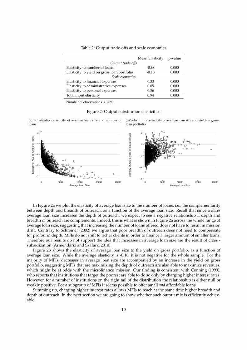
Table 2: Output trade-offs and scale economies
Mean Elasticity p-valueOutput trade-offs
Elasticity to number of loans -0.68 0.000Elasticity to yield on gross loan portfolio -0.18 0.000
Scale economiesElasticity to financial expenses 0.33 0.000Elasticity to administrative expenses 0.05 0.000Elasticity to personel expenses 0.56 0.000Total input elasticity 0.94 0.000
Number of observations is 3,890
Figure 2: Output substitution elasticities
(a) Substitution elasticity of average loan size and number ofloans
−1
−.8
−.6
−.4
−.2
Ela
sticity o
f A
LS
to
nu
mb
er
of
loa
ns
0 5000 10000 15000 20000
Average Loan Size
(b) Substitution elasticity of average loan size and yield on grossloan portfolio
−.6
−.4
−.2
0
.2
Ela
sticity o
f A
LS
to
yie
ld o
n g
ross p
ort
folio
0 5000 10000 15000 20000
Average Loan Size
In Figure 2a we plot the elasticity of average loan size to the number of loans, i.e., the complementaritybetween depth and breadth of outreach, as a function of the average loan size. Recall that since a loweraverage loan size increases the depth of outreach, we expect to see a negative relationship if depth andbreadth of outreach are complements. Indeed, this is what is shown in Figure 2a across the whole range ofaverage loan size, suggesting that increasing the number of loans offered does not have to result in missiondrift. Contrary to Schreiner (2002) we argue that poor breadth of outreach does not need to compensatefor profound depth. MFIs do not shift to richer clients in order to finance a larger amount of smaller loans.Therefore our results do not support the idea that increases in average loan size are the result of cross -subsidization (Armendáriz and Szafarz, 2010).
Figure 2b shows the elasticity of average loan size to the yield on gross portfolio, as a function ofaverage loan size. While the average elasticity is -0.18, it is not negative for the whole sample. For themajority of MFIs, decreases in average loan size are accompanied by an increase in the yield on grossportfolio, suggesting MFIs that are maximizing the depth of outreach are also able to maximize revenues,which might be at odds with the microfinance 'mission.' Our finding is consistent with Conning (1999),who reports that institutions that target the poorest are able to do so only by charging higher interest rates.However, for a number of institutions on the right tail of the distribution the relationship is either null orweakly positive. For a subgroup of MFIs it seems possible to offer small and affordable loans.
Summing up, charging higher interest rates allows MFIs to reach at the same time higher breadth anddepth of outreach. In the next section we are going to show whether such output mix is efficiently achiev-able.
10

5.2. Does the efficiency of MFIs depend on their output mix?In this section we are going to investigate the relationship between revealed preferences of the MFIs
and operational efficiency. Each MFI’s output mix is a manifestation of its preferences with respect tovarious measures of performance. Nevertheless maximizing certain dimensions of output might be morechallenging than others. For instance an institution targeting richer borrowers in an urban setting mightface stiffer competition than a rural lender, who on the other hand will incur in higher travelling costs. Inour model, efficiency does not depend only on slack, but also on the choice of output mix. We can finallyanswer the question of whether MFIs that stick to poorer clients are able to increase breadth of outreachwhile operating efficiently and whether efficiency is achieved at the cost of affordability of the loans. To findthese answers we start by looking at each single output separately and then move to pairwise combinationsof outputs.
Figure 3: Distribution of efficiency
0
1
2
3
4
De
nsity
.2 .4 .6 .8 1
Operational Efficiency
Note: mean efficiency=0.74; standard deviation = 0.13
In Figure 3 we plot the unconditional distribution of efficiency scores. The efficiency scores representthe amount of possible total output produced by an MFI given inputs and technology. An MFI with a scoreof 90% could increase its total production by 10% given its inputs. As expected the efficiency scores areskewed to the left and do not appear to be multi modals. Efficiency ranges from a minimum of 21% to amaximum of 99% with an average value of 74%. The majority of MFI operates at least at 76% efficiency.
We now focus on the correlation of a particular dimension of output with efficiency. To take into accountcountry effects, we normalized the distribution of ALS and yield on gross portfolio for each country. InFigures 4a, 4b and 4c we plot the kernel distributions of efficiency corresponding to each quartile of ourthree measures of output. In Table 7, we test the statistical significance of the differences in operationalefficiency between subsamples of the distributions. In addition to the common t-test, we use a Kruskal-Wallis (KW) rank test of the equality of population and a Kolmogorov-Smirnov (KS) test of the likeness ofthe distributions.
In Figure 4a, we show that the distribution of operational efficiency has a stronger left skew and lowervariance for lower quartiles of average loan size . The implication is that a higher proportion of MFIsoffering small loans is efficient compared to MFIs offering large loans. Hypothesis H1
0 tests whether thedistribution of efficiency for the top 50% MFIs in terms of average loan size is significantly different fromthe bottom 50%. The t test shows that the mean efficiency score for the top 50% is significantly lower thatfor the to bottom, and the KW and KS respectively confirm that the population and the distribution aresignificantly different. The hypotheses H2
0 test the differences among subsequent quartiles and betweenfirst and last quartiles, all the tests strongly reject all the H2
0 hypotheses.These results confirm both the theoretical prediction and the empirical findings of Mersland and Strøm
(2010), whom by adapting the model of Freixas and Rochet (1997) to microfinance, show that inefficient
11

Figure 4: Distribution of efficiency for different output quartiles
(a) Average loan size quartiles
0
1
2
3
4
5
kdensity te2
.2 .4 .6 .8 1
x
1st Q 2nd Q 3rd Q 4th Q
(b) Number of loans quartiles
0
2
4
6
kdensity te2
.2 .4 .6 .8 1
x
1st Q 2nd Q 3rd Q 4th Q
(c) Yield quartiles
0
1
2
3
4
kdensity te2
.2 .4 .6 .8 1
x
1st Q 2nd Q 3rd Q 4th Q
Explain what this means: allocative, technical and economic efficiency....
MFIs need to shift their portfolio towards larger loans. Interestingly the relationship between efficiencyand average loan size is the opposite of what Hermes et al. (2011) find by estimating the model with asingle output production function.
Table 3: Hypothesis tests for different output quartiles
Quartiles for: Average loan size Number of loans YieldHypothesis t-test KW KS t-test KW KS t-test KW KSH1
0 : te> ˜average − te≤ ˜average = 0 0.0000 0.0001 0.0000H2
0 : teQ1 − teQ2 = 0 0.0052 0.0024 0.0000 0.5480 0.1417 0.0000 0.0000 0.0001 0.0000H3
0 : teQ2 − teQ3 = 0 0.0000 0.0001 0.0000 0.1157 0.2732 0.0030 0.0002 0.0003 0.0000H4
0 : teQ3 − teQ4 = 0 0.0000 0.0001 0.0000 0.3689 0.7087 0.0010 0.0065 0.0039 0.0020H5
0 : teQ1 − teQ4 = 0 0.0000 0.0001 0.0000 0.0023 0.3524 0.0000 0.0000 0.0001 0.0000
Notes: KW= Kruskal-Wallis rank test; KS = Kolmogorov-Smirnov test.
Contrary to average loan size, the effect of number of loans on efficiency is not as straight forward tointerpret. In Figure 4b the kernel densities show that the distributions are more or less centred around thesame point, while the variance increases with number of loans. It is hard to identify a monotonic effecton efficiency, but we can observe higher heterogeneity of efficiency for institutions with higher breadth ofoutreach. The results of the tests confirm the ambiguity of the effect. Generally, efficiency seems to slightlydecrease with the number of loans, but this effect is not statistically significant. Economies of scale resultingfrom disbursing more loans seem to be offset by the costs of finding suitable borrowers.
Finally, we analyze the effect of yield on gross portfolio on efficiency. In Figure 4c we show that thedistribution of efficiency skews to the left for higher quartiles of yield on gross portfolio. In this casewe do not observe big differences in the variance. In Table 7 all the tests reject H5
0 , confirming that thedifference in terms of efficiency of the top and bottom half of MFIs ranked by yield on gross portfolio issignificant. Testing the differences between quartiles we see that all quartiles are significantly differentfrom the others. We conclude that efficiency monotonically increases with yield on gross portfolio. Thisresult seems to contradict Roberts (2012), but in our context it simply means that charging higher interestrates is an efficiency way to generate revenues given the cost of inputs.
In order to achieve a clearer picture, it is necessary to analyze the interaction between more than oneoutput. In Tables 4a and 4b we tabulate quartiles of average loan size against number of loans, and yieldon gross portfolio, respectively. The average efficiency score and number of observation are reported for 16combinations of quartiles per pair of outputs. We use this tabulation to analyze how differences in outputmixes influence the efficiency of the MFIs. We first look at different combinations of depth and breadth of
12

Table 4: Trade-offs between financial and social performance
(a) Average loan size and number of loans
Quartiles ALS1st 2nd 3rd 4th Total
Qua
rtile
sN
L
1st 0.770 0.763 0.743 0.727 0.748(210) (237) (207) (318) (972)
2nd 0.774 0.748 0.736 0.712 0.745(296) (271) (175) (230) (972)
3rd 0.765 0.753 0.732 0.680 0.737(260) (288) (233) (191) (972)
4th 0.775 0.769 0.729 0.664 0.730(206) (176) (357) (233) (972)
Total 0.771 0.757 0.734 0.699 0.740(972) (972) (972) (972) (3888)
(b) Average loan size and yield
Quartiles ALS1st 2nd 3rd 4th Total
Qua
rtile
sY
GP
1st 0.757 0.730 0.703 0.685 0.707(128) (152) (262) (429) (971)
2nd 0.761 0.754 0.730 0.704 0.733(167) (230) (282) (293) (972)
3rd 0.776 0.756 0.750 0.725 0.753(217) (327) (261) (167) (972)
4th 0.777 0.776 0.764 0.702 0.768(458) (263) (167) (83) (971)
Total 0.771 0.757 0.734 0.699 0.740(970) (972) (972) (972) (3886)
Can we test?
outreach and then at depth of outreach and affordability.In Table 4a we tabulate efficiency scores and number of observations (in parentheses) for quartiles of av-
erage loan size against quartiles of number of loans. From the number of observations for each combinationwe see that the two most common output mixes are either a small number of large loans (row 1, column4) or a large number of medium loans (row 4, column 3). Nevertheless the frequency of observations isquite evenly distributed, indicating strong heterogeneity in gross loan portfolio composition. Combiningthis finding with Table 1 it is clear that, when discussing mission drift, MFIs should not be divided in twogroups, as they are found in a variety of hybrid forms.
The bottom row in Figure 4b shows that efficiency is significantly lower for MFIs offering the largestloans. When average loans size is below median (first two columns), efficiency scores are always abovethe sample mean of 74%. Disbursing more or less loans has no effect on the efficiency of MFIs with deepoutreach. In the third and fourth columns we show that pretty much all MFIs with shallower depth ofoutreach operate at below average efficiency. MFIs that offer a small number of large loans score below74%. With a group average of 64%, the most inefficient MFIs are the ones offering a large number of largeloans. As shown by the rapid decrease in efficiency in column 4, inefficiencies related to mission driftbecome more serious as MFIs switch to larger loans .
We can confidently state that MFIs can achieve both depth and breadth of outreach while operating athigh levels of efficiency. If increasing loan size is the response to competition with profit oriented institu-tions (Ghosh and Tassel, 2008), it is the wrong one. MFIs offering many large loans should be experiencingeconomies of scale (Copestake, 2007), but we find no evidence of loan size improving efficiency. As a mat-ter of fact MFIs that gravitate towards a more traditional approach to banking (high breadth and low depthof outreach) are highly inefficient.
We look at the distribution of efficiency for combinations of loan size and yield on gross portfolio inTable 4b. We confirm the negative relationship between loan size and interest rates, as the most commongroups are MFIs that offer large cheap loans (row 1, column 4) and MFIs that charge high interest rateson small loans (row 4, column 1). There are only 83 observations for combinations of high yields andlarge loans. In line with Morduch (2000), this evidence shows that poorer borrowers have very low priceelasticity of demand to loans. The last column of Table 4b shows that yield on gross portfolio has a positiveeffect on efficiency. The positive effect of yields is consistently strong for the first three quartiles of ALS,but disappears for the biggest loans. MFIs offering large loans do not benefit in terms of efficiency fromraising rates. This is probably because of increased competition with the formal banking sector, MFIs arenot able to maintain efficiency while offering expensive large loans. Competition makes it more difficult tofind good borrowers, increasing both search costs and risk of the portfolio.
So it seems that the most efficient MFIs are the ones offering small, but expensive loans. This indicates
13
that depth of outreach can be achieved efficiently, but at the cost of affordability. Interestingly the top leftarea of 4b shows that a large number of MFIs are able to offer small cheap loans and still operate at higherthan average levels of efficiency.
Across the board, MFIs with larger loans are less efficient. This is at first counterintuitive and contraryto the findings of Hermes et al. (2011), but there are a number of reasons why it is plausible. Firstly, bymoving towards a different client base the experience acquired by loan officers and management will be-come less useful as well as some of the lending techniques. Secondly, competition with the formal bankingsector will increase forcing the MFIs to either cut rates or accept riskier borrowers. Finally, abandoning thepoorest borrowers will decrease the benefits that come with the microfinance status, such as lax regulatoryoversight and cheap funding.
Summing up, by analyzing the distribution of efficiency scores we show that mission drift leads toinefficiencies and especially so when MFIs try to offer a large number of large loans or charge high interestrates on them. MFIs that stick to poorer clients are more efficient. This is independent from breadth ofoutreach or the affordability of the loans offered.
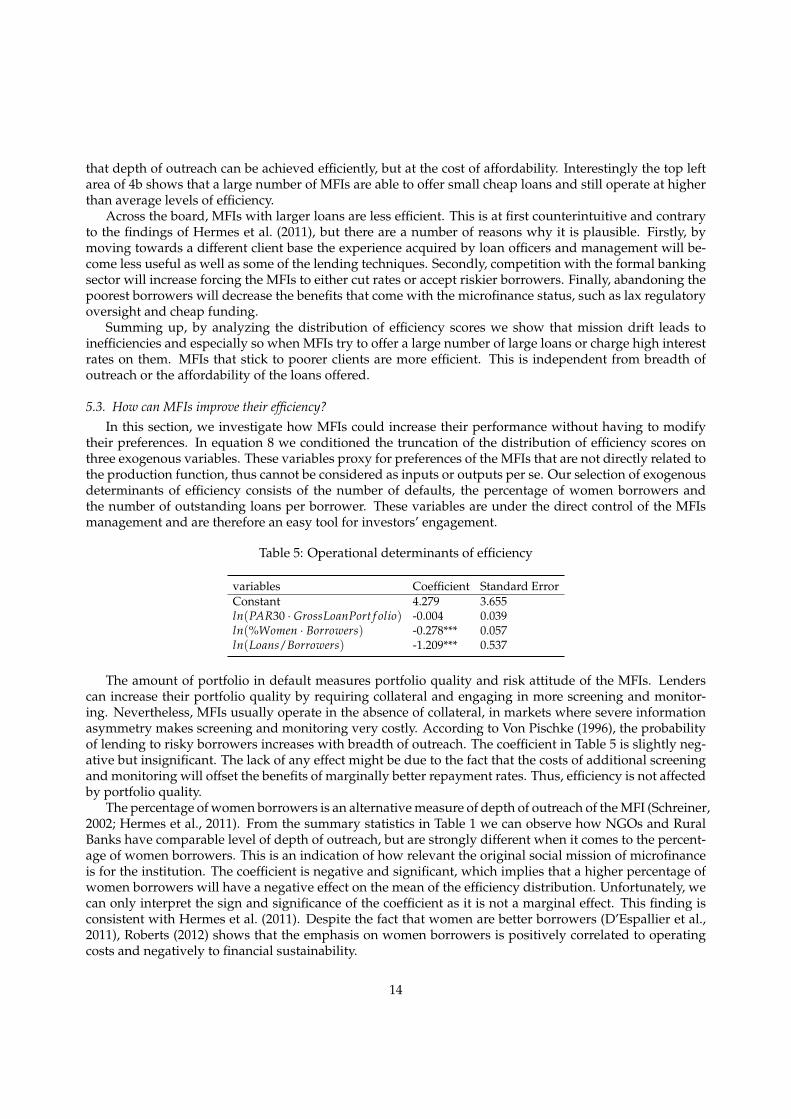
5.3. How can MFIs improve their efficiency?In this section, we investigate how MFIs could increase their performance without having to modify
their preferences. In equation 8 we conditioned the truncation of the distribution of efficiency scores onthree exogenous variables. These variables proxy for preferences of the MFIs that are not directly related tothe production function, thus cannot be considered as inputs or outputs per se. Our selection of exogenousdeterminants of efficiency consists of the number of defaults, the percentage of women borrowers andthe number of outstanding loans per borrower. These variables are under the direct control of the MFIsmanagement and are therefore an easy tool for investors’ engagement.
Table 5: Operational determinants of efficiency
variables Coefficient Standard ErrorConstant 4.279 3.655ln(PAR30 · GrossLoanPort f olio) -0.004 0.039ln(%Women · Borrowers) -0.278*** 0.057ln(Loans/Borrowers) -1.209*** 0.537
The amount of portfolio in default measures portfolio quality and risk attitude of the MFIs. Lenderscan increase their portfolio quality by requiring collateral and engaging in more screening and monitor-ing. Nevertheless, MFIs usually operate in the absence of collateral, in markets where severe informationasymmetry makes screening and monitoring very costly. According to Von Pischke (1996), the probabilityof lending to risky borrowers increases with breadth of outreach. The coefficient in Table 5 is slightly neg-ative but insignificant. The lack of any effect might be due to the fact that the costs of additional screeningand monitoring will offset the benefits of marginally better repayment rates. Thus, efficiency is not affectedby portfolio quality.
The percentage of women borrowers is an alternative measure of depth of outreach of the MFI (Schreiner,2002; Hermes et al., 2011). From the summary statistics in Table 1 we can observe how NGOs and RuralBanks have comparable level of depth of outreach, but are strongly different when it comes to the percent-age of women borrowers. This is an indication of how relevant the original social mission of microfinanceis for the institution. The coefficient is negative and significant, which implies that a higher percentage ofwomen borrowers will have a negative effect on the mean of the efficiency distribution. Unfortunately, wecan only interpret the sign and significance of the coefficient as it is not a marginal effect. This finding isconsistent with Hermes et al. (2011). Despite the fact that women are better borrowers (D’Espallier et al.,2011), Roberts (2012) shows that the emphasis on women borrowers is positively correlated to operatingcosts and negatively to financial sustainability.
14

We introduce the ratio of number of loans to number of borrowers as a rough measure of the over-lending of the MFI. Even if over-indebtedness in microfinance is a hotly debated topic (Schicks, 2010), itis a concept hard to define, let alone measure (Alam, 2012). We simply try to identify institutions that arewilling to disburse multiple loans for each borrower. We find negative and significant effect of the numberof loans per borrower on the truncation of the efficiency score distribution. Laxity in lending stronglyreduces efficiency, MFIs should be highly discouraged from allowing borrowers to enter multiple debtcontracts.
6. Conclusion
The idea behind microfinance is quite simple: to provide financial services to the poor. In reality, itsapplication is everything but simple. As a consequence of different sets of beliefs, market conditions andbusiness practices, MFIs strongly differ among each other in multiple aspects. This paper aims at bench-marking the efficiency of MFIs but avoids making any restrictions as to what the most relevant performanceindicator is. Simply put, we develop and apply a methodology that uncovers which type of MFI will makethe most out of its limited resources.
Our main methodological contribution consists in decomposing the value added of gross loan portfoliointo three factors: yield on gross portfolio, average loan size and number of loans. Each of these factorsproxies for, respectively, financial performance, profitability and outreach. Borrowing from the efficiencyliterature on banking, we utilize a stochastic frontier true fixed effect model to estimate a multi output costfunction and an efficiency score for 1146 MFIs.
From the estimation of the output frontier, we are able to extract the elasticities of average loan sizeto the other outputs and inputs. We observe that average loan size has, on average, negative elasticity tonumber of loans. The strength of the negative relationship increases with the size of the loan. MFIs canreach both depth and breadth of outreach, as they move towards better off clients, they need to increasinglydiminish the number of loans offered. Our evidence shows that mission drift does not only decrease depth,but also breadth of outreach.
Small loans are not necessarily cheap, as the negative elasticity to yield on gross portfolio shows. Onaverage, larger loans will result in lower yield on gross portfolio. We show that for a limited number ofMFIs the elasticity of average loan size to yield is zero or positive. This means that a subgroup of MFIs isable to offer small but cheap loans. Larger loans are also correlated with higher personnel and financialcosts.
The relationship between efficiency scores and outputs shows a clearly negative effect of mission drifton performance. MFIs can combine depth and breadth of outreach and maintain above average levels ofefficiency. However, efficiency quickly decreases with the size of loans and of the portfolio. Yield on grossportfolio is positively related with efficiency but high interest rates are not able to offset the inefficienciesof mission drift. Nevertheless, we observe again a sizeable group of MFIs that efficiently offer small, andmost importantly, affordable loans.
Finally we control for exogenous preferences of the MFIs such as social outreach, risk aversion andover-lending. We see that lending to women has a negative effect on efficiency. This means that a strongfocus on the women empowerment goal has to be achieved at the cost of efficiency. MFIs cannot improvetheir performance by indiscriminately lending more, in fact we show that over lending reduces efficiency.
We interpret our findings as an indication that, in terms of efficiency, transforming MFIs into bank-likefor-profit institutions might not pay off. The institutions in our sample are the most efficient when doingwhat they do best: offering relatively expensive loans to the poor. Moving towards better off clients in anattempt to reap the benefits of economies of scale, lower risk and profit oriented investments leads to aninefficient use of resources. Whether this is the effect of subsidies, lack of managerial skills or changingmarket conditions, we do not know. What we offer is a simple engagement framework that would beuseful for investors and policy makers looking at increasing the effectiveness of microfinance.
15

References
Ahlin, C., Lin, J., Maio, M., 2011. Where does microfinance flourish? microfinance institution performance in macroeconomic context.Journal of Development Economics 95 (2), 105 – 120.URL http://www.sciencedirect.com/science/article/pii/S0304387810000416
Alam, S. M., 2012. Does microcreidt creat over-indebtedness? Working paper.Armendáriz, B., Szafarz, A., 2010. On mission drift in microfinance institutions. The Handbook of Microfinance 32 (May 2009), 0–29.Battese, G. E., Coelli, T. J., July 1988. Prediction of firm-level technical efficiencies with a generalized frontier production function and
panel data. Journal of Econometrics 38 (3), 387–399.Brau, J. C., Woller, G. M., 2004. Microfinance: A comprehensive review of the existing literature. Journal of Entrepreneurial Finance
and Business Ventures 9 (1), 1–26.Conning, J., 1999. Outreach, sustainability and leverage in monitored and peer-monitored lending. Journal of Development Economics
60 (1), 51 – 77.Copestake, J., 2007. Mainstreaming microfinance: Social performance management or mission drift? World Development 35 (10), 1721
– 1738.Cuesta, R. A., Orea, L., 2002. Mergers and technical efficiency in spanish savings banks: A stochastic distance function approach.
Journal of Banking & Finance 26 (12), 2231–2247.Cull, R., Demirgüç-Kunt, A., Morduch, J., 2009. Microfinance meets the market. The Journal of Economic Perspectives 23 (1), pp.
167–192.URL http://www.jstor.org/stable/27648299
Cull, R., Demirgüç-Kunt, A., Murduch, J., 2007. Financial performance and outreach: A global analysis of leading microbanks. TheEconomic Journal 117, F107–F133.
Cull, R., Spreng, C. P., 2011. Pursuing efficiency while maintaining outreach: Bank privatization in tanzania. Journal of DevelopmentEconomics 94 (2), 254 – 261.
Debreu, G., 1951. The coefficient of resource utilization. Econometrica 19 (3), pp. 273–292.D’Espallier, B., Gu?l’rin, I., Mersland, R., 2011. Women and repayment in microfinance: A global analysis. World Development 39 (5),
758 – 772.URL http://www.sciencedirect.com/science/article/pii/S0305750X10002330
Dowla, A., Barua, D., 2006. The Poor Always Pay Back: The Grameen II Story. Kumarian Press.Färe, R., Primont, D., 1995. Multi-output Production and Duality: Theory and Applications. Kluwer Academic Publishers, Boston.Färe, R., Primont, D., 1996. The opportunity cost of duality. Journal of Productivity Analysis 7, 213–224.Farrell, M. J., 1957. The measurement of productive efficiency. Journal of the Royal Statistical Society 120, 253–281.Freixas, X., Rochet, J., 1997. Microeconomics of Banking. MIT Press, Cambridge.Fried, H., Lovell, K., Schmidt, S., 2008. The Measurement of Productive Efficiency and Productivity. Oxford University Press.Ghosh, S., Tassel, E. V., Dec. 2008. A model of mission drift in microfinance institutions. Working Papers 08003, Department of
Economics, College of Business, Florida Atlantic University.Gonzalez, A., August 2010. Microfinance synergies and trade-offs: Social versus financial performance outcomes in 2008. MIX Data
Brief 7.Greene, W., 2005. Fixed and random effects in stochastic frontier models. Journal of Productivity Analysis 23, 7–32, 10.1007/s11123-
004-8545-1.Gutiérrez-Nieto, B., Serrano-Cinca, C., Molinero, C. M., 2007. Microfinance institutions and efficiency. Omega 35 (2), 131 – 142.Hermes, N., Lensink, R., Meesters, A., 2011. Outreach and efficiency of microfinance institutions. World Development 39 (6), 938 –
948.Kodde, D. A., Palm, F. C., 1986. Wald criteria for jointly testing equality and inequality restrictions. Econometrica 54, 1243–1248.Koopmans, T. C., 1951. An analysis of production as an efficient combination of activities. In: Activity Analysis of Prodcution and
Allocation. Cowels Comminssion for Research in Economics Monograph No. 13. New York: John Wiley & Sons, Ltd.Krishnaswamy, K., 2007. Competition and multiple borrowing in the indian microfinance sector. Financial Management (September).Kumbhakar, S. C., Lovell, C. A. K., 2000. Stochastic frontier analysis. Cambridge University Press.Mersland, R., 2009. The cost of ownership in microfinance organizations. World Development 37 (2), 469 – 478.
URL http://www.sciencedirect.com/science/article/pii/S0305750X08001484Mersland, R., Strøm, R. Ø., 2009. Performance and governance in microfinance institutions. Journal of Banking & Finance 33 (4), 662
– 669.Mersland, R., Strøm, R. Ø., 2010. Microfinance mission drift? World Development 38 (1), 28 – 36.Mersland, R., Strøm, R. Ø., 2011. What drives the microfinance lending rate? Working Paper.Morduch, J., 1999a. The microfinance promise. Journal of Economic Literature 37 (4), pp. 1569–1614.Morduch, J., 1999b. The role of subsidies in microfinance: evidence from the grameen bank. Journal of Development Economics 60 (1),
229 – 248.Morduch, J., 2000. The microfinance schism. World Development 28 (4), 617 – 629.Nawaz, A., Hudon, M., Basharat, B., 2011. Does efficiency lead to lower interest rates? a new perspective from microfinance. In:
Second European Research Conference in Microfinance, Groningen, The Netherlands.Roberts, P. W., 2012. The profit orientation of microfinance institutions and effective interest rates. World Development (0), –.
URL http://www.sciencedirect.com/science/article/pii/S0305750X12001441Schicks, J., 2010. Microfinance over-indebtedness: Understanding its drivers and challenging the common myths. Working Papers
CEB 10-048, ULB – Universite Libre de Bruxelles.URL http://econpapers.repec.org/RePEc:sol:wpaper:2013/64675
16

Schreiner, M., 2002. Aspects of outreach: a framework for discussion of the social benefits of microfinance. Journal of InternationalDevelopment 14 (5), 591–603.URL http://dx.doi.org/10.1002/jid.908
Von Pischke, J. D., 1996. Measuring the trade-off between outreach and sustainability of microenterprise lenders. Journal of Interna-tional Development 8 (2), 225–239.
Appendix
17

Table 6: Output distance frontier resultsa
Variable Parameter Std.ErrorDeterministic Component of Stochastic Frontier Modelb
constant 2.85335*** (0.03966)ln(number of loans) -1.08258*** (0.01589)ln(yield) 0.03966*** (0.00751)ln(financial expenses) -0.03093*** (0.00402)ln(adminstrative expenses) 0.00622 (0.02306)ln(personnel expenses) -0.20798*** (0.02651)12 ln(number of loans)2 0.04712*** (0.00448)12 ln(yield)2 -0.02195*** (0.00173)12 ln(financial expenses)2 0.05451*** (0.00142)12 ln(adminstrative expenses)2 0.00491 (0.00613)12 ln(personnel expenses)2 0.09317*** (0.00668)ln(number of loans)×ln(yield) 0.00164*** (0.00008)ln(number of loans)×ln(financial expenses) 0.00036*** (0.00009)ln(number of loans)×ln(adminstrative expenses) 0.00055* (0.00030)ln(number of loans)×ln(personnel expenses) -0.00051 (0.00035)ln(yield)×ln(financial expenses) -0.00029*** (0.00006)ln(yield)×ln(adminstrative expenses) 0.00033** (0.00016)ln(yield)×ln(personnel expenses) 0.00019 (0.00016)ln(financial expenses)×ln(adminstrative expenses) -0.00002 (0.00017)ln(financial expenses)×ln(personnel expenses) -0.00025 (0.00017)ln(adminstrative expenses)×ln(personnel expenses) -0.00055 (0.00040)ln(number of loans)×DBank 0.00614* (0.00327)ln(number of loans)×DCooperative or credit union 0.00336 (0.00308)ln(number of loans)×DNon-bank financial institution 0.01025*** (0.00304)ln(number of loans)×DRural bank 0.00794 (0.01092)ln(yield)×DBank -0.00201 (0.00206)ln(yield)×DCooperative or credit union 0.00380** (0.00183)ln(yield)×DNon-bank financial institution -0.00226 (0.00177)ln(yield)×DRural bank -0.00669 (0.00548)ln(financial expenses)×DBank 0.00250 (0.00226)ln(financial expenses)×DCooperative or credit union -0.02378*** (0.00188)ln(financial expenses)×DNon-bank financial institution -0.00820*** (0.00138)ln(financial expenses)×DRural bank 0.00570 (0.00377)ln(adminstrative expenses)×DBank 0.00938 (0.00630)ln(adminstrative expenses)×DCooperative or credit union 0.00915** (0.00391)ln(adminstrative expenses)×DNon-bank financial institution 0.01088* (0.00556)ln(adminstrative expenses)×DRural bank 0.00786 (0.01522)ln(personnel expenses)×DBank -0.02204*** (0.00604)ln(personnel expenses)×DCooperative or credit union -0.00723* (0.00437)ln(personnel expenses)×DNon-bank financial institution -0.01131** (0.00550)ln(personnel expenses)×DRural bank -0.01556 (0.01803)
Offset [mean=µi] parameters in one sided errorc
constant 4.27916 (3.65527)portfolio share 30 days in default×gross loan portfolio 0.00411 (0.03904)% women borrows× total number of borrowers 0.27837*** (0.05773)over-lending (number of loans per borrower) 1.20890** (0.53773)
Variance parameters for compound errorλ d 3.56494*** (0.54794)σu
e 0.43976*** (0.03544)a Log likelihood function is 1660.84665; Kodde and Palm (1986) test for wrongly skewed residuals,at 95%=10.371, at 99%= 14.325. b To correct for spurious interaction terms, all variables in thetranslog have been transformed following the Frisch-Waugh theorem. c To control for possiblemulticollinearity, the variables that explain µ have been orthogonalized. d λ = σu/σv, i.e., the ratioof inefficiency and noise. e σu is the standard deviation of (untransformed) inefficiency.
18

Tabl
e7:
Effic
ienc
ytr
ade-
offs
(a)A
vera
geLo
anSi
zean
dN
umbe
rof
Loan
s
Qua
rtile
sA
vera
geLo
anSi
ze1s
t2n
d3r
d4t
hTo
tal
QuartilesN.Loans
10.
770
0.76
30.
743
0.72
70.
748
(210
)(2
37)
(207
)(3
18)
(972
)2
0.77
40.
748
0.73
60.
712
0.74
5(2
96)
(271
)(1
75)
(230
)(9
72)
30.
765
0.75
30.
732
0.68
00.
737
(260
)(2
88)
(233
)(1
91)
(972
)4
0.77
50.
769
0.72
90.
664
0.73
0(2
06)
(176
)(3
57)
(233
)(9
72)
Tota
l0.
771
0.75
70.
734
0.69
90.
740
(972
)(9
72)
(972
)(9
72)
(388
8)
(b)A
vera
geLo
anSi
zean
dY
GP
Qua
rtile
sA
vera
geLo
anSi
ze1s
t2n
d3r
d4t
hTo
tal
QuartilesYGP
10.
757
0.73
00.
703
0.68
50.
707
(128
)(1
52)
(262
)(4
29)
(971
)2
0.76
10.
754
0.73
00.
704
0.73
3(1
67)
(230
)(2
82)
(293
)(9
72)
30.
776
0.75
60.
750
0.72
50.
753
(217
)(3
27)
(261
)(1
67)
(972
)4
0.77
70.
776
0.76
40.
702
0.76
8(4
58)
(263
)(1
67)
(83)
(971
)To
tal
0.77
10.
757
0.73
40.
699
0.74
0(9
70)
(972
)(9
72)
(972
)(3
886)
(c)N
umbe
rof
Loan
san
dY
GP
Qua
rtile
sof
N.L
oans
1st
2nd
3rd
4th
Tota
l
QuartilesofYGP
10.
727
0.73
20.
703
0.65
90.
707
(270
)(2
46)
(221
)(2
35)
(972
)2
0.74
10.
747
0.72
40.
723
0.73
3(2
54)
(213
)(2
36)
(269
)(9
72)
30.
763
0.75
40.
747
0.75
20.
753
(222
)(2
34)
(265
)(2
51)
(972
)4
0.76
80.
749
0.76
90.
792
0.76
8(2
26)
(279
)(2
49)
(217
)(9
71)
Tota
l0.
748
0.74
50.
737
0.73
10.
740
(972
)(9
72)
(971
)(9
72)
(388
7)
(d)A
vera
geLo
anSi
zean
dLe
galS
tatu
s
Qua
rtile
sA
vera
geLo
anSi
ze1s
t2n
d3r
d4t
hTo
tal
Bank
0.80
30.
768
0.70
70.
728
0.74
1(3
7)(4
9)(6
0)(1
19)
(265
)C
redi
tUn
0.77
60.
766
0.76
20.
689
0.73
6(7
9)(1
05)
(121
)(2
05)
(510
)N
BFI
0.73
90.
750
0.73
50.
712
0.73
5(2
17)
(370
)(3
93)
(306
)(1
286)
NG
O0.
780
0.75
30.
721
0.66
50.
743
(627
)(3
95)
(330
)(2
68)
(162
0)O
ther
.0.
732
0.88
00.
425
0.66
9(.)
(2)
(4)
(4)
(10)
Rur
alBa
n0.
780
0.81
60.
764
0.78
00.
784
(8)
(47)
(59)
(67)
(181
)To
tal
0.77
10.
757
0.73
40.
700
0.74
1(9
68)
(968
)(9
67)
(969
)(3
872)
(e)N
umbe
rof
Loan
san
dLe
galS
tatu
s
Qua
rtile
sof
Num
ber
ofLo
ans
1st
2nd
3rd
4th
Tota
lBa
nk0.
715
0.72
90.
739
0.74
60.
740
(11)
(44)
(74)
(137
)(2
66)
Cre
ditU
n0.
763
0.77
00.
698
0.58
30.
735
(276
)(9
7)(8
6)(5
2)(5
11)
NBF
I0.
732
0.73
30.
740
0.73
30.
735
(262
)(3
46)
(348
)(3
30)
(128
6)N
GO
0.74
90.
751
0.73
70.
735
0.74
3(3
64)
(420
)(4
16)
(420
)(1
620)
Oth
er0.
640
0.73
20.
351
0.96
30.
669
(2)
(2)
(3)
(3)
(10)
Rur
alBa
n0.
764
0.77
10.
814
0.80
10.
784
(54)
(54)
(43)
(30)
(181
)To
tal
0.74
90.
746
0.73
70.
731
0.74
1(9
69)
(963
)(9
70)
(972
)(3
874)
(f)Y
ield
onG
ross
Port
folio
and
Lega
lSta
tus
Qua
rtile
sY
GP
1st
2nd
3rd
4th
Tota
lBa
nk0.
724
0.74
40.
752
0.74
80.
741
(76)
(76)
(65)
(48)
(265
)C
redi
tUn
0.71
20.
742
0.76
90.
757
0.73
5(2
26)
(139
)(8
8)(5
8)(5
11)
NBF
I0.
694
0.72
20.
757
0.75
60.
735
(284
)(3
05)
(350
)(3
46)
(128
5)N
GO
0.69
20.
731
0.74
60.
779
0.74
3(2
99)
(390
)(4
38)
(493
)(1
620)
Oth
er0.
351
0.68
60.
801
0.88
60.
669
(3)
(2)
(2)
(3)
(10)
Rur
alBa
n0.
786
0.77
70.
789
0.79
10.
784
(82)
(56)
(27)
(16)
(181
)To
tal
0.70
70.
734
0.75
40.
769
0.74
1(9
70)
(968
)(9
70)
(964
)(3
872)
19