Proceedings of the

Annual Stability Conference

Structural Stability Research Council

St. Louis, Missouri, April 16-20, 2013

Practical Design of Complex Stability Bracing Configurations

C.D. Bishop1, D.W. White

2

Abstract

The analysis and design of bracing systems for complex frame geometries can prove to be an

arduous task given current methods. AISC’s Appendix 6 from the 2010 Specification for

Structural Steel Buildings affords engineers a means for determining brace strength and stiffness

requirements, but only for the most basic cases. This paper aims to shed some light on common

aspects of certain bracing systems that lie well outside the scope of Appendix 6 as well as

explain why the corresponding structures can be unduly penalized by Specification equations

that were never derived for such use. Subsequently, a practical computational tool is proposed

that can be used to accurately assess bracing demands while removing the interpretations needed

by design engineers to “fit” their frames into the limited scope of AISC Appendix 6. The

software tool is described in detail and several benchmark cases are presented to provide

validation. Individual beams and complete framing systems are evaluated via the proposed

software and compared to refined test simulations. Finally, recommendations are articulated

governing the use of this new software as a means to accurately and safely assess bracing

demands in complex bracing configurations.

1. Introduction

Metal buildings are structures that utilize extreme weight efficiency to provide large, open floor

space at a relatively inexpensive price. Metal buildings are designed to the limits of applicable

codes and standards in order to optimize their economy while still meeting safety standards and

client objectives. Thus, locations in the standards where conservatism is abundant can unduly

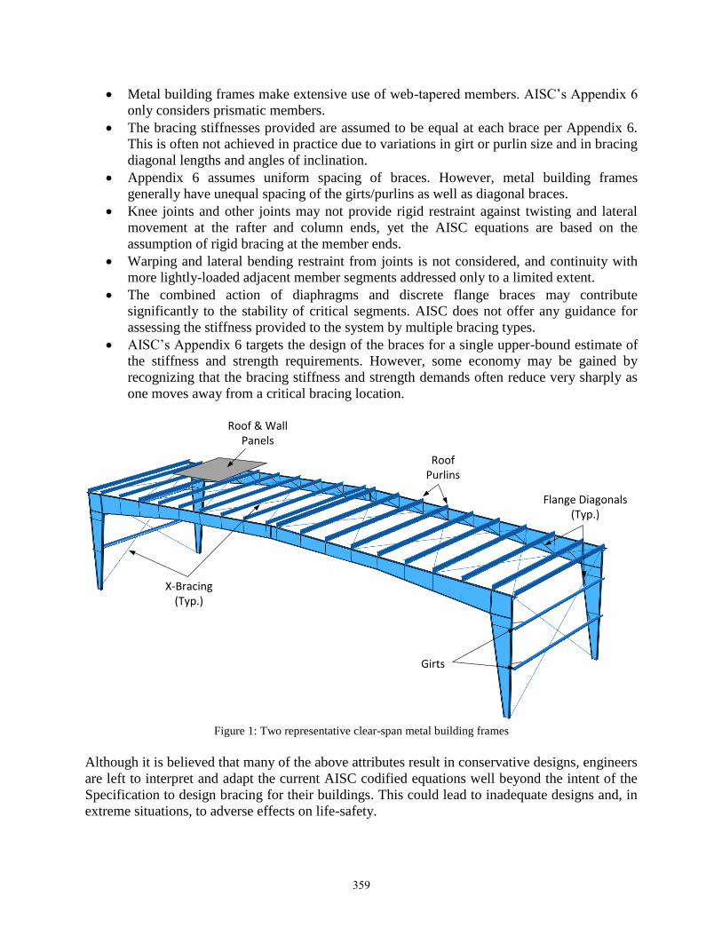
influence the steel system costs. Fig. 1 shows a rendering of a one-bay, two-frame segment of a

typical metal building.

The American Institute of Steel Construction’s Specification for Structural Steel Buildings

(2010b) Appendix 6 – “Stability Bracing for Columns and Beams” provides simplified

techniques for designing lateral and torsional braces required for stability. However, there are a

number of specific attributes of metal building systems that are outside of the scope of Appendix

6. A number of these attributes are:

1 Associate, Exponent, Inc., <cbishop@exponent.com>

2 Professor, Georgia Institute of Technology, <don.white@ce.gatech.edu>

358

Metal building frames make extensive use of web-tapered members. AISC’s Appendix 6

only considers prismatic members.

The bracing stiffnesses provided are assumed to be equal at each brace per Appendix 6.

This is often not achieved in practice due to variations in girt or purlin size and in bracing

diagonal lengths and angles of inclination.

Appendix 6 assumes uniform spacing of braces. However, metal building frames

generally have unequal spacing of the girts/purlins as well as diagonal braces.

Knee joints and other joints may not provide rigid restraint against twisting and lateral

movement at the rafter and column ends, yet the AISC equations are based on the

assumption of rigid bracing at the member ends.

Warping and lateral bending restraint from joints is not considered, and continuity with

more lightly-loaded adjacent member segments addressed only to a limited extent.

The combined action of diaphragms and discrete flange braces may contribute

significantly to the stability of critical segments. AISC does not offer any guidance for

assessing the stiffness provided to the system by multiple bracing types.

AISC’s Appendix 6 targets the design of the braces for a single upper-bound estimate of

the stiffness and strength requirements. However, some economy may be gained by

recognizing that the bracing stiffness and strength demands often reduce very sharply as

one moves away from a critical bracing location.

Figure 1: Two representative clear-span metal building frames

Although it is believed that many of the above attributes result in conservative designs, engineers

are left to interpret and adapt the current AISC codified equations well beyond the intent of the

Specification to design bracing for their buildings. This could lead to inadequate designs and, in

extreme situations, to adverse effects on life-safety.

X-Bracing (Typ.)

Roof Purlins

Flange Diagonals (Typ.)

Girts

Roof & Wall Panels

359

Lastly, the AISC Specification Appendix 6 provisions estimate the maximum brace strength and

stiffness demands throughout a given member generally assuming constant brace spacing and

constant brace stiffness. However, this method is not practical for members with a large number

of brace points along their length. When considering the sample frames shown in Fig. 1, several

questions may come to mind:

1. Are the bracing requirements at the knee influenced significantly by the loading, cross-

section geometry or arrangement of bracing at the ridge?

2. What constitutes a support point? That is, at what locations is the out-of-plane movement

of the frame sufficiently restrained? Do any locations of attachment of the panel or rod

bracing provide this restraint?

3. How do the rafters interact with the columns and vice versa with respect to the bracing

demands?

In general, all the members and their bracing components work together as a system in structural

frames such as that shown in Fig. 1. Therefore, the central question addressed in this paper is:

What are the overall physical bracing strength and stiffness demands required to develop the

required strength of the structure?

2. Toward a Comprehensive Bracing Tool

Due to the complex and interrelated nature of the attributes discussed above, this paper focuses

on the development of a comprehensive computational bracing analysis tool for the direct

assessment of stability bracing requirements. Any such tool would need to be robust enough to

include consideration of all of the above items, yet remain simple enough for use in practice. The

following is a summary of why such an analysis tool is required for bracing design in metal

building structures.

The current AISC Specification equations for stability bracing are derived from solutions of the

elastic eigenvalue buckling of members and their bracing systems. However, the nominal

flexural strength of columns and rafters of metal building frames is usually controlled by

inelastic lateral-torsional buckling, once the frames are in their final constructed configuration.

The Appendix 6 equations address this (for LRFD of beam bracing) by a three-staged

approximation:

1) Replacing the elastic critical moment Mcr by the design strength Mn, thus implicitly

estimating the bracing demands, as the elastic or inelastic strength limit Mn is

approached, by the normalized behavior of the system as the elastic buckling load is

approached, then

2) Replacing Mn by the required strength Mu, which is generally smaller than Mn for a

properly designed beam. This is based on the implicit approximation that the partial

bracing stiffness demands can be estimated conservatively by this manipulation.

Furthermore, where applicable (i.e., only for nodal lateral beam bracing), the

Specification allows the use of Lq in place of Lb, where Lq is taken as the unbraced length

that reduces Mn to Mu. This completes the approximations in the AISC bracing

equations for the partial bracing stiffness demands.

360

3) Lastly, for cases involving partial bracing, the AISC equations assume that the strength

requirement for partial bracing is estimated sufficiently simply by using Mu in the

equations for the strength requirement (along with the use of Lq). This appears to be an

acceptable approximation for practical partial bracing cases approaching full bracing, but

it can break down for weak partial bracing, where the amplification of the initial

imperfection displacements may become substantial.

The various factors listed above may render the bracing system design over-conservative by as

much as 10x that required based on inelastic load-deflection solutions when applied to typical

metal building frames (Sharma 2010). A portion of the conservatism observed by Sharma (2010)

may be due to the approximations detailed above; however, a larger portion is likely due to the

fact that many of the metal building system attributes are not addressed explicitly by the AISC

equations.

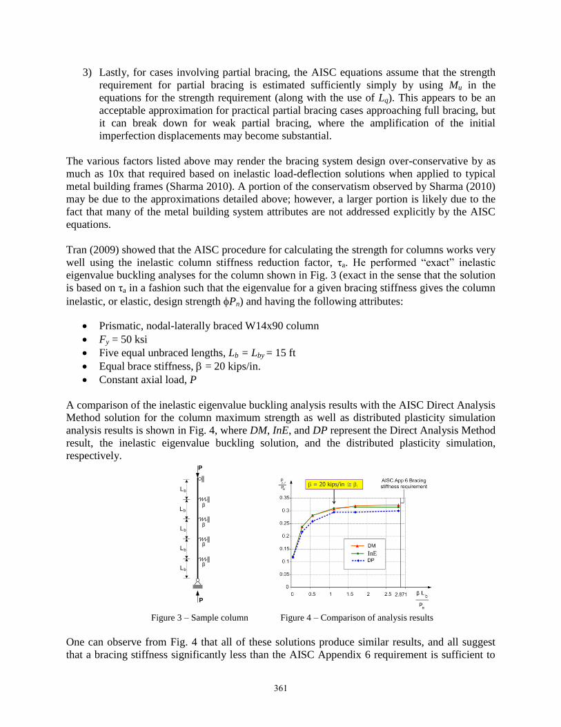
Tran (2009) showed that the AISC procedure for calculating the strength for columns works very

well using the inelastic column stiffness reduction factor, τa. He performed “exact” inelastic

eigenvalue buckling analyses for the column shown in Fig. 3 (exact in the sense that the solution

is based on τa in a fashion such that the eigenvalue for a given bracing stiffness gives the column

inelastic, or elastic, design strength Pn) and having the following attributes:

Prismatic, nodal-laterally braced W14x90 column

Fy = 50 ksi

Five equal unbraced lengths, Lb = Lby = 15 ft

Equal brace stiffness, = 20 kips/in.

Constant axial load, P

A comparison of the inelastic eigenvalue buckling analysis results with the AISC Direct Analysis

Method solution for the column maximum strength as well as distributed plasticity simulation

analysis results is shown in Fig. 4, where DM, InE, and DP represent the Direct Analysis Method

result, the inelastic eigenvalue buckling solution, and the distributed plasticity simulation,

respectively.

Figure 3 – Sample column Figure 4 – Comparison of analysis results

One can observe from Fig. 4 that all of these solutions produce similar results, and all suggest

that a bracing stiffness significantly less than the AISC Appendix 6 requirement is sufficient to

P

Lb

Lb

Lb

Lb

Lb

β

β

β

β

P

InE

361

develop the full-bracing resistance for this column example. Tran (2009) showed that for this

problem, the use of a nodal bracing stiffness equal to the ideal bracing stiffness, labeled as i =

20 kips/inch in Fig. 4, resulted in brace strength demands only slightly larger than 2 % in

distributed plasticity simulation studies.

Although the solution by the DM is reasonably accurate, this method (often thought of as a

reasonable approximation of the results from a rigorous distributed plasticity simulation analysis

or a physical test, and thus providing the best design assessment for stability requirements) may

not be a feasible option for assessing stability bracing demands in problems like this due to the

following fact: With the DM, as well as with the simulation analysis, an appropriate magnitude

and pattern of the initial geometric imperfections must be imposed on the member to estimate the

maximum strength demand on a given brace in question. This means that one must consider

geometric imperfections in a manner similar to the way that load combinations are considered in

general strength design. For each specific brace, an imperfection needs to be identified that

produces the maximum demand on that brace. Although procedures have been identified by

Sharma (2010) and others to determine the “critical” imperfection for a given brace, these

procedures are relatively complex and in general may require a number of trials to truly identify

the critical imperfection. Of equal importance is that these procedures would generally need to

be executed for each brace within the structural system. This level of effort can be tolerated for

research studies; however, it is not practical for ordinary design.

In contrast, the “exact” inelastic eigenvalue buckling analysis gives similar results to the DM or

DP solutions with much less computational effort. However, one should note that an eigenvalue

buckling analysis only provides the designer with an estimate of the required bracing stiffness

and the overall system strength. As has been discussed extensively (see, Yura (2001) for

example), to be effective, a brace must provide sufficient stiffness and strength to resist the loads

imparted to it by the braced member. Fortunately, Sharma (2010) and Tran (2009) have shown

through numerous finite element simulations that the brace force is usually in the range of 2 to

3% of the effective flange force for nodal bracing cases approaching full bracing. In fact, 2% is

often enough to allow the frame to reach 95% of its rigidly-braced capacity. Therefore, one can

combine the brace stiffness requirement from an inelastic eigenvalue buckling analysis with say,

a 2 to 4% brace strength rule (for frames not specifically required to sustain large inelastic

cyclical loadings) for a complete determination of the bracing requirements.

Creation of a new computational bracing analysis tool is needed because no current structural

analysis software provides the specific necessary elements or combination of analysis methods to

produce the type of solutions illustrated in Fig. 4 for general member and/or frame geometries

and general bracing arrangements. The targeted bracing analysis tool must be able to address

such aspects as warping and out-of-plane bending restraint, roof and wall “shear panel” (i.e.,

relative) bracing combined with nodal torsional bracing, combined effects of axial and flexural

loading, unequal brace spacing, web taper, and steps in the cross-section geometry. The

computational tool needs to be able to solve for the in-plane elastic and/or inelastic state of a

member or frame at a given design load level, or at an envelope of all the maximum internal

forces based on a range of design loadings, and then determine the ideal bracing stiffness

demands (i.e., the required ideal bracing stiffness) to sufficiently stabilize the structure in this

elastic/inelastic state.

362

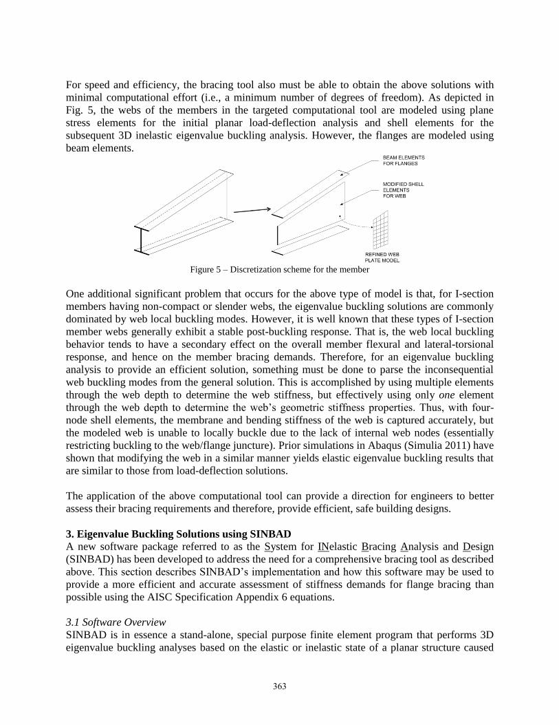
For speed and efficiency, the bracing tool also must be able to obtain the above solutions with

minimal computational effort (i.e., a minimum number of degrees of freedom). As depicted in

Fig. 5, the webs of the members in the targeted computational tool are modeled using plane

stress elements for the initial planar load-deflection analysis and shell elements for the

subsequent 3D inelastic eigenvalue buckling analysis. However, the flanges are modeled using

beam elements.

Figure 5 – Discretization scheme for the member

One additional significant problem that occurs for the above type of model is that, for I-section

members having non-compact or slender webs, the eigenvalue buckling solutions are commonly

dominated by web local buckling modes. However, it is well known that these types of I-section

member webs generally exhibit a stable post-buckling response. That is, the web local buckling

behavior tends to have a secondary effect on the overall member flexural and lateral-torsional

response, and hence on the member bracing demands. Therefore, for an eigenvalue buckling

analysis to provide an efficient solution, something must be done to parse the inconsequential

web buckling modes from the general solution. This is accomplished by using multiple elements

through the web depth to determine the web stiffness, but effectively using only one element

through the web depth to determine the web’s geometric stiffness properties. Thus, with four-

node shell elements, the membrane and bending stiffness of the web is captured accurately, but

the modeled web is unable to locally buckle due to the lack of internal web nodes (essentially

restricting buckling to the web/flange juncture). Prior simulations in Abaqus (Simulia 2011) have

shown that modifying the web in a similar manner yields elastic eigenvalue buckling results that

are similar to those from load-deflection solutions.

The application of the above computational tool can provide a direction for engineers to better

assess their bracing requirements and therefore, provide efficient, safe building designs.

3. Eigenvalue Buckling Solutions using SINBAD

A new software package referred to as the System for INelastic Bracing Analysis and Design

(SINBAD) has been developed to address the need for a comprehensive bracing tool as described

above. This section describes SINBAD’s implementation and how this software may be used to

provide a more efficient and accurate assessment of stiffness demands for flange bracing than

possible using the AISC Specification Appendix 6 equations.

3.1 Software Overview

SINBAD is in essence a stand-alone, special purpose finite element program that performs 3D

eigenvalue buckling analyses based on the elastic or inelastic state of a planar structure caused

363

by the application of in-plane loads. The solutions from SINBAD may be used to either

determine member or framing system out-of-plane buckling capacities or to determine ideal

stiffnesses of the corresponding out-of-plane bracing system. The in-plane inelastic analysis

capabilities of SINBAD involve a complete spread of plasticity (or plastic zone) analysis of the

structure including any appropriate in-plane geometric imperfections as well as specified

member nominal residual stresses. SINBAD is written in Matlab (MathWorks 2011) and

includes both an analysis engine and a graphical user interface (GUI).

SINBAD has two distinct modules: members and frames. The members module is used

exclusively to assess the bracing requirements for individual members. For example, one can

analyze a given physical beam or column segment for analysis as an isolated member. That is,

the member module is only useful to model one member. In the frame module, SINBAD

provides the ability to assess the bracing requirements for an entire framing system. The frame

can have any generalized geometry but must have no more than two exterior columns and two

rafters (one on each side of a ridge location). The input to SINBAD may be accomplished either

by a set of Microsoft Excel worksheet forms or via a general application program interface.

3.2 FEA Modeling

The following sub-sections describe some of the individual components that comprise SINBAD.

The inelastic buckling analysis solutions in SINBAD are conducted generally in two steps:

1. The 2D (planar) elastic/inelastic state of the structure is calculated given a prescribed

loading condition, and

2. A 3D eigenvalue buckling analysis is performed based on the stress state determined in

Step 1.

By limiting the stress determination to a planar solution, significant analysis time savings are

realized relative to the requirements for a general 3D simulation such as that conducted in

Abaqus. After the state of stress is determined, the program must “upgrade” the model to its 3D

counterpart in order to assess the out-of-plane stability of the system in question. Details about

how this solution is achieved efficiently are provided in the following sections.

3.2.1 Flange Elements

All flanges and stiffeners are modeled in SINBAD using 2-node cubic Hermitian beam elements

with one additional internal axial degree of freedom, providing for a linear variation in the

interpolated strains along the member length for both axial and bending deformations (White

1985). For the planar solution, there are a total of 7 degrees of freedom: two translations and one

out-of-plane rotation at each end plus an additional axial degree of freedom at the middle of the

element. The interior axial degree of freedom is removed via static condensation (see McGuire,

et al. 2000, for example) to leave a total of 6 global degrees of freedom. For the 3D model, a

total of 13 degrees of freedom are used for the beam element: three translations and three

rotations at the member ends plus one additional axial degree of freedom at the middle of the

element. Again, static condensation is performed to render 12 global degrees of freedom.

To track the spread of plasticity through the beam element, White (1985) proposed a fiber model

that subdivides each element into a predefined grid. 12 fibers are used through half the width of

the flange (bf/2) and 2 fibers through the thickness of the flange (tf). It is only necessary to model

364

the grid over one-half of the flange width since the planar solution is symmetric about the plane

of the structure. Tracking the spread of yielding throughout the element is performed on an “as

needed” basis. That is, the fiber grid is only created when the global element has detected

yielding. This reduces the memory requirements and substantially increases the computation

speed. For brevity, the reader is referred to White (1985) for a further discussion and step-by-

step implementation of this second-order inelastic element.

3.2.2 Web Elements

The web shell elements are created through the combination of a QM6 element for plane stress

and a PBMITC element for plate bending.

The QM6 is created by starting with the general four-node isoparametric quadrilateral element

(Q4) and then making the following two modifications:

1. To prevent shear locking, bending deformation modes are included by adding

incompatible modes to the element’s displacement field. This reduces the element’s

tendency to be overly stiff when displaying bending-type deformations and creates the

commonly known Q6 element (Cook 2002).

2. The determinant of the Jacobian is evaluated only at the middle of the element. This

modification allows the Q6 element to represent constant stress (or shear) states for

shapes other than rectangles and thus, the element is able to pass all patch tests and is

renamed the QM6 element.

The PBMITC element is a four-node mixed interpolation of tensorial components element

originally derived by Bathe and Dvorkin (1985). The inclusion of the mixed interpolation

removes shear locking of the element while avoiding spurious zero-energy modes.

After combination of the QM6 and the PBMITC elements, an additional “null” drilling degree of

freedom is included at nodes that are attached to the beam elements to accommodate the three

rotational nodal dofs of the 3D frame element; only two rotational dofs are required at the other

shell nodes.

An important aspect of SINBAD focuses on a formulation of the geometric stiffness for the web

shell finite elements such that web local buckling modes are not considered in the 3D eigenvalue

buckling solutions. As discussed in Section 2, due to the nature of the web being stable in its

post-buckled state plus the fact that the brace demands are usually driven by lateral bending of

the flanges, removing the local web modes provides a substantial improvement in the efficiency

in the solution algorithm while focusing on solving for the member or frame out-of-plane

buckling. As shown in Fig. 6, the following solution scheme is proposed to eliminate the

handling of local web buckling modes:

1. Determine the stress at the Gauss points within each web “sub-element” from the in-

plane analysis (in Fig. 6, 16 Gauss points, each with three stress measures).

2. Use Gauss quadrature within each sub-element to integrate over the volume of each

“super-element,” composed of all the sub-elements through the depth of the web, to

obtain a single geometric stiffness for each web super-element.

365

WEB “SUB-

ELEMENT” (TYP.)

WEB “SUPER-

ELEMENT”

GAUSS POINT

(TYP.)

Figure 6: Web sub-elements for calculation of the geometric stiffness matrix

This process ultimately arrives at a solution that approximates the effect of “condensing” out the

geometric stiffness terms associated with the internal web sub-element nodal dofs and leaving

just the corner nodes of the “super-element” for the global 3D buckling solution. The global

buckling solution is effectively limited to the movements associated only with the “super-

element” corner nodes.

3.2.3 Bracing Elements

There are three distinct types of bracing (as termed by AISC 2010b), and any general

combination of these types is addressed by SINBAD:

1. Nodal (discrete grounded) bracing

2. Relative (shear panel) bracing

3. Nodal torsional bracing

When implementing nodal bracing, SINBAD simply includes a grounded spring stiffness

directly in the global stiffness matrix at the out-of-plane translational degree of freedom

associated with the brace location. For relative bracing, SINBAD models the bracing as a “shear”

spring by incorporating a basic 2x2 element stiffness matrix that resists the relative out-of-plane

movement of two connected points. Lastly, nodal torsional bracing is modeled in a manner

similar to the nodal relative bracing with the added step that the program must first divide the

user input torsional bracing stiffness (in units of force x length/radian) by the web-depth squared

to determine an equivalent shear spring stiffness. It is also important to note here that these

spring elements are only required for the out-of-plane buckling solution. Since the 2D, nonlinear

solution only deals with deflections in-plane, the degrees of freedom associated with the out-of-

plane movement at the braces (or springs) is not activated and thus, not required in the planar

global stiffness matrix.

366

3.3 Material Description

The material model employed in SINBAD considers that the steel remains elastic at modulus E

up to the yield stress Fy (and yield strain εy), exhibits a yield plateau with a minimal hardening at

a small modulus Et (used for numerical purposes) from εy up to εst = 10εy, and then experiences

strain hardening at Est above εst. The tangent modulus is taken E/100 within the yield plateau of

the material stress strain curve. It should be noted that this stiffness value is approximately equal

to the bounding stiffness exhibited by typical structural steels upon cyclic loading of the material

(see White 1988, for example). SINBAD uses E = 29,000 ksi for the steel elastic modulus and Est

= 900 ksi for the steel strain-hardening modulus.

3.4 Residual Stresses

Fig. 7 shows the residual stress pattern employed in SINBAD. This is selected as a nominal

residual stress distribution that provides a close representation of the column inelastic flexural

and beam inelastic lateral-torsional buckling strength curves from the AISC (2010b)

Specification. The flange residual stress distribution is the same as that recommended by ECCS

(1983) for rolled I-section beam members with h/bf > 1.2, and the web residual compression is

representative of that observed in welded I-section members with noncompact and slender webs

(Avent and Wells, 1979; Nethercot, 1974). White (2008) discusses a large set of experimental

data upon which the AISC lateral-torsional and flange local buckling strength curves are based,

and shows that the influence of the type of I-section (rolled or welded) on the strengths is of

minor significance given this data. This justifies the use of the single beam lateral-torsional

buckling or column flexural buckling strength curves in AISC (no distinction in the resistances

for rolled or welded cross-sections), and thus also may be used as a justification for the use of a

single nominal residual stress pattern for the flanges as shown in Fig. 7. For I-section members

with noncompact or slender webs, an interesting result is that the web typically cannot sustain

substantial stresses in uniform axial compression over most of its depth without experiencing

local buckling. Therefore, the maximum uniform web compressive residual stress is taken as the

smaller value of 0.1Fy or the elastic local buckling stress of the web under uniform axial

compression, Fcrw, assuming simply-supported edge conditions. The web residual tension is

modeled over a depth of h/8 at the top and bottom of the web such that the residual stress pattern

in the web is self-equilibrating. Of course, the flange residual stresses shown in Fig. 7 are also

self-equilibrating. For web-tapered members, the above web residual stresses are calculated at

the mid-length of each tapered member. This is a simplification of the potential web residual

stresses in a physical tapered member with a noncompact or slender web, which may in fact vary

along the member length as a function of the web buckling resistance to the longitudinal residual

compression.

4. Member Module

This section highlights the use of SINBAD to assess member bracing stiffness requirements.

The results from SINBAD are compared to AISC (2010b) and to rigorous load-deflection

simulations using Abaqus (Simulia 2011). The plots presented show representative member

strength versus bracing stiffness results, which are commonly referred to as a “knuckle curves”.

For these types of graphs, one generally plots the bracing stiffness in kips/inch for relative

bracing and kips x inch/radian for torsional bracing on the abscissa and some measurement of the

member strength on the ordinate (Mmax/(My) for these plots). Knuckle curves generally exhibit a

region that may be referred to as the “plateau.” The plateau is the portion of the knuckle curve

367

where the strength of the fully-braced member has been reached and further increases in the

bracing stiffness do not provide any significant additional member capacity.

compression

tension

0.3Fy

0.3Fy 0.3Fy

compressiontension

0.3Fy

0.3Fy

h/8

3h/4

h/8

min(0.1Fy,Fcrw)

Figure 7: Residual stress pattern for flanges (left) and web (right)

4.1 Qualification of Simulations Using Abaqus

As mentioned above, Abaqus (Simulia 2011) is selected as the benchmark to assess SINBAD’s

ability to predict accurate bracing stiffness demands. Due to the complexity of the stability

bracing systems in metal building frames combined with the wide range of factors that can influ-

ence the bracing response (as discussed in the introduction), a large number of member and

frame tests is needed to develop meaningful (and generalizable) bracing data. Simulation pro-

vides the only economical approach to generate this data. Furthermore, stability bracing force de-

mands generally are sensitive to the pattern of the geometric imperfections. Therefore, evaluating

maximum required bracing forces for design generally necessitates the calculation of the critical

geometric imperfection. Forcing initial geometric imperfections on physical members that cause

the largest demands on the bracing system in an experimental test may prove difficult. However,

critical geometric imperfections can be generated with relative ease for simulation studies. Vali-

dation of simulation methods against experimental test data for members on which detailed phys-

ical geometric imperfection and residual stress measurements have been documented provides an

important validation of the simulation models. These simulation models can then be applied to

provide detailed assessment of the true maximum design bracing strength and stiffness demands.

The Abaqus simulations discussed in this paper use the same residual stress pattern as described

for SINBAD. Also, since load-deflection analyses are driven by initial imperfections, patterns of

initial imperfections were selected within allowable erection tolerances specified in AISC’s Code

of Standard Practice (2010a) and the Metal Building Systems Manual (MBMA 2006). The nature

of selecting and implementing the necessary initial imperfections is beyond the scope of this

paper. The reader is referred to Tran (2009), Sharma (2010), Kim (2010), and Bishop (2013) for

a more complete discussion of the process necessary to select the critical initial imperfections.

368

4.2 Example 1: W16x26 with Relative Bracing under Uniform Moment

Fig. 8 shows the results for a W16x26 loaded under uniform moment with three equally-spaced

unbraced lengths, each with Lb = 4 ft. There are four relative braces, all of equal stiffness, along

the compression flange of the member. The above unbraced length places this section in the

inelastic buckling region for this cross-section profile. All the end conditions for these example

cases are ideally simply-supported, flexurally and torsionally. That is, hinges and rollers are

assumed for the in-plane end conditions and “fork” end conditions (out-of-plane flexure and

warping of the flanges unrestrained) are assumed for the out-of-plane buckling analysis.

Figure 8: Example 1; W16x26, uniform moment, 4 relative braces, Lb = 4 ft

In Fig. 8 legend (and all subsequent legends in this section), the following nomenclature is used:

“βAISC” is the stiffness requirement obtained from AISC Appendix 6 for either relative

bracing via Equation 1 or torsional bracing via Equation 2. Note that these equations have

been rewritten to incorporate a refined estimate of the bracing stiffness based on the

Commentary to Appendix 6 (AISC 2010b).

dtR

b

orbr CC

L

hMβ

)/(2 (1, AISC A-6-6)

.

1β 10ψ

r r

2 b o b o T

T o tT

ef eff b T

M MC h C h (n )

h CP L n

(2, AISC A-6-11)

where = 1/ = 1/0.75 = 1.33 for LRFD, Lb = spacing between the brace points, assumed

constant in the development of Eq. 2, Mr = required flexural strength in the beam from the

LRFD load combinations, ho = distance between flange centroids, Cb = equivalent uniform

moment factor for a given unbraced length, based on flange stresses for non-prismatic

members (ad hoc extension), Cd = double curvature factor, CtR = flange load height factor for

0.50.55

0.60.65

0.70.75

0.80.85

0.90.95

11.05

1.11.15

0 1 2 3 4 5 6 7 8

Mm

ax/(

My)

βR (kip/in.)

Beta_AISC

Simulation

SINBAD

Beta_Req

βAISC

βReq

369

relative bracing, CtT = flange load height factor for torsional bracing, nT = number of

intermediate nodal torsional brace points within the member length between the rigid “end”

brace locations, where both twisting and lateral movement of the beam are prevented, Pef.eff

= effective flange buckling load = 2EIf.eff / Lb

2, E = steel modulus of elasticity = 29,000 ksi,

If.eff = Iyc for doubly-symmetric sections or (ytyc I

c

tI )/2

for singly-symmetric sections, c =

distance between cross section centroid and compression flange centroid, t = distance

between cross-section centroid and tension flange centroid, Iyc = lateral moment of inertia of

the compression flange, and Iyt = lateral moment of inertia of the tension flange.

“Simulation” refers to the member maximum strength obtained from the test simulations

conducted using Abaqus.

“SINBAD” refers to the member inelastic, out-of-plane buckling strength from SINBAD

based on a given ideal bracing stiffness. In this paper, ideal bracing stiffness is defined as

the stiffness required to brace a perfectly straight member such that a particular out-of-

plane buckling resistance is achieved. Due to the fact that physical columns and beams

have inherent geometric imperfections, immediately upon application of load, the initial

deflections present in the member begin to be amplified (Timoshenko and Gere 1961).

This amplification of the initial imperfections impacts the brace force demands, since

brace point displacement times the bracing stiffness (assumed to remain elastic) generates

the brace forces. Therefore, one finds that while theoretically it is possible to provide the

ideal stiffness for a given member assuming the member is perfectly straight, practically,

one must often provide some multiple of that value in an effort to keep the brace forces

(and brace strength design requirements) manageable for real members where initial

imperfections are unavoidable. It is common in the literature to use a multiple of 2/

where the resistance factor = 0.75 on the ideal bracing stiffness in order to limit the

amplification of brace point movement and the resulting brace forces (Yura 2001).

“βReq” is a “SINBAD” generated curve in which the abscissa is scaled by the larger of 3/

times the result determined from an elastic eigenvalue buckling analysis or 2/ times the

result determined from an inelastic eigenvalue buckling analysis at a given strength level.

The coefficients 2/ and 3/ are needed as discussed above and to parallel the approach

taken in AISC Appendix 6 of scaling the ideal bracing stiffness to determine a required

design bracing stiffness, where is the resistance factor taken equal to 0.75 (AISC

2010b). The justification of this curve is detailed below.

The first item of note from Fig. 8 is the difference in the strength of the member reached when

full bracing is provided; i.e., the plateau strength comparisons from the SINBAD, simulation,

and AISC results. In this case, SINBAD reaches a strength limit at Mmax/(My) = 0.96, Abaqus

suggests Mmax/(My) = 1.05 and the AISC equations suggest Mmax/(My) = 1.1. The following is a

discussion on why this variance in the capacity for rigid bracing occurs.

The main difference between the results from a general eigenvalue buckling analysis (SINBAD

in this case) and the AISC Specification is due to the lateral movement of the compression

flange. The inelastic eigenvalue buckling analysis is based on the state of the structure associated

370

with in-plane deformations. That is, the member is assumed to displace solely in-plane until the

critical buckling load is reached. At this point, the member then displaces laterally out-of-plane

an undetermined amount. Conversely, the AISC design curves are a fit to experimental data.

Therefore, due to the imperfect nature of the initial geometry in real test specimens, lateral

movement of the compression flange initiates immediately with the onset of load. This lateral

movement increases as the load increases, exacerbating the compression on one side of the

compression flange and relieving compression on the other. Therefore, a potentially higher load

may be reached in certain cases in experimental tests when compared to an eigenvalue buckling

analysis. The ASCE-WRC Plastic Design Guide (ASCE 1971) discusses this phenomenon in

detail and documents these observations for compact-web sections with relatively close brace

spacing subjected to uniform moment.

One key source of differences between the results from the simulation results from Abaqus and

the AISC Specification is due to the initial conditions; i.e., the magnitude and location of initial

imperfections and the magnitude and distribution of residual stresses. The residual stresses, as

discussed in Part 3, are representative of those determined from Avent and Wells (1979) and

Nethercot (1974). However, many experiments on which the design curves are based did not

have their residual stresses recorded. Also, as was alluded to earlier yet the details were omitted,

the initial imperfections determination may not be as unfavorable as those employed in the

simulation. Due to the current erection tolerances specified by AISC (2010a) and MBMA

(2006), it is common to take some combination of these tolerances to create a “worst case

scenario” for the pattern of initial imperfections. Where one might suggest that a procedure that

invokes the worst possible pattern is overly conservative, it may be difficult to justify a more

unconservative pattern. Statistically, it is improbable for an experimental specimen to have the

worst case imperfection pattern as well as the worst-case residual stress pattern. Therefore, the

imperfections and residual stresses used in the simulation will often be higher than those realized

in experiments, leading to a solution predicting less capacity. In addition, for the uniform

inelastic bending case, the representation of the member response as a continuum is a clear

idealization of the physical response generally observed from experiments (ASCE 1971).

Next, one may compare the stiffness suggested from βReq versus that suggested by βAISC. One of

the reasons the AISC prediction is high relative to the results from SINBAD (larger bracing

stiffness required to achieve a given beam moment resistance) is because the AISC equation for

the relative bracing stiffness requirement (Eq. 1) ignores the contribution of the member to the

resistance of brace point movement (Yura 2001). That is, all out-of-plane displacements must be

resisted by the provided bracing, with no consideration of the member’s own inherent ability to

resist brace point movement. The two plots from SINBAD (including both the ideal stiffness and

the scaled ideal stiffness) consider the member’s ability to resist out-of-plane brace movement.

As introduced earlier, βReq is produced by combining the larger of 3/0.75 times the ideal elastic

bracing requirement from SINBAD or 2/0.75 times the ideal inelastic bracing requirement from

SINBAD. (For clarity, the bracing stiffness required from an elastic eigenvalue buckling analysis

using SINBAD is not shown on the plot.) βReq is a reasonable metric since it incorporates values

of bracing stiffness that would buckle the member elastically (using 3/0.75 times the ideal

stiffness), yet reduces this scaling of the stiffness requirements to 2/0.75 as the member begins to

yield. Also, it should be noted that βReq has been calibrated to a large set of results. Therefore, the

371

conservatism realized in this specific case is not necessarily representative of the level of

conservatism in other cases.

4.3 Example 2: W16x26 with Torsional Bracing under Uniform Moment

Example 2 is also a W16x26 loaded with uniform moment. However, the member now has 3

interior torsional braces, all with equal stiffness, in lieu of relative bracing. Again, Lb = 4 ft and

the member is classified in the inelastic lateral-torsional buckling region. The results for

Example 2 are shown in Fig. 9.

Figure 9: Example 2; W16x26, uniform moment, 3 torsional braces, Lb = 4 ft

When looking at the bracing requirement for a particular load level, say at Mmax/(My) = 0.65, the

Abaqus simulation suggests that a bracing requirement of 450 kip x in./rad is required at each

brace. The prediction for the ideal bracing requirement from SINBAD is closer to 200 kip x

in./rad. However, to keep brace point displacements small to limit the brace force, some multiple

of the ideal stiffness is required (see the discussion at the beginning of this section). βReq suggests

that a stiffness closer to 820 kip x in./rad. The requirements from AISC would suggest that

around 900 kip x in./rad is required. The slight variation between the two requirements at this

load level is due to the different approximations associated with each of these calculations.

5. Frame Module

In this section a 90 ft clear-span frame is analyzed via SINBAD and compared to the simulation

results from Abaqus. Kim (2010) and Sharma (2010) studied this frame in-depth and the reader

is referred to these theses for a more detailed structure description and presentation of their

findings. Fig. 10 and Table 1 provide a synopsis of the section properties pertinent to this study

for various locations along the frame. Specifically, location r1 is of importance in the following

discussion. The frame is subjected to an applied, uniformly distributed vertical load on the

horizontal projection of the roof.

0.5

0.55

0.6

0.65

0.7

0.75

0.8

0.85

0.9

0.95

1

0 500 1000 1500 2000 2500 3000 3500 4000

Mm

ax/(

My)

βT (kip*in./rad)

Beta_AISC

Simulation

SINBAD

Beta_Max

βAISC

βReq

372

19.00'

15.10'

D= 10"

D= 40.75"

45.00'

21.11'10.00' 10.00'

D=

40.7

5"

D=

24.7

5"

D=

23"

D=

31.8

8"

c1

c2

c3

c4

r1

r2r3

r4r5 r6

r7

r8 r9

r10

C

121/2

A

B CD

E

Figure 10: Elevation view of ninety foot clear-span frame (from Kim 2010)

Table 1: 90’ Clear-span frame geometry (from Sharma 2010)

*For Fy = 55 ksi, the webs are compact for h/tw≤ 86 and they are slender for h/tw ≥ 130.

For this example, the wall panel bracing and all the cable bracing are set to the values provided

by the design engineer; the torsional bracing stiffness is then varied in the analysis. However, to

use SINBAD correctly given a provided relative bracing stiffness, one would first need to divide

the provided stiffness by 2/0.75 or 3/0.75 to perform the analysis. After the analysis is complete,

the designer would then scale the relative bracing by 2/0.75 or 3/0.75 to bring the relative

Length Location

d (in) tw (in) h/tw* hc/tw bf (in) tf (in) bf/2tf bf (in) tf (in) bf/2tf

A c1 10.00 7/32 42 36 6.0 1/2 6.0 6.0 3/8 8.0

c2 25.27 112 103

c3 37.49 167 157

c4 40.75 182 172

B 7/32

C r1 40.75 1/4 160 6.0 3/8 8.0 6.0 3/8 8.0

r2 36.31 142

r3 31.88 125

D r3 31.88 3/16 166 6.0 3/8 8.0 6.0 3/8 8.0

r4 27.44 142

r5 23.00 119

E r5 23.00 5/32 142 6.0 3/8 8.0 6.0 3/8 8.0

r6 23.42 145

r7 23.80 148

r8 24.25 150

r9 24.67 153

r10 24.75 154

Web Inside Flange Outside Flange

373

bracing stiffness back up to the level provided. This procedure is required since SINBAD

provides an assessment of the ideal bracing stiffness.

In this analysis, for simplicity, it is assumed that each torsional brace has the same stiffness. As

such, the knuckle curve corresponding to the torsional bracing stiffness at any point along the

frame is as shown in Fig. 11. In general, a given ratio of the different bracing stiffnesses can be

specified, and then all the stiffnesses can be scaled while maintaining this ratio.

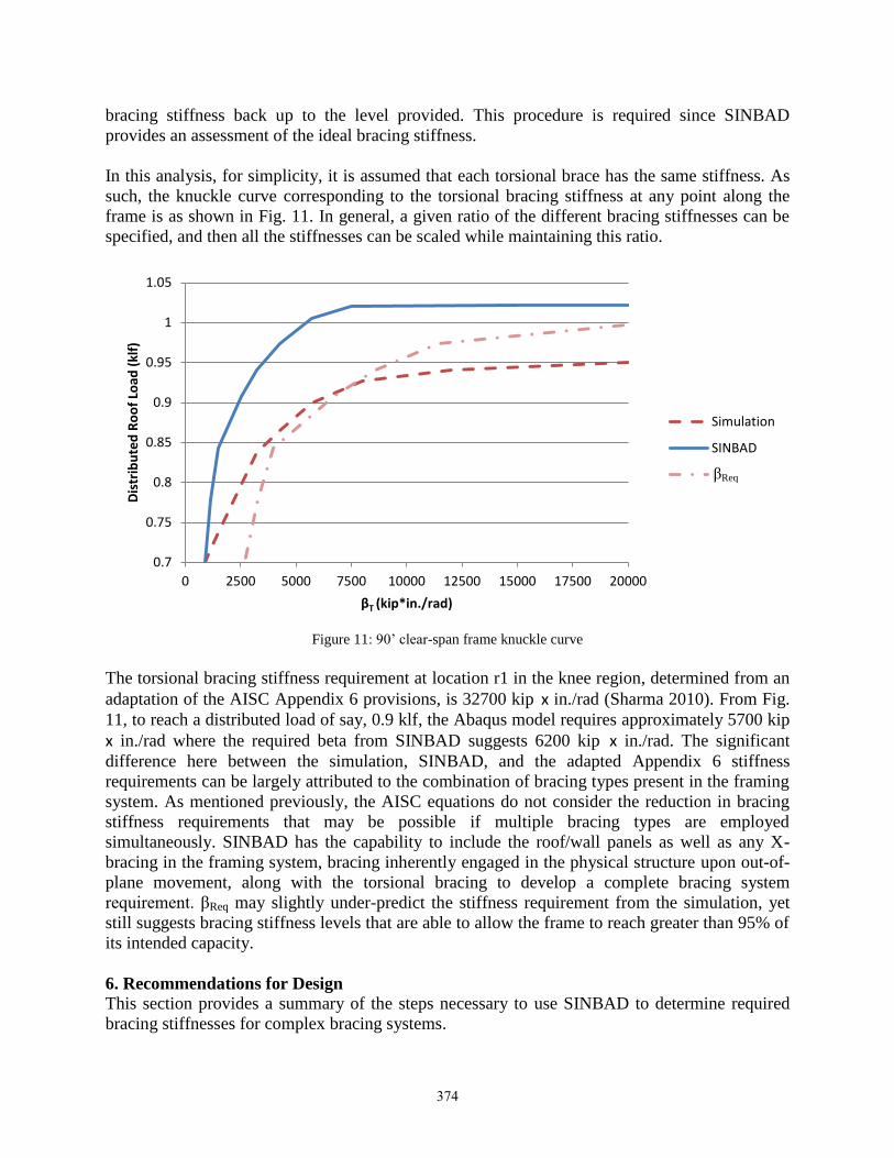
Figure 11: 90’ clear-span frame knuckle curve

The torsional bracing stiffness requirement at location r1 in the knee region, determined from an

adaptation of the AISC Appendix 6 provisions, is 32700 kip x in./rad (Sharma 2010). From Fig.

11, to reach a distributed load of say, 0.9 klf, the Abaqus model requires approximately 5700 kip x in./rad where the required beta from SINBAD suggests 6200 kip x in./rad. The significant

difference here between the simulation, SINBAD, and the adapted Appendix 6 stiffness

requirements can be largely attributed to the combination of bracing types present in the framing

system. As mentioned previously, the AISC equations do not consider the reduction in bracing

stiffness requirements that may be possible if multiple bracing types are employed

simultaneously. SINBAD has the capability to include the roof/wall panels as well as any X-

bracing in the framing system, bracing inherently engaged in the physical structure upon out-of-

plane movement, along with the torsional bracing to develop a complete bracing system

requirement. βReq may slightly under-predict the stiffness requirement from the simulation, yet

still suggests bracing stiffness levels that are able to allow the frame to reach greater than 95% of

its intended capacity.

6. Recommendations for Design

This section provides a summary of the steps necessary to use SINBAD to determine required

bracing stiffnesses for complex bracing systems.

0.7

0.75

0.8

0.85

0.9

0.95

1

1.05

0 2500 5000 7500 10000 12500 15000 17500 20000

Dis

trib

ute

d R

oo

f Lo

ad (

klf)

βT (kip*in./rad)

Simulation

SINBAD

Beta_MaxβReq

374

6.1 Design for all Bracing Types

Set the elastic modulus for design, E* = 0.9E; required for designs according to AISC’s

Appendix 1 (2010b). AISC Appendix 1 is invoked for the in-plane analysis to allow the

use of SINBAD to determine the bracing requirements from an inelastic analysis

independent of individual Specification section checks.

Determine the knuckle curve for the inelastic structure.

o Set the yield strength for design, Fy* = 0.9Fy; required for designs according to

Appendix 1.

o Set all bracing as rigid and iterate the load level until an eigenvalue equal to one

is reached; this gives the rigidly braced strength. Note: if an eigenvalue ≥ 1 cannot

be reached, then consider either adding bracing, changing the size and spacing of

bracing, or increase the section properties of the member that is being braced and

rerun the analysis.

o Pick different values of load level (ensuring they are less than the rigid load level)

and iterate the bracing stiffness until an eigenvalue equal to one is reached.

o Continue this process until sufficient data points are captured to create the

inelastic buckling knuckle curve.

Determine the knuckle curve for the elastic structure.

o Start with the minimum load level obtained from the inelastic analysis and iterate

the bracing stiffness at each load level until an eigenvalue of one is reached.

o Continue this process until sufficient data points are captured to create the elastic

buckling knuckle curve.

Determine βReq.

o Each point on the βReq curve is determined by taking the larger of 3/0.75 times the

elastic stiffness curve or 2/0.75 times the inelastic stiffness curve at each load

level.

o Continue this process until βReq has been created and added to the knuckle curve

plots.

To determine the required stiffness for a given load level: Enter the knuckle curve at the

appropriate load level and move horizontally until intersection with βReq. The value on

the abscissa will be the required stiffness for the relative or torsional brace.

6.2 Consideration of Bracing Strength Requirements

Sharma (2010) conducted extensive studies of the bracing strength and stiffness requirements

using full nonlinear finite element test simulations of complete metal building frames. He

determined that the strength requirements were rarely more than 4% of the corresponding

member internal moment for torsional bracing (as long as the bracing stiffness was reasonably

close to the “knuckle” of the knuckle curve or larger). In fact he found that usually around 2% of

the internal moment was enough to get the member to within 95% of the member’s capacity.

Lastly, he noted that the comparable relative bracing limit was around 1%.

In this research, the key concept is to determine the ideal stiffness directly and use a multiple of

that stiffness as the torsional or relative stiffness requirement. However, if the bracing stiffness is

too low, then substantial amplification of system geometric imperfections can occur. This can

lead to excessive brace point movement and correspondingly excessive brace forces. Since brace

375

point movement is directly proportional to the brace force (i.e., the brace strength requirement),

it is imperative to limit the out-of-plane movement of the brace points. Yura (2001) largely

championed the procedure necessary to scale the ideal bracing stiffness accordingly in order to

limit these brace forces. The AISC Specification (2010b) embodies this by using a factor of 2/

in the bracing stiffness equations. In this paper, all the suggested recommendations require a

minimum multiple of the ideal stiffness of 2/ based on the inelastic structure and 3/ based on

the elastic structure. The computational tool, SINBAD, provides an efficient and rigorous

calculation of the ideal bracing stiffness values.

A review of the bracing strength requirements associated with the suggested Req values scaled

from the SINBAD ideal bracing stiffness values, indicates that for cases including both full

bracing as well as partial bracing (up to certain limits), the percentage of equivalent flange force

is often under 2% for torsional bracing and is closer to 1% for relative bracing. This evidence

corroborates the findings by Sharma (2010).

7. Conclusions

SINBAD incorporates a number of attributes of metal building frames that lie outside the scope

of AISC’s Appendix 6, namely:

Consideration of web-tapered members,

Unequal brace stiffness,

Unequal brace stiffness,

Warping and lateral bending restraint from joints and continuity across brace points,

Combination of bracing types, and

Reduced demands in non-critical regions.

This paper builds on prior work by Yura (1993, 1995, 1996, 2001), Yura and Helwig (2009),

Tran (2009), Kim (2010), and Sharma (2010) and aims to present a method that is based on

sound theory yet is practical for everyday design use. The use of an inelastic eigenvalue buckling

tool (SINBAD) calibrated to extensive simulation studies provides the engineer with a more

accurate means with which to incorporate the above attributes into a safe structural design for the

complex bracing configurations that can occur in general structural steel members as well as

entire structural systems.

Acknowledgments The authors would like to thank the Metal Building Manufacturers Association (MBMA) for

sponsoring this research. Special thanks are extended to the MBMA Research Steering Committee,

which has been instrumental in helping the authors to make this research project a success. The views

expressed in the paper are solely those of the authors and do not necessarily represent the positions of

the aforementioned organizations or individuals.

References AISC (2010a). “Code of Standard Practice for Steel Buildings and Bridges”, American Institute of Steel Construction,

Inc. Chicago, IL. AISC 303-10. AISC (2010b). “Specification for Structural Steel Buildings”, American Institute of Steel Construction, Inc. Chicago,

IL. ANSI/AISC 360-10. ASCE-WRC (1971). “Plastic Design in Steel – A Guide and Commentary”, Manual 41, Welding Research Council and

the American Society of Civil Engineers.

376

Avent, R. R. and Wells, S. (1979), “Factors Affecting the Strength of Thin-wall Welded Columns”, Report Submitted to Metal Building Manufacturers Association, Cleveland, OH, December.

Bathe, K. and Dvorkin, E. (1985), “A Four-node Plate Bending Element Based on Mindlin/Reissner Plate Theory and a Mixed Interpolation,” International Journal for Numerical Methods in Engineering, 21, Pp. 367-383.

Bishop, C.D. (2013). “Flange Bracing Requirements for Metal Building Systems”, Doctoral Dissertation, Georgia Institute of Technology, Atlanta, GA, awaiting publication.

Cook, R., Malkus, D., Plesha, M., and Witt, R. (2002), Concepts and Applications of Finite Element Analysis, John

Wiley and Sons, New York. ECCS (1983). “Ultimate Limit State Calculations of Sway Frames with Rigid Joints,” Technical Working Group 8.2,

Systems, Publication No. 33, European Commission for Constructional Steelwork, November, P. 20. Kaehler, R.C., White, D.W., and Kim, Y.D. (2011). “Frame Design Using Web-Tapered Members”, AISC Steel Design

Guide 25, American Institute of Steel Construction, Chicago, IL. Kim, Y. D. (2010). “Behavior and Design of Metal Building Frames Using General Prismatic and Web-Tapered Steel

I-Section Members”, Doctoral Dissertation, Georgia Institute of Technology, Atlanta, GA. MBMA (2006). Metal Building Systems Manual, Metal Building Manufacturers Association, Cleveland, OH. MathWorks (2011). MATLAB, Software and Help Documentation, Version R2011b(7.13.0.564). McGuire, W., Gallagher, R., and Ziemian, R. (2000), Matrix Structural Analysis, Second Edition, New York: John

Wiley & Sons, Inc. Nethercot, D. A. (1974), “Buckling of Welded Beams and Girders”, Proc. International Association for Bridge and

Structural Engineering, Vol. 57, 291-306. Sharma, A. (2010). “Flange Stability Bracing Behavior in Metal Building Frame Systems”, In Partial Fulfillment of the

Requirements for the Degree, Master of Science in the School of Civil and Environmental Engineering, Georgia Institute of Technology, Atlanta, GA.

Simulia (2011). Abaqus, Software and Users’ Manuals, Version 6.11. Timoshenko, S. and Gere, J. (1961), Theory of Elastic Stability, New York: McGraw-Hill. Tran, D. Q. (2009). “Towards Improved Flange Bracing Requirements for Metal Building Frame Systems”, In Partial

Fulfillment of the Requirements for the Degree, Master of Science in the School of Civil and Environmental Engineering, Georgia Institute of Technology, Atlanta, GA.

White, D.W. (1985). “Material and Geometric Nonlinear Analysis of Local Planar Behavior in Steel Frames Using Interactive Computer Graphics”, In Partial Fulfillment of the Requirements for the Degree, Master of Science, Cornell University, Ithaca, NY, August.

White, D.W. (1988). “Analysis of Monotonic and Cyclic Stability of Steel Frame Subassemblages,” In Partial Fulfillment of the Requirements for the Degree, Doctor of Philosophy, Cornell University, Ithaca, NY, January.

White, D.W., and Kim, Y.D. (2006). “A Prototype Application of the AISC (2005) Stability Analysis and Design Provisions to Metal Building Structural Systems”, Report Prepared for Metal Building Manufacturers Association, January.

Yura, J.A. (2001), “Fundamentals of Beam Bracing,” Engineering Journal, AISC, 38(1), 11-26. Yura, J.A. (1996), ‘‘Winter’s bracing approach revisited,’’ Engineering Structures 8(10), 821-825. Yura, J.A. (1995), “Bracing for Stability – State-of-the-Art,” Is Your Structure Suitably Braced?, 1995 Conference,

Structural Stability Research Council. Yura, J.A. (1993), “Fundamentals of Beam Bracing,” Is Your Structure Suitably Braced?, 1993 Conference,

Milwaukee, Wisconsin, Structural Stability Research Council, Bethlehem, PA, 1-40. Yura, J. A. and Helwig, T. A. (2009). “Bracing for Stability,” Short course sponsored by the Structural Stability

Research Council, North American Steel Construction Conference, Phoenix, AZ, April.

377