practical computing for engineers-v1
TRANSCRIPT

8/6/2019 Practical Computing for Engineers-V1
http://slidepdf.com/reader/full/practical-computing-for-engineers-v1 1/119
1
PRACTICAL PROGRAMMING FOR ENGINEERS
Sergio E. PerezCopyright, Sergio E. Perez, 2005. No part of this document may be reproduced in anyway without the author’s consent.

8/6/2019 Practical Computing for Engineers-V1
http://slidepdf.com/reader/full/practical-computing-for-engineers-v1 2/119
2
Introduction:
Every computer book written for engineers describes how important computing is toengineering, and rightly so. However, this important conclusion is seriously underminedwhen authors use examples that seem to have a tenuous connection to engineering reality.
Open a computing book for engineers and you will likely see example problems such asdetermining leap years, or perhaps determining the distance a randomly walking drunk will cover – interesting perhaps, but not really illustrative of the types of problemsengineers are likely to encounter.
This book introduces the reader to the practical aspects of computing using realengineering principles and problems from thermodynamics, heat transfer, fluidmechanics statics/dynamics, and strength of materials.
This book is written assuming no knowledge of engineering or computing on the part of
the reader, and should be used as early as possible in an engineering curriculum. Readersshould be familiar with very basic calculus: differentiation and basic integration. If theauthors achieved their goal, using this book will greatly simplify and enrich the study of engineering in the sophomore, junior and senior years.
The book first quickly covers some of the basic features of Excel. While not originallyintended as an engineering tool, Excel is very widely used in engineering as well as business, and is quite powerful.
Some engineering texts come with software known as EES (Engineering EquationSolver). This software is extremely useful for solving the types of problems you will runinto in engineering, and the authors believe should be part of any engineer’s “tool box”.Chapters II and III cover the use of EES using some real-world engineering problems.
Matlab is covered in Chapter IV, and is probably the most powerful engineering softwareavailable (Please bear in mind that engineering software is different from programminglanguages such as C++, FORTRAN and Java) – certainly it is becoming the most popular. Why use Matlab if EES is available? You will see that Matlab can do muchmore than EES (but you will also see that for some applications EES is better!).
And finally, last chapter covers some of the basics of Java, C++ and FORTRAN – programming languages that students may run into in their careers.
As a closing remark, the authors would like to point out that this textbook covers only the basics of Excel, EES, and Matlab that you may need to solve engineering problems. Youwill not learn how to highlight cells in different colors in Excel, nor learn about some of the more abstruse methods of matrix inversion using Matlab. Much of this information isavailable from the manuals available with the software. However, we feel that if youconscientiously work your way through this book, you will be able to solve many basic

8/6/2019 Practical Computing for Engineers-V1
http://slidepdf.com/reader/full/practical-computing-for-engineers-v1 3/119
3
engineering problems with considerably less effort than without it, and you will have avery solid programming foundation on which to build.
To use this book you should have the following on your computers: Excel, EES (a trialversion may be downloaded from www.fchart.com), and Matlab.

8/6/2019 Practical Computing for Engineers-V1
http://slidepdf.com/reader/full/practical-computing-for-engineers-v1 4/119
4
Chapter 1.
How computers work.
It seems magical if you think about it, but computers can perform hundreds of thousands
of operations in the time it takes you to blink your eyes - millions of operations per second. They can store huge amounts of information and access that information almostinstantly. How does a computer do it?
Central to the operation of computers is the binary numbering system. We use a base tennumbering system in everyday life, which has repeating cycles of ten – a number is“carried over” every 10th number. Ten distinct numbers are used (0-9). In the binarysystem there are repeating cycles of two numbers (0 and 1), and a number is carried over every two numbers. Two distinct numbers are used (0-1). The table below shows thismore clearly.
Base Ten Binary (Base Two)0 01 12 10 Number carried over 3 114 100 Number carried over 5 1016 110 Number carried over 7 1118 1000 Number carried over 9 1001
10 1010 Number carried over
Number Carried over
The binary digits are referred to as bits (short for binary digits). Eight bits refers to a binary number such as 10010111, which has eight binary digits. A collection of eight bitsis referred to as a byte.
The first personal computers were 16-bit machines; they could work with binary numbersup to sixteen bits in length. With 16 bits, the largest decimal number that can beexpressed is 65,536. If these computers needed to work with larger numbers, they first
needed to break the numbers up into smaller components, perform operations on each of the components, and recombine them for a final answer. This is a relatively slow process.
Today’s personal computers are 32-bit machines. By using 32 digits, they can work directly with numbers as large as 4,294,967,296. The ability to work with 32 digits at atime makes these computers much faster than their predecessors.

8/6/2019 Practical Computing for Engineers-V1
http://slidepdf.com/reader/full/practical-computing-for-engineers-v1 5/119
5
At this point, the binary system may seem like an unnecessary complication. However,the binary system becomes very convenient for expressing numbers using “On” and“Off” pulses, which is very convenient using electronics. The “On” condition refers tothe number 1, while “Off” refers to the number zero. To the computer, a voltage less than2.5 is off, while a voltage greater than 2.5 is on.
For example, say you had 8 current sources, each representing a bit (or digit). By havingthe sources read off, off, off, off, off, on, on, on you would express the binary number 00000111, or 7 in decimal.
A computer can shut a switch on and off extremely fast using transistors –much, muchfaster than you could ever hope to do by mechanical means (in fact, before transistors,computers used mechanical switches to send binary signals). It then becomes possible tovery quickly turn current on-and-off, and thus express numbers using electrical signals.
Transistors are made using semi-conducting materials such as silicon, which is extremely
common in nature. Semi-conductors are neither conductors nor insulators – they conductelectricity better than insulators but not as well as conductors. The semi-conductors arecrystals (atoms bonded in repeating patterns) of silicon that are “doped” or mixed withsmall amounts of impurities. By properly selecting the type of impurity it’s possible tohave an “N” type of semi-conductor (with extra electrons) or a “P” type semi-conductor (with missing electrons).
Transistors are made by making a sandwich of N-P-N or P-N-P semi-conductors, asshown below. The result is a very useful combination that allows extremely fast on-and-off switching of current.
Base
Collector
Emitter
P N P
8/6/2019 Practical Computing for Engineers-V1
http://slidepdf.com/reader/full/practical-computing-for-engineers-v1 6/119
6
Note that three wires are connected into the transistor: the emitter, the base, and thecollector. The remarkable thing about this arrangement is that current will flow from theemitter to the collector only if a small current enters through the base. In other words, wehave an inexpensive way to turn current on and off by letting current flow into the base.Unlike mechanical devices which possess considerable inertia, the switching using
transistors is as fast as the moving electrons.
Before transistors, the same switching was done using tubes about half the size of adrinking glass. Tubes created considerable heat, consumed large amounts of power, andhad a tendency to burn out frequently. They were used in the original computers for calculations for the Manhattan project during World War II, and required large rooms tohouse them. In contrast, transistors can now be miniaturized using integrated circuits sothat millions of them are placed on a personal computer’s postage-stamp-sized processingchip (the brains of the computer). Before tubes, computers were made using mechanicalswitches to cycle on-and-off signals – glacial speeds compared to transistors!
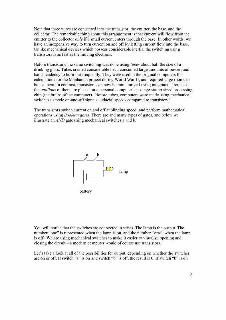
The transistors switch current on and off at blinding speed, and perform mathematicaloperations using Boolean gates. There are and many types of gates, and below weillustrate an AND gate using mechanical switches a and b.
You will notice that the switches are connected in series. The lamp is the output. Thenumber “one” is represented when the lamp is on, and the number “zero” when the lampis off. We are using mechanical switches to make it easier to visualize opening andclosing the circuit – a modern computer would of course use transistors.
Let’s take a look at all of the possibilities for output, depending on whether the switchesare on or off. If switch “a” is on and switch “b” is off, the result is 0. If switch “b” is on
a b
lamp
battery

8/6/2019 Practical Computing for Engineers-V1
http://slidepdf.com/reader/full/practical-computing-for-engineers-v1 7/119

8/6/2019 Practical Computing for Engineers-V1
http://slidepdf.com/reader/full/practical-computing-for-engineers-v1 8/119
8
decimal. We can do any combination of one bit addition using the XOR/ANDcombination.
There are other gates such as OR, AND, NAND, and XNOR gates which can be used inconjunction with the AND and XOR gates to add larger numbers and to perform
multiplication, division and subtraction, as well as other more complicated operations.We won’t go into these, but the bottom line is that the truth table of these gates or combinations of them is the same as the results of adding numbers.
To summarize the last few bits of information:
a) We can perform binary mathematical operations using combinations of Boolean gates.The truth tables of gate combinations are the same as the results of the requiredoperations.
b) Performing these calculations requires turning switches on and off. This is
accomplished very quickly using transistors.
HARD DISK, RAM and the CPU
You can see that ones and zeroes (on and off) are used by the computer to performmathematical operations. In fact, all operations done by your computer are done bymanipulating on and off pulses through gates. However, in addition to having thecapability to perform operations, your computer has to remember what it has done, bothin the short-term and the long-term.
If you have ever tried to add two digit numbers in your head, you probably realize thatthe biggest obstacle to performing the operation is remembering results of previous steps.For example, if you are adding 93+25, it’s easy enough to add the 5 and the 3, but youhave to remember the result of the first step when you move on to the next digit, as wellas any digits to carry over. In addition, your computer can be asked to store results in thelong-term – you really do not want to have to lose that long document when you shut off your computer!
Your computer stores information permanently in the hard disk magnetically, in much thesame way that a tape recorder records sound.
The hard disk consists of one or more platters, covered with a material that can be rapidlymagnetized as either “N” or “S” (on or off!). Recording heads read or write to the disk,although they are not in physical contact with the platter. The platter spins very rapidly, just a few millionths of an inch from the heads.
When your computer is turned off, the magnetic information remains on the disk, and can be later retrieved. The capacity of computers’ hard disks has been rapidly growing sincethe advent of the personal computer. Today’s machines have greater than 2 gigabyte hard

8/6/2019 Practical Computing for Engineers-V1
http://slidepdf.com/reader/full/practical-computing-for-engineers-v1 9/119
9
drives. This means they can store over 2,000 million bytes of eight bits each, or 16,000million “on” or “off” settings.
The problem with storing information on the hard drive is that it takes a “long” time toextract information from it, as compared to the time it takes to make calculations. A
modern personal computer’s processor can perform over one billion operations per second, but the hard drive can only be accessed at a much slower rate!
This is where RAM, or random access memory steps in. Random access memory iswhere information is stored in the short-term. Information stored in RAM is lost when thecomputer is turned off or after a program stops. Unlike the hard disk, RAM storesinformation (ones and zeroes!) electronically inside millions of gates. There is no need towait for the platter to spin to the right location over the heads; the information can beaccessed much more rapidly – about 200,000 times faster than the disk.
When you run any program, such as Microsoft’s Excel or Word, the program is moved
from the hard disk into RAM. This explains why older computers are often incapable of running newer software –there is just not enough capacity to store the program in RAM.
The central processing unit (or CPU) is the heart of your computer, where thecalculations are carried out. When you say you have a 2 gigahertz processor, you arereferring to the millions of transistors/gates inside your CPU that can perform 2,000million operations or cycles (such as adding, subtracting) per second.
The CPU is so fast that it makes RAM even seem slow. To prevent a bottle-neck of information at RAM, there is storage on the CPU chip referred to as the internal cache,which is much faster than RAM. This allows information to flow to and from the CPU ata much faster rate.
8/6/2019 Practical Computing for Engineers-V1
http://slidepdf.com/reader/full/practical-computing-for-engineers-v1 10/119
10
Chapter 2.
EXCEL
Excel is a spreadsheet marketed by Microsoft Corporation. For all the bad press that
Microsoft has gotten as far as its business practices, Microsoft has made it a policy to hirethe best programmers and engineers in the world, and its products reflect the quality of their employees.
Excel is an extremely powerful and easy-to-use spreadsheet that has gained world-wideacceptance in all industries, including engineering. Excel is best suited for engineerswhen the level of calculations is not very sophisticated – as much of engineering work can be. This is not to say that Excel cannot handle complicated calculations – far from it.Excel can be programmed, and “Add-on” tools allow Fourier series analysis, Besselfunctions, complex numbers, solving simultaneous equations and automatic dataacquisition, among others. However, the other tools we will cover are really much better
suited for the more difficult engineering applications.
The power of Excel for engineering applications is best shown by example.
2-D plots and Curve-Fitting
Example 1. Drag force on a submarine.
Naval architects (ship and boat designers) are very concerned with how much force holds back the motion of a vessel moving through the water. Imagine that you were standing onthe seashore and had to pull a boat to shore using a long rope. You can easily envision
that it would take some force to do this. If you really think about it you would concludethat the faster you wanted the boat to move, the harder you would have to pull.
The force that resists the motion of an object through a fluid (for engineers a fluid is a gasor a liquid) is called drag force. The vessel’s engines must provide enough thrust toovercome the drag force, just as your arms had to provide enough pull to move the boat.
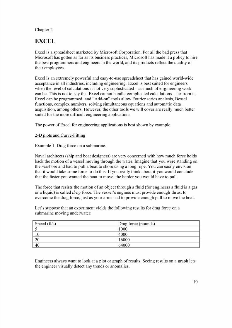
Let’s suppose that an experiment yields the following results for drag force on asubmarine moving underwater:
Speed (ft/s) Drag force (pounds)
5 100010 4000
20 16000
40 64000
Engineers always want to look at a plot or graph of results. Seeing results on a graph letsthe engineer visually detect any trends or anomalies.
8/6/2019 Practical Computing for Engineers-V1
http://slidepdf.com/reader/full/practical-computing-for-engineers-v1 11/119
11
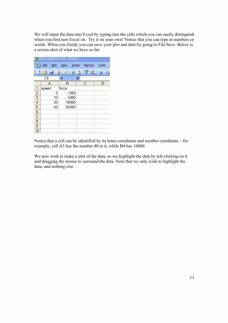
We will input the data into Excel by typing into the cells which you can easily distinguishwhen you first turn Excel on. Try it on your own! Notice that you can type in numbers or words. When you finish, you can save your plot and data by going to File/Save. Below isa screen-shot of what we have so far:
Notice that a cell can be identified by its letter coordinate and number coordinate – for example, cell A5 has the number 40 in it, while B4 has 16000.
We now wish to make a plot of the data, so we highlight the data by left-clicking on itand dragging the mouse to surround the data. Note that we only wish to highlight thedata, and nothing else. :

8/6/2019 Practical Computing for Engineers-V1
http://slidepdf.com/reader/full/practical-computing-for-engineers-v1 12/119
12
We now tell Excel to plot the data by clicking on the Plot icon located in the toolbar attop:
You then select x-y scatter plot (there are many others), which will show the data pointsand connect them with smooth lines:

8/6/2019 Practical Computing for Engineers-V1
http://slidepdf.com/reader/full/practical-computing-for-engineers-v1 13/119
13
Click “Next”, which will give you the screenshot below. You can see your data are presented in graphical format (by the way, data is plural, although the singular appears to be gaining acceptance).
You can now type in a title for the plot, as well as a title on the x and y axes. It isextremely important that you specify the units that are being used on each axis! A fewmonths down the line you might need to revisit your plot and know exactly what wasgoing on! In addition, if your plot is intended to be part of a report, YOU MUSTSPECIFY THE UNITS on each axis so that anyone reading your report will know exactlywhat you are talking about.

8/6/2019 Practical Computing for Engineers-V1
http://slidepdf.com/reader/full/practical-computing-for-engineers-v1 14/119
14
For the title you might write “Drag Force on a Submarine”, “Speed (ft/s)” might be good
for the x-axis, and “Drag (lbf)” is adequate for the y-axis.
By clicking on the tabs seen at the top of the screenshot above you can further adjust your plot.------------------------------------------------------------------------------------------------------------Homework #1Become familiar with the axes, gridlines, legend and data labels commands in the tabsabove. Know what they do and how to use them. You may wish to use the ‘Help’command in the toolbar.
Click “Next”, and select to display the plot as an object in Sheet 1 (the name Excel
automatically gives to the spreadsheet you are working on), then “Finish”. The screenshot below shows the results so far.

8/6/2019 Practical Computing for Engineers-V1
http://slidepdf.com/reader/full/practical-computing-for-engineers-v1 15/119
15
Nice plot! You can print it by clicking on the plot outline (the border!) and going to“Print” in the toolbar. You can also copy the plot into a document by keying “Ctrl + C” to paste the document into the clipboard, and then by keying “Ctrl+V” into your document.
Your plot probably has a “Series 1” drawing on the right. This is for distinguishing between multiple plots on one graph, and was eliminated from this plot by right-clickingon “Series 1” and deleting it.
You may save the spreadsheet and plot by clicking on “Save” in the toolbar at top.
Now we wish to do something extremely useful for engineers, which is to come up withan equation for the plot. In other words, we want a formula that gives us the drag force,given the speed. This is known as curve-fitting .
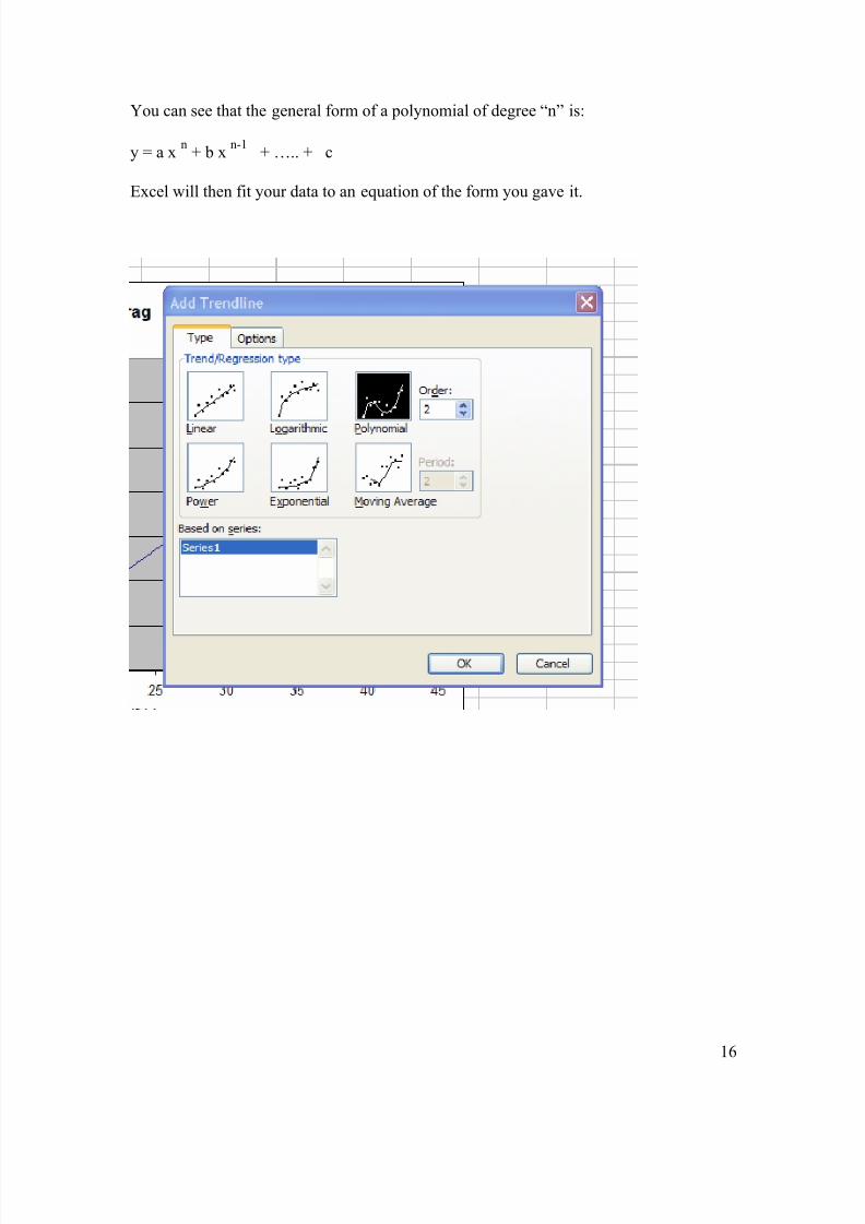
Right-click on the graph line (the plot itself which Excel drew). Select “Add Trendline”.
You will see several selections: linear, power, exponential, logarithmic, moving averageand polynomial.
Select “Polynomial”, 2nd order. Some examples of polynomials are:
y = 5.67 x3
+ 3.45 x2
+ 1.1 x + 35 (a third degree polynomial)
y = .45 x2
- 9.1 x + 3.9 (a second degree polynomial)
8/6/2019 Practical Computing for Engineers-V1
http://slidepdf.com/reader/full/practical-computing-for-engineers-v1 16/119
16
You can see that the general form of a polynomial of degree “n” is:
y = a xn
+ b xn-1
+ ….. + c
Excel will then fit your data to an equation of the form you gave it.

8/6/2019 Practical Computing for Engineers-V1
http://slidepdf.com/reader/full/practical-computing-for-engineers-v1 17/119
17
Note the equation is printed on the plot. The equation is:
y = 40 x2
– 1E-11 x + 2E-10
The “E” refers to exponentiation: 1E-11 means 1 x 10-11 . Notice that this is an extremely
small number compared to the data and the other numbers in the equation, as is the last
number. The equation may be written as y = 40 x2.
In other words, you now have an equation for y, given x. If you substitute into thisequation a value of x of 20 the result will be 16,000.
If you look at the plot carefully you will notice there appear to be two lines: a blue lineand a darker black line. The lighter blue line is the original estimated best line throughyour data automatically drawn in by Excel. The black line is your fit to the data – also
automatically made by Excel by plugging many, many values of x into the equation youasked it to generate.
Two words of caution here:
a) We decided that the last two terms in the equation were insignificant, and rightly so.However, you should be careful when dropping terms, in that they may be significant if

8/6/2019 Practical Computing for Engineers-V1
http://slidepdf.com/reader/full/practical-computing-for-engineers-v1 18/119
18
they are multiplied by large numbers. For example, an expression like 1E-5 x may seemsmall, but if x is very large, then the term may be significant.
b) Be careful when using your equation beyond the range of the fitted data. In other words, the values of x that you gave Excel ranged from 5 to 40. If you then try to use the
equation for values of x greater than 40 or less than 5, you may get unrealistic results,since the original experimental data never went outside of this range.
Always look at your fit. Does the dark line appear faithful to the general trend of the data – in other words, if you had to sketch in the values in-between your data points, wouldyour sketch appear similar to the plot line drawn by Excel? If the plot line appears good,then you can conclude that you made a good selection when you selected a polynomial fitof 2nd order. If however, you are not satisfied with the way the plot looks, you can try ahigher order, or even a different type of fit.
In general, you should always use the smallest polynomial that represents the data well.
However, you cannot expect too low an order to fit a complicated curve; a 1
st
degree polynomial does not curve (it’s just a straight line of form y = mx+b) , a 2nd degree polynomial curves once, a 3rd degree can curve twice… you get the picture. Do keep inmind that to fit a second degree polynomial you need three data pair, a third degreerequires four, etc.
As mentioned above, the higher the order, the better you can get the fit to go through thedata points. However, keep in mind that you may not want your fit to follow every single”wiggle” in the data – particularly if the data are the result of an experiment where theymay be some scatter in the data. Looking at the fit and visually determining if the fit isrealistic is probably the best way to ensure you are not producing garbage!
Occasionally, if you use too high an order for the polynomial, your fit will go throughevery single data point, but loop unrealistically in-between the data points. One of the problems deals with this very important issue.
------------------------------------------------------------------------------------------------------------Homework/class activity:1) Fit the data from the previous example to a 1st degree polynomial. What does the fitlook like? Is it a good representation of the data?2) Try a 3rd degree and fourth degree polynomials. Do they seem like good fits? What doyou conclude about the coefficients in the equation?3)What is the highest degree you could use for these data?4) Try a power and a log fit to the data. What are the resulting equations, and do theyappear to fit the data well?5) Of all the fits you tried, which appears to be the best?

8/6/2019 Practical Computing for Engineers-V1
http://slidepdf.com/reader/full/practical-computing-for-engineers-v1 19/119
19
Mathematical Operations in Excel, Hierarchy of Operations, Unit Consistency,
Integration by Curve-Fitting
A gas expands inside a piston/cylinder arrangement, so that the piston moves up as thegas expands. The following pressure and volume readings are taken:
P (psia)Vol(ft^3)
10 2
8 2.5
6 2.7
4 2.8
2 2.85
We wish to find the work done by the gas. From thermodynamics we know that the work done by a gas is given by the area under the P-V plot (that is, the work is the integral of PdV), so all we have to do is make a plot of the data and find the area under the curve.This becomes particularly easy if we make a polynomial fit to the data, and just do the
integral.We plot the data and make a 3rd degree polynomial fit:
Chart Title
y = -0.0026x3 + 0.029x2 - 0.1315x + 3.02
R2 = 0.9993
0
0.5
1
1.5
2
2.5
3
0 2 4 6 8 10 12
Notice that the curve fit does not exactly go through all of the data points. Since therewas probably some measurement errors in the experiment, we will not be too concernedwith making sure every data point is exactly reproduced by the fit.
Notice also that Excel is also giving us a R 2
value. R is a number referred to as the
“residuals”, and is an indication of the quality of a fit. R 2
can have values from 0 to 1,
where 1 is the highest possible quality of the fit, hitting all the data points exactly. You
8/6/2019 Practical Computing for Engineers-V1
http://slidepdf.com/reader/full/practical-computing-for-engineers-v1 20/119
20
can make Excel show you the residuals by left-clicking on the fit curve, selecting“Format Trendline/ Options/ Display R squared value on chart”.
The integration is now easily done due to the simple format of polynomials:
85.2
2
2342
102.31315.3/029.4/0026. x x x x PdV W
V
V +−+−== ∫
The integral is evaluated by first substituting 2.85 into the formula, then substituting 2into the formula, and then subtracting the second result from the first.
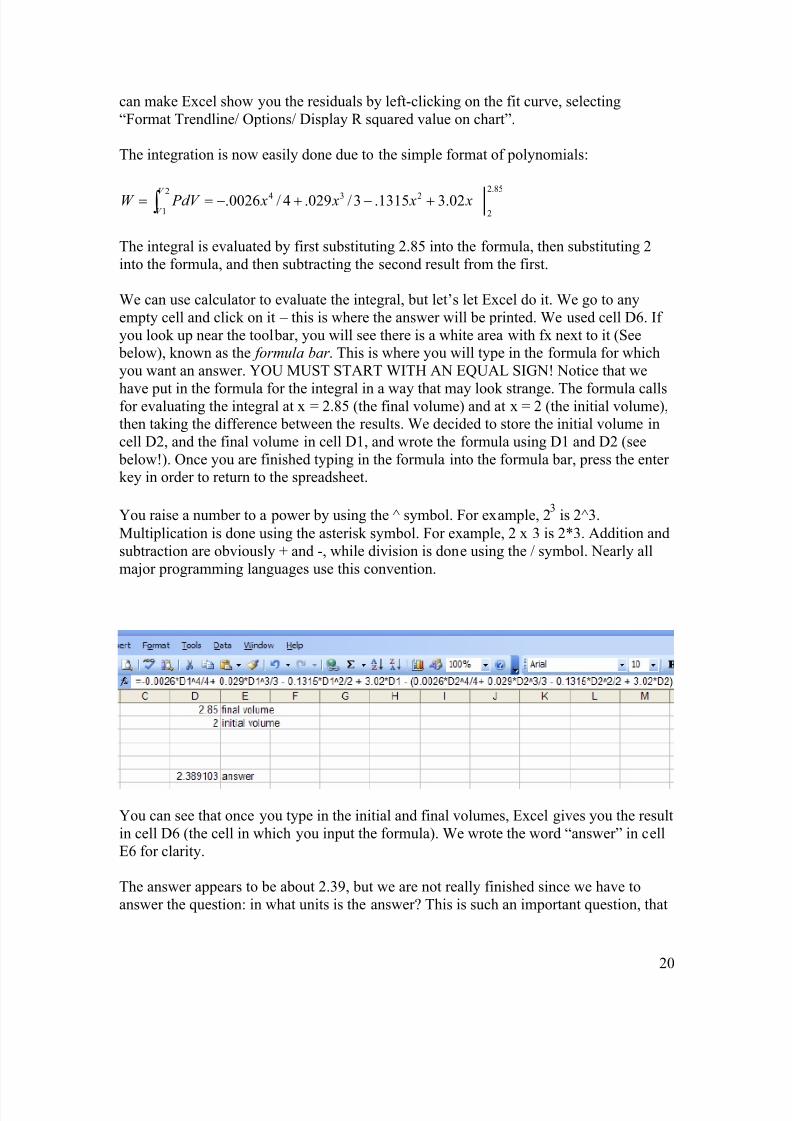
We can use calculator to evaluate the integral, but let’s let Excel do it. We go to anyempty cell and click on it – this is where the answer will be printed. We used cell D6. If you look up near the toolbar, you will see there is a white area with fx next to it (See below), known as the formula bar . This is where you will type in the formula for whichyou want an answer. YOU MUST START WITH AN EQUAL SIGN! Notice that we
have put in the formula for the integral in a way that may look strange. The formula callsfor evaluating the integral at x = 2.85 (the final volume) and at x = 2 (the initial volume),then taking the difference between the results. We decided to store the initial volume incell D2, and the final volume in cell D1, and wrote the formula using D1 and D2 (see below!). Once you are finished typing in the formula into the formula bar, press the enter key in order to return to the spreadsheet.
You raise a number to a power by using the ^ symbol. For example, 23
is 2^3.
Multiplication is done using the asterisk symbol. For example, 2 x 3 is 2*3. Addition andsubtraction are obviously + and -, while division is done using the / symbol. Nearly allmajor programming languages use this convention.
You can see that once you type in the initial and final volumes, Excel gives you the resultin cell D6 (the cell in which you input the formula). We wrote the word “answer” in cellE6 for clarity.
The answer appears to be about 2.39, but we are not really finished since we have toanswer the question: in what units is the answer? This is such an important question, that

8/6/2019 Practical Computing for Engineers-V1
http://slidepdf.com/reader/full/practical-computing-for-engineers-v1 21/119
21
although not really part of an engineering computing course, it should be addressed heresince it is such an important engineering issue.
Since work is the integral of PdV, and P has units of lb/in^2, and volume has units of ft^3, then the solution units must be lb-ft^3/in^2. This is not a good situation since we are
mixing inches and feet – at any rate the resulting units do not look like anything we areused to seeing as far as work units!
We then convert the lb/in^2 to lb/ft^2 by multiplying the answer by 144 ( there are 144square inches per square foot). We can do this in two ways: by making a new cell withthe right answer, or by modifying the formula.Let’s do it by typing in a formula into cell D7. Check it out below – all we are doing istelling Excel to multiply the result in D6 by 144:
The answer is now 344 ft-lb, which is a much more reasonable number as far as units areconcerned.
The second way of getting the proper answer is by altering the formula in D6. This is a pretty obvious idea, but it does open another very important item – hierarchy of
operations. This is a very fancy-sounding name for a simple concept. If you take a look again at our formula in cell D6, reproduced below, you might ask the question: how doesExcel know which operation to do first? For example, take a look at the D1^4/4 term,which means “the value in cell D1 raised to the 4th power, then divided by 4”.

8/6/2019 Practical Computing for Engineers-V1
http://slidepdf.com/reader/full/practical-computing-for-engineers-v1 22/119
22
What if Excel had first divided the number 4 by 4, and then raised D1 to that number?Excel will not do this because there is a hierarchy or order of operations. In Excel and allof the software and languages we will study, operations are performed in the followingorder:
Hierarchy of OperationsFirst: anything in parenthesesSecond: exponentiationThird: multiplication or division (whichever it sees first from left to right)4th: addition and subtraction (whichever it sees first from left to right).
So, you can see that Excel would have known that D1 had to be first raised to the 4th power, then the result of that operation is divided by 4.
If we now wish to multiply the entire result by 144, we simply add parentheses to theentire expression: one at the beginning, and one at the end:
=(-0.0026*D1^4/4+ 0.029*D1^3/3 - 0.1315*D1^2/2 + 3.02*D1 - (0.0026*D2^4/4+0.029*D2^3/3 - 0.1315*D2^2/2 + 3.02*D2))*144
Note the previous expression (before multiplying by 144) had been:
=-0.0026*D1^4/4+ 0.029*D1^3/3 - 0.1315*D1^2/2 + 3.02*D1 - (0.0026*D2^4/4+0.029*D2^3/3 - 0.1315*D2^2/2 + 3.02*D2)
Homework Use a calculator to determine the result of the following operations.
1) 2^3/8+10/52) 3-8*2-(3*2)3) 10-3/(8-6)4) (10-3)/(8-6)5) 10*3/5-6
Example 3: Tank Ullage Readings in a leaking oil tanker. (How a formula isautomatically copied into other cells)
An oil tanker is leaking oil from one of its tanks. The crew members measure the amountof oil in each tank by dipping a tape into the oil from above, and then measuring thedistance from the top of the tank to the oil/air interface. These are known as ullage
readings. We put the ullage readings into an Excel spreadsheet:
TankUllage(ft)
1 2.1
2 2.7
8/6/2019 Practical Computing for Engineers-V1
http://slidepdf.com/reader/full/practical-computing-for-engineers-v1 23/119
23
3 4.6
4 2.6
5 2.7
We wish to know how much oil is remaining in each tank, in barrels. We are told by the barge operator that there are 32.2 barrels per inch in each tank, and that the top of thetanks is 25 feet from the bottom of the barge.
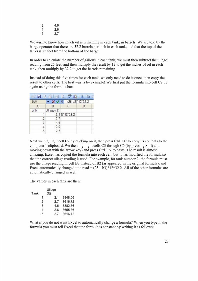
In order to calculate the number of gallons in each tank, we must then subtract the ullagereading from 25 feet, and then multiply the result by 12 to get the inches of oil in eachtank, then multiply by 32.2 to get the barrels remaining.
Instead of doing this five times for each tank, we only need to do it once, then copy theresult to other cells. The best way is by example! We first put the formula into cell C2 byagain using the formula bar:
Next we highlight cell C2 by clicking on it, then press Ctrl + C to copy its contents to thecomputer’s clipboard. We then highlight cells C3 through C6 (by pressing Shift andmoving down with the arrow key) and press Ctrl + V to paste. The result is almostamazing. Excel has copied the formula into each cell, but it has modified the formula sothat the correct ullage reading is used. For example, for tank number 2, the formula mustuse the ullage reading in cell B3 instead of B2 (as appeared in the original formula), andExcel automatically changed it to read = (25 – b3)*12*32.2. All of the other formulas areautomatically changed as well.
The values in each tank are then:
TankUllage(ft)
1 2.1 8848.562 2.7 8616.72
3 4.6 7882.56
4 2.6 8655.36
5 2.7 8616.72
What if you do not want Excel to automatically change a formula? When you type in theformula you must tell Excel that the formula is constant by writing it as follows:

8/6/2019 Practical Computing for Engineers-V1
http://slidepdf.com/reader/full/practical-computing-for-engineers-v1 24/119
24
=(25 - $B$2)*12*32.2
In other words, by inserting the $ sign before and after the cell letter, we tell Excel tomake the formula fixed.
Average/Standard Deviation
Example 4: Averages, Standard deviation
You are trying to find the tension yield point of a composite material you have invented.The yield point is the point at which the material begins to deform very rapidly under aload. For example, if you put a small tension load on a sample material, it might stretch asmall amount. If you continue to load the material it will continue stretching a smallamount, until you reach a high enough load that the material begins stretching much morefor the same amount of increase in the load. The material has reached its yield point, and
if you were to remove the load, it would not return to its original length – the deformationis permanent. Removing the load before the yield point is reached would result in thespecimen returning to its original length.
Below are some results for yield point of your specimen after ten trials. The specimen iscircular, and measures 1.5 cm in diameter. The results are in newtons (by the way, a Newton is equivalent to about ¼ lb).
TrialYield(N)
1 5000
2 5010
3 49004 4980
5 5300
6 4920
7 5003
8 5010
9 4987
10 4870
We wish to know the average value of the yield point, which is extremely easy withExcel. The yield values are in cells B2 through B11. Go to any empty cell and type in theformula bar:
= AVERAGE(B2:B11)
The command tells Excel to take the average of cells B2 through B11:
TrialYield(N)
1 5000

8/6/2019 Practical Computing for Engineers-V1
http://slidepdf.com/reader/full/practical-computing-for-engineers-v1 25/119
25
2 5010
3 4900
4 4980
5 5300
6 4920
7 5003
8 50109 4987
10 4870
average 4998
However, the average is not enough when presenting the results of an experimentconsisting of several trials. We are always interested in how consistent the data are – inother words, do the results change significantly from one trial to the other? If they didyou might conclude that your average must be looked at with great care.
One way to judge the results of a test involving many results is through the standarddeviation. The standard deviation is given by the formula:
You can think of the standard deviation as a measure of the average deviation of eachtrial from the average value of all the trials. Although it gives a value that is slightlydifferent from average deviation, this is a good way to look at the standard deviation.
To get the standard deviation of the data using Excel is simplicity itself. Just type into theformula bar for an empty cell:
=stdev(b2:b11)
Here is the result:
Trial Yield (N)
1 5000
2 5010
3 4900
4 4980
5 5300
6 4920
7 50038 5010
9 4987
10 4870
average 4998sdeviation 117.3968

8/6/2019 Practical Computing for Engineers-V1
http://slidepdf.com/reader/full/practical-computing-for-engineers-v1 26/119
26
This deviation of 117.3968 must be compared in magnitude to the yield values. 117 outof the average of 4998 is roughly 2%. In other words, the data vary by an average of about 2% of the mean, which is probably an acceptable deviation (of course, this dependson your particular requirements).
Incidentally, you could also take an average or a standard deviation going sideways(across a row). For example, say you wanted the standard deviation of the values in cellsA2 to D2, you would simply type in:
stdev(A2:D2)
Solving Equations (Root-Finding) by Iteration
Example 5: Solving an equation by iteration
There are many equations which are “unsolvable” analytically. By analytically we mean
using the usual algebraic techniques. However, equations may be solved numerically,which means by approximate methods. Approximate methods can be as accurate as youwant them to be, as you will soon see.
We don’t have to search very far for an unsolvable equation. You may recall we came upwith the equation for V as a function of P earlier:
V =-0.0026*P^3+ 0.029*P^2 - 0.1315*P + 3.02
What if we were asked to solve for the pressure P, given a volume of 2.65? If you stare atthe equation long enough you will soon see that it’s a tough one! It may be possible tosolve analytically – perhaps you have the time to contact someone in the mathematicsdepartment. However, it is pretty easy to solve this equation using Excel. Solving thisequation is also known as root-finding, or finding out where the equation above crossesthe zero point, if we move the V to the right hand-side:
-0.0026*P^3+ 0.029*P^2 - 0.1315*P + 3.02 - V
We will solve the equation in the original form.
The procedure is simple: you guess values of P until V is equal to 2.65. All you need is arough idea of where the answer is going to be, as there are probably three answers, sincethe equation is a cubic – that is, it has a third power in it. An equation with a second power has two possible solutions, and one with an exponent to the 1st power has only onesolution. You get the pattern.
We go to Excel and type the formula into cell A1, making the P guess in D1. After a fewtries we see the solution appears to be about 6.8:

8/6/2019 Practical Computing for Engineers-V1
http://slidepdf.com/reader/full/practical-computing-for-engineers-v1 27/119
27
This was a bit of work. We can automate the process by telling Excel to try values of Pfrom 6. 7 to 6.9 in increments of, say 0.01. You can do this by typing the formula “ =6.7” in cell A4, then in cell A5 typing in the formula “ = A4 + 0.01 “. You would thencopy this formula into 200 cells below, which you will remember will result in Excelappropriately changing the formula in each row.
Don’t worry about running out of rows. Excel allows 65,356 rows, and 256 columns!--------------------------------------------------------------------------------------------------------Homework: Finish the problem above, automatically coming up with an answer that isaccurate to within 0.01.--------------------------------------------------------------------------------------------------------Problem: Solve the following equation for x if y = 4 using your computer, between 0 and-0.2.:
y = 3x2
+ 14x – 3
Do this automatically so Excel will try values from 0 to -0.2 in steps of -0.001. In other
words, set up the formula in one cell, and copy it into many cells below it, trying valuesof x from 0 to -0.2.--------------------------------------------------------------------------------------------------------
Trigonometric and Other Functions
Excel calculates trigonometric functions with the following commands. Keep in mindthat Excel takes angles in radians. There are 2 pi radians per 360 degrees, so you canconvert from degrees to radians by multiplying by pi/180. Excel will recognize thenumber pi, but you must specify it as pi():
Tan(10* pi()/180) = tan of 10 degreessin(2) = sin of 2 radianscos(2) = cos of 2 radianstan(5) = tangent of 5 radians
OK… you get the picture. For more trigonometric functions, please see the Help menu inExcel.

8/6/2019 Practical Computing for Engineers-V1
http://slidepdf.com/reader/full/practical-computing-for-engineers-v1 28/119

8/6/2019 Practical Computing for Engineers-V1
http://slidepdf.com/reader/full/practical-computing-for-engineers-v1 29/119
29
We use Newton’s 2nd law. We arbitrarily give the 500 N downward force a positive signfor its direction, and the upwards drag force of .07V^2 is given a negative sign:
∑ = ma F
dt mdV V /2^07.500 =−
Note that we have replace the acceleration a by dV/dt. We now have a differentialequation. If you have never seen one before, congratulations on your new-found
discovery! A differential equation is just an equation with a derivative in it.
Next we can approximate the dV/dt term by using finite differences, as follows:
t V V t V dt dV initial final ∆−=∆∆≈ /)(//
In words, dV/dt is approximated by the change in velocity over a time interval (which wewill choose. This will give accurate results as long as the time interval is small.
So, as a simpler example, if the drag force is 100, the mass is 100, the time interval is 0.1s, and the speed at the beginning of the time interval is 1, we can solve for the final speedat the end of the 0.1 s:
dT mdV ma F /==∑
1.0/)1(100100500 −=− final V
We can easily solve for the Vfinal at the end of the 0.1 s as 41.
500 N
0.07 V^2

8/6/2019 Practical Computing for Engineers-V1
http://slidepdf.com/reader/full/practical-computing-for-engineers-v1 30/119
30
In order to finish the problem we only need to keep marching forward in time so that thefinal velocity of one time step becomes the initial velocity for the next time step.
The sample problem we just did was simpler than the actual problem we are doing,
because the drag force is not a constant 100. The drag force is 0.07*V^2… in other words, the drag force depends on the velocity itself, which is what you are trying to findat each time step!
The solution is to use the previous time step’s velocity to calculate the drag force, and if your time steps are small enough you will not have significant errors. How do you knowif your time step is small enough? If you repeat your calculations at a smaller time step,and you see no change in the solution, then you know you do not need to go any smaller time step!
One thing to keep in mind when you are marching forward in time like this: if you make
the time step too large your solution will blow up, in the sense that after a few time stepsyou will have an astronomically large result. In other words, if you make the time steplarge you will get inaccurate answers, but if you make it too large your solution will blowup.
Let’s set up the equations now. We want to have many increments of 0.1 seconds, whichwe could laboriously type into Excel. We are not sure how many yet, since we do notknow how long it will take to reach terminal velocity, but let’s do 1000 time steps and seeif we reach a constant speed.
We re-write Newton’s 2nd Law, inputting the expressions for the weight, drag force, andacceleration:
t V V mV initial final ∆−=− /)()*07.500( 2
We solve for the velocity V at the end of the time step:
initial final V mt V V +∆−= /)*07.500( 2
We will march forward in time, using the previous time step’s velocity to calculate thedrag force 0.07 V^2. The mass m is 100 kg, and the time step is 0.1 s. Again, the previoustime step’s final velocity becomes the next time step’s initial velocity. Let’s do the firstfew time steps here so you can get a better idea of what is going on:
Time V at end of time step0 0

8/6/2019 Practical Computing for Engineers-V1
http://slidepdf.com/reader/full/practical-computing-for-engineers-v1 31/119
31
0.1 05.00100/1.0)0*07.500( 2 =+−= final V
0.2 45.005.0100/1.0)05.0*07.500( 2 =+−= final V
0.3 45.100/1.0)45.*07.500( 2 +−= final V
And so on.
Programming this in Excel is pretty simple, since you only need to write the formula for one cell, then copy it to all the others.
The mass is in cell D2, and the time step is in cell E2. We then put the following formulain cell B4, to the left of cell C4:
=(500-0.07*B3^2)*$E$2/$D$2 + B3
Note that B3 is the velocity in the previous time step.
We then copy the formula into the cells beneath it and we are finished. Excelautomatically adjusts the formula so that the formula always uses the cell above it tocalculate the drag force and the velocity at the beginning of the time step.
A B C D EMass deltat(s)
time m/s 100 0.1
0 0
0.1 0.5 Cell C4
0.2 0.999983
0.3 1.499913
0.4 1.999755
0.5 2.499475
0.6 2.999038
0.7 3.498408
0.8 3.997551
0.9 4.496433
1 4.995018
1.1 5.493271
1.2 5.991159
1.3 6.488646
1.4 6.985699
1.5 7.482283
1.6 7.978364
1.7 8.473908
The spreadsheet above only shows the first few time steps. It took about 700 time steps or about 70 s to reach the terminal velocity of 84.5 m/s. The end of the spreadsheet is shown

8/6/2019 Practical Computing for Engineers-V1
http://slidepdf.com/reader/full/practical-computing-for-engineers-v1 32/119
32
below, with the elapsed time on the left, and the velocity at right. You can see that thevelocity is still increasing, but very slightly.
69.7 84.47292
69.8 84.47342
69.9 84.47392
70 84.47441
70.1 84.47489
70.2 84.47537
70.3 84.47585
70.4 84.47632
70.5 84.47678
70.6 84.47724
70.7 84.47769
Homework/Projects:1) Use a time step of 0.05 s, and compare the velocity after 30 s with that obtained using
0.1 s. Keep in mind that you will have to take twice as many time steps to reach 30 s if the time step is half as big! Have your program print the elapsed time so that it is easy for you to compare the velocities, as in the spreadsheet above. What conclusion do you reachabout the size of the time step?2) Calculate the terminal velocity of a sphere floating from the bottom of the ocean. Thesphere’s weight is 50 lb. It’s volume is 1 cubic foot. The density of seawater is 64 lb per cubic foot, and the buoyant force on the sphere is equal to the weight of the displaced
fluid (64 lb). The drag force on the sphere is 0.3V2. This problem is essentially the same
as the previous one, but you must now include the additional force due to buoyancy. Alsokep in mind that the mass must be divided by the gravitational constant 32.2 in order for F =ma to work properly.
3) A 40 kg rock is launched directly upwards at a speed of 3 m/s. If the drag force on therock is 0.001 V^2, calculate the height reached by the rock. In this problem you mustkeep track of the total distance covered at each time step. When the velocity of the rock iszero (or about zero) you know you have reached the apogee.
SOLVING SIMULTANEOUS EQUATIONS
Don’t use Excel, it’s like going from NY to NJ via California! But if you must, thediscussion below will show you how.
Excel has the capability to solve large sets of simultaneous equations. We will illustratethe technique by solving a heat transfer problem.
We want to solve for the temperatures at the faces of the slab if it is exposed to movingair at either face, as shown by the diagram below. The slab has a uniform temperature oneach face, and the air has temperatures of 30 and 90 F on the left and right faces. An ovenwall at left has a temperature of 1000 R (to covert from F to Rankine, add 459):

8/6/2019 Practical Computing for Engineers-V1
http://slidepdf.com/reader/full/practical-computing-for-engineers-v1 33/119
33
You might ask yourself why T1 is not equal to the air temperature around it. The reasonfor this is that the wall is being cooled by the other face, which is exposed to 30 F air. Inaddition, the hot oven wall is radiating energy to the slab. the same way, T2 is not equalto the temperature of the surrounding air.
There are three modes of heat transfer occurring in this case. Conduction is occurringthrough the solid slab. Conduction heat transfer is what happens when a solid is exposedto a temperature gradient (that is, a temperature difference).
Convection is occurring on the right and left faces of the slab. Convection heat transfer iswhat occurs when you have a temperature gradient and a fluid is involved (recall a fluidis a liquid or a gas). Bottom line: if a fluid is involved, it’s convection.
Radiation heat transfer is occurring between the slab and the hot oven wall. Radiation isenergy emitted due to an object’s temperature, and requires no medium – the sun’sradiant energy reaches us through millions of miles of vacuum in space. Thermalradiation is not to be confused with nuclear radiation.
The conduction heat transfer Q through the slab is given by the equation:
Qcond = 100*(T1 – T2)
Please note the number 100 is a constant that only applies to this particular problem. Theconstant includes the thickness of the slab and the thermal conductivity of the slab.
The convection heat transfer on the left wall is given by the equation:
Qleft = 5* ( 90 – T1)
Wind = 10 ft/s
Tair = 90 F
Wind = 20 ft/s
Tair = 30 F
T = 1000 R T1 T2
8/6/2019 Practical Computing for Engineers-V1
http://slidepdf.com/reader/full/practical-computing-for-engineers-v1 34/119
34
Where T1 is the temperature of the left wall, and 90 is the air temperature to which thewall is exposed. The constant 5 is a constant particular to this problem only, and dependson the speed of the moving air.
The convection heat transfer on the right wall is given by:
Qright = 25* (T2-30)
Notice this equation is very similar to the one before it. The constant is bigger becausethe air is moving faster over this face, thus increasing the rate of heat transfer. The order of the delta T term was changed to ensure all the terms are positive.
The radiation heat transfer between the hot oven wall and the slab is (assuming that all of the heat leaving each object by radiation lands on the other):
Q rad = 1.712E-9 * (Toven^4 – T1^4)
The 1.712E-9 is the Stefan-Bolzmann constant, which governs radiative heat transfer. Note that radiation depends on the wall temperatures to the 4th power – it becomes verysignificant when temperatures get high!
We can now make several statements which will give us our final simultaneousequations:
The total heat flowing into the left wall is the sum of radiation plus convection, so:
Qtotal = 1.712E-9 * (Toven^4 – T1^4) + 5* ( 90 – T1) [1]
The total heat going into the wall also flows through the wall by conduction, so:
Qtotal = 100*(T1 – T2) [2]
The total heat flowing through the slab equals the heat being convected at the right face:
Qtotal = 25 *(T2 – 30) [3]
We then have three equations and three unknowns: Qtotal, T1, and T2.
We re-arrange equations 1, 2, and 3 so that we have a constant on the left-hand-side of the equation:
From equation 1: 1.712E-9 *Toven^4= Qtotal – 5*(90-T1) +1.712E-9*T1^4
or 1176.2 = Qtotal – 5*(90-T1) + 1.712E-9*(T1+459)^4 [1a]

8/6/2019 Practical Computing for Engineers-V1
http://slidepdf.com/reader/full/practical-computing-for-engineers-v1 35/119
35
Note that we have added 459 to T1 because we need the absolute temperature in Rankine.
From equation 2: 100 = Qtotal/(T1-T2) [2a]
From equation 3: 25 = Qtotal/(T2 – 30) [3a]
Now that we have a constant on one side of each of the equations, we can simultaneouslysolve [1a], [2a], and [3a] using Excel.
We first input guesses for the unknowns qtotal, T1, and T2 into spreadsheet cells B7, B8,and B9.
Next we input equations 1a, 2a, and 3a into cells B2, B3, and B4. Cell D2 has the oventemperature of 1000 R.
A B C D
Equations 1 Oven
200.1123243 2 1000
5 3
10 4
5Solutions/InitialGuesses
qtotal 200 7
t1 90 8
t2 50 9
The three equations are:
= 0.000000001712 *B8^4 + B7 - 5*(90-B8)=B7/(B8-B9)=B7/(B9 - 30)
Now comes the tricky part. Go to Tools/Solver. If Solver does no appear, you can add itin by clicking on Tools/ Add-ins and selecting Solver (you may have to go to the originalExcel CD).
Once you are in Solver, you must do the following:
1) Pick a so-called target cell from one of your equations. We selected cell B2.
2) Specify what the value is on the left-hand side of the equation (remember we set eachequation equal to a constant). In this case it’s 1176.2.

8/6/2019 Practical Computing for Engineers-V1
http://slidepdf.com/reader/full/practical-computing-for-engineers-v1 36/119
36
3) Specify where the unknowns and initial guesses are, which in our case is cells B7through B9.
4) Specify the values of the left-hand sides of the remaining equations. This is done in the box labeled “Subject to the Constraints”.
Hit solve, and the answer should appear where your guesses were:
Equations oven
1176.2 1000
99.9999998625
Solutions/InitialGuesses
qtotal 1180.873899
t1 89.04369499
t2 77.23495598
T1 is then 89 degrees F, while T2 is 77.2 F.
That was a lot of work. We conclude the chapter on Excel with the conclusion that it’svery useful, but solving simultaneous equations is like digging a ditch with a spoon!Fortunately there are easier ways to do it.

8/6/2019 Practical Computing for Engineers-V1
http://slidepdf.com/reader/full/practical-computing-for-engineers-v1 37/119
37
Chapter 3: Engineering Equation Solver (EES)
EES is a program designed for solving engineering problems. It has five features thatmake it very attractive to engineers:
1) EES can solve simultaneous equations very easily – much more easily than Excel.2) EES can make publication-quality plots almost as well as Excel. It can also do 3-D plots.3) EES makes it easy to perform parametric studies – that is, showing the effect of varying specified values.4) EES easily gives you properties of steam, air, refrigerants, and many commonsubstances frequently encountered in engineering.5) EES can be programmed in its own language that is similar to Pascal programminglanguage.
In this chapter we will explore each of these capabilities.
Solution of Simultaneous Equations.
In the previous chapter we used Excel to solve the equations below.
Qtotal = 1.712E-9 * (1000^4 – T1^4) + 5* ( 90 – T1) [1]
Qtotal = 100*(T1 – T2)
Qtotal = 25 *(T2 – 30)
Please consult the previous Excel portion on solving simultaneous equations for anexplanation of what these equations are. Briefly, the 1000 is the temperature of an oventhat is radiating heat to another wall next to it, separated by an air gap. The temperatureof the air in the gap is 90, and T1 is the temperature of the wall facing the oven. T2 is thetemperature of the opposing side of the wall, and 30 is the temperature of the air surrounding the opposite wall.
In order to solve these equations, we must set each of them equal to one of the unknowns(T1, T2 and Qtotal). The first equation can remain as it is.
The second equation is solved for T1:
T1 = Qtotal/100 + T2 [2]
The third equation is solved for T2
T2 = Qtotal/25 + 30 [3]

8/6/2019 Practical Computing for Engineers-V1
http://slidepdf.com/reader/full/practical-computing-for-engineers-v1 38/119
38
Start the EES software and type in the three equations, one per line:
Note that we wrote “First Example Problem” on the first line. By using quotation marks,we can write comments anywhere in the program – these comments do not get processed.This may seem like a trivial function now, but it is considered good programming practice to use comments liberally. Comments help you organize your program and can be a huge help after you write your program and revisit it.
After you type in the equations, you must tell EES the approximate value of the solutions, just like you did with Excel. This is not because EES is poorly designed – it’s possiblethat a system of equations has more than one solution, so you must tell the software theapproximate values of the solution that you want. The unwanted solutions are usually
unrealistic.
From the problem we know that T1 will be about 90, T2 about 30 and Qtotal about 6000(see the second equation above). EES will use these values as 1st guesses in a process thatcan be described as intelligent trial-and-error (in the computing section we will look atone technique for doing this).
Unless you tell EES otherwise, it will search for solutions to the unknowns from negativeinfinity to positive infinity, starting with the initial guess you give it. This can lead to problems since EES stops after 100 iterations or trials at solving the equations(remember, it’s a trial-and-error process). This value is adjustable, but by default it is set
to 100 iterations. Even if you did change the maximum number of trials, it’s possible thatit could take EES a long time to come up with a solution, especially if you have verylarge numbers of equations.
For the reason cited above, it is a good idea to give EES a range of where to look for solutions, as well as a good first guess.

8/6/2019 Practical Computing for Engineers-V1
http://slidepdf.com/reader/full/practical-computing-for-engineers-v1 39/119
39
In the problem above, we know that the coldest any temperature can be is 30 F (since thisis the temperature of the cold air on the right wall), and the hottest it can be is 1000Rankine or abut 540 F (this is the temperature of the oven). We are not sure of themaximum Qtotal, so we will leave the default range of –infinity to + infinity.
In summary of the last few paragraphs, we must specify some initial guesses for theunknowns, as well as ranges of the solutions. This is done by going to Options/VariableInfo. The screen below will appear. You can see that we have entered the initial guessesas well as the limits:
Click the OK button, which will return you to the main screen, then hit F2 to run the program. A screen shows the computation time, the maximum residual , and the maximum
variable change.
The maximum residual is the maximum difference between the left-hand side of theequations and the right hand side. Recall that EES is using an educated trial-and-error process to solve the equations – when the LHS and RHS of the equations come to withinacceptable limits, EES considers the problem solved. In this case the maximumdifference of the three equations is about 1E-10 – pretty close!
The maximum variable change refers to the maximum amount that the unknownschanged between the last iteration and the previous one. This change must be below acertain maximum. If not, EES considers the solution to be invalid, and will tell you.
Click on “Continue” and your output is displayed:

8/6/2019 Practical Computing for Engineers-V1
http://slidepdf.com/reader/full/practical-computing-for-engineers-v1 40/119
40
That was much easier than Excel!
Now comes another very useful feature of EES – the ability to perform parametricstudies. Let’s say that we want to know the effect of changing the oven temp, currentlyset to 1000 in Equation [1] above, from a value of 500 to a value of 2000.
We change the first equation by replacing the 1000 with the variable name “toven”. Wedid not have to use that particular name – just about any other name will do, as long as itdoes not start with a number or it’s a reserved name. By reserved names we mean things
like sin, cos or log that have pre-defined meanings for the computer.
Since we are using larger values of toven, we should change the maximum expectedtemperature for T1 and T2 to about 2000. We decided to set the maximum value of qtotalto + infinity, just to keep life simple.
Go to Tables/New Parametric Table. The screen below appears:
Click on “toven” and then “Add”. We have just instructed EES to vary values of toven.We are also specifying 10 values of toven. Click on T1 as well, then “Add”. Our tablewill then show T1 and toven values. Click OK.

8/6/2019 Practical Computing for Engineers-V1
http://slidepdf.com/reader/full/practical-computing-for-engineers-v1 41/119
41
A table will appear with columns showing T1 and toven. We want to vary the values of the oven temperature toven from 500 to 2000 R and examine the effects upon the wallleft face temperature T1 We could input ten values into the table, but it can be doneautomatically by going to Tables/Alter Values.
Select toven (the variable you wish to vary), then select the initial and final values of 500and 2000 (you can pick the increments or the final value). Click “Apply”, then “OK”, andthe ten table values of toven from 500 to 2000 will be automatically filled in, as shown below:
We now instruct EES to solve the equations using each value of toven on the table by pressing F3 (note that clicking F2 as you did before would not run the parametric study, but what is on your program screen). The screen below appears (note that your tablenumber will be different):

8/6/2019 Practical Computing for Engineers-V1
http://slidepdf.com/reader/full/practical-computing-for-engineers-v1 42/119
42
Note that the “Update guess values” box is checked. This means that EES will use the previous toven results as guesses for the next toven calculation. Click “OK”. The screen below appears giving the results for each toven.
We can now easily plot this information. Go to Plots/New Plot Window/X-Y plot. Awindow appears in which you must select what to place on the x and y axes. You can fill

8/6/2019 Practical Computing for Engineers-V1
http://slidepdf.com/reader/full/practical-computing-for-engineers-v1 43/119
43
in a title, select the limits of the plot (which we are not changing from the default values),as well as place a legend on the plot.
Press “OK” and the plot below appears:
We now have a very useful plot, showing that as the oven temperature is increased, theoven radiates heat to our wall, increasing wall temperature T1.
We can also perform curve-fitting, just like with Excel. Once your plot is made, selectPlot/Curve fit. A window will appear as below. Select the type of fit, and click “Plot”.The equation will come up in the box at the bottom, and you will be able to selectwhether you want the equation printed on your plot. In addition, you can choose to have
the equation copied to the clipboard so that you can paste it into any document or program (by keying Ctrl + V) :

8/6/2019 Practical Computing for Engineers-V1
http://slidepdf.com/reader/full/practical-computing-for-engineers-v1 44/119
44
THERMOPHYSICAL PROPERTIES
A very useful feature of EES is it’s ability to provide thermophysical properties. This isvery important and convenient for doing thermodynamics problems.
You are no-doubt aware that any substance, such as water, air, or a refrigerant flowingthrough an air conditioner has properties such as temperature, density, pressure, viscosity(there are others such as internal energy, specific heat, enthalpy, entropy and specific
volume about which you will learn more in your thermodynamics class).
It turns out that if you specify two properties, you can know all of the others. So, say youare given the density and the pressure of steam – you can find the other properties such astemperature, temperature, enthalpy, specific heat and entropy by using thermodynamictables. Or you can use EES, which is much easier.
The reason EES is easier than using tables is that tables often need to be interpolated,since the table values may not be exactly the number you are looking for. For example,the table might give you pressures in increments of 50, but you need to read a value of,say 28.7. It then becomes a nuisance to use the tables, especially if you need to
interpolate between two variables, say pressure and temperature.
Let’s do an example. Say that you have water at 412 F and P =12 psia (lbf/in^2 absolute),and you want to know its density, enthalpy and entropy.
In EES, first go to Options/ Unit System. The screen below appears:

8/6/2019 Practical Computing for Engineers-V1
http://slidepdf.com/reader/full/practical-computing-for-engineers-v1 45/119
45
By default, EES uses SI units of kPa, K and kJ. We want to use the English system in thiscase, and we also want specific properties on a Mass basis (see the figure above).Specific properties on a mass basis are properties that are given to you per unit mass. For example, BTU/lb as opposed to BTU/mole. Don’t worry about BTU’s yet!
Once you click on the English system, you will be able to choose Rankine or degrees F,as well as your pressure and energy units. Select degrees F and psia for the units.
In the unit box you also have the capability to specify whether you will be using radiansor degrees in any trigonometric calculations.
Click “OK”, and you are back to the main screen. Type in the following commands:
“Demonstration of thermodynamic properties using EES”Den = density(water, T=412, P = 12)
What we have done now is instructed EES to find the density of water at the indicated pressure and temperature, and that we will call that density “Den” (incidentally, EES isnot cap sensitive, in that Den and den and read by EES as the same thing)
Press F2, and EES gives the result:

8/6/2019 Practical Computing for Engineers-V1
http://slidepdf.com/reader/full/practical-computing-for-engineers-v1 46/119
46
EES even gives you the units of the answer in the square brackets.
Let’s do the remaining properties by adding the commands:
enthalpy =enthalpy(water, T=412, P= 12)entropy = entropy(water, T = 412, P=12)
And let’s say we also wanted to know the quality of the water. The term quality applieswhen you have an equilibrium mixture of steam and water vapor. For example, the steamexiting a turbine may be a mixture of liquid droplets mixed with steam. The quality refersto the mass fraction of vapor. If the quality is 0.7, then the mixture is 70% steam and 30%liquid water by mass.
We can ask EES for the quality of the water:
Quality = quality(water, T=412, P=12)
Our output is:
You can see that the quality is 100 or 100% steam (you will usually see quality expressedfrom 0 to 1 in thermodynamics texts rather than on a percentage basis).

8/6/2019 Practical Computing for Engineers-V1
http://slidepdf.com/reader/full/practical-computing-for-engineers-v1 47/119
47
There are exceptions to the rule that you need to specify two properties in order to knowall the others: the enthalpy h and internal energy u depend only on the temperature T if you are working with an ideal gas. An ideal gas is one that obeys the ideal gas law:
PV = mRT.
For example, to get the enthalpy of air at 300 K, just type into EES:
en = enthalpy(air,t=300)
When you press F2 you will see the result.
EES will treat air as an ideal gas, and any gas whose name you call using a formula. For example, O2, N2 and CO2 get treated as ideal gases, while Oxygen, Nitrogen andCarbonDioxide do not (you must specify 2 properties for the latter).
Don’t stress is too much – if you are giving too many properties when you call the properties functions, EES will let you know if you are using too many or too few.
Here is a list of the substances for which EES can give you properties. Notice that thereare columns for ideal gases and real fluids (non-ideal gases). This list came from the Helpsection of EES, under Functions and Properties/ Fluid Property Information:

8/6/2019 Practical Computing for Engineers-V1
http://slidepdf.com/reader/full/practical-computing-for-engineers-v1 48/119
48
In addition, the properties available are given by the chart below, taken also from theHelp section, under Thermophysical Functions:
Notice that there are many more functions than we have spoken about.--------------------------------------------------------------------------------------------Problem 3-1:
Find the density of air at 30 C and P = 101 KPa
We first set the units to SI, Celsius, per mass, and P in KPa and write:
Den = density(air,P=101, T =25)
The answer is 1.16 kg/m^3
---------------------------------------------------------------------------------------------------------Problem 3-2Find the enthalpy of nitrogen at P = 20 psia and T = 500 F. First (a) establish the phase,then, if gas, find the enthalpy assuming (b) ideal gas (c) real gas behavior (d) calculatethe percent difference between the real and ideal gas values.
Solution:
x= quality(nitrogen, T=400,P=20)hideal=enthalpy(n2, T=400)hreal = enthalpy(nitrogen,T=400,p=20)percentError = (hreal-hideal)/hreal * 100
8/6/2019 Practical Computing for Engineers-V1
http://slidepdf.com/reader/full/practical-computing-for-engineers-v1 49/119
49
The error is very low!----------------------------------------------------------------------------------------------------------Problem 3-3:
The definition of the constant pressure specific heat Cp is dh/dT (at constant pressure),
where h is enthalpy and T is temperature.
Approximate dh/dT as T h ∆∆ / , and calculate Cp at 500 F, by using enthalpy h values at600 and 400 F. Then compare with the value given by EES. Calculate the percent error inthe approximation.
Solution:
h1 = enthalpy(h2o,T=400)h2 = enthalpy(h2o,T=600)cpreal = cp(h2o,T=500)cpcalc = (h2-h1)/200
error = (cpreal-cpcalc)/cpreal * 100
Discussion: -.025 % is very low. We can approximate any derivative using finite differences.
---------------------------------------------------------------------------------------------------------Important note regarding water properties:
You may have noticed that EES gave you negative values for enthalpy of H2O (idealgas). If you were to ask EES for the enthalpy of water (real fluid), it would give you avalue that’s positive and numerically very different! This is a bug in EES, but it’s actuallyOK because we are interested only in changes in enthalpy, say h2 – h1. The change inenthalpy between two temperatures will be about the same whether you use the ideal gasor the real fluid property call - the absolute values are different, but we don’t care aboutthose (in fact, absolute values of enthalpy are meaningless).
You only have to be careful if you are trying to compare the calculation of enthalpy between an ideal gas and a real fluid. This appears to be so only for water, but applies toentropy s and internal energy u as well.---------------------------------------------------------------------------------------------------------
Problem 3-4:
Calculate the change in enthalpy h for water at T = 400 F and P = 20 psia, to T = 500 andP = 20 psia two ways:
a) by assuming the water vapor is an ideal gas b) by treating the water vapor as a realfluid. c) what are the enthalpy h values for the ideal and non-ideal cases. Do they seemthe same? d) how do a and b compare? What do you conclude?---------------------------------------------------------------------------------------------------------Problem 3-5:
8/6/2019 Practical Computing for Engineers-V1
http://slidepdf.com/reader/full/practical-computing-for-engineers-v1 50/119
50
Perform a parametric study of the Cp of air as a function of temperature, from T = 20 Cto T = 1000 C. Make a plot of Cp as a function of temperature. Make sure you set theunits properly (generally speaking, always select your units on a per mass basis!).---------------------------------------------------------------------------------------------------------Problem 3-6
The work done through a turbine is:w = enthalpy in– enthalpy out– heat loss, or w = hin – hout – q. This is from the 1st law of thermodynamics for open systems.
Assuming heat loss q is zero, and the inlet conditions into the turbine are: T = 1000 F, P= 1000 psia, and outlet conditions are: P = 15 psia; quality x = 0.99. Calculate the work done, in units of BTU per lbm of steam.------------------------------------------------------------------------------------------------------------Problem 3-7If a turbine is operating without losses of any kind (including heat and friction), then theentropy s2 coming out of the turbine is equal to the entropy s1 going into the turbine.
Repeat problem 3-6, assuming ideal turbine operation (no losses). The exit conditions arenow P = 15 psia, and S2 = s1 (we are no longer specifying the exit quality. Calculate thework done and the quality of the exit steam.
Solution 3-7:
sin = entropy(water,P=1000,t=1000)hin = enthalpy(water, P=1000, t=1000)hout = enthalpy(water, p=15,s=sin)work = hin-houtx = quality(water,p=15,s=sin)
------------------------------------------------------------------------------------------------------------
We have only scratched the surface of the property functions available in EES. Use theHelp section, once you know a little more thermodynamics, to become familiar withsome of the other very useful functions.

8/6/2019 Practical Computing for Engineers-V1
http://slidepdf.com/reader/full/practical-computing-for-engineers-v1 51/119
51
Chapter 4. Programming in EES
This section serves as an introduction to programming as well as a specific primer on programming in EES. Once you know how to program in EES, you can easily learn how
to program in Matlab, C++ or any other language, since many of the concepts are verysimilar. Tools such as looping, counters, subroutines, conditional statements and arrays are used by all of the languages we will study.
Looping, counters, and subroutines/ Solving a differential equation using Euler’sMethod :
Let’s say that you wanted to do the operation of multiplying 0.1 by 1000. You can do thisin your head easily and know the answer is 100. Let’s say that for some reason you couldnot do multiplication and had to do this problem by addition. You could certainly solvethe problem then by adding 0.1 1000 times, since by definition, this is what
multiplication really is.
This will take a long time! We can instruct computers to do this automatically for us withsomething called a program, or code. A program is just a series of step-by-step, veryspecific instructions for a computer to follow. Check out the following code using EESlanguage, and see if you can figure out what’s going on. All instructions in a program are performed in order, from top to bottom:
inc = 0.1 “we specify the adding increments, and call them inc”call adder(inc: x,i) “we call procedure we named adder, sending inc to it. adder will”
“calculate x and i”
procedure adder(inc:x,i) “here is procedure adder. Note the parentheses contents are”“ same as when we called adder”
x = 0 “ x first set to zero”i = 0 “i set to zero”
repeat “we start a loop here”x = x + inc “ x will be incremented by 0.1 each loop”i = i + 1 “i will be incremented by 0.1 each loop”
until (i>=1000) “the loop will be repeated until i is greater than”“or equal to zero”
end “end of the procedure”Let’s look at what is happening, step-by-step:
We first specify the increments we will be adding. Recall that we will be adding 0.1 1000times, so 0.1 is the increment.

8/6/2019 Practical Computing for Engineers-V1
http://slidepdf.com/reader/full/practical-computing-for-engineers-v1 52/119
52
We will perform our calculations in a procedure, which is just a different and discrete part of the main program. EES only allows looping (which we will get to in a second)inside a procedure. Looping cannot be done in the main program using EES (this is not soin Matlab and C++) . In other languages, a procedure is called a subroutine.
One way to think of the procedure is like a caterer. You give a caterer an order (inputs tothe procedure) and the caterer does the work for you, returning your order (outputs fromthe procedure).
The inputs to the procedure come first, followed by a colon, then the outputs of the procedure.
The statement in our code:
call adder(inc:x,i)
tells EES that we are calling a procedure called adder (we could have called it just aboutanything we wanted!). The input to the procedure is the value of inc (which the computer knows is 0.1 because you told it so), and the procedure will calculate and return values of x and i.
The statement
Procedure adder(inc:x,i)
specifies the beginning of the procedure. Notice that the arguments inside the parenthesesare identical to the statement calling the procedure.
x and i are first initialized to zero. This means they are given initial values of zero.
The line reading “repeat” marks the beginning of the loop. A loop is a series of calculations or operations that are repeated. You specify how many times the loop isrepeated – in this case it will be 1000 times, but you will do this on another line.
We begin the instructions that go in the loop with the statement:
x = x + inc
This is not an algebraic formula! The statement tells the computer to add the value of inc(that is, 0.1) to the value of x, making a new value for x. The first time the loop is performed, the calculation will be:
x = 0 + 0.1
giving x a new value of 0.1. The next time the loop is performed, x will have a value of 0.2, then 0.3, etc.

8/6/2019 Practical Computing for Engineers-V1
http://slidepdf.com/reader/full/practical-computing-for-engineers-v1 53/119
53
The line
i = i + 1
is similar to the previous line, but it’s adding 1 to i each time. In this case, i is countingthe number of loops performed, and is called oddly enough a counter . Counters get useda lot in programming!
Incidentally, it’s very important to know that there is nothing magical about the names ior x that we have been using. You can use just about any name to keep track of thevariables, as long as they do not begin with a number. The same goes for the name wegave out procedure.
The end of the loop is specified in the line:
until (i>=1000)
which means that the loop will be repeated until i is greater than or equal to 1000. Thus,the loop is repeated 1000 times, since we are adding 1 to the value of i each time.
When the computer reaches the line above, it compares the current value of i with 1000.If it’s less than 1000, it goes back to the beginning of the loop (the line repeat), and goesthrough the loop again. Once i is equal to 1000 (or more), the looping ceases and the program continues executing commands at the next line, which is:
end
This line tells the computer that the end of the procedure has been reached, and to returnto the main program.
In the main program there are no more lines, so the program stops and gives you theanswer, which should be x = 100.
The computer has added 0.1 1000 times in the blink of an eye.
One last important note: EES requires you to put the procedure first on your code. We didit backwards here to make it easier to follow. Here is the code:
procedure adder(inc:i,x)x = 0i = 0
repeatx = x + inc

8/6/2019 Practical Computing for Engineers-V1
http://slidepdf.com/reader/full/practical-computing-for-engineers-v1 54/119
54
i = i + 1until(i>=1000)end
“main program” inc = 0.1call adder(inc:i,x)
-----------------------------------------------------------------------------------------------------------Problem 4-1Calculate the amount of interest accrued on a $100,000 loan if the interest is compoundedmonthly at 6%, over a one year period.
Initial is the amount of the loan, passed from the main program:
procedure usurious(initial: total)total = initialrepeat
total = total * 1.06icount = icount+ 1until(icount >=12)end---------------------------------------------------------------------------------------------------------------------------------
You might ask: “What good is this?”
The answer is that many times you have to break up calculations into many, many smallsteps. Yo have already seen this when solving a differential equation, which we now dousing EES.
Recall the differential equation for a falling body through the air that we solved usingExcel and Euler’s method. We will now repeat the calculation with EES:
dt mdV V /2^07.500 =−
You will recall that this equation came from F = ma, and that the dV/dT term is theacceleration a. As mentioned in the Excel chapter, this is a differential equation since ithas derivatives in it.
Reviewing from the previous chapter, we can approximate the dV/dt term by using finitedifferences, as follows:
t V V t V dt dV initial final ∆−=∆∆≈ /)(//
In words, dV/dt is approximated by the change in velocity over a time interval (which wewill choose. This will give accurate results as long as the time interval is small. If you

8/6/2019 Practical Computing for Engineers-V1
http://slidepdf.com/reader/full/practical-computing-for-engineers-v1 55/119
55
have not read the section on Excel, please see the section on solving differentialequations by Euler’s method for some necessary background of what will now follow.
We combine the last two equations:
t V V mV initial final ∆−=− /)(07.0500 2
The question now is: which V is used on the left side of the equation? Is it the V at the beginning of the time step (Vinitial) or the V at the end of the time step (Vfinal)? Theanswer is that, as long as we make the time steps small enough, it will not matter. Wewill use Vinitial, which will allow us to solve explicitly for Vfinal:
initial initial final V mt V V +∆−= /)07.0500(2
This equation allows us to march forward in time, using the velocity known from the previous time step, staring with V = 0 at the first step. The beauty of this technique is that
it has allowed us to replace a differential equation with no analytical solution with analgebraic equation.
What makes the technique possible is the computer’s speed, allowing us to takethousands or millions of time steps that are sufficiently small.
In this problem we are trying to find the terminal velocity of the falling object – that is,the point at which there is no further increase in speed. We will know we have reachedour solution when Vfinal and Vinitial are equal, or very close to being equal. You get tospecify at what point Vinitial and Vfinal can be considered equal. For this problem, wewill simply ask the loop to stop when the previous value of V (vold) is equal to the nextvalue. The code below says it all:
"program for finding terminal velocity of falling object" procedure termvel(deltat,mass:time,v)v=0time = 0repeat
vold = vv = (500 - .07*v^2)*deltat/mass + v "v at end of time step" time = time + deltat "elapsed time"
until (v = vold)end
"main program" deltat = 0.1 "time steps in seconds" mass = 100 "mass in kg" call termvel(deltat,mass:time,v)
The answer comes out to be 84.52 m/s, after 156.4 s.----------------------------------------------------------------------------------------------------------Problem 4-1

8/6/2019 Practical Computing for Engineers-V1
http://slidepdf.com/reader/full/practical-computing-for-engineers-v1 56/119
56
Explain the purpose of the line vold = v.----------------------------------------------------------------------------------------------------------
Problem 4-2
Explain the purpose and logic behind the line time = time + deltat----------------------------------------------------------------------------------------------------------
Problem 4-3Investigate the influence of changing the time step. How small does it have to be so thatyou no longer get any further significant change in the answer? What happens as youmake the time step bigger and bigger? Is there a point where the solution “blows up”?----------------------------------------------------------------------------------------------------------Problem 4-4Write a program that will automatically calculate 5 factorial, using a loop.----------------------------------------------------------------------------------------------------------
Problem 4-5Write a program that subtracts 100 from 300.15 seventeen times. Use a counter.----------------------------------------------------------------------------------------------------------Problem 4-6 CERTIFIED TOUGH PROBLEM!A cart is attached to a spring, which is attached to a wall. The cart is pulled so that thespring is stretched 1 m. The spring constant is 3 N/m; in other words, for every m of stretch, the spring exerts a force of 3 N. Find the velocity of the cart after 1 s if the dragforce on the cart is 0.1 V^2.
This problem is made tougher by the fact that the force on the cart is changing as thespring’s deflection changes. You have to keep track of the cart location relative to thestarting point (at 1 m stretch), which you can do by using the physics formula for
displacement s over a time t ∆ :
2/2t at V s initial ∆+∆=
Runge-Kutta Integration: EES has a built-in differential equation solver for initial value problems such as the one we just did. It’s very easy to use!
"Does 4th order Runge-Kutta Integration of Initial Value Problem"“Our DE is dy/dx = (500 - .07*y^2)/100.. at x = 0, y = 0; we want y at x = 156 seconds”
FUNCTION fRK4(X,Y)fRK4:=(500 - .07*y^2)/100 “Notice the function is our D.E.”
END
Y=RK4(LowX,HighX,StepX,Y0) “calls the Runge-Kutta solver ”
LowX=0 “lower limit of independent variable – we’re starting at t = 0” HighX=156 “upper limit of independent variable – we’re going to 156 seconds”

8/6/2019 Practical Computing for Engineers-V1
http://slidepdf.com/reader/full/practical-computing-for-engineers-v1 57/119
57
StepX=0.1 “integration step size – your time steps” Y0=0 “initial value of dependent variable – y value that goes with LowX”
$TabStops 1 in
When you run this, you get exactly the same answer we got before!
Conditional Statements and Strings:
Consider the paraphrased statement “if you see one lamp on, the British are coming byland. If you see two lamps on, the British are coming by sea”. This illustrates aconditional statement, which is very useful in programming.
Let’s do an engineering example. The drag force on a sphere takes a dramatic drop at aspeed of about 200 ft/s. Up to 200 ft/s, the drag is given by the equation:
Drag = 0.5 V^2
From 200 to 250 ft/s, the drag force is given by the equation
Drag = (0.5 * 200^2) – (V-200)^2
If V is greater than 250 ft/s, none of our equations work, and we wish to know it.
We want a program that inputs the speed in miles per hour, converts it to ft/s, andcalculates the drag force. In addition, if the speed is greater than 250 ft/s, we wish the
program to tell us.
Just a little background information first: recall that we can make EES statements like:
x = 5
or
y = 3 * x
These are mathematical expressions - we are assigning a number or an equation to a
variable name (x and y in our examples).
However, things do not always have to be so mathematical. Consider the followingstatement:
x$ = ‘hello there’

8/6/2019 Practical Computing for Engineers-V1
http://slidepdf.com/reader/full/practical-computing-for-engineers-v1 58/119
58
In this case, x$ is called a string . A string is a series of letters that you do not performmathematical operations with. You can give a string any name such as x$, y$, hello$ - just about anything as long as it ends with the $ sign, which tells the computer that thevariable name applies to a string.
In addition, the contents of the string have to be placed in-between apostrophe symbols,as shown above. We will use strings to tell us if the input speed is greater than 250 ft/s.
Consider the following program, which will input a speed in miles per hour, convert it toft/s and calculate the drag force. If the speed in ft/s is greater than 250, the program willwarn us. Otherwise it will tell us everything is OK.
Let’s make a flowchart, which is just a diagram showing the general flow of the program,and the logic. It’s sometimes a good idea to make a flowchart, especially when programsget more involved, but it is by no means mandatory – many good programmers don’t usethem.
The flowchart will show what is to happen: we will input a speed in miles per hour,convert it to ft/s and calculate the drag force. If the speed in ft/s is greater than 250, the program will warn us. Otherwise it will tell us everything is OK.
The code is shown below; we note that to convert from miles per hour to ft/s, we mustmultiply by 1.467
"program for finding drag force"
Input speed in mph
Covert to ft/s
V < = 250? V > 250?
END
Calculate DragDisplay error message
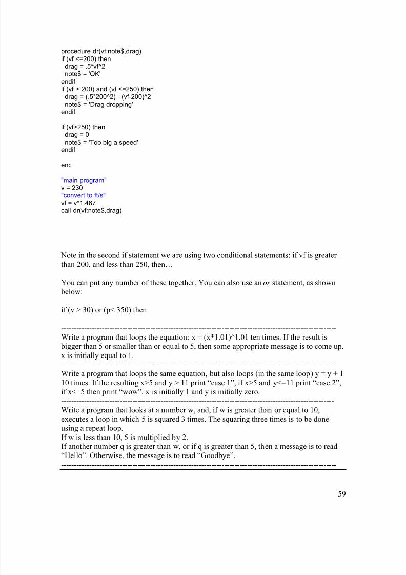
8/6/2019 Practical Computing for Engineers-V1
http://slidepdf.com/reader/full/practical-computing-for-engineers-v1 59/119
59
procedure dr(vf:note$,drag)if (vf <=200) then
drag = .5*vf^2note$ = 'OK'
endif if (vf > 200) and (vf <=250) then
drag = (.5*200^2) - (vf-200)^2note$ = 'Drag dropping'
endif
if (vf>250) thendrag = 0note$ = 'Too big a speed'
endif
end
"main program" v = 230"convert to ft/s"
vf = v*1.467call dr(vf:note$,drag)
Note in the second if statement we are using two conditional statements: if vf is greater than 200, and less than 250, then…
You can put any number of these together. You can also use an or statement, as shown below:
if (v > 30) or (p< 350) then
------------------------------------------------------------------------------------------------------------Write a program that loops the equation: x = (x*1.01)^1.01 ten times. If the result is bigger than 5 or smaller than or equal to 5, then some appropriate message is to come up.x is initially equal to 1.------------------------------------------------------------------------------------------------------------Write a program that loops the same equation, but also loops (in the same loop) y = y + 110 times. If the resulting x>5 and y > 11 print “case 1”, if x>5 and y<=11 print “case 2”,if x<=5 then print “wow”. x is initially 1 and y is initially zero.
-----------------------------------------------------------------------------------------------------------Write a program that looks at a number w, and, if w is greater than or equal to 10,executes a loop in which 5 is squared 3 times. The squaring three times is to be doneusing a repeat loop.If w is less than 10, 5 is multiplied by 2.If another number q is greater than w, or if q is greater than 5, then a message is to read“Hello”. Otherwise, the message is to read “Goodbye”.------------------------------------------------------------------------------------------------------------

8/6/2019 Practical Computing for Engineers-V1
http://slidepdf.com/reader/full/practical-computing-for-engineers-v1 60/119

8/6/2019 Practical Computing for Engineers-V1
http://slidepdf.com/reader/full/practical-computing-for-engineers-v1 61/119
61
time = time + deltat "elapsed time" i = i + 1
until (i = 11)end
"main program" deltat = 0.1 "time steps in seconds" mass = 100 "mass in kg" call termvel(deltat,mass:time,v[1..10])
Let’s look at this program step-by-step, starting with the main program at the bottom.
The main program defines the time step deltat and the mass, then calls procedure termvel. Notice that it passes inputs deltat, and mass to the procedure, and specifies that time andv[1..10] will be the outputs. v[1..10] means that we are instructing EES to display in our solution velocities 1 through 10. We could have written just, say v[4], and then only v[4]would have been displayed.
Procedure termvel at the top of the program is first given the initial value of v=0 at timestep one (v[1] = 0). We initialize the time as zero, just as the previous program, and begin a counter i.
Now comes the part that might “throw you for a loop”. Inside the loop, notice the line:
v [i+1]= (500 - .07*v[i]^2)*deltat/mass + v [i] [1]
Recall that we are using the previous time step’s velocity to calculate the current timestep’s velocity. If i = 1 (the first time the loop is executed), then the equation above will
be understood by the computer as:
v [2]= (500 - .07*v[1]^2)*deltat/mass + v [1]
The second time the loop is repeated, counter i will equal 2, and the computer willunderstand equation [1] as:
v [3]= (500 - .07*v[2]^2)*deltat/mass + v [2]
Do you see what is happening? Thanks to the array, we have written one equation that isgood for all of the time steps, without having to write the equation out many, many times!In addition, we are storing v[1] through v[10].
At the end of each loop we update the counter by:
i = i + 1
And finally, the loop is instructed when to finish by the line
Until (i = 11)

8/6/2019 Practical Computing for Engineers-V1
http://slidepdf.com/reader/full/practical-computing-for-engineers-v1 62/119
62
This may seem confusing since we want the loop to be executed ten times, but notice thatin the statement before this one we are adding one to i, so the loop will have executed tentimes when i = 11.
When you run this program, the ten velocities will be displayed in the Arrays Window – after running the program, go to Windows/Arrays to see your solution.-----------------------------------------------------------------------------------------------------------Homework:
For flow between parallel plates, with one plate moving at u = 100 m/s and the other stationary, the velocity at any point is equal to the average of the velocities above and below it:
We then have the following 6 equations:
100
2/)(
2/)(
2/)(
2/)(
0
1
132
243
354
465
6
=
+=
+=
+=
+=
=
u
uuu
uuu
uuu
uuu
u
We need to solve these equations simultaneously. One way to do this is by Gauss-Seidel
iteration. To do this, you assign an initial value to all the u’s, say 1, and then just keeplooping through the equations. The equations will keep changing with each loop, untilthey stop changing known as convergence). When this happens, the simultaneousequations can be considered to have been solved. We will use arrays to keep track of eachu, and to only have to write the equation for u once.
u=100 m/s
Stationary Plate u = 0
y
2
3
4
5
6
1

8/6/2019 Practical Computing for Engineers-V1
http://slidepdf.com/reader/full/practical-computing-for-engineers-v1 63/119
63
Write a program to do the following (remember that all programming such as looping andconditional statement must be done in a procedure, and that the procedure must be calledfrom the main program at the bottom of the program)
a) Using arrays, set u(1) and u(6) to 1000 and 0, respectively.
b) Initialize all the u values (u(2) – u(5) to a value of 1.hint:i = 2repeatu(i) = 1i = i+1
until(i>5)
b) loop through the equations 100 times:u(i) = (u(i+1) + u(i-1) )/2
c) Print to the screen all the u values. Have the computer give you a warning if u(2) isgreater than 50.
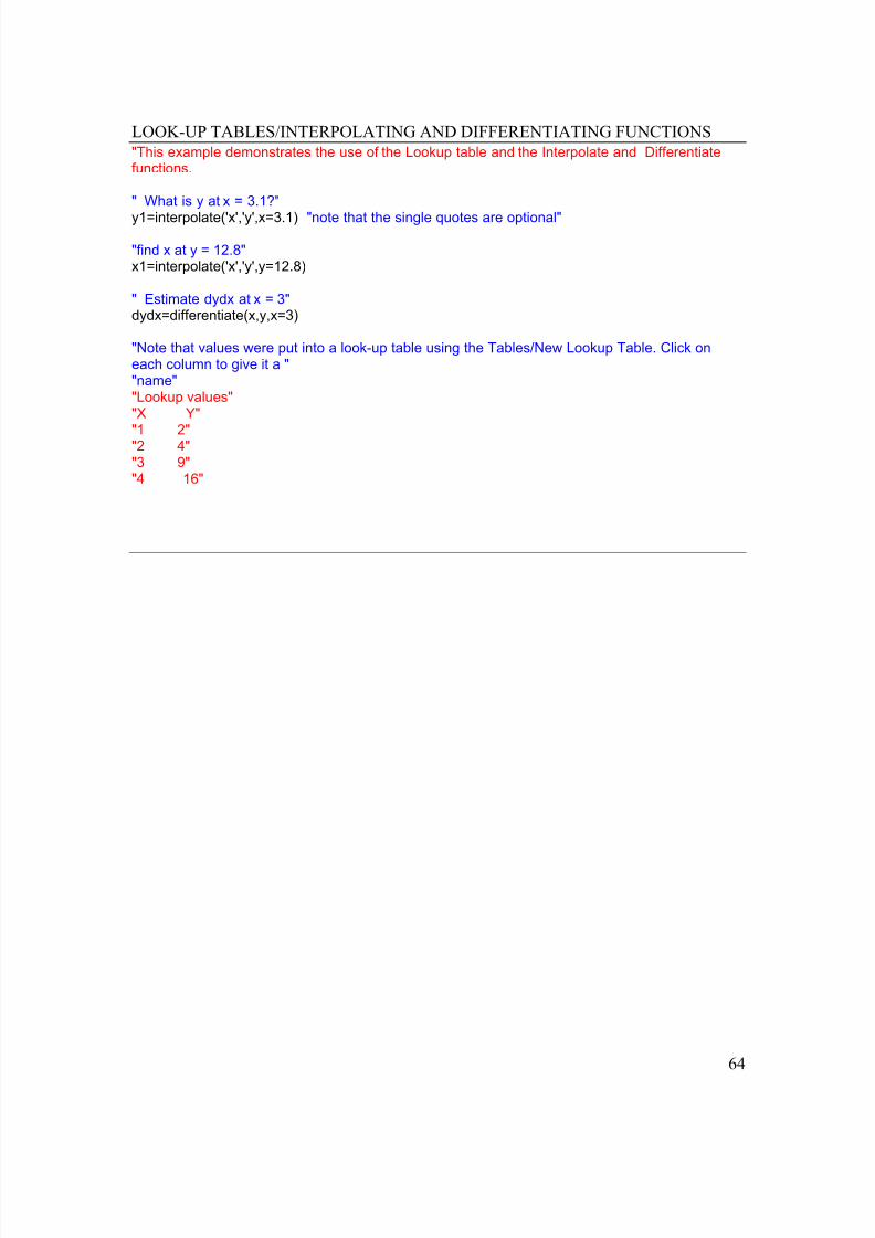
8/6/2019 Practical Computing for Engineers-V1
http://slidepdf.com/reader/full/practical-computing-for-engineers-v1 64/119
64
LOOK-UP TABLES/INTERPOLATING AND DIFFERENTIATING FUNCTIONS"This example demonstrates the use of the Lookup table and the Interpolate and Differentiatefunctions.
" What is y at x = 3.1?"
y1=interpolate('x','y',x=3.1) "note that the single quotes are optional"
"find x at y = 12.8" x1=interpolate('x','y',y=12.8)
" Estimate dydx at x = 3" dydx=differentiate(x,y,x=3)
"Note that values were put into a look-up table using the Tables/New Lookup Table. Click oneach column to give it a ""name""Lookup values""X Y"
"1 2""2 4""3 9""4 16"

8/6/2019 Practical Computing for Engineers-V1
http://slidepdf.com/reader/full/practical-computing-for-engineers-v1 65/119
65
CHAPTER 4: MATLAB
Matlab is a powerful engineering tool that allows you to program, and also has many
built-in functions to help engineers do their jobs more effectively. Matlab is becomingvery popular in academia and industry.
Symbolic Mathematics
Matlab has the capability of to do symbolic mathematics, that is, solve equations with
variables in them, such as 3/32 xdx x =∫ . This is a feature that sets Matlab apart from
many other software packages in use by engineers.
If you have not already done so, install the Matlab software on your computer byfollowing the instructions which appear when you load the disk. Choose the standardinstallation option.
Before you begin: use the same notation you as in other languages: +,-,*,/ and ^ for raising to a power. In addition, the standard hierarchy of operations applies.
We now explore some of the capabilities of the Matlab product:
a) Type in the following command, which tells Matlab that the expression within theapostrophe marks is a symbolic expression:
y = sym(‘x^3 – 2*y^2 + 3*a’) and hit the return key. The output on your screen is:
y = x^3 – 2*y^2 + 3*a
OK, that was not too hard. Now do the same for the following expressions:
ym x y x E
x x x D x
x xC
x B
x A
813432
101332
)105(
)5(
25
23
2
2
2
−++−=
−−+=+
−−=
−=
−=
Please note that Matlab will distinguish between “A” and “a” in the names of theexpressions above.

8/6/2019 Practical Computing for Engineers-V1
http://slidepdf.com/reader/full/practical-computing-for-engineers-v1 66/119
66
b) The command “ ezplot “ makes a plot of symbolic expressions. Here is the format:
ezplot(A,[xmin,ymin])
This expression plots equation A from xmin to ymin.
Try it for expression A, from -1 to 1. You should get the following plot
We will look at plotting more closely soon, but for now, typing in the followingcommands will give you a title and x,y labels:
title(‘plot’)xlabel(‘x’)ylabel(‘y’)
Make a plot for expression B.
Equations may be manipulated easily in Matlab. Here are some examples:
c) factor(A) the answer should be (x+5)(x-5)d) expand(B)e) simplify(C) in this case, the equation cannot be simplified further!f) factor(D)

8/6/2019 Practical Computing for Engineers-V1
http://slidepdf.com/reader/full/practical-computing-for-engineers-v1 67/119
67
The “simplify” function above gives only one result only. There may be others:
simple(C) gives several other attempts at simplification, and “ans” will be the shortestone.
g) Come up with a symbolic expression that is greatly simplified by the “simplify”command.

8/6/2019 Practical Computing for Engineers-V1
http://slidepdf.com/reader/full/practical-computing-for-engineers-v1 68/119
68
SOLVING SIMULTANEOUS EQUATIONS IN MATLAB:
You will probably encounter simultaneous equations in electrical engineering and heattransfer.
It is very simple to use Matlab for solving simultaneous equations – one advantage over the techniques used so far is that there is no need to tell Matlab the range of the solutions,nor where to start iterating . This is because Matlab uses matrix algebra to solvesimultaneous equations, as opposed to iterative schemes. Matlab should give you everysolution that exists – not just the ones within a specified range. It’s then up to you todecide which solutions are good or not.
Let’s say you have the following equations:
3212
023 2
=−
=−
y x
y x
We wish to find the solution, or solutions to these equations.
Type in:
s = solve(‘3*x-2*y^2’, ‘12*x-2*y=3’)
Press enter. Note that if an equation is equal to zero, there is no need to specify that it’sequal to zero, as in the first equation. Note that the second equation is not equal to zero,and the entire equation is written out.
The result tells you the size of the matrix of each answer.. pretty confusing and useless tous.
Now type in:
M = [s.x, s.y]
This instructs Matlab to give the solution for x and y from s, and to put the solution in amatrix called M. The result is:
4/38/3
2/16/1 −
=M
This means that x = 1/6 , y = -1/2 is one solution, and x=3/8, y = ¾ is another solution. Note that when you defined M, you told Matlab how to present the data to you. If youhad typed in M = [s.y, s.x] the solution would have been:

8/6/2019 Practical Computing for Engineers-V1
http://slidepdf.com/reader/full/practical-computing-for-engineers-v1 69/119
69
8/34/3
6/12/1−=M
These fractions are a little annoying, so we get rid of them by typing in:
vpa(M, 5), which gives you 5 digits in the answer:
75000.37500.
50000.16667. −=M
Try solving the following equations:
y x z
y z x
z y x
65
26
5210 3
+−=
=−
=+
The solution matrix for x, y, z is (using 4 digits):
320.2198.1973.
320.2198.1973.
000
−−−
=M
In other words, x = 0, y = 0, z = 0 is one solution. x = .973, y = 1.198, z=2.320 is another,etc.
Solve the simultaneous equation solved earlier:
Qtotal = 1.712E-9 * (1000^4 – T1^4) + 5* ( 90 – T1)
Qtotal = 100*(T1 – T2)
Qtotal = 25 *(T2 – 30)
There will be four solutions: one will have negative temperatures, and two others willhave “unreal” solutions with the number “i”. The solutions should be q = 1712, t1 =115.6 and T2=98.47, using 4 digits in the vpa command.
We note that it appears that this procedure is the easiest so far s compared with Excel andEES, once the syntax has been learned.

8/6/2019 Practical Computing for Engineers-V1
http://slidepdf.com/reader/full/practical-computing-for-engineers-v1 70/119
70
DIFFERENTIATION AND INTEGRATION. M FILES.
Taking derivatives and performing integration are very simple with Matlab, but beforewe do that, it’s a good time to talk about M-files.
Have you noticed that we seem to be able to put in only one Matlab command at a time atthe EDU prompt? We would like to write longer sets of instructions – that is, we will bewriting programs. Programs in Matlab are known as M-files. M-files allow you to write aseries of instructions, not just one instruction at the prompt, as we have been doing.
Making an M-file is simplicity itself. Go up to File/New/M-file on the upper left corner of your screen, and click on the M-file. A blank screen will appear in which you can typein your commands. Type in the following:
% Note the % character is for making comments sa= sym('6*x^3 - 4*x^2+b*x') sb=sym('sin(a)'); %semi-colon is there to suppress printing "sin(a)"
%on the screen when the program runs. sc=sym('(1-x^3)/(1+x^4)')
%syntax for differentiating sa twice is: diff(sa,'x',2) % sa is the symbolic expression to differentiate, 'x' is the variable
with % respect to which differentiation is done, and 2 is the number of
times to % take derivative. sadif=diff(sa,'x',1) sadif2=diff(sa,'x',2) sbdif=diff(sb) %leave out the extra parameters and it does 1st
derivative
% wrt variable closest to letter "x". In this case there % is only one variable, a scdiff=diff(sc)
Run it by hitting the F5 key. To see the output, return to the main window, which should be accessible on the upper or lower edges of your screen. You will see the answers:
sa = 6*x^3 - 4*x^2+b*x
sc =(1-x^3)/(1+x^4)
sadif = 18*x^2-8*x+b
sadif2 = 36*x-8
sbdif = cos(a)
scdiff =-3*x^2/(1+x^4)-4*(1-x^3)/(1+x^4)^2*x^3

8/6/2019 Practical Computing for Engineers-V1
http://slidepdf.com/reader/full/practical-computing-for-engineers-v1 71/119
71
Notice that the expression for sb was not printed in the output. This is because wesuppressed it by using the semi-colon. There are times, especially when you may havevery long expressions, that you will want to do this.
The last expression looks complicated. Maybe we can simplify it. Add the linesimplify(scdiff) to your program:
ans = x^2*(-3+x^4-4*x)/(1+x^4)^2
You can also make it easier to look at by using the pretty command:
pretty(ans)
Here’s the output:
2 4x (-3 + x - 4 x)------------------
4 2(1 + x )
Next let’s try integration. Let’s modify the old program to avoid typing in morecharacters.
% Note the names sa, sb and sc are not magical! % just about any name will do - cannot start with a number
sa= sym('6*x^3 - 4*x^2+b*x') sb=sym('sin(a)') sc=sym('(1-x^3)/(1+x^4)')
%syntax for integration is int(sa,'x') % sa is the symbolic expression to differentiate, 'x' is the variable
% with respect to which integration is done saint=int(sa,'x') sbint=int(sb,'a') scint=int(sc,'x',1,3) %definite integral from 1 to 3 wrt x
scintsimpler=simplify(scint)
Here’s the output (Note that sb is no longer suppressed, and that the final equationappears to be in its “simplest” form before the simplify command!)
sa = 6*x^3 - 4*x^2+b*x
sb = sin(a)
sc = (1-x^3)/(1+x^4)

8/6/2019 Practical Computing for Engineers-V1
http://slidepdf.com/reader/full/practical-computing-for-engineers-v1 72/119

8/6/2019 Practical Computing for Engineers-V1
http://slidepdf.com/reader/full/practical-computing-for-engineers-v1 73/119
73
SOLVING DIFFERENTIAL EQUATIONS WITH MATLAB. FUNCTIONS. MOREPLOTTING.
Matlab has the capability to solve complex differential equations, far in excess of EES.Let’s start with the differential equation we have come to know so well, for a fallingobject subject to a drag force. You will recall that it’s an ordinary differential equation,and that we solved this using Euler’s method before, by marching forward in time:
dt mdV V /2^07.500 =−
We wish to solve this using an intial value of V = 0, and we wish to know the speed V asa function of time.
In order to do this, we must fist learn how to use functions. A function is a program you
write that you will call from another program. It’s similar to a procedure in EES. Let’smake a function that converts degrees to radians. We first make an M-file that will call afunction called DegtoRad. Note we will be passing the value of degrees to the function,and that we do not need to specify what the output will be. Name it anything you like:
%program to call a function called DegtoRad %which converts degrees to radians degrees = 15 radians = DegtoRad(degrees)
Now we actually define the function. Make another M-file and make sure you save itusing the name of the function, which in this case is DegtoRad
%illustrates use of a function to make a %calculation. It's very important that the %function name DegtoRad is the name under %which M-file is saved. function output=DegtoRad(x) output=x*pi/180;
Just run the main program by hitting F5, while in the main program. Your output should be:
degrees = 15
radians = 0.2618
Functions are not just for solving differential equations. They can be very useful in thatyou could write a function that you could call from any other program, without having tore-write what’s in the function.------------------------------------------------------------------------------------------------------------ProblemWrite a function that converts from Centigrade to Fahrenheit

8/6/2019 Practical Computing for Engineers-V1
http://slidepdf.com/reader/full/practical-computing-for-engineers-v1 74/119
74
------------------------------------------------------------------------------------------------------------
Now that you know how to use a function, we can continue with our differential equationequation:
dt mdV V /2^07.500 =−
Recall that the mass is 100, and that the initial velocity at time zero is zero.
We will be using a pre-made (it comes with Matlab) differential equation solver, ode45,which solves initial value problems like ours, in a similar way to the programs you have been writing to use Euler’s method. You will need two M-files: one to define the problem, and a function that ode45 will access.
Following is the first M-file. The differential equation is for dV/dt, so the variables are tand v:
%for solving a d.e.
[t,v] = ode45('termvel',[0,156],0) %termvel is the name of the function
%that the function ode45 will be
%calling. The equation will be
%evaluated from t= 0 to t = 156 (in
%the brackets), and the initial
%value of the velocity is zero.
plot(t,v) %let’s plot it xlabel('time(s)') ylabel('velocity (m/s)')
The function which is used by the differential equation solver is then made. You mustsave it under the name of termvel (in this case)
function dydt=termvel(t,v) dydt=(500-.07*v^2)/100;
That’s all there is to it! Now go to the first program above and run it. Here’s the output plot:

8/6/2019 Practical Computing for Engineers-V1
http://slidepdf.com/reader/full/practical-computing-for-engineers-v1 75/119
75
The terminal velocity is about 85 m/s, based on the plot. The numerical output gives it atabout 84.5 m/s, which is what we had earlier.
You may notice that Matlab presents the numerical output in a rather annoying way: itlists all of the times, then the velocities. You can add the following line to your main
program:
table=[t,v]
to get the output in a table format, with t and v presented in columns. Please explore theHelp section for more detail, as there are other options you can use here. The next pagehas the output.

8/6/2019 Practical Computing for Engineers-V1
http://slidepdf.com/reader/full/practical-computing-for-engineers-v1 76/119
76
table =
0 00.0000 0.00010.0000 0.0001
0.0000 0.00020.0000 0.00020.0001 0.00050.0001 0.00070.0002 0.00100.0002 0.00120.0005 0.00250.0007 0.00370.0010 0.00500.0012 0.00620.0025 0.0125
0.0038 0.01880.0050 0.02510.0063 0.03130.0125 0.06270.0188 0.09410.0251 0.12550.0314 0.15690.0628 0.31390.0942 0.47090.1256 0.62790.1570 0.78490.3140 1.56970.4710 2.35420.6280 3.13840.7850 3.92201.5699 7.82712.3549 11.69883.1398 15.52113.9248 19.27887.1834 33.890710.4419 46.444213.7005 56.625216.9590 64.485019.1167 68.577221.2744 71.906423.4320 74.579825.5897 76.711427.7474 78.410329.9050 79.750732.0627 80.7986

8/6/2019 Practical Computing for Engineers-V1
http://slidepdf.com/reader/full/practical-computing-for-engineers-v1 77/119
77
34.2204 81.618536.9847 82.424839.7491 83.009742.5135 83.421845.2778 83.7182
48.4662 83.973651.6546 84.148154.8431 84.259258.0315 84.334161.9315 84.405465.8315 84.449669.7315 84.470673.6315 84.482877.5315 84.495681.4315 84.503685.3315 84.5073
89.2315 84.509593.1315 84.511897.0315 84.5133100.9315 84.5140104.8315 84.5144108.7315 84.5148112.6315 84.5150116.5315 84.5152120.4315 84.5152124.3315 84.5153128.2315 84.5154132.1315 84.5154136.0315 84.5154139.9315 84.5154143.8315 84.5154147.7315 84.5154151.6315 84.5154152.7236 84.5154153.8157 84.5154154.9079 84.5154156.0000 84.5154

8/6/2019 Practical Computing for Engineers-V1
http://slidepdf.com/reader/full/practical-computing-for-engineers-v1 78/119
78
If a solution cannot be obtained using ode45, there are other built-in differential equationsolvers in Matlab. You might try ode15s if ode45 does not work, or consult the Helpsection.
--------------------------------------------------------------------------------------------------------
Problem
Solve the equationt
yt
dt
dy 23 −= for t from 1 to 3.5, with y = 4.2 at t=1. Plot it, and
create a table to view the results.
Solution: y = 5.844 at t =3--------------------------------------------------------------------------------------------------------ProblemThe cooling of a ball initially at 400 F, placed in 70 degree F air is governed by thedifferential equation:
)70(12 −−= T dt dT
where the upper case T is temperature in degrees F, and the lower case t is time, in hours.Make a plot of the temperature of the ball for the first hour.---------------------------------------------------------------------------------------------------------ProblemA ball is shot upward from an underwater cannon, at 5 m/s. The drag force on the ball isgiven by the equation:
drag = 100 V^2
The ball has a mass of 1 kg, and a buoyant force (upwards) of 30 Newtons.
Make a plot of the velocity of the ball as a function of time, and find the terminal velocityof the ball.---------------------------------------------------------------------------------------------------------

8/6/2019 Practical Computing for Engineers-V1
http://slidepdf.com/reader/full/practical-computing-for-engineers-v1 79/119
79
Plotting with Matlab.
Matlab has the capability to do very sophisticated 2-D and 3-D plotting. We now look atsome of the plotting features. Please note that we are only looking at a few of the plottingfeatures. Readers needing more detail are encouraged to use the ‘Help’ section of the
software, which is very extensive.
One of the strengths of Matlab is its ability to work with matrices – in fact, the nameMatlab stands for Matrix Laboratory. Matlab is great for manipulating matrices, and wasdesigned to do so. Hence, many features of Matlab use a matrix format or language fromlinear algebra. You will see this as we go along.
An array is a list if numbers or symbols arranged in rows and columns. For example:
68
32
is a 2 x 2 matrix, with two rows and two columns.
The simplest array is one row, or one column. Rows move horizontally, while columnsmove vertically. A row is sometimes referred to as a vector .
OK, that’s enough about matrices for now. Type in the following M-file:
x=[1:1:10]; %creates values from 1 to 10 in steps of 1 %also, created a vector called x
y=[1,3,4,5,7,9,9,10,7,5]; %vector y with assigned values z=[2:2:20]; %vector z from 2 to 20 step 2
plot(x,y,x,z) %we plot y vs x, and z vs x on same plot title('1st plot') xlabel('Distance(m)') ylabel('Velocity(m/s)') grid on %put on a nice looking grid hold on %put one more plot on same graph
%note that we could have used the %1st plot statement, and just add %z,y to it. hold on tells %Matlab to use the same plot as before
plot(z,y)
Let’s see how we can make the plot look better. Modify the plot commands as follows:
plot(x,y,'r--',x,z,'y-') %we plot y vs x, and z vs x on same plot plot(z,y,'b:+')
You will see the plot now has different color lines, different line styles (dashed), and thelast plot has data markers.

8/6/2019 Practical Computing for Engineers-V1
http://slidepdf.com/reader/full/practical-computing-for-engineers-v1 80/119
80
Here’s how it works: after the list of data pair to plot (x,y in our case), you can have up to4 characters inside the apostrophe marks (there does not have to be four, but 4 is the max)designating the way in which the data are plot.
Color markers: c (cyan)
m (magenta)y, r, g, b ( you can figure these out! b for Blue)k (black)
Line type characters: - (solid line)-- (dashed line): (dotted line)-. (dash-dot)
Data markers: + o * x s (square) d (diamond)
Example: plot(x,y,’ks’) would plot a black line with square data points marked. There isno need to insert spaces between the markers, but they must all be within the apostrophes.
There are many more plotting features that you should explore on your own using ‘Help’,should you desire them. In particular, on the figure itself you will see a toolbar on whichyou can access features such as legends, fonts, etc.
Curve-Fitting
Matlab has some very powerful curve-fitting features. You have already seen curve-fitting in the Excel portion of this course. Again, we are interested in getting an equationto a line based on the values of data pair.
The easiest way to get a fit to a line in Matlab is to use a plot. Go to the plot you justcreated, and click on Tools/Basic Fitting. A window will appear on the upper left of your screen. You will see an arrow at the bottom. Click on the arrow to open up the secondhalf of the window. You should see the image below:

8/6/2019 Practical Computing for Engineers-V1
http://slidepdf.com/reader/full/practical-computing-for-engineers-v1 81/119
81
You will also notice that, on the graph, each plot is given a name on the plot.
Select the data1 set of data, and select the quadratic fit (A 2 nd degree polynomial; cubic is
third).
You will now see that the coefficients to your fit are expressed in the window:

8/6/2019 Practical Computing for Engineers-V1
http://slidepdf.com/reader/full/practical-computing-for-engineers-v1 82/119
82
The residuals indicate the “goodness” of the fit. Now look at the plot:

8/6/2019 Practical Computing for Engineers-V1
http://slidepdf.com/reader/full/practical-computing-for-engineers-v1 83/119
83
Notice that the fit through the data is presented as a light blue line, and that the fit extendsBEYOND the range of the data (the data for the data 1 set stop at x = 10). This is because
data set 3 goes to x = 20. Matlab draws the fit to the end of the graph.
You should now experiment changing the fit to 3rd, 4th and 5th degree polynomials. Thereally nice thing about Matlab is that you can instantly see the effects and compare eachfit.
Matlab also gives you the option to create a fit from the M-file. Please see the ‘Help’section for more details.----------------------------------------------------------------------------------------------------------Problem
Use your thermodynamic tables to make a plot of Pressure (y-axis) as a function of Temperature for the saturated steam tables. Make a fit to T as a function of P. Use adashed line for your plot, with data symbols. Label the axes and the plot.-----------------------------------------------------------------------------------------------------------Problem
Make a plot of Pressure P (y-axis) as a function of enthalpy h. Try to make a polynomialfit to P as a function of h.
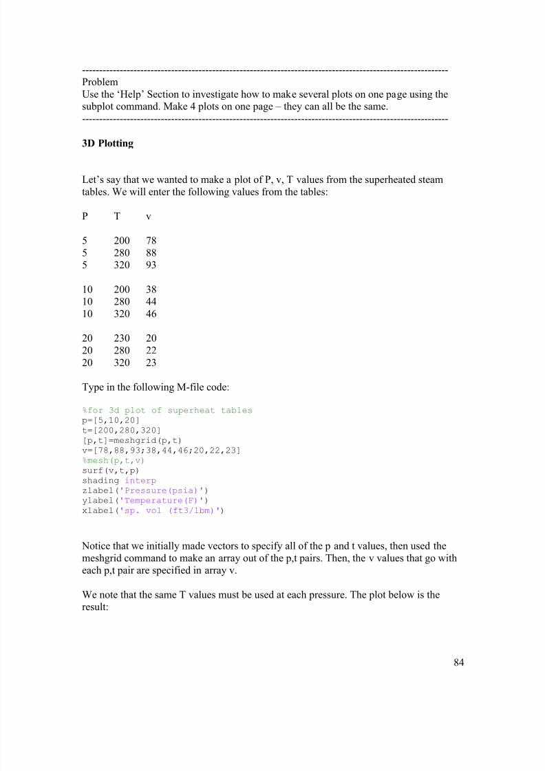
8/6/2019 Practical Computing for Engineers-V1
http://slidepdf.com/reader/full/practical-computing-for-engineers-v1 84/119
84
-----------------------------------------------------------------------------------------------------------ProblemUse the ‘Help’ Section to investigate how to make several plots on one page using thesubplot command. Make 4 plots on one page – they can all be the same.-----------------------------------------------------------------------------------------------------------
3D Plotting
Let’s say that we wanted to make a plot of P, v, T values from the superheated steamtables. We will enter the following values from the tables:
P T v
5 200 785 280 88
5 320 93
10 200 3810 280 4410 320 46
20 230 2020 280 2220 320 23
Type in the following M-file code:
%for 3d plot of superheat tables p=[5,10,20] t=[200,280,320] [p,t]=meshgrid(p,t) v=[78,88,93;38,44,46;20,22,23] %mesh(p,t,v) surf(v,t,p) shading interp zlabel('Pressure(psia)') ylabel('Temperature(F)') xlabel('sp. vol (ft3/lbm)')
Notice that we initially made vectors to specify all of the p and t values, then used themeshgrid command to make an array out of the p,t pairs. Then, the v values that go witheach p,t pair are specified in array v.
We note that the same T values must be used at each pressure. The plot below is theresult:

8/6/2019 Practical Computing for Engineers-V1
http://slidepdf.com/reader/full/practical-computing-for-engineers-v1 85/119
85

8/6/2019 Practical Computing for Engineers-V1
http://slidepdf.com/reader/full/practical-computing-for-engineers-v1 86/119
86
PROGRAMMING IN MATLAB
You can write extensive programs in Matlab M-files. Matlab has all of the programmingfeatures you have already seen, such as loops, conditional statements and arrays.
Looping is done using the ‘for’ statement, as shown in the code below:
%looping x=0; for i=1:2:10 % from one to ten in steps 2
x = x + 1 end % end closes a loop
Notice that when you run this code, x is printed on your screen each loop. We willsuppress the printing by using the semi-colon, and instruct Matlab to print the finalanswer:
%looping x=0; for i=1:2:10 % from one to ten in steps 2
x = x + 1; end % end closes a loop disp('x') %display the letter x disp(x) %display the value of x
There is also a formatted print statement, which allows you to print more than one result per line, and allows you to specify the number of characters to display.
x=0; for i=1:2:10 % from one to ten in steps 2 x = x + 1;
end % end closes a loop fprintf('\n x is %f',x) %fprintf('\n x is %f i is %f',x,i) %prints only a string (characters)
The \n tells Matlab to skip a line, while the ‘x is’ are characters you want printed. The %f tells Matlab to use notation with decimals for the x result. Try uncommenting the lastcommand and running it. It should print two results to the screen.
There are many more options for using the fprintf command. Please consult the ‘Help’
section of your software if you are interested.
It’s possible to put a loop within a loop, known as nested loops. Consider the code below:
%looping x=0; for i=1:2:10 %outer loop
for j=1:1:3 %inner loop

8/6/2019 Practical Computing for Engineers-V1
http://slidepdf.com/reader/full/practical-computing-for-engineers-v1 87/119
87
x = x + 1; end %closes the inner loop
end %closes the outer loop fprintf('\n x is %f',x) fprintf('\n') %to skip a line and get rid of EDU prompt
Run the code. Notice that there are two end statements, one for each loop. Incidentally,the indenting was done only to make it easier to see what’s going on.
Also notice that we put in an additional fprintf statement to skip a line, so the outputlooks better.-----------------------------------------------------------------------------------------------------------ProblemFor the commands:
for i=1:1:3 %outer loop
for j=1:1:4 %inner loop x = x + 1;
end %closes the inner loopend %closes the outer loop
What will be the final value of x, assuming it was 0 at the beginning of the program? Donot write a program to do this.----------------------------------------------------------------------------------------------------------ProblemWrite a program that will loop 100 times using the for command, using a counter toverify that the loop has indeed been done 100 times. Note that x is a counter in the codeabove.
----------------------------------------------------------------------------------------------------------ProblemWrite a program that loops 10 times in the outer loop and 5 times in the inner loop. Howmany iterations are done. Use a counter.-----------------------------------------------------------------------------------------------------------
SOLVING SIMULTANEOUS EQUATIONS WITH GAUSS-SEIDEL ITERATION
It’s possible to solve simultaneous equations by looping through them many times – atechnique known as Gauss-Seidel iteration. For example, consider the simultaneous
equations below:
2/23
2/)31(2
2/)2100(1
uu
uuu
uu
=
+=
+=
Let’s loop through them a few times and see what happens. We will set all the u values to1 at the beginning of our looping.

8/6/2019 Practical Computing for Engineers-V1
http://slidepdf.com/reader/full/practical-computing-for-engineers-v1 88/119
88
First loop:u1=(100+1)/2 = 50 %Note that we have a new value for u1 nowu2 = (50+1)/2 = 25.2 % we now have a new value for u2u3 = (25.2/2) = 12.75
2nd Loop:u1 = (100+25.2)/2 = 62.6u2 = (62.6+12.75)/2 = 37.675u3 = (37.65 /2) = 18.83
3rd loopu1 = (100+37.65)/2 = 68.85u2 = (68.85+18.83)/2 = 43.83u3 = (43.83/2) = 21.91
4
th
loopu1 = (100+43.83)/2 = 71.9u2 = (71.9+21.91)/2= 46.9u3 = (46.9/2) = 23.46
If we were continue this process for a while longer, we would eventually reach u1 = 75,u2= 50, u3 = 25. If you were to continue looping after this point, there would be nofurther change in the u values.
The technique we have just outlined is known as Gauss-Seidel iteration. It works as longas the equations are in the proper format, so that they satisfy the Scarborough criterion.The Scarborough criterion says that Gauss-Seidel iteration is guaranteed to converge if the following is true:
For all equations, the sum of the LHS coefficients divided by the sum of the RHScoefficients must be < = 1. For example, in the first equation, the sum of the leftcoefficients is 1, while the sum of the right coefficients is ½:
1st equation: 1/(1/2) = 2 Scarborough criterion not met!2nd equation: 1/(2/2) = 1 OK 3rd equation: 1/0.5 = 2 Scarborough criterion not met!
For at least one equation, the sum of the LHS coefficients divided by the sum of theRHS coefficients must be less than one. This is not met, either.
Gauss-Seidel iteration may still work if the Gauss-Seidel criterion is not met, but it’sguaranteed to work if the criterion is met.-------------------------------------------------------------------------------------------------------ProblemConsider the 4 equations:

8/6/2019 Practical Computing for Engineers-V1
http://slidepdf.com/reader/full/practical-computing-for-engineers-v1 89/119
89
x= 5 - y ; z = x + 6 – y ; q = 2 – y – 2x ; y = -2 – q – xCheck to see if they meet the Scarborough Criterion.(Sum of the coefficients for the lastequation: 1/(-1 + -1) = -0.5).
Loop through the equations using a calculator, and setting all the unknowns to 1 at the
beginning. Continue looping until there is no longer any change from loop to loop. Thefinal answers: x = 4, y = 1, z = 9, q = -7------------------------------------------------------------------------------------------------------------Write a Matlab program to loop through the equations 100 times (the number 100 is aguess that it will take fewer than 100 loops to solve this problem. The larger the number of equations, the larger the number of iterations required. Print the solution.------------------------------------------------------------------------------------------------------------Modify your Matlab program so that the value of the u2 is plotted as a function of thenumber of iterations. You may have to use the ‘hold on’ command.-----------------------------------------------------------------------------------------------------------
Conditional (If) Statements:
If statements are easy to implement in Matlab. Consider the following code, which alsoshows you how to input data from the program user:
hat = input ('Your hat size'); if hat >= 3
fprintf('You have a big head')
%else % fprintf('You have a small head ') end
You can see that this is very similar to the EES format. Note that every if statement must be closed with an end statement – everything between the if and the end is part of theconditional statement.---------------------------------------------------------------------------------------------------------ProblemActivate the commented (%) lines in the code above. You will see that the else statementis executed if the if statement does not apply.---------------------------------------------------------------------------------------------------------ProblemThe drag coefficient (cd) of a disc moving through the air is given by the values below.The cd vector is the drag coefficient, and the v vector is the velocity, from v = 10 to v =
40:
cd = [1.9,1.5,1.75,1.5]
V = [10,20,30,40]
From v = 40 to 90, the drag coefficient has different values:
cd2=[1.5,1.1,1.25,1.1,1,1] v2=[40,50,60,70,80,90]

8/6/2019 Practical Computing for Engineers-V1
http://slidepdf.com/reader/full/practical-computing-for-engineers-v1 90/119
90
Make a polynomial fit to Cd as a function of the velocity for the first set of data andanother for the second set of data. Write a program that inputs the speed from the program user. If the speed is greater than 90, then a message should say the velocity istoo great. For velocities between 0 and 90, the program should calculate the drag
coefficient, based on the right formula (As determined by the input speed).----------------------------------------------------------------------------------------------------------
“While” Loops
In EEs you encountered the repeat/until commands. You will recall that this involvedrunning a loop until a certain condition was met.
In Matlab you can perform loops until a condition is met using the “While” statement.Consider the code below:
% while-end loop x = 0; while x <=10
x = x+1; fprintf(' %4.0f', x)
end
You can pretty easily figure out what is going on – the loop is performed until x is greater than or equal to zero, and x is incremented by a value of one each loop.
Please note that every while loop must have an accompanying end statement.
------------------------------------------------------------------------------------------------------------ProblemWrite a Matlab program using a while loop that divides the number 100 by a value of two, until the result is less than or equal to 17. What is the final result, and how manyloops are performed. Your program must give the final answer and count the number of loops.------------------------------------------------------------------------------------------------------------ProblemWrite a Matlab program using a while-loop. The program is to start with the number 100,and is to divide it by 2. Next loop it is to divide the result by 2 again, and to repeat the
process until the change in the result from loop to loop is less than 0.25. For example:
1st loop: x = 50, change in x = 50Loop 2: x = 25, change in x = 25Loop 3: x = 12.5, change in x = 12.5
Here’s a program to do it:% while-end loop

8/6/2019 Practical Computing for Engineers-V1
http://slidepdf.com/reader/full/practical-computing-for-engineers-v1 91/119
91
x = 100; dif = 10000; % a safe value to make sure loop executes the first time xold = 1000; % a safe value to make sure loop continues on 1st loop while dif > 0.25 % loop executed while the difference between x values % w is less than 0.001
x = x/2 dif = abs(xold-x); xold = x; i = i+1; %a counter
end
disp('x') %disp is quick way to show answers or strings without
%formatting disp(x) %actual answer for x disp('') %print a space disp('i') disp(i)
------------------------------------------------------------------------------------------------------------Problem
Write a program that first adds 10 to 100, then 5 to the result (that is, 110+5) , then adds2.5 (115+2.5), and continues this pattern, until the change is less than 0.001. Display thefinal result, and count the number of loops executed.
The code below does it. You will need to understand it to do the next problem, or one of your own (there are many ways to solve most programming problems!):
% while-end loop dif = 10; % need this statement so loop will be satisfied first loop xold = 1000; % on first loop there is no xold yet, so pick a safe value x=100; % starting value to add to po = 20; % need this in first line in loop i = 0 while dif > 0.001 % loop executed while the difference between x values
% w is less than 0.001 x = x+po/2; %calculate x dif = abs(xold-x); %calculate abs value of difference between old
% and new x xold = x; %value of x juts calculated becomes xold po = po/2; %cut increment by one half i = i+1; %counter
end
disp('x') %disp is quick way to show answers or strings without%formatting disp(x) %actual answer for x disp('') %print a space disp('i') disp(i)
-----------------------------------------------------------
Problem

8/6/2019 Practical Computing for Engineers-V1
http://slidepdf.com/reader/full/practical-computing-for-engineers-v1 92/119
92
When we wrote the Gauss-Seidel program above, we assumed that 100 iterations weresufficient for the variables to stop changing from loop to loop. Write a program that performs Gauss-Seidel iteration on the same simultaneous equations used earlier in theGuass-Seidel section, but instead of using a for-loop that loops 100 times, use a while-loop that stops when the 3rd equation changes by less than 0.0001.
-----------------------------------------------------------------------------------------------------------
ProblemSolve the differential equation we have been using:
dt mdV V /2^07.500 =−
where m = 100, and V = 0 at t = 0. Loop through the equation until terminal velocity isreached, and display the value of the terminal velocity. Define terminal velocity asoccurring when the velocity changes less than 0.01 m/s per loop.-----------------------------------------------------------------------------------------------------------
Class ProjectMake a Matlab program to input Pressure in psia, and output the following: saturationtemperature (F and C), hf and hg (in BTU/lbm and kJ/kg), sf and sg (BTU/lbm-R andkJ/kg-K), vf and vg (ft^3/lbm a,d m^3/kg). Use a different function for each.
Input the U.S. units, and use conversion factors to calculate the SI values. Have the program tell you the units of each answer. The class will be broken up into groups, andeach group will fit a different property, after which all the data will be shared.
You may input every other value from the steam tables, as long as you include the lowestand highest value on the table.
Do this two ways:
1) using curve-fitting (if it is not possible to fit some of the data well, you may have to break it up into sets – for example, from 10-500 psia, and from 500-700 psia, etc.)
2) By having Matlab look at the values in a table, and interpolating between values.Matlab can automatically do this for you using the interp1 function (last letter in thenumber 1).
For example: say you had the following values for temperature and internal energy:
T= [100, 150, 200, 250, 300, 400, 500];u = [2507, 2583, 2658, 2734, 2810, 2968, 3132];
and you wanted to know the value of u that went with a temperature of T = 215. Here isthe code:
%for interpolating
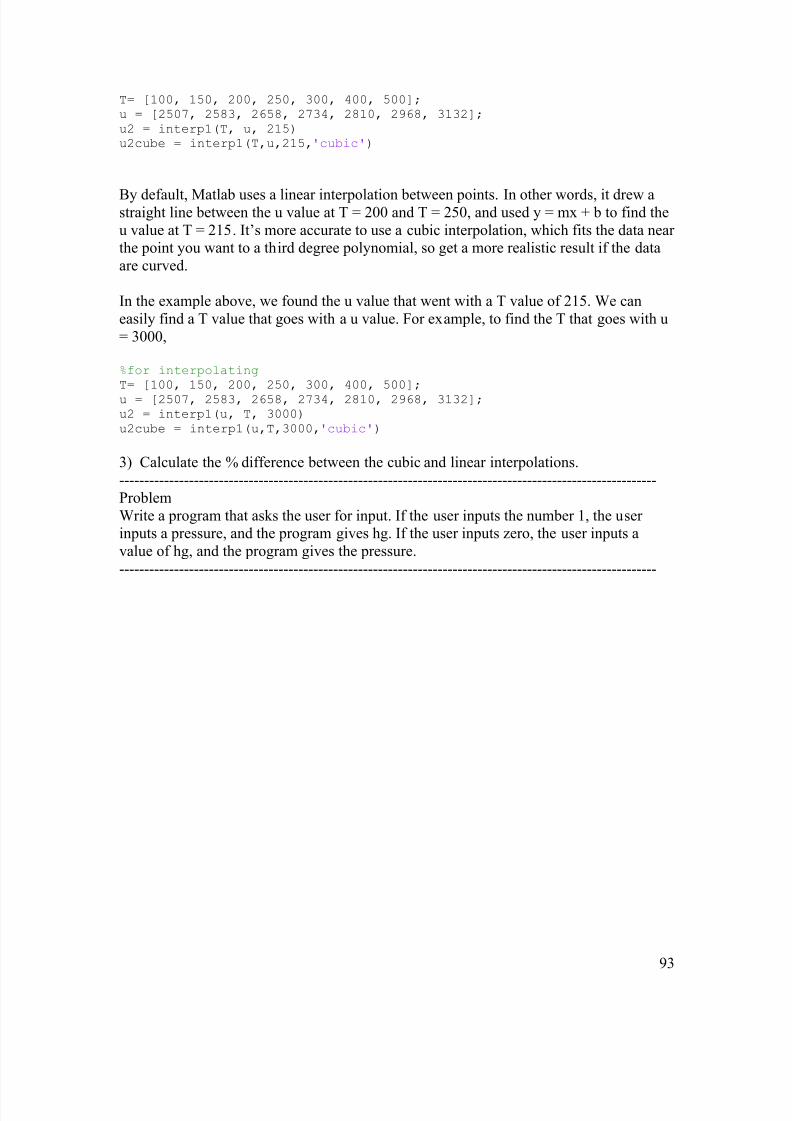
8/6/2019 Practical Computing for Engineers-V1
http://slidepdf.com/reader/full/practical-computing-for-engineers-v1 93/119
93
T= [100, 150, 200, 250, 300, 400, 500]; u = [2507, 2583, 2658, 2734, 2810, 2968, 3132]; u2 = interp1(T, u, 215) u2cube = interp1(T,u,215,'cubic')
By default, Matlab uses a linear interpolation between points. In other words, it drew astraight line between the u value at T = 200 and T = 250, and used y = mx + b to find theu value at T = 215. It’s more accurate to use a cubic interpolation, which fits the data near the point you want to a third degree polynomial, so get a more realistic result if the dataare curved.
In the example above, we found the u value that went with a T value of 215. We caneasily find a T value that goes with a u value. For example, to find the T that goes with u= 3000,
%for interpolating T= [100, 150, 200, 250, 300, 400, 500]; u = [2507, 2583, 2658, 2734, 2810, 2968, 3132]; u2 = interp1(u, T, 3000) u2cube = interp1(u,T,3000,'cubic')
3) Calculate the % difference between the cubic and linear interpolations.------------------------------------------------------------------------------------------------------------ProblemWrite a program that asks the user for input. If the user inputs the number 1, the user inputs a pressure, and the program gives hg. If the user inputs zero, the user inputs avalue of hg, and the program gives the pressure.------------------------------------------------------------------------------------------------------------
8/6/2019 Practical Computing for Engineers-V1
http://slidepdf.com/reader/full/practical-computing-for-engineers-v1 94/119
94
Automatic Data Acquisition Using Matlab
Suppose that you were running an experiment, where you wanted to determine the strain(stretch) on a beam as a function of the load on the beam, and that you wanted the resultsof the experiment (strain vs. load values) to automatically go into your computer.
In the old days, you might have had some type of analog output: you’d probably read theneedle on a gauge, and the gauge would be calibrated to show strain. You would thenhave to enter the values in a notebook, and plot the data on a graph by hand.
To run an experiment and have the data go directly into your computer you need thefollowing:
1) A sensor that changes voltage or resistance as the experimental phenomenon you want
to measure changes.
For example, say you are measuring the strain on a beam, a strain gauge pasted on thesurface of the beam changes electrical resistance as the beam stretches or compresses.The change in resistance of the gauge can then be calibrated to indicate strain. For example, a 10 micro-ohm change indicates a strain of 0.001, etc.
If you were running a fluid flow experiment in which you were interested in measuringthe speed of some water flow, you might have the current turning a small electricgenerator, and the amperage of the resulting current could be calibrated to indicate thespeed of the current.
The two examples listed above give analog outputs, that is, outputs that are changingcontinuously and smoothly with time. Computers work digitally – they require the outputfrom the experiment to be discrete (non-continuous) values made up of ones and zeroes.
2) A way to convert the analog output of your measuring device to digital output that thecomputer can process.
This is done using an analog-to-digital (AD) converter. You can purchase these or buildyour own. Matlab is configured to easily accept measuring instruments and ADconverters from the following companies:
Measurement Computing Corporation National InstrumentsKeithley InstrumentsAdvantechVXI Technology
In addition, you can program Matlab to accept other designs, including your own, but thisis more involved.

8/6/2019 Practical Computing for Engineers-V1
http://slidepdf.com/reader/full/practical-computing-for-engineers-v1 95/119
95
AD converters typically require the output from the sensor to the AD converter to be avoltage between a certain range. This might require some circuits to step down or up thevoltage entering the AD converter.
In addition, the output from the sensor may be a resistance that is changing, which then
needs to be converted into a voltage that is changing. For example, a thermistor is aresistor affected by heat, used as a thermometer. In this case, a voltage divider must beused to convert the changing resistance into a changing voltage. The circuit belowillustrates a voltage divider:
Vout will then vary as R1 (the sensor) varies in resistance. The rule for determining theoutput voltage based on V1, R1 and R2 is:
12
2
R R
RVinVout
+=
3) A program to process the ones and zeroes it gets from the AD converter, and convert
them into meaningful output. For example, Matlab can process the data gathered during
a load-deflection experiment, and present to you a graphical output with deflection vs.load, as well as tabulated values of the data.
It should be noted that any measurement instrument needs to be calibrated – the changingcurrent or voltage must be translated into a force, pressure, flow rate, etc. If you purchasea ready-made package from one of the companies, this is probably already done for you, but it’s always a good idea to check the calibration vs. a known quantity.
R1(Sensor): a varying
resistance
R2 Vout
Vin
+

8/6/2019 Practical Computing for Engineers-V1
http://slidepdf.com/reader/full/practical-computing-for-engineers-v1 96/119
96
Incidentally, you do not necessarily need Matlab to do automatic data acquisition. Thecompanies that make the AD converters and data acquisition systems may have their ownsoftware to process the data. The benefit to using Matlab is in the many features it hasavailable for the processing of acquired data.------------------------------------------------------------------------------------------------------------
ProblemA therrmistor has a resistance of 10 ohms, inside a voltage divider circuit. Determinewhat size resistor is required for R2 if the AD converter needs voltage from 0.1 to 5 volts,and the voltage being supplied is 9V.------------------------------------------------------------------------------------------------------------ProblemSensors need to be calibrated using known values. In this problem you will use knownload values and corresponding voltage readings to determine the relationship betweenvoltage and the load.A strain gauge is connected to a computer, and we wish to calibrate it. The followingreadings are obtained from known loads:
Load: 1000 2000 3000 4000Voltage: 0.1 0.2 0.3 0.42
In order to calibrate the instrument, come up with a polynomial for the load, as a functionof voltage, which can be later used to determine the load, given the voltage.------------------------------------------------------------------------------------------------------------
Sample Rate:
The number of times per second that the AD converter acquires readings from the sensor is called the sample rate. It’s important to pay close attention to the sample rate to ensureyou get meaningful data.
For example, say that you are measuring the strain on a specimen being gradually loadedwith more and more weight. If the weight is being applied at a rate of 100 N/s, and youwere interested in capturing increments of 10 N, then the sample rate would need to be atleast 10 samples per second.
Some phenomena need to be sampled very quickly in order to capture them properly.One example of this is the acquisition of sound. As you know, sound has a frequency,expressed as cycles per second, or hertz (Hz). For example, striking a tuning fork set to1000 Hz will cause it to vibrate 1000 times per second.
Consider the plot below, showing how a 20 Hz signal might look (plot in green). Also onthe plot are some black squares, which show the data which would be gathered if sampleswere taken every 0.1 seconds. The black curve is the curve you might sketch in-betweenthe black squares.

8/6/2019 Practical Computing for Engineers-V1
http://slidepdf.com/reader/full/practical-computing-for-engineers-v1 97/119
97
You can see that the black curve is nothing like the real green curve, and that to capturethe real curve, one might need a sample rate of at least 40 samples per second (twice thefrequency of the sound).
This form of error, where the sample rate is not fast enough and results in a false
frequency is known as alias error .
Automatic Data Acquisition Example 1:
Using the soundcard, we can bypass steps 1 and 2 above for a simple demonstration of Matlab’s ability to acquire analog data.

8/6/2019 Practical Computing for Engineers-V1
http://slidepdf.com/reader/full/practical-computing-for-engineers-v1 98/119
98
The microphone on your computer is connected to a sound card that converts the analogsignal from the microphone into a digital signal that the computer can understand. Wethen have a sensor (the microphone) and the AD converter already in-place. If you do nothave the Automatic Data Acquisition Toolbox, you will not be able to perform this
experiment, but you should understand all the steps anyway.
Study and understand the Matlab code below:
%PROGRAM FOR USING SOUND CARD FOR ANALOG INPUT
% first instruct Matlab to receive analog data from the sound card % note that analoginput is a built-in function, and 'winsound' % is the sound card.
AI = analoginput('winsound')
%there are two channels available in the sound card. We will use %the first channel: addchannel(AI,1)
%next we specify the sample rate per second. Note that %8000 samples /s is the slowest the sound card samples %Note SampleRate must be spelled exactly sr = 8000; set(AI,'SampleRate',sr)
%specify how long we want to take samples for (s) howlong = 2;
%note SamplesPerTrigger must be spelled exactly. %It's the number of samples taken every time the program %runs (triggers the software). set(AI,'SamplesPerTrigger',howlong*sr)
%start taking data start(AI) data = getdata(AI) %the data will be pairs of time,Voltage plot(data)
save sound1.dat data – ascii %data saved in sound1.dat, in ascii format
%ascii format is readable by other programs
%close things up delete(AI)
That’s all there is to it! Using AD converters from the supported manufacturers is just aseasy. For example, to acquire data from National Instruments Hardware, you wouldchange the first command:
AI = analoginput(‘nidaq’,1)addchannel(AI,1)

8/6/2019 Practical Computing for Engineers-V1
http://slidepdf.com/reader/full/practical-computing-for-engineers-v1 99/119
99
or for Measurement Computing Corporation:
AI=analoginput(‘mcc’,8)addchannel(AI,1)
The number after the company abbreviation is hardware specific – companies havespecific numbers.
Consult the Matlab ‘Help’ and web site for more information on procedures to follow for automatic data acquisition.------------------------------------------------------------------------------------------------------------Problem/Project
This project will involve calibrating sound levels. Using Matlab, you will read soundsmade with your voice recorder, and use these sounds to write another Matlab programthat will determine if sounds are loud or soft, and give a value for the intensity of the
sound. You will not need the data acquisition toolbox, since the microphone’s sound will be recorded, and the resulting .wav file read using Matlab.
The code below reads a .wav file called sountest.wav. The values are for amplitude of thesound wave (sound looks like a sine wave – physically, it’s a series of high and low pressure pulses. Your computer is displaying amplitude values of the wave between +1and -1).
Make a .wav sound file using your computer’s sound recorder (no need to make it longer than about a second – you will be sampling data at a very fast rate, and even one secondwill give you thousands of readings), and call it sountest1 – make sure you save it inyour Matlab “work” directory. Run the program below and study the code carefully.
%for reading a .wav file[y,Fs]=wavread('sountest1',100); % y is the amplitude, between 1 and -1.
%Fs is the sample rate%the file is sountest1.wav, and the%first 100 samples are read only
fprintf('\n Sample Rate %f',Fs)x=[1:1:100]; %make some x points to go with y values, so we can plot plot(x,y)z=std(y); %std deviation of amplitude valuesc=max(y); %c is the max value of the datad=min(y); %min is the min value of the datafprintf('\n Std deviation %f',z)fprintf('\n Max amplitude %f',c)fprintf('\n Min amplitude %f',d)
The project involves two steps: calibration and software development

8/6/2019 Practical Computing for Engineers-V1
http://slidepdf.com/reader/full/practical-computing-for-engineers-v1 100/119
100
Calibration:Make two sound recordings – one whistling softly, and another whistling loudly (again,roughly one second is enough). Once these recordings are made, study their characteristics using the program above (it will need some modification – the samplesread are probably too few – you will need to determine about how many you need by
studying the data), and come up with a way in which you can distinguish loud whistlesfrom soft whistles, using the data. Come up with a linear scale from 1 to 100, where 1 isthe sound level of your soft whistle, and 100 is the loud whistle.
Software DevelopmentCome up with a Matlab program that will read a .wav file, and determine if the sound isloud or soft, assigning it a value from 1 to 100, based on your calibration above.-----------------------------------------------------------------------------------------------------------Fourier Transforms
Sound data, and many other forms of data, are plagued by unwanted signals referred to as
“noise”. For example, microphones can introduce a background hiss that should not be present. Data acquired could thus be composed of the desired signal as well as unwantednoise. This is not limited to the collection of sound data – you may run into this in other data collection schemes.
Consider for example the following pure 50 Hz simulated signal

8/6/2019 Practical Computing for Engineers-V1
http://slidepdf.com/reader/full/practical-computing-for-engineers-v1 101/119
101
The plot above is made with the following Matlab program:
%generates 50 Hz signal %the time points are made. They go up to 0.6 s.
%One every 0.001 s - a 1000 Hz signal. t = 0:0.001:0.6; %next we generate a wave of 50 cycles for every one t x = sin(2*pi*50*t)
plot(1000*t(1:50),x(1:50)) %we plot only the first 50 points title('50 Hz pure signal') xlabel('time (milliseconds)')
Now we wish to corrupt the signal with some noise. We will do this using a randomnumber generator in Matlab. Consider the code below:
%demonstrates fft %the time points are made. They go up to 0.6 s. %One every 0.001 s - a 1000 Hz signal. t = 0:0.001:0.6; %next we generate a wave of 50 cycles for every one t x = sin(2*pi*50*t)
y = x + 2*randn(size(t)); %add some random noise to it plot(1000*t(1:50),y(1:50)) %we plot only the first 50 points title('50 Hz corrupted signal') xlabel('time (milliseconds)')

8/6/2019 Practical Computing for Engineers-V1
http://slidepdf.com/reader/full/practical-computing-for-engineers-v1 102/119
102
The result is the plot below:
If you compare this with the original plot, you can see that you would be hard-pressed tolook at the corrupted signal and know that it came from the 50 Hz signal!
Here’s where Fourier transforms can help out. Any cyclic data (wave-like), such assound, can be represented by equations using consisting of sine waves of variousfrequencies, known as Fourier transforms. Without getting into some very complicateddetails, Matlab can do this using the fft function, which stands for Fast Fourier Transform(FFT). The Fast Fourier Transform is a very efficient way of performing Fourier transforms.
When performing FFT, you must specify the number of points used, and they must be a
power of 2. For example, 32, 64, 128, 256, 512, etc are valid. The more points used, themore frequencies can be detected.
%demonstrates fft t = 0:0.001:0.6; x = sin(2*pi*50*t)
y = x + 2*randn(size(t));
Y = fft(y,512); %perform fast Fourier transform (FFT)

8/6/2019 Practical Computing for Engineers-V1
http://slidepdf.com/reader/full/practical-computing-for-engineers-v1 103/119
103
%The power spectrum, a measurement of the power at various frequencies,
%is given by the equation below Pyy = Y.* conj(Y) / 512;
%Graph the first 257 points (plotting all 512 is unnecessary)
% on a meaningful frequency axis. You could get this by trial
% and error f = 1000*(0:256)/512;
plot(f,Pyy(1:257)) title('Frequency content of y') xlabel('frequency (Hz)')
From the plot you can see that the most “power” is in the 50 Hz signal, meaning that themost significant signals are those in the 50Hz range.
Signals can be made up of more than one frequency. The code below will generate asignal made up of a 50 Hz and a 120 Hz signal. Notice we have simply modified the previous code where x is generated:
%generates 50 Hz with 120 Hz signal %the time points are made. They go up to 0.6 s. %One every 0.001 s - a 1000 Hz signal.

8/6/2019 Practical Computing for Engineers-V1
http://slidepdf.com/reader/full/practical-computing-for-engineers-v1 104/119
104
t = 0:0.001:0.6; %next we generate a wave of 50 cycles for every one t % x = sin(2*pi*50*t)
x = sin(2*pi*50*t)+sin(2*pi*120*t);plot(1000*t(1:50),x(1:50)) %we plot only the first 50 points title('50 Hz + 120 Hz pure signal') xlabel('time (milliseconds)')
The plot below shows what is looks like:
We now corrupt the data using a random number generator (the following code isessentially the same as code found in the help section of the documentation, under Fourier Transforms):
t = 0:0.001:0.6; x = sin(2*pi*50*t)+sin(2*pi*120*t); %corrupt it y = x + 2*randn(size(t)); Y = fft(y,512);
Pyy = Y.* conj(Y) / 512;
f = 1000*(0:256)/512; plot(f,Pyy(1:257))

8/6/2019 Practical Computing for Engineers-V1
http://slidepdf.com/reader/full/practical-computing-for-engineers-v1 105/119
105
title('Frequency content of y') xlabel('frequency (Hz)') plot(f,Pyy(1:257))
The figure below shows the plot:
Now we perform FFT using the code below:

8/6/2019 Practical Computing for Engineers-V1
http://slidepdf.com/reader/full/practical-computing-for-engineers-v1 106/119
106
The peaks at 50 and 120 can be clearly seen, representing the two frequencies making upthe signal.
----------------------------------------------------------------------------------------------------------Problem
Make a Fourier Transform of whistling noises of high and low pitches. Can you detectthe frequencies making up the sounds? How do they differ?---------------------------------------------------------------------------------------------------------

8/6/2019 Practical Computing for Engineers-V1
http://slidepdf.com/reader/full/practical-computing-for-engineers-v1 107/119
107
CHAPTER 6: OTHER COMPUTER LANGUAGES
Once you learn to program in one language, it becomes much easier to program inanother because many of the concepts are the same. We will look now at 3 other languages: C++, Java, Basic, and FORTRAN.
FORTRAN
FORTRAN language was very popular with engineers and scientists in the 1970s-1990s,and its popularity seems to be waning. It is still in use in some companies and institutions – some engineering colleges still teach it to its students. There are many, manysubroutines (similar to procedures and functions) which have already been written, andwhich you may need to access in your career. Knowing how to program in FORTRANcan be an asset for your advancement.
Please study the code below, which converts polar coordinates to rectangular coordinates
using a subroutine (a subroutine is like a procedure in EES, which is called to perform acertain procedure). The letter C denotes a comment, unprocessed by the computer. Alloperations must start on the 7th space.
C the next line specifies what type of numbers you will be working with.C variables rc, tc, xc, yc will be real numbers (with 8 digit accuracy, as opposed toC complex numbers, integers or double precision real numbers with16 digit accuracy)C The variable I will be an integer
REAL RC, TC, XC, YCINTEGER I
C The next line prints the statement in the apostrophe symbols. Note that you can giveC a number to a line in your program. The * denotes an unformatted input (you are notC specifying the way in which you want the statement displayed on the screen).
10 PRINT *,’Enter 2 Polar Coordinates, followed by 1 to go on, 0 to stop’
C Next we read in the values. The * denote unformatted input.C RC and TC are the polar coordinates we wish to convert
READ (*, *) RC, TC, I
C If I is ) the program will stop, otherwise it will continue
IF ( I .EQ. 0) THENGO TO 20END IF
C We call the subroutine to do the conversion. In the parentheses we must put what

8/6/2019 Practical Computing for Engineers-V1
http://slidepdf.com/reader/full/practical-computing-for-engineers-v1 108/119
108
C we are passing to the subroutine (polar coords RC and TC) and what the subroutineC will pass back to the main program ( rectangular coordinates XC and YC). TheC variables that you will pass back and forth are sometimes referred to as the arguments.
CALL CONVER(RC, TC, XC, YC)
C Print to the screenPRINT *,’Rectangular Coordinates’PRINT *, XC, YC
C Let’s put in a space in-between entries
PRINT *
C Go back to line 10
GO TO 10
20 END
C Here’s the subroutine
C Note that there are four variables next line. They correspond exactly to the variables inC the parentheses in the CALL statement above. In other words, RC corresponds to R,C TC to T, XC to X, and YC to Y. The reason for doing this is to enable the subroutineC to be used by any program, without having to change the names of the variables in theC subroutine.
REAL R, T, X, YX=R * COS(T)Y = R * SIN(T)END
Consider also the following FORTRAN commands (Not part of the program above),which you will readily decipher:
IF (X.GT.Y) THENGO TO 20END IF
And also the following code snippet, which loops 100 times, known as a DO Loop:
DO 40 I = 1, 100X = X + 1
40 CONTINUE

8/6/2019 Practical Computing for Engineers-V1
http://slidepdf.com/reader/full/practical-computing-for-engineers-v1 109/119
109
You may also run into the COMMON statement. Recall that when you used a subroutineyou had to have an argument list, which lists the variables which will be passed betweenthe main program and the subroutine. The arguments were in parentheses next to theCALL statement, and also on the first line in the subroutine.
Instead of listing the variables to be passed between main program and subroutines, aCOMMON statement is used instead. The COMMON statement puts the variables in asection of the computer’s memory that can be accessed by both subroutines and the main program, eliminating the need for the argument list. Consider the code below, which doesthe same as the previous program:
REAL RC, TC, XC, YCCOMMON RC, TC, XC, YCINTEGER I
10 PRINT *,’Enter 2 Polar Coordinates, followed by 1 to go on, 0 to stop’READ (*, *) RC, TC, I
IF ( I .EQ. 0) THENGO TO 20END IFCALL CONVER
C Print to the screenPRINT *,’Rectangular Coordinates’PRINT *, XC, YCPRINT *GO TO 10
20 END
C SubroutineREAL R, T, X, YCOMMON R, T, X, YX=R * COS(T)Y = R * SIN(T)END
Some other interesting (and at times quirky) facts about FORTRAN:
• The letters i, j, k, l, m, n are reserved for integers. For example, if you tried to setir = 6.7, you would encounter an error, since FORTRAN is expecting an integer.
• FORTAN must be compiled before running. After writing a FORTRAN program,say it was named flight1, you must type in a command such as fcomp flight 1(depending on the version of FORTRAN you are using). When you compile a

8/6/2019 Practical Computing for Engineers-V1
http://slidepdf.com/reader/full/practical-computing-for-engineers-v1 110/119
110
program, the program is converted into machine language, which is the formatyour computer understands. Compiled languages are typically faster than un-compiled languages.
• As mentioned earlier, program lines must begin on the 7th space.
• To use a subroutine not in your program, you may link to another program using
some form of link command, that might look something like: “ link flight1,conver”, which would link program flight1 with subroutine conver.
You may wonder why there is a need to distinguish between single and double precision(8 digits vs. 16) – why not use double precision all the time? The reason for this is thatoperations in double precision can take considerably longer to run. This may not be afactor for short calculations, but some programs need to run for millions of loops. In thiscase, a program might easily run over-night or longer.

8/6/2019 Practical Computing for Engineers-V1
http://slidepdf.com/reader/full/practical-computing-for-engineers-v1 111/119
111
Java
Java was created in the early 1990s, for use on the internet. It enables programmers tocreate applets, which are programs attached to web pages. These programs move across
the internet to computers accessing a web page with an applet installed.
The form you fill out when you purchase something on-line is probably written in Java,as may be any visual effects moving across your screen, or a game you play. Somescientists even use it for computations, as it has the features necessary for number-crunching, including loops, conditional statements, etc.
The difficulties in creating an internet computer language were numerous: it must work on any computer connected to the internet, it must not require any adjustments or installation of other software to run on other computers, and it must be safe from viruses.
An interesting thing about Java is that it is an open-source product. You can download itand use it for free from http://java.sun.com , or use any search engine to find it.
Here are some code snippets in Java. You can easily decipher them:
if (x >= 18) { p = 20*x;
}
Note the curly brackets show where the loop begins and ends.
Try this one:
for (int i=1; i<=5;I ++) {x = x+1;
}
The ‘int’ tells Java that the variable i is an integer. i will vary from a starting value of 1,and the loop will be executed as long as i is less than or equal to 5. The ++ indicates thatthe i will be incremented by one each loop.
Another sample:x = 0while (x<10) {x = x+1;
}
Like FORTRAN, after you write a Java program, you must compile it (translate it intomachine language).

8/6/2019 Practical Computing for Engineers-V1
http://slidepdf.com/reader/full/practical-computing-for-engineers-v1 112/119
112
Java is an object oriented language. You will hear this term a lot when dealing withcomputers. It refers to a language that enables programmers to use pre-made objects,which are procedures and data that are grouped together to perform complicatedoperations.
The author has found that object oriented programming, like entropy, can be quitedifficult to define. Typing ‘define object oriented programming’ into a search enginegives many results – most of them undecipherable.
Suffice it to say that object oriented programming makes writing complicated programsconsiderably easier.

8/6/2019 Practical Computing for Engineers-V1
http://slidepdf.com/reader/full/practical-computing-for-engineers-v1 113/119

8/6/2019 Practical Computing for Engineers-V1
http://slidepdf.com/reader/full/practical-computing-for-engineers-v1 114/119
114
// the file iostream is called a header file, because it usually goes at the head of the// program. The .h indicates it’s a header file.
using namespace std;/ * another format for the comment – the comment will finish at the next slash mark
followed by the asterisk.Visual C++ has what is called a standard library of functions useful to a programmer.There is a very large number of these, and the line above is put in to avoid problemswhich might arise if you use one of these names in your program. We end the commentwith the following */
void main( ){/* When you run a program, C++ needs to know where to start computing. Computationwill start after the curly bracket { . The end of the program will have another one}At times, you might see this statement as:
int main( ){
*/
int x = 1;double y = 25.4321678;float pi = 3.14159f;int z;
/* above are several types of variables in C++, and here are three of them. The first onedefines x as an integer, and assigns it a value of 1.The second one defines y as a double precision number, accurate to 15 decimal digits.The range of values stored is much wider than this – from 1.7 x 10^(-308) to 1.7 x10^(308), positive and negative, accurate to 15 digits.the third one defines a number with 7 digit accuracy, similar to the ‘real’ seen inFORTRAN.The last statement defines z as an integer, without giving it any valueALL VARIABLES MUST BE DEFINED IN C++ !! Note that program lines end with a semi-colon ;*/
if( x < 10){z = 15;}// you can figure the above out!
if(x = = 10)

8/6/2019 Practical Computing for Engineers-V1
http://slidepdf.com/reader/full/practical-computing-for-engineers-v1 115/119
115
{z = 20;}// you must use the double equal sign here, or else C++ will set x to 10
for ( i = 1; i < = 15; i++){sum = sum + 1;
}
/* The loop gets executed starting with i = 1, and continues as long as i is less than or equal to 15. i is incremented in steps of 1 (that’s what the ++ means). The curly bracketsdenote the beginning and end of the loop. Plese note that there is an error here, in thatvariables i and sum need to be defines at the beginning of the program, with statementslike int sum and int i */
while (x < 10){x = x + 1;}
/* you know this one! The expression for x could have been written as x++ to save 0.2seconds of typing. */
}/ / curly bracket ends main program
You should understand everything above.

8/6/2019 Practical Computing for Engineers-V1
http://slidepdf.com/reader/full/practical-computing-for-engineers-v1 116/119
116
APPENDIX TO DATA ACQUISITION SECTION
More data acquisition
The following M-file reads a temperature sensor. The output from the sensor/AD
converter is in Volts, between + and – 0.5 V. The purpose of the program is to calibratethe sensor – the known temperature will be input as the program runs, and then a plotmade of load vs. voltage. Once the relationship between temperature and voltage isknown, any future voltage readings can be converted to temperature. This program ismodified from a program found in the Matlab website, and is untested. There may beminor bugs.
% Thermistor Calibration
clear;
% Initialize Matlab Data Acquisition Engine
% The engine is set up to take one channel of analog input data,
% with a range between +/- 0.05 V.
%
% The sensor will be sampled at 1000 samples per second.
% 100 samples will be taken.
ai=analoginput('nidaq',1);
% (Creates analog input module called ai in Matlab)
chan=addchannel(ai,1);
% (Sets up Channel 1 for the thermistor output)
set(chan,'InputRange',[-.05 .05]);
% (Sets the range for channel 1). Note this was unspecified in the
% previous example.
set(ai,'samplerate',1000);
% (Sets the sample rate to 1000 samples/s)
set(ai,'samplespertrigger',100);
% (Causes the engine to take 100 samples when takes data)
set(ai,'BufferingConfig', [10 40]) % Set the bufferingConfig

8/6/2019 Practical Computing for Engineers-V1
http://slidepdf.com/reader/full/practical-computing-for-engineers-v1 117/119
117
%such that the product of the two numbers exceed samples per
%trigger. Data collected is stored in RAM, so must make room %for it in the buffer.
fle=input('\nEnter File Name for Saving Data: ','s');
% (User inputs file name to save test data)
%create figure (creates a window at the upper left of screen for plot)
set(0,'Units','pixels');
scnsize=get(0,'Screensize');
bdwidth=5;
topbdwidth=30;
pos1=[bdwidth,1/2*scnsize(4)+bdwidth,scnsize(3)/2-
2*bdwidth,scnsize(4)/2.5-(topbdwidth+bdwidth)];
figure('Position',pos1);
pause;
%open the file to receive the data
fid=fopen(fle,'w');%Opens file named in previous command
title=' "Thermistor Calibration" ';%This title will be placed in file
fprintf(fid,'%s\n',title);%Title is written to file
a='y';% Initialize variable a
i=0;%Initialize variable i
a='r';%Initialize the variable a
while a~='d'& a~='t' %This will allow program user to decide whether to
% keep taking data. If user presses d, program goes on, if enters t
% program ends. User will be prompted after each voltage, temperature
% reading is input.
a=input('\nEnter d to take Data, t to Terminate: ','s');
end;
%start the loop to take the data

8/6/2019 Practical Computing for Engineers-V1
http://slidepdf.com/reader/full/practical-computing-for-engineers-v1 118/119
118
while a=='d'
i=i+1;
start(ai);
% (Starts engine with immediate triggering
volt=getdata(ai); %Takes data from engine and puts in variable volt
temperature=input('\nEnter Weight on Load Cell: ');
% (Get user input of temperature being read)
w(i)=temperature;
vaves=mean(volt);%vaves is the average voltage reading
v(i)=1000*vaves;%v is load cell voltage in mV
%Print to Screen
display(['Temperature= ' num2str(w(i)) ' Cell
out(mV)='num2str(v(i))]);
%Show data on a plot
%create the plot
clf;%clears out the contents of the figure window
axes('position',[.3,.35,.5,.5]);%locates plot within window
hold;
plot(w,v,'*r');%puts data on plot
xlabel('Temperature','Fontsize',8);
ylabel('Thermistor Voltage - mV','Fontsize',8);
TITLE('Thermistor Output','Fontsize',9);
a='r';
while a~='d'& a~='t'
a=input('\nEnter d to take Data, t to Terminate: ','s');
end;

8/6/2019 Practical Computing for Engineers-V1
http://slidepdf.com/reader/full/practical-computing-for-engineers-v1 119/119
% (User decides whether to take more data)
end
title2=' temperature-(F) vldcl-(mV) ';%Column titles for output file
fprintf(fid,'%s\n',title2);%Print column titles to file
%print data to file
for j=1:i
fprintf(fid,'%8.4f',j,w(j),v(j));%Print test data to file
fprintf(fid,'\n');
end
fclose(fid);%close file