practical computing for biologists - duke universityccc14/pcfb/_downloads/...practical computing for...
TRANSCRIPT

Practical Computing for BiologistsRelease 1.0
Cliburn Chan
June 01, 2012


CONTENTS
1 Updates 1
2 Introduction 3
3 Course Description 5
4 Instructor: Cliburn Chan, Biostatistics and Bioinformatics. 74.1 Data Samples . . . . . . . . . . . . . . . . . . . . . . . . . . . . . . . . . . . . . . . . . . . . . . . 74.2 Assignments . . . . . . . . . . . . . . . . . . . . . . . . . . . . . . . . . . . . . . . . . . . . . . . 94.3 References . . . . . . . . . . . . . . . . . . . . . . . . . . . . . . . . . . . . . . . . . . . . . . . . 104.4 Participants . . . . . . . . . . . . . . . . . . . . . . . . . . . . . . . . . . . . . . . . . . . . . . . . 114.5 Installation and introduction . . . . . . . . . . . . . . . . . . . . . . . . . . . . . . . . . . . . . . . 124.6 Basic Unix Commands . . . . . . . . . . . . . . . . . . . . . . . . . . . . . . . . . . . . . . . . . . 134.7 Using a text editor and regular expressions . . . . . . . . . . . . . . . . . . . . . . . . . . . . . . . 194.8 Remote computing and web page generation . . . . . . . . . . . . . . . . . . . . . . . . . . . . . . 224.9 Python Basics I . . . . . . . . . . . . . . . . . . . . . . . . . . . . . . . . . . . . . . . . . . . . . . 304.10 Python Basics II . . . . . . . . . . . . . . . . . . . . . . . . . . . . . . . . . . . . . . . . . . . . . 434.11 Python Modules . . . . . . . . . . . . . . . . . . . . . . . . . . . . . . . . . . . . . . . . . . . . . 524.12 NumPy and Matplotlib . . . . . . . . . . . . . . . . . . . . . . . . . . . . . . . . . . . . . . . . . . 574.13 Biopython I . . . . . . . . . . . . . . . . . . . . . . . . . . . . . . . . . . . . . . . . . . . . . . . . 784.14 Biopython II . . . . . . . . . . . . . . . . . . . . . . . . . . . . . . . . . . . . . . . . . . . . . . . 834.15 Data management and relational databases . . . . . . . . . . . . . . . . . . . . . . . . . . . . . . . 854.16 Data analysis with Python . . . . . . . . . . . . . . . . . . . . . . . . . . . . . . . . . . . . . . . . 884.17 Vector graphics with Inkscape . . . . . . . . . . . . . . . . . . . . . . . . . . . . . . . . . . . . . . 954.18 Capstone Example . . . . . . . . . . . . . . . . . . . . . . . . . . . . . . . . . . . . . . . . . . . . 98
Index 105
i

ii

CHAPTER
ONE
UPDATES
24 April 2012 Personal web space on the Duke servers is not turned on by default for DUMC perosnnel. However, ifyou make a request for AFS space to [email protected], it will be available to you within 24 hours.
9 April 2012 The PCfB textbook is now available for collection for course participants at Room 120, Surgical Oncol-ogy Research Facility. Please read or at least scan the book before the workshop starts. There are also pre-workshopAssignments that you will need to do. We will shortly be contacting course participants for data sets/repetitive tasksthat could serve as relevant demonstrations or examples of regular expression manipulation, programming or use ofrelational databases.
3 April 2012 The course is now fully subscribed, and new registrants will be placed on a wait list. Please continue toregister if you are interested - if there is sufficient demand, we will plan for a second workshop. Thanks so much foryour enthusiasm and support!
1

Practical Computing for Biologists, Release 1.0
2 Chapter 1. Updates
CHAPTER
TWO
INTRODUCTION
The CFAR Biostatistics and Computational Biology Core is conducting a free four-day workshop for Duke researchersto learn how to use the computer more effectively for scientific work. It is designed for people who need to work withlarge and complex data sets and suspect that there is a better and faster way to get their work done. The coursewill use the textbook Practical Computing for Biologists (PCfB) by Steven Haddock and Casey Dunn, and CFAR isgenerously giving each participant a free copy of the book. The main intent of the course is to teach researchers howto use the Unix shell, the Python programming language, databases and image manipulation tools to execute commonscientific chores. An OS X system is preferred since Macs provide a Unix command line natively. Windows userscan also participate by setting up Linux in an emulator (this is perfectly safe and instructions are given in the PCfBtextbook).
The course is designed for people trained in biology, and no previous Unix or programming experience is necessary.The course will be limited to 12 participants and will be held at the Surgical Oncology Research Facility (SORF) BeardConference Room from 29 May 2012 to 1 June 2012. Please email [email protected] if you have any enquiriesor wish to register for the course. Acceptance will be on a first-come first-serve basis, but CFAR investigators andtheir trainees will be given priority.
We will contact course participants before the workshop starts to collect your copy of Practical Computing for Biolo-gists. To make it relevant for your needs, participants will also be asked to suggest computational tasks that you wouldlike to automate or simplify, as well as to contribute data sets that are tedious to preprocess and filter manually. Wewill try to work these examples into the demonstrations or class assignments if at all possible. Updates and coursematerials will be posted at http://www.duke.edu/~ccc14/pcfb/.
3

Practical Computing for Biologists, Release 1.0
4 Chapter 2. Introduction

CHAPTER
THREE
COURSE DESCRIPTION
29 May 2012 (Tuesday)
AM: Software installation and working with text editors. We will install the TextWrangler editor (jEdit for Linuxusers), the Enthought Python distribution (Academic license), ImageMagick, ImageJ, MySQL Community Server andMySQL Workbench. Participants are expected to install the software ahead of the workshop following instructions inPCfB, but help and troubleshooting will be provided in the morning session if necessary. Many operations on largefile sets, especially for text data, are performed much more efficiently from the command line than from a graphicalinterface. We will learn how to open a Terminal, and perform text processing, access material from the web, and writesimple shell scripts to automate common tasks.
Installation and introduction
Basic Unix commands
PM: We will learn to use the TextWranger/jEdit editor to understand the basics of regular expressions, and how toreformat text using regular expressions. TextWrangler/jEdit will also be used to develop programs from Day 2. Wewill also learn to transfer and synchronize files with remote computers from the command line, or run programs onremote computers using the command line (ssh)). We will conclude by showing how to construct a simple homepageusing Sphinx and upload it to the Duke server.
Using a text editor and regular expressions
Remote computing and web page generation
30 May 2012 (Wednesday)
AM: Day 2 introduces you to the Python programming language, a modern dynamic language that is (relatively) easyto learn. The morning session will introduce you to the powerful IPython interpreter, where you will test out codesnippets with instant feedback, and learn about the Python documentation and help system. We wil then move on toPython scripting, including decisions and loops, reading from and writing to files, and writing your own functions.
Python Basics I
Python Basics II
PM: The afternoon will introduce you to the most useful Python modules in the standard library, followed by anintroduction to the NumPy module for numerical work, and Matplotlib for graphics.
Python Modules
NumPy and Matplotlib
31 May 2012 (Thursday)
AM: You will learn more about Numpy and Matplotlib, together with how to use the Biopython module for sequencand array analysis, as well as how to access the NCBI databases programmatically.
Biopython I
5
Practical Computing for Biologists, Release 1.0
Biopython II
PM: The afternoon starts with an introduction to relational databases and how to query them using SQL, then concludeswith some intermediate examples of using Python for data analysis and statistical simulation.
Data management and relational databasesI
Data analysis with Python
01 June 2012 (Friday)
AM: On the final day, we will have a tutorial for how to create scientific diagrams using the vector illustration programInkscape. The course will conclude with working through developing a moderately complex Python program to parse,summarize and display data from a cytokine assay experiment.
Vector graphics with Inkscape
Capstone example
6 Chapter 3. Course Description

CHAPTER
FOUR
INSTRUCTOR: CLIBURN CHAN,BIOSTATISTICS AND
BIOINFORMATICS.
Cliburn is a computational biologist whose main research interest is in data analysis and modeling of immune re-sponses. He teaches the Introduction to the Practice of Biostatistics I & II courses for the Duke Masters in Biostatisticsprogram, and has been programming in Python for over a decade. Other instructors will be Jacob Frelinger, a PhDstudent in the Computational Biology and Bioinformatics (CBB) program and Adam Richards, a postdoctoral fellowin the department of Biostatistics and Bioinformatics.
4.1 Data Samples
4.1.1 Basic Unix commands
1. hamlet
4.1.2 Using a text editor and regular expressions
1. TextWrangler tutorial
2. Lorem ipsum
3. Email
4. Find and replace
5. Ch3observations
4.1.3 Remote computing and web page generation
No data samples.
4.1.4 Python Basics I
No data samples.
7

Practical Computing for Biologists, Release 1.0
4.1.5 Python Basics II
1. sequence1
2. hamlet
4.1.6 Python Modules
1. CSV sample data
2. CSV exercise solution
4.1.7 NumPy and Matplotlib
1. cell cycle microarray
4.1.8 Biopython I
1. orchid FASTA file
4.1.9 Biopython II
4.1.10 Data management and relational database
SQLite example database Code to generate the database
4.1.11 Data analysis with Python
1. Ch3observations
4.1.12 Vector graphics with Inkscape
1. tux image
4.1.13 Capstone Example
1. Cytokine assay (Excel)
2. Cytokine assay (TDL)
8 Chapter 4. Instructor: Cliburn Chan, Biostatistics and Bioinformatics.

Practical Computing for Biologists, Release 1.0
4.2 Assignments
4.2.1 Pre-workshop
#1 Software installation
Once you have collected your copy of the PCfB book from SORF, install the following software. If you will be usinga Windows system, please follow the instructions starting on page 458 under Installing VirtualBox till the end ofAppendix 1.
For Mac users, install TextWrangler (Page 12) and MySQL (Page 260). We also recommend installing the EnthoughtPython Distribution by requesting a free academic copy from http://www.enthought.com/products/edudownload.php(this will email you a download link). It will also be useful to learn how to compile and install software from sourceby following the instructions given in Chapter 21. If you find the instructions extremely confusing, an alternative is touse a package management system such as MacPorts. MacPorts and how to use it to install software are described onPage 415.
At the end of this assgnment, you should have installed the following software:
1. TextWranger (jEdit for Windows/Ubuntu)
2. MySQL
3. Enthought Python Distribution
4. ImageMagick (compiling from source or using a package management system such as MacPorts)
#2 Creating your Duke home page
Requesting for AFS space All DUMC personnel with a NetID are eligible for AFS space (5GB) for hosting personalweb pages. However it is not available by default. Please email [email protected] to request for AFS space ifnecessary to complete this assignment. It should be available to you within 24 hours of the request.
1. Create a filed called index.html in your text editor (TextWranger or jEdit) and type or copy the following text:
<html><head>
<title>My home page for PCfB</title></head><body>
Congratulations, you have successfully created your home page!</body>
</html>
2. Use your NetID and password to log into WebFiles. You’ll be connected to your home directory.
3. Click the Shared Spaces tab.
4. Under Your Personal Web Space, click Create public_html
5. Under Your Personal Web Space, click Upload to public_html and upload the index.html file you downloaded toyour desktop in Step 1.
6. To view your Web site, visit http://www.duke.edu/~NetID. (Replace NetID with your NetID but kep the ~)
4.2. Assignments 9
Practical Computing for Biologists, Release 1.0
4.3 References
The website for the textbook Practical Computing for Biologists.
4.3.1 The course website as a PDF
Workshop tutorials
4.3.2 NCBI eSearch
• ESearch parameters
4.3.3 Unix
• Unix Cheat Sheet
4.3.4 Regular expressions
• Regular Expression Cheat Sheet
4.3.5 Python
Online tutorials
Learn Python the Hard Way: If you have found the learning curve for our exercises to be too steep, try the 52 exercisesat this site, which provide a much more gentle ramp. The author shares our philosophy that the only way to effectivelylearn programming is by working on programming exercises. Don’t be put off by the title - the exercises are not as“hard” as the ones in the workshop - by “the hard way” the author just means learning by doing instead of learning byreading.
Think Python - How to Think Like a Computer Scientist: Once you are comfortable with the basic syntax of Python(e.g. from the book above), this book introduces you gently to the conceptual ideas you willl need to program effec-tively..
PyPi - A repository of software for the Python programming language
• pypi
Useful packages for scientific computing
• Python
• Numpy
• Scipy
• Matplotlib
• Sphinx
10 Chapter 4. Instructor: Cliburn Chan, Biostatistics and Bioinformatics.

Practical Computing for Biologists, Release 1.0
4.3.6 Relational Databases
• SQLite
• SQLite tutorial
4.3.7 Inkscape Tutorials
• How to draw flow charts in Inkscape
4.3.8 Software used
• TextWrangler
• EPD Academic Version
• MySQL
• ImageMagick
• ImageJ
1. Spellman P T, Sherlock, G, Zhang, M Q, Iyer, V R, Anders, K, Eisen, M B, Brown, P O, Botstein, D, Futcher, B.Comprehensive identification of cell cycle-regulated genes of the yeast Saccharomyces cerevisiae by microarrayhybridization. Molecular biology of the cell, Vol. 9 (12): 3273-97, 1998. PubMed.
2. Duda, R O, Hart, P E & Stork, D G, Pattern Classification, John Wiley & Sons, Inc., 2001.
3. Cock, P J A and Antao, Tiago and Chang, J T and Chapman, B A and Cox, C J and Dalke, A and Friedberg, Iand Hamelryck, T and Kauff, F and Wilczynski, B and de Hoon, M J L, Biopython: freely available Python toolsfor computational molecular biology and bioinformatics, Bioinformatics, Jun, 2009, 25, 11, 1422-3. PubMed.
4.3.9 Archival material
Snapshot of web content for workshop on June 1, 201
4.4 Participants
4.4.1 Registered
1. Will Williams <[email protected]>
2. Jessica Peel <[email protected]>
3. John Yi <[email protected]>
4. Alex Price <[email protected]>
5. Christopher J. Pierick <[email protected]>
6. Sandeep Dave <[email protected]>
7. Janet Staats <[email protected]>
8. Joe Saelens <[email protected]>
9. Anna Maria Masci <[email protected]>
4.4. Participants 11
Practical Computing for Biologists, Release 1.0
10. Herman Staats <[email protected]>
11. Adam Whisnant <[email protected]>
12. Pinghuang Liu <[email protected]>
4.4.2 Wait list
1. Luigi Racioppi <[email protected]> (non-CFAR)
2. Kelly Seaton <[email protected]>
3. Derrick Pulliam <[email protected]>
4. Guido Ferrari <[email protected]>
4.5 Installation and introduction
4.5.1 Introduction to PCfB
This workshop is intended to provide an introduction to the most useful tools for computation in biology. This includesa basic command of the Unix shell, using text editors, regular expressions, scripting in the Python programminglanguage, data management/using a relational database, and creating vector graphics for scientific communication. Asthere is a lot of new material to cover, we have created extensive documentation for each topic that will be accessibleat this website for your reference. Please let us know if any of the documentation is unclear or has errors - we want thisto be a useful resource for the future, and will fix documentation issues during the workshop itself as far as possible.
These are the specific topics that we will cover over the next few days
1. Basic Unix commands
2. Using a text editor and regular expressions
3. Remote computing and web page generation
4. Python Basics I
5. Python Basics II
6. Python Modules
7. NumPy and Matplotlib
8. Biopython I
9. Biopython II
10. Data management and relational databases
11. Data analysis with Python
12. Vector graphics with Inkscape
4.5.2 Software installation
But before we start, we just need to check that everyone has installed the required tools:
# An operating system based on Unix (Mac or Linux) # A text editor that understands regular expressions# The Enthought Python distribution # A relational database system # Inkscape for vector graphics # Aweb account on the Duke server with public_html access
12 Chapter 4. Instructor: Cliburn Chan, Biostatistics and Bioinformatics.

Practical Computing for Biologists, Release 1.0
If any of you have had trouble installing software, we will spend some time helping you to troubleshoot.
4.5.3 Feedback
Preparing for and running such a workshop takes a lot of time and effort. We are therefore very interested in anyfeedback that you can provide that will help us improve. During the workshop, if you have any suggestions forimprovement, please let us know on the spot. Since this is a small class, we want the sessions to be highly informaland welcome questions and interruptions.
We will probably run this course again in the future if you found it useful. It is also possible that we will run othersimilar workshops, depending on interest. As a simple survey, what computational topics would you be interested in?
1. Practical programming for biologists - An intermediate course on the use of Python for scientific computation.
2. Practical statistics for biologists - An introduction to basic statistics in Python and R.
3. Practical data management for biologists - An introduction to creating and using relational database systems tomanage laboratory data.
4. Practical data visualization for biologists - An introduction to statistical and scientific graphics for exploratorydata analysis and scientific communication.
5. Modeling and simulations in biology - How to construct and simulate computational models of biological phe-nomena.
6. Others (please specify)
4.5.4 Pre-test
1. Do you know how to open a Unix shell/console/terminal on your computer?
2. How do you create a directory foo that has a subdirectory bar that has a subdirectory baz with a singlecommand?
3. How do you write a regular expression to find sequences that lie between specific restriction enzyme motifs?
4. What is the difference between ssh and scp?
5. How do you write a function in Python to plot a histogram of some data?
6. How do you use BioPython to get information from the NCBI databases?
7. What does this mean select f.name, b.value from foo f, bar b where f.foo_id =b.foo_id;?
8. How can you estimate the 95% confidence intervals for a statistic without using any formulas?
9. Can you illustrate a conceptual biological model using a vector graphics program?
10. Can you write a program to summarize data from a typical laboratory spreadsheet?
Record your score from 0 to 10. We are curious to see if there is any improvement in your score by the end of theworkshop!
4.6 Basic Unix Commands
4.6.1 Working with the file system
Overview:
4.6. Basic Unix Commands 13
Practical Computing for Biologists, Release 1.0
• cd - change directories
• pwd - print working directory
• mkdir - make directory
• rmdir - remove directory
• ls - list directory
• cp - copy files
• mv - move files
• rm - remove files
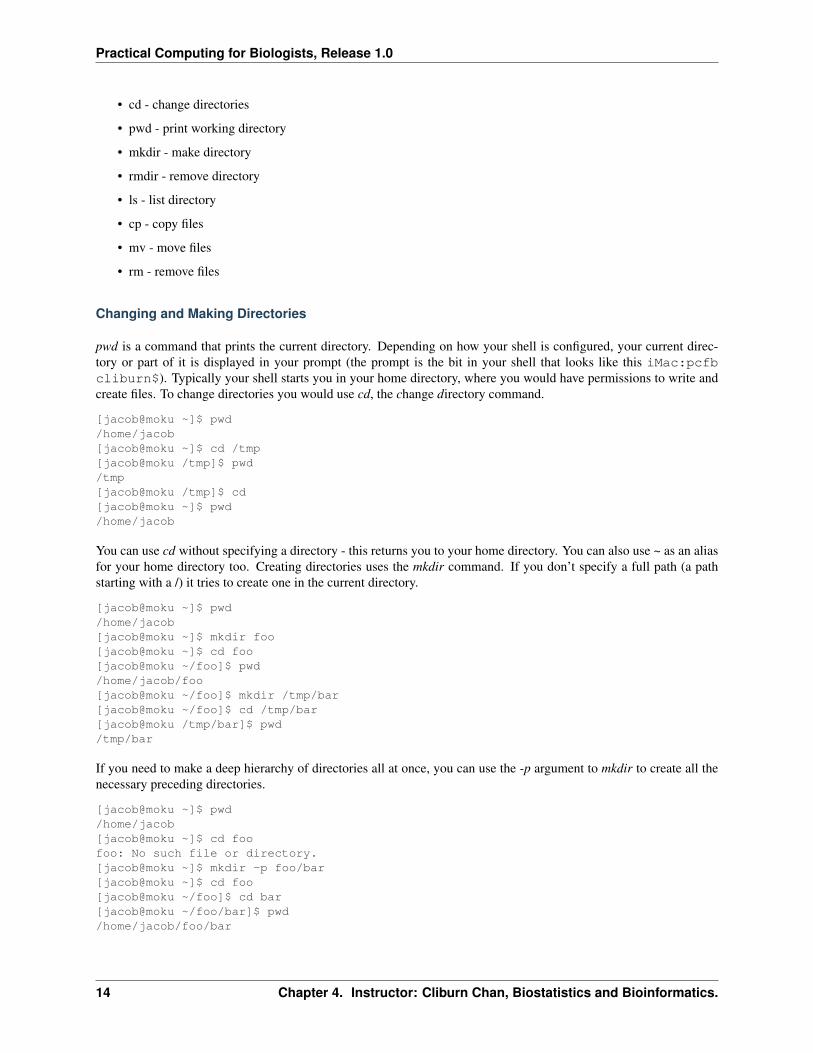
Changing and Making Directories
pwd is a command that prints the current directory. Depending on how your shell is configured, your current direc-tory or part of it is displayed in your prompt (the prompt is the bit in your shell that looks like this iMac:pcfbcliburn$). Typically your shell starts you in your home directory, where you would have permissions to write andcreate files. To change directories you would use cd, the change directory command.
[jacob@moku ~]$ pwd/home/jacob[jacob@moku ~]$ cd /tmp[jacob@moku /tmp]$ pwd/tmp[jacob@moku /tmp]$ cd[jacob@moku ~]$ pwd/home/jacob
You can use cd without specifying a directory - this returns you to your home directory. You can also use ~ as an aliasfor your home directory too. Creating directories uses the mkdir command. If you don’t specify a full path (a pathstarting with a /) it tries to create one in the current directory.
[jacob@moku ~]$ pwd/home/jacob[jacob@moku ~]$ mkdir foo[jacob@moku ~]$ cd foo[jacob@moku ~/foo]$ pwd/home/jacob/foo[jacob@moku ~/foo]$ mkdir /tmp/bar[jacob@moku ~/foo]$ cd /tmp/bar[jacob@moku /tmp/bar]$ pwd/tmp/bar
If you need to make a deep hierarchy of directories all at once, you can use the -p argument to mkdir to create all thenecessary preceding directories.
[jacob@moku ~]$ pwd/home/jacob[jacob@moku ~]$ cd foofoo: No such file or directory.[jacob@moku ~]$ mkdir -p foo/bar[jacob@moku ~]$ cd foo[jacob@moku ~/foo]$ cd bar[jacob@moku ~/foo/bar]$ pwd/home/jacob/foo/bar
14 Chapter 4. Instructor: Cliburn Chan, Biostatistics and Bioinformatics.

Practical Computing for Biologists, Release 1.0
The rmdir command removes directories. Directories must be empty to be removed. Just like mkdir, if a full pathis not specified it tries to remove the directory from the current directory. Similar to mkdir, the -p argument tries toremove all the preceding directories
[jacob@moku /tmp/bar]$ cd[jacob@moku ~]$ rmdir /tmp/bar[jacob@moku ~]$ rmdir -p foo/bar[jacob@moku ~]$ mkdir bar[jacob@moku ~]$ touch bar/foo[jacob@moku ~]$ rmdir barrmdir: bar: Directory not empty
touch is a command that creates an empty file. We will find out about it when we look at working with files
Examining directories
Now that we understand directories, we’d want to look at what files the directories contain. ls will list the files in adirectory.
[jacob@moku ~]$ lsA.txt B.txt C.txt bar[jacob@moku ~]$ ls barfoo
Just like mkdir, ls has several useful command line options. ls -l will list out all the extra properties of the directorylisted (file permissions, owner, last time modified). ls -a will list hidden files (those files whose name begin with a .).ls -F will append directories names / and (along with other symbols after other special file types).
[jacob@moku ~]$ ls -ltotal 5-rw-r--r-- 1 jacob jacob 32 May 25 08:48 A.txt-rw-r--r-- 1 jacob jacob 32 May 25 08:49 B.txt-rw-r--r-- 1 jacob jacob 64 May 25 08:53 C.txtdrwxr-xr-x 2 jacob jacob 3 May 23 15:54 bar[jacob@moku ~]$ ls -a. .cshrc .mail_aliases .rhosts A.txt bar.. .login .mailrc .shrc B.txt.bash_history .login_conf .profile .ssh C.txt[jacob@moku ~]$ ls -laFtotal 20drwxr-xr-x 4 jacob jacob 16 May 27 12:11 ./drwxr-xr-x 4 root wheel 5 May 23 15:12 ../-rw------- 1 jacob jacob 459 May 25 09:32 .bash_history-rw-r--r-- 1 jacob jacob 1014 May 23 15:12 .cshrc-rw-r--r-- 1 jacob jacob 257 May 23 15:12 .login-rw-r--r-- 1 jacob jacob 167 May 23 15:12 .login_conf-rw------- 1 jacob jacob 379 May 23 15:12 .mail_aliases-rw-r--r-- 1 jacob jacob 339 May 23 15:12 .mailrc-rw-r--r-- 1 jacob jacob 753 May 23 15:12 .profile-rw------- 1 jacob jacob 284 May 23 15:12 .rhosts-rw-r--r-- 1 jacob jacob 978 May 23 15:12 .shrcdrwx------ 2 jacob jacob 3 May 23 16:15 .ssh/-rw-r--r-- 1 jacob jacob 32 May 25 08:48 A.txt-rw-r--r-- 1 jacob jacob 32 May 25 08:49 B.txt-rw-r--r-- 1 jacob jacob 64 May 25 08:53 C.txtdrwxr-xr-x 2 jacob jacob 3 May 23 15:54 bar/
4.6. Basic Unix Commands 15

Practical Computing for Biologists, Release 1.0
Working with files
Coping files uses the cp command, copying from the first argument (source) to the last (destination):
[jacob@moku ~]$ cp A.txt bar/A.txt
if the destination is a directory it copes the file into the directory.
[jacob@moku ~]$ cp A.txt bar/[jacob@moku ~]$ ls barA.txt foo
You can also copy multiple files at once. cp will copy all the files listed on the command line into the directoryspecified in the last argument.
[jacob@moku ~]$ cp A.txt B.txt C.txt bar/[jacob@moku ~]$ ls barA.txt B.txt C.txt foo
Globbing will allow us to use many files at once rather than typing them all out explicitly. Globbing is a form ofwildcards.
Glob Effect* any number of any character? any single character[abc] one of a, b, or c
[jacob@moku ~]$ cp *.txt bar/[jacob@moku ~]$ ls barA.txt B.txt C.txt foo
or
[jacob@moku ~]$ cp ?.txt bar/[jacob@moku ~]$ ls barA.txt B.txt C.txt foo
or even
[jacob@moku ~]$ cp [ABC].txt bar/[jacob@moku ~]$ ls barA.txt B.txt C.txt foo
with the -r command line argument you can recursively copy whole directories
[jacob@moku ~]$ cp -r bar foo[jacob@moku ~]$ ls fooA.txt B.txt C.txt foo
Similar to the copy command is the move command mv.
[jacob@moku ~]$ mv A.txt foo[jacob@moku ~]$ mv [BC].txt foo[jacob@moku ~]$ mv foo/*.txt bar/[jacob@moku ~]$ mv foo baz
To remove files, use the rm command. A word of caution, there is no trash can or waste basket. Removed files aregone. It is very easy to accidentally shoot your self in the foot when blindly removing files.
[jacob@moku ~]$ rm bar/A.txt[jacob@moku ~]$ rm bar/[BC].txt
16 Chapter 4. Instructor: Cliburn Chan, Biostatistics and Bioinformatics.

Practical Computing for Biologists, Release 1.0
[jacob@moku ~]$ ls barfoo[jacob@moku ~]$ rm -rf bar/
the -r command line flag removes files recursively, while -f attempts to ignore permissions on the file. The combinationof -r and -f flags can be useful to remove whole directory tree. BE VERY CAREFUL using -r and -f flags.
4.6.2 Working with file contents
• cat - concatenate command
– pipes and redirects - Why concatenate prints to the screen
– globbing - Working with wildcards
• less - a more sensible way to look at the contents of file
• grep - searching for patterns in files
– basics of regular expressions
Examining files
The cat command will display files on the screen
[jacob@moku ~]$ cat A.txtThis is file A.It has 2 lines.[jacob@moku ~]$ cat B.txtThis is file B.It has3 lines.
cat will also concatenate files to print to the screen.
[jacob@moku ~]$ cat A.txt B.txtThis is file A.It has 2 lines.This is file B.It has3 lines.
Using redirects allows us to save the concatenated file.
[jacob@moku ~]$ cat A.txt B.txt > C.txt[jacob@moku ~]$ cat C.txtThis is file A.It has 2 lines.This is file B.It has3 lines.
> is a redirect to create a new file (and delete the old file if it exists). >> is the append redirect, while | (pipe) allowyou to send the output of one command as input to a new command.
[jacob@moku ~]$ cat [AB].txtThis is file A.It has 2 lines.This is file B.
4.6. Basic Unix Commands 17

Practical Computing for Biologists, Release 1.0
It has3 lines.
While cat is useful for displaying small files, longer files would page off the screen quickly. To display longer files, apage aware program will be used, less.
[jacob@moku ~]$ less <file name>
Common useful less keys
key effectG Go to the last line1G Go to the first line#G Go to line number #/foo Search forward for foo?foo Search Backward for fooq Quit less
Quitting (or how to escape when you are lost)
You may at some point find you self lost, and your prompt doing interesting things you don’t expect. Here are somekeys to try and get your prompt back in the state you expect.
• q
• Esc
• ctrl-d (sends an end of file saying there is no more input)
• typing Quit
• typing exit
• ctrl-c (sends a break, telling the program to abruptly halt)
Regexp, grep, and searching in files
The grep command allows you to tap into the powerful regular expression language to search the contests of file forcomplex patterns.
[jacob@moku ~]$ grep ’poor Yorick’ hamlet.txtHam. Let me see. [Takes the skull.] Alas, poor Yorick! I knew him,
The first argument passed to grep is the pattern to search for, in the above example poor Yorick.
Regular expressions provide the ability to search beyond known text, using wildcards to build complex patterns.
key Meaning. any single character+ one or more of the preceding character* zero or more of the preceding character^ matches the beginning of the line$ matches the end of the line[abc] matches a singular character of a, b, or c
so to find all the lines beginning with the word HAMLET and end withs DEMARK
18 Chapter 4. Instructor: Cliburn Chan, Biostatistics and Bioinformatics.

Practical Computing for Biologists, Release 1.0
[jacob@moku ~]$ grep ’^HAMLET.*DENMARK$’ hamlet.txtHAMLET, PRINCE OF DENMARK
Ever wonder how many lines in hamlet contain eight l’s in them?
[jacob@moku ~]$ grep ’l.*l.*l.*l.*l.*l.*l.*l’ hamlet.txtTill then sit still, my soul. Foul deeds will rise,all welcome. We’ll e’en to’t like French falconers, fly atmarried already- all but one- shall live; the rest shall keep as
Clown. I like thy wit well, in good faith. The gallows does well.
4.6.3 Man Pages
Unix documentation is typically stored in man pages acces by the man command. Try typing man cat into the consoleto see the manual page for the cat command. Note, man pages are notoriously terse, technical, and often confusing tonew users, so while learning it may be better to ask google instead, but if all you want is to know optional commandarguments the man page is the first place to look.
4.6.4 Exercise
Make a directory in your home folder named spam containing subfolders eggs, bacon, foo and bar and then removespam/foo and spam/bar
4.7 Using a text editor and regular expressions
4.7.1 What is a text editor?
Unlike a word processor, a text editor only handles plain text (i.e. no graphics or fancy formating). However, in return,text editors provide powerful tools for manipulating text, including the ability to use regular expressions, highlightdifferences between two or more files, and search and replace functionality on steroids. Since most data is available inor can be exported to plain text, and computer programs are written in plian text, a text editor is one of the most basicand useful applcations for anyone dealing with massive amounts of data. Text is universal - unlike binary formats (tryto open a WordPerfect 4.2 document), text documents are editable on any platform, and will still be readable in 30years time.
4.7.2 First look
This session will asume that you are using the TextWrangler editor on a Mac. The functionality of most text editors isvery similar, and you should be able to follow along if you are using a different editor. We will take the lazy optionof familiarizing you to TextWrangler by using the official tutorial. Open TextWrangler and take a few minutes tofamiliarize yourself with its anatomy - look at the menus, toolbars, icons etc. Most of this should be pretty familiarto you from other programs. Open the file Lorem ipsum.txt in the Tutorial Examples/Lesson 3 folder. Now read thedescription of the toolbar on Page 10 of the tutorial.
4.7.3 Mini-exercise
When you first open the Lorem ipsum.txt file, it looks like
4.7. Using a text editor and regular expressions 19

Practical Computing for Biologists, Release 1.0
Use the TextWrangler toolbar Text Options to get here
Then use the splitbar to split into two windows
Now drag the splitbar all the way to the top to get back a single window.
4.7.4 Finding and replacing
You can read all about TextWrangler in the tutorial at your leisure at home, but most things such as cut, copy and pasteand undo/redo work as expected. Since we have a lot to cover, we’ll just skip ahead to lesson 7. Open the file Findand Replace Sample.txt in the Lesson 7 folder and work through the exercise on page 39.
Next, open the Email Table.txt file in the Lesson 7 folder and work through the exercise on page 42 to learn how to dosearch and replace on invisible characters.
20 Chapter 4. Instructor: Cliburn Chan, Biostatistics and Bioinformatics.
Practical Computing for Biologists, Release 1.0
4.7.5 Regular expressions
We now come to the main part of this session, which is how to use regular expressions (or regex) for text manipulationdescribed in pages 44 to 51 of the TextWrangler tutorial. You have already come across regular expressions in theUnix session - now you will see how to use them to manipulate text files.
We’ll continue with the cats and dogs file just to get comfortable with the basic elements of regular expressions. Openthe Find dialog and check the Grep and Wrap around boxes. The Grep option tells TextWrangler that we areusing regular expressions, and wrap around that we want to do search and replace on the whole document regardlessof where our cursor/insertion point is. If at any point you get confused over the next few paragraphs, look at theexamples from page 47-49 for concrete illustrations of how to use regular expressions.
On page 45, there is a table of Wildcards. Put a period . in the Find box and click Next to see what matches. Keepclicking Next - you will see that the . matches every character as advertised. Next try \s in the Find box and clickNext. What does it match? Repeat for all the Wildcards to get a good intuition of what each wildcard matches.
Now do the same with the Class patterns. Feel free to edit the text to include new words or numbers if you are curiousas to how they will be matched. Also experiment with creating your own class search patterns - for example, whatwould a class to match DNA nucleotide symbols look like?
Now try the Repetition patterns *, *?, +, +? and ?. There is another repetition pattern {n, m} that means match atleast n but not more than m of the previous character or pattern. If n is left out, we have {,m} which means match nomore than m characters or patterns. If m is left out, we have {n,} which means match at least n occurrences. What isthe difference between * and *? or + and +?? When would you use the greedy and non-greedy versions?
Now figure out what the ^ and $ positional assertions and the alternation patterns mean. You can use parenthesis toenclose alternations if you need to also match stuff before and/or after the alternation.
4.7.6 Mini-exercise
1. Construct a regular expression to find two or more consecutive vowels in the cats and dogs file.
2. Use a regular expression pattern to delete all punctuation from the example.
3. Use a positional assertion with the alternation pattern to find all cat, cats, dog or dogs that occur at the end asentence. You should find that the ends of sentences 1, 3, 5, 9 and 11 match.
4.7.7 Subpatterns and replace patterns
Regular expressions really begin to show their power when we use subpatterns and replace patterns. This can be alittle tricky to wrap your head around when encountered for the first time, so we start with some simple contrivedexamples to give you some practice.
Subpatterns are simply any regular expression enclosed by parenthesis. For example, (.) is a subpattern that matchesany character, just like . by itself. However, we can refer to captured subpatterns to refer to whatever is in theparenthesis. For example, what does the regex (.)\1 find? See if you can guess, then use TextWrangler to check ifyou were correct.
We can also use the captured subpatterns in the replace pattern. Here again, \1 refers to the first regex in parenthesis,2‘ to the second one etc, and & to refer to the full regular expression matched (not just an individual subpattern). Asan example, what does putting (.)\1([aeiou]+) in the Find box and &\2\1& do? Test it out in TextWrangler tofind out what word is changed and what it is changed to.
4.7.8 Exercise
Open the file Ch3observations.txt in the examples folder. It looks like this
4.7. Using a text editor and regular expressions 21

Practical Computing for Biologists, Release 1.0
13 January, 1752 at 13:53 -1.414 5.781 Found in tide pools
17 March, 1961 at 03:46 14 3.6 Thirty specimens observed
1 Oct., 2002 at 18:22 36.51 -3.4221 Genome sequenced to confirm
20 July, 1863 at 12:02 1.74 133 Article in Harper’s
Write a regular expression to convert it into this:
1752 Jan. 13 13 53 -1.414 5.781
1961 Mar. 17 03 46 14 3.6
2002 Oct. 1 18 22 36.51 -3.4221
1863 Jul. 20 12 02 1.74 133
Hint: Construct a regular expression to match one single line. Look at the patterns that you must capture fromthe original to perform the conversion. Construct the appropriate subpatterns to do so. Now construct the regularpatterns between the subpatterns to match the unwanted separating characters. When you have a regular expressionthat matches a single line, check by clicking Next - the highlighted match should jump from one complete line to theother. Now use the references \1, \2 etc, re-ordering if necessary, and adding in filler such as extra punctuation ortabs to construct the desired replacement string. Save the regular expression by clicking the little g button on the Finddialog box and clicking Save .... Now hit Replace and see if it does what you expect. If it works, hit replace a fewmore times or click Replace All. If it doesn’t work, Undo and try again.
If you are totally lost and about to pull all your hair out, the construction of the solution is described in detail on pages38-40 of the PCfB textbook. However, you should not peek at the answer without trying for at least 15 minutes.
4.8 Remote computing and web page generation
Sometimes it is useful to be able to synchronize files or execute programs on a remote computer, or to transfer filesfrom one computer to another. This can be easily done from the command line very easily using the ssh, scp andrsync commands.
The ssh (secure shell) command allows you to securely connect to a remote computer for which you have access. Forexample, you can access your account on the Duke system:
eris:pcfb cliburn$ ssh [email protected]@login.oit.duke.edu’s password:Last login: Sat May 26 10:14:19 2012 from 152.3.189.147########################################################################### ## ***** ATTENTION ***** ATTENTION ***** ## ## This is a Duke University computer system. This computer system, ## including all related equipment, networks and network devices ## (includes internet access) are provided only for authorized Duke ## University use. Duke University computer systems may be monitored for ## all lawful purposes, including to ensure that their use is authorized, ## for management of the system, to facilitate protection against ## unauthorized access, and to verify security procedures, survivability, ## and operational security. During monitoring, information may be ## examined, recorded , copied , and used for authorized purposes. All ## information, including personal information, placed on or sent over ## this system may be monitored. use of this Duke University computer ## system, authorized or unauthorized, constitutes consent to ## monitoring. Unauthorized use of this Duke University computer system ## may subject you to criminal prosecution. Evidence of unauthorized use #
22 Chapter 4. Instructor: Cliburn Chan, Biostatistics and Bioinformatics.

Practical Computing for Biologists, Release 1.0
# collected during monitoring may be used for administrative, criminal, ## or other adverse action. Use of this system constitutes consent to ## monitoring for all lawful purposes. ###########################################################################
Self provisioned systems are now available for remote usage through OIT’s Virtual Computing Lab service. To reserve your own virtual machine please visit vcl.oit.duke.edu. Additional software images will be added to this service in the coming months.Mon May 28 00:44:43 EDT 2012[ccc14@login5 ~]$ lsAFSDocs public_html Sites[ccc14@login5 ~]$
If you know the IP address of a Linux or Mac computer that you have login rights to, you can usually connect to it viassh. For example, this is how we typically access departmental servers or computing workstations from home. If youwork with the Duke Beowulf cluster, you will also use ssh to connect and run your programs remotely.
If you can ssh to a computer, you can also copy files to or from the remote computer using scp (secure copy). Hereis an example:
[ccc14@login5 ~]$ cat > remote.txtThis is my remote file on lgoin.oit.duke.edu[ccc14@login5 ~]$ exitlogoutConnection to login.oit.duke.edu closed.eris:pcfb cliburn$ scp [email protected]:~/remote.txt [email protected]’s password:remote.txt 100% 45 0.0KB/s 00:00eris:pcfb cliburn$ cat remote.txtThis is my remote file on lgoin.oit.duke.edu
If you wish to synchronize entire directory trees between computers, it is more efficient to use rsync which performsdata compression, only tranfers files that are differnet, and allows resuming of interrupted transfers. For example,rsync is a simple way to back up your files to another computer.
eris:tmp cliburn$ rsync -avz foo [email protected]:~/[email protected]’s password:building file list ... donefoo/foo/foo.txtfoo/bar/foo/bar/bar.txtfoo/bar/baz/foo/bar/baz/baz.txt
sent 376 bytes received 104 bytes 73.85 bytes/sectotal size is 75 speedup is 0.16
The flags -avz are short for --archive, --verbose and --compress. The --archive flag preserves sym-bolic links and is perfect for remote backups. As usual, you can look at man rsync if you want to know the detailsof how rsync works.
4.8.1 Web page construction with sphinx
Sphinx (http://sphinx.pocoo.org/) is a Python tool to create documentation, but it is also great for creating highlystructured webpages with minimal effort. The entire workshop website was created with Sphinx.
We start by asking Sphinx to generate the initial directory for us with the sphinx-quickstart command. Theprogram will ask some configuration questions - you can just accept the defaults or give any sensible answer for now- the options can all be changed later if necessary.
4.8. Remote computing and web page generation 23

Practical Computing for Biologists, Release 1.0
eris:tmp cliburn$ sphinx-quickstart homepageWelcome to the Sphinx 1.1.2 quickstart utility.
Please enter values for the following settings (just press Enter toaccept a default value, if one is given in brackets).
Selected root path: homepage
You have two options for placing the build directory for Sphinx output.Either, you use a directory "_build" within the root path, or you separate"source" and "build" directories within the root path.> Separate source and build directories (y/N) [n]:
Inside the root directory, two more directories will be created; "_templates"for custom HTML templates and "_static" for custom stylesheets and other staticfiles. You can enter another prefix (such as ".") to replace the underscore.> Name prefix for templates and static dir [_]:
The project name will occur in several places in the built documentation.> Project name: Demo home page> Author name(s): Cliburn Chan
Sphinx has the notion of a "version" and a "release" for thesoftware. Each version can have multiple releases. For example, forPython the version is something like 2.5 or 3.0, while the release issomething like 2.5.1 or 3.0a1. If you don’t need this dual structure,just set both to the same value.> Project version: 0.0> Project release [0.0]:
The file name suffix for source files. Commonly, this is either ".txt"or ".rst". Only files with this suffix are considered documents.> Source file suffix [.rst]:
One document is special in that it is considered the top node of the"contents tree", that is, it is the root of the hierarchical structureof the documents. Normally, this is "index", but if your "index"document is a custom template, you can also set this to another filename.> Name of your master document (without suffix) [index]:
Sphinx can also add configuration for epub output:> Do you want to use the epub builder (y/N) [n]:
Please indicate if you want to use one of the following Sphinx extensions:> autodoc: automatically insert docstrings from modules (y/N) [n]:> doctest: automatically test code snippets in doctest blocks (y/N) [n]:> intersphinx: link between Sphinx documentation of different projects (y/N) [n]:> todo: write "todo" entries that can be shown or hidden on build (y/N) [n]:> coverage: checks for documentation coverage (y/N) [n]:> pngmath: include math, rendered as PNG images (y/N) [n]:> mathjax: include math, rendered in the browser by MathJax (y/N) [n]:> ifconfig: conditional inclusion of content based on config values (y/N) [n]:> viewcode: include links to the source code of documented Python objects (y/N) [n]:
A Makefile and a Windows command file can be generated for you so that youonly have to run e.g. ‘make html’ instead of invoking sphinx-builddirectly.> Create Makefile? (Y/n) [y]:
24 Chapter 4. Instructor: Cliburn Chan, Biostatistics and Bioinformatics.

Practical Computing for Biologists, Release 1.0
> Create Windows command file? (Y/n) [y]:
Creating file homepage/conf.py.Creating file homepage/index.rst.Creating file homepage/Makefile.Creating file homepage/make.bat.
Finished: An initial directory structure has been created.
You should now populate your master file homepage/index.rst and create other documentationsource files. Use the Makefile to build the docs, like so:
make builderwhere "builder" is one of the supported builders, e.g. html, latex or linkcheck.
The next thing to do is to cd homepage to enter the directory that was just created for us and edit the conf.pyfile to setup a configuraiton that we like. The only change to be made for now is to change the html_theme fromdefautl to agogo to match our workshop website theme. The themes that come with Sphinx can be viewed athttp://sphinx.pocoo.org/theming.html.
The first page to edit is the index.rst file. The rst extension is for ReStructuredText, a simple plain textmarkup language that is much easier to work with than HTML. Look at the primer on ReStructuredText athttp://sphinx.pocoo.org/rest.html to see examples of how to use it. Open the index.rst file in your text editor:
.. Demo home page documentation master file, created bysphinx-quickstart on Mon May 28 01:12:56 2012.You can adapt this file completely to your liking, but it should at leastcontain the root ‘toctree‘ directive.
Welcome to Demo home page’s documentation!==========================================
Contents:
.. toctree:::maxdepth: 2
Indices and tables==================
* :ref:‘genindex‘
* :ref:‘modindex‘
* :ref:‘search‘
Since this is to be a home page rather than documentation page, we can simplify the structure. Edit the file so that thelast part looks like this:
Contents:
.. toctree:::maxdepth: 2:hidden:
Home <self>researchpublications
We want to keep the table of contents hidden, and have set up a simple structure where the home page (index.html)
4.8. Remote computing and web page generation 25

Practical Computing for Biologists, Release 1.0
links to a research.html and a publications.html file. Just as the index.html file will be generated by thiis index.rst file,the other two files are also generated by a research.rst and publications.rst file that we write using ReStructuredText.The full contents of the 3 rst files are included verbatim for reference:
4.8.2 index.rst
Cliburn’s very boring home page==========================================
Stuff I do-------------------
Tongue ribeye pig, tenderloin turducken salami frankfurter stripsteak. T-bone turducken meatball flank, beef ribs brisket cornedbeef tail. Ball tip tongue flank beef ribs, biltong tri-tip salamichicken sausage leberkas chuck tail. Kielbasa shankle pork chopsirloin, leberkas bresaola tail. Ham hamburger venison sausagebiltong, pork loin brisket pig sirloin pastrami short loin shankchicken. Pig andouille leberkas beef short loin ribeye turkey hamhock. Cow ham kielbasa, capicola short ribs brisket shoulderpancetta t-bone pork belly tri-tip pork loin tenderloin.
Ground round pork belly pastrami pork chop, drumstick corned beeft-bone tail bresaola filet mignon meatloaf. Boudin spare ribs hamhock short loin. Prosciutto ham hock sausage, biltong leberkasturkey hamburger pork meatball bresaola pork belly. Shankle tri-tipfrankfurter ribeye leberkas ham hock, tongue beef ribs speck venisonpork chop andouille chuck. Rump pastrami bresaola, strip steak shortloin andouille pork chop beef boudin capicola bacon shank prosciuttobeef ribs swine. Meatloaf leberkas pancetta beef.
More stuff I do--------------------
Enim do boudin officia labore tail. Pork exercitation short ribsdeserunt laboris, tenderloin drumstick in dolor tongue sunt ex. Hamhock t-bone exercitation pork loin non mollit. Jowl boudin magnaadipisicing in dolore. Brisket quis shoulder nostrud temporea. Aliquip officia consequat deserunt, dolore nostrud est tri-tiput pancetta speck shank excepteur. Sausage cillum ground round velitrump, dolore laboris.
Commodo consectetur ut, officia proident eu cillum jowl aute flanksausage ut beef ribs. Deserunt occaecat pariatur elit. Pork chop uttempor, enim aliqua laborum cillum eiusmod t-bone occaecat autelaboris labore. Ham hock turkey beef nostrud excepteurdolor. Consectetur meatball chicken deserunt exercitation, cornedbeef beef in short ribs ut ea velit beef ribs. Enim andouille in,dolore ut meatball ea ut tail proident short ribs leberkas groundround filet mignon.
Andouille sirloin chicken tempor aute, cow salami commodo doloreleberkas culpa in ea esse. Id ground round tongue velit. Ex elitminim sirloin fatback laboris. Irure andouille shankle cupidatat,nostrud bresaola id shank do jowl. Swine sirloin pork loin,prosciutto bresaola rump cillum in exercitation capicola.
26 Chapter 4. Instructor: Cliburn Chan, Biostatistics and Bioinformatics.

Practical Computing for Biologists, Release 1.0
Contents:
.. toctree:::maxdepth: 2:hidden:
Home <self>researchpublications
4.8.3 research.rst
Cliburn’s boring research page=================================================
Current research interests---------------------------------------
1. Bacon2. Pork rind3. Trotters
.. image:: bacon.jpg:width: 60%
Past research interests----------------------------------------
1. LOL cats
.. image:: Lolcat.JPG
4.8.4 publications.rst
Not really Cliburn’s publications================================
First 5 hits on Pubmed search for "Sphinx"---------------------------------------------
1. Quadrature RF Coil for In Vivo Brain MRI of a Macaque Monkey ina Stereotaxic Head Frame. Roopnariane CA, Ryu YC, Tofighi MR,Miller PA, Oh S, Wang J, Park BS, Ansel L, Lieu CA, Subramanian T,Yang QX, Collins CM. Concepts Magn Reson Part B Magn ResonEng. 2012 Feb;41B(1):22-27. Epub 2012 Feb 18. PMID: 22611340[PubMed]
2. The place of general practitioners in cancer care inChampagne-Ardenne. Tardieu E, Thiry-Bour C, Devaux C, Ciocan D,de Carvalho V, Grand M, Rousselot-Marche E, Jovenin N. BullCancer. 2012 May 1;99(5):557-562. PMID: 22522646 [PubMed - assupplied by publisher]
4.8. Remote computing and web page generation 27
Practical Computing for Biologists, Release 1.0
3. Spontaneous Endometriosis in a Mandrill (Mandrillus sphinx).Nakamura S, Ochiai K, Ochi A, Ito M, Kamiya T, Yamamoto H. J CompPathol. 2012 Apr 18. [Epub ahead of print] PMID: 22520805[PubMed - as supplied by publisher]
4. [Reality of healthcare access for migrant children in Mayotte].Baillot J, Luminet B, Drouot N, Corty JF. Bull Soc PatholExot. 2012 May;105(2):123-9. Epub 2012 Mar 1. French. PMID:22383116 [PubMed - in process]
5. Craniodental features in male Mandrillus may signal size andfitness: an allometric approach. Klopp EB. Am J PhysAnthropol. 2012 Apr;147(4):593-603. doi: 10.1002/ajpa.22017. Epub2012 Feb 10. PMID: 22328467 [PubMed - indexed for MEDLINE]
4.8.5 HTML Generation
With these files written, we now ask Sphinx to generate the HTML
eris:homepage cliburn$ make htmlsphinx-build -b html -d _build/doctrees . _build/htmlMaking output directory...Running Sphinx v1.1.2loading pickled environment... not yet createdbuilding [html]: targets for 3 source files that are out of dateupdating environment: 3 added, 0 changed, 0 removedreading sources... [100%] research
Not really Cliburn’s publications================================looking for now-outdated files... none foundpickling environment... donechecking consistency... donepreparing documents... donewriting output... [100%] researchwriting additional files... genindex searchcopying images... [100%] bacon.jpgcopying static files... donedumping search index... donedumping object inventory... donebuild succeeded, 1 warning.
Build finished. The HTML pages are in _build/html.
And now the directory looks like this:
eris:homepage cliburn$ lsLolcat.JPG _templates make.batMakefile bacon.jpg publications.rst_build conf.py research.rst_static index.rst
4.8.6 Copy generated HTML to public_html on Duke server
Now all we need to do is to rsync the _build/html folder to the Duke server:
28 Chapter 4. Instructor: Cliburn Chan, Biostatistics and Bioinformatics.
Practical Computing for Biologists, Release 1.0
eris:homepage cliburn$ rsync -avz _build/html/ [email protected]:~/public_html/[email protected]’s password:building file list ... donecreated directory /afs/acpub/users/c/c/ccc14/public_html/homepage./.buildinfogenindex.htmlindex.htmlobjects.invpublications.htmlresearch.htmlsearch.htmlsearchindex.js_images/_images/Lolcat.JPG_images/bacon.jpg_sources/_sources/index.txt_sources/publications.txt_sources/research.txt_static/_static/agogo.css_static/ajax-loader.gif_static/basic.css_static/bgfooter.png_static/bgtop.png_static/comment-bright.png_static/comment-close.png_static/comment.png_static/doctools.js_static/down-pressed.png_static/down.png_static/file.png_static/jquery.js_static/minus.png_static/plus.png_static/pygments.css_static/searchtools.js_static/underscore.js_static/up-pressed.png_static/up.png_static/websupport.js
sent 164472 bytes received 792 bytes 22035.20 bytes/sectotal size is 286369 speedup is 1.73
Now, if we navigate to http://www.duke.edu/~ccc14/homepage/, we will see the homepage and the links on the sidebarto publications and research work as well.
4.8. Remote computing and web page generation 29

Practical Computing for Biologists, Release 1.0
4.9 Python Basics I
4.9.1 Why program?
Biology is increasingly data-rich. And the amount of data is growing exponentially, as I am sure you are all only toowell aware. Wouldn’t it be really nice if you had some unpaid slaves that would help you sort through your data, checkfor problems, find the most interesting bits, and generate pretty pictures for you to include in your next manuscript?Well, you are in luck, for the computer is a slave factory, and the slaves are called programs. And today, I have someslaves to give away ...
4.9.2 What can my slave do?
In this workshop, we will focus on 3 types of jobs for our slaves that are essential whenever there is a lot of data:
1. Data munging
2. Data analysis
3. Data visualization
Data munging means taking that error-riddled, color-coded, highly redundant Excel spreadsheet that biologists loveto create, and cleaning, parsing and proofing it so that it is suitable for analysis. There is a related skill of how to
30 Chapter 4. Instructor: Cliburn Chan, Biostatistics and Bioinformatics.

Practical Computing for Biologists, Release 1.0
create persistent data stores that allow you to slice and dice well-structured data that will be briefly touched uponin the session on :doc:Data management and relational databasesI</database>, but will requireanother full workshop to cover in any depth.
Data analysis is largely about how to do statistics. We will show very simple examples of analysis in :doc:Dataanalysis with Python</analysis>, but the proper cultivation of the statistical way of thinking probablyrequires not just another workshop, but returning to graduate school.
Finally, there are two main reasons for data visualization - the first is for exploratory data analysis, since the humanbrain is highly optimized to detect patterns in pictures; and the second is for communicating results, since everybiologist I’ve ever met is only ever interested in the figures in a paper and never the raw data. Making pictures fromdata for exploratory analysis and communication are covered in NumPy and Matplotlib</numerics> andthe creation of schematics to illustrate concepts in :doc:Vector graphics with Inkscape</inkscape>.
But first - in order to tell your slave how to do these jobs, you need to think like a programmer.
4.9.3 Thinking like a programmer
Computers are stupid. And very literal. So to be able to program, we need to tell the computer what to do in verysimple language without any ambiguity. Almost all programs we will deal with involve only 5 basic operations:
1. Get input data2. Store data in variables3. Do some calculation or check logic4. Repeat5. Generate some output
For now, we simply define a variable as a name we give to data so that we can retrieve it later. The other terms shouldbe familiar to everyone.
For example, here is a simple example that checks if a word is a palindrome:
1 # get input and store in variable word2 word = raw_input("Enter a word: ")3 # check if word is the same when reversed4 if word == word[::-1]:5 print "%s is a palindrome!" % word6 else:7 print "%s is a regular old word" % word
Here is another program that makes use of these 5 concepts:
1 """Count the number of vowels in a name."""2
3 # input data and store in variable name4 name = raw_input("What’s your name? ")5 # store count of vowels in variable num_vowels6 num_vowels = 07 # repeat updating of vowel count8 for vowel in ’aeiou’:9 # simple calculation (count occurences of vowel in string)
10 num_vowels += name.count(vowel)11 # output result12 print "Hello %s, there are %d vowels in your name." % (name, num_vowels)
Since the 5 operations are about all that a computer can do, even big complex projects must boil down to smaller tasksthat mix and match these operations. Essentially, if you know these 5 operations, you know how to program. The restare details.
4.9. Python Basics I 31

Practical Computing for Biologists, Release 1.0
4.9.4 Introducing Python
We will learn to program in a language called Python, named after the British comedy skit Monty Python. Pythonis possibly the simplest programming language to learn and has an amazing range of libraries for just about anybiomedical data processing need, making it an ideal first language for biologists to learn. When you are comfortablewith Python, a very useful second language to learn is R, another open source language specialized for statisticalanalysis.
Python is an interpreted language, meaning that instructions are executed as soon as you complete a programmingstatement. To see the Python interpreter in action, we will use the IPython interpreter, which you can start by openinga Terminal window and typing ipython, after which you will see this welcome message:
eris:pcfb cliburn$ ipythonEnthought Python Distribution -- http://www.enthought.com
Python 2.6.6 |EPD 6.3-2 (32-bit)| (r266:84292, Sep 23 2010, 11:52:53)Type "copyright", "credits" or "license" for more information.
IPython 0.10.1 -- An enhanced Interactive Python.? -> Introduction and overview of IPython’s features.%quickref -> Quick reference.help -> Python’s own help system.object? -> Details about ’object’. ?object also works, ?? prints more.
There is also a vanilla python interpreter, but ipython provides so many nice features such as Unix shell integra-tion, tab completion, history etc that I hardly ever use the python interpreter. Try typing ? in ipython to see whatit offers. To exit the information screen, type q to quit. There are several ways to get more information about a Pythonlanguage feature - for example, what does the python range function do? Type help(range) or help rangeor range? or ?range.
4.9.5 Python as a calculator
To get comfortable with ipython, let’s just use it as a calculator:
In [1]: 1+2*3**2Out[1]: 19
In [2]: 3/2Out[2]: 1
In [3]: 3/2.0Out[3]: 1.5
In [4]: 13 % 4Out[4]: 1
In [5]: import math
In [6]: math.piOut[6]: 3.141592653589793
In [7]: math.eOut[7]: 2.718281828459045
In [8]: math.pi/4Out[8]: 0.7853981633974483
32 Chapter 4. Instructor: Cliburn Chan, Biostatistics and Bioinformatics.

Practical Computing for Biologists, Release 1.0
In [9]: math.sin(math.pi/4)Out[9]: 0.7071067811865475
In [10]: math.asin(math.sin(math.pi/4))Out[10]: 0.7853981633974482
In [11]: math.sqrt(16)Out[11]: 4.0
In [12]: 16**0.5Out[12]: 4.0
Note the gotcha in the [2] calculation - when both numerator and denominator are integers, the division operatorreturns an integer, which might not be what you want. Make either numerator or denominator a float (a number witha decimal point) as in [3] to get the usual answer.
4.9.6 Types
As we have already seen in the previous example, there is a difference between 2 and 2.0. In particular, they differ intype - 2 is an integer, while 2.0 is a float. Types are necessary so that Python can distinguish between different kindsof things that may have different behaviors. Here are the most commonly used basic types in Python:
1. Integers are natural numbers, ..., -3, -2, -1, 0, 1, 2, 3 ...
2. Floats are “decimal” numbers e.g. 0.01, 1e-6, math.pi etc
3. Bools are the values True and False
4. Strings are anything within single quotes, double quotes, or “triple” quotes such as ’hello’, "hello",”’hello”’ and """hello""".
While the first 3 types are atomic, strings are actually sequences of characters, and we can retrieve characters at specificpostions by indexing and slicing. An example of how we can slice and dice sequences is useful here:
In [1]: s = "My first string"
In [2]: s[0]Out[2]: ’M’
In [3]: s[1]Out[3]: ’y’
In [4]: s[-1]Out[4]: ’g’
In [5]: s[0:2]Out[5]: ’My’
In [6]: s[3:8]Out[6]: ’first’
In [7]: s[3:8:2]Out[7]: ’frt’
In [8]: s[::-1]Out[8]: ’gnirts tsrif yM’
Note that in Python, we count from zero, not one. Note also that a negative index means count backwards from theend of the sequence.
4.9. Python Basics I 33
Practical Computing for Biologists, Release 1.0
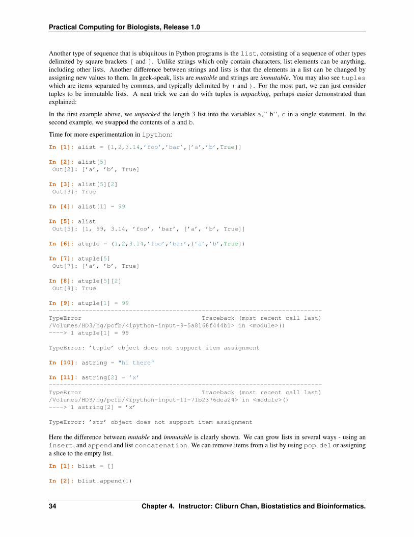
Another type of sequence that is ubiquitous in Python programs is the list, consisting of a sequence of other typesdelimited by square brackets [ and ]. Unlike strings which only contain characters, list elements can be anything,including other lists. Another difference between strings and lists is that the elements in a list can be changed byassigning new values to them. In geek-speak, lists are mutable and strings are immutable. You may also see tupleswhich are items separated by commas, and typically delimited by ( and ). For the most part, we can just considertuples to be immutable lists. A neat trick we can do with tuples is unpacking, perhaps easier demonstrated thanexplained:
In the first example above, we unpacked the length 3 list into the variables a,‘‘ b‘‘, c in a single statement. In thesecond example, we swapped the contents of a and b.
Time for more experimentation in ipython:
In [1]: alist = [1,2,3.14,’foo’,’bar’,[’a’,’b’,True]]
In [2]: alist[5]Out[2]: [’a’, ’b’, True]
In [3]: alist[5][2]Out[3]: True
In [4]: alist[1] = 99
In [5]: alistOut[5]: [1, 99, 3.14, ’foo’, ’bar’, [’a’, ’b’, True]]
In [6]: atuple = (1,2,3.14,’foo’,’bar’,[’a’,’b’,True])
In [7]: atuple[5]Out[7]: [’a’, ’b’, True]
In [8]: atuple[5][2]Out[8]: True
In [9]: atuple[1] = 99---------------------------------------------------------------------------TypeError Traceback (most recent call last)/Volumes/HD3/hg/pcfb/<ipython-input-9-5a8168f444b1> in <module>()----> 1 atuple[1] = 99
TypeError: ’tuple’ object does not support item assignment
In [10]: astring = "hi there"
In [11]: astring[2] = ’x’---------------------------------------------------------------------------TypeError Traceback (most recent call last)/Volumes/HD3/hg/pcfb/<ipython-input-11-71b2376dea24> in <module>()----> 1 astring[2] = ’x’
TypeError: ’str’ object does not support item assignment
Here the difference between mutable and immutable is clearly shown. We can grow lists in several ways - using aninsert, and append and list concatenation. We can remove items from a list by using pop, del or assigninga slice to the empty list.
In [1]: blist = []
In [2]: blist.append(1)
34 Chapter 4. Instructor: Cliburn Chan, Biostatistics and Bioinformatics.

Practical Computing for Biologists, Release 1.0
In [3]: blist.append(99)
In [4]: blist = blist + [3,4,5]
In [5]: blistOut[5]: [1, 99, 3, 4, 5]
In [6]: blist[2:2] = [’a’,’b’,’c’]
In [7]: blistOut[7]: [1, 99, ’a’, ’b’, ’c’, 3, 4, 5]
In [8]: blist[2:4] = []
In [9]: blistOut[9]: [1, 99, ’c’, 3, 4, 5]
In [10]: blist.pop()Out[10]: 5
In [11]: blistOut[11]: [1, 99, ’c’, 3, 4]
In [12]: del blist[3]
In [13]: blistOut[13]: [1, 99, ’c’, 4]
The final basic type we will look at is the dictionary. A dictionary consists of (key, value) pairs, wherethe key is an immutable type (e.g. a number, a string, a tuple) and the value is anything. We retrieve the value in adictionary by using the associated key. Dictionaries are delimited by { and }. For example, we can make a dictionaryof email addresses:
In [1]: emails = {}
In [2]: emails[’cliburn’] = ’[email protected]’
In [3]: emails[’jacob’] = ’[email protected]’
In [4]: emails[’cliburn’]Out[4]: ’[email protected]’
In [5]: emails.keys()Out[5]: [’jacob’, ’cliburn’]
In [6]: emails.values()Out[6]: [’[email protected]’, ’[email protected]’]
In [7]: emailsOut[7]: {’cliburn’: ’[email protected]’, ’jacob’: ’[email protected]’}
We can also think of dictionaries as fancy lists that are not restricted to consecutive integers for indexing. Note thatwe create dictionaries with curly braces {} but assign element to and retrieve elements from dictionaries with squarebrackets [key]. If the key is not found in the dictionary, Python will raise a KeyError exception and abort. To avoidthat, we can either check for the key before retrieval, tell Python to ignore KeyErrors in a try-except statement,or return a default value using the get method instead of [] to access the dictionary. Here are more examples ofdictionary creation and usage:
4.9. Python Basics I 35

Practical Computing for Biologists, Release 1.0
In [1]: zip([’a’,’b’,’c’,’d’], [1,2,3,4])Out[1]: [(’a’, 1), (’b’, 2), (’c’, 3), (’d’, 4)]
In [2]: adict = dict(zip([’a’,’b’,’c’,’d’], [1,2,3,4]))
In [3]: adictOut[3]: {’a’: 1, ’b’: 2, ’c’: 3, ’d’: 4}
In [4]: adict[’b’]Out[4]: 2
In [5]: adict.get(’e’, 0)Out[5]: 0
In [6]: adictOut[6]: {’a’: 1, ’b’: 2, ’c’: 3, ’d’: 4}
In [7]: adict.setdefault(’e’, 0)Out[7]: 0
In [8]: adictOut[8]: {’a’: 1, ’b’: 2, ’c’: 3, ’d’: 4, ’e’: 0}
Dictionaries can also be constructed from a list of (key, value) pairs (or 2-tuples). The zip function takes the firstelement from list 1 and the first element from list 2 to make a tuple, then does the same for the second element etc untilone or both lists are exhausted. It is used here to construct a list of pair from two matching lists of keys and values.The get method returns the default (second) argument when the key given by its first argument is not found in thedictionary. The setdefault method does the same thing, but additionally inserts the new key / default value intothe dictionary if not found. If we want to ingore missing keys but just retrieve values for valid keys, we can wrap thedictionary access in a try-except statement:
In [1]: adictOut[1]: {’a’: 1, ’b’: 2, ’c’: 3, ’d’: 4, ’e’: 0}
In [2]: for ch in "ajfljldjajfeljad":...: try:...: print adict[ch]...: except KeyError:...: pass...:...:
141014
The pass keyword means “do nothing”. Without the try-except statement, the program would crash with aKeyError‘ the first time ‘‘ch was not found in the dictionary keys a, b, c, d, e.
You might have noticed that we sometimes used a funny notation with a dot . between names, for examplelist.append(1). This is because Python is an object-oriented language, and these basic types are also classes.We won’t discuss classes here except to note that we use the dot notation to access values (attributes) and functions(methods) associated with the class. In ipython, hit the tab key after the dot to see what types are available.
In [1]: blistOut[1]: [1, 99, ’c’, 4]
36 Chapter 4. Instructor: Cliburn Chan, Biostatistics and Bioinformatics.

Practical Computing for Biologists, Release 1.0
In [2]: [b for b in dir(blist) if not b.startswith(’_’)]Out[2]:
[’append’,’count’,’extend’,’index’,’insert’,’pop’,’remove’,’reverse’,’sort’]
The code ‘‘ [b for b in dir(blist) if not b.startswith(‘_’)] ‘‘ is a list comprehension to show all the normalmethods of the list class, filtering out methods that look like __xxx__. The methods with __ prefixes and suffixesare “special” internal methods that we won’t use in this workshop. You can use help to find out what extend, indexetc do. The count, reverse and sort methods are quite simple:
In [1]: numlist = [3,1,4,1,5,1,6,9]
In [2]: numlist.sort()
In [3]: numlistOut[3]: [1, 1, 1, 3, 4, 5, 6, 9]
In [4]: numlist.reverse()
In [5]: numlistOut[5]: [9, 6, 5, 4, 3, 1, 1, 1]
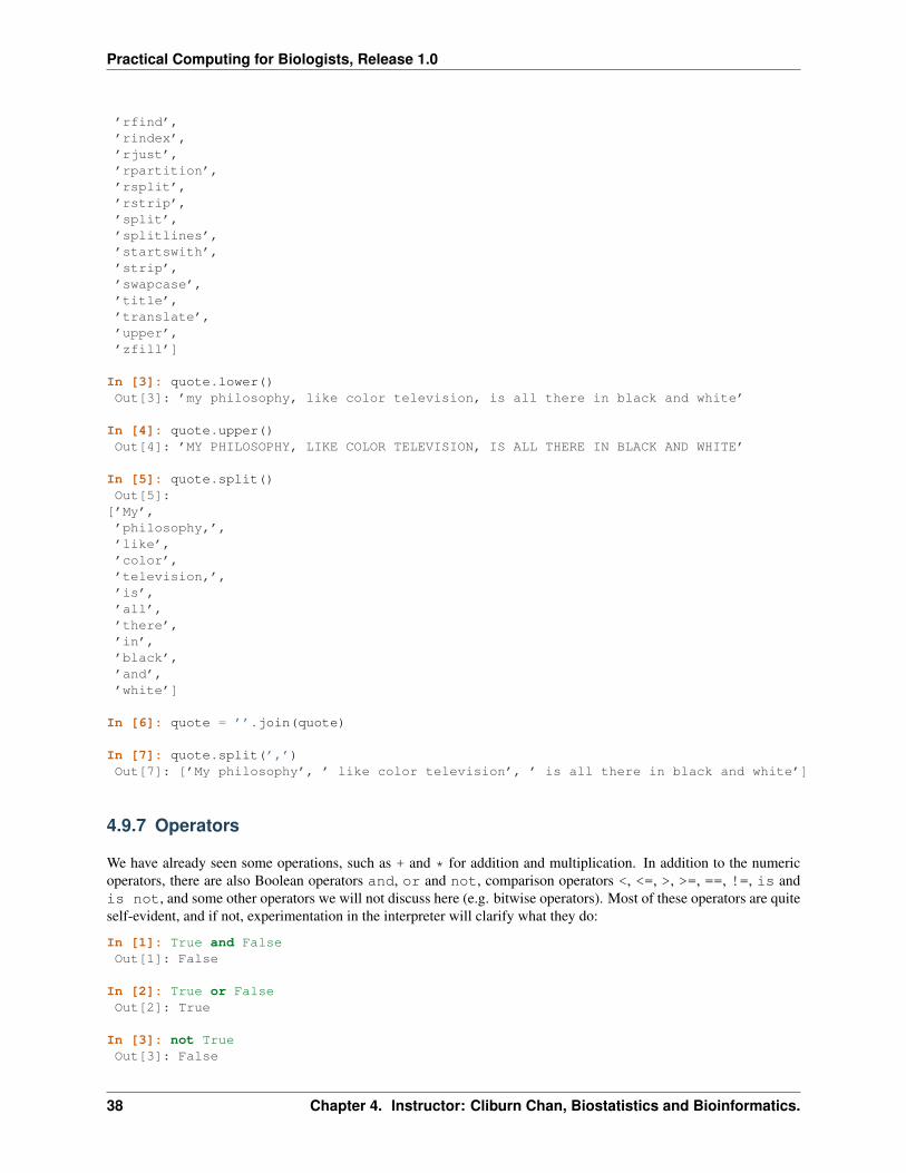
Strings have an even longer list of methods:
In [1]: quote = "My philosophy, like color television, is all there in black and white"
In [2]: [m for m in dir(quote) if not m.startswith(’_’)]Out[2]:
[’capitalize’,’center’,’count’,’decode’,’encode’,’endswith’,’expandtabs’,’find’,’format’,’index’,’isalnum’,’isalpha’,’isdigit’,’islower’,’isspace’,’istitle’,’isupper’,’join’,’ljust’,’lower’,’lstrip’,’partition’,’replace’,
4.9. Python Basics I 37
Practical Computing for Biologists, Release 1.0
’rfind’,’rindex’,’rjust’,’rpartition’,’rsplit’,’rstrip’,’split’,’splitlines’,’startswith’,’strip’,’swapcase’,’title’,’translate’,’upper’,’zfill’]
In [3]: quote.lower()Out[3]: ’my philosophy, like color television, is all there in black and white’
In [4]: quote.upper()Out[4]: ’MY PHILOSOPHY, LIKE COLOR TELEVISION, IS ALL THERE IN BLACK AND WHITE’
In [5]: quote.split()Out[5]:
[’My’,’philosophy,’,’like’,’color’,’television,’,’is’,’all’,’there’,’in’,’black’,’and’,’white’]
In [6]: quote = ’’.join(quote)
In [7]: quote.split(’,’)Out[7]: [’My philosophy’, ’ like color television’, ’ is all there in black and white’]
4.9.7 Operators
We have already seen some operations, such as + and * for addition and multiplication. In addition to the numericoperators, there are also Boolean operators and, or and not, comparison operators <, <=, >, >=, ==, !=, is andis not, and some other operators we will not discuss here (e.g. bitwise operators). Most of these operators are quiteself-evident, and if not, experimentation in the interpreter will clarify what they do:
In [1]: True and FalseOut[1]: False
In [2]: True or FalseOut[2]: True
In [3]: not TrueOut[3]: False
38 Chapter 4. Instructor: Cliburn Chan, Biostatistics and Bioinformatics.

Practical Computing for Biologists, Release 1.0
In [4]: 3 == 3Out[4]: True
In [5]: 3 == 4Out[5]: False
In [6]: 3 != 4Out[6]: True
In [7]: 3 > 4Out[7]: False
In [8]: 4 > 3Out[8]: True
In [9]: None is NoneOut[9]: True
In [10]: 0 is NoneOut[10]: False
In [11]: 0 is not NoneOut[11]: True
4.9.8 Control flow and loops
We now begin to get to the heart of programming - asking the computer to do mind-numbingly boring work many,many times. The way to perform repetitions is by looping, but before we go there, we will first learn about howto control the program flow with the if-else family of statements. Luckily, the if-else statement family doesexactly what you’d expect it to do:
In [1]: if ’math’ > ’football’:...: print ’Nerds rule’...: else:...: print ’Jocks rule’...:
Nerds rule
The structure of the if-else statement has the form:
if (condition is true):do A
else:do B
Here are some more examples of the if-else family:
In [1]: grade = None
In [2]: score = 86
In [3]: if (score > 93):...: grade = ’A’...: elif (score > 85):...: grade = ’B’...: elif (score > 70):...: grade = ’C’
4.9. Python Basics I 39

Practical Computing for Biologists, Release 1.0
...: else:
...: grade = ’D’
...:
In [4]: gradeOut[4]: ’B’
As you can see, the if statement can be used by itself without an else part with the understanding that if the conditionis not true, then nothing is done. If you need to make decisions based on many conditions, the if-[elif]-elseform is useful, where the final optional else statement will be executed if none of the others above it are true. Notethat the last example depends on the ordering of the conditions, and works because the if-elif-else statementworks from top to bottom. See if you can figure out why the code below doesn’t work as intended:
In [1]: score = 86
In [2]: grade = None
In [3]: if (score > 70):...: grade = ’C’...: elif (score > 85):...: grade = ’B’...: elif (score > 93):...: grade = ’A’...:
In [4]: gradeOut[4]: ’C’
OK, back to looping. There are two main ways to loop in Python using the for and while statements. The forstatement goes through a sequence of items one at a time, typically performing some work on that item as it iteratesover it. The examples below should make clear what a for loop does:
In [1]: range(10, 15)Out[1]: [10, 11, 12, 13, 14]
In [2]: for number in range(10, 15):...: print number...:
1011121314
In [3]: for char in ’abcde’:...: print char...:
abcde
In [4]: for name in [’adam’, ’eve’]:...: print name...:
adameve
40 Chapter 4. Instructor: Cliburn Chan, Biostatistics and Bioinformatics.

Practical Computing for Biologists, Release 1.0
Remember that strings, lists, tuples and dictionaries are all sequences, and hence iterable. So we can use the for loopon any of these. It is getting rather tedious to use the word sequence, so from now on, I will use lists, or strings ordictionaries, but you should remember that the looping constructs work on all of them. Another Python idiom that issometimes useful in looping is the use of enumerate to keep track of position (or index) while looping over a list.Here is how it is used:
In [1]: for i, name in enumerate([’cliburn’, ’jacob’, ’adam’]):...: print i, name...:
0 cliburn1 jacob2 adam
A common use of the for loop is to create a new list from an old one. For example, here is how you can create a list ofall the squares from 10 to 15.
In [1]: squares = []
In [2]: for i in range(10, 16):...: squares.append(i**2)...:
In [3]: squaresOut[3]: [100, 121, 144, 169, 196, 225]
Notice that to get the numbers [10,11,12,13,14,15], we call range(10, 16) since Python indexing in-cludes the start but excludes the end.
We can now combine if checks with loops to filter lists that we are constructing, only adding items to our list if theymeet certain conditions. Suppose we wanted to only collect the squares of the odd numbers and discard the even onein the previous example:
In [1]: oddsquares = []
In [2]: for i in range(10, 16):...: if i%2==1:...: oddsquares.append(i**2)...:
In [3]: oddsquaresOut[3]: [121, 169, 225]
This process of looping over a sequence and collecting the items in a list, filtering by some condition if necessary, is socommon that Python has a short cut way of doing it known as list comprehension. Here is the nicer list comprehensionversion of the above two examples:
In [1]: squares = [i**2 for i in range(10, 16)]
In [2]: squaresOut[2]: [100, 121, 144, 169, 196, 225]
In [3]: oddsquares = [i**2 for i in range(10, 16) if i%2==1]
In [4]: oddsquaresOut[4]: [121, 169, 225]
We can nest loops within each other - for example, to generate labels for a 96-well plate, we can do this list compre-hension:
4.9. Python Basics I 41

Practical Computing for Biologists, Release 1.0
In [1]: wells = [’%s%02d’ % (r, c) for r in ’ABCDEF’ for c in range(1, 13)]
In [2]: wells[:15]Out[2]:
[’A01’,’A02’,’A03’,’A04’,’A05’,’A06’,’A07’,’A08’,’A09’,’A10’,’A11’,’A12’,’B01’,’B02’,’B03’]
It might be clearer to understand what is happening using the longer version of creating an empty list, then usingnested for loops:
In [1]: wells = []
In [2]: for r in ’ABCDEF’:...: for c in range(1,13):...: wells.append(’%s%02d’ % (r, c))...:
In [3]: wells[:15]Out[3]:
[’A01’,’A02’,’A03’,’A04’,’A05’,’A06’,’A07’,’A08’,’A09’,’A10’,’A11’,’A12’,’B01’,’B02’,’B03’]
Don’t worry about the funny ‘%02d’ and ‘%s’ bits in the code. We will explain string interpolation in the nextsession. Congratulations! You have learnt the basic building blocks of a python program. Once you complete theexercise below, we will finish off our Python crash course with I/O and creating your own functions.
4.9.9 Storing and re-using programs
Using ipython is great for learning because of the instant feedback, but at some point you will want to save yourcode to use for another day. To do so, we use our text editor to write code in a file that ends with the extension ‘.py’.Open up a new page in TextWrangler, enter the following code:
42 Chapter 4. Instructor: Cliburn Chan, Biostatistics and Bioinformatics.
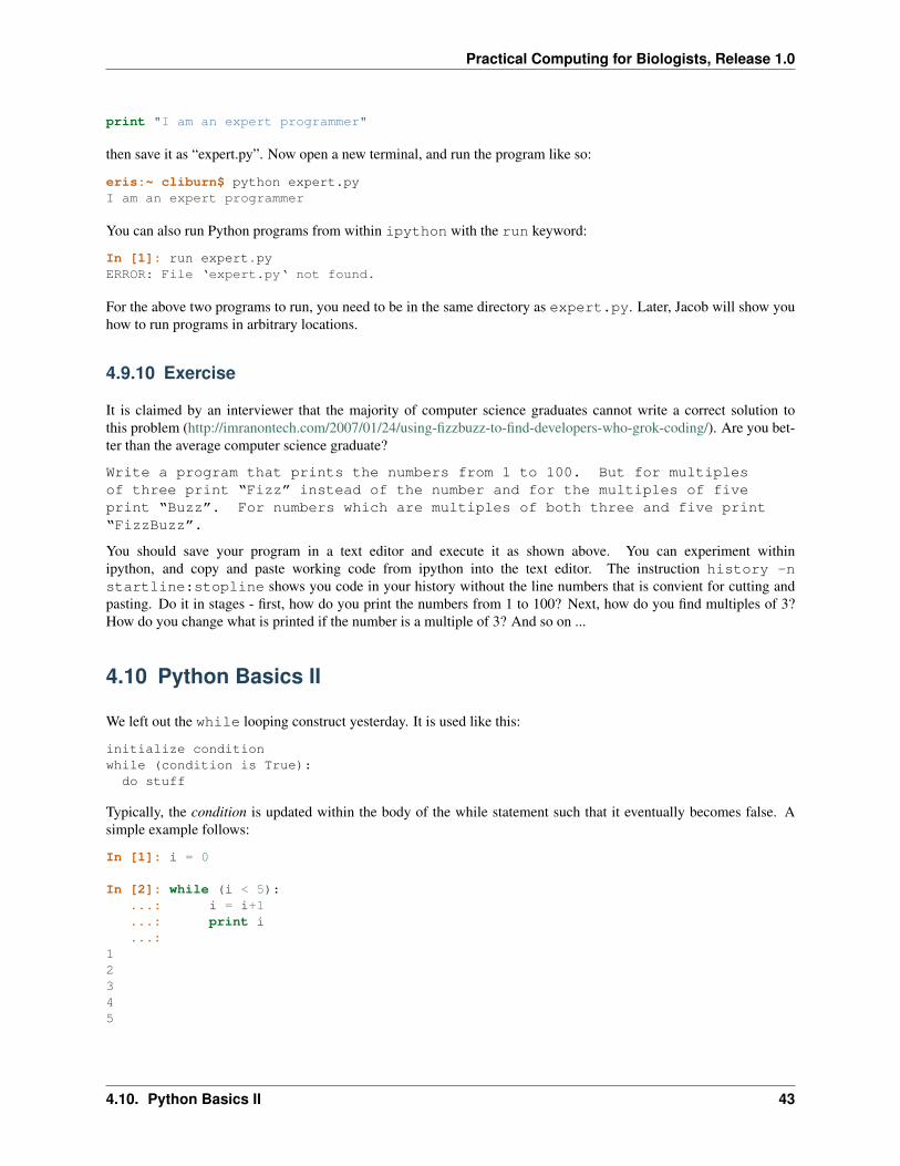
Practical Computing for Biologists, Release 1.0
print "I am an expert programmer"
then save it as “expert.py”. Now open a new terminal, and run the program like so:
eris:~ cliburn$ python expert.pyI am an expert programmer
You can also run Python programs from within ipython with the run keyword:
In [1]: run expert.pyERROR: File ‘expert.py‘ not found.
For the above two programs to run, you need to be in the same directory as expert.py. Later, Jacob will show youhow to run programs in arbitrary locations.
4.9.10 Exercise
It is claimed by an interviewer that the majority of computer science graduates cannot write a correct solution tothis problem (http://imranontech.com/2007/01/24/using-fizzbuzz-to-find-developers-who-grok-coding/). Are you bet-ter than the average computer science graduate?
Write a program that prints the numbers from 1 to 100. But for multiplesof three print “Fizz” instead of the number and for the multiples of fiveprint “Buzz”. For numbers which are multiples of both three and five print“FizzBuzz”.
You should save your program in a text editor and execute it as shown above. You can experiment withinipython, and copy and paste working code from ipython into the text editor. The instruction history -nstartline:stopline shows you code in your history without the line numbers that is convient for cutting andpasting. Do it in stages - first, how do you print the numbers from 1 to 100? Next, how do you find multiples of 3?How do you change what is printed if the number is a multiple of 3? And so on ...
4.10 Python Basics II
We left out the while looping construct yesterday. It is used like this:
initialize conditionwhile (condition is True):
do stuff
Typically, the condition is updated within the body of the while statement such that it eventually becomes false. Asimple example follows:
In [1]: i = 0
In [2]: while (i < 5):...: i = i+1...: print i...:
12345
4.10. Python Basics II 43

Practical Computing for Biologists, Release 1.0
4.10.1 Review and warm-up exercises
1. Open a terminal. What directory are you in? List the files in your current directory. Make the fol-lowing new directories - ‘folder1/folder2/folder3’. Navidgate to folder2 and create a file “catted.txt”using cat with the words “I made this!.” Delete folder1, folder2 and folder3.
1. Open your text editor. Load the file sequence1.txt. Find the sequences that would becut by the EcoRI restriction enzyme that recognizes sequneces flanked on both sides byGAATTC.
2. Create a list of cubes for all the positive inteters less than 10 (i.e. [1,8,27,...,729]) using a)a for loop and b) a list comprehension.
3. Find all the characters that are used exactly once in the sentence ‘A person who nevermade a mistake never tried anything new’. Ignore case, so ‘A’ and ‘a’ would be countedas 2 occurrences of ‘a’.
4. Find the second largest number in this list [ 9, 61, 2, 79, 58, 87, 68, 83, 61, 13]
5. Make a dictionary from these two lists, using the author as the key and the quote as thevalue:
authors = ["Albert Einstein", "Richard Feynman", "CharlesDarwin"]
quotes = ["Any man who can drive safely while kissing apretty girl is simply not giving the kiss the attention itdeserves", "There is a computer disease that anybody who workswith computers knows about. It’s a very serious disease andit interferes completely with the work. The trouble withcomputers is that you ’play’ with them!", "I have tried latelyto read Shakespeare, and found it so intolerably dull that itnauseated me"]
1. Write a program that generates this list [0,1,2,3,4,5,5,4,3,2,1,0]. Your program shouldonly contain a single integer.
2. Write a program that uses while and raw_input and simply repeats the question “whowins?” until you type the words “you win”. Here is a session with the program in theterminal:
eris:examples cliburn$ python winner.py who wins? me who wins? cliburn who wins? some-one else who wins? you win
4.10.2 String Interpolation
We start this session by learning how to construct nicely formatted strings with holes where we want to insert variables.The most convenient way to do this in python is by string interpolation. String interpolation uses codes starting withthe % symbol as placeholders for inserting variables within the string. The codes that are most useful are:
1. %s for strings
2. %d for integers
3. %f for floats
So for example, we can have this string:
In [1]: "%s took %d courses last year and had a %f GPA" % (’Tome’, 4, 3.2)Out[1]: ’Tome took 4 courses last year and had a 3.200000 GPA’
44 Chapter 4. Instructor: Cliburn Chan, Biostatistics and Bioinformatics.
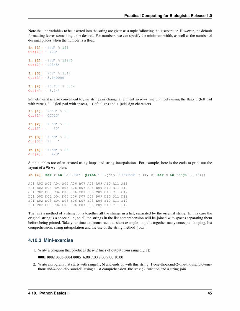
Practical Computing for Biologists, Release 1.0
Note that the variables to be inserted into the string are given as a tuple following the % separator. However, the defaultformatting leaves something to be desired. For numbers, we can specify the minimum width, as well as the number ofdecimal places when the number is a float.
In [1]: ’%4d’ % 123Out[1]: ’ 123’
In [2]: ’%4d’ % 12345Out[2]: ’12345’
In [3]: ’%5f’ % 3.14Out[3]: ’3.140000’
In [4]: ’%5.2f’ % 3.14Out[4]: ’ 3.14’
Sometimes it is also convenient to pad strings or change alignment so rows line up nicely using the flags 0 (left padwith zeros), ‘‘ ‘‘ (left pad with space), - (left align) and + (add sign character).
In [1]: ’%05d’ % 23Out[1]: ’00023’
In [2]: ’% 5d’ % 23Out[2]: ’ 23’
In [3]: ’%-5d’ % 23Out[3]: ’23 ’
In [4]: ’%+5d’ % 23Out[4]: ’ +23’
Simple tables are often created using loops and string interpolation. For example, here is the code to print out thelayout of a 96 well plate:
In [1]: for r in ’ABCDEF’: print ’ ’.join([’%s%02d’ % (r, c) for c in range(1, 13)])...:
A01 A02 A03 A04 A05 A06 A07 A08 A09 A10 A11 A12B01 B02 B03 B04 B05 B06 B07 B08 B09 B10 B11 B12C01 C02 C03 C04 C05 C06 C07 C08 C09 C10 C11 C12D01 D02 D03 D04 D05 D06 D07 D08 D09 D10 D11 D12E01 E02 E03 E04 E05 E06 E07 E08 E09 E10 E11 E12F01 F02 F03 F04 F05 F06 F07 F08 F09 F10 F11 F12
The join method of a string joins together all the strings in a list, separated by the original string. In this case theoriginal string is a space ’ ’, so all the strings in the list comprehension will be joined with spaces separating thembefore being printed. Take your time to deconstruct this short example - it pulls together many concepts - looping, listcomprehension, string interpolation and the use of the string method join.
4.10.3 Mini-exercise
1. Write a program that produces these 2 lines of output from range(1,11):
0001 0002 0003 0004 0005 6.00 7.00 8.00 9.00 10.00
2. Write a program that starts with range(1, 6) and ends up with this string ‘1-one-thousand-2-one-thousand-3-one-thousand-4-one-thousand-5’, using a list comprehension, the str() function and a string join.
4.10. Python Basics II 45
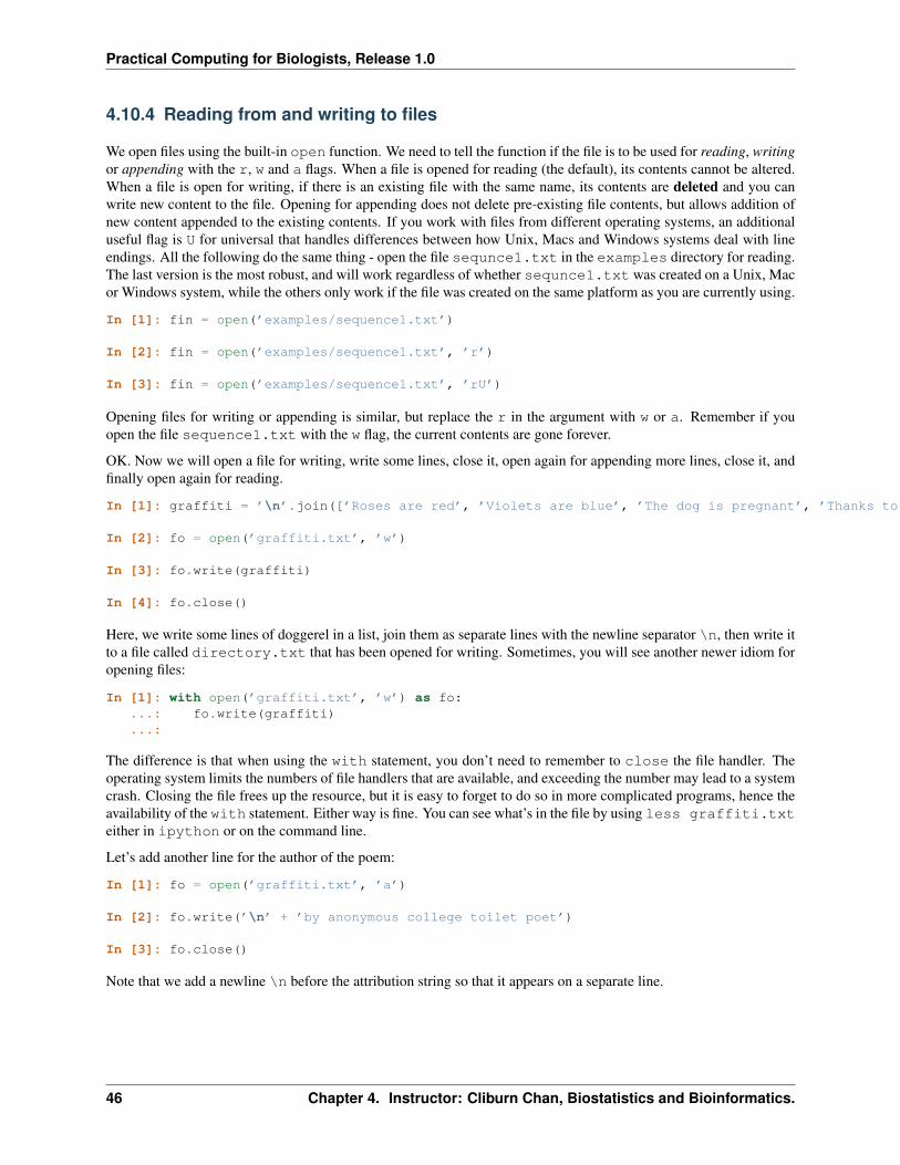
Practical Computing for Biologists, Release 1.0
4.10.4 Reading from and writing to files
We open files using the built-in open function. We need to tell the function if the file is to be used for reading, writingor appending with the r, w and a flags. When a file is opened for reading (the default), its contents cannot be altered.When a file is open for writing, if there is an existing file with the same name, its contents are deleted and you canwrite new content to the file. Opening for appending does not delete pre-existing file contents, but allows addition ofnew content appended to the existing contents. If you work with files from different operating systems, an additionaluseful flag is U for universal that handles differences between how Unix, Macs and Windows systems deal with lineendings. All the following do the same thing - open the file sequnce1.txt in the examples directory for reading.The last version is the most robust, and will work regardless of whether sequnce1.txt was created on a Unix, Macor Windows system, while the others only work if the file was created on the same platform as you are currently using.
In [1]: fin = open(’examples/sequence1.txt’)
In [2]: fin = open(’examples/sequence1.txt’, ’r’)
In [3]: fin = open(’examples/sequence1.txt’, ’rU’)
Opening files for writing or appending is similar, but replace the r in the argument with w or a. Remember if youopen the file sequence1.txt with the w flag, the current contents are gone forever.
OK. Now we will open a file for writing, write some lines, close it, open again for appending more lines, close it, andfinally open again for reading.
In [1]: graffiti = ’\n’.join([’Roses are red’, ’Violets are blue’, ’The dog is pregnant’, ’Thanks to you’])
In [2]: fo = open(’graffiti.txt’, ’w’)
In [3]: fo.write(graffiti)
In [4]: fo.close()
Here, we write some lines of doggerel in a list, join them as separate lines with the newline separator \n, then write itto a file called directory.txt that has been opened for writing. Sometimes, you will see another newer idiom foropening files:
In [1]: with open(’graffiti.txt’, ’w’) as fo:...: fo.write(graffiti)...:
The difference is that when using the with statement, you don’t need to remember to close the file handler. Theoperating system limits the numbers of file handlers that are available, and exceeding the number may lead to a systemcrash. Closing the file frees up the resource, but it is easy to forget to do so in more complicated programs, hence theavailability of the with statement. Either way is fine. You can see what’s in the file by using less graffiti.txteither in ipython or on the command line.
Let’s add another line for the author of the poem:
In [1]: fo = open(’graffiti.txt’, ’a’)
In [2]: fo.write(’\n’ + ’by anonymous college toilet poet’)
In [3]: fo.close()
Note that we add a newline \n before the attribution string so that it appears on a separate line.
46 Chapter 4. Instructor: Cliburn Chan, Biostatistics and Bioinformatics.

Practical Computing for Biologists, Release 1.0
4.10.5 Mini-exercise
1. Find the AT/GC ratio in sequence1.txt.
2. Find all palindromes of length = 9 in sequence1.txt and save them to a file called palindromes.txt.
3. Now, re-open palindromes.txt and append all palindromes of length 8 to the file.
4.10.6 Reading files with read() and readlines()
We can also store the contents of the file read in by using the read and readlines methods for further processinglater. The difference is that read returns the content as a single string, while readlines returns it as a list of lines.
In [1]: poem = open(’graffiti.txt’, ’rU’).read()
In [2]: poemOut[2]: ’Roses are red\nViolets are blue\nThe dog is pregnant\nThanks to you\nby anonymous college toilet poet’
In [3]: poem = open(’graffiti.txt’, ’rU’).readlines()
In [4]: poemOut[4]:[’Roses are red\n’,’Violets are blue\n’,’The dog is pregnant\n’,’Thanks to you\n’,’by anonymous college toilet poet’]
We can now process the string in poem1 or the list in poem2 as necessary.
4.10.7 Exercise
1. Convert the contents of the file ‘graffit.txt’ to all uppercase letters. That is, calling cat or less on graffit.txtshould look like this before and after your program is run:
BEFORE
eris:pcfb cliburn$ cat graffiti.txtRoses are redViolets are blueThe dog is pregnantThanks to youby anonymous college toilet poet
AFTER
eris:pcfb cliburn$ cat graffit.txtROSES ARE REDVIOLETS ARE BLUETHE DOG IS PREGNANTTHANKS TO YOUBY ANONYMOUS COLLEGE TOILET POETeris:pcfb cliburn$
2. Count the number of times each word appears in hamlet.txt found in theexamples folder. For, we define a word to be any string of charactersthat is separated by white space (space, tab, newline). We also ignore
4.10. Python Basics II 47

Practical Computing for Biologists, Release 1.0
case - so ’ABC’ is the same word as ’abc’. For extra credit, strip allpunctuation before doing the word count.
1. Open the file ‘hamlet.txt’ and assign its contents to a variable as a single string
2. Convert the string to lower case
3. Remove all punctuation characters from the string (punctuation characters are ‘!”#$%&’()*+,-./:;<=>?@[\]^_‘{|}~’, which you can also find in the string module)
4. Split the string into a list of words, where a word is defined to be any sequence of characters separated by whitespace
5. Create an empty dictionary to store word counts
6. Loop over the list of words and increment the dictionary count for that word by 1
7. Print the number of occurrences of ‘hamlet’ in ‘Hamlet’
8. Close the file if necessary
4.10.8 Writing your own functions
We are finally in the home stretch for the Python programming module. Learning to write your own functions willgreatly increase the complexity of the programs that you can write. A function is a black box - it takes some input,does something with it, and spits out some output. Functions hide details away, allowing you to solve problems at ahigher level without getting bogged down. For example, consider the built-in sum function:
In [1]: numbers = [1,6,23,8,1,2,90]
In [2]: sum(numbers)Out[2]: 131
The use of the built-in sum function hides the details of having to initialize the sum to zero and looping over eachnumber while adding that number to the sum variable. While Python comes with many useful built-in functions, sooneror later, you will need to write your own functions. As you will see, writing your own functions is really simple. Let’swrite our version of the sum function and a product function that when given a sequence of numbers, returns theproduct rather than the sum of numbers. We will store save the functions in examples/functions.py.
def sum(xs):"""Given a sequence of numbers, return the sum."""s = 0for x in xs:
s += xreturn s
def prod(xs):"""Given a sequence of numbers, return the product."""s = 1for x in xs:
s *= xreturn s
A typical function looks like this:
def function_name(function_arguments):"""Optional string describing the function."""statements ...return result
48 Chapter 4. Instructor: Cliburn Chan, Biostatistics and Bioinformatics.
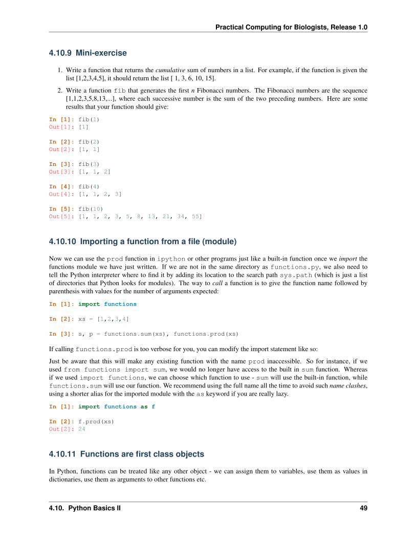
Practical Computing for Biologists, Release 1.0
4.10.9 Mini-exercise
1. Write a function that returns the cumulative sum of numbers in a list. For example, if the function is given thelist [1,2,3,4,5], it should return the list [ 1, 3, 6, 10, 15].
2. Write a function fib that generates the first n Fibonacci numbers. The Fibonacci numbers are the sequence[1,1,2,3,5,8,13,...], where each successive number is the sum of the two preceding numbers. Here are someresults that your function should give:
In [1]: fib(1)Out[1]: [1]
In [2]: fib(2)Out[2]: [1, 1]
In [3]: fib(3)Out[3]: [1, 1, 2]
In [4]: fib(4)Out[4]: [1, 1, 2, 3]
In [5]: fib(10)Out[5]: [1, 1, 2, 3, 5, 8, 13, 21, 34, 55]
4.10.10 Importing a function from a file (module)
Now we can use the prod function in ipython or other programs just like a built-in function once we import thefunctions module we have just written. If we are not in the same directory as functions.py, we also need totell the Python interpreter where to find it by adding its location to the search path sys.path (which is just a listof directories that Python looks for modules). The way to call a function is to give the function name followed byparenthesis with values for the number of arguments expected:
In [1]: import functions
In [2]: xs = [1,2,3,4]
In [3]: s, p = functions.sum(xs), functions.prod(xs)
If calling functions.prod is too verbose for you, you can modify the import statement like so:
Just be aware that this will make any existing function with the name prod inaccessible. So for instance, if weused from functions import sum, we would no longer have access to the built in sum function. Whereasif we used import functions, we can choose which function to use - sum will use the built-in function, whilefunctions.sum will use our function. We recommend using the full name all the time to avoid such name clashes,using a shorter alias for the imported module with the as keyword if you are really lazy.
In [1]: import functions as f
In [2]: f.prod(xs)Out[2]: 24
4.10.11 Functions are first class objects
In Python, functions can be treated like any other object - we can assign them to variables, use them as values indictionaries, use them as arguments to other functions etc.
4.10. Python Basics II 49

Practical Computing for Biologists, Release 1.0
In [1]: foo = functions.sum
In [2]: foo([1,2,3])Out[2]: 6
In [3]: func_dict = {’plus’ : functions.sum, ’times’ : functions.prod}
In [4]: xs = [1,2,3,4]
In [5]: func_dict[’plus’](xs)Out[5]: 10
In [6]: func_dict[’times’](xs)Out[6]: 24
There is another way to write short “throwaway” functions for one-time use that is much terser using lamba or anony-mous functions:
In [1]: f = lambda x: x*x
In [2]: f(3)Out[2]: 9
This use of lambda is typically seen in the context of the built-in higher order functions (functions that take functionsas arguments) map and filter.
In [1]: filter(lambda x: x % 2==0, range(10))Out[1]: [0, 2, 4, 6, 8]
In [2]: map(lambda x: x**2, range(5))Out[2]: [0, 1, 4, 9, 16]
In general, Python programmers prefer to use defined rather than anonymous functions, and the use of list compre-hensions rather than map and filter as they are more explicit and easier to understand, but you may come acrosslambda, map and filter in books or on the web.
4.10.12 Mini-Exercise
1. Replace the filter and map functionality in the above example using list comprehension.
2. Rewrite f = lambda x: x**2 as a regular function also called f using def.
4.10.13 Function arguments
We can define functions with more than one argument, as well as give default values to the arguments. In turn, whencalling a function, we can supply the arguments either by position or by name. Arguments with default values do notneed to be supplied when calling a function, but if provided, will overwrite the default values.
In [1]: def f(a, b, c=3, d=100):...: print a, b, c, d...:
In [2]: f(1,2)1 2 3 100
In [3]: f(1,2,3,4)
50 Chapter 4. Instructor: Cliburn Chan, Biostatistics and Bioinformatics.
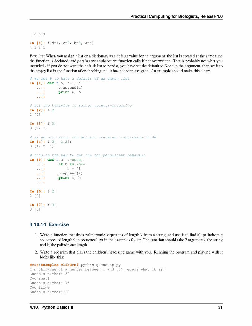
Practical Computing for Biologists, Release 1.0
1 2 3 4
In [4]: f(d=1, c=2, b=3, a=4)4 3 2 1
Warning: When you assign a list or a dictionary as a default value for an argument, the list is created at the same timethe function is declared, and persists over subsequent function calls if not overwritten. That is probably not what youintended - if you do not want the default list to persist, you have set the default to None in the argument, then set it tothe empty list in the function after checking that it has not been assigned. An example should make this clear:
# we set b to have a default of an empty listIn [1]: def f(a, b=[]):
...: b.append(a)
...: print a, b
...:
# but the behavior is rather counter-intuitiveIn [2]: f(2)2 [2]
In [3]: f(3)3 [2, 3]
# if we over-write the default argument, everything is OKIn [4]: f(3, [1,2])3 [1, 2, 3]
# this is the way to get the non-persistent behaviorIn [5]: def f(a, b=None):
...: if b is None:
...: b = []
...: b.append(a)
...: print a, b
...:
In [6]: f(2)2 [2]
In [7]: f(3)3 [3]
4.10.14 Exercise
1. Write a function that finds palindromic sequences of length k from a string, and use it to find all palindromicsequences of length 9 in sequence1.txt in the examples folder. The function should take 2 arguments, the stringand k, the palindrome length
2. Write a program that plays the children’s guessing game with you. Running the program and playing with itlooks like this:
eris:examples cliburn$ python guessing.pyI’m thinking of a number between 1 and 100. Guess what it is!Guess a number: 50Too smallGuess a number: 75Too largeGuess a number: 63
4.10. Python Basics II 51

Practical Computing for Biologists, Release 1.0
Too largeGuess a number: 56Too smallGuess a number: 60Too largeGuess a number: 58You’ve guessed it! The number is 58
The first 5 lines of the program look like this:
import random
number = random.randint(1, 101)guess = Noneprint "I’m thinking of a number between 1 and 100. Guess what it is!"while guess != number:
YOUR CODE HERE
4.11 Python Modules
Python comes with many libraries covering a large variety of functions. During this section we will look at some ofthem.
Recall that libraries are accessed using the import statement. You can see what object a library contains by usingdir(<module>) in ipython, and looking at <module>.<object>.__doc__ string
In [1]: import math
In [2]: print math.exp.__doc__exp(x)
Return e raised to the power of x.
4.11.1 os module
The os module provide a platform independent way to work with the operating system, make or remove files anddirectories.
In [1]: import os
In [2]: print os.getcwd()/home/jacob
In [3]: os.chdir(’/home/jacob/baz’)
In [4]: os.getcwd()Out[4]: ’/home/jacob/baz’
In [5]: os.remove(’foo’)
In [6]: os.chdir(’/home/jacob’)
In [7]: os.rmdir(’baz’)
52 Chapter 4. Instructor: Cliburn Chan, Biostatistics and Bioinformatics.

Practical Computing for Biologists, Release 1.0
4.11.2 csv module
The csv module provides readers and writers for comma separated value data.
In [1]: import csv
In [2]: f = open(’monty_python.csv’, ’w’)
In [3]: cfw = csv.writer(f, dialect=’excel’)
In [4]: cfw.writerow([’spam’,’spam’,’eggs’,’spam’])
In [5]: cfw.writerow([’spam’,’spam’,’spam and eggs’, ’spam’])
In [6]: cfw.writerow([’toast’])
In [7]: f.close()
In [8]: cfr = csv.reader(open(’monty_python.csv’, ’rU’), dialect=’excel’)
In [9]: for row in cfr:...: print ’, ’.join(row)...:
spam, spam, eggs, spamspam, spam, spam and eggs, spamtoast
If you’d prefer a different separator than commas the delimiter optional argument can be used
In [1]: import csv
In [2]: f = open(’tabbs.csv’, ’rU’)
In [3]: csvfile = csv.reader(f, delimiter=’\t’)
In [4]: for row in csvfile:...: print row...:
[’1’, ’2’, ’3’][’2’, ’3’, ’4’][’4’, ’5’, ’6’]
often you’ll want to skip the first row in a csv file, and a simple way to do that is
import csv
f = open(’test_scores.csv’, ’rU’)csvfile = csv.reader(f)
header = False
for row in csvfile:if not header:
header = Trueelse:
print rowf.close()
4.11. Python Modules 53
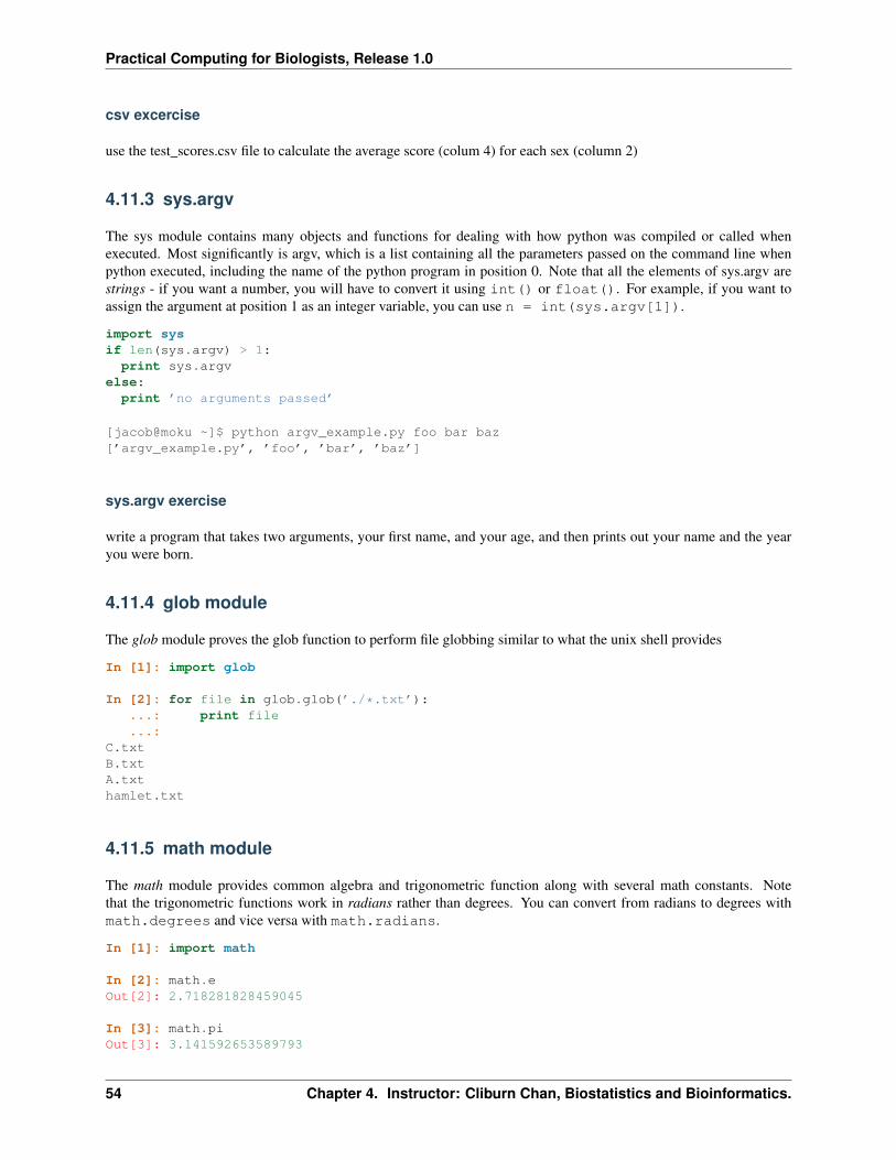
Practical Computing for Biologists, Release 1.0
csv excercise
use the test_scores.csv file to calculate the average score (colum 4) for each sex (column 2)
4.11.3 sys.argv
The sys module contains many objects and functions for dealing with how python was compiled or called whenexecuted. Most significantly is argv, which is a list containing all the parameters passed on the command line whenpython executed, including the name of the python program in position 0. Note that all the elements of sys.argv arestrings - if you want a number, you will have to convert it using int() or float(). For example, if you want toassign the argument at position 1 as an integer variable, you can use n = int(sys.argv[1]).
import sysif len(sys.argv) > 1:
print sys.argvelse:print ’no arguments passed’
[jacob@moku ~]$ python argv_example.py foo bar baz[’argv_example.py’, ’foo’, ’bar’, ’baz’]
sys.argv exercise
write a program that takes two arguments, your first name, and your age, and then prints out your name and the yearyou were born.
4.11.4 glob module
The glob module proves the glob function to perform file globbing similar to what the unix shell provides
In [1]: import glob
In [2]: for file in glob.glob(’./*.txt’):...: print file...:
C.txtB.txtA.txthamlet.txt
4.11.5 math module
The math module provides common algebra and trigonometric function along with several math constants. Notethat the trigonometric functions work in radians rather than degrees. You can convert from radians to degrees withmath.degrees and vice versa with math.radians.
In [1]: import math
In [2]: math.eOut[2]: 2.718281828459045
In [3]: math.piOut[3]: 3.141592653589793
54 Chapter 4. Instructor: Cliburn Chan, Biostatistics and Bioinformatics.
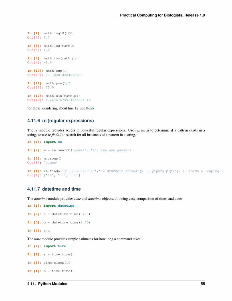
Practical Computing for Biologists, Release 1.0
In [4]: math.log10(100)Out[4]: 2.0
In [5]: math.log(math.e)Out[5]: 1.0
In [7]: math.cos(math.pi)Out[7]: -1.0
In [10]: math.exp(1)Out[10]: 2.7182818284590455
In [11]: math.pow(5,2)Out[11]: 25.0
In [12]: math.sin(math.pi)Out[12]: 1.2246467991473532e-16
for those wondering about line 12, see floats
4.11.6 re (regular expressions)
The re module provides access to powerful regular expressions. Use re.search to determine if a pattern exists in astring, or use re.findall to search for all instances of a pattern in a string.
In [1]: import re
In [2]: m = re.search(’games’, ’all fun and games’)
In [3]: m.group()Out[3]: ’games’
In [4]: re.findall(’[1234567890]+’,’12 drummers drumming, 11 pipers piping, 10 lords a-leaping’)Out[4]: [’12’, ’11’, ’10’]
4.11.7 datetime and time
The datetime module provides time and datetime objects, allowing easy comparison of times and dates.
In [1]: import datetime
In [2]: a = datetime.time(8,30)
In [3]: b = datetime.time(9,45)
In [4]: b>a
The time module provides simple estimates for how long a command takes.
In [1]: import time
In [2]: a = time.time()
In [3]: time.sleep(10)
In [4]: b = time.time()
4.11. Python Modules 55
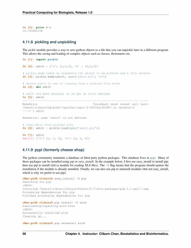
Practical Computing for Biologists, Release 1.0
In [5]: print b-a10.743445158
4.11.8 pickling and unpickling
The pickle module provides a way to save python objects to a file that you can unpickle later in a different program.This allows the saving and loading of complex objects such as classes, dictionaries etc.
In [1]: import pickle
In [2]: adict = {’a’: [1,2,3], ’b’ : [4,5,6]}
# pickle.dump takes as arguments the object to be pickled and a file handlerIn [3]: pickle.dump(adict, open(’adict.pic’, ’w’))
# delete adict to see if loading from a pickled file worksIn [4]: del adict
# adict has been deleted, so we get an error messageIn [5]: adict---------------------------------------------------------------------------NameError Traceback (most recent call last)/Users/cliburn/hg/pcfb/<ipython-input-5-5f470a13239f> in <module>()----> 1 adict
NameError: name ’adict’ is not defined
# load adict from pickled fileIn [6]: adict = pickle.load(open(’adict.pic’))
In [7]: adictOut[7]: {’a’: [1, 2, 3], ’b’: [4, 5, 6]}
4.11.9 pypi (formerly cheese shop)
The python community maintains a database of third party python packages. This database lives at pypi. Many ofthese packages can be installed using pip or easy_install. In the example below, I first use easy_install to install pip,then use pip to install xlrd (a module for reading XLS files). The -U flag means that the program should update theinstallation if the module is already installed. Finally, we can also use pip to uninstall modules (but not easy_install,which is why we prefer to use pip).
iMac:pcfb cliburn$ easy_install -U pipSearching for pip<SNIP>Installed /Users/cliburn/Library/Python/2.7/site-packages/pip-1.1-py2.7.eggProcessing dependencies for pipFinished processing dependencies for pip
iMac:pcfb cliburn$ pip install -U xlrdDownloading/unpacking xlrd from<SNIP>Successfully installed xlrdCleaning up...
iMac:pcfb cliburn$ pip uninstall xlrd
56 Chapter 4. Instructor: Cliburn Chan, Biostatistics and Bioinformatics.

Practical Computing for Biologists, Release 1.0
Uninstalling xlrd:/Users/cliburn/Library/Python/2.7/site-packages/xlrd/Users/cliburn/Library/Python/2.7/site-packages/xlrd-0.7.7-py2.7.egg-info/Users/cliburn/bin/runxlrd.py
Proceed (y/n)? ySuccessfully uninstalled xlrd
4.11.10 Exercise
Write a program that takes a number on the command line and calculates the log, square, sin and cosine, and writesthem out in a csv file.
4.12 NumPy and Matplotlib
4.12.1 NumPy - numeric computing
NumPy is the de facto standard for numerical computing in Python. It is highly optimized and extremely usefulfor working with matrices. The standard matrix class in NumPy is called an array. We will first get comfortablewith working with arrays the we will cover a number of useful functions. Then we will touch on the linear algebracapabilities of NumPy and finally we will use a few examples to tie together key concepts.
NumPy - arrays
Contents
The main object in NumPy is the homogeneous, multidimensional array. An array is a table of elements. An exampleis a matrix x
x =
1 2 34 5 67 8 9
can be represented as
>>> import numpy as np>>> x = np.array([[1,2,3],[4,5,6],[7,8,9]])>>> xarray([[1, 2, 3],
[4, 5, 6],[7, 8, 9]])
>>> x.shape(3, 3)
The array x has 2 dimensions. In NumPy the number of dimensions is referred to as rank. The ndim is the same asthe number of axes or the length of the output of x.shape
>>> x.ndim2
>>> x.size9
Arrays are convenient because of built in methods.
4.12. NumPy and Matplotlib 57

Practical Computing for Biologists, Release 1.0
>>> x.sum(axis=0)array([12, 15, 18])>>> x.sum(axis=1)array([ 6, 15, 24])
>>> x.mean(axis=0)array([ 4., 5., 6.])>>> x.mean(axis=1)array([ 2., 5., 8.])
But arrays are also useful because they interact with other NumPy functions as well as being central to other packagefunctionality. To make a sequence of numbers, similar to range in the Python standard library, we use arange.
>>> np.arange(10)array([0, 1, 2, 3, 4, 5, 6, 7, 8, 9])>>> np.arange(5,10)array([5, 6, 7, 8, 9])>>> np.arange(5,10,0.5)array([ 5. , 5.5, 6. , 6.5, 7. , 7.5, 8. , 8.5, 9. , 9.5])
Also we can recreate the first matrix by reshaping the output of arange.
>>> x = np.arange(1,10).reshape(3,3)>>> xarray([[1, 2, 3],
[4, 5, 6],[7, 8, 9]])
Another similar function to arange is linspace which fills a vector with evenly spaced variables for a specified interval.
>>> x = np.linspace(0,5,5)>>> xarray([ 0. , 1.25, 2.5 , 3.75, 5. ])
As a reminder you may access the documentation at anytime using
~$ pydoc numpy.linspace
Visualizing linspace...
import numpy as npimport matplotlib.pyplot as pltfig = plt.figure()ax = fig.add_subplot(111)N = 8y = np.zeros(N)x1 = np.linspace(0, 10, N, endpoint=True)p1 = plt.plot(x1, y, ’o’)ax.set_xlim([-0.5,10.5])plt.show()
58 Chapter 4. Instructor: Cliburn Chan, Biostatistics and Bioinformatics.

Practical Computing for Biologists, Release 1.0
0 2 4 6 8 100.06
0.04
0.02
0.00
0.02
0.04
0.06
Arrays may be made of different types of data.
>>> x = np.array([1,2,3])>>> x.dtypedtype(’int64’)>>> x = np.array([0.1,0.2,0.3])>>> xarray([ 0.1, 0.2, 0.3])>>> x.dtypedtype(’float64’)>>> x = np.array([1,2,3],dtype=’float64’)>>> x.dtypedtype(’float64’)
There are several convenience functions for making arrays that are worth mentioning:
• zeros
• ones
>>> x = np.zeros([3,4])>>> xarray([[ 0., 0., 0., 0.],
[ 0., 0., 0., 0.],[ 0., 0., 0., 0.]])
>>> x = np.ones([3,4])>>> x
4.12. NumPy and Matplotlib 59

Practical Computing for Biologists, Release 1.0
array([[ 1., 1., 1., 1.],[ 1., 1., 1., 1.],[ 1., 1., 1., 1.]])
Exercise
1. Create the following array (1 line)
a =
1 2 · · · 1011 12 · · · 20...
. . . . . ....
91 92 · · · 100
2. Use the array object to get the number of elements, rows and columns
3. Get the mean of the rows and columns
4. What do you get when you do this?
>>> a[4,:]
5. [extra] If you have time you can get familiar try
• np.log(a)
• np.cumsum(a)
• np.rank(a)
• np.power(a,2)
6. [extra] How do you create a vector that has exactly 50 points and spans the range 11 to 23
NumPy - basics
Quick reference
Here we provide a quick reference guide to the commonly used functions from the NumPy package along with severalfrequently encountered examples.
NumPy command Notea.ndim returns the num. of dimensionsa.shape returns the num. of rows and columsarange(start,stop,step) returns a sequence vectorlinspace(start,stop,steps) returns a evenly spaced sequence in the specificed intervaldot(a,b) matrix multiplicationvstack([a,b]) stack arrays a and b verticallyhstack([a,b]) stack arrays a and b horizontallywhere(a>x) returns elements from an array depending on conditionargsort(a) returns the sorted indices of an input array
Basic operations
Arithmetic operators in NumPy work elementwise.
60 Chapter 4. Instructor: Cliburn Chan, Biostatistics and Bioinformatics.

Practical Computing for Biologists, Release 1.0
>>> a = np.array([3,4,5])>>> b = np.ones(3)>>> a - barray([ 2., 3., 4.])
Something that can be tricky for people familar with other programming languages is that the * operator does notcarry out a matrix product. This is done with the dot function.
>>> a = np.array([[1,2],[3,4]])>>> b = np.array([[1,2],[3,4]])>>> aarray([[1, 2],
[3, 4]])>>> barray([[1, 2],
[3, 4]])>>> a * barray([[ 1, 4],
[ 9, 16]])>>> np.dot(a,b)array([[ 7, 10],
[15, 22]])
Special addition and multiplication operators>>> a = np.zeros((2,2),dtype=’float’)>>> a += 5>>> aarray([[ 5., 5.],
[ 5., 5.]])>>> a *= 5>>> aarray([[ 25., 25.],
[ 25., 25.]])>>> a + aarray([[ 50., 50.],
[ 50., 50.]])
Concatenation>>> a = np.array([1,2,3])>>> b = np.array([4,5,6])>>> c = np.array([7,8,9])>>> np.hstack([a,b,c])array([1, 2, 3, 4, 5, 6, 7, 8, 9])>>> np.vstack([a,b,c])array([[1, 2, 3],
[4, 5, 6],[7, 8, 9]])
Sorting arrays>>> x.sort()>>> xarray([0, 0, 1, 3, 4, 5])>>> x = np.array(([1,3,4,0,0,5]))array([3, 4, 0, 1, 2, 5])
4.12. NumPy and Matplotlib 61

Practical Computing for Biologists, Release 1.0
>>> np.argsort(x)array([3, 4, 0, 1, 2, 5])
Common math functions>>> x = np.arange(1,5)>>> np.sqrt(x) * np.piarray([ 3.14159265, 4.44288294, 5.44139809, 6.28318531])>>> 2**416>>> np.power(2,4)16>>> np.log(np.e)1.0>>> x = np.arange(5)>>> x.max() - x.min()4
Basic operations excerciseExercise
In the following table we have expression values for 5 genes at 4 time points. These are completely made up data.Although, some of the questions can be easily answered by looking at the data, microarray data generally come inmuch larger tables and if you can figure it out here the same code will work for an entire gene chip.
Gene name 4h 12h 24h 48hA2M 0.12 0.08 0.06 0.02FOS 0.01 0.07 0.11 0.09BRCA2 0.03 0.04 0.04 0.02CPOX 0.05 0.09 0.11 0.14
1. create a single array for the data (4x4)
2. find the mean expression value per gene
3. find the mean expression value per time point
4. which gene has the maximum mean expression value?
5. sort the gene names by the max expression value
Tip:
>>> geneList = np.array(["A2M", "FOS", "BRCA2","CPOX"])>>> values0 = np.array([0.12,0.08,0.06,0.02])>>> values1 = np.array([0.01,0.07,0.11,0.09])>>> values2 = np.array([0.03,0.04,0.04,0.02])>>> values3 = np.array([0.05,0.09,0.11,0.14])
Additional NumPy
Indexing and Slicing 1D arrays can be indexed in the same way a Python list can.
62 Chapter 4. Instructor: Cliburn Chan, Biostatistics and Bioinformatics.

Practical Computing for Biologists, Release 1.0
>>> a = np.arange(10)>>> a[2:4]array([2, 3])>>> a[:10:2]array([0, 2, 4, 6, 8])>>> a[::-1]array([9, 8, 7, 6, 5, 4, 3, 2, 1, 0])
Multidimensional arrays can have one index per axis
>>> x = np.arange(12).reshape(3,4)>>> xarray([[ 0, 1, 2, 3],
[ 4, 5, 6, 7],[ 8, 9, 10, 11]])
>>> x[2,3]11>>> x[:,1] # everything in the second rowarray([1, 5, 9])>>> x[1,:] # everything in the second columnarray([4, 5, 6, 7])>>> x[1:3,:] # second and third rowsarray([[ 4, 5, 6, 7],
[ 8, 9, 10, 11]])
Where>>> a = np.array([1,1,1,2,2,2,3,3,3])>>> a[a>1]array([2, 2, 2, 3, 3, 3])>>> a[a==3]array([3, 3, 3])>>> np.where(a<3)(array([0, 1, 2, 3, 4, 5]),)>>> np.where(a<3)[0]array([0, 1, 2, 3, 4, 5])>>> np.where(a>9)(array([], dtype=int64),)
Printing>>> for row in x:... print row...[0 1 2 3][4 5 6 7][ 8 9 10 11]
>>> for element in x.flat:... print element...0123456
4.12. NumPy and Matplotlib 63
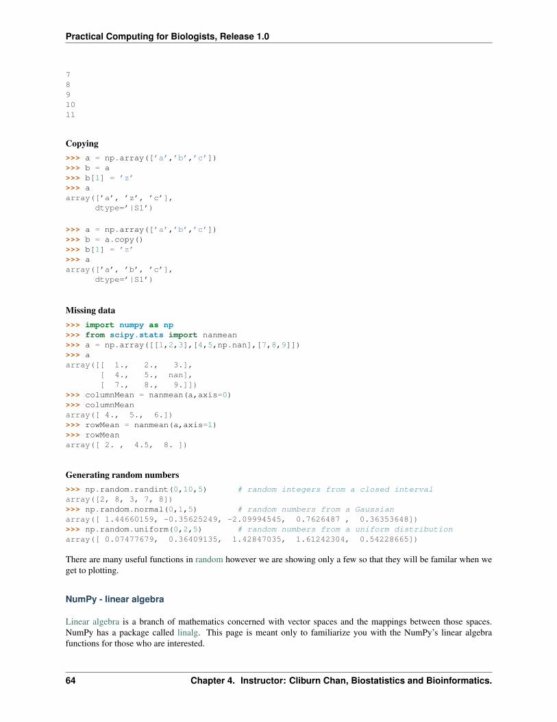
Practical Computing for Biologists, Release 1.0
7891011
Copying>>> a = np.array([’a’,’b’,’c’])>>> b = a>>> b[1] = ’z’>>> aarray([’a’, ’z’, ’c’],
dtype=’|S1’)
>>> a = np.array([’a’,’b’,’c’])>>> b = a.copy()>>> b[1] = ’z’>>> aarray([’a’, ’b’, ’c’],
dtype=’|S1’)
Missing data>>> import numpy as np>>> from scipy.stats import nanmean>>> a = np.array([[1,2,3],[4,5,np.nan],[7,8,9]])>>> aarray([[ 1., 2., 3.],
[ 4., 5., nan],[ 7., 8., 9.]])
>>> columnMean = nanmean(a,axis=0)>>> columnMeanarray([ 4., 5., 6.])>>> rowMean = nanmean(a,axis=1)>>> rowMeanarray([ 2. , 4.5, 8. ])
Generating random numbers>>> np.random.randint(0,10,5) # random integers from a closed intervalarray([2, 8, 3, 7, 8])>>> np.random.normal(0,1,5) # random numbers from a Gaussianarray([ 1.44660159, -0.35625249, -2.09994545, 0.7626487 , 0.36353648])>>> np.random.uniform(0,2,5) # random numbers from a uniform distributionarray([ 0.07477679, 0.36409135, 1.42847035, 1.61242304, 0.54228665])
There are many useful functions in random however we are showing only a few so that they will be familar when weget to plotting.
NumPy - linear algebra
Linear algebra is a branch of mathematics concerned with vector spaces and the mappings between those spaces.NumPy has a package called linalg. This page is meant only to familiarize you with the NumPy’s linear algebrafunctions for those who are interested.
64 Chapter 4. Instructor: Cliburn Chan, Biostatistics and Bioinformatics.

Practical Computing for Biologists, Release 1.0
A 1×N dimensional vector x
x =
x1
x2
...xN
and its transpose xT = (x1, x2, . . . , xN ) can be expressed in python as
>>> import numpy as np>>> x = np.array([[1,2,3]]).T>>> xt = x.T>>> x.shape(3, 1)>>> xt.shape(1, 3)
A column matrix in NumPy.
x =
3456
>>> x = np.array([[3,4,5,6]]).T
A row matrix in NumPy.
x =(3 4 5 6
)
>>> x = np.array([[3,4,5,6]])
General matrices you are already familiar with.
Am,n =
a1,1 a1,2 · · · a1,na2,1 a2,2 · · · a2,n
......
. . ....
am,1 am,2 · · · am,n
Common tasks
Matrix determinant>>> a = np.array([[3,-9],[2,5]])>>> np.linalg.det(a)33.000000000000014
Matrix inverse>>> A = np.array([[-4,-2],[5,5]])>>> Aarray([[-4, -2],
[ 5, 5]])>>> invA = np.linalg.inv(A)
4.12. NumPy and Matplotlib 65
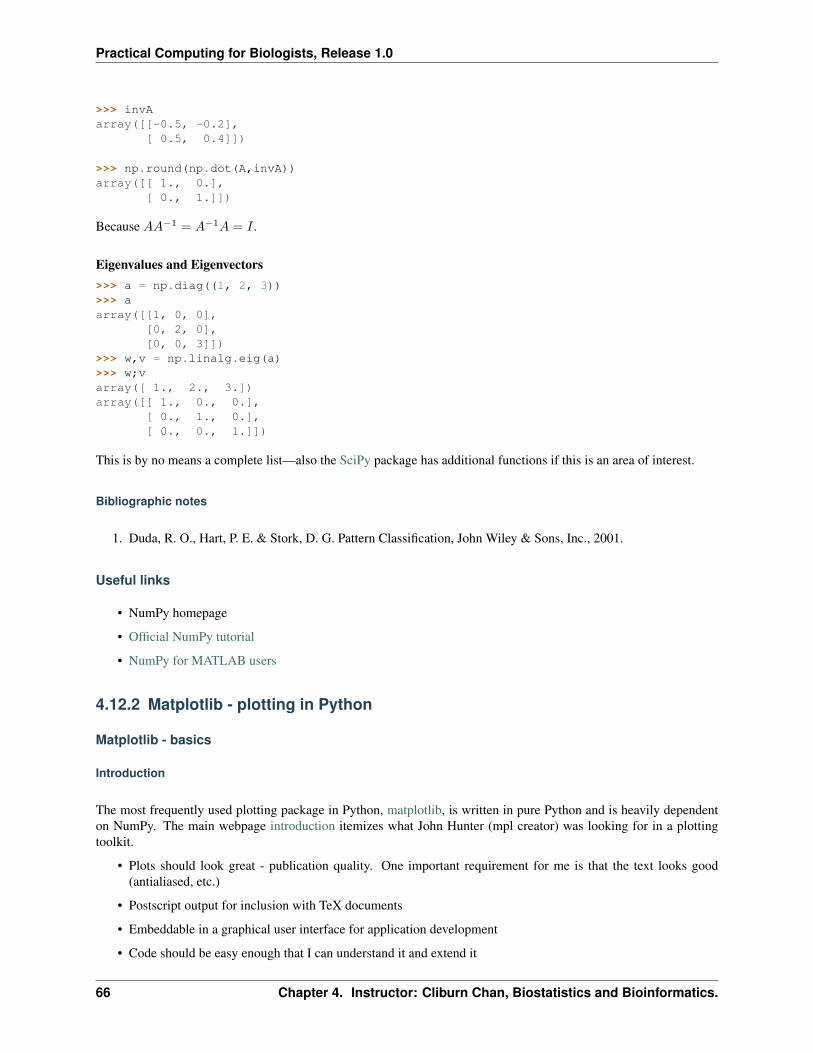
Practical Computing for Biologists, Release 1.0
>>> invAarray([[-0.5, -0.2],
[ 0.5, 0.4]])
>>> np.round(np.dot(A,invA))array([[ 1., 0.],
[ 0., 1.]])
Because AA−1 = A−1A = I .
Eigenvalues and Eigenvectors>>> a = np.diag((1, 2, 3))>>> aarray([[1, 0, 0],
[0, 2, 0],[0, 0, 3]])
>>> w,v = np.linalg.eig(a)>>> w;varray([ 1., 2., 3.])array([[ 1., 0., 0.],
[ 0., 1., 0.],[ 0., 0., 1.]])
This is by no means a complete list—also the SciPy package has additional functions if this is an area of interest.
Bibliographic notes
1. Duda, R. O., Hart, P. E. & Stork, D. G. Pattern Classification, John Wiley & Sons, Inc., 2001.
Useful links
• NumPy homepage
• Official NumPy tutorial
• NumPy for MATLAB users
4.12.2 Matplotlib - plotting in Python
Matplotlib - basics
Introduction
The most frequently used plotting package in Python, matplotlib, is written in pure Python and is heavily dependenton NumPy. The main webpage introduction itemizes what John Hunter (mpl creator) was looking for in a plottingtoolkit.
• Plots should look great - publication quality. One important requirement for me is that the text looks good(antialiased, etc.)
• Postscript output for inclusion with TeX documents
• Embeddable in a graphical user interface for application development
• Code should be easy enough that I can understand it and extend it
66 Chapter 4. Instructor: Cliburn Chan, Biostatistics and Bioinformatics.
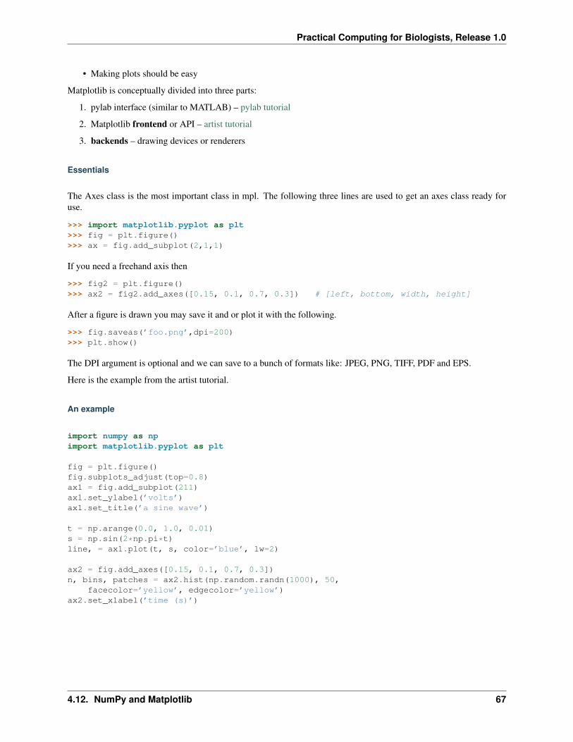
Practical Computing for Biologists, Release 1.0
• Making plots should be easy
Matplotlib is conceptually divided into three parts:
1. pylab interface (similar to MATLAB) – pylab tutorial
2. Matplotlib frontend or API – artist tutorial
3. backends – drawing devices or renderers
Essentials
The Axes class is the most important class in mpl. The following three lines are used to get an axes class ready foruse.
>>> import matplotlib.pyplot as plt>>> fig = plt.figure()>>> ax = fig.add_subplot(2,1,1)
If you need a freehand axis then
>>> fig2 = plt.figure()>>> ax2 = fig2.add_axes([0.15, 0.1, 0.7, 0.3]) # [left, bottom, width, height]
After a figure is drawn you may save it and or plot it with the following.
>>> fig.saveas(’foo.png’,dpi=200)>>> plt.show()
The DPI argument is optional and we can save to a bunch of formats like: JPEG, PNG, TIFF, PDF and EPS.
Here is the example from the artist tutorial.
An example
import numpy as npimport matplotlib.pyplot as plt
fig = plt.figure()fig.subplots_adjust(top=0.8)ax1 = fig.add_subplot(211)ax1.set_ylabel(’volts’)ax1.set_title(’a sine wave’)
t = np.arange(0.0, 1.0, 0.01)s = np.sin(2*np.pi*t)line, = ax1.plot(t, s, color=’blue’, lw=2)
ax2 = fig.add_axes([0.15, 0.1, 0.7, 0.3])n, bins, patches = ax2.hist(np.random.randn(1000), 50,
facecolor=’yellow’, edgecolor=’yellow’)ax2.set_xlabel(’time (s)’)
4.12. NumPy and Matplotlib 67

Practical Computing for Biologists, Release 1.0
0.0 0.2 0.4 0.6 0.8 1.01.0
0.5
0.0
0.5
1.0
volt
s
a sine wave
4 3 2 1 0 1 2 3 4time (s)
0
10
20
30
40
50
60
Matplotlib - line and box plots
• Simple line plot
• Lines with markers
• Box plots
Simple line plot
import numpy as npimport matplotlib.pyplot as plt
## initialize the axesfig = plt.figure()ax = fig.add_subplot(111)
## format axesax.set_ylabel(’volts’)ax.set_title(’a sine wave’)
t = np.arange(0.0, 1.0, 0.01)s = np.sin(2*np.pi*t)line, = ax.plot(t, s, color=’blue’, lw=2)
68 Chapter 4. Instructor: Cliburn Chan, Biostatistics and Bioinformatics.

Practical Computing for Biologists, Release 1.0
0.0 0.2 0.4 0.6 0.8 1.01.0
0.5
0.0
0.5
1.0volt
sa sine wave
Lines with markers
import numpy as npimport matplotlib.pyplot as plt
## initialize the figurefig = plt.figure()
## the datat = np.arange(0.0, 1.0, 0.01)s = np.sin(2*np.pi*t)
## the top axesax1 = fig.add_subplot(3,1,1)ax1.set_ylabel(’volts’)ax1.set_title(’a sine wave’)
line1 = ax1.plot(t, s+5.0, color=’blue’, lw=2)line2 = ax1.plot(t, s+2.5, color=’red’, lw=2)line3 = ax1.plot(t, s, color=’orange’, lw=2)
## the middle axesax2 = fig.add_subplot(3,1,2)
4.12. NumPy and Matplotlib 69
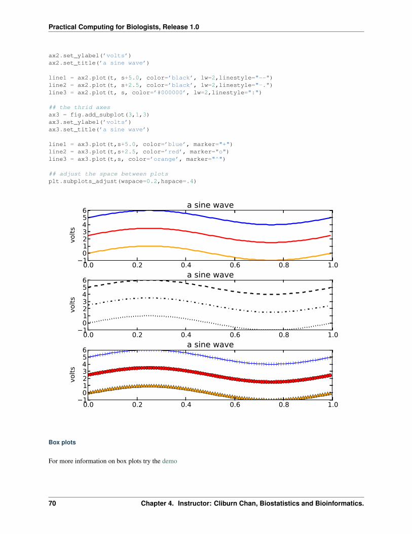
Practical Computing for Biologists, Release 1.0
ax2.set_ylabel(’volts’)ax2.set_title(’a sine wave’)
line1 = ax2.plot(t, s+5.0, color=’black’, lw=2,linestyle="--")line2 = ax2.plot(t, s+2.5, color=’black’, lw=2,linestyle="-.")line3 = ax2.plot(t, s, color=’#000000’, lw=2,linestyle=":")
## the thrid axesax3 = fig.add_subplot(3,1,3)ax3.set_ylabel(’volts’)ax3.set_title(’a sine wave’)
line1 = ax3.plot(t,s+5.0, color=’blue’, marker="+")line2 = ax3.plot(t,s+2.5, color=’red’, marker="o")line3 = ax3.plot(t,s, color=’orange’, marker="^")
## adjust the space between plotsplt.subplots_adjust(wspace=0.2,hspace=.4)
0.0 0.2 0.4 0.6 0.8 1.010123456
volt
s
a sine wave
0.0 0.2 0.4 0.6 0.8 1.010123456
volt
s
a sine wave
0.0 0.2 0.4 0.6 0.8 1.010123456
volt
s
a sine wave
Box plots
For more information on box plots try the demo
70 Chapter 4. Instructor: Cliburn Chan, Biostatistics and Bioinformatics.
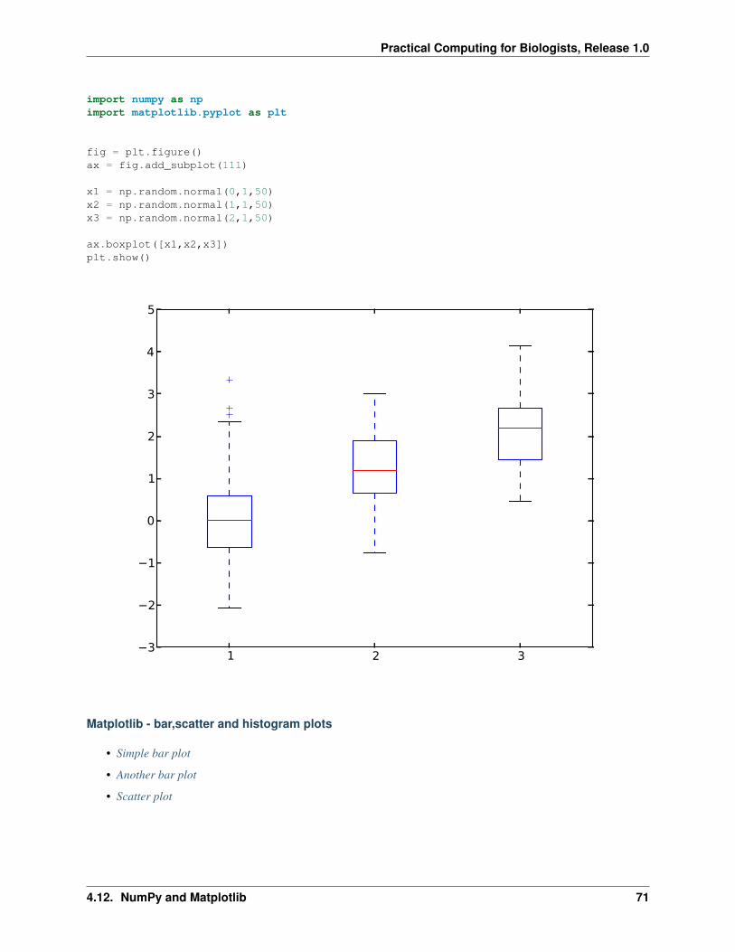
Practical Computing for Biologists, Release 1.0
import numpy as npimport matplotlib.pyplot as plt
fig = plt.figure()ax = fig.add_subplot(111)
x1 = np.random.normal(0,1,50)x2 = np.random.normal(1,1,50)x3 = np.random.normal(2,1,50)
ax.boxplot([x1,x2,x3])plt.show()
1 2 33
2
1
0
1
2
3
4
5
Matplotlib - bar,scatter and histogram plots
• Simple bar plot
• Another bar plot
• Scatter plot
4.12. NumPy and Matplotlib 71

Practical Computing for Biologists, Release 1.0
Simple bar plot
import numpy as npimport matplotlib.pyplot as plt
fig = plt.figure()ax = fig.add_subplot(111)
## the dataN = 5menMeans = [18, 35, 30, 35, 27]menStd = [2, 3, 4, 1, 2]womenMeans = [25, 32, 34, 20, 25]womenStd = [3, 5, 2, 3, 3]
## necessary variablesind = np.arange(N) # the x locations for the groupswidth = 0.35 # the width of the bars
## the barsrects1 = ax.bar(ind, menMeans, width,
color=’black’,yerr=menStd,error_kw=dict(elinewidth=2,ecolor=’red’))
rects2 = ax.bar(ind+width, womenMeans, width,color=’red’,yerr=womenStd,error_kw=dict(elinewidth=2,ecolor=’black’))
# axes and labelsax.set_xlim(-width,len(ind)+width)ax.set_ylim(0,45)ax.set_ylabel(’Scores’)ax.set_title(’Scores by group and gender’)xTickMarks = [’Group’+str(i) for i in range(1,6)]ax.set_xticks(ind+width)xtickNames = ax.set_xticklabels(xTickMarks)plt.setp(xtickNames, rotation=45, fontsize=10)
## add a legendax.legend( (rects1[0], rects2[0]), (’Men’, ’Women’) )
plt.show()
72 Chapter 4. Instructor: Cliburn Chan, Biostatistics and Bioinformatics.

Practical Computing for Biologists, Release 1.0
Group
1
Group
2
Group
3
Group
4
Group
50
5
10
15
20
25
30
35
40
45Sco
res
Scores by group and gender
MenWomen
Another bar plot
from mpl_toolkits.mplot3d import Axes3Dimport matplotlib.pyplot as pltimport numpy as np
fig = plt.figure()ax = fig.add_subplot(111,projection=’3d’)for c, z in zip([’r’, ’g’, ’b’, ’y’], [30, 20, 10, 0]):
xs = np.arange(20)ys = np.random.rand(20)
# You can provide either a single color or an array. To demonstrate this,# the first bar of each set will be colored cyan.cs = [c] * len(xs)cs[0] = ’c’ax.bar(xs, ys, zs=z, zdir=’y’, color=cs, alpha=0.8)
ax.set_xlabel(’X’)ax.set_ylabel(’Y’)ax.set_zlabel(’Z’)
plt.show()
4.12. NumPy and Matplotlib 73

Practical Computing for Biologists, Release 1.0
X
05
1015
Y
05
1015
2025
30
Z
0.0
0.2
0.4
0.6
0.8
Scatter plot
#!/usr/bin/env pythonimport matplotlib.pyplot as pltimport numpy as np
fig = plt.figure()ax1 = fig.add_subplot(121)
## the dataN=1000x = np.random.randn(N)y = np.random.randn(N)
## left panelax1.scatter(x,y,color=’blue’,s=5,edgecolor=’none’)ax1.set_aspect(1./ax1.get_data_ratio()) # make axes square
## right panelax2 = fig.add_subplot(122)props = dict(alpha=0.5, edgecolors=’none’ )
handles = []
74 Chapter 4. Instructor: Cliburn Chan, Biostatistics and Bioinformatics.

Practical Computing for Biologists, Release 1.0
colors = [’blue’, ’green’, ’magenta’, ’cyan’]for color in colors:
x = np.random.randn(N)y = np.random.randn(N)s = np.random.randint(50,200)handles.append(ax2.scatter(x, y, c=color, s=s, **props))
ax2.set_ylim([-5,11])ax2.set_xlim([-5,11])
ax2.legend(handles, colors)ax2.grid(True)ax2.set_aspect(1./ax2.get_data_ratio())plt.show()
4 3 2 1 0 1 2 3 44
3
2
1
0
1
2
3
4
4 2 0 2 4 6 8 10
4
2
0
2
4
6
8
10 bluegreenmagentacyan
Histogram plot
Here is the matplotlib histogram demo
import numpy as npimport matplotlib.pyplot as plt
fig = plt.figure()ax = fig.add_subplot(111)
4.12. NumPy and Matplotlib 75

Practical Computing for Biologists, Release 1.0
x = np.random.normal(0,1,1000)numBins = 50ax.hist(x,numBins,color=’green’,alpha=0.8)plt.show()
4 3 2 1 0 1 2 3 40
10
20
30
40
50
60
Matplotlib - exercises
Yeast cell cycle data
File download
The data were originally downloaded from the Yeast Cell Cycle Analysis Project Page. These data [1] by Spellmanand Sherlock have likely been used in over a hundred papers.
1. look at the file so you know what you are getting into (less,wc)
2. copy this script into an editor and lets go over it
#!/usr/bin/env python
import csv,os,sys,pickleimport numpy as np
## read the file once to get numRows and numColstxtFilePath = os.path.join("..","data","cellcycle.txt")
76 Chapter 4. Instructor: Cliburn Chan, Biostatistics and Bioinformatics.

Practical Computing for Biologists, Release 1.0
numRows = 0reader = csv.reader(open(txtFilePath, ’r’),delimiter=’\t’)expListIDs = reader.next()expListIDs = np.array(expListIDs[1:])for linja in reader:
numRows+=1
## populate a matrix and name vectors with file infonumColumns = len(expListIDs)exprMat = np.zeros([numRows,numColumns])reader = csv.reader(open(txtFilePath, ’r’),delimiter=’\t’)header = reader.next()rowInd = 0geneList = []
for linja in reader:row = np.array(linja[1:])newRow = np.zeros(len(row),)nanInds = np.where(row == ’’)goodInds = np.where(row != ’’)newRow[nanInds] = np.nannewRow[goodInds] = [float(element) for element in row[goodInds]]exprMat[rowInd,:] = newRowrowInd +=1geneList.append(linja[0])
geneList = np.array(geneList)
## print out infoprint ".............."print "matrix of size (%s,%s) created..."%(exprMat.shape)print "gene list size - %s"%geneList.sizeprint "exp list size - %s"%expListIDs.sizeprint ".............."
## write the data to a fileoutFilePath = os.path.join(".","excercise-np.pickle")tmp = open(outFilePath,’w’)pickle.dump([geneList,expListIDs,exprMat],tmp)tmp.close()
3. save the file using your editor to a directory and use it to read cellcycle.txt. To do this you will need to changeat least one line?
4. create your own script(s) that does the following
• opens the pickle file
• calculates mean expression value for a gene
• plot expression values for a given gene in a histogram
• [extra] for a given gene create a lineplot that shows expression values for all the conditions
• [extra] make plot that has boxplots for the 5 genes with the greatest expression mean
• [extra] create a scatter plot (1 condition) where the negative expression values are green and positive onesare red
Note that:
4.12. NumPy and Matplotlib 77

Practical Computing for Biologists, Release 1.0
>>> a = np.array([1,2,3,np.nan])>>> a.max()nan>>> a.min()nan>>> a.mean()nan>>> np.where(np.isnan(a)==False)[0]array([0, 1, 2])
Also, note that we do not transform, normalize or otherwise process the data in this example. We are using this dataset as a learning tool. The missing data difficulties that arise are common in the biological sciences.
Bibliographic notes
1. Spellman P T, Sherlock, G, Zhang, M Q, Iyer, V R, Anders, K, Eisen, M B, Brown, P O, Botstein, D, Futcher,B. Comprehensive identification of cell cycle-regulated genes of the yeast Saccharomyces cerevisiae by microarrayhybridization. Molecular biology of the cell, Vol. 9 (12): 3273-97, 1998. PubMed.
Useful links
• Matplotlib homepage
• Matplotlib gallery
4.13 Biopython I
From the Biopython:
Biopython is a set of freely available tools for biological computation written in Python by an international team ofdevelopers. It is a distributed collaborative effort to develop Python libraries and applications which address the needsof current and future work in bioinformatics. The source code is made available under the Biopython License, whichis extremely liberal and compatible with almost every license in the world.
4.13.1 Biopython - basics
Introduction
From the biopython website their goal is to “make it as easy as possible to use Python for bioinformatics by creatinghigh-quality, reusable modules and scripts.” These modules use the biopython tutorial as a template for what you willlearn here. Here is a list of some of the most common data formats in computational biology that are supported bybiopython.
Uses NoteBlast finds regions of local similarity between sequencesClustalW multiple sequence alignment programGenBank NCBI sequence databasePubMed and Medline Document databaseExPASy SIB resource portal (Enzyme and Prosite)SCOP Structural Classification of Proteins (e.g. ‘dom’,’lin’)UniGene computationally identifies transcripts from the same locusSwissProt annotated and non-redundant protein sequence database
78 Chapter 4. Instructor: Cliburn Chan, Biostatistics and Bioinformatics.
Practical Computing for Biologists, Release 1.0
Some of the other principal functions of biopython.
• A standard sequence class that deals with sequences, ids on sequences, and sequence features.
• Tools for performing common operations on sequences, such as translation, transcription and weight calcula-tions.
• Code to perform classification of data using k Nearest Neighbors, Naive Bayes or Support Vector Machines.
• Code for dealing with alignments, including a standard way to create and deal with substitution matrices.
• Code making it easy to split up parallelizable tasks into separate processes.
• GUI-based programs to do basic sequence manipulations, translations, BLASTing, etc.
Getting started
>>> import Bio>>> Bio.__version__’1.58’
Some examples will also require a working internet connection in order to run.
>>> from Bio.Seq import Seq>>> my_seq = Seq("AGTACACTGGT")>>> my_seqSeq(’AGTACACTGGT’, Alphabet())>>> aStringSeq = str(my_seq)>>> aStringSeq’AGTACACTGGT’>>> my_seq_complement = my_seq.complement()>>> my_seq_complementSeq(’TCATGTGACCA’, Alphabet())>>> my_seq_reverse = my_seq.reverse()>>> my_seq_rc = my_seq.reverse_complement()>>> my_seq_rcSeq(’ACCAGTGTACT’, Alphabet())
There is so much more, but first before we get into it we should figure out how to get sequences in and out of python.
File download
FASTA formats are the standard format for storing sequence data. Here is a little reminder about sequences.
Nucleic acid code Note Nucleic acid code NoteA adenosine K G/T (keto)T thymidine M A/C (amino)C cytidine R G/A (purine)G guanine S G/C (strong)N A/G/C/T (any) W A/T (weak)U uridine B G/T/CD G/A/T Y T/C (pyrimidine)H A/C/T V G/C/A
Here is quickly a bit about how biopython works with sequences
>>> for seq_record in SeqIO.parse(os.path.join("data","ls_orchid.fasta"), "fasta"):... print seq_record.id... print repr(seq_record.seq)... print len(seq_record)...
4.13. Biopython I 79
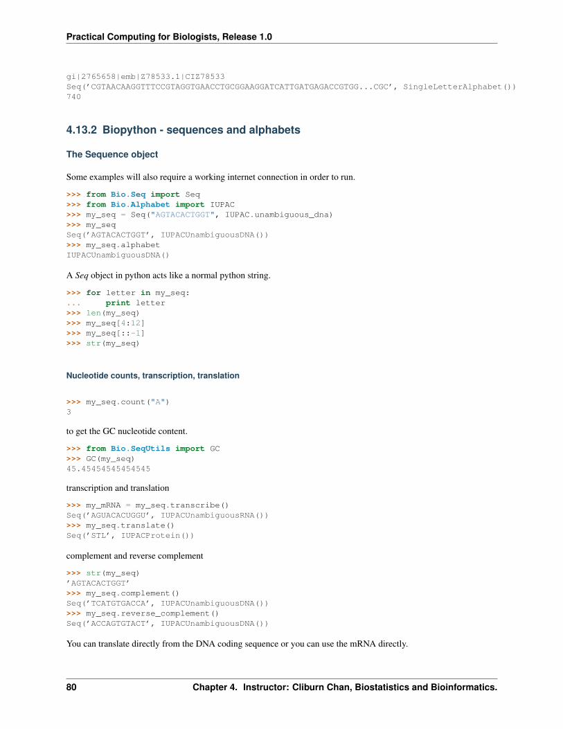
Practical Computing for Biologists, Release 1.0
gi|2765658|emb|Z78533.1|CIZ78533Seq(’CGTAACAAGGTTTCCGTAGGTGAACCTGCGGAAGGATCATTGATGAGACCGTGG...CGC’, SingleLetterAlphabet())740
4.13.2 Biopython - sequences and alphabets
The Sequence object
Some examples will also require a working internet connection in order to run.
>>> from Bio.Seq import Seq>>> from Bio.Alphabet import IUPAC>>> my_seq = Seq("AGTACACTGGT", IUPAC.unambiguous_dna)>>> my_seqSeq(’AGTACACTGGT’, IUPACUnambiguousDNA())>>> my_seq.alphabetIUPACUnambiguousDNA()
A Seq object in python acts like a normal python string.
>>> for letter in my_seq:... print letter>>> len(my_seq)>>> my_seq[4:12]>>> my_seq[::-1]>>> str(my_seq)
Nucleotide counts, transcription, translation
>>> my_seq.count("A")3
to get the GC nucleotide content.
>>> from Bio.SeqUtils import GC>>> GC(my_seq)45.45454545454545
transcription and translation
>>> my_mRNA = my_seq.transcribe()Seq(’AGUACACUGGU’, IUPACUnambiguousRNA())>>> my_seq.translate()Seq(’STL’, IUPACProtein())
complement and reverse complement
>>> str(my_seq)’AGTACACTGGT’>>> my_seq.complement()Seq(’TCATGTGACCA’, IUPACUnambiguousDNA())>>> my_seq.reverse_complement()Seq(’ACCAGTGTACT’, IUPACUnambiguousDNA())
You can translate directly from the DNA coding sequence or you can use the mRNA directly.
80 Chapter 4. Instructor: Cliburn Chan, Biostatistics and Bioinformatics.
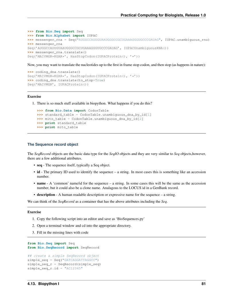
Practical Computing for Biologists, Release 1.0
>>> from Bio.Seq import Seq>>> from Bio.Alphabet import IUPAC>>> messenger_rna = Seq("AUGGCCAUUGUAAUGGGCCGCUGAAAGGGUGCCCGAUAG", IUPAC.unambiguous_rna)>>> messenger_rnaSeq(’AUGGCCAUUGUAAUGGGCCGCUGAAAGGGUGCCCGAUAG’, IUPACUnambiguousRNA())>>> messenger_rna.translate()Seq(’MAIVMGR*KGAR*’, HasStopCodon(IUPACProtein(), ’*’))
Now, you may want to translate the nucleotides up to the first in frame stop codon, and then stop (as happens in nature):
>>> coding_dna.translate()Seq(’MAIVMGR*KGAR*’, HasStopCodon(IUPACProtein(), ’*’))>>> coding_dna.translate(to_stop=True)Seq(’MAIVMGR’, IUPACProtein())
Exercise
1. There is so much stuff available in biopython. What happens if you do this?
>>> from Bio.Data import CodonTable>>> standard_table = CodonTable.unambiguous_dna_by_id[1]>>> mito_table = CodonTable.unambiguous_dna_by_id[2]>>> print standard_table>>> print mito_table
The Sequence record object
The SeqRecord objects are the basic data type for the SeqIO objects and they are very similar to Seq objects,however,there are a few additional attributes.
• seq - The sequence itself, typically a Seq object.
• id - The primary ID used to identify the sequence – a string. In most cases this is something like an accessionnumber.
• name - A ‘common’ name/id for the sequence – a string. In some cases this will be the same as the accessionnumber, but it could also be a clone name. Analagous to the LOCUS id in a GenBank record.
• description - A human readable description or expressive name for the sequence – a string.
We can think of the SeqRecord as a container that has the above attributes including the Seq.
Exercise
1. Copy the following script into an editor and save as ‘BioSequences.py’
2. Open a terminal window and cd into the appropriate directory.
3. Fill in the missing lines with code
from Bio.Seq import Seqfrom Bio.SeqRecord import SeqRecord
## create a simple SeqRecord objectsimple_seq = Seq("GATCAGGATTAGGCC")simple_seq_r = SeqRecord(simple_seq)simple_seq_r.id = "AC12345"
4.13. Biopython I 81

Practical Computing for Biologists, Release 1.0
simple_seq_r.description = "I am not a real sequence"
## print summaryprint simple_seq_r.idprint simple_seq_r.descriptionprint str(simple_seq_r.seq)print simple_seq_r.seq.alphabet
## translate the sequencetranslated_seq = simple_seq_r.seq.translate()print translated_seq
# exercise 1 -- translate the sequence only until the stop codon
# exercise 2 -- get the reverse complement of the sequence
# exercise 3 -- get the reverse of the sequence (just like for lists)
# exercise 4 -- get the GC nucleotide content
The Sequence IO object
There is one more object that we have to discuss and this the SeqIO object is like a container for multiple SeqRecordobjects.
import osfrom Bio import SeqIO
’’’We use a list here to save the gene records from a FASTA fileIf you have many records a dictionary will make the program faster.
’’’
## save the sequence records to a listallSeqRecords = []allSeqIDs = []pathToFile = os.path.join("..","data","ls_orchid.fasta")for seq_record in SeqIO.parse(pathToFile, "fasta"):
allSeqRecords.append(seq_record)allSeqIDs.append(seq_record.id.split("|")[1])print seq_record.idprint str(seq_record.seq)print len(seq_record)
## print out fun stuff about the sequencesprint "We found ", len(allSeqIDs), "sequences"print "information on the third sequence:"ind = 2seqRec = allSeqRecords[ind]print "\t", "GI number ", allSeqIDs[ind]print "\t", "full id ", seqRec.idprint "\t", "num nucleo. ", len(seqRec.seq)print "\t", "1st 10 nucleo.", seqRec.seq[:10]
82 Chapter 4. Instructor: Cliburn Chan, Biostatistics and Bioinformatics.

Practical Computing for Biologists, Release 1.0
Just as easy as it is to read a set of files we can save modified versions (i.e. QA). Also, it is almost the exact same codeas above to parse sequences from a GenBank (.gb) file.
There is really way to much to cover in the time we have, but if you have Next Generation Sequencing data then referto sections 4.8, 16.1.7 and 16.1.8 of the biopython tutorial. There is even support for binary formats (i.e. SFF).
4.13.3 Bibliographic notes
3. Cock, P J A and Antao, Tiago and Chang, J T and Chapman, B A and Cox, C J and Dalke, A and Friedberg, Iand Hamelryck, T and Kauff, F and Wilczynski B and de Hoon, M J L, Biopython: freely available Python toolsfor computational molecular biology and bioinformatics, Bioinformatics, Jun, 2009, 25, 11, 1422-3. PubMed.
4.14 Biopython II
4.14.1 Biopython - Entrez databases
NCBI’s Guidelines
Taken from the tutorial.
Before using Biopython to access the NCBI’s online resources (via Bio.Entrez or some of the other modules), pleaseread the NCBI’s Entrez User Requirements. If the NCBI finds you are abusing their systems, they can and will banyour access!
To paraphrase: For any series of more than 100 requests, do this at weekends or outside USA peak times. This isup to you to obey. Use the http://eutils.ncbi.nlm.nih.gov address, not the standard NCBI Web address. Biopythonuses this web address. Make no more than three requests every seconds (relaxed from at most one request every threeseconds in early 2009). This is automatically enforced by Biopython. Use the optional email parameter so the NCBIcan contact you if there is a problem. You can either explicitly set this as a parameter with each call to Entrez (e.g.include email=”[email protected]” in the argument list), or as of Biopython 1.48, you can set a global emailaddress:
>>> from Bio import Entrez>>> Entrez.email = "[email protected]"
Bio.Entrez will then use this email address with each call to Entrez. The example.com address is a reserved domainname specifically for documentation (RFC 2606). Please DO NOT use a random email – it’s better not to give anemail at all. The email parameter will be mandatory from June 1, 2010. In case of excessive usage, NCBI will attemptto contact a user at the e-mail address provided prior to blocking access to the E-utilities.
If you are using Biopython within some larger software suite, use the tool parameter to specify this. You can eitherexplicitly set the tool name as a parameter with each call to Entrez (e.g. include tool=”MyLocalScript” in the argumentlist), or as of Biopython 1.54, you can set a global tool name:
>>> from Bio import Entrez>>> Entrez.tool = "MyLocalScript"
The tool parameter will default to Biopython. For large queries, the NCBI also recommend using their session historyfeature (the WebEnv session cookie string, see Section 8.15). This is only slightly more complicated.
4.14. Biopython II 83
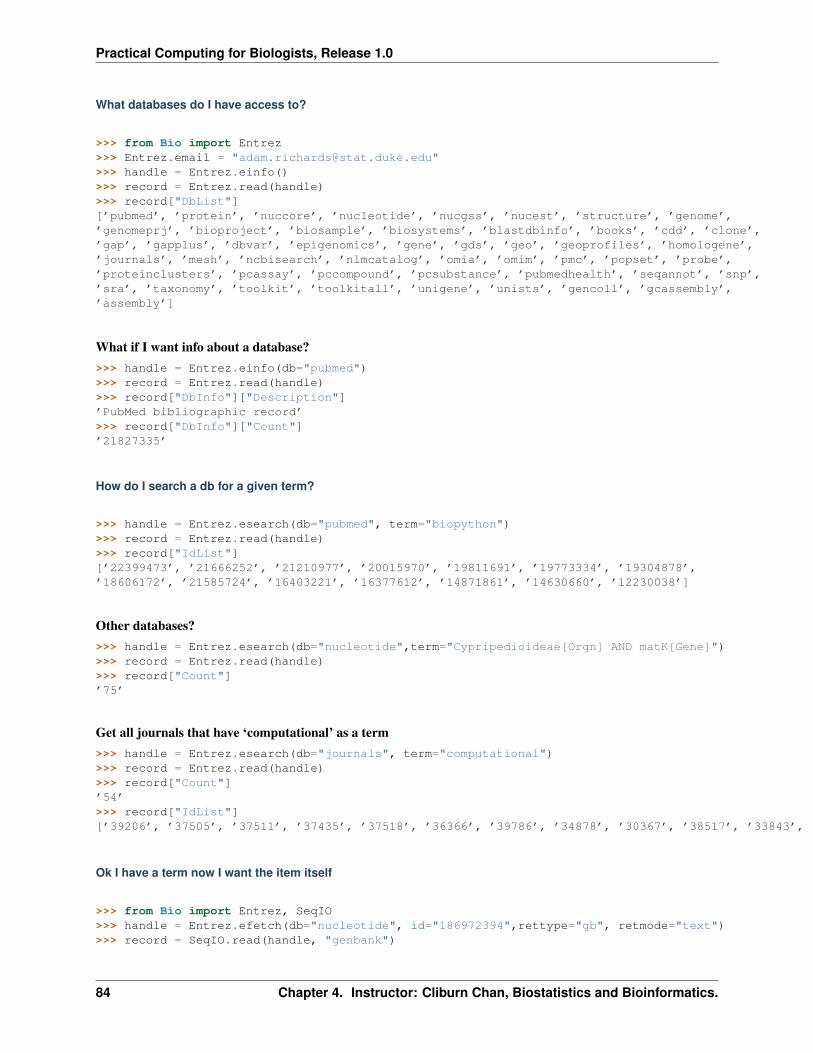
Practical Computing for Biologists, Release 1.0
What databases do I have access to?
>>> from Bio import Entrez>>> Entrez.email = "[email protected]">>> handle = Entrez.einfo()>>> record = Entrez.read(handle)>>> record["DbList"][’pubmed’, ’protein’, ’nuccore’, ’nucleotide’, ’nucgss’, ’nucest’, ’structure’, ’genome’,’genomeprj’, ’bioproject’, ’biosample’, ’biosystems’, ’blastdbinfo’, ’books’, ’cdd’, ’clone’,’gap’, ’gapplus’, ’dbvar’, ’epigenomics’, ’gene’, ’gds’, ’geo’, ’geoprofiles’, ’homologene’,’journals’, ’mesh’, ’ncbisearch’, ’nlmcatalog’, ’omia’, ’omim’, ’pmc’, ’popset’, ’probe’,’proteinclusters’, ’pcassay’, ’pccompound’, ’pcsubstance’, ’pubmedhealth’, ’seqannot’, ’snp’,’sra’, ’taxonomy’, ’toolkit’, ’toolkitall’, ’unigene’, ’unists’, ’gencoll’, ’gcassembly’,’assembly’]
What if I want info about a database?>>> handle = Entrez.einfo(db="pubmed")>>> record = Entrez.read(handle)>>> record["DbInfo"]["Description"]’PubMed bibliographic record’>>> record["DbInfo"]["Count"]’21827335’
How do I search a db for a given term?
>>> handle = Entrez.esearch(db="pubmed", term="biopython")>>> record = Entrez.read(handle)>>> record["IdList"][’22399473’, ’21666252’, ’21210977’, ’20015970’, ’19811691’, ’19773334’, ’19304878’,’18606172’, ’21585724’, ’16403221’, ’16377612’, ’14871861’, ’14630660’, ’12230038’]
Other databases?>>> handle = Entrez.esearch(db="nucleotide",term="Cypripedioideae[Orgn] AND matK[Gene]")>>> record = Entrez.read(handle)>>> record["Count"]’75’
Get all journals that have ‘computational’ as a term>>> handle = Entrez.esearch(db="journals", term="computational")>>> record = Entrez.read(handle)>>> record["Count"]’54’>>> record["IdList"][’39206’, ’37505’, ’37511’, ’37435’, ’37518’, ’36366’, ’39786’, ’34878’, ’30367’, ’38517’, ’33843’, ’37406’, ’40084’, ’36622’, ’39212’, ’33823’, ’32989’, ’33190’, ’38518’, ’40055’]
Ok I have a term now I want the item itself
>>> from Bio import Entrez, SeqIO>>> handle = Entrez.efetch(db="nucleotide", id="186972394",rettype="gb", retmode="text")>>> record = SeqIO.read(handle, "genbank")
84 Chapter 4. Instructor: Cliburn Chan, Biostatistics and Bioinformatics.
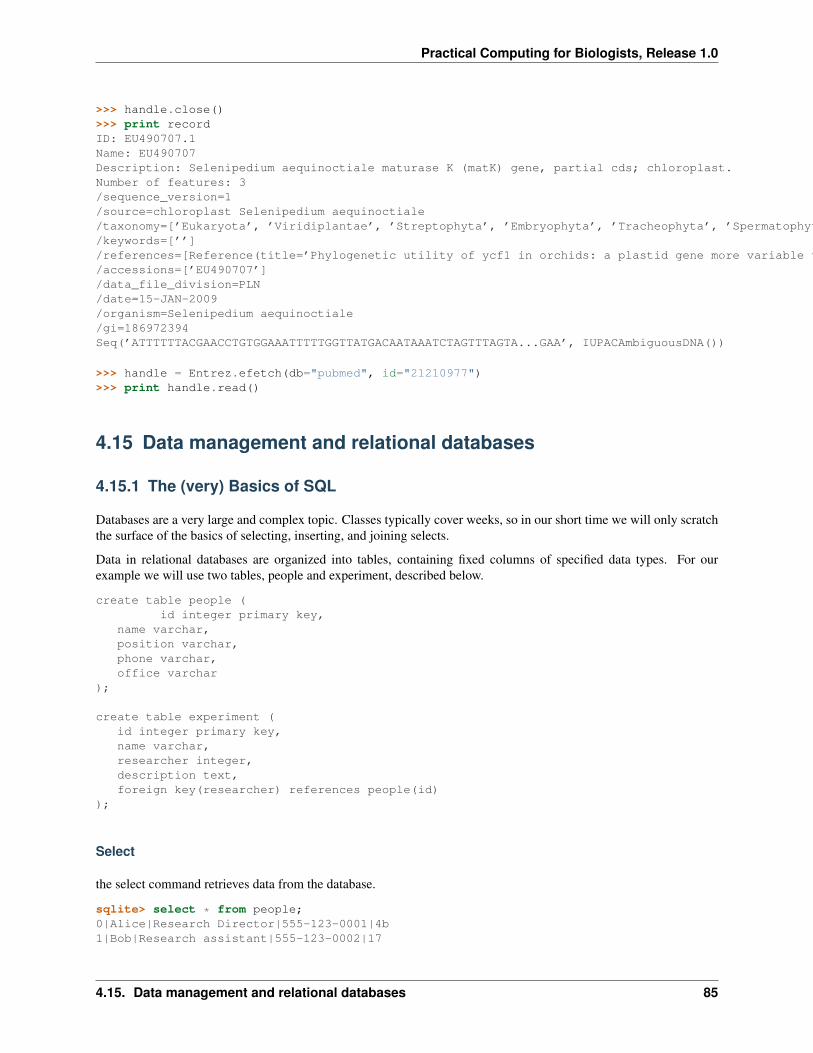
Practical Computing for Biologists, Release 1.0
>>> handle.close()>>> print recordID: EU490707.1Name: EU490707Description: Selenipedium aequinoctiale maturase K (matK) gene, partial cds; chloroplast.Number of features: 3/sequence_version=1/source=chloroplast Selenipedium aequinoctiale/taxonomy=[’Eukaryota’, ’Viridiplantae’, ’Streptophyta’, ’Embryophyta’, ’Tracheophyta’, ’Spermatophyta’, ’Magnoliophyta’, ’Liliopsida’, ’Asparagales’, ’Orchidaceae’, ’Cypripedioideae’, ’Selenipedium’]/keywords=[’’]/references=[Reference(title=’Phylogenetic utility of ycf1 in orchids: a plastid gene more variable than matK’, ...), Reference(title=’Direct Submission’, ...)]/accessions=[’EU490707’]/data_file_division=PLN/date=15-JAN-2009/organism=Selenipedium aequinoctiale/gi=186972394Seq(’ATTTTTTACGAACCTGTGGAAATTTTTGGTTATGACAATAAATCTAGTTTAGTA...GAA’, IUPACAmbiguousDNA())
>>> handle = Entrez.efetch(db="pubmed", id="21210977")>>> print handle.read()
4.15 Data management and relational databases
4.15.1 The (very) Basics of SQL
Databases are a very large and complex topic. Classes typically cover weeks, so in our short time we will only scratchthe surface of the basics of selecting, inserting, and joining selects.
Data in relational databases are organized into tables, containing fixed columns of specified data types. For ourexample we will use two tables, people and experiment, described below.
create table people (id integer primary key,
name varchar,position varchar,phone varchar,office varchar
);
create table experiment (id integer primary key,name varchar,researcher integer,description text,foreign key(researcher) references people(id)
);
Select
the select command retrieves data from the database.
sqlite> select * from people;0|Alice|Research Director|555-123-0001|4b1|Bob|Research assistant|555-123-0002|17
4.15. Data management and relational databases 85

Practical Computing for Biologists, Release 1.0
2|Charles|Research assistant|555-123-0001|243|David|Research assistant|555-123-0001|8
sqlite> select * from experiment;0|EBV Vaccine trial|0|A vaccine trial1|Flu antibody study|2|Study of the morphology of flu antibodies
The * in the select statement says to select all columns. If you only need a few of the columns you can select them byname.
sqlite> select name, phone from people;Alice|555-123-0001Bob|555-123-0002Charles|555-123-0001David|555-123-0001
sqlite> select name, description from experiment;EBV Vaccine trial|A vaccine trialFlu antibody study|Study of the morphology of flu antibodies
You can also limit the returned results to rows that match specified information using the where directive.
sqlite> select * from people where name == ’Alice’;0|Alice|Research Director|555-123-0001|4b
sqlite> select position from people where name == ’David’;Research assistant
Insert
Adding values to the database is done by using the insert statement.
sqlite> insert into people values ( Null, ’Edward’, ’Toadie’, ’None’, ’Basement’);sqlite> select * from people where name == ’Edward’;4|Edward|Toadie|None|Basement
Update
You can also change existing rows once they’ve been inserted. update takes a table name as it’s first argument followedby set column = value. With out a where clause this will set all row’s values. You there for will almost always use thewhere clause so that you get specific row/rows values updated.
sqlite> select * from people;0|Alice|Research Director|555-123-0001|4b1|Bob|Research assistant|555-123-0002|172|Charles|Research assistant|555-123-0001|243|David|Research assistant|555-123-0001|84|Edward|Toadie|None|Basementsqlite> update people set name=’Eddie’ where id=4;sqlite> select * from people;0|Alice|Research Director|555-123-0001|4b1|Bob|Research assistant|555-123-0002|172|Charles|Research assistant|555-123-0001|243|David|Research assistant|555-123-0001|84|Eddie|Toadie|None|Basement
86 Chapter 4. Instructor: Cliburn Chan, Biostatistics and Bioinformatics.

Practical Computing for Biologists, Release 1.0
Delete
Similar to updating you can delete rows from the database. The argument again will most likely want a where clauseto prevent deleting all rows in a table.
sqlite> select * from people;0|Alice|Research Director|555-123-0001|4b1|Bob|Research assistant|555-123-0002|172|Charles|Research assistant|555-123-0001|243|David|Research assistant|555-123-0001|84|Eddie|Toadie|None|Basementsqlite> delete from people where name=’Eddie’;sqlite> select * from people;0|Alice|Research Director|555-123-0001|4b1|Bob|Research assistant|555-123-0002|172|Charles|Research assistant|555-123-0001|243|David|Research assistant|555-123-0001|8
Joins
The power of relational databases lies in recording relations (the foreign key in the table declaration). To join twotables you use the join keyword in the select statement and provide a relation to join the two tables. Note, that sinceboth the people and experiment tables have a column called name we must cast the tables using the as statement.
sqlite> select p.name, e.name from people as p join experiment as e where e.researcher == p.id;Alice|EPV Vaccine trialCharles|Flu antibody study
4.15.2 Python and DBI
Working with relational databases is fairly simple with python,
1. Create a connection object
2. Execute a SQL statement
3. Iterate over results
In [1]: import sqlite3
In [2]: con = sqlite3.connect(’pcfb.sqlite’)
In [3]: r = con.execute(’select * from people’)
In [4]: for i in r:...: print i
(0, u’Alice’, u’Research Director’, u’555-123-0001’, u’4b’)(1, u’Bob’, u’Research assistant’, u’555-123-0002’, u’17’)(2, u’Charles’, u’Research assistant’, u’555-123-0001’, u’24’)(3, u’David’, u’Research assistant’, u’555-123-0001’, u’8’)(4, u’Edward’, u’Toadie’, u’None’, u’Basement’)
In [5]: r = con.execute(’select p.name, e.name from people as p join experiment as e where e.researcher == p.id’)
In [6]: for i in r:...: print ’Name: %s\n\tExperiment: %s’ % (i[0],i[1])
4.15. Data management and relational databases 87

Practical Computing for Biologists, Release 1.0
...:Name: Alice
Experiment: EPV Vaccine trialName: Charles
Experiment: Flu antibody study
4.15.3 Exercise:
Write a script to a add a new user and experiment to the database, remove Alice, and reassign her experiments to thenew user. Then have it print out all the experiment names with who owns each experiment.
4.16 Data analysis with Python
We have seen how to perform data munging with regular expressions and Python. For a refresher, here is a Pythonprogram using regular expressions to munge the Ch3observations.txt file that we did on day 1 using Tex-tWrangler.
import re
find = r’(\d+)\s+(\w{3})[\w\,\.]*\s+(\d+)\sat\s(\d+):(\d+)\s+([-\d\.]+)\s+([-\d\.]+).*’replace = r’\3\t\2.\t\1\t\4\t\5\t\6\t\7’
for line in open(’examples/Ch3observations.txt’):newline = re.sub(find, replace, line)print newline,
which when run produces this output
eris:pcfb cliburn$ python examples/regex.py1752 Jan. 13 13 53 -1.414 5.7811961 Mar. 17 03 46 14 3.62002 Oct. 1 18 22 36.51 -3.42211863 Jul. 20 12 02 1.74 133
This session will introduce you to the next stage of data analysis and data visualization. Because it is impossible to doany justice to these areas in a few hours, the aim of this session is to provide a taste of what analysis and visualizationin Python look like, and a tour of some of the many modules available for scientific computation in Python.
4.16.1 Curve Fitting
One common analysis task performed by biologists is curve fitting. For example, we may want to fit a 4 parameterlogistic (4PL) equation to ELISA data. The usual formula for the 4PL model is
f(x) =A−D
1 + (x/C)B+D
where x is the concentration, A is the minimum asymptote, B is the steepness, C is the inflection point and D is themaximum asymptote.
import numpy as npimport numpy.random as nprimport matplotlib.pyplot as pltfrom scipy.optimize import leastsq
88 Chapter 4. Instructor: Cliburn Chan, Biostatistics and Bioinformatics.

Practical Computing for Biologists, Release 1.0
def logistic4(x, A, B, C, D):"""4PL lgoistic equation."""return ((A-D)/(1.0+((x/C)**B))) + D
def residuals(p, y, x):"""Deviations of data from fitted 4PL curve"""A,B,C,D = perr = y-logistic4(x, A, B, C, D)return err
def peval(x, p):"""Evaluated value at x with current parameters."""A,B,C,D = preturn logistic4(x, A, B, C, D)
# Make up some data for fitting and add noise# In practice, y_meas would be read in from a filex = np.linspace(0,20,20)A,B,C,D = 0.5,2.5,8,7.3y_true = logistic4(x, A, B, C, D)y_meas = y_true + 0.2*npr.randn(len(x))
# Initial guess for parametersp0 = [0, 1, 1, 1]
# Fit equation using least squares optimizationplsq = leastsq(residuals, p0, args=(y_meas, x))
# Plot resultsplt.plot(x,peval(x,plsq[0]),x,y_meas,’o’,x,y_true)plt.title(’Least-squares 4PL fit to noisy data’)plt.legend([’Fit’, ’Noisy’, ’True’], loc=’upper left’)for i, (param, actual, est) in enumerate(zip(’ABCD’, [A,B,C,D], plsq[0])):
plt.text(10, 3-i*0.5, ’%s = %.2f, est(%s) = %.2f’ % (param, actual, param, est))plt.savefig(’logistic.png’)
4.16. Data analysis with Python 89

Practical Computing for Biologists, Release 1.0
It will be straightforward to modify this code to use, for example, a five parameter logistic or other equation, offeringa flexibility rarely available with standard analysis software.
4.16.2 Simulation-based statistics
With increasing computational power, it is now feasible to run many, many simulations to estimate parameters insteadof, or in addition to, the traditiional parameteric statistial methods. Most of these methods are based on some form ofresampling of the data available to estimate the null distribution, with well known examples being the bootstrap andpermuation resampling.
Before we do this, we need to understand a little about how to get random numbers. The numpy.random module hasrandom number generators for a variety of common probabiltiy distributions. These numbers are then used to simulatethe generation of new random samples. If the samples are chosen in a certain way, the statistics of the randomly drawnsamples can provide useful information about the properties of our original data sample. Here are some examples ofrandom number generation in iptyhon.
In [1]: import numpy.random as npr
In [2]: npr.random(5)Out[2]: array([ 0.93946009, 0.47060219, 0.10922504, 0.70776782, 0.41784061])
In [3]: npr.random((3,4))Out[3]:array([[ 0.29302404, 0.9372624 , 0.36149538, 0.59367473],
[ 0.42932372, 0.20717542, 0.18447385, 0.91159639],[ 0.83125219, 0.85109042, 0.32720074, 0.33453366]])
In [4]: npr.normal(5, 1, 4)Out[4]: array([ 3.45966714, 3.99815107, 5.0191997 , 5.93739408])
In [5]: npr.randint(1, 7, 10)Out[5]: array([6, 4, 1, 5, 6, 6, 1, 3, 4, 2])
90 Chapter 4. Instructor: Cliburn Chan, Biostatistics and Bioinformatics.

Practical Computing for Biologists, Release 1.0
In [6]: npr.uniform(1, 7, 10)Out[6]:array([ 3.55239006, 5.45862348, 1.77176392, 5.91184323, 2.49197674,
6.23527185, 2.51701757, 3.96170981, 6.43878462, 4.57074553])
In [7]: npr.binomial(n=10, p=0.2, size=(4,4))Out[7]:array([[5, 0, 4, 2],
[1, 1, 0, 2],[3, 2, 0, 2],[0, 1, 2, 4]])
In [8]: x = [1,2,3,4,5,6]
In [9]: npr.shuffle(x)
In [10]: xOut[10]: [2, 1, 5, 6, 4, 3]
In [11]: npr.permutation(10)Out[11]: array([2, 7, 4, 1, 6, 5, 8, 9, 3, 0])
For example, choosing a new sample with replacement from an existing sample (i.e. we draw one item from the data,record what it is, then replace it in the data and repeat to get a new sample) can be done efficiently in this way:
In [1]: import numpy as np
In [2]: import numpy.random as npr
In [3]: data = np.array([’tom’, ’jerry’, ’mickey’, ’minnie’, ’pocahontas’])
In [4]: idx = npr.randint(0, len(data), (4,len(data)))
In [5]: idxOut[5]:
array([[3, 0, 2, 1, 0],[4, 2, 3, 4, 4],[4, 0, 0, 0, 3],[2, 2, 3, 1, 4]])
In [6]: samples_with_replacement = data[idx]
In [7]: samples_with_replacementOut[7]:
array([[’minnie’, ’tom’, ’mickey’, ’jerry’, ’tom’],[’pocahontas’, ’mickey’, ’minnie’, ’pocahontas’, ’pocahontas’],[’pocahontas’, ’tom’, ’tom’, ’tom’, ’minnie’],[’mickey’, ’mickey’, ’minnie’, ’jerry’, ’pocahontas’]],
dtype=’|S10’)
In the next version of numpy (1.7.0), a new function choice is available in numpy.random to do the same thingwith a nicer syntax. Version 1.7.0 is only currently available from the git repository as source code that you mustcompile yourself, but should be available for easy_install/pip installation soon.
In [1]: import numpy.random as npr
In [2]: data = [’tom’, ’jerry’, ’mickey’, ’minnie’, ’pocahontas’]
4.16. Data analysis with Python 91

Practical Computing for Biologists, Release 1.0
# only availlable if you install numpy 1.7.0 from the git repositoryIn [3]: npr.choice(data, size=(4, len(data)), replace=True)---------------------------------------------------------------------------AttributeError Traceback (most recent call last)/Volumes/HD3/hg/pcfb/<ipython-input-3-84e7d179a607> in <module>()----> 1 npr.choice(data, size=(4, len(data)), replace=True)
AttributeError: ’module’ object has no attribute ’choice’
Moving on our first simulation example - if we want to plot the 95% confidence interval for the mean of our datasamples, we can use the bootstrap to do so. The basic idea is simple - draw many, many samples with replacementfrom the data available, estimate the mean from each sample, then rank order the means to estimate the 2.5 and 97.5percentile values for 95% confidence interval. Unlike using normal assumptions to calculate 95% CI, the resultsgenerated by the bootstrap are robust even if the underlying data are very far from normal.
import numpy as npimport numpy.random as nprimport pylab
def bootstrap(data, num_samples, statistic, alpha):"""Returns bootstrap estimate of 100.0*(1-alpha) CI for statistic."""n = len(data)idx = npr.randint(0, n, (num_samples, n))samples = x[idx]stat = np.sort(statistic(samples, 1))return (stat[int((alpha/2.0)*num_samples)],
stat[int((1-alpha/2.0)*num_samples)])
if __name__ == ’__main__’:# data of interest is bimodal and obviously not normalx = np.concatenate([npr.normal(3, 1, 100), npr.normal(6, 2, 200)])
# find mean 95% CI and 100,000 bootstrap sampleslow, high = bootstrap(x, 100000, np.mean, 0.05)
# make plotspylab.figure(figsize=(8,4))pylab.subplot(121)pylab.hist(x, 50, histtype=’step’)pylab.title(’Historgram of data’)pylab.subplot(122)pylab.plot([-0.03,0.03], [np.mean(x), np.mean(x)], ’r’, linewidth=2)pylab.scatter(0.1*(npr.random(len(x))-0.5), x)pylab.plot([0.19,0.21], [low, low], ’r’, linewidth=2)pylab.plot([0.19,0.21], [high, high], ’r’, linewidth=2)pylab.plot([0.2,0.2], [low, high], ’r’, linewidth=2)pylab.xlim([-0.2, 0.3])pylab.title(’Bootstrap 95% CI for mean’)pylab.savefig(’examples/boostrap.png’)
92 Chapter 4. Instructor: Cliburn Chan, Biostatistics and Bioinformatics.

Practical Computing for Biologists, Release 1.0
Note that the bootstrap function is a higher order function, and will return the boostrap CI for any valid statisticalfunction, not just the mean. For example, to find the 95% CI for the standard deviation, we only need to changenp.mean to np.std in the arguments:
# find standard deviation 95% CI bootstrap sampleslow, high = bootstrap(x, 100000, np.std, 0.05)
The function is also highly optimized, and takes under 2 seconds to calculate the boostrap mean for a data sample ofsize 300 using 100,000 bootstrap samples on a 4 year old MacBook Pro with 2.4 GHz Intel Core 2 Duo processor.
Permutation-resampling is another form of simulation-based statistical calculation, and is often used to evaluate thep-value for the difference between two groups, under the null hypothesis that the groups are invariant under labelpermutation. For example, in a case-control study, it can be used to find the p-value that hypothesis that the mean ofthe case group is different from that of the control group, and we cannot use the t-test because the distributions arehighly skewed.
import numpy as npimport numpy.random as nprimport pylab
def permutation_resampling(case, control, num_samples, statistic):"""Returns p-value that statistic for case is differentfrom statistc for control."""
observed_diff = abs(statistic(case) - statistic(control))num_case = len(case)
combined = np.concatenate([case, control])diffs = []for i in range(num_samples):
xs = npr.permutation(combined)diff = np.mean(xs[:num_case]) - np.mean(xs[num_case:])diffs.append(diff)
pval = (np.sum(diffs > observed_diff) +np.sum(diffs < -observed_diff))/float(num_samples)
return pval, observed_diff, diffs
if __name__ == ’__main__’:# make up some datacase = [94, 38, 23, 197, 99, 16, 141]control = [52, 10, 40, 104, 51, 27, 146, 30, 46]
4.16. Data analysis with Python 93

Practical Computing for Biologists, Release 1.0
# find p-value by permutation resamplingpval, observed_diff, diffs = \
permutation_resampling(case, control, 10000, np.mean)
# make plotspylab.title(’Empirical null distribution for differences in mean’)pylab.hist(diffs, bins=100, histtype=’step’, normed=True)pylab.axvline(observed_diff, c=’red’, label=’diff’)pylab.axvline(-observed_diff, c=’green’, label=’-diff’)pylab.text(60, 0.01, ’p = %.3f’ % pval, fontsize=16)pylab.legend()pylab.savefig(’examples/permutation.png’)
4.16.3 Data visualization
Data visualization is important for exploratory data analysis as well as for communication of scientific results. Usingipython with the -- pylab option provides an interarctive environment that is ideal for exploratory data analysis.The classic Anscombe data set illustrates the importance of visualization when analysing data. The Anscombe dataset consists of 4 different sets of (x,y) values, with esentially identical values for the
1. mean of x
2. variance of x
3. mean of y
4. variance of y
5. correlation between x and y
6. linear regression intercept and slope
Plotting the actual data sets quickly shows that the data sets are not as similar as suggested by the summary stattstics!
94 Chapter 4. Instructor: Cliburn Chan, Biostatistics and Bioinformatics.

Practical Computing for Biologists, Release 1.0
import numpy as npimport pylab
xs = np.loadtxt(’anscombe.txt’)for i in range(4):
x = xs[:,i*2]y = xs[:,i*2+1]A = np.vstack([x, np.ones(len(x))]).Tm, c = np.linalg.lstsq(A, y)[0]
pylab.subplot(2,2,i+1)pylab.scatter(x, y)pylab.plot(x, m*x+c, ’r’)pylab.axis([2,20,0,14])
pylab.savefig(’anscombe.png’)
For communication of results, matplotlib offers a huge range of graphics. We have only scratched the surface ofwhat the package has to offer. The fastest way to get a custom graphic to communicate your results is to look at thethumbnails at http://matplotlib.sourceforge.net/gallery.html. If one of the graphics looks appropirate for your needs,just click on the thumbnail to get the source code. You should now know enough Python to customize the graphic toyour specific needs.
4.17 Vector graphics with Inkscape
4.17.1 Graphical concepts
A quote from the text (PCFB).
No longer can you submit a photo that looks right; it has to be a “CMYK image, with 300 DPI at printed dimension,saved as a TIFF with LZW compression”. The goal here is to introduce a software that can help with some of these
4.17. Vector graphics with Inkscape 95

Practical Computing for Biologists, Release 1.0
requirements. Please refer to Chapter 17 for further depth than we go into here on graphics.
Vector and pixel images are probably concepts most biologists are familiar with. Pixel images (bitmap, raster) are auniform grid of colored dots. In vector art a line can be defined by two endpoints. The vector representation has theadvantage of being often easier to store. Also, the amount of information for vector art stays the same no matter howlarge the plot and as you zoom in vector art stays the same.
File formats that store vector based images include: PDF, EPS, SVG and AI. File formats that store pixel-based imagesare JPEG, PNG, TIFF, BMP and PSD. PDF, EPS and AI can store embedded pixel information (hybrid images).
It is always possible to go from vector to pixel art, but it is not so easy to go the other way. Another advantage ofvector art is that pixel text is not easily retrieved by a machine.
Pixel art is everywhere (photos, machine output), however if we have to create a completely plot then there are anumber of reasons to do so using vector graphics. Vector art is covered in chapter 18 of the book.
4.17.2 Inkscape
Inkscape uses the SVG (Scalable Vector Graphics) format for its files. SVG is an open standard widely supported bygraphic software.
Inkscape basics
QuickRef
NumPy command NoteCtrl+arrow pan or scroll the canvasCtrl+B hides scrollbars“-” “+” “=” zoom zoom zoomCtrl+N create a new inkscape documentsCtrl+O opens an exisiting svg fileCtrl+S saves the current fileholding Alt restricts movement in the move modeholding Ctrl preserves the original height/width ratio during resizespace or F1 activates the selector“[” and “]” rotate an objectarrows move objectsAlt+< and Alt+> resize and object. “<” and “>” work tootom bombadilhold Shift + click selects multiple objects
Getting familiar
1. open a new inkscape document
2. select the square shape and create a square or rectangle by pressing the mouse button once on your canvasdragging the mouse a little then letting go of the mouse. (try the control squares and circle)
3. Hit the spacebar to go into move/resize mode (try holding Ctrl)
4. Click on the rectangle again to change into rotate/skew mode. (try holding Ctrl) (try ‘[’,’]’,’<’,’>’)
96 Chapter 4. Instructor: Cliburn Chan, Biostatistics and Bioinformatics.
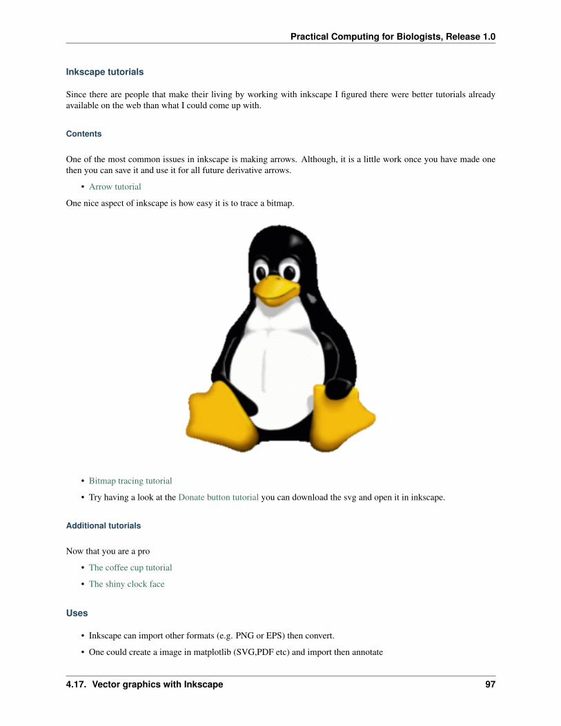
Practical Computing for Biologists, Release 1.0
Inkscape tutorials
Since there are people that make their living by working with inkscape I figured there were better tutorials alreadyavailable on the web than what I could come up with.
Contents
One of the most common issues in inkscape is making arrows. Although, it is a little work once you have made onethen you can save it and use it for all future derivative arrows.
• Arrow tutorial
One nice aspect of inkscape is how easy it is to trace a bitmap.
• Bitmap tracing tutorial
• Try having a look at the Donate button tutorial you can download the svg and open it in inkscape.
Additional tutorials
Now that you are a pro
• The coffee cup tutorial
• The shiny clock face
Uses
• Inkscape can import other formats (e.g. PNG or EPS) then convert.
• One could create a image in matplotlib (SVG,PDF etc) and import then annotate
4.17. Vector graphics with Inkscape 97

Practical Computing for Biologists, Release 1.0
• Resizing of images
• Adding text or shapes or colors to a bitmap
Additional Resources
• The inkscape documentation
• Nice set of tutorials
• Very nice gallery of wallpapers
• Python effects tutorial
4.18 Capstone Example
4.18.1 Analysing cytokine array data
In this final example, we will write a program to extract potentially useful summaries of data from a cytokine assaykindly donated by Herman Staats. You can download the file from the Data Samples page. As you can see, real worlddata analysis is far more messy than we have let on so far. Suppose we want to do two things - display the distributionof each cytokine on diffeerent days to see changes over time, and generate some QC summaries on what errors areassociated with what samples. Doing this manually in Excel will certainly be painful - what if Herman had stashedaway hundreds of such files and wanted to perform the analysis on every single one of them? A manual analysis mighttake weeks and will likely be ridden with errors as we grow increasingly bored and frustrated with the task.
So we will write a program to do this instead. The program will be quite challenging to write - we have broken thetask down into subtasks, and your job is to write functions to execute each subtask. Please ask for help if you get stuckat any point - we recognize that this will be an extemely challenging problem for most of you. OK - let’s begin ...
First, we need to convert the spreadsheet into a plain text format by exporting it within Excel. The Data Sam-ples page provides a tab delimited version exported from Excel; exporting to csv format is also fine if you pre-fer. (Note that Python modules to read and write Excel files are available - see http://www.python-excel.org/ andhttp://packages.python.org/openpyxl/ but as these were not covered in the workshop, we will continue to work withexported plain text files).
Notice that the data is arranged as a nice rectangular grid, with row 1 giving the header information, column 1 thesample names, and the rest the actual data values or various error messages. This suggests that we can use numpyarrays to manipulate the data, which will lead to a shorter program than the use of the csv module to parse every item.Notice also that there is a mixture of strings and numbers in the spreadsheet, and numpy only works with arrays ofall the same type. Since strings can represent numbers but not vice versa, we will first load the data as an array ofstrings using the numpy loadtxt function. Our strategy is then to manipulate the data so that apart from the header(row 1) and sample (column 1) information, everything else is converted to an array of floats for statistical analysisand visualization.
Our first task is to read the file and convert to an array of strings, which can be done with the loadtxt function. Wefirst see what loadtxt does:
In [4]: import numpy as np
In [5]: help(np.loadtxt);
98 Chapter 4. Instructor: Cliburn Chan, Biostatistics and Bioinformatics.

Practical Computing for Biologists, Release 1.0
4.18.2 Exercise
Write a function called read_table to load a tab delimited file as a numpy array using the numpy loadtxtfunction. The function should take a filename and an optional delimiter (e.g. ‘t’ for TDL and ‘,’ for CSV) as arguments,and return a numpy array of strings:
def read_table(filename, delimiter=’\t’):# your code goes here and should return a numpy array of strings
Now that we have the table as a numpy array, let’s focus on converting the middle “data” portion into an array offloats. We need to somehow convert all those error or warning messages into numbers. One simple way to do thiis isto encode each unique message as a number that cannot be mistaken for a data value. Since concentrations are nevernegative, we will use the negative integers to encode the errors. But in order to do the encoding, we first need to findout what types of messages exist in the data set.
4.18.3 Exercise
Write a function that finds all the warnings in the table returned by the previous read_table function and returns adictionary of {warning : code} where warning is a string (e.g. ‘Bead Issues’ or ‘UN’) and code is a negative number.Each unique warning should be given a different negative number. Basically we want to find all strings in the “data”part of the table, i.e. table[1:, 1:], and everytime we find a string, we shove it into the dictionary if it is not alreadythere with a new negative number code:
def parse_warnings(table):# your code goes here and should return a dictionary of warnings
Next, let’s deal with the sample information in column 1, excluding row 1, column 1. We notice that the same samplename can occur on multiple rows - let’s create a dictionary whose key is the sample name, and whose value is the rownumber minus one (minus one because we want row number = 0 to index the first data row, not the header information).
4.18.4 Exercise
Complete the function:
def parse_samples(table):# your code goes here and should return a dictionary of lists of row numbers for each sample
Parsing the header information is slightly more challenging. We notice that two different pieces of information areprovided by each cell in the header - the cytokine name (e.g. IL-2 beta) and the day the sample was taken (e.g. day 3).Each cytokine is sampled on multple days (0, 3 and 28). We want to create a dictionary that will tell us what columnwe can find the values for a given cytokine, day combination. One way to deal with the fact that the same cytokine issampled on multiple days is to use a dictionary of dictionaries. In particular, we will construct a dictionary whose keyis a cytokine name, and whose value is another dictionary. This other dictionary has a key representing the day, and avalue representing the column number minus one for the (cytokine, day) combination.
4.18.5 Exercise
Complete the function:
def parse_headers(table):# your code goes here and should return a dictionary of dictionaries as described in the text
We finally get to convert the data from an array of strings to an array of floats. Replace all the warning messages withthe code numbers, and return a new array of floats comprising the following subarray - table[1:, 1:].
4.18. Capstone Example 99

Practical Computing for Biologists, Release 1.0
4.18.6 Exercise
Complete the function:
def parse_data(table, warning_dict):# your code goes here and should return an array of floats containing values for the entries in table[1:, 1:]
Let’s consolidate all the above functions into a single function that when given a filename, reads the file and breaks itdown into a sample dictionary, a cytokine dicitonary and a data array. My function is shown below - you only have tochange the names to match the structures that you created:
def parse_cytokine_table(filename):# extract data and sample and cytokine mapping dictinaries from tabletable = read_table(filename)
warning_dict = parse_warnings(table)sample_mapper = parse_samples(table)cytokine_mapper = parse_headers(table)data = parse_data(table, warning_dict)return warning_dict, sample_mapper, cytokine_mapper, data
Well done! The most difficult part of the program is now complete. We next see how we can use the structures wehave created to make summaries of the data. First, let’s use a box-and-whiskers plot to show the distribution of eachcytokine over days 0, 3 and 28. Generate one such figure for each such cytokine - it should look something like this.
4.18.7 Exercise
Write the function to generate the box-and -whiskers plots. Remember that the negative numbers are not reallycytokine concentrations and should not be used for plotting:
def plot_cytokine(cytokine, cytokine_mapper, data, save=False, directory=’.’):# generate plots like the one shown
100 Chapter 4. Instructor: Cliburn Chan, Biostatistics and Bioinformatics.

Practical Computing for Biologists, Release 1.0
# if save is False, don’t save but simply show each figure# if save if True, save to disk with savefig(directory/filename)
Finally, let’s write the QC data to file. There seem to be an enormous number of errors in this file - let’s summarizethem so that Herman can figure out what is going on! Generate one text file per unique warning, where each row hastwo columns - the sample name, and the number of that type of warning associated with the sample. For instance, theBead_Issues.txt file will contain the following values:
0921-X-2-2 21059-X-2-2 120273-X-2-2 20740-X-2-2 40263-X-2-2 180175-X-2-2 20012-X-2-2 40108-X-2-2 10066-X-2-2 20057-X-2-2 120313-X-2-2 70103-X-2-2 250685-X-2-2 20799-X-2-2 40749-X-2-2 160693-X-2-2 11023-X-2-2 60300-X-2-2 2
Complete the function:
def write_qc(qc, directory=’.’):# write QC reports as described# save to the directory given and use the mesage name + ’.txt’ as the filename
That wraps up the coding part of this final capstone example.
4.18.8 Final Exercise
Now that you know how to think like a programmer, don’t create such spreadsheets in the future if possible! Designspreadsheets so that the information is “machine-friendly”. What are some of the ways you can make the originalspreadsheet more “machine-friendly” if you could change the design?
The full program that for parsing the cytokne assay file:
1 """Intermediate example of data munging using numpy.2 Task: Summarize the change in concentration over time for each cytokine.3 Input: An Excel worksheet exported as a tab delimited file4 Output: Figures summarizing concentrations of individual cytokines over time.5 """6
7 import numpy8 import pylab9 import os
10
11 def parse_cytokine_table(filename):12 # extract data and sample and cytokine mapping dictinaries from table13 table = read_table(filename)14
15 warning_dict = parse_warnings(table)
4.18. Capstone Example 101

Practical Computing for Biologists, Release 1.0
16 sample_mapper = parse_samples(table)17 cytokine_mapper = parse_headers(table)18 data = parse_data(table, warning_dict)19 return warning_dict, sample_mapper, cytokine_mapper, data20
21 def read_table(filename, delimiter=’\t’):22 # read data into an array of strings23 # this can also be done by standard data munging techniques24 # but would be more painful25 return numpy.loadtxt(filename, dtype=’string’, delimiter=delimiter)26
27 def parse_warnings(table):28 # create a dictionary to convert missing data codes into numeric codes29 data = table[1:, 1:]30 warning_dict = {}31 idx = -132 for x in data.ravel():33 try:34 float(x)35 except:36 if x not in warning_dict:37 warning_dict[x] = idx38 idx -= 139 return warning_dict40
41 def parse_samples(table):42 # create a dictionary that returns the rows where each sample has data43 samples = table[1:,0]44 sample_mapper = {}45 for i, sample in enumerate(samples):46 sample_mapper.setdefault(sample, []).append(i)47 return sample_mapper48
49 def parse_headers(table):50 # get header information in first row51 headers = table[0,:]52 # parse header informtion to find columns for each cytokine/day combination53 cytokine_mapper = {}54 for i, label in enumerate(headers[1:]):55 cytokine, day = label.split(’day’)56 cytokine_mapper.setdefault(cytokine.strip(), {})[int(day)] = i57 return cytokine_mapper58
59 def parse_data(table, warning_dict):60 # convert missing data from strings to code numbers for analysis61 data = table[1:, 1:]62 for warning in warning_dict:63 data[data==warning] = warning_dict[warning]64 data = data.astype(’float’)65 return data66
67 def plot_cytokine(cytokine, cytokine_mapper, data, save=False, directory=’.’):68 # generate box and whiskers plot for distribution of a single cytokine69 idx_dict = cytokine_mapper[cytokine]70 xs = data[:, sorted(idx_dict.values())]71
72 # collect measured values for each day in a list ignoring missing values73 ys = []
102 Chapter 4. Instructor: Cliburn Chan, Biostatistics and Bioinformatics.
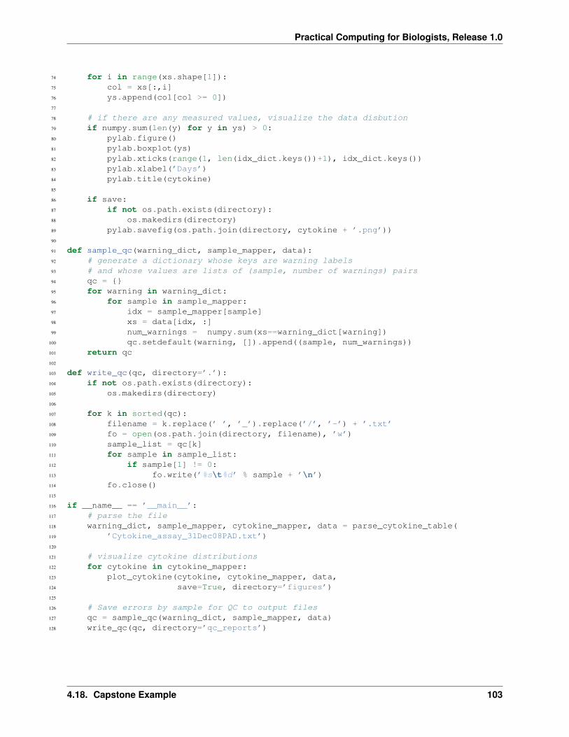
Practical Computing for Biologists, Release 1.0
74 for i in range(xs.shape[1]):75 col = xs[:,i]76 ys.append(col[col >= 0])77
78 # if there are any measured values, visualize the data disbution79 if numpy.sum(len(y) for y in ys) > 0:80 pylab.figure()81 pylab.boxplot(ys)82 pylab.xticks(range(1, len(idx_dict.keys())+1), idx_dict.keys())83 pylab.xlabel(’Days’)84 pylab.title(cytokine)85
86 if save:87 if not os.path.exists(directory):88 os.makedirs(directory)89 pylab.savefig(os.path.join(directory, cytokine + ’.png’))90
91 def sample_qc(warning_dict, sample_mapper, data):92 # generate a dictionary whose keys are warning labels93 # and whose values are lists of (sample, number of warnings) pairs94 qc = {}95 for warning in warning_dict:96 for sample in sample_mapper:97 idx = sample_mapper[sample]98 xs = data[idx, :]99 num_warnings = numpy.sum(xs==warning_dict[warning])
100 qc.setdefault(warning, []).append((sample, num_warnings))101 return qc102
103 def write_qc(qc, directory=’.’):104 if not os.path.exists(directory):105 os.makedirs(directory)106
107 for k in sorted(qc):108 filename = k.replace(’ ’, ’_’).replace(’/’, ’-’) + ’.txt’109 fo = open(os.path.join(directory, filename), ’w’)110 sample_list = qc[k]111 for sample in sample_list:112 if sample[1] != 0:113 fo.write(’%s\t%d’ % sample + ’\n’)114 fo.close()115
116 if __name__ == ’__main__’:117 # parse the file118 warning_dict, sample_mapper, cytokine_mapper, data = parse_cytokine_table(119 ’Cytokine_assay_31Dec08PAD.txt’)120
121 # visualize cytokine distributions122 for cytokine in cytokine_mapper:123 plot_cytokine(cytokine, cytokine_mapper, data,124 save=True, directory=’figures’)125
126 # Save errors by sample for QC to output files127 qc = sample_qc(warning_dict, sample_mapper, data)128 write_qc(qc, directory=’qc_reports’)
4.18. Capstone Example 103

Practical Computing for Biologists, Release 1.0
104 Chapter 4. Instructor: Cliburn Chan, Biostatistics and Bioinformatics.

INDEX
Aassignments, 9
Pparticipants, 11
Rreferences, 10
105