Consortium of Organizations for Strong-Motion Observation

Systems

COSMOS Annual Meeting Technical Session 2009

Summary

Practical Application of the New ASCE 7-10 Required Procedures for Determining Site Specific Ground

Motions

Jennie Watson-Lamprey

November 2010

COSMOS

1301 South 46th Street Richmond, CA 94804

1

Summary of COSMOS Annual Meeting Technical Session 2009

Practical Application of the New ASCE 7-10 Required Procedures for Determining Site Specific Ground Motions

Prepared for COSMOS

Jennie Watson-Lamprey

1 Introduction The 2009 COSMOS Annual Meeting/Technical Session focused on application of the new ASCE 7-10 site-specific ground-motion requirements. The ASCE 7-10 contains a number of ground-motion changes, including use of risk-targeted ground motion, a change in the definition of ground motion, and new methods for estimating deterministic ground motions, shown in Figure 1. Presentations were made during the Technical Session on these new procedures and some technical issues associated with the procedural changes were highlighted. The issues addressed included whether the change in the definition of ground motion is affecting the intended structural collapse probability, how the maximum rotated component should be calculated, and how to develop suites of two-component time histories.

Figure 1: C. Kircher. First presented at the EERI Seminar on Next Generation Attenuation Models (September 2009)

1

2 Key Technical Changes to Ground Motions 

2.1 Risk Targeted Ground Motions 

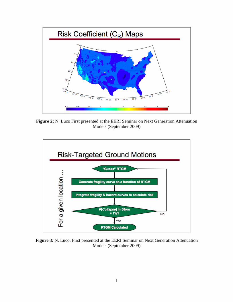
Probabilistic MCE ground motions have been defined as those having a 2% probability of being exceeding in 50 years. That is, they have a uniform hazard across all regions. Designing for uniform hazard ground motion does not result in uniform probability of collapse when differing seismic regions are combined. As Kircher (2009) pointed out and as was recognized in ATC 3-06 (1978), “it is really the probability of structural failure with resultant casualties that is the concern” for building codes. With this in mind, the new risk-targeted ground motions aim to have a uniform collapse risk objective of 1% in 50 years. There are two ways to calculate these new risk-targeted ground motions, as presented by Luco (2009). First, the uniform hazard ground motion can be calculated using the USGS seismic hazard maps and the Risk Coefficient shown in Figure 2 applied to the ground motion to generate the risk-targeted ground motion. These risk coefficients have been pre-determined for the user and are included in ASCE 7-10 and 2009 NEHRP. The risk coefficient is the ratio of the risk-targeted ground motion and the uniform hazard ground motion at a site. The risk-targeted ground motion is determined by initially guessing a ground motion consistent with the USGS site seismic hazard model, integrating that ground motion with a generic fragility curve, determining if the probability of collapse goal was achieve, and then adjusting the ground motion estimate if necessary. This procedure is repeated until the estimated risk-targeted ground motion produces the desired probability of collapse, as shown in Figure 3. The second method for calculating the risk-targeted ground motions is to follow the procedure outlined in Figure 3 using a site-specific hazard curve and fragility.

2.2 Direction of Ground Motion – Switch to Maximum Rotated Component 

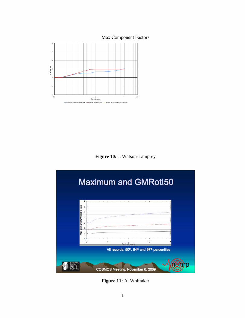
The definition of ground motion was changed to the maximum rotated component of ground motion, as shown in Figure 4. According to Kircher (2009), records applied along a single axis are approximately 20% less likely to collapse a structure as compared to a bi-axial application of the same records. In general, real structures can fail in any direction; thus, Kircher stated that the stronger component governs collapse and fails the structure in the direction of application. The definition of ground motion was changed to supply the largest component of ground motion. Near-fault ground motion ratios to convert geomean to maximum rotated component were presented by Whittaker (2009) and are shown in Figure 5. These ratios apply a factor of 1.1 for periods less than 1, and a factor of 1.3 for periods of 1 or greater.

1

Figure 2: N. Luco First presented at the EERI Seminar on Next Generation Attenuation Models (September 2009)

Figure 3: N. Luco. First presented at the EERI Seminar on Next Generation Attenuation Models (September 2009)

1

Figure 4: A. Whittaker

Figure 5: A. Whittaker

1

Figure 6: N. Luco. First presented at the EERI Seminar on Next Generation Attenuation Models (September 2009)

2.3 Near­Fault Deterministic Ground Motions 

Deterministic ground motions in ASCE 7-10 were presented by Luco (2009) and were calculated by obtaining the median ground motions from the USGS and then applying two factors, as shown in Figure 6. The first approximates the 84th percentile of ground motion by multiplying the spectrum by a factor of 1.8. The second converts the ground motion from geomean to the maximum rotated component by multiplying the spectrum the spectrum by a factor of 1.1 at short periods, and a factor of 1.3 at long periods, as presented by Whittaker (2009).

2.4 Site Response Analysis for Liquefaction 

The new seismic provisions in ASCE 7-10 for site-response analysis of liquefaction were presented by Crouse (2009). Ground-motion time series for three-dimensional dynamic analyses are no longer scaled to 1.3 times the target spectrum; instead, the square-root of the sum of the squares of the two time series are scaled to the target spectrum, as shown in Figure 7. The ground motion parameter used for the liquefaction analysis is the geomean peak ground acceleration instead of an estimate of the peak ground acceleration based on the spectral values. Crouse stated that the reason why this was done was the liquefaction evaluation procedures have been calibrated based on the geomean values. Separate PGA maps for liquefaction evaluations are provided in ASCE 7-10.

1

Figure 7: C. B. Crouse

3 Technical Issues Regarding Procedural Changes 

3.1 Issue 1:  Does switching to maximum rotated component from geomean bias the hazard levels intended for application? 

While Kircher (2009) implied that structures can fail in any direction and that the larger component of ground motion determines the direction of collapse, Stewart (2009) presented an alternative hypothesis. Stewart (2009) agreed that for structures that have similar behavior in multiple directions, such as flag poles and structures with a similar strength and stiffness in both directions, we can conceptualize that the maximum rotated component of ground motion controls collapse. He pointed out, however, that there is no research demonstrating this. In contrast, most structures have different behavior in their two principal axes. This is true of dams, bridges, and some buildings whose transverse and longitudinal axes have different periods. For these types of structures, Stewart (2009) suggested that the two directions are best analyzed separately, thus the arbitrary component of ground motion or the geomean ground motion is most appropriate. When the geomean ground motion is most appropriate, but the maximum rotated component of ground motion is used instead, the input ground motion is larger than it would be if the appropriate ground motion had been used. This is consistent with using a lower annual probability of exceedance for the ground motion, as demonstrated in Figure 8. Stewart (2009) went on to suggest that the lowering of the ground motion effected by the NGA on the USGS maps, as shown in Figure 9, was the impetus for the change in the definition of ground motion.

1

Figure 8: J. Stewart

Figure 9: J. Stewart

1

Bob Bachman asked Charlie Kircher whether the definition of ground motion was changed in response to the NGA. Charlie Kircher replied that is was “not a fair characterization of the committee’s efforts.” He implied that the lowering of the ground motion by the NGA instead allowed the committee to make a change that they thought was technically correct without having a large impact on design ground motion from one building code to the next. Bob Bachman then asked Nico Luco if the return period of ground motion was being increased by using the maximum rotated component of ground motion. Norm Abrahamson replied that the key issue here is that there be consistency between the fragility and the hazard curve. If the fragilities were calculated for a three-dimensional structure using the maximum rotated component of ground motion as the predictor of collapse, then everything is consistent and the probability of collapse is being estimated correctly. Nico Luco replied that the analyses were not three-dimensional. Charlie Kircher added that the analyses were two-dimensional and that most structures are actually analyzed as two-dimensional structural systems.

3.2 Issue 2:  How should the maximum rotated component spectrum be determined? 

3.2.1 Which factors should be used? Watson-Lamprey (2009) showed that there are a number of choices for converting to the maximum rotated component of ground motion, as shown in Figure 10. There is little difference between the Watson-Lamprey and Boore (2007) model and the Beyer and Bommer model, but the factors presented by Whittaker (2009) and used in ASCE 7-10 are lower in the short-period range, as shown in Figure 5. Norman Abrahamson posed the question of which factor to use to convert to the maximum rotated component, those in ASCE 7-10 or those of Watson-Lamprey and Boore [REF]. Andrew Whittaker replied that the factors came from different datasets and thus cannot be compared. Jennie Watson-Lamprey then pointed out that some of the average conversion factors from geomean to the maximum rotated component presented by Whittaker (2009) were less than one, demonstrating that the ASCE 7-10 factors make a change in the median values of the NGA close to the fault. Jennie Watson-Lamprey then asked if this change in the median values was intended. Andrew Whittaker replied that they had not intended to change the median value of the NGA relationships. Norm Abrahamson then replied that if that the was case, then the Watson-Lamprey and Boore [REF] factors should be used to calculate the maximum rotated component.

3.2.2 Should directivity effects be applied if the maximum rotated component is used? 

Gregor (2009) presented the effect of combining directivity effects with maximum rotated component ground motion on probabilistic seismic hazard analyses. He showed that for a site in San Francisco the ground motion with a 2% probability of exceedance in 50 years is increased 85% when both factors are included.

1

Max Component Factors

1

1.1

1.2

1.3

1.4

1.5

1.6

0.1 1 10

Max/GMRotI

Period (sec)

Watson-Lamprey and Boore Beyer and Bommer Huang et al. - Average Directivity

Figure 10: J. Watson-Lamprey

Figure 11: A. Whittaker

1

Figure 12: N. Gregor

Norm Abrahamson asked the panel whether the effects of directivity on the geomean should be combined with the factor to convert geomean to maximum rotated component ground motion. Andrew Whittaker replied that that would be the sensible way to perform a probabilistic seismic hazard analysis. Norm Abrahamson followed up by asking the panel if anyone saw an inconsistency with including directivity. There were no objections from the panel.

3.2.3 Issue 3:  How should two­component time histories be developed using the maximum rotated component? 

When developing two-component time histories, ASCE 7-10 states that the average of the square root of the sum of the squares spectra for all component pairs should not fall below the target spectrum, as shown in Figure 13. This method has already been adopted by OSHPD in the Code Application Notice CAN2-1802A.6.2. Walker (2009) pointed out that rapid-fire code changes of this sort can cost owners or consultants extra money. Golesorkhi (2009) presented the use of this method for a hospital project in San Francisco. He demonstrated that the scaled time histories, shown in Figure 14, had an average maximum rotated component spectrum that was less than the target spectrum. He pointed out that in his opinion there was no check in ASCE 7-10 to catch such a situation.

1

Figure 13: R. Golesorkhi

Figure 14: R. Golesorkhi

1

Figure 15: A. Bastani A healthcare facility project in Northern California used a similar scaling procedure to develop time histories, as presented by Bastani (2009). For this application, both components of ground motion were scaled to a spectrum defined by the maximum rotated component and divided by the square root of 2. The pairs were then rotated to find the maximum component and compared with the target spectrum. The average fell below the target and the matched ground motions were then scaled up to meet the target spectrum on average and not fall below 90% of the target. Norm Abrahamson pointed out to the panel that if the square root of the sum of the squares spectrum of a pair of time histories is scaled to match a target maximum rotated component spectrum, the maximum rotated component of the time history pair will be less than the target spectrum, as demonstrated by the two examples. Conversely, if the time histories are rotated to the strike normal and strike parallel components of ground motion and the strike normal component is scaled to match a target maximum rotated component spectrum, then the maximum rotated component of the time history pair will be greater than the target spectrum. Norm Abrahamson asked the panel what the intent of the scaling rule was. The consensus of those panelists involved with the process was that the intent was that the maximum rotated component of the scaled time histories should come up to the spectrum that defines it. Watson-Lamprey (2009) presented the results of an analysis using the NGA database that showed that for 92% of time history pairs, at all magnitudes and distances, a single component of ground motion can be found such that the spectrum of the rotated component at periods of 1, 2, and 4 seconds reaches 90% of the amplitude of the

1

maximum rotated component spectrum. This suggests a new procedure for developing suites of time history pairs. In this procedure a target spectrum is defined that is 90% of the target maximum rotated component spectrum. The selected time-history pairs are then rotated to a principal axis of ground motion and scaled to meet the 90% target spectrum. Norm Abrahamson asked the panel if time histories should be rotated to a principal axis before scaling. Charlie Kircher replied that this is the right idea: “I like it. I’m on board.”

4 References  Bastani, A. (2009), “Application of ASCE 7-05 and Recent OSHPD Express Terms for

Selection of Ground Motions for a Healthcare Facility”, COSMOS Annual Meeting Technical Session, November 6, 2009, Millbrae, CA.

Crouse, C.B. (2009), “New Liquefaction Requirements and Associated PGA Maps”,

COSMOS Annual Meeting Technical Session, November 6, 2009, Millbrae, CA. Golesorkhi, R. (2009), “Selection of Ground Motions for a Hospital Application”,

COSMOS Annual Meeting Technical Session, November 6, 2009, Millbrae, CA. Gregor, N. (2009), “ Application of Directivity and Maximum Rotated Component

Factors”, COSMOS Annual Meeting Technical Session, November 6, 2009, Millbrae, CA.

Kicher, C. (2009), “Basis for the New Risk-Targeted Ground Motion Maps”, COSMOS

Annual Meeting Technical Session, November 6, 2009, Millbrae, CA. Luco, N. (2009), “Preparation of New Seismic Design Maps and Associated Web

Products”, COSMOS Annual Meeting Technical Session, November 6, 2009, Millbrae, CA.

Stewart, J. (2009), “Should Design Spectra in Building Codes Be Specified from the

Maximum Component or the Average Horizontal? ”, COSMOS Annual Meeting Technical Session, November 6, 2009, Millbrae, CA.

Walker, M. (2009), “NGA in Practice: Implementation of NGA in Accordance with the

Codes”, COSMOS Annual Meeting Technical Session, November 6, 2009, Millbrae, CA.

Whittaker, A. (2009), “Maximum Direction Shaking: Amplitude and Orientation”,

COSMOS Annual Meeting Technical Session, November 6, 2009, Millbrae, CA.

1

Watson-Lampre, J. (2009), “Factors for Calculating Maximum Rotated Component”, COSMOS Annual Meeting Technical Session, November 6, 2009, Millbrae, CA.

Watson-Lamprey, J. and D.M. Boore (2007), "Beyond SaGMRotI, Conversion to SaArb,

SaSN and SaMaxRot", Bulletin of the Seismological Society of America, v. 97; no. 5; p. 1511-1524.