pp-wave reflection coefficients in weakly anisotropic

GEOPHYSICS, VOL. 63, NO. 6 (NOVEMBER-DECEMBER 1998); P. 2129–2141, 4 FIGS.

PP-wave reflection coefficients in weaklyanisotropic elastic media

Vaclav Vavrycuk∗ and Ivan Psencık∗

ABSTRACT

Approximate PP -wave reflection coefficients forweak contrast interfaces separating elastic, weakly trans-versely isotropic media have been derived recentlyby several authors. Application of these coefficients islimited because the axis of symmetry of transverselyisotropic media must be either perpendicular or paral-lel to the reflector. In this paper, we remove this lim-itation by deriving a formula for the PP -wave reflec-tion coefficient for weak contrast interfaces separatingtwo weakly but arbitrarily anisotropic media. The for-mula is obtained by applying the first-order perturba-tion theory. The approximate coefficient consists of asum of the PP -wave reflection coefficient for a weakcontrast interface separating two background isotropichalf-spaces and a perturbation attributable to the devia-tion of anisotropic half-spaces from their isotropic back-grounds. The coefficient depends linearly on differencesof weak anisotropy parameters across the interface. Thissimplifies studies of sensitivity of such coefficients to theparameters of the surrounding structure, which repre-sent a basic part of the amplitude-versus-offset (AVO)

or amplitude-versus-azimuth (AVA) analysis. The reflec-tion coefficient is reciprocal. In the same way, the for-mula for the PP -wave transmission coefficient can bederived. The generalization of the procedure presentedfor the derivation of coefficients of converted waves isalso possible although slightly more complicated. De-pendence of the reflection coefficient on the angle ofincidence is expressed in terms of three factors, as inisotropic media. The first factor alone describes normalincidence reflection. The second yields the low-order an-gular variations. All three factors describe the coefficientin the whole region, in which the approximate formula isvalid. In symmetry planes of weakly anisotropic mediaof higher symmetry, the approximate formula reducesto the formulas presented by other authors. The accu-racy of the approximate formula for the PP reflectioncoefficient is illustrated on the model with an interfaceseparating an isotropic half-space from a half-space filledby a transversely isotropic material with a horizontal axisof symmetry. The results show a very good fit with resultsof the exact formula, even in cases of strong anisotropyand strong velocity contrast.

INTRODUCTION

A basic part of amplitude-versus-offset (AVO) or amplitude-versus-azimuth (AVA) analysis is a study of the effects of pa-rameters of a medium on the reflection (R) and, possibly, trans-mission (T) coefficients of waves generated by an incidence ofa wave at an interface separating two media. The coefficientsare given by relatively complicated formulas even in the case ofisotropic media. It is difficult to understand the dependenceof the coefficients on the medium parameters and on anglesof incidence from these formulas. In anisotropic media, theR/T coefficients are available in the explicit form only if sym-metry planes of anisotropic media of a higher symmetry areespecially oriented with respect to an interface, [e.g., Daley

Manuscript received by the Editor January 27, 1997; revised manuscript received June 1, 1998.∗Geophysical Institute, Academy of Sciences of the Czech Republic, Bocnı II, 141 31 Prague 4, Czech Republic. E-mail: [email protected];[email protected]© 1998 Society of Exploration Geophysicists. All rights reserved.

and Hron (1977) and Keith and Crampin (1977)]. In the caseof general anisotropy, the coefficients must be determined bysolving numerically the system of equations resulting from theboundary conditions [e.g., Gajewski and Psencık (1987)]. Thelatter approach does not allow any physical insight into the de-pendence of the coefficients on the parameters of the mediasurrounding the interface and on the incidence angles.

Since in many practical cases anisotropy is weak and/orthe contrast across the interface is weak, solving the problemof reflection/transmission can be substantially simplified tak-ing these facts into account. Using assumption of weak con-trast and weak anisotropy, Thomsen (1993) extended Banik’s(1987) work and derived a PP -reflection coefficient for a weakcontrast interface separating two weakly transversely isotropic

2129

2130 Vavry cuk and P sencık

media with axes of symmetry perpendicular to the interface[see also Tsvankin (1996) for a discussion of this formula].Rueger (1996) corrected and generalized Thomsen’s resultsfor PP -reflections in planes containing symmetry axes of trans-versely isotropic and orthorhombic media so that media withsymmetry axes parallel to the interface could be considered.Haugen and Ursin (1996) derived PP reflection coefficients inthe symmetry planes of a model containing an interface sep-arating a transversely isotropic medium with axis of symme-try perpendicular to the interface from a transversely isotropicmedium with axis of symmetry parallel to the interface. Rueger(1997) derived formulas for PP reflection coefficients in trans-versely isotropic media with axes of symmetry perpendicularand parallel to the interface.

These authors mostly concentrated on solving reflection/transmission problems in symmetry planes or in anisotropicmedia of higher symmetry. In practice, measurement profilesmay not be situated in symmetry planes, symmetry planes neednot be perpendicular or parallel to interfaces, and media sur-rounding interfaces may be of lower symmetry. It is thereforedesirable to find universal formulas that apply in most gen-eral cases. An important step in this respect has been made byUrsin and Haugen (1996), who derive approximate R/T co-efficients for weak contrast interfaces in anisotropic media ofarbitrary strength, and by Zillmer et al. (1997), who deriveapproximate R/T coefficients for strong contrast interfacesseparating two weakly but generally anisotropic media. Theirrather complicated formulas could be simplified considerablyif, instead of strong anisotropy (strong contrast interface), weakanisotropy (weak contrast interface) is considered (see Zillmeret al., 1998). According to Thomsen (1993), “... at most reflect-ing interfaces, the contrast in elastic properties is small” andthus the assumption of a weak contrast is appropriate.

Here, we give an outline of an approach that allows us to de-rive R/T coefficients for weak contrast interfaces separating ar-bitrary weak anisotropic media. Our approach is a generaliza-tion of the approach used by Thomsen (1993). We concentrateon the case of incident P-wave and present a simple formulafor the PP reflection coefficient. The coefficient consists of asum of the PP -wave reflection coefficient for a weak contrastinterface separating two background isotropic half-spaces anda perturbation attributable to the deviation of anisotropic half-spaces from their isotropic backgrounds. Because of the use ofthe perturbation theory, the resulting approximate formula isapplicable only in regions in which the reflection coefficient isa small quantity. The coefficient depends on weak anisotropyparameters (see Psencık and Gajewski, 1998), on parametersof the background isotropic medium, and on azimuth and angleof incidence. The dependence on the weak anisotropy param-eters is linear, which is important for the studies of sensitivityof the reflection coefficient to these parameters.

We test accuracy of the derived formula on models consist-ing of two homogeneous half-spaces separated by a plane in-terface. The half-space in which the incident wave propagatesis isotropic. The other half-space is transversely isotropic witha horizontal axis of symmetry.

In the same way as for the PP reflection coefficient, the ap-proximate formula for the PP transmission coefficient can bederived. The proposed approach can also be generalized for thederivation of formulas for the coefficients of converted waves.

In the following, the perturbations are denoted systemati-cally by the symbol δ. The contrast, i.e., the difference of a

parameter across an interface, is denoted by 1. Componentnotation of vectors and matrices is used throughout the paper.The Roman lowercase indices attain values 1, 2, and 3; up-percase Roman indices attain only values 1 and 2. The Greekindices run from 1 to 6. Einstein summation convention is usedfor the repeated indices. Voigt notation Aαβ for density nor-malized elastic parameters, with α,β running from 1 to 6, isused in parallel with the tensor notation ai jkl . Quantities re-lated to the background unperturbed medium are denoted bythe superscript 0. Since we do not use the power 0, we hopethis notation does not lead to misinterpretations.

REFLECTION/TRANSMISSION OF PLANE WAVESIN ANISOTROPIC MEDIA

Let us consider two homogeneous anisotropic half-spacesseparated by a plane interface6 specified by a normal νi . Onehalf-space is characterized by the density ρ(1) and the density-normalized elastic parameters a(1)

i jkl . The same parameters inthe other half-space are denoted by ρ(2) and a(2)

i jkl . A harmonicplane wave incident at the interface generates six plane har-monic waves: reflected and transmitted S1, S2, and P-waves.The displacement vector of any of the mentioned waves can beexpressed in the following way:

u(N)i (xm, t) = U (N)g(N)

i exp[−iω

(t − p(N)

k xk)]. (1)

Here, the superscript N = 0 corresponds to the incident wave;N = 1, 2, and 3 correspond to S1, S2, and P reflected waves;and N = 4, 5, and 6 correspond to S1, S2, and P transmittedwaves, respectively. The symbol U (N) denotes scalar amplitude,g(N)

i is unit polarization vector, p(N)i is slowness vector, ω is

circular frequency, and t is time. The corresponding tractionscan be written as follows:

T (N)i (xm, t) = ρ(1)a(1)

i jkl ν j u(N)k,l , N = 1, 2, 3,

(2)

T (N)i (xm, t) = ρ(2)a(2)

i jkl ν j u(N)k,l , N = 4, 5, 6.

The traction corresponding to the incident wave (N= 0) hasthe form of one of the above relations, depending in whichhalf-space the incident wave propagates. The incident and gen-erated waves satisfy the boundary conditions at the interface:continuity of the displacement and the traction vectors.

One of the consequences of the boundary conditions is thefollowing equation,

p(N)k xk = p(0)

k xk, (3)

which holds for any N along6. Equation (3) implies the equal-ity of tangent components of slowness vectors of incident andgenerated waves to the interface 6, i.e., Snell’s law. The slow-ness vector of any generated wave can thus be written as

p(N)i = bi + ξ (N)νi , (4)

where

bi = p(0)i −

(p(0)

k νk)νi . (5)

The symbol ξ (N) is a projection of the slowness vector p(N)i into

the normal νi to the interface, which can be determined from

det[ai jkl (bj + ξν j )(bl + ξνl )− δik] = 0. (6)

Weak Anisotropy PP Reflections 2131

Equation (6) is the condition of solvability of the Christoffelequation, (

ai jkl p(N)i p(N)

l − δ jk)g(N)

j = 0. (7)

The elastic parameters a(1)i jkl must be considered for reflected

waves and a(2)i jkl for transmitted waves in equations (6) and (7).

Equation (6) is a polynomial equation of the sixth order withreal coefficients. Thus, its six roots are real or form complexconjugate pairs. Since the number of roots exceeds the numberof generated waves on each side of the interface, a selection ofthe roots must be made (see Gajewski and Psencık, 1987).

From the boundary conditions we also obtain the followingset of equations:

U (1)g(1)i +U (2)g(2)

i +U (3)g(3)i −U (4)g(4)

i −U (5)g(5)i

−U (6)g(6)i = −U (0)g(0)

i ,

(8)

U (1) X(1)i +U (2) X(2)

i +U (3) X(3)i −U (4) X(4)

i −U (5) X(5)i

−U (6) X(6)i = −U (0) X(0)

i ,

where

X(N)i = ρ(1)a(1)

i jkl ν j g(N)k p(N)

l , N = 1, 2, 3,(9)

X(N)i = ρ(2)a(2)

i jkl ν j g(N)k p(N)

l , N = 4, 5, 6.

We refer to the vectors X(N)i as to the amplitude-normalized

traction vectors. The vector X(0)i , corresponding to the incident

wave, has the form of one of the above expressions, dependingon the half-space in which the incident wave propagates. Thepolarization vectors appearing in equation (9) can be deter-mined from the Christoffel equation (7), in which appropriateelastic parameters are considered.

Equations (8) can be expressed in a more compact way inthe matrix form

CαβUβ = Bα, (10)

where

Cαβ ≡

g(1)1 g(2)

1 g(3)1 −g(4)

1 −g(5)1 −g(6)

1

g(1)2 g(2)

2 g(3)2 −g(4)

2 −g(5)2 −g(6)

2

g(1)3 g(2)

3 g(3)3 −g(4)

3 −g(5)3 −g(6)

3

X(1)1 X(2)

1 X(3)1 −X(4)

1 −X(5)1 −X(6)

1

X(1)2 X(2)

2 X(3)2 −X(4)

2 −X(5)2 −X(6)

2

X(1)3 X(2)

3 X(3)3 −X(4)

3 −X(5)3 −X(6)

3

,

Uα ≡ (RS1, RS2, RP, TS1, TS2, TP)T , (11)

Bα ≡ −(g(0)

1 , g(0)2 , g(0)

3 , X(0)1 , X(0)

2 , X(0)3

)T.

Here Cαβ is a 6 × 6 displacement-stress matrix for generatedwaves. The column vector Bα is a displacement-stress vectorfor the incident wave. The column vector Uα is the vector ofreflection and transmission coefficients.

REFLECTION/TRANSMISSION OF PLANE WAVESIN WEAKLY ANISOTROPIC MEDIA

We consider now each of the half-spaces filled with a weaklyanisotropic material, i.e., with material whose density-norma-lized elastic parameters (hereafter reffered to as elastic param-eters) and the density can be expressed as

a(I )i jkl =a0

i jkl + δa(I )i jkl , ρ(I )= ρ0 + δρ(I ), I = 1, 2. (12)

In equation (12), a0i jkl and ρ0 denote the elastic parameters and

the density of the background isotropic medium, which is thesame for both half-spaces. The parameters a0

i jkl are given by theformula

a0i jkl = (α2 − 2β2)δi j δkl + β2(δikδ j l + δi l δ jk). (13)

The symbolsα andβ denote the P- and S- wave velocities of thebackground isotropic medium. The quantities δa(I )

i jkl and δρ(I )

in equation (12) denote small deviations of elastic parametersand the density of the weakly anisotropic media in both half-spaces from their values in the background medium. They areassumed to satisfy the conditions∣∣δa(I )

i jkl

∣∣¿ ∥∥a0i jkl

∥∥, ∣∣δρ(I )∣∣¿ ρ0, I = 1, 2, (14)

where the norm ‖·‖ can be defined, for example, as ‖a0i jkl ‖ =

max |a0i jkl |. Since we consider the background of both half-

spaces to be the same homogeneous isotropic medium withparameters a0

i jkl and ρ0, equations (12) and inequalities (14)yield automatically the conditions of weak contrast across theinterface

|1ai jkl | ¿∥∥a0

i jkl

∥∥, |1ρ| ¿ ρ0, I = 1, 2. (15)In weakly anisotropic media, equation (10) can be linearized

to obtain (C0αβ + δCαβ

)(U 0β + δUβ

) = B0α + δBα. (16)

Here the quantities δCαβ , δUβ , and δBα in equation (16) repre-sent perturbations of C0

αβ , U 0β , and B0

α . The symbols C0αβ , U 0

β , andB0α denote the matrix Cαβ and the vectors Uβ and Bα [see equa-

tion (10)] specified for the background isotropic medium. Sincethe background isotropic medium is homogeneous without anyinterface, the matrix C0

αβ can be understood as a displacement-stress matrix for a fictitious (nonexistent) interface. It has aform

C0αβ ≡

g0(1)1 g0(2)

1 g0(3)1 −g0(4)

1 −g0(5)1 −g0(6)

1

g0(1)2 g0(2)

2 g0(3)2 −g0(4)

2 −g0(5)2 −g0(6)

2

g0(1)3 g0(2)

3 g0(3)3 −g0(4)

3 −g0(5)3 −g0(6)

3

X0(1)1 X0(2)

1 X0(3)1 −X0(4)

1 −X0(5)1 −X0(6)

1

X0(1)2 X0(2)

2 X0(3)2 −X0(4)

2 −X0(5)2 −X0(6)

2

X0(1)3 X0(2)

3 X0(3)3 −X0(4)

3 −X0(5)3 −X0(6)

3

. (17)

Vectors g0(N)i and X0(N)

i , N = 1, 2, . . . , 6 in equation (17) are thepolarization and amplitude-normalized traction vectors spec-ified in the background isotropic medium. The column vectorU 0α contains the R/T coefficients at the fictitious interface.Taking into account that C0

αβ , U 0β , and B0

α satisfy equation (10)and neglecting perturbations of the second order, equation (16)


yields the following important result:

δUα = (C0)−1αβ

(δBβ − δCβγU 0

γ

), (18)

in which

δCαβ ≡

δg(1)1 δg(2)

1 δg(3)1 −δg(4)

1 −δg(5)1 −δg(6)

1

δg(1)2 δg(2)

2 δg(3)2 −δg(4)

2 −δg(5)2 −δg(6)

2

δg(1)3 δg(2)

3 δg(3)3 −δg(4)

3 −δg(5)3 −δg(6)

3

δX(1)1 δX(2)

1 δX(3)1 −δX(4)

1 −δX(5)1 −δX(6)

1

δX(1)2 δX(2)

2 δX(3)2 −δX(4)

2 −δX(5)2 −δX(6)

2

δX(1)3 δX(2)

3 δX(3)3 −δX(4)

3 −δX(5)3 −δX(6)

3

,

(19)

δBα ≡ −(δg(0)

1 , δg(0)2 , δg(0)

3 , δX(0)1 , δX(0)

2 , δX(0)3

)T.

The vector δUα contains perturbations of three reflection andthree transmission coefficients from their values U 0

α in the back-ground medium.

DISPLACEMENT-STRESS MATRIX FOR A FICTITIOUSINTERFACE AND ITS INVERSION

To determine the displacement-stress matrix C0αβ , we need

to know the slowness vectors, polarization vectors, and am-plitude-normalized traction vectors of all generated waves inthe background isotropic medium [see equation (17)].

We introduce a Cartesian coordinate system so that its x- andy-axis are situated in the interface 6 and the positive z-axispoints upward. The normal νi to6 also points upward: νi = (0,0, 1)T . The incident wave is assumed to impinge on the interfacefrom above, against the direction of the normal νi . To simplifythe following considerations we assume the incidence plane co-incides with the (x, z) plane. Later, we shall generalize obtainedresults for an arbitrary orientation of the incidence plane.

The slowness vectors of the incident, unconverted transmit-ted and all the remaining fictitiously generated waves in thebackground isotropic medium can then be expressed in thefollowing way:

p0(0)k ≡ p0(6)

k ≡ (p01, 0, p0P

3

)T, p0(3)

k ≡ (p01, 0,−p0P

3

)T,

p0(1)k ≡ p0(2)

k ≡ (p01, 0,−p0S

3

)T, (20)

p0(4)k ≡ p0(5)

k ≡ (p01, 0, p0S

3

)T.

−βp0S3 cos9 βp0S

3 sin9 αp01 −βp0S

3 cos8 βp0S3 sin8 −αp0

1

sin9 cos9 0 −sin8 −cos8 0

−βp01 cos9 βp0

1 sin9 −αp0P3 βp0

1 cos8 −βp01 sin8 −αp0P

3

βY cos9 −βY sin9 −ZP −βY cos8 βY sin8 −ZP

−ρ0β2 p0S3 sin9 −ρ0β2 p0S

3 cos9 0 −ρ0β2 p0S3 sin8 −ρ0β2 p0S

3 cos8 0

ZS cos9 −ZS sin9 αY ZS cos8 −ZS sin8 −αY

, (24)

Components p01 and p0P

3 satisfy the eikonal equation forP-waves: p0

1 =α−1 sin θP and p0P3 =α−1 cos θP. Components p0

1and p0S

3 satisfy the eikonal equation for S-waves: p01 =

β−1 sin θS=α−1 sin θP and p0S3 =β−1 cos θS. Here, θP and θS are

acute angles made by the corresponding slowness vector andthe normal νi .

The polarization vectors of the incident and generatedP-waves are parallel to the corresponding slowness vectorsin an isotropic medium. We can thus write them as

g0(0)k ≡ g0(6)

k ≡α(p01, 0, p0P

3

)T, g0(3)

k ≡α(p01, 0,−p0P

3

)T.

(21)

The polarization vectors of an S-wave in an isotropic mediumare two mutually perpendicular unit vectors situated in theplane perpendicular to the slowness vector of the consideredS-wave. In the isotropic medium, which represents a back-ground of a weakly anisotropic medium, the orientation of thepolarization vectors of the S-wave is not arbitrary. Their ori-entation must be such that a transition from isotropy to weakanisotropy causes only a small perturbation of the polarizationvectors. In the plane perpendicular to the slowness vector ofthe transmitted S-wave, the polarization vectors g0(4)

k and g0(5)k

of the transmitted S-wave can be expressed as

g0(4)k ≡ (βp0S

3 cos8, sin8,−βp01 cos8

)T,

(22)

g0(5)k ≡ (−βp0S

3 sin8, cos8,βp01 sin8

)T.

In equation (22), the angle 8 must be chosen so it guaranteesa small perturbation of polarization vectors from the isotropicto weakly anisotropic medium. The angle 8 thus depends onthe deviations of elastic parameters of the weakly anisotropicmedium from their values in the background isotropic medium.Similarly, for the reflected S-wave we get

g0(1)k ≡ (−βp0S

3 cos9, sin9,−βp01 cos9

)T,

(23)

g0(2)k ≡ (βp0S

3 sin9, cos9, βp01 sin9

)T,

where the angle 9 plays the same role as 8 in equation (22).Specifying parameters in equation (9) for the background

isotropic medium and using equations (13) and (20)–(23), wecan determine the quantities X0(N)

i appearing in the interfacematrix C0

αβ . In this way, the interface matrix C0αβ for the fictitious

interface attains the following form:


where

Y = ρ0(1− 2β2(p01

)2), ZP = 2αρ0β2 p0

1 p0P3 ,

(25)ZS = 2ρ0β3 p0

1 p0S3 .

For the inversion of the matrix C0αβ , the symbolic manipu-

lation software Reduce (Hearn, 1991) was used. The invertedmatrix has the form

(C0)−1αβ ≡

−β2 p0

1Y cos9ZS

sin92

−βp01 cos9

cos92ρ0β

−βp01 sin9ZS

β2(p0

1

)2 cos9

ZS

β2 p01Y sin9ZS

cos92

βp01 sin9 − sin9

2ρ0β−βp0

1 cos9ZS

−β2(p0

1

)2 sin9

ZS

β2 p01

α0 − p0

1β2Y

ZP−β

2(p0

1

)2

ZP0

12ρ0α

−β2 p0

1Y cos8ZS

− sin82

βp01 cos8 −cos8

2ρ0β−βp0

1 sin8ZS

β2(p0

1

)2 cos8

ZS

β2 p01Y sin8ZS

−cos82

−βp01 sin8

sin82ρ0β

−βp01 cos8ZS

−β2(p0

1

)2 sin8

ZS

−β2 p0

1

α0 − p0

1β2Y

ZP−β

2(p0

1

)2

ZP0 − 1

2ρ0α

. (26)

P-WAVE INCIDENCE ON AN INTERFACE BETWEENWEAKLY ANISOTROPIC MEDIA

Because there are no reflected and/or converted transmittedwaves at the fictitious interface, the vector U 0

α attains the form

U 0α ≡ (0, 0, 0, 0, 0, 1)T . (27)

Because of the form of vector U 0α , equation (18) reduces to

δUα ≡ (C0)−1αβ

(g(6)

1 − g(0)1 , g(6)

2 − g(0)2 , g(6)

3 − g(0)3 ,

X(6)1 − X(0)

1 , X(6)2 − X(0)

2 , X(6)3 − X(0)

3

)T. (28)

In deriving equation (28), we took into account that the vectorsg0(0)

i and g0(6)i and the vectors X0(0)

i and X0(6)i in the background

medium are identical. From inspection of equation (28), wecan conclude that for the determination of R/T coefficientsof waves generated by the incidence of a P-wave at the in-terface 6 separating two weakly anisotropic media, it is suf-ficient to know, in addition to the inverse of the interfacematrix C0

αβ , only the displacement-stress vectors of the in-cident (N= 0) and transmitted (N= 6) P-waves in weaklyanisotropic media surrounding the interface 6. Knowledge ofthe displacement-stress vectors of the reflected waves or anyof converted transmitted waves is not needed. For the eval-uation of the displacement-stress vectors of the incident andtransmitted P-waves, knowledge of the vectors p(N)

i and g(N)i

for N= 0, 6 is necessary. The determination of these vectors isdescribed in the Appendix.

PP-WAVE REFLECTION COEFFICIENTSIN THE (X, Z) PLANE

Let us insert the quantities specified in the Appendix intoformula (28), which yields the PP reflection (transmission)coefficient in the (x, z) plane. Since only the third line (orsixth line in the case of a PP transmitted wave) of matrix (26)enters the final formula for the coefficient, the PP -wave reflec-tion coefficient (and similarly transmission coefficent) does not

depend on angles9 and8. This considerably simplifies furtherconsiderations.

In the following, we concentrate on the case of a reflectedP-wave. The formula for the reflection coefficient RPP reads

RPP (θP) = 1A33

4α2cos−2 θP − 2

1A55

α2sin2 θP

+ 121ρ

ρ

(1− 4

β2

α2sin2 θP

)+ 1

21δ∗ sin2 θP + 1

21ε∗ sin2 θP tan2 θP.

We rewrite it into the form used by Thomsen (1993):

RPP (θP) = ρ1A33 + 2α21ρ

4ρα2

+ 12

[1A33

2α2− 4

(ρ1A55 + β21ρ

)ρα2

+1δ∗]

sin2 θP

+ 12

(1A33

2α2+1ε∗

)sin2 θP tan2 θP. (29)

Note that 1 denotes a difference of values of a parameteracross the interface 6,

1w = w(2) − w(1). (30)

The symbols δ∗(I ) and ε∗(I ) denote

δ∗(I ) = A(I )13 + 2A(I )

55 − A(I )33

α2, ε∗(I ) = A(I )

11 − A(I )33

2α2. (31)


Voigt notation A(I )αβ for density-normalized elastic parameters

is used above instead of the tensor notation a(I )i jkl . The symbol θP

in equation (29) denotes the angle of incidence of the P-waveat the interface 6. The parameters α, β, and ρ of the back-ground isotropic medium can be chosen arbitrarily but so theweakly anisotropic media on both sides of the interface 6 donot deviate much from the background isotropic medium. Thedependence of the reflection coefficient on the choice of param-eters α, β, and ρ offers an opportunity to control the precisionof formula (29) in the vicinity of a selected angle of incidence.Here we choose the parameters as (e.g., Banik, 1987; Thomsen,1993) α= α, β =β, ρ= ρ, where the bar denotes averaging ofthe values of a parameter w on both sides of the interface

w = 12

(w(1) + w(2)). (32)

As the abovementioned authors did, we define(α(I ))2 = A(I )

33 ,(β(I ))2 = A(I )

55 . (33)

With specification (33), the parameters δ∗(I ) and ε∗(I ) inequation (31) transform into

δ(I ) = A(I )13 + 2A(I )

55 − A(I )33

A(I )33

, ε(I ) = A(I )11 − A(I )

33

2A(I )33

. (34)

Note that δ(I ) and ε(I ) are linearized versions of Thomsen’s(1986) parameters. We call them weak anisotropy parameters(see Psencık and Gajewski, 1998). If we introduce P-waveimpedance Z(I ) and shear modulus G(I ),

Z(I ) = ρ(I )α(I ), G(I ) = ρ(I )(β(I ))2, (35)

formula (29) for the reflection coefficient can be rewritten into

RPP (θP)= RisoPP (θP)+ 1

2

(1δ+1ε tan2 θP

)sin2 θP, (36)

where

RisoPP (θP) = 1

21Z

Z+ 1

21α

αtan2 θP − 2

(β

α

)21G

Gsin2 θP.

(37)The coefficient Riso

PP (θP) is the well-known PP -wave reflectioncoefficient for a weak contrast interface between two slightlydifferent isotropic media (see, e.g., Aki and Richards, 1980).Equation (36) thus gives the PP -wave reflection coefficient foran interface between two slightly different weakly anisotropicmedia as a sum of the PP -wave reflection coefficient for aweak contrast interface separating two background isotropichalf-spaces and a perturbation is attributable to the deviationof anisotropic half-spaces from their isotropic backgrounds.The perturbation is controlled by the weak anisotropy pa-rameters δ and ε. Although formula (36) holds for arbitraryweakly anisotropic media, it is identical with the formula ofRueger (1996), which was derived for an interface separatingtwo weakly transversely isotropic media with axis of symmetryperpendicular to the interface.

The contrasts of parameters δ and ε affect the reflectioncoefficient only for nonzero offsets. As already observedby previous investigators, the contrast of parameter δ has adecisive influence on RPP for nearly normal incidence, i.e., forsmall offsets. If the contrast 1δ is small, then the deviation ofthe reflection coefficient from Riso

PP (θP) will be negligible even ifanisotropy of half-spaces surrounding the interface is nonneg-ligible. If one of the half-spaces is isotropic, the contrasts of the

weak anisotropy parameters in equation (36) reduce to valuesof the weak anisotropy parameters of the anisotropic half-space. If the half-space, in which incident wave propagates, isisotropic, then the parameters appear in the reduced equationwith the same signs as their contrasts. If the other half-space isisotropic, the parameters appear in the reduced equation withopposite signs than corresponding contrasts in (36). For theweak anisotropy parameters, δ and ε equal zero in both half-spaces, i.e., for the case of an interface separating two isotropichalf-spaces, reflection coefficient (36) reduces to Riso

PP (θP).Formula (36) is applicable only if the term 1ε tan2 θP is small.Generally for large angles of incidence, formula (36) diverges.

Another important fact which follows directly from equa-tions (36) and (37) is that coefficient RPP (θP) is symmetricalwith respect to the normal incidence. This means coefficientRPP (θP) is reciprocal.

PP-WAVE REFLECTION COEFFICIENTSFOR A GENERAL INCIDENCE

Formula (36) holds only in the plane (x, z). It can be gener-alized for any vertical plane of incidence making an arbitraryangle φ with the (x, z) plane. The following transformation re-lations for the involved elastic parameters must be taken intoaccount:

A11 = A′11 cos4 φ + 4A′16 cos3 φ sinφ + 2(A′12 + 2A′66)

× cos2 φ sin2 φ + 4A′26 sin3 φ cosφ + A′22 sin4 φ,

A13 = A′13 cos2 φ + 2A′36 cosφ sinφ + A′23 sin2 φ, (38)

A33 = A′33,

A55 = A′55 cos2 φ + 2A′45 cosφ sinφ + A′44 sin2 φ.

Inserting equation (38) into equation (29) and using again Aαβinstead of A′αβ , we arrive at the expression for the PP reflectioncoefficient RPP (φ, θP) in an arbitrary plane of incidence at aninterface separating two weakly anisotropic media:

RPP (φ, θP) = ρ1A33 + 2α21ρ

4ρα2

+ 12

[1(A13 + 2A55 − A33)

α2cos2 φ

+ 1(A23 + 2A44 − A33)α2

sin2 φ

+ 21(A36 + 2A45)

α2cosφ sinφ − 4

1A55

α2cos2 φ

− 81A45

α2cosφ sinφ − 4

1A44

α2sin2 φ

− 4β21ρ

ρα2+ 1A33

2α2

]sin2 θP + 1

2

[1A33

2α2

+ 1(A11 − A33)2α2

cos4 φ + 1(A22 − A33)2α2

sin4 φ

+ 1(A12 + 2A66 − A33)α2

cos2 φ sin2 φ

+ 21A16 cos2 φ +1A26 sin2 φ

α2sinφ cosφ

]× sin2 θP tan2 θP. (39)


The final form of the formula for the reflection coefficient de-pends again on the choice of the parameters of the backgroundisotropic medium. If we choose α, β, Z, and G in the sameway as in equations (32), (33), and (35), equation (39) can berewritten

RPP (φ, θP) = RisoPP (θP)

+ 12

[1

(A13 + 2A55 − A33

A33

)cos2 φ

+(1

(A23 + 2A44 − A33

A33

)− 81

(A44 − A55

2A33

))sin2 φ

+ 2[1

(A36 + 2A45

A33

)− 41

(A45

A33

)]cosφ sinφ

]sin2 θP

+ 12

[1

(A11 − A33

2A33

)cos4 φ

+1(

A22 − A33

2A33

)sin4 φ

+1(

A12 + 2A66 − A33

A33

)cos2 φ sin2 φ

+ 21(

A16

A33

)cos3 φ sinφ

+ 21(

A26

A33

)sin3 φ cosφ

]sin2 θP tan2 θP.

(40)

The symbol RisoPP (θP) denotes again the weak contrast reflection

coefficient at an interface separating two isotropic media [seeequation (37)]. Equation (40) represents the PP reflection co-efficient for a weak contrast interface separating two arbitraryweakly anisotropic media. We can see from equation (40) thatat normal incidence, the reflection coefficient is not affectedby anisotropy. This is a generalization of Tsvankin’s (1996) ob-servation concerning transverse isotropy. In equation (40), wecan identify contrasts of 8 of 14 P-wave weak anisotropy pa-rameters. Equation (40) also depends on the contrast of twoadditional parameters, (A44 − A55)/A33 and A45/A33. Thus, ifthe contrasts of the eight P-wave weak anisotropy parameterswere known from some independent information, formula (40)could be used to determine the latter parameters, i.e., param-eters related to the S -wave propagation in weakly anisotropicmedia.

PP-WAVE REFLECTION COEFFICIENTSFOR TRANSVERSELY ISOTROPIC MEDIA

WITH A HORIZONTAL AXIS OF SYMMETRYALONG THE X-AXIS

Let us consider a transversely isotropic medium with a hor-izontal axis of symmetry. This kind of anisotropy is very im-portant because it can be understood as caused by a systemof parallel vertical cracks. For this case, the nonzero density-

normalized elastic parameters satisfy the following relations:

A33 = A22, A66 = A55, A13 = A12, A23 = A33 − 2A44.

(41)For such a specification, formula (40) reduces to


+ 12

[1δ cos2 φ − 8

(β

α

)2

1γ sin2 φ

]sin2 θP

+ 12

(1ε cos4 φ +1δ cos2 φ sin2 φ) sin2 θP tan2 θP,

(42)

where δ and ε are given by equation (34) and γ = (A44− A55)/2A55. Here, γ is a parameter related to the S-wave splittingparameter introduced by Thomsen (1986) (see also Rueger,1996). Equation (42) indicates again that the PP reflectioncoefficient can be used for retrieving the parameter γ .

If we specify formula (42) for φ = 0, i.e., for a profile alongthe axis of symmetry, we get a formula equivalent to the for-mula obtained earlier by Rueger (1996). The apparent differ-ences between the formulas are caused because we do not in-troduce anisotropy parameters of the equivalent VTI model asRueger (1996) did. For φ = π/2, i.e., in the isotropy plane ofthe transversely isotropic medium, formula (42) reduces to

RPP (φ, θP) = RisoPP (φ, θP)− 4

(β

α

)2

1γ sin2 θP. (43)

In this case, the deviation of the reflection coefficient from RisoPP

is controlled solely by the contrast in parameter γ .

TEST EXAMPLE

We consider three models consisting of two homogeneoushalf-spaces. The half-space in which the incident wave propa-gates is isotropic; the other half-space is transversely isotropicwith a horizontal axis of symmetry. For these models we cal-culate values of the reflection coefficient RPP (φ, θP) using nu-merical solution of equations (8) and compare them with val-ues calculated from the approximate formula resulting fromequation (42) for the above specification of the model:


+ 12

[δ(2) cos2 φ − 8

(β

α

)2

γ (2) sin2 φ

]sin2 θP

+ 12

(ε(2) cos4 φ + δ(2) cos2 φ sin2 φ

)sin2 θP tan2 θP.

(44)

Note again that for models with isotropic overburden, the re-flection coefficient depends directly on weak anisotropy pa-rameters of the anisotropic half-space.

The P- and S-wave velocities in the isotropic half-space forcase A are α= 4.0 km/s, β = 2.31 km/s, and ρ= 2.65 g/cm3; forcase B they are α= 3.0 km/s, β = 1.73 km/s, and ρ= 2.2 g/cm3.Anisotropy of the lower half-space is assumed to be causedby a system of vertical parallel dry cracks (see Hudson, 1981).The P- and S-wave velocities of the host rock are 4.0 km/s and2.31 km/s, and the density is 2.6 g/cm3. The aspect ratio 10−4 andthe crack density of 0.05 for case C and 0.1 for case D are con-sidered. The corresponding matrices of the density-normalized


elastic parameters, in (km/s)2, for the axis of symmetry alongthe x-axis in case C have the form

11.96 3.99 3.99 0.00 0.00 0.00

15.55 4.88 0.00 0.00 0.00

15.55 0.00 0.00 0.00

5.33 0.00 0.00

4.76 0.00

4.76

.

In case D they have the form

9.43 3.14 3.14 0.00 0.00 0.00

15.27 4.60 0.00 0.00 0.00

15.27 0.00 0.00 0.00

5.33 0.00 0.00

4.25 0.00

4.25

.

Vertical sections of the phase velocity surfaces containing theaxes of symmetry for cases C and D are shown in Figure 1.

We consider three models: A/C, A/D, and B/D. In modelsA/C and A/D, the phase velocity of the overburden is for allazimuths greater than the phase velocity in the reflecting half-space. In model B/D, the relation is opposite. In all cases, thevalues of reflection coefficients start to deviate from zero con-siderably for greater values of angles of incidence and the ap-proximate formulas become inapplicable. For this reason, weconsider the angles of incidence in only a limited interval.

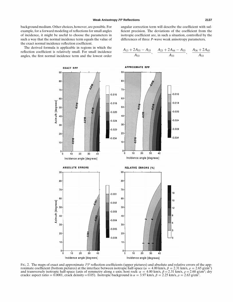
The values of the velocities and the density of the back-ground isotropic medium were determined by averaging [seeequations (32) and (33)]. For specific values, see the figure cap-tions. The results are displayed in the form of four plots shownin Figures 2–4. In all the plots, the horizontal axis correspondsto the angle of incidence θP, measured in degrees. The verticalaxis corresponds to the azimuth φ, also in degrees. As men-tioned above, the angles of incidence are considered only inthe limited interval (0◦, 42◦). Azimuth φ= 0◦ corresponds tothe profile along the axis of symmetry; azimuth φ= 90◦ corre-sponds to the profile in the plane perpendicular to the axis of

FIG. 1. Vertical sections of the P-wave phase velocity surfacescontaining the axes of symmetry for two dry crack models [withcrack density e= 0.05 (C) and e= 0.1 (D)].

symmetry, i.e., in the isotropy plane. The upper plots show ex-act and approximate RPP reflection coefficients; the lower plotsshow absolute and relative errors of the approximate formula.

From Figure 1, we can see that anisotropy in model A/C isnot too strong (about 12%). The contrast of velocities acrossthe reflector is always <10%, so we can expect a good per-formance of the approximate formula for this model. This isconfirmed by Figure 2. The relative error of the approximatelydetermined coefficient is always <3% for angles of incidence<20◦. For larger azimuths, this accuracy is guaranteed even forthe broader range of angles of incidence.

In model A/D (see Figure 3) the velocity contrast is slightlyhigher than in model A/C, but it never exceeds 12%. Aniso-tropy of the reflecting half-space is, however, much strongerthan in model A/C: it reaches nearly 20%. The relative errorsof the approximately determined coefficient are slightly higher;still, its fit with the exact coefficient is very good.

Figure 4 shows results for model B/D. In addition to stronganisotropy (nearly 20% as in Figure 3), we also deal with strongvelocity contrast (nearly 25%). Because the contrast is positive,a critical angle exists in this case. For the azimuth of 90◦, i.e., inthe plane of isotropy, the critical angle is about 50◦. For otherazimuths it will be slightly higher. This means the approximateformula for the reflection coefficient can be used only for angles<50◦. We can see in Figure 4 that the coefficients practicallydo not vary with azimuth for angles of incidence<25◦ becauseof the dominant role of the isotropic contrast for these angles.For angles of incidence>25◦, effects of anisotropy become ob-servable. In this region greater deviations of the approximatecoefficients from the exact ones can be observed. The devia-tions are larger for greater azimuths. This is because criticalangles for larger azimuths (close to the isotropy plane) appearfor lower values of the angles of incidence. The approximateformula works best for azimuths around 30◦. For lower az-imuths, it yields larger values than exact; for greater azimuths,it yields smaller values.

DISCUSSION AND CONCLUSIONS

A formula for PP reflection coefficient for weak contrastinterfaces separating two arbitrary weakly anisotropic mediawas derived. It was shown that the PP reflection coefficientdepends, among other things, on differences of 8 of the 14weak anisotropy parameters characterizing the phase veloc-ity and polarization vector of a P-wave in a weakly anisotropicmedium (see Psencık and Gajewski, 1998). In addition to theseparameters, the formula also depends on contrasts of param-eters characterizing vertical propagation of S-waves. The re-flection coefficient does not depend at all on the contrasts ofelastic parameters A14, A15, A24, A25, A34, A35, A46, and A56 ortheir combinations. Thus, these parameters can never be re-covered from the study of a PP reflection coefficient. Sincethe dependence of the reflection coefficient on the differencesof weak anisotropy parameters across an interface is linear, itoffers automatically an easy way to construct sensitivity oper-ators to determine these parameters in AVO (or AVA) studiesfrom the measured reflection coefficients.

The derived formulas do not depend only on differencesof elastic parameters across an interface but also depend onthe choice of the background medium. For this article, tradi-tional averaging was used to determine the parameters of the


background medium. Other choices, however, are possible. Forexample, for a forward modeling of reflections for small anglesof incidence, it might be useful to choose the parameters insuch a way that the normal incidence term equals the value ofthe exact normal incidence reflection coefficient.

The derived formula is applicable in regions in which thereflection coefficient is relatively small. For small incidenceangles, the first normal incidence term and the lowest order

FIG. 2. The maps of exact and approximate PP reflection coefficients (upper pictures) and absolute and relative errors of the app-roximate coefficient (bottom pictures) at the interface between isotropic half-space (α = 4.00 km/s, β = 2.31 km/s, ρ = 2.65 g/cm3)and transversely isotropic half-space (axis of symmetry along x-axis; host rock: α = 4.00 km/s, β = 2.31 km/s, ρ= 2.60 g/cm3; drycracks: aspect ratio = 0.0001, crack density= 0.05). Isotropic background is α = 3.97 km/s, β = 2.25 km/s, ρ = 2.63 g/cm3.

angular correction term will describe the coefficient with suf-ficient precision. The deviations of the coefficient from theisotropic coefficient are, in such a situation, controlled by thedifferences of three P-wave weak anisotropy parameters,

A13 + 2A55 − A33

A33,

A23 + 2A44 − A33

A33,

A36 + 2A45

A33


and two additional parameters,

A44 − A55

A33,

A45

A33.

Comparison with formulas for the P-wave phase velocityand polarization (see Psencık and Gajewski, 1998) show thatsmall-angle P-wave reflections are affected by the same weakanisotropy parameters. A similar conclusion holds for larger

FIG. 3. The same as in Figure 2, with isotropic half-space (α = 4.00 km/s, β = 2.31 km/s, ρ = 2.65 g/cm3) and transversely isotropichalf-space (axis of symmetry along x-axis; host rock: α= 4.00 km/s, β = 2.31 km/s, ρ = 2.60 g/cm3; dry cracks: aspect ratio= 0.0001,crack density= 0.1). Isotropic background is α= 3.95 km/s, β = 2.19 km/s, ρ= 2.63 g/cm3.

angles, for which the higher order angular correction term mustalso be considered.

We tested the accuracy of the derived formula on mod-els containing an interface separating an isotropic half-space,in which the incident wave propagates, from the transverselyisotropic half-space with the horizontal axis of symmetry. Wecalculated the reflection coefficient for all azimuths and a widerange of angles of incidence and compared the results withexactly calculated coefficients. Even if the velocity contrast


between the two half-spaces was rather strong (nearly 25%)and anisotropy of the reflecting half-space was also ratherstrong (nearly 20%), the approximate formula yielded verygood results.

To keep the paper reasonably short, we presented only theformula for the PP reflection coefficient. Derivation of theformula for the PP transmission coefficient is straightforwardfrom the presented equations (Psencık and Vavrycuk, 1998).

FIG. 4. The same as Figure 2, with isotropic half-space (α = 3.00 km/s, β = 1.73 km/s, ρ = 2.20 g/cm3) and transversely isotropichalf-space (axis of symmetry along x-axis; host rock: α = 4.00 km/s, β = 2.31 km/s, ρ = 2.60 g/cm3; dry cracks: aspect ratio= 0.0001,crack density = 0.1). Isotropic background is α = 3.45 km/s, β = 1.90 km/s, ρ = 2.40 g/cm3.

Derivation of R/T coefficients for converted waves is morecomplicated because of the appearance of angles 8 and 9

specifying the polarization vectors of S-waves in backgroundisotropic medium.

ACKNOWLEDGMENTS

The authors are grateful to V. Cerveny, L. Klimes, M.Slawinski, and an anonymous reviewer for their stimulating


reviews. This work was supported by the Grant Agency ofthe Czech Republic, grant no. 205/96/0968, and by the con-sortium project, Seismic Waves in Complex 3-D Structures(SW3D).”

REFERENCES

Aki, K., and Richards, P. G., 1980, Quantitative seismology: W.H.Freeman & Co.

Backus, G. E., 1965, Possible forms of seismic anisotropy of the upper-most mantle under oceans: J. Geophys. Res., 70, 3429–3439.

Banik, N. C., 1987, An effective parameter in transversely isotropicmedia: Geophysics, 52, 1654–1664.

Cerveny, V., 1982, Direct and inverse kinematic problems for inhomo-geneous anisotropic media—Linearization approach: Contr. Geo-phys. Inst. Slov. Acad. Sci., 13, 127–133.

Daley, P. F., and Hron, F., 1977, Reflection and transmission coeffi-cients for transversely isotropic media: Bull. Seismol. Soc. Am., 67,661–675.

Gajewski, D., and Psencık, I., 1987, Computation of high-frequencyseismic wavefields in 3-D laterally inhomogeneous anisotropic me-dia: Geophys. J. R. Astr. Soc., 91, 383–411.

Haugen, G. U., and Ursin, B., 1996, AVO-A analysis of vertically frac-tured reservoir underlaying shale: Presented at the 66th Ann. Inter-nat. Mtg., Soc. Expl. Geophys., Expanded Abstracts, 1826–1829.

Hearn, A. C., 1991, Reduce 3.4. User’s manual: Rand Corp.,Hudson, J. A., 1981, Wave speeds and attenuation of elastic waves

in material containing cracks: Geophys. J. R. Astr. Soc., 64,133–150.

Jech, J., and Psencık, I., 1989, First-order perturbation method foranisotropic media: Geophys. J. Internat., 99, 369–376.

Keith, C. M., and Crampin, S., 1977, Seismic body waves in anisotropicmedia: Reflection and refraction at a plane interface: Geophys. J.Roy. Astr. Soc. 49, 181–208.

Psencık, I., and Gajewski, D., 1998, Polarization, phase velocity andNMO velocity of qP waves in arbitrary weakly anisotropic media:Geophysics, 63, 1754–1766.

Psencık, I., and Vavrycuk, V., 1998, Weak contrast PP wave displace-ment R/T coefficients in weakly anisotropic elastic media: Pageoph,151, 699–718.

Rueger, A., 1996, Analytic description of reflection coefficients inanisotropic media: 58th Ann. Mtg., Eur. Assn. Geoscientists andEngineers, Extended Abstracts, 1, P026.

——— 1997, P-wave reflection coefficients for transversely isotropicmodels with vertical and horizontal axis of symmetry: Geophysics,62, 713–722.

Thomsen, L., 1986, Weak elastic anisotropy: Geophysics, 51, 1954–1966.

——— 1993, Weak anisotropic reflections, in Castagna, J. P., andBackus, M. M., Eds., Offset-dependent reflectivity—Theory andpractice of AVO analysis: Soc. Expl. Geophys., 103–111.

Tsvankin, I., 1996, P-wave signatures and parameterization of trans-versely isotropic media: An overview: Geophysics, 61, 467–483.

Ursin, B., and Haugen, G. V., 1996, Weak-contrast approximation ofthe elastic scattering matrix in anisotropic media: Pageoph, 148, 685–714.

Zillmer, M., Gajewski, D., and Kashtan, B. M., 1997, Reflection co-efficients for weak anisotropic media: Geophys. J. Internat., 129,389–398.

——— 1998, Anisotropic reflection coefficients for a weak-contrast in-terface: Geophys. J. Internat., 132, 159–166.

APPENDIX

SLOWNESS AND POLARIZATION VECTORS OF INCIDENT AND UNCONVERTEDTRANSMITTED P-WAVES IN WEAKLY ANISOTROPIC MEDIA

The slowness vector p(0)i of the incident P-wave propagat-

ing in a weakly anisotropic medium whose direction coincideswith the direction of the slowness vector p0(0)

i in the backgroundmedium can be written as

p(0)i = p0(0)

i + δp(0)i = p0(0)

i

(1− α−1δc(0)). (A-1)

Here δc(0) denotes a deviation of the phase velocity of theincident wave from the phase velocity in the backgroundmedium. The deviations δc(0) and similarly δc(6) for the trans-mitted P-wave, which will be needed later, are given by thewell-known formula (Backus, 1965; Cerveny, 1982; Jech andPsencık, 1989),

δc(0) = 12αδa

(1)i jkl p0(0)

i g0(0)j g0(0)

k p0(0)l ,

(A-2)

δc(6) = 12αδa

(2)i jkl p0(0)

i g0(0)j g0(0)

k p0(0)l .

For the determination of the slowness vector p(6)i of the trans-

mitted P-wave, we use equation (4). The tangential projectionbi of the slowness vector into the interface6 can be determinedfrom equations (5) and (A-1) as

bi = b0i + δbi

= [p0(0)i − (p0(0)

k νk)νi]− α−1δc(0)[p0(0)

i − (p0(0)k νk

)νi].

(A-3)

The projection ξ (6) of the slowness vector into the normal νi tothe interface 6 can be determined from the eikonal equation,

a(2)i jkl p(6)

i p(6)l g(6)

j g(6)k = 1, (A-4)

which simply follows from the Christoffel equation (7). In aweakly anisotropic medium, equation (A-4) can be expandedas

a0i jkl p0(0)

i p0(0)l g0(0)

j g0(0)k + δa(2)

i jkl p0(0)i p0(0)

l g0(0)j g0(0)

k

+ 2a0i jkl δbi p0(0)

l g0(0)j g0(0)

k + 2a0i jkl δξ

(6)νi p0(0)l g0(0)

j g0(0)k = 1.

(A-5)

Here δbi and δξ (6)νi are the deviations of the tangent and nor-mal components of the slowness vector of the transmitted wavein the weakly anisotropic medium from the same componentsin the background isotropic medium. The deviation δbi given inequation (A-3); δξ (6)νi can be determined from equa-tion (A-5). Using equations (13), (20), (21), (A-2) and (A-3) inequation (A-5), we get, after some manipulation,

δξ (6) = δc(0)[1− α2

(νk p0(0)

k

)2]− δc(6)

α3(νk p0(0)

k

) . (A-6)

Using equations (A-3) and (A-6), we can write the final formulafor the slowness vector of the transmitted wave in a weakly


anisotropic medium as

p(6)i = p0(0)

i + δp(6)i

= p0(0)i −

[α−1 p0(0)

i δc(0) +(δc(6) − δc(0)

)α3(νk p0(0)

k

) νi

]. (A-7)

The polarization vector of the incident or transmitted P-wave propagating in the weakly anisotropic medium can be de-termined from formulas presented by Jech and Psencık (1989).For a given slowness vector, the polarization vector of theP-wave is given as the sum of a unit vector in the directionof the slowness vector and a perturbation. We can write

g(0)i = g0(0)

i + δg(0)i , g(6)

i = g0(6)i + δg(6)

i , (A-8)

where g0(0)i is given in equation (21) and g0(6)

i can be ob-tained by normalization of the slowness vector p(6)

i given in

equation (A-7),

g0(6)i = αp0(0)

i + (δc(6) − δc(0))(p0(0)i − νi

α2(νk p0(0)

k

)).

(A-9)

The perturbations δg(N)i , N = 0, 6, in equation (A-8) are (Jech

and Psencık, 1989)

δg(0)m =

α

α2 − β2δa(1)

i jkl p0(0)i g0(0)

j g0(0)k

(δlm − g0(0)

l g0(0)m

),

(A-10)

δg(6)m =

α

α2 − β2δa(2)

i jkl p0(0)i g0(0)

j g0(0)k

(δlm − g0(0)

l g0(0)m

).

The determination of the amplitude-normalized tractions inweakly anisotropic media is straightforward. It can be ob-tained by inserting expressions (13), (A-1), (A-7), and (A-8)into equation (9).

pp-wave reflection coefficients in weakly anisotropic

Documents