arX

iv:1

808.

0766

6v3

[he

p-ph

] 8

Jan

202

0

The Tsallis Entropy and the BKT–like Phase Transition in the Impact Parameter

Space for pp and pp Collisions

S. D. Campos,∗ V. A. Okorokov,† and C. V. Moraes∗∗Departamento de Física, Química e Matemática,

Universidade Federal de São Carlos, 18052-780, Sorocaba, SP, Brazil and†National Research Nuclear University MEPhI (Moscow EngineeringPhysics Institute), Kashirskoe highway 31, 115409 Moscow, Russia

(Dated: January 9, 2020)

In this paper, one uses the Tsallis entropy in the impact parameter space to study pp and pp

inelastic overlap function and the energy density filling up mechanism responsible by the so-calledblack disk limit as the energy increases. The Tsallis entropy is non-additive and non-extensiveand these features are of fundamental importance since the internal constituents of pp and pp arestrongly correlated and also the existence of the multifractal character of the total cross-section. Theentropy approach presented here takes into account a phase transition occurring inside the hadronsas the energy increases. This phase transition in the impact parameter space is quite similar to theBerezinskii–Kosterlitz–Thouless phase transition, possessing also a topological feature due to themultifractal dimension of the total cross-sections in pp and pp scattering.

PACS numbers: 13.85.Dz;13.85.Lg

I. INTRODUCTION

The transition point separating two different states of matter is known as a phase transition and is observed when aphysical system suddenly changes its macroscopic behavior due to a smooth variation of the order parameter passingthrough its critical value. In the classical point of view, the temperature is usually the driving parameter of suchtransitions and determines exactly the phase transition by heat transfer. Both the superfluid helium and the Ginzburg–Landau superconducting model are very well-known examples where phase transitions are thermal-dependent in theclassical sense. In the quantum world at zero temperature, the tuning parameter is chosen depending on the experiment(for instance, the magnetic field, chemical potential or electric field), and in these systems, the phase transition isknown as the quantum phase transition [1].

In a modern view, phase transitions (classical or quantum) are classified as first-order or second-order. The first-order phase transition is determined by the discontinuity at first derivative of a relevant thermodynamic potentialand, as consequence, such phase transition can also be called as discontinuous one, from the point of view of thebehavior for the first derivative of the thermodynamic potential. The second-order phase transition is continuousat the first derivative and divergent at higher order derivatives, and such phase transition can also be called ascontinuous one. Despite the significant progress in the study of critical phenomena there some disagreements withregard to terminology. For instance, the classification of phase transitions as first-order or continuous is justified in [2].However, such classification seems self-contradictory because uses different categories, namely, "order" and the feature(continuity/discontinuity) in the behavior of the first derivative of a relevant thermodynamic potential. Therefore thewell-known classification as first- /second-order [3] is used for phase transitions in this paper. In any classification,the so-called critical point separates the system ordering from a symmetric state to a broken-symmetry state.

The Berezinskii–Kosterlitz–Thouless (BKT) phase transition [4, 5], whose main goal is the study of correlationsbetween pairs of topological defects (vortex-antivortex), is an example from a geometrical point of view. In condensedmatter physics, the study of such transition is a tool to understand how collective coherent phenomena (a topologicaldefect) can emerge from certain structures and how it can be connected to another one in a different space. If theinteraction between topological defects depends on the logarithm of the spatial separation, then the BKT phasetransition takes place being used to explain the phenomenon. As will show later, the model proposed here presents aBKT-like phase transition.

As well-known, phase transitions are closely connected to the entropy of a system and to the Helmholtz free energy,which is nothing more than the useful work that can be extracted from a closed thermodynamic system at a constant

∗Electronic address: sergiodc@ufscar.br†Electronic address: VAOkorokov@mephi.ru; Okorokov@bnl.gov

2

temperature. In general, one applies the Boltzmann entropy (extensive) to this kind of systems. However, a non-extensive form of entropy based on the q-Gaussian was proposed and successfully used to calculate and explain somephysical properties in several systems, in particular, those with fractal properties. This is the so-called Tsallis entropy(TE) [6]. Notice that in the last decades, various approaches have been used to calculate the entropy of systems,presenting interesting properties. The Shannon entropy [7], the Rényi entropy [8], and the von Neumann entropy[9] are examples of such calculation approaches, each one applied to a specific physical problem. However, all theseformulations can be reduced to the TE [10].

Entropy is one of the most important physical quantities in thermodynamics and cannot be put aside in any reliablemodel, even when its results are disconcerting in the classical world [11]. Moreover, entropy cannot only be viewedas the disorder of a given system. Since the fundamental work of Shannon [7], the entropy have been also relatedto the amount of information we can attain from the system. It should be stressed that the applicability of suchquantity as "entropy" for the study of an interaction process between atomic nuclei and particles requires a detailedand rigorous justification. Here one can note the following with regard of two main problems: (i) a finite number ofparticles in the system under consideration and (ii) the time T invariance in the quantum field theory (QFT). Firstof all, the usual way to use entropy is by assuming some large statistical ensemble (canonical, for instance). In theclassical view, the number of elements in such an ensemble is at least of the order of the Avogadro number. However,there are filtering methods used in information theory to reduce the number of bits, allowing at least an estimationto the entropy. Then, the size of the ensemble is not a problem, at first glance. Of course, if the size of the ensemblegrows, then the estimation may also tend to a "better" value [12]. Second, indeed, the entropy almost always grows.Nevertheless, there are some systems where the entropy achieves negative values. The concept of negative absolutetemperature can be applied in such systems [11]. In these systems, the arrow of time is the same, but a non-trivialinterpretation must be used to explain the result. So, the T invariance of the QFT is preserved and, in particular,the strong interactions are in a safe place.

The calculation of the entropy is a complicated task but can provide remarkable results as the proton and electronradii in the nucleus [13]. The z-scaling also can be used to furnish the entropy in a system with particle production [14]and further be calculated in D-branes [15]. All these approaches used to evaluate the entropy reveal some particularthermodynamics aspect of the system under study.

Recently, the concept of fractal dimensions was introduced in the study of pp and pp total cross sections [16, 17].These fractal dimensions were used to explain the transition from a decreasing total cross section for an increasing oneas the energy tends to infinity. The fractal dimensions emerging in these pictures are energy-dependent in the sensethat for the decreasing total cross section as the energy grows up to a critical value one obtains a negative fractaldimension, and for the increasing total cross section, one has a positive fractal dimension. On the other hand, in termsof momentum space (or in configuration space), an attempt to connect the intermittency pattern [18–22] in hadroniccollisions to fractal dimensions uses a second-order phase transition [23–26]. The approach presented in [27] showsthis possibility through the use of thermofractals. It should be stressed, however, that in the energy-momentum spacea system with a particular fractal structure can also be described by the Tsallis statistics. In particular, this system isscale-free and can be used to study the similarities between the nonextensitiy in hadron systems and the Hagedorn’sfireballs, for instance. The intermittency effects can be used to study fractal-like properties of several systems as, forinstance, the multiparticle production [28, 29], and the gluon emission resulting from the QCD evolution equation[30]. The fractal structure in the energy-momentum space can also be used to study scaling properties through theCallan-Symanzik renormalization group equation [31, 32].

In the present paper, is proposed a naive model to evaluate the entropy of pp and pp elastic scattering adoptingsubtleties assumptions. These assertions allow the connection of the TE and the inelastic overlap function in theimpact parameter space, providing a novel interpretation of the energy density filling up mechanism of the hadron asthe collision energy increases. This process can enhance the understanding of how the black disk limit is achieved (ornot).

The paper is organized as follows. In section II the impact parameter space basic formalism is presented. Insection III only the essential of the TE is presented as well as our model. Section IV present a basic example ofan application using the most general experimental results and phenomenological approaches to the inelastic overlapfunction. Section V presents critical remarks about the results.

II. IMPACT PARAMETER POINT OF VIEW

The impact parameter space is the right place to study the fractal behavior of pp and pp since it allows a generalview of the elastic and inelastic scattering channels. In this way, using the impact parameter formalism, the fractaldimensions obtained in [16, 21–26] may be viewed as a consequence of a phase transition in pp and pp elastic scatteringindicating a geometric phase transition. This topological phase transition taking place inside the hadron may be

3

responsible be a change in the energy density filling up mechanism, allowing the emergence of fractal structures inthe total cross section.

The impact parameter is very useful as a geometrical viewpoint of the scattering process. The squared momentumtransfer −t = |t| is replaced by its conjugate variable b, the transverse distance between the colliding particles inimpact parameter space. In this space, the analytic function F (s, t) = ReF (s, t) + iImF (s, t) representing the elasticscattering is written at a fixed s as

F (s, t) = i4πs

∫ ∞

0

db bJ0(b√

|t|)Γ(s, b) = i4πs

∫

0

∞

db bJ0(b√

|t|)

1− exp[iχ(s, b)]

, (1)

where J0(x) is a zeroth order Bessel function, Γ(s, b) = ReΓ(s, b)+ iImΓ(s, b) = 1− exp[iχ(s, b)] is the profile functionand χ(s, b) is the eikonal written as χ(s, b) = Reχ(s, b)+ iImχ(s, b). The unitarity condition connects the total (σtot),elastic (σel) and inelastic (σin) cross sections new the profile function and can be written in b-representation as

2ReΓ(s, b) =∣

∣Γ(s, b)∣

∣

2+Ginel(s, b), (2)

where Ginel(s, b) is the inelastic overlap function [33] and∣

∣Γ(s, b)∣

∣

2represents the shadow contribution of the elastic

channel

σtot(s) = 2

∫

d2bReΓ(s, b), σel(s) =

∫

d2b∣

∣Γ(s, b)∣

∣

2, σin(s) =

∫

d2bGinel(s, b). (3)

Here it is used the optical theorem s−1ImF (s, 0) = σtot(s) [34, 35]. Also the unitarity condition demands Imχ(s, b) ≥ 0,implying that Ginel(s, b) represents the probability of an elastic scattering in the 2D kinematic space (s, b) and thisquantity is given by [36]

Ginel(s, b) = 1− exp[

−2Imχ(s, b)]

≤ 1. (4)

As usual, one can introduce the opacity Ω(s, b) defined as Ω(s, b) = 2Imχ(s, b). It is well-known that the opacitymeasures the matter density distribution inside the incident particles. At lower energies [37], the opacity presentsa Gaussian shape not observed in LHC data, whose indication is the growth of opacity at small b as presented inTOTEM data [38]. The inelastic profile function, on the other hand, determines how absorptive is the interactionregion (inelastic) depending on b. When Ginel(s, b) = 0 the object is called transparent and to Ginel(s, b) = 1, theabsorption is maximal. Theoretically the latter result, in general, occurs at b = 0 fm in the asymptotic conditions → ∞. Notwithstanding, in [39, 40] there is an approach indicating that at b = 0 fm, the black disk limit is notachieved. Indeed, the black disk picture seems to be achieved at some critical bc, near forward direction, indicatingthe arising of a gray area [39, 40]. This model was further analyzed in [41–48] resulting in the so-called hollownesseffect near the forward direction.

Using the Fourier–Bessel transform of the amplitude (1) one can write the dimensionless profile function as

Γ(s, b) =−i

8π

∫ ∞

0

d|t|J0(b√

|t|)F (s, t)

s≡ −i

8πF (s, b). (5)

Neglecting derivative dispersion contributions, one can suggest that the t-dependence is taken into account by only onereal function f(s, t), which is common for both real and imaginary part of F (s, t). Thus, ReF (s, t) = ReF (s, 0)f(s, t)and ImF (s, t) = ImF (s, 0)f(s, t). Also the last relations imply f(s, 0) = 1. Note that for small |t| (large b) inside theLehmann–Martin ellipse, f(s, t) can be taken in a first approximation as the same function for the real and imaginarypart of the elastic scattering amplitude, as can be viewed in [49]. For large |t| (small b), f(s, t) is also approximatelythe same for ReF (s, t) and ImF (s, t). Moreover, it should be stressed that we are mostly interested here in the large|t| region (small b). Then

ReΓ(s, b) =1

8π

ImF (s, 0)

s

∫ ∞

0

d|t|J0(b√

|t|)f(s, t) = σtot

8πf(s, b), (6a)

ImΓ(s, b) = − 1

8π

ReF (s, 0)

s

∫ ∞

0

d|t|J0(b√

|t|)f(s, t) = −ρσtot

8πf(s, b) ≡ −ρReΓ(s, b), (6b)

where ρ(s) ≡ ReF (s, 0)/ImF (s, 0) is the ratio of the real to imaginary part of the amplitude in the forward direction.It should be noted that experimental data show |ρ(s)| . 0.3 (0.2) at

√s & 5 (3) GeV for pp (pp) collisions. Therefore

4

one can neglect the ReF (s, t) with respect of the ImF (s, t) and, as consequence, the ImΓ(s, b) with respect to ReΓ(s, b)at accuracy level not worse than 0.3 (0.2) in the energy domains indicated above for pp and pp collisions [17]. Basedon the equations (6a) and (6b) one can derive for the inelastic overlap function

Ginel(s, b) = ReΓ(s, b)

2− ReΓ(s, b)[1 + ρ2(s)]

≈ ReΓ(s, b)

2− ReΓ(s, b)

, (7)

where the approximate relation is valid at accuracy level not worse than 0.09 (0.04) in wide energy domain√s & 5 (3)

GeV for pp (pp) collisions.It should be noted that the results obtained above are derived with the help of the most general property of quantum

field theory, namely, unitarity condition and, consequently, they are model independent.

III. THE TSALLIS ENTROPY

Although entropy is a well-defined quantity in physics its calculation depends on the presence or not of correlationsamong the components of the lattice, for instance. The internal structure of the hadron grows in complexity as theenergy increases, possibly showing a black disk picture as s → ∞, where s is the squared-energy in the center-of-masssystem. This result prevents the use of the Boltzmann entropy since the correlation between the constituents of thehadron grows as s increases due to the confinement potential. Accordingly, the use of the TE may furnish a betterunderstanding of the internal structure of the hadron than the Boltzmann one.

Note that the Boltzmann entropy (SB) assumes each part of the lattice as an independent system with a definedentropy, and the sum of all cells results in the total entropy of the system. Then, this entropy is additive, i.e., for asystem composed of a countable number of subsystems i = 1, 2, ...,W each one with entropy Si the total entropy isgiven by

SB =

W∑

i=1

Si. (8)

Indeed, if the subsystems have no correlations at all or only local correlations, then SB is also extensive [6]. However,if there are correlations between the cells the Boltzmann entropy is no longer valid and the entropy of each cell cannotbe computed separately and consequently, the total entropy is not the sum of each cell of the lattice. Of course, ifthe correlations are weak, then the Boltzmann entropy can be used as a first approximation to solve the problem. Analternative approach, however, which takes into account the correlations is provided by the TE (ST ) [6]. In a singlesystem composed of two subsystems a and b it is written as

ST = Sa + Sb + (1− w)SaSb, (9)

where w is the entropic index. If w 6= 1, then ST is non-additive as well as non-extensive. On the other hand, ifw = 1, the TE is reduced to the Boltzmann entropy one. Thus, w characterizes the degree of non-extensivity ofthe system. It is important to stress this kind of entropy calculation is applicable when the system exhibits somelong-range correlations, intrinsic fluctuations or fractal structure in phase space [50]. Thus one notes, in the fieldof high energy physics the non-extensivity of the system of secondary particles can be provided by event-by-eventfluctuations of some parameter that can be associated with the temperature of part of the system acting as a heatbath [51]. Such fluctuations can lead to the violation of the strong system independence (SSI) and, consequently, tothe appearance of non-extensive entropy classes, in particular, of ST . Therefore, in general, the ST can be emergedin high-energy collisions due to either physical or statistical (a relatively small number of elements in the subsystem– heat bath) reasons. An additional study and justification may be required for a conclusion about the reason for ST

appearance in some interaction cases between particles and nuclei. The continuous form of the TE is given by [52]

ST (p, w) =1

w − 1

(

1−∫ ∞

−∞

[

p (x)]w

dx

)

, (10)

where p (x) is the probability density function. The existence of fractal structures in the momentum and in the energyspace for both pp and pp collisions may allow the use of the TE to study how these fractal dimensions can contributeto the understanding of the collision process. Additionally, if one looks to the entropy as the information that maybe gained observing a physical quantity depending on (s, b) in the impact parameter space, then b may be used as ameasure of this information and how it acts on the black disk picture.

5

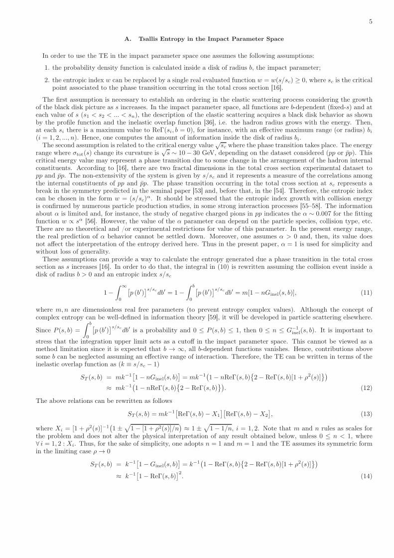
A. Tsallis Entropy in the Impact Parameter Space

In order to use the TE in the impact parameter space one assumes the following assumptions:

1. the probability density function is calculated inside a disk of radius b, the impact parameter;

2. the entropic index w can be replaced by a single real evaluated function w = w(s/sc) ≥ 0, where sc is the criticalpoint associated to the phase transition occurring in the total cross section [16].

The first assumption is necessary to establish an ordering in the elastic scattering process considering the growthof the black disk picture as s increases. In the impact parameter space, all functions are b-dependent (fixed-s) and ateach value of s (s1 < s2 < ... < sn), the description of the elastic scattering acquires a black disk behavior as shownby the profile function and the inelastic overlap function [36], i.e. the hadron radius grows with the energy. Then,at each si there is a maximum value to ReΓ(si, b = 0), for instance, with an effective maximum range (or radius) bi(i = 1, 2, ..., n). Hence, one computes the amount of information inside the disk of radius bi.

The second assumption is related to the critical energy value√sc where the phase transition takes place. The energy

range where σtot(s) change its curvature is√s ∼ 10− 30 GeV, depending on the dataset considered (pp or pp). This

critical energy value may represent a phase transition due to some change in the arrangement of the hadron internalconstituents. According to [16], there are two fractal dimensions in the total cross section experimental dataset topp and pp. The non-extensivity of the system is given by s/sc and it represents a measure of the correlations amongthe internal constituents of pp and pp. The phase transition occurring in the total cross section at sc represents abreak in the symmetry predicted in the seminal paper [53] and, before that, in the [54]. Therefore, the entropic indexcan be chosen in the form w = (s/sc)

α. It should be stressed that the entropic index growth with collision energyis confirmed by numerous particle production studies, in some strong interaction processes [55–58]. The informationabout α is limited and, for instance, the study of negative charged pions in pp indicates the α ∼ 0.007 for the fittingfunction w ∝ sα [56]. However, the value of the α parameter can depend on the particle species, collision type, etc.There are no theoretical and /or experimental restrictions for value of this parameter. In the present energy range,the real prediction of α behavior cannot be settled down. Moreover, one assumes α > 0 and, then, its value doesnot affect the interpretation of the entropy derived here. Thus in the present paper, α = 1 is used for simplicity andwithout loss of generality.

These assumptions can provide a way to calculate the entropy generated due a phase transition in the total crosssection as s increases [16]. In order to do that, the integral in (10) is rewritten assuming the collision event inside adisk of radius b > 0 and an entropic index s/sc

1−∫ ∞

0

[

p (b′)]s/sc

db′ = 1−∫ b

0

[

p (b′)]s/sc

db′ = m[1− nGinel(s, b)], (11)

where m,n are dimensionless real free parameters (to prevent entropy complex values). Although the concept ofcomplex entropy can be well-defined in information theory [59], it will be developed in particle scattering elsewhere.

Since P (s, b) =

∫ b

0

[

p (b′)]s/sc

db′ is a probability and 0 ≤ P (s, b) ≤ 1, then 0 ≤ n ≤ G−1

inel(s, b). It is important to

stress that the integration upper limit acts as a cutoff in the impact parameter space. This cannot be viewed as amethod limitation since it is expected that b → ∞, all b-dependent functions vanishes. Hence, contributions abovesome b can be neglected assuming an effective range of interaction. Therefore, the TE can be written in terms of theinelastic overlap function as (k ≡ s/sc − 1)

ST (s, b) = mk−1[

1− nGinel(s, b)]

= mk−1(

1− nReΓ(s, b)

2− ReΓ(s, b)[1 + ρ2(s)])

≈ mk−1(

1− nReΓ(s, b)

2− ReΓ(s, b))

. (12)

The above relations can be rewritten as follows

ST (s, b) = mk−1[

ReΓ(s, b)−X1

][

ReΓ(s, b)−X2

]

, (13)

where Xi = [1 + ρ2(s)]−1(

1 ±√

1− [1 + ρ2(s)]/n)

≈ 1 ±√

1− 1/n, i = 1, 2. Note that m and n rules as scales forthe problem and does not alter the physical interpretation of any result obtained below, unless 0 ≤ n < 1, where∀ i = 1, 2 : Xi. Thus, for the sake of simplicity, one adopts n = 1 and m = 1 and the TE assumes its symmetric formin the limiting case ρ → 0

ST (s, b) = k−1[

1−Ginel(s, b)]

= k−1(

1− ReΓ(s, b)

2− ReΓ(s, b)[1 + ρ2(s)])

≈ k−1[

1− ReΓ(s, b)]2. (14)

6

The above result furnishes a measure of the entropy in the impact parameter space through the use of the inelasticoverlap function. It is known that Ginel(s, b) can be evaluated with the help of some model–dependent technique.Therefore the ST (s, b) defined by the relations (12) – (14) is model–dependent in general. The signature (positive ornegative) of the TE reveals an s-dependence analyzed as follows. Considering s < sc, the signature of ST is negativeand it can be interpreted as the system using the energy of the beam to self-organize or maintain its internal structure(quarks and gluons). Then, as s increases the entropy tends to a maximum by negative values, i.e. the system tendsto achieve the maximum of its self-organization as well. Moreover, using a simple fitting model written as

σtot(s) = γ1 ln(s/sc)γ2 (15)

where γ1 and γ2 are free fit parameters, being γ2 the Hausdorff–Besicovitch fractal dimension, a novel interpretationfor the total cross section was proposed in [16] where the fractal dimension in this energy range is negative anddifferent to pp and pp, producing distinct patterns to Ginel(s, b). Hence, the measure of the emptiness of pp and pptotal cross section results in different values to ST .

The negative entropy and the negative fractal dimensions imply the constituents, the internal arrangement to pp andpp are unlike, i.e. the quark-quark and quark-gluon arrangement of the proton are different of the antiquark-antiquarkand antiquark-gluon arrangement of the antiproton. In the popular picture, one says that the odderon distinguishesparticle from antiparticle.

When the energy s grows and go through the transition point sc, the TE turns positive and stands for the systemgrowing disorder. As obtained in [16], the total cross section to pp and pp possesses positive fractal dimensions tos > sc and both tends to the same value as s → ∞. Both results have shown that at high energies the arrangement ofthe internal constituents to pp and pp tends to the same behavior. Then, the pomeron does not distinguish particlefrom antiparticle.

The different internal arrangement of proton and antiproton may absorb the incoming energy by distinct mecha-nisms. As pointed out [16], the negative fractal dimension represents the emptiness of the hadron internal arrangementand the total cross section is a measure of that. The internal arrangement of quarks and gluons at lower energies inthe proton picture is less empty than the arrangement of the antiquarks and gluons inside the antiproton, as can beviewed in the total cross section experimental dataset for s < sc.

At the transition point, (s = sc) the fractal dimension to pp and pp total cross section is null and the systemachieves its maximum capability to convert the absorbed energy in order. This point may indicate the first saturationpoint in pp and pp total cross section dataset. It is interesting to note that pp and pp total cross section tends to thesame saturation point sc, possibly indicating this value as a universal character of total cross sections.

Above the critical point, (s > sc), the internal constituents of pp and pp achieve degrees of freedom previouslyblocked by using the energy coming from the beam converted in thermal agitation resulting in the rise of the totalcross-section as s increases.

The above scenarios introduced by the TE and by the fractal dimension concept result in the question of howoccurs the filling up mechanism responsible by the black disk behavior of pp and pp as s → ∞. A possible answeris given as follows. As well-known, in QCD the confinement of quarks and gluons prevent its freedom below theHagedorn temperature [60], where the hadrons are no longer stable. However, the increasing energy of the scatteringimply in the enhanced of the thermal bath at each particle is subject. This energy is then transferred to the internalconstituents of the proton and antiproton by a heat transport mechanism.

The zero entropy state can be established when at nGinel(s, b) = 1 for some particular (s, b). As well-known, zeroentropy occurs when a system achieves its ground-state (or its maximum self-organization state). Thus, at this point,the physical state of the system is completely known (the ways one can arrange its internal configuration is exactlyone). The general belief is that nGinel(s, b) = 1 is achieved in the asymptotic limit s → ∞ and at b = 0. Then, fromsome s sufficiently high the energy of both pp and pp possess the same behavior at b = 0. However, there exist somemodels indicating this result may be achieved at some b 6= 0 [41, 61]. The implication of that is the appearance of agray area in the inelastic overlap function near b = 0.

It is interesting to note that the first equation in the chain (12) can also be written assuming only as the first orderof the logarithm expansion below

ST (s, b) = −mk−1 ln[

nGinel(s, b)]

, (16)

implying higher orders are corrections for equation (12). In addition, if the logarithm of the inelastic overlap functionis connected to the pair spatial separation of the constituents of the hadron, then it can represent the interactionof topological defects [4, 5] inside the hadron. As well-known, in the BKT phase transition, the entropy dependson the logarithm of the spatial pair separation of vortices. On the other hand, it has been shown that the correctdescription of the inelastic overlap function needs at least two Gaussian [62]. If one associate each Gaussian to aparticular location inside the hadron, then the TE given by equation (16) may be interpreted as a BKT-like phase

7

transition occurring inside the hadron at s = sc, being sc the critical squared energy value where the total crosssection experimental dataset change its curvature.

IV. BASIC APPLICATION: GENERAL FORM FOR THE OVERLAP FUNCTION

In this section one focus on recent inelastic overlap function models comparing the results by using ST . Thesecomparisons may furnish a better understanding of how entropy is released in each model. There is a wide set ofmodels for nucleon-nucleon elastic scattering and, therefore, it seems reasonable to discuss only those based on themost general and basic statements of the Axiomatic Quantum Field Theory (AQFT). In the present paper, the (a)unitarity condition and (b) asymptotic theorems are the basic ground.

A. Non-central collisions (b 6= 0)

The most general and well-established experimental result for elastic scattering is the fast decreasing of the differ-ential cross section (dσ/dq2) with the increasing |t| ≃ q2 in the diffraction peak. As a first approximation, the dσ/dq2

shows an exponential growth with the slope B(s) at q2 under consideration. Thus, one writes for the t-dependentpart of scattering amplitude f(s, t) = exp[B(s)|t|/2] and

f(s, b) =

∫ ∞

0

d|t|J0(b√

|t|) exp[

B(s)|t|2

]

≈ 2

∫ ∞

0

dq qJ0(bq) exp

[

−B(s)q2

2

]

=2

B(s)exp

[

− b2

2B(s)

]

. (17)

Then

ReΓ(s, b) =[

σtot/4πB(s)]

exp[

−b2/2B(s)]

≡ ζ(s) exp[

−b2/2B(s)]

, (18a)

ImΓ(s, b) =[

−ρσtot/4πB(s)]

exp[

−b2/2B(s)]

≡ −ρ(s)ζ(s) exp[

−b2/2B(s)]

, (18b)

where ζ is the parameter defined as following

ζ(s) =σtot(s)

4πB(s)=

4σel(s)

[1 + ρ2(s)]σtot(s)≈ 4σel(s)

σtot(s). (19)

Note that at ζ = 1 the Ginel(s, b) represent a black disk and for ζ 6= 1 the inelastic overlap function diminishes.Moreover, the position of the maximum b2max = 2B ln ζ with the full absorption Ginel(s, bmax) = 1 depends on B(s)and ζ(s).

Taking into account (7) and (12) one can deduce the final expressions for both the inelastic overlap function andthe TE, respectively, within a general phenomenological way for the scattering amplitude

Ginel(s, b) = ζ(s) exp[

−b2/2B(s)]

2− ζ(s) exp[

−b2/2B(s)]

[1 + ρ2(s)]

≈ ζ(s) exp[

−b2/2B(s)]

2− ζ(s) exp[

−b2/2B(s)]

, (20)

ST (s, b) = mk−1(

1− nζ(s) exp[

−b2/2B(s)]

2− ζ(s) exp[

−b2/2B(s)]

[1 + ρ2(s)])

≈ mk−1(

1− nζ(s) exp[

−b2/2B(s)]

2− ζ(s) exp[

−b2/2B(s)]

). (21)

B. Central collisions (b = 0)

The general equations (20) and (21) are obtained assuming the most general phenomenological view for the dif-

ferential cross section dσ/dq2 =[

ImF (s, 0)/4√πs

]2exp

[

−B(s)q2/2]

. However, the concrete form for the energydependence of both the Ginel(s, b) and the ST (s, b) is driven by the corresponding dependence for scattering param-eters. The exact relations in (20), (21) are defined by energy dependencies for global scattering parameters σtot, ρand for the slope B, while the corresponding approximate relations depend on the ratio Re/t = σel/σtot and B. Theforward condition b = 0 allows the exclusion of the dependence on B(s). In this specific case, ReΓ(s, 0) = ζ(s) and

8

ImΓ(s, 0) = −ρ(s)ζ(s). Considering exactly central collision with b = 0 one obtains from the general relations (20),(21) the following results

Ginel(s, 0) = ζ(s)

2− ζ(s)[1 + ρ2(s)]

≈ ζ(s)

2− ζ(s)

, (22)

ST (s, 0) = mk−1

1− nζ(s)[

2− ζ(s)(1 + ρ2(s))]

≈ mk−1

1− nζ(s)[

2− ζ(s)]

. (23)

The symmetric form for the TE in central collisions

ST (s, 0) = k−1[

1− ζ(s)]2

(24)

derived from (23) can also be viewed as the first order approximation of the logarithm series ST (s, 0) = k−1 ln2 ζ.Thus, for exactly central pp and pp collisions, only energy dependence for Re/t remains, which varies in different

models. Detailed analysis of this dependence for pp and pp scattering as well as for joined sample for these collisions1

is made in [63] with the help of the fitting of experimental data by an empirically chosen function.In general, the asymptotic value ζ(s)|s→∞ varies from one approach to another due to model-dependent value

of Re/t for s → ∞. The result from [63], obtained with the help of asymptotic theorems and assumptions for theproperties of scattering amplitude for binary process 1 + 2 → 3 + 4 within AQFT, assumes that ζ(s)|s→∞ → 3.The approach of partonic disks [64] provides some faster growth of the ratio of elastic to total cross section, whichleads to the Re/t(s) → 1 for s → ∞ and, consequently, ζ(s)|s→∞ → 4. It should be noted that Ginel(s, 0)|s→∞ < 0in accordance with the (22) within models with ζ(s)|s→∞ > 2. On the other hand, if the total cross section inthe asymptotic energy domain is half one has usually today, i.e. is bounded by a modified Froissart–Martin limitσtot(s)|s→∞ < (π/2m2

π) ln2 ε [65], then the inelastic cross section bounded by (π/4m2

π) ln2 ε is two times smaller,

where mπ is the pion mass [66], ε ≡ s/s0 and s0 = 1 GeV2. Consequently, Re/t(s) → 1/2 for s → ∞. Furthermore,

the harder boundary result Re/t(s)∣

∣

s→∞< 1/2 can be obtained if is accepted that the elastic cross section cannot be

larger than the inelastic cross section (σinel), the limiting case being an expanding black disk [67]. This assumptionallows the restoration of ζ(s) into the interval (0,2). However, if the modified Froissart–Martin limit [65] is overcomedand / or σel > σinel can be for s → ∞, then in such approaches the identification of the inelastic overlap function withsome probability requires additional study and justification for asymptotic energies2.

The experimental database for Re/t(s) and fit results for this quantity are taken from [63] and are used in order

to evaluate the energy dependencies for both Ginel(s, 0) and ST (s, 0) in pp, pp elastic scattering3. Among analyticfunctions suggested in [63], the approximation with the power law term ∝ ε−β leads to a slightly better description ofexperimental data for Re/t than the function with the term ∝ ln−γ ε at low boundaries for fitted intervals on energy√smin ≥ 3 GeV. In accordance with the discussion above, the approximate relations in (22) and (23) are valid for√s & 5 (3) GeV for pp (pp) collisions at accuracy level not worse than 0.09 (0.04). Consequently, the following analytic

function is considered for Re/t(s):

Re/t(s) = a1 + a2 lna3 ε+ a4ε

−a5 , (25)

where free parameters ai, i = 1 − 5 depended on range of the fit, i.e. on the low boundary for the energy intervals ≥ smin [63]. Moreover, the results from [63] allow the comparison with other phenomenological approaches: thesmooth curves for Ginel(s, 0) and ST (s, 0) are obtained by using the Re/t(s) estimated as the ratio of approximationfor σel from [68] considering "standard" functions for σtot in pp and pp reactions from [66].

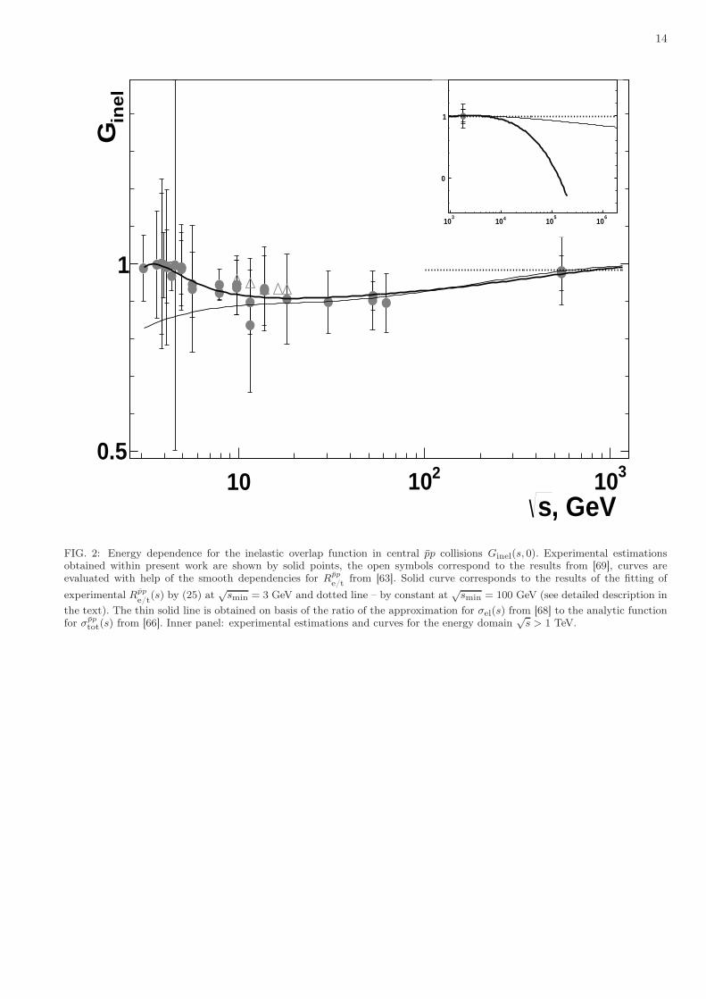
Figs. 1 and 2 show the energy dependence for the inelastic overlap function in central pp and pp collisions,respectively. Estimations for Ginel(s, 0), deduced with the help of the experimental values for Re/t(s) within presentwork, are shown by points. Solid triangles in Fig. 1 are from [69, 70], results for Ginel(s, 0) obtained for pp in [69]are shown by open symbols in Fig. 2. Smooth curves obtained in [63] are also re-calculated for Ginel(s, 0). As seen,estimations for Ginel(s, 0) deduced with the help of the ratio of the elastic to total cross sections, agree quite well withthe results obtained by another techniques in [69, 70] at corresponding

√s for pp (Fig. 1) and pp (Fig. 2) collisions.

1 Below for brevity the joined sample is also called the ensemble for nucleon-nucleon scattering.2 Usually phenomenological models consider the energy domain no wider than

√s & 3− 5 GeV excluding the narrow range on s close to

the low-energy boundary sl.b. ≡ 4m2p for the interactions (pp, pp) under discussion in which Re/t reaches large values in pp, where mp

is the proton mass [66]. Moreover, this low-energy range is excluded in the present analysis due to above condition |ρ(s)| . 0.3.3 In the paper total errors are used for estimations based on the experimental points for Re/t(s), unless otherwise specified. The total

error is calculated as addition of systematic and statistical uncertainties in quadrature [66].

9

Such agreement confirms the validity of the approach used here for the production of the energy dependence of inelasticoverlap function in central pp and pp collisions.

In general, the experimental estimations for Ginel(s, 0) deduced considering the result (22), are featured by largeerrors which turns difficult to obtain unambiguous physical conclusions. Considering large errors, one can supposethat pp (Fig. 1) and pp scattering (Fig. 2) are close to the black disk picture for

√s . 10 GeV. Then, trend is seen for

some decreasing of Ginel(s, 0) up to the highest Intersecting Storage Rings (ISR) energy√s ≈ 63 GeV. There are gaps

without experimental data for both pp and pp, especially large for the first case. The importance of new experimentaldata from Relativistic Heavy Ion Collider (RHIC) at the interval

√s ∼ 0.1 − 0.5 TeV and from low-energy Large

Hadron Collider (LHC) mode for√s ∼ 1.0 TeV is mentioned elsewhere [63]. Experimental estimations for pp for√

s > 1 TeV agree quite well with the black disk picture (Fig. 1, inner panel) and this statement is valid for ppstarting with

√s = 546 GeV (Fig. 2). As seen in Figs. 1, 2, the smooth curves obtained within various models

describe reasonably the experimental estimations for the Ginel(s, 0) in whole available energy range√s ≥ 5 (3) GeV

for pp (pp) collisions. This is expected due to corresponding results for Re/t(s) [63] for the estimations of Ginel(s, 0),deduced within the present work. Moreover, the smooth curves agree reasonably with the estimations obtained byanother technique in [69, 70] for both pp (Fig. 1) and pp (Fig. 2) collisions with some underestimation for the lastcase. The constant Ginel(s, 0) ≈ 1.0 agrees with high-energy pp and pp experimental estimations. Empirical curvebased on (25) is close to the one obtained with parameterizations from [66, 68] for

√s ≤ 1 TeV for both pp (Fig. 1)

and pp (Fig. 2) collisions. In the last case some discrepancy is seen for√s . 10 GeV, which can be explained by the

fact that, strictly speaking, the parametrization for σel from [68] is obtained for√s ≥ 10 GeV. For the pp scattering

both curves based on the result (25) and on the parameterizations from [66, 68] show a gradual decreasing of theGinel(s, 0) considering ultra-high energies

√s & 100 TeV and (25) leading to the noticeable deviation from black disk

limit at O(100 TeV). In general, this observation is also valid for pp (Fig. 2). However, in this case the behavior ofthe curves is characterized by considerable uncertainty in multi-TeV energy domain

√s > 10 TeV due to the lack of

experimental estimations.Fig. 3 shows the Ginel(s, 0) for nucleon-nucleon collisions. Based on the above discussion, the present results are

only shown in Fig. 3 for clearer picture. The experimental estimations agree for pp and pp scattering for close√s.

The constant describe points reasonably for intermediate energies 10 ≤ √s ≤ 100 GeV and for high-energy domain.

One can note that the constant dotted line obtained with the help of the corresponding result for√s > 1 TeV from

[63] agree quite well with experimental estimation at smaller√s = 546 GeV. Then, one can suggest that the constant

allow a reasonable description of the experimental estimations for Ginel(s, 0) for joined nucleon-nucleon sample inwider energy range

√s > 100 GeV with respect to the result for Re/t(s) [63]. The approach based on the (25) predicts

the onset of deviation from the black disk limit at O(100 TeV) and the continues decreasing of the inelastic overlapfunction in central nucleon-nucleon collisions with the growth of s provides Ginel(s, 0) → 0 for PeV energies.

At present the Tsallis statistics is mostly used for successful description of the single-particle transverse momentumdistribution [55–58, 71–75] in various hadron and nucleus collisions in wide energy range. On the other hand, theinformation is very limited regarding the entropy ST and its dependence on some kinematic parameters. In this paper,the estimations are obtained for ST in the impact parameter space and the energy dependence is studied for centralpp, pp collisions.

Taking into account the analysis in [16] the TE in central pp, pp collisions is calculated at√sc = 25.0 GeV in the

present work. As seen from (24), the ζ(s) = 1.0 corresponds to a maximum (s < sc) or a minimum (s > sc) of theST (s, 0). Results from [63] show the ζ(s) ≈ 1.0 can be reached in separate points at intermediate energies

√s ≃ 5

GeV, and this is a characteristic value in TeV energy domain. A detailed analysis of (24) show that ST (s, 0) presentsa sharper behavior as s approaches to the critical value sc. Furthermore, the absolute values of the TE for s < sc(|ST | = −ST ) are mostly larger by orders than that for s ≫ sc (|ST | = ST ) at

√sc = 25.0 GeV. Therefore, the

|ST (s, 0)| seems a more adequate quantity for the study of s-dependence in wide energy domain for the symmetricform of the TE in central pp, pp collisions.

Figs. 4 – 6 show the energy dependence of the magnitude of the TE in central pp, pp collisions and for joinedsample in nucleon-nucleon scattering, respectively. Experimental estimations for |ST (s, 0)| are deduced with help ofthe database for Re/t(s) from [63] and relations (19), (24). Notations for experimental estimations and smooth curvesare the same as in Figs. 1 – 3. Maximum value |ST (s, 0)| ∼ 1 is reached for experimental estimations obtained for ppcollisions close to the critical energy

√sc (Fig. 4), different collisions are featured by similar values of |ST (s, 0)| at close

values of collision energy (Fig. 6) and growth of s leads to the fast decreasing of |ST (s, 0)| for s > sc. The empiricalcurves based on (25) and on the parameterizations from [66, 68] demonstrate the sharp deeps for TeV energies andthese deeps are at various s in pp (Fig. 4) while they coincide in pp scattering (Fig. 5). The parameterizations from[66, 68] provides |ST (s, 0)| mostly large than the empirical function (25) at low and intermediate energies s < sc forboth pp and pp collisions. The situation is more ambiguous at high energies

√s > 1 TeV. For the first case (Fig.

4), the curve evaluated from (25) lies higher than the curve based on the parameterizations from [66, 68] up to the√s ≃ 5 TeV and in the ultra-high energy domain

√s & 100 TeV. In pp scattering (Fig. 5), the fit result from [63]

10

provides smooth curve for |ST (s, 0)|, which is higher than the similar curve deduced with the help of the functionsfrom [66, 68], and difference is especially visible for

√s ≥ 10 TeV.

V. FINAL REMARKS

As pointed out in [16], the total cross section experimental dataset for pp and pp present two fractal dimensions.The Peres–Shmerkin theorem [76] states that if a dataset possesses two fractal dimensions, then the sum of both isnot equal to the original dimension of the dataset [17]. The fundamental question is if the total cross section formsa closed, has no isolated points, dense and compact dataset. Of course, the dataset is dense since the general beliefis that it can be described by a continuous real-valued function of s, for instance. It is compact and has no isolatedpoint as well. However, the term closed implies the existence of a maximum value for the total cross section rise.Note that the Froissart–Martin bound does not prevent this behavior but one cannot assume this from the approachused here.

As noted in [39–41] the region near the central collision (b = 0 fm) presents a growing gray area indicating atendency for higher energies, corroborated by [62, 77]. Moreover, the inelastic overlap function is well-described onlyby the use of at least two Gaussian [62]. This behavior on the impact parameter space may be viewed as a reflex ofthe occurrence of fractal dimensions in energy and momentum spaces [16, 17, 21–26]. Therefore, the inelastic overlapfunction may also present a fractal behavior at each s considered, indicating a phase transition occurring at someb0 = b(sc).

The principle of maximum entropy states that the probability function correctly describing a dataset is the one withthe largest entropy S. The entropy (12) is about a particular scattering at some fixed-s. To each si one can constructa dataset taking the pair

[

0, Ginel(si, b(si))]

, i.e. the line contained in [0, b(si)]. The dataset thus constructed is ahomeomorphism to the Cantor set and then, the Peres–Shmerkin theorem is valid since the dataset formed possesstwo fractal dimensions. Therefore, by the approach used here the precise knowledge of whole Ginel(s, b) is avoided bythe Peres–Shmerkin theorem and the black disk limit may be reduced to a quasi-black disk limit near b = 0 (the graydisk in [39, 40]). This result is independent of the total cross-section reach or not a maximum value.

The TE (12) can also be related to the amount of information in the area of width k−1 and the curve given by m[

1−nGinel(s, b)

]

depending on each s used. Of course, m[

1− nGinel(s, b)]

is limited to the range ∀ i :[

0, Ginel(si, b(si))]

,and, therefore, this area assumes a finite value as well as the amount of information one can obtain from it.

The study of the transition point (the critical temperature) can reveal some important properties of the arrangementof the internal constituents [78]. The temperature at the transition point sc is, of course, of great interest and theresult can easily be obtained by using the Helmholtz free energy. The approach considered here entails the possibilityof negative temperatures occurring inside the hadron in both energy regimes s < sc and s > sc. In the first case,the negative temperature allows to hadron the formation of a torus with a smoothed edge toward the center. Thelatter, indicate the hadron acquires a disk-like shape, tending to a point-like object as the energy tends to infinity. Aswell-known, the negative temperature has been interpreted as the change in the occupancy of the energy states [11]along the years: the probability of the occupation of the higher-energy states is greater than the lower-energy states.Therefore, the phase transition obtained here is evidenced by an inversion of the occupation number of the energystates by the internal constituents of the hadron as the energy increases. The negative temperature also avoids theinternal constituents to gain kinetic energy, turning the system stable [79].

The role of the general entropic index w = (s/sc)α in the present model can be enlarged in the Regge theory context.

As well-known, in this theory, it is expected that scattering amplitude is dominated by the highest trajectory, (s/sc)α,

where α is momentum-transferred dependent. Of course, the α parameter can be written in b-space and, therefore, theTsallis entropy shows a clear connection with the scattering amplitude in the impact parameter space. Moreover, thecuts in the J plane representing the particle exchange can be studied in terms of the Tsallis entropy simply adoptingthe general entropic index. Then, the particle exchange contribution to the Tsallis entropy can be taken into accountin Regge theory. This study will be performed elsewhere.

The phenomenological analysis for the inelastic overlap function and for the magnitude of the TE in central collisionsallows the following conclusions. The Ginel(s, 0) is close to the black disk limit for

√s . 5 GeV and, especially, for

TeV energies in both pp and pp collisions. There is indication on the Ginel(s, 0) < 1 within large errors in the region10 .

√s . 100 GeV. Smooth curves evaluated with the help of the model-independent empirical function (25) and

from parameterizations with universal ln2 ε asymptotic term for σtot, σel show the deviation of Ginel(s, 0) from theblack disk limit for ultra-high energies. The curve based on the model-independent approach predicts Ginel(s, 0) → 0in nucleon-nucleon collisions for PeV energies. The experimental estimations for TE magnitude reaches the maximum|ST (s, 0)| ∼ 1 close to the critical energy and smooth curves predict very small values of |ST (s, 0)| for nucleon-nucleon collisions for ultra-high energies, in particular, |ST (s, 0)| ∼ 10−10 at

√s ∼ 1 PeV in accordance with the

model-independent curve based on the equation (25).

11

Acknowledgments

S.D.C. and C.V.M. thanks to UFSCar by the financial support. The work of V.A.O. was supported partly byNRNU MEPhI Academic Excellence Project (contract No 02.a03.21.0005 on 27.08.2013).

[1] S. Sachdev, Quantum Phase Transitions. Cambridge Univ. Press (2011).[2] M. E. Fisher, Rep. Prog. Phys. 30, 615 (1967).[3] L. D. Landau and E. M. Lifshitz, Statistical physics. Part 1. Elsevier (1980).[4] V. L. Berezinskii, Sov. Phys. JETP 32, 493 (1971).[5] J. M. Kosterlitz and D. J. Thouless, J. Phys. C6, 1181 (1973).[6] C. Tsallis, J. Stat. Phys. 52, 479 (1988); Introduction to Nonextensive Statistical Mechanics: Approaching a Complex

World. Springer (2009).[7] C. E. Shannon, Bell S. Tech. J. 27, 379 (1948).[8] A. Rényi, Proceedings of the IV Berkeley Symposium on Mathematics, Statistics and Probability, p. 547 (1960).[9] I. Bengtsson and K. Zyczkowski, Geometry of Quantum States: An Introduction to Quantum Entanglement. Cambridge

Univ. Press (2006).[10] C. Beck, arXiv: 0902.1235v2 [cond-mat.stat-mech] (2009).[11] L. del Rio et al., Nature 474, 61 (2011).[12] H. Foroozand and S. V. Weijs, Entropy 19, 520 (2017).[13] E. Jiménez, N. Recalde, and E. J. Chacón, Entropy 19, 293 (2017).[14] I. Zborovský and M. V. Tokarev, Int. J. Mod. Phys. A24, 1417 (2009).[15] I. V. Vancea, Int. J. Mod. Phys. A23, 4485 (2008).[16] F. S. Borcsik and S. D. Campos, Mod. Phys. Lett. A31, 1650066 (2016).[17] V. A. Okorokov and S. D. Campos, Int. J. Mod. Phys. A32, 1750175 (2017).[18] A. Bialas and R. Peschanski, Nucl. Phys. B273, 703 (1986).[19] A. Bialas and R. Peschanki, Nucl. Phys. B308, 857 (1988).[20] R. C. Hwa, Phys. Rev. D4

¯1, 1456 (1990).

[21] A. Bialas, Nucl. Phys. A545, 285c (1992).[22] A. Bialas, Acta Phys. Polon. B23, 561 (1992).[23] N. G. Antoniou, F. Diakonos and C. G. Papadopoulos, Phys. Lett. B265, 399 (1991).[24] N. G. Antoniou, V. E. Zambetakis, F. K. Diakonos, and N. K. Diakonou, Z. Phys. C55, 631 (1992).[25] N. G. Antoniou, F. Diakonos, I. S. Mistakidis, and C. G. Papadopoulos, Phys. Rev. D49, 5789 (1994).[26] N. G. Antoniou, N. Davis, and F. K. Diakonos, Phys. Rev. C93, 014908 (2015).[27] A. Deppman, Phys. Rev. D93, 054001 (2016).[28] I. Zborovsk and M. V. Tokarev, Phys. Rev. D75, 094008 (2007).[29] G. Wilk and Z. Włodarczyk, Phys. Lett. B727, 163 (2013).[30] G. Altarelli and G. Parisi, Nucl. Phys. B126, 298 (1977).[31] A. Deppman, T. Frederico, E. Megías, and D. P. Menezes. Entropy 20, 633 (2018).[32] A. Deppman, Adv. High. Ener. Phys.2018, 9141249 (2018)[33] L. Van Hove, Rev. Mod. Phys. 36, 655 (1964).[34] P. D. B. Collins, An Introduction to Regge Theory and High Energy Physics. Cambridge Univ. Press (1977).[35] V. Barone and E. Predazzi, High-Energy Particle Diffraction. Springer (2002).[36] S. D. Campos, Int. J. Mod. Phys. A25, 1937 (2010).[37] N. A. Amos et al. (E710 Collaboration), Phys. Lett. B247, 127 (1990); F. Abe et al. (CDF Collaboration), Phys. Rev.

D50, 5518 (1994).[38] G. Antchev et al. (TOTEM Collaboration), Europhys. Lett. 96, 21002 (2011).[39] I. M. Dremin, Phys. Uspekhi 58, 61 (2015).[40] I. M. Dremin, Phys. Uspekhi 60, 333 (2017).[41] W. Broniowski and E. Ruiz Arriola, Acta Phys. Polon. B Proc. Supp., 10, 1203 (2017).[42] A. Alkin, E. Martinov, O. Kovalenko, and S. M. Troshin, Phys. Rev. D89, 091501 (2014).[43] V. V. Anisovich, V. A. Nikonov, and J. Nyiri, Phys. Rev. D90, 074005 (2014).[44] S. M. Troshin and N. E. Tyurin, Int. J. Mod. Phys. A29, 1450151 (2014).[45] V. V. Anisovich, Phys. Uspekhi 58, 1043 (2015).[46] S. N. Troshin and N. E. Tyurin, Mod. Phys. Lett. A31, 1650079 (2016).[47] J. L. Albacete and A. Soto-Ontoso, Phys. Lett. B770, 149 (2017).[48] E. Ruiz Arriola and W. Broniowski, Phys. Rev. D95, 074030 (2017).[49] R. F. Avila, S. D. Campos, M. J. Menon, and J. Montanha, Eur. Phys. J. C47, 171 (2006).[50] F. S. Navarra, O. V. Utyuzh, G. Wilk, and Z. Wlodarczyk, Phys. Rev. D67, 114002 (2003).[51] P. Jizba and J. Korbel, Phys. Rev. Lett. 122, 120601 (2019).[52] V. Čápek and D. P. Sheehan Challenges to the Second Law of Thermodynamics: Theory and Experiment. Springer (2005).

12

[53] H. Cheng and T. T. Wu, Phys. Rev. Lett. 24, 145 (1970).[54] W. Heisenberg, Z. Phys. 133, 65 (1952).[55] J. Cleymans et al., Phys. Lett. B723, 351 (2013).[56] M. Rybczynski and Z. Wlodarczyk, Eur. Phys. J. C74, 2785 (2014).[57] H. Zheng and L. Zhu, Adv. High Energy Phys. 2016, 9632126 (2016).[58] A.S. Parvan, O.V. Teryaev and J. Cleymans, Eur. Phys. J. A53, 102 (2017).[59] G. Rotundo and M. Ausloos, Eur. Phys. J. B86, 169 (2013).[60] R. Hagedorn, Nuovo Cim. Suppl. 3, 147 (1965); Nuovo Cim. A56, 1027 (1968).[61] I. M. Dremin, Bull. Lebedev Phys. Inst. 44, 94 (2017).[62] D. A. Fagundes, M. J. Menon and P. V. R. G. Silva, Nucl. Phys. A946, 194 (2016).[63] V. A. Okorokov, arXiv: 1805.10514 [hep-ph] (2018).[64] V. V. Anisovich, Phys. Uspekhi, 58, 963 (2015).[65] A. Martin, Phys. Rev. D80, 065013 (2009).[66] M. Tanabashi et al. (Particle Data Group), Phys. Rev. D 98, 030001 (2018).[67] A. Martin and S. M. Roy, Phys. Rev. D91, 076006 (2015).[68] G. Antchev et al. (TOTEM Collaboration), arXiv: 1712.06153 [hep-ex] (2017).[69] D. S. Ayres et al. Phys. Rev. D14, 3092 (1976).[70] U. Amaldi and K.R. Schubert, Nucl. Phys. B166, 301 (1980).[71] J. Cleymans and D. Worku, Eur. Phys. J. A48, 160 (2012).[72] H. Zheng and L. Zhu, Adv. High Ener. Phys. 2015, 180491 (2015).[73] L. Marques, J. Cleymans, and A. Deppman, Phys. Rev. D91, 054025 (2015).[74] H. Zheng, L. Zhu, and A. Bonasera, Phys. Rev. D92, 074009 (2015).[75] Y.–Q. Gao and F.–H. Liu, Indian J. Phys. 90, 319 (2016).[76] Y. Peres and P. Shmerkin, Erg. Theor. Dynam. Syst. 29, 201 (2009).[77] A. K. Kohara, E. Ferreira, and T. Kodama, Eur. Phys. J. C74, 3175 (2014).[78] J. I. Kapusta and K. A. Olive, Nucl. Phys. A408, 478 (1983).[79] S. Braun et al., Science 339, 52 (2013).

13

10 210 3100

0.2

0.4

0.6

0.8

1

1.2

, GeV s10 210 310

in

el

G

0.8

1

1.2

310

410

510

610

1−

0.5−

0

0.5

1

1.5

2

2.5

310 410

510

610

0

2

FIG. 1: Energy dependence for the inelastic overlap function in central pp collisions Ginel(s, 0). Experimental estimationsobtained within present work are shown by open points, the solid symbols correspond to the results from [69, 70], curves areevaluated with help of the smooth dependencies for R

pp

e/tfrom [63]. Solid curve corresponds to the results of the fitting of

experimental Rpp

e/t(s) by (25) at

√smin = 5 GeV and dotted line – by constant at

√smin = 100 GeV (see detailed description in

the text). The thin solid line is obtained on basis of the ratio of the approximation for σel(s) from [68] to the analytic functionfor σ

pp

tot(s) from [66]. Inner panel: experimental estimations and curves for the energy domain√s > 1 TeV.

14

10 210 3100

0.2

0.4

0.6

0.8

1

1.2

1.4

, GeV s10 210 310

in

el

G

0.5

1

310

410

510

610

0

0.2

0.4

0.6

0.8

1

1.2

310 410

510

610

0

1

FIG. 2: Energy dependence for the inelastic overlap function in central pp collisions Ginel(s, 0). Experimental estimationsobtained within present work are shown by solid points, the open symbols correspond to the results from [69], curves areevaluated with help of the smooth dependencies for R

pp

e/tfrom [63]. Solid curve corresponds to the results of the fitting of

experimental Rpp

e/t(s) by (25) at

√smin = 3 GeV and dotted line – by constant at

√smin = 100 GeV (see detailed description in

the text). The thin solid line is obtained on basis of the ratio of the approximation for σel(s) from [68] to the analytic functionfor σ

pp

tot(s) from [66]. Inner panel: experimental estimations and curves for the energy domain√s > 1 TeV.

15

10 210 3100

0.2

0.4

0.6

0.8

1

1.2

1.4

, GeV s10 210 310

in

el

G

0.5

1

310

410

510

610

1−

0.5−

0

0.5

1

1.5

2

2.5

310 410

510

610

0

2

FIG. 3: Energy dependence for the inelastic overlap function in central nucleon-nucleon collisions Ginel(s, 0). Experimentalestimations obtained within present work are shown by open points for pp and by solid points for pp scattering, curves areevaluated with help of the smooth dependencies for Re/t from [63]. Solid curve corresponds to the results of the fitting ofexperimental sample for Re/t(s) joined for pp and pp by (25) at

√smin = 3 GeV, dotted line – by constant at

√smin = 1 TeV,

thin solid curve corresponds the fit of Re/t by constant in the intermediate energy range at√s ∈ [10; 100] GeV (see detailed

description in the text). Inner panel: experimental estimations and curves for the energy domain√s > 1 TeV.

16

10 210 310

3−10

2−10

1−10

1

, GeV s10 210 310

|

T|S

5−10

3−10

1−10

10

310 410

510

610

9−10

8−10

7−10

310 410

510

610

10−10

9−10

8−10

7−10

6−10

FIG. 4: Energy dependence for absolute values of the TE in central pp collisions ST (s, 0). Notations for experimental estimationsand curves are the same as in Fig. 1. Inner panel: experimental estimations and curves for the energy domain

√s > 1 TeV.

17

10 210 310

3−10

2−10

1−10

, GeV s10 210 310

|

T|S

5−10

3−10

1−10

10

310 410

510

610

8−10

7−10

6−10

310 410

510

610

10−10

9−10

8−10

7−10

6−10

FIG. 5: Energy dependence for absolute values of the TE in central pp collisions ST (s, 0). Notations for experimental estimationsand curves are the same as in Fig. 2. Inner panel: experimental estimations and curves for the energy domain

√s > 1 TeV.

18

10 210 310

3−10

2−10

1−10

1

, GeV s10 210 310

|

T|S

5−10

3−10

1−10

10

310 410

510

610

8−10

7−10

6−10

310 410

510

610

10−10

9−10

8−10

7−10

6−10

FIG. 6: Energy dependence for absolute values of the TE in central pp collisions ST (s, 0). Notations for experimental estimationsand curves are the same as in Fig. 3. Inner panel: experimental estimations and curves for the energy domain

√s > 1 TeV.