power system security analysis: applications for wind...
TRANSCRIPT

Power System Security Analysis: Applications for Wind
Power Allocations and Smart Islanding Master of Science Thesis in Electric Power Engineering
Peng Hou
Department of Energy and environment
Division of Electric Power Engineering
CHALMERS UNIVERSITY OF TECHNOLOGY
Göteborg, Sweden, 2010

Page ii
Power System Security Analysis: Applications for Wind
Power Allocations and Smart Islanding
by
Peng Hou
Supervisor: Dr.Tuan A. Le
Examiner: Dr.Tuan A. Le
Master Thesis in ELECTRIC POWER ENGINEERING
Department of Energy and Environment
Division of Electric Power Engineering
Chalmers University of Technology
SE-412 96 Göteborg, Sweden

Page iii
Power System Security Analysis: Applications for Wind Power Allocations and Smart Islanding
© PENG HOU, 2010
Department of Energy and Environment
Division of Electric Power Engineering
Chalmers University of Technology
SE-412 96 Göteborg, Sweden
Telephone + 46 (0)70 040 2179
Chalmers Reproservice
Göteborg, Sweden 2010

Page iv
„„The key to success is
persistence‟‟
To all people I love

Page v
Acknowledgements
This work has been carried out at the Division of Electric Power Engineering, Department
of Energy and Environment at Chalmers University of Technology.
First of all, I would like to express my deep and sincere gratitude to my supervisor and
examiner Dr. Tuan A. Le for his excellent supervision during the work as well as giving the
opportunity for me to explore in depth the area of self-healing of smart grid.
I really appreciate my classmate Yifan Jia and for providing valuable comments and
suggestions. My gratitude also goes to all the master students in Room 2528 for they provide
a good study circumstance for me to focus on my thesis work. I would like to thank Dr. Bin
Ma for his patience every time I asked questions.
My ultimate gratitude goes to my aunt Yenlin Chou and her husband Jeffry. It is because
of their endless concerns that I can accomplish this work eventually.
Also thanks a lot to those people I met who helped me in different ways without being
aware of that.
Natually, the most heartfelt thanks to my parents, Jianling Hou and Xueping Li to
encourage me every day that I was far away from them.
Page vi
Power System Security Analysis: Applications for Wind
Power Allocations and Smart Islanding
Peng Hou
Department of energy and environment
Division of electric Power Engineering
Chalmers University of Technology
Abstract
Power system reliability is the overall objective in power system design and operation. It
includes two main aspects: adequacy and security. During the last decades, outages and
blackout emerged more and more frequently which affected the normal consumption of
consumers. In order to meet the increase the power system security, a self-healing grid is
needed to monitor and response to the change within the whole network in time. Smart
islanding is considered as an effective way to prevent small outages in the system from
propagating into big blackout.
In this paper, two common methods used to find the islands are introduced and the formation
of islands was conducted by a C++ minimal cutset algorithm based program which was
implemented on the platform of Dev cpp in the simulation part, moreover the proposed
approach was applied to a Nordic 32-bus test system and was used to save the network from
voltage collapse. On the other hand, since the large amounts of sustainable resources are
being widely used by taking into account of the ever-increasing load demand throughout the
world, people are exploring new resources to replace the existing non-renewable resources.
As one of the renewable energy, wind power, draws people‟s attentions more and more.
Renewable resource generation connected to the existing network will incur plenty of
problems which will decrease the power system reliability. The wind energy injection will
probably induce transmission overloaded problem which reduce the power system adequacy.
It is critical to allocate the wind energy optimally. In order to find good locations to set up
large-scale wind power projects, a Weighted Transmission Loading Relief (WTLR) / Equal
Transmission Loading Relief (ETLR) sensitivity was introduced in this work to help find the
positions of injecting the wind power so that the increasingly load demand can be satisfied as
well as reduce the contingency overloads within the system to enhance the power system
reliability.
Keywords: Smart islanding, self-healing grid, power system security, minimal cutset, a
C++ minimal cutset algorithm program, renewable energy, power system reliability,
large-scale wind power projects, WTLR/ETLR sensitivity

Page vii
Table of Contents
Chapter 1 .................................................................................................................................... 1
Introduction ................................................................................................................................ 1
1.1 Self-healing grid: Smart islanding ................................................................................................. 1
1.2 Big wind generation project: One trend of the generation development .................................... 3
1.3 Thesis outline ............................................................................................................................. 5
Chapter 2 .................................................................................................................................... 6
Power System Security and Reliability ...................................................................................... 6
2.1 Power System Security .................................................................................................................. 6
2.1.1 Power system operation security ............................................................................................ 6
2.1.2 Security criteria ...................................................................................................................... 7
2.1.3 System security function ........................................................................................................ 7
2.1.4 On-line security analysis ........................................................................................................ 9
2.2 Power System Reliability ............................................................................................................ 10
2.2.1 The concept of reliability ...................................................................................................... 10
2.2.2 Reliability criteria ................................................................................................................. 11
2.3 Power System Stability ............................................................................................................... 12
2.3.1 Power System Stability Standardization............................................................................... 13
2.3.2 Comparisons of power system stability, security and reliability .......................................... 14
2.4 New technologies for improving system reliability and security ................................................ 14
2.4.1 The improvement of reliability by Smart Grid ..................................................................... 14
2.4.2 The contribution of Distributed Generation (DG) to the system security ........................... 15
Chapter 3 .................................................................................................................................. 17
Optimal allocation of wind power in Transmission grids using sensitivity Method ............... 17
3.1 Introduction ................................................................................................................................. 17
3.1 Measuring network security ........................................................................................................ 18
3.1.1 Aggregate MW Contingency Overload (AMWCO) ............................................................ 18
3.1.2 Weighted Transmission Loading Relief (WTLR) ................................................................ 19
3.2.1 System description.............................................................................................................. 21

Page viii
3.2.2 Optimal allocation of wind power ..................................................................................... 22
3.2.3 Case study ............................................................................................................................. 27
3.3 Conclusions ............................................................................................................................... 33
Chapter 4 .................................................................................................................................. 34
Blackout prevention by controlled system islanding ............................................................... 34
4.1 Introduction ................................................................................................................................. 34
4.2 Blackout prevention using System Islanding .............................................................................. 35
4.2.1 Slow coherency based islanding ........................................................................................... 35
4.2.2 Smart Islanding using minimal cutsets ................................................................................. 36
4.2.3 Comparisons of several methods used in finding islands ..................................................... 37
4.3 Case study.................................................................................................................................. 38
4.3.1 System description............................................................................................................... 38
4.3.2 Modelling of transmission lines and power flow in Powerworld ....................................... 38
4.3.3 Enumeration method implemented by Dev cpp .................................................................. 40
4.3.4 Modified islands‟ model ....................................................................................................... 47
4.3.5 Disconnection from the main grid ...................................................................................... 49
Chapter 5 .................................................................................................................................. 55
Conclusions and future work .................................................................................................... 55
5.1 Conclusions ................................................................................................................................. 55
5.2 Future work ............................................................................................................................... 56
Appendix A .............................................................................................................................. 58
Appendix B .............................................................................................................................. 61
Reference .................................................................................................................................. 66
Reference ........................................................................................................................................... 66

Page ix
List of figures
Figure 1.1: Historical analysis of U.S. outages (1991-2005) ................................................................ 1
Figure 1.2: The wind generation capacity worldwide per year from 2001 to 2010 ............................... 3
Figure 2.1: SCADA system ..................................................................................................................... 8
Figure 2.2: Contingency analysis procedure ........................................................................................... 9
Figure 2.3: On-line security analysis framework ................................................................................. 10
Figure 2.4: The meaning of security in the eyes of electric power system operators ............................ 11
Figure 2.5: Classification of power system stability ............................................................................. 12
Figure 3.1: Source and Sink .................................................................................................................. 19
Figure 3.2: The process for determination of good locations ............................................................... 20
Figure 3.3: Nordic 32-Bus System Single Line Diagram .................................................................... 21
Figure 3.4: Voltage profile of scenario 2010 ....................................................................................... 22
Figure 3.5: Simulation phases .............................................................................................................. 23
Figure 3.6: Visualized Weak elements ................................................................................................. 24
Figure 3.7: Visualization of WTLR sensitivity .................................................................................... 26
Figure 3.8: The voltage contour of scenario 2015 without any active power compensation ................ 28
Figure 3.9: The voltage profile of 2015 after wind injection .............................................................. 30
Figure 3.10: The scenario 2015 with wind energy injected to the wrong location ............................. 32
Figure 4.1: Definition of smart grid ...................................................................................................... 35
Figure 4.2: Lumped π-equivalent model of a transmission line and power flowing through it ........... 38
Figure 4.3: Visualization of voltage profile at the point of blackout.................................................... 41
Figure 4.4: The visualization of system blackout with 1600MW power injection .............................. 42
Figure 4.5: The program flow chat ....................................................................................................... 44
Figure 4.6: The voltage visualization of original scenario ................................................................... 45
Figure 4.7: The island found by a controlled partition program .......................................................... 46
Figure 4.8: Minimal net flow V.S Island‟s sizes .................................................................................. 47
Figure 4.9: The modified formation of islands ..................................................................................... 48
Figure 4.10: The contour of voltage profile after the formation of island ............................................ 50
Figure A.1: Scenario 2020 before injecting wind energy ..................................................................... 58
Figure A.2: Scenario 2020 after injecting wind energy ........................................................................ 59
Page x
List of tables
Table 2.1: Power system Stability Requirements .................................................................................. 13
Table 3.1: Weak elements selected by AMWCO ................................................................................ 24
Table 3.2: WTLE&ETLR sensitivity ................................................................................................... 25
Table 3.3: WTLR/ETLR sensitivities of selected buses........................................................................ 29
Table 3.4: Comparisons of differenrt scenarios ................................................................................... 31
Table 3.5: Injection locations and amounts .......................................................................................... 31
Table 4.1 Smart islanding methods comparison .................................................................................. 37
Table 4.2 Islands‟ groups .................................................................................................................... 49
Table A.1: Voltage profile of test system for 2010 .............................................................................. 59
Table A.2: Voltage profile of test system for 2015 .............................................................................. 60
Table A.3: Voltage profile of test system for 2020 .............................................................................. 60
Table B.1: Weak elements selected by AMWCO of scenario 2015...................................................... 61
Table B.2: WTLR&ETLR sensitivity of scenario 2015 ........................................................................ 61
Table B.3: Weak elements selected by AMWCO of scenario 2020...................................................... 62
Table B.4 : WTLR&ETLR sensitivity of scenario 2020 ...................................................................... 62
Table B.5: Final result for islands generated by Dev cpp .................................................................... 63
Table B.6: Line flow created by Powerworld ...................................................................................... 64

Page xi
List of Terms
Acronyms:
NERC North American Electric Reliability Council
EPRI Electric Power Research Institute
OPF Optimal Power Flow
WWEA World Wind Energy Association
TLR Transmission Loading Relief
WTLR Weighted Transmission Loading Relief
ETLR Equal Transmission Loading Relief
SCADA Supervisory Control and Data Acquisition system
HMI Human–Machine Interface
MTU Master Terminal Unit
RTU Remote Terminal Unit
DG Distributed Generation
APCO Average Percentage Contingency Overload
AMWCO Aggregate MW Contingency Overload (AMWCO)
SC Synchronous Condenser
MCs Minimal Cutsets
DAG Directed Acyclic Graph
SS System Splitting
BP Balanced Partition
Voltage Magnitude
Power Factor
Net active power injected at bus i
Net reactive power injected at bus i,
Real part of the element in the line admittance between bus i and j,
Imaginary part of the element in the line admittance between bus i and

Page 1
Chapter 1
Introduction
In this chapter, a general description of the emergence of smart grid that meet the increasing
growth rate of load demand and consumer’s requirement is provided. Due to the fact that
outages and blackouts occurred more frequently during the latest years, the need for an
intelligent strategy to control the electricity network is emphasized by more people
throughout the world. In addition, one important issue, optimal allocation of wind energy,
which is related to the connection of renewable resource to the existing network, is
introduced. Finally, the framework of this thesis is pointed out.
1.1 Self-healing grid: Smart islanding
The statistic report from the North American Electric Reliability Council (NERC) and
analyses from the Electric Power Research Institute (EPRI) tell us such a fact that average
outages from 1984 to now have affected approximately 700,000 customers per event
annually. Outages and large blackout occurred more and more frequently than before during
the last 40 year which spotlighted our requirement to realize the complex phenomena related
to power systems and the development of emergency controls and restoration. The statistic of
outages occurred during 2001-2005 in North America can be seen in Figure 1.1[1] :
Figure 1.1: Historical analysis of U.S. outages (1991-2005)
1991-1995 1996-2000 2001-2005
4158
92
6676
140
Number of US power outages affecting≥50,000 customers

Chapter 1 Introduction
Page 2
In the past 30 years, the information and communication technology has undergone
enormous changes, but the aging America network does not keep up with the pace of
technological evaluation. The consumers proposed higher standards for the power supply
requirements than before, national security, various environmental protection policies also
asked for a power grid with higher standard construction and management level [66]. The
2003 Canada-U.S.A blackout is a motivation for the American electric power industry to
decide to create a robust grid which is safe and reliable, cost-effective, clean and
environmentally friendly, transparent and open, that is, the smart grid.
Actually, the situation in America is not particular. The big blackout around the world
in recent years which are explicated in [3] [4] [5] highlight the requirement for such a self-
healing system with the function of adaptive protection which can minimize the impact on the
whole system performance when there is an emergence of contingency. The critical step of
creating a self-healing grid, it‟s to build a processor into each component of a substation. It
means that each component in the network, namely the breaker, switch, transformer, busbar,
so on, needs to be armed with a processor so that the devices can communicate with each
other. Thus, the infrastructure of the system will be changed. The transmission line must be
accompanied with a parallel information line. The information on device parameters and
device status and analog measurements is recorded in the processors. Once such system is
built up, the updated data will be reported to the central control computers immediately
instead of waiting for the database generated by central control personnel. The system will
therefore be more sensitive to the rapid changes within the system. The emergence of smart
grid provides the possibility for the operators to monitor the system and optimize the
mitigation scheme.
In fact, there are a lot of preventive ways can be applied to avoid total voltage collapse.
In smart grid, the self-healing function can be carried out very well by the smart islanding
approach which has the main goal of splitting the whole system into isolated „islands‟ when
there are failures occurred somewhere within the system. After the formation of the „islands‟,
each of which must then be self-sustaining. The components in each island act as independent
agents with the intelligent distribution. It is capable of reorganizing themselves and makes
best use of available local resources to remove the failure that occurs within the network until
they are able to reconnect to the network. A network of local controllers can act as a parallel,
distributed computer, communicating via microwaves, optical cables, or the power lines
themselves, and intelligently limiting their messages to only that information necessary to
achieve global optimization and facilitate recovery after failure [6] .
Generally speaking, smart islanding is a corrective control strategy that separates the
system into self-sustaining islands after contingency. There are two methods that are
commonly used to form the islands, as slow coherency method and minimal cutset method.
The formation of the islands can be beneficial since it can keep the rest system work normally
which prevents the small outages from evolving into big blackout. The emergence of the self-
healing grid changes the present network into a more robust interactive electric network. This
is of great significance for the optimization of allocation of resources as well as increasing the
efficiency and reliability of power system. Besides, some new technologies‟ research and
development, for instance, wind power, solar power, electric vehicles produces a rapid growth
demand for the development of Smart Grid technology. By integrating the smart islanding
method, the present grid can be transformed into an intelligent self-healing system enhance
power system security and reliability [7] [8] [9] .

Chapter 1 Introduction
Page 3
1.2 Big wind generation project: One trend of the generation
development Energy and environment is the impending problem that should be solved for the
survival and development of human beings. Due to the depleting of fossil fuels, people
highlight the use of sustainable resources which push the prosperity of the rapid development
of environment-friendly products. Wind power, to be one of the renewable resources, has
many advantages as no green gas emission, widely distributed and high potential development
which draw people‟s attention more and more. With the scientific and technological progress,
electric power generation technology, especially wind power generation technology, has made
great advances and steps into maturity by and by. This gives us the opportunity to replay the
present generations with the wind generation and connect it into the existing grid
From the year 2009 statistic report of the World Wind Energy Association (WWEA),
we get to know that all wind turbines installed by the end of 2009 worldwide are generating
340 TWh annum which is the total electricity demand of Italy, the seventh largest economy of
the world, and equals to 2 % of global electricity consumption. The trend of the augmentation
of wind generation worldwide can be seen in Fig 1.2 [10] [11] :
Figure 1.2: The wind generation capacity worldwide per year from 2001 to 2010
24,3231,18 35,3
47,6959,02
74,12
93,93
120,9
159,21
203,50
2001 2002 2003 2004 2005 2006 2007 2008 2009 2010
World Total Installed Capacity[GW]
World Total Installed Capacity[GW]

Chapter 1 Introduction
Page 4
Figure 1.2 shows that the increase of wind generation is over 30% per year with the
highest growth-rate in year 2010. In virtue of the rapid development of the world wind
generation, more and more wind farms are being set up to meet the local demand and mitigate
the burden of transmission instead of long line transmission [12] [13] . [13] This results in the
issue of large-scale integration of wind power generation into the present system. To be
different from the small wind generation farm, the large wind farms are usually connected
into the power grid directly. Hence, more requirements are brought out as the transient
stability; recover ability from accidents, frequency and voltage control as well as automatic
dispatch [14] .
New injections would have an impact on the other transmission lines which results in
the problem of contingency overload. As we know, the transmission overload will decrease
the adequacy of the transmission line which is just one important factor for system reliability.
In order to meet the reliability requirement as well as satisfying the increasing load demand
by using wind generation. The integration of wind projects should be planned by
consideration of problems:
1) The determination of locations of the wind project.
2) The size of the wind project and the strength of the wind output across time.
3) The different injections that incur the overloaded branches which is required to be
expanded.
According to the recommendation of North American Electric Reliability Council, the
system should be designed and operated to withstand N-1 and N-2 contingencies namely
indentifying weak transmission branches by simulating forced transmission and generation
outages and develop a metric to assess the weakness of each existing transmission branch. In
order to satisfy these requirements, the Weighted Transmission Loading Relief (WTLR)/
Equal Transmission Loading Relief (ETLR) sensitivity methodology is used to evaluate the
new wind generations‟ effect on the system [15] .The WTLR means 1 MW new injection at
the specific bus will reduce 0.5 MW contingency overload in transmission branches if we get
a WTLR of 0.5 at that bus while the Equal Transmission Loading Relief (ETLR) signifies the
total expected MW contingency overload reduction, in all transmission lines and under all
contingencies, if 1 MW is injected at that prescribed bus. Positive ETLR and WTLR
sensitivities show that new injection will tend to increase overloads and reduce overall system
security and vice verse [16] . The method gives us the insights into the exploration of the
influence of new injections on the whole system. More details of ETLR/WTLR methodology
will be depicted in Chapter 2.
This thesis describes work on finding methods to improve power system security. The
work includes two parts: the optimal connection of wind power in transmission grids using
sensitivity method as well as development of preventive way, namely controlled partition or
called smart islanding method, for power system blackouts. The main goal of this work is
firstly on a simulation of determining the optimal locations of wind generation project.
Several scenarios are set up to show the results. As we know, more generations on buses will
probably incur the contingency overload. The problem was assumed to be solved by using the
WTLR/ETLR sensitivity method. A study case which is based on Nordic 32 test system is

Chapter 1 Introduction
Page 5
presented to demonstrate the availability of the sensitivity methodology under the help of
Powerworld Simulator Software package. Thereafter, more work is done by implementing the
smart islanding approach into the same test system by using the Powerworld software. As a
self-healing grid, smart islanding should be able to prevent the small outages from evolving
into big blackouts and keep the rest part work normally. The method of forming the „islands‟
was demonstrated by a C++ minimal cutset algorithm based program. Finally, a case study of
applying smart islanding to prevent blackout is demonstrated and presented at last by using
Powerworld software as well.
1.3 Thesis outline
Chapter 2 introduces three important concepts related to the power system operation
issues which are power system stability, security and reliability. The power system reliability
includes two aspects: security and adequacy. A reliable system could sometimes be insecure.
In other words, it could be also operated in the emergency state or went to insecure condition
when it is subjected to a certain disturbance and a stable system can also be insecure when we
compared it with another system. The criteria of system reliability and security are enacted by
different organizations according to different situations. It is the standards for the electrical
engineers to design the network which is presented in this chapter. Moreover, the concept of
power system stability and the interconnection among these three concepts are presented at
last.
In Chapter 3, one issue involved in meeting the continuous grow-up of load demand is
introduced. A WTLR/ETLR sensitivity method is utilized to determine the good locations to
set up wind farms which can satisfy the load increase as well as mitigate the contingency
overload. A case study of Nordic 32 system is presented to see the impact of the new injection
on the whole system. Several scenarios are presented to demonstrate the practicability of this
new methodology. In this section, Powerworld Simulator is used to carry out the simulations
and represent the results graphically.
In Chapter 4, several common methods that are used to find the weak connected areas
during the implement of smart islanding are introduced, moreover, a C++ minimal cutset
algorithm based program is presented to show the results and the process of finding the
“islands” along with the codes are explicated as well, what‟s more, a study case of using
smart islanding approach to protect the power system is shown under the help of Powerworld
simulator.
Main conclusions drawn from this work are summarized in Chapter 5 and different
directions of future researches are also given in this Chapter.

Page 6
Chapter 2
Power System Security and Reliability
Power system reliability is the general purpose in the power system design and operation. If
the system is considered to be reliable, it must be secure most of the time while power system
stability belongs to one aspect of power system secure. To be secure, the system have to be
stable, however, more considerations should be done on the preventions of contingencies
which are not included in the stability problems. Thus, it is critical to understand these
concepts and interconnections among them and construct power system correspond to
standards and criteria which are derived from these concepts to enhance the reliability of the
system as well as satisfy the requirement of the customers.
2.1 Power System Security
2.1.1 Power system operation security
With the increasing electric power demand, electric power system are operates closer to
its stability limit [17] , the operation of power system becomes more complicated and will
become less secure. What‟s more, as a result of restructuring, the problem of power system
security has become one overriding factor in the operation of the electric power system in
deregulated power industry [18] . As it is defined in North American Electric Reliability
Corporation (NERC) (1997), the term „Security‟ has the meaning of the ability of the electric
systems to withstand sudden disturbances such as electric short-circuits or unanticipated loss
of system element, without affecting delivering power to the customers [19] . The objective of
security analysis is to enhance the power system‟s ability to run safely and operate
economically. As described in [20] , it relates to robustness of the system to imminent
disturbances and, hence, depends on the system operating condition as well as the contingent
probability of disturbances.
As detailed in [21] [[22] , power system is said to be operated in the normal state if the
following conditions are met:
1. There is a perfect balance between power generation and load demand; consequently,
the load flow equations are satisfied.
2. The frequency is constant throughout the system.

Chapter 2 Power System Security and Reliability
Page 7
3. The bus voltage magnitude is within the prescribed limit, i.e.
4. No power system component is to be overloaded.
In the power system, the equipments are usually protected by automatic devices which
can make the equipments quit the system immediately once it operates out of its limits. The
event maybe followed by a series of further actions that cause other equipments disconnected
from the system. This is what we called cascading failures. If this process of cascading
failures continues, then the system will suffer from blackout which means the whole network
or most part of it may completely collapse. Thus, it is not sufficient to merely maintain a
system in the normal operating state. We need to specify a security for each system to
withstand the disturbance under distinct conditions.
2.1.2 Security criteria
Assuming that we give a set of disturbances to a power system one at a time. If the
system can also operate in the normal operating state, then the system is said to be secure. In
practice, all power systems cannot avoid being affected by unpredictable faults and failures
such as lightning strikes on transmission lines, mechanical failures in power plants, or fires in
substations. In virtue that this nature phenomenon are unavoidable and happens relatively
frequently, all power systems should be designated to withstand them without emergency. In
order to avoid blackouts and wide scale consumer disconnections, the system should be
operated with a sufficient margin which can be explained in terms of two elements: reserve
generation and transmission capacity.
Reserve generation: Leaving enough reserve generation capacity in case of the loss of
a generating unit.
Transmission capacity: Keeping enough transmission capacity to take up the flow that
was flowing on the outage line.
We also need to know that the system is impossible to be 100% secure since a system
which can be against all contingencies is obviously incredible. The fundamental principle
only requires the system to defend against credible contingencies, that are so called „N-1
contingency‟ as well as „N-2 contingency‟. When the system is subjected to disturbance as
losing any one of its N components and continues to operate normally, it is said to be „„N-1
secure‟‟ while the „„N-2 secure‟‟ means no consumer would be disconnected even if two
components were suddenly disconnected [23] . In engineering, the N-1 contingency secure are
usually a metric for the operators to measure the security of the power system.
2.1.3 System security function
Power system security may be divided into three modes, namely [24] :
1. Steady state security which is created under the steady state condition of a power
system.

Chapter 2 Power System Security and Reliability
Page 8
2. Transient security which copes with the transient state of a system when it is subjected
to a disturbance.
3. Dynamic security which concerns the system response of the order of few minutes
In security evaluation, it is recommendable to find an indicator for each mode of
security which can be revealed by various decision standards and the so called security
function is brought out if the indicator is represented by mathematical functions. Usually, the
security function concerns three major aspects and is carried on in an operations center [28] :
1. System monitoring.
2. Contingency analysis.
3. Security-constrained optimal flow.
The continuous updating information on the conditions of the power system is given to
the operators through system monitoring. Based on this, some quantities such as, voltage,
currents, power flows, and the status of electric equipments as circuit breakers, and switches
in every substation in a power system transmission network can be measured and monitored.
In addition, further information on frequency, generator unit outputs and transformer tap
positions can be also gathered and transmitted back to the control center. By account of the
complexity and arduousness of the task, the data will be processed by digital computers and
then be arranged in a database which gives the chance for the operators to display the
information on large display monitors. What‟s more, the computer can also identify the
overload condition or voltage violations by comparing the incoming information with the
given limits and remind the operators of reacting in time. In practice, supervisory control
systems, a system which allow operators to control circuit breakers and disconnect switches
and transformer taps remotely, are always combined with such systems to create an new kind
of systems. This is what we called supervisory control and data acquisition (SCADA)
system. The SCADA system makes the real time monitoring and correction of overloads or
out-of-limit voltages available. A simplified structure of SCADA can be seen in Figure 2.1:
Figure 2.1: SCADA system
Chapter 2 Power System Security and Reliability
Page 9
Commonly, a SCADA system is composed of three types of communication
equipment: human–machine interface (HMI), master terminal unit (MTU), and the remote
terminal unit (RTU). The function of each part is explicated in [25] . More pertinent
information on SCADA is explained at length in [26] [27] .
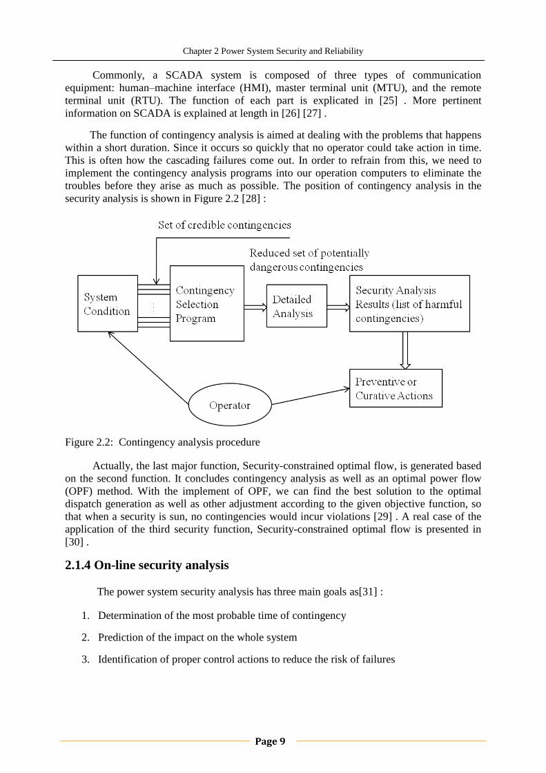
The function of contingency analysis is aimed at dealing with the problems that happens
within a short duration. Since it occurs so quickly that no operator could take action in time.
This is often how the cascading failures come out. In order to refrain from this, we need to
implement the contingency analysis programs into our operation computers to eliminate the
troubles before they arise as much as possible. The position of contingency analysis in the
security analysis is shown in Figure 2.2 [28] :
Figure 2.2: Contingency analysis procedure
Actually, the last major function, Security-constrained optimal flow, is generated based
on the second function. It concludes contingency analysis as well as an optimal power flow
(OPF) method. With the implement of OPF, we can find the best solution to the optimal
dispatch generation as well as other adjustment according to the given objective function, so
that when a security is sun, no contingencies would incur violations [29] . A real case of the
application of the third security function, Security-constrained optimal flow is presented in
[30] .
2.1.4 On-line security analysis
The power system security analysis has three main goals as[31] :
1. Determination of the most probable time of contingency
2. Prediction of the impact on the whole system
3. Identification of proper control actions to reduce the risk of failures
Chapter 2 Power System Security and Reliability
Page 10
In reality, the power system security analysis is usually performed according to N-1
contingency criteria. Some works have already been done on the power system security
analysis technologies as can be known in [32] [33] .
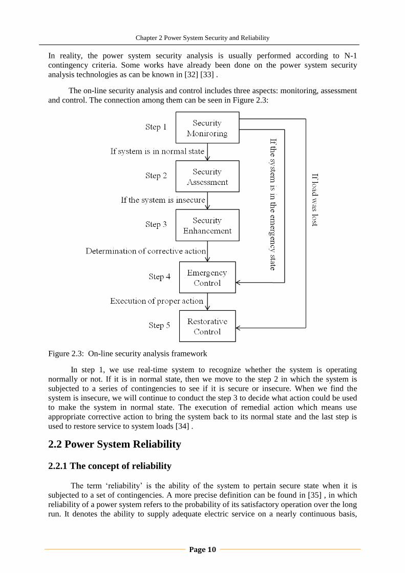
The on-line security analysis and control includes three aspects: monitoring, assessment
and control. The connection among them can be seen in Figure 2.3:
Figure 2.3: On-line security analysis framework
In step 1, we use real-time system to recognize whether the system is operating
normally or not. If it is in normal state, then we move to the step 2 in which the system is
subjected to a series of contingencies to see if it is secure or insecure. When we find the
system is insecure, we will continue to conduct the step 3 to decide what action could be used
to make the system in normal state. The execution of remedial action which means use
appropriate corrective action to bring the system back to its normal state and the last step is
used to restore service to system loads [34] .
2.2 Power System Reliability
2.2.1 The concept of reliability
The term „reliability‟ is the ability of the system to pertain secure state when it is
subjected to a set of contingencies. A more precise definition can be found in [35] , in which
reliability of a power system refers to the probability of its satisfactory operation over the long
run. It denotes the ability to supply adequate electric service on a nearly continuous basis,
Chapter 2 Power System Security and Reliability
Page 11
with few interruptions over an extended time period. According to the definition of NERC,
the reliability is composing of two aspects: security as well as adequacy. On one hand,
adequacy is the ability of systems to supply energy to their customers with satisfying the load
demand. On the other hand, security is the ability of the systems to withstand sudden
disturbances such as short circuit or unanticipated loss of system elements [36] .
In fact, the understanding of the reliability from the operators‟ view is that any
consequence of a credible disturbance that requires a limit. From their eyes, it can also be
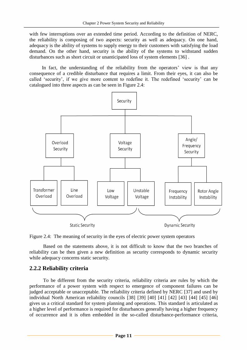
called „security‟, if we give more content to redefine it. The redefined „security‟ can be
catalogued into three aspects as can be seen in Figure 2.4:
Figure 2.4: The meaning of security in the eyes of electric power system operators
Based on the statements above, it is not difficult to know that the two branches of
reliability can be then given a new definition as security corresponds to dynamic security
while adequacy concerns static security.
2.2.2 Reliability criteria
To be different from the security criteria, reliability criteria are rules by which the
performance of a power system with respect to emergence of component failures can be
judged acceptable or unacceptable. The reliability criteria defined by NERC [37] and used by
individual North American reliability councils [38] [39] [40] [41] [42] [43] [44] [45] [46]
gives us a critical standard for system planning and operations. This standard is articulated as
a higher level of performance is required for disturbances generally having a higher frequency
of occurrence and it is often embedded in the so-called disturbance-performance criteria,

Chapter 2 Power System Security and Reliability
Page 12
which specify different classes of allowable performance for different classes of disturbances
[47] .
2.3 Power System Stability
As one aspect of system security, power system stability is the ability of an electric
power system, for a given initial operating condition, to regain a state of operating
equilibrium after being subjected to a physical disturbance, with most system variables
bounded so that practically the entire system remains intact [35] .
According to the physical feature of power system instability, the size of disturbance as
well as by taking into account of time span, process and devices those are included in the
research of power system stability problem. We can divide the power system as three main
types which can be seen in Figure 2.5:
Figure 2.5: Classification of power system stability
The classification of system stability into proper categories is beneficial for us to
indentify critical factors that incur instability and invent philosophies of improving operating
in normal state. Moreover, it contributes to the proper selection and simplification of devices‟

Chapter 2 Power System Security and Reliability
Page 13
models and analysis technologies so that the reasonable operation mode as well as the control
strategy of improving system security level can be arranged scientifically [48] .
2.3.1 Power System Stability Standardization
In [49] , the standardization of steady-state stability requirements and transient stability
requirements are articulated. Based on this, the actual power system stability regulations are
created. The requirements of stability are listed in Table 2.1 as follow [50] :
Table 2.1: Power system Stability Requirements
Normal Design Contingencies Extreme Contingencies
Ι ΙΙ ΙΙΙ
Extreme contingencies
exceeding its severity normal
design contingencies.
Security
Criterion N-1 N-2 N-3 N-k
Acceptable
Consequences
Stable
operation
without
protection
system
intervention
Stable operation with
protection system
intervention
Instability is acceptable.
Power system integrity is
ensured by protection system
and operator intervention.
Normal
Conditions
During design contingencies power system stability must be
maintained for the maximum
permissible transmitted active power
added on random power flow
variations.
The maximum permissible
transmitted active power must
satisfy the standard stead-state
stability margin under normal
conditions
The maximum permissible
transmitted active power must
not exceed the transient stability
limits appropriate to all design
contingencies with due regard to
protection system intervention
During and after extreme
contingencies protection system
and operator intervention must
not lead to cascade outages and
loss of a significant amount of
consumption.

Chapter 2 Power System Security and Reliability
Page 14
Post-fault
Conditions
After design contingencies
Transmitted active power must
satisfy the standard steady-state
stability margin under post-fault
conditions
Transmitted active power must
satisfy the thermal limit
2.3.2 Comparisons of power system stability, security and reliability
Power system stability, security and reliability are three aspects that are widely used to
describe the ability of systems to survive from the unexpected events which can destroy the
equilibrium state of the operation. They are sometimes related to each other, however, there
are still some differences among them [35] :
1. Reliability is the overall objective in power system design and operation. To be
reliable, the power system must be secure most of the time. To be secure, the system
must be stable but must also be secure against other contingencies that would not be
classified as stability problems, for instance, damage to equipment such as an
explosive failure of a cable, fall of transmission towers due to ice loading or sabotage.
As well, a system may be stable following a contingency, yet insecure due to post-
fault system conditions resulting in equipment overloads or voltage violations.
2. System security may be further distinguished from stability in terms of the resulting
consequences. For example, two systems may both be stable with equal stability
margins, but one may be relatively more secure because the consequences of
instability are less severe.
3. Security and stability are time-varying attributes which can be judged by studying the
performance of the power system under a particular set of conditions. Reliability, on
the other hand, is a function of the time-average performance of the power system; it
can only be judged by consideration of the system‟s behavior over an appreciable
period of time.
4. Security and reliability could be considered as the same issue sometimes, however, we
can also distinguish them by adequacy. But we should not overlook such a fact that
even the most reliable systems will not avoid to undertake periods of severe insecurity.
2.4 New technologies for improving system reliability and security
2.4.1 The improvement of reliability by Smart Grid
As has been mentioned in Chapter 1, smart grid is the new product that was generated
in the 20th
century to satisfy the requirement of customers and replace the aging electric grid
gradually. It has many contributions to the increase of the system reliability as [51] :

Chapter 2 Power System Security and Reliability
Page 15
1. Better situational awareness and operator assistance.
2. Autonomous control actions to enhance reliability by increasing resiliency against
component failures and natural disasters, and by eliminating or minimizing frequency
and magnitude of power outages subject to regulatory policies, operating
requirements, equipment limitations and customer preferences. Such control actions
can be more responsive than human operator actions.
3. Efficiency enhancement by maximizing asset utilization
4. Resiliency against malicious attacks by virtue of better physical and IT security
protocols.
5. Integration of renewable resources including solar, wind, and various types of energy
storage. Such integration may occur at any location in the grid ranging from the retail
consumer premises to centralized plants. This will help in addressing environmental
concerns and offer a genuine path toward global sustainability by adopting “green”
technologies including electric transportation.
6. Real-time communication between the consumer and utility so that end-users can
actively participate and tailor their energy consumption based on individual
preferences (price, environmental concerns, etc.).
7. Improved market efficiency through innovative solutions for product types (energy,
ancillary services, risks, etc.) available to market participants of all types and sizes.
8. Higher quality of service–free of voltage sags and spikes as well as other disturbances
and interruptions – to power an increasingly digital economy.
2.4.2 The contribution of Distributed Generation (DG) to the system
security
The distributed generation (DG) is defined by CIGRE(International Coucil on Large
Electric Systems) Working Group 37-23 [52] as a generation not centrally planned by the
utility, not centrally dispatched, normally smaller than 50-100 MW and usually connected to
distribution power systems (networks to which customers are connected, typically ranging
from 230 V/400 V to 145 kV). The increasing demand of DG can be relied on its financial
value which is discussed in [53] .
Presently, there are several renewable resources which are concerned by most of
people as, wind power, cogeneration, photovoltaic (PV), small hydro and waste/biomass.
Those resources can all be considered as DGs. Different forms of DGs have been installed in
Europe and wind energy posses the fastest rates of development with 75GW to be installed in
Europe in 2010 [54] and still keeps the increasing rate of growth in some countries. The
explanation of this phenomenon can be quite comprehensive, however, there is no doubt that
the application of DGs should be due to its economic benefits as well as its contribution to the
system reliability.
As has been articulated in [55] , the large-scale penetration of DG will change the
power flows in the distribution network. The change in real and reactive power flows caused
by DG has its meaning in both technical and economic aspects. Besides, DG can increase the

Chapter 2 Power System Security and Reliability
Page 16
power system security by ensuring a frequency control which can be proved by the case of
wind farms that are asked to contribute to frequency control in Ireland and Denmark. In sum,
the penetration of DGs will contribute to the enhancement of electric grid security and the
development of DG technology is far-reaching.
Page 17
Chapter 3
Optimal Allocation of Wind Power in
Transmission Grids using Sensitivity
Method
The purpose of this chapter is to show how the WTLR/ETLR sensitivity method is used in
determination of optimal allocation of wind power. Firstly, some concepts are introduced,
which include Aggregate MW Contingency Overload (AMWCO), the aggregate percent
contingency overload(APCO), Transmission Loading Relief (TLR ), equivalent TLR (ETLR)
and Weighted Transmission Loading Relief (WTLR), then a case study which is based on
Nordic 32 test system is presented to demonstrate the results. The Powerworld Simulator is
used to set up the model and solve the problems of getting the good locations as well as the
amounts of injection on each location. Finally, several scenarios are studied to see the
practical value of using sensitivity methodology. The models for different scenarios are also
set up by the Powerworld Simulator and the results are obtained based on the method
mentioned above.
3.1 Introduction
Nowadays, two impending problems confine the survival and development of human
beings, namely energy and environment. In virtue of the increasing depletion of fossil fuel
and increasing concerns on the global environment from people all over the world,
governments and international organizations have invested on the exploration of renewable
energy in succession from 70s of last century to dig out a resource and environment
coordinated path which corresponds to the socio-economic progress as well as sustainable
development. As one kind of renewable resources, wind power plays an importance role for
its development potential and outstanding advantages. The wind generation has the most
mature technology, largest development and commercialization prospects which draw
attentions of various countries and results in the widely utilization and exploration throughout
the world [56] .
Under the support from the governments, the research of wind generation undertakes a
great progress. Many countries as Sweden, Germany, Denmark and U.S.A has begun the
projects of large-scale integration of wind generation due to its own advantages of short

Chapter 3 Optimal Allocation of Wind Power in Transmission Grids using Sensitivity Method
Page 18
construction period, flexible installed capability, saving fossil energy, relieving contradictions
in power supply and adjusting the energy structure as well as non-consume of fuel, on-
pollution influence to the surroundings during operation which has a profound function in
maintaining ecological balance.
The work of connecting large-scale wind generation into the power network will
generate several problems, such as voltage deviation, voltage fluctuation, flicker and
harmonics while more studies have to be done before this. The construction of large wind
farms usually come out with the problem of determination of good positions to inject. Where
and how much energy should we inject would be a problem for the current electrical
engineers [57] [58] [59] .
3.1 Measuring network security
3.1.1 Aggregate MW Contingency Overload (AMWCO)
System security always means the network operates without loss of loads, voltage
violations, transmission branches flows within the thermal limits as well as enough safe
margins from the collapse point. The strategy for designating a traditional power system is
usually done by strictly following the criteria which are set up by different organizations.
Usually, the system is designed and planned by taking the N-1 and N-2 contingency analysis
which is according to the recommendation of the NERC. In order to show the severity of
contingencies as well as the emergency of multiple violations, an indicator is introduced, that
is, the aggregate percent contingency overload (APCO) [60] , which can be defined as follow:
APCO is the total percent overload flow shown on a certain transmission line during a
series of contingencies. We also have the interest to define another quantity to change the
overload expression from percentage form into the real value. This is so called Aggregate
megawatt contingency overload (AMWCO) which is expressed as,
From the expression, we can see that the AMWCO is actually calculated by using
MVA rating instead of MW. It is necessary to be in accordance with the definition of
transmissions loading relief (TLR) which will be explained later.
Based on these two quantities, we can easily point out the weak elements1. The higher
the value is, the weaker the transmission element is. While zero means no overload
contingency happens on this line. In spite that both two quantities are able to rank the
weakness, we prefer to use AMWCO in most case since it can give the real value information
[61] .
1 It means when there is contingency on other transmission line this line will undertake serous overloading.
Chapter 3 Optimal Allocation of Wind Power in Transmission Grids using Sensitivity Method
Page 19
3.1.2 Weighted Transmission Loading Relief (WTLR)
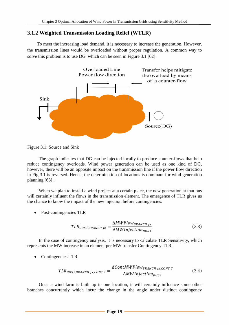
To meet the increasing load demand, it is necessary to increase the generation. However,
the transmission lines would be overloaded without proper regulation. A common way to
solve this problem is to use DG which can be seen in Figure 3.1 [62] :
Figure 3.1: Source and Sink
The graph indicates that DG can be injected locally to produce counter-flows that help
reduce contingency overloads. Wind power generation can be used as one kind of DG,
however, there will be an opposite impact on the transmission line if the power flow direction
in Fig 3.1 is reversed. Hence, the determination of locations is dominant for wind generation
planning [63] .
When we plan to install a wind project at a certain place, the new generation at that bus
will certainly influent the flows in the transmission element. The emergence of TLR gives us
the chance to know the impact of the new injection before contingencies.
Post-contingencies TLR
In the case of contingency analysis, it is necessary to calculate TLR Sensitivity, which
represents the MW increase in an element per MW transfer Contingency TLR.
Contingencies TLR
Once a wind farm is built up in one location, it will certainly influence some other
branches concurrently which incur the change in the angle under distinct contingency
Chapter 3 Optimal Allocation of Wind Power in Transmission Grids using Sensitivity Method
Page 20
conditions. Therefore, an equivalent TLR (ETLR) sensitivity is nominated to catch the entire
variation of flows during contingencies after injection.
Despite that the ETLR remarks the simultaneous effect of Injection, it does not consider
the severity of the contingency overloads which is the base to mitigate overload at times. This
is overcome by WTLR which has the general formation as follow:
: The overload direction, if the line is overloaded in the forward direction during
all the contingencies, then the value will be 1 while the value will be minus 1, if it is always
overloaded in the reverse direction during all contingencies [64] .
: The number of contingencies,
In general, the ETLR and WTLR sensitivity are two good indicators to help decide the
good locations to inject. The ETLR signifies the total expected MW contingency overload
reduction, in all transmission lines and under all contingencies, if 1 MW is injected at that
prescribed bus. Positive ETLR and WTLR sensitivities point that new injection will tend to
increase overloads and reduce overall system security and vice verse. While 1MW of new
injection at the particular bus has a great possibility to reduce 0.5 MW of overload in
transmission branches during contingencies, if a WTLR value of 0.5 is seen at that bus. Based
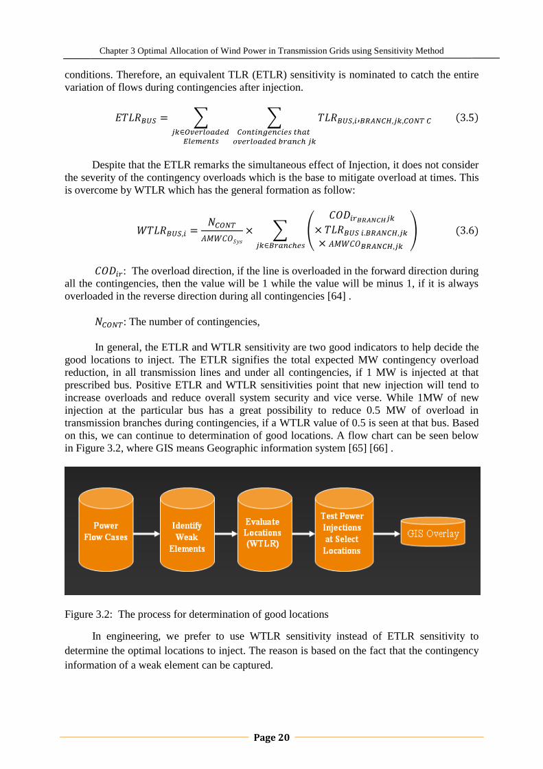
on this, we can continue to determination of good locations. A flow chart can be seen below
in Figure 3.2, where GIS means Geographic information system [65] [66] .
Figure 3.2: The process for determination of good locations
In engineering, we prefer to use WTLR sensitivity instead of ETLR sensitivity to
determine the optimal locations to inject. The reason is based on the fact that the contingency
information of a weak element can be captured.
Chapter 3 Optimal Allocation of Wind Power in Transmission Grids using Sensitivity Method
Page 21
3.2 Simulation part
The previous concepts have been demonstrated using Powerworld Simulator and a
32-bus test system. What more, the ETLR/WTLR methodology is performed in order to
obtain optimal allocation of wind generation.
3.2.1 System description
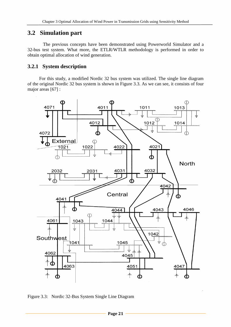
For this study, a modified Nordic 32 bus system was utilized. The single line diagram
of the original Nordic 32 bus system is shown in Figure 3.3. As we can see, it consists of four
major areas [67] :
Figure 3.3: Nordic 32-Bus System Single Line Diagram
Chapter 3 Optimal Allocation of Wind Power in Transmission Grids using Sensitivity Method
Page 22
• External: connected to the North. It has a mix of generation and load.
• North: with basically hydro generation and some load.
• Central: with a large amount of load and rather large thermal power generation.
• Southwest: with a few thermal units and some loads.
The power is basically transferred from the “North” area to the “Central” area. The system
has its main transmission system designed for 400 kV, with some other regional systems at
130kV and 220kV. There are total 19 generators and shunt compensation is considered in case
of voltage violation. Bus 4011 is selected as the slack bus, moreover, Bus 4071 and 4072 is
chosen as the external part which can be regarded as the foreign country power supply.
3.2.2 Optimal allocation of wind power
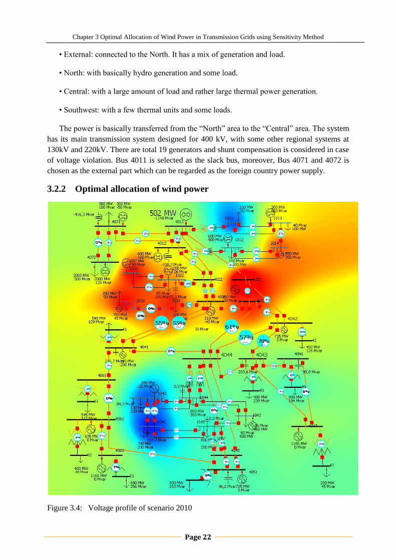
Figure 3.4: Voltage profile of scenario 2010
Chapter 3 Optimal Allocation of Wind Power in Transmission Grids using Sensitivity Method
Page 23
From the base case, we can see that the five main lines which transport power from
north to south are undergoing more loading than the other lines. Hence, we can predict that
there will be overloading problems occurred on these lines when we increase the load
demand. Originally, we have a Nordic 32 test system with a total 10940MW loads demand.
According to the statistic report of Nordel, the electricity consumption in Nordic power
market is assumed to grow 1.5% per year [68] . Based on this, we give a 1.5% load increase
per year to the Nordic 32 test system and increase the load demand to 11785 MW after 5
years load augment and this is considered to be the base case which can be seen in Figure 3.4:
We give the name scenario 2010 to the base case for further use. Also we set up
another two scenarios, namely scenarios 2015 and scenarios 2020 to present the results and
analysis. The creations of these two scenarios are based on the above statement. We give a
1.5% load increase every year and the load demand for scenario 2015 and 2020 are
12696MW and 13678MW respectively. We emphasized the existence of the slack bus
generator and the five main lines because the slack bus generator will support the whole
system once there is load-generation imbalance while the five main lines are undertaking the
highest power transmission burden. The colored background shows the voltage difference
among the system. The red means the highest voltage and blue means the lowest voltage. The
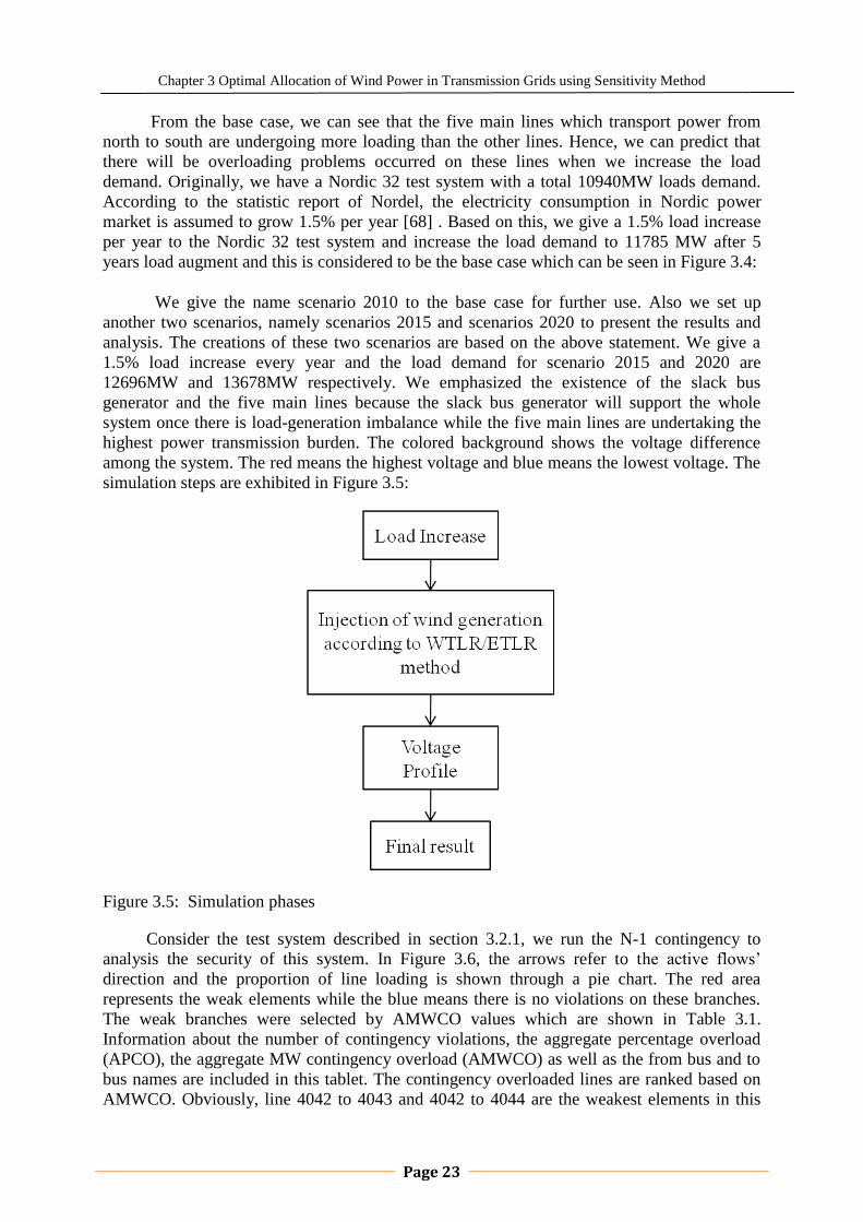
simulation steps are exhibited in Figure 3.5:
Figure 3.5: Simulation phases
Consider the test system described in section 3.2.1, we run the N-1 contingency to
analysis the security of this system. In Figure 3.6, the arrows refer to the active flows‟
direction and the proportion of line loading is shown through a pie chart. The red area
represents the weak elements while the blue means there is no violations on these branches.
The weak branches were selected by AMWCO values which are shown in Table 3.1.
Information about the number of contingency violations, the aggregate percentage overload
(APCO), the aggregate MW contingency overload (AMWCO) as well as the from bus and to
bus names are included in this tablet. The contingency overloaded lines are ranked based on
AMWCO. Obviously, line 4042 to 4043 and 4042 to 4044 are the weakest elements in this
Chapter 3 Optimal Allocation of Wind Power in Transmission Grids using Sensitivity Method
Page 24
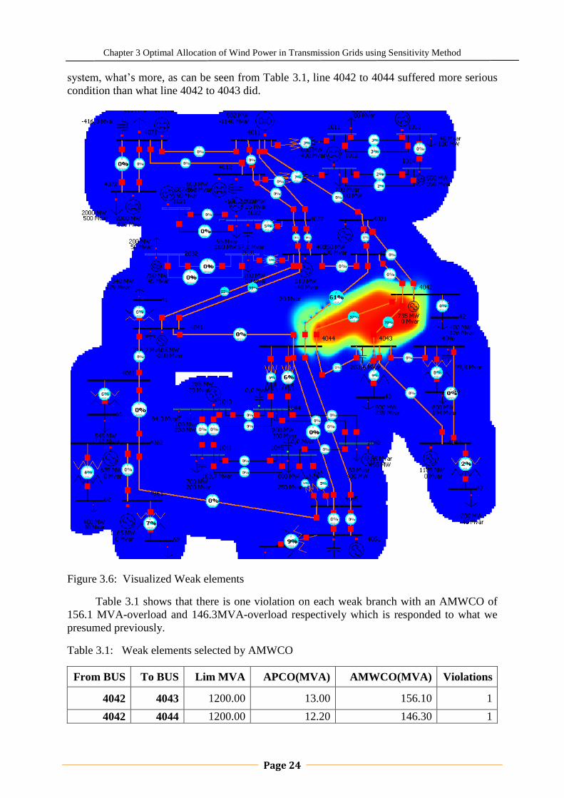
system, what‟s more, as can be seen from Table 3.1, line 4042 to 4044 suffered more serious
condition than what line 4042 to 4043 did.
Figure 3.6: Visualized Weak elements
Table 3.1 shows that there is one violation on each weak branch with an AMWCO of
156.1 MVA-overload and 146.3MVA-overload respectively which is responded to what we
presumed previously.
Table 3.1: Weak elements selected by AMWCO
From BUS To BUS Lim MVA APCO(MVA) AMWCO(MVA) Violations
4042 4043 1200.00 13.00 156.10 1
4042 4044 1200.00 12.20 146.30 1

Chapter 3 Optimal Allocation of Wind Power in Transmission Grids using Sensitivity Method
Page 25
For the purpose of increasing system security, new injection should be located properly
to generate counter-flow in the overloaded branches to help fulfill the mitigation. Therefore,
we need to calculate the ETLR and WTLR sensitivity to go on with the selection work. The
ETLR as well as WTLR results for each branch are listed in Table 3.2:
Table 3.2: WTLE&ETLR sensitivity
Multiple Bus TLR Sensitivities
Number ETLR WTLR 4042 to 4043 4042 to 4044
41 -0.11 -0.11 -0.04 -0.07
42 0.55 0.55 0.26 0.29
43 -0.36 -0.38 -0.38 0.01
46 -0.36 -0.37 -0.38 0.01
47 -0.36 -0.37 -0.37 0.01
51 -0.31 -0.31 -0.13 -0.18
61 -0.17 -0.17 -0.06 -0.10
62 -0.18 -0.18 -0.07 -0.11
63 -0.17 -0.17 -0.07 -0.11
1011 0.12 0.12 0.06 0.06
1012 0.12 0.12 0.07 0.05
1013 0.12 0.12 0.07 0.05
1014 0.12 0.12 0.06 0.05
1021 0.10 0.10 0.06 0.04
1022 0.09 0.09 0.05 0.04
1041 -0.34 -0.33 -0.14 -0.19
1042 -0.29 -0.29 -0.12 -0.17
1043 -0.32 -0.32 -0.14 -0.19
1044 -0.30 -0.30 -0.12 -0.18
1045 -0.30 -0.30 -0.13 -0.18
2031 0.06 0.06 0.04 0.02
2032 0.07 0.07 0.04 0.03
4011 0.12 0.12 0.06 0.06
4012 0.11 0.11 0.06 0.05
4021 0.23 0.23 0.11 0.11
4022 0.09 0.09 0.05 0.04
4031 0.06 0.06 0.04 0.02
4032 0.11 0.11 0.06 0.05
4041 -0.11 -0.11 -0.04 -0.07
4042 0.55 0.55 0.26 0.29
4043 -0.37 -0.38 -0.38 0.01
4044 -0.30 -0.30 -0.12 -0.18
4045 -0.30 -0.30 -0.12 -0.18
4046 -0.37 -0.38 -0.38 0.01
4047 -0.36 -0.38 -0.38 0.01
4051 -0.31 -0.30 -0.13 -0.18
4061 -0.16 -0.16 -0.07 -0.10
4062 -0.18 -0.17 -0.07 -0.11
4063 -0.17 -0.17 -0.06 -0.11
Chapter 3 Optimal Allocation of Wind Power in Transmission Grids using Sensitivity Method
Page 26
4071 0.12 0.12 0.06 0.05
4072 0.12 0.12 0.06 0.05
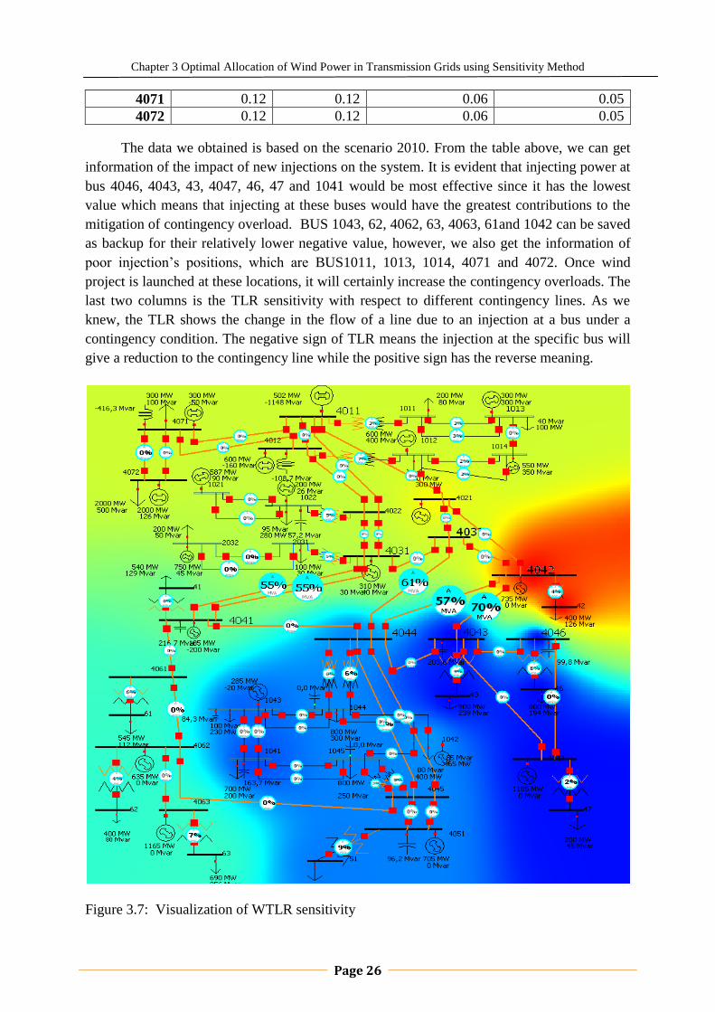
The data we obtained is based on the scenario 2010. From the table above, we can get
information of the impact of new injections on the system. It is evident that injecting power at
bus 4046, 4043, 43, 4047, 46, 47 and 1041 would be most effective since it has the lowest
value which means that injecting at these buses would have the greatest contributions to the
mitigation of contingency overload. BUS 1043, 62, 4062, 63, 4063, 61and 1042 can be saved
as backup for their relatively lower negative value, however, we also get the information of
poor injection‟s positions, which are BUS1011, 1013, 1014, 4071 and 4072. Once wind
project is launched at these locations, it will certainly increase the contingency overloads. The
last two columns is the TLR sensitivity with respect to different contingency lines. As we
knew, the TLR shows the change in the flow of a line due to an injection at a bus under a
contingency condition. The negative sign of TLR means the injection at the specific bus will
give a reduction to the contingency line while the positive sign has the reverse meaning.
Figure 3.7: Visualization of WTLR sensitivity

Chapter 3 Optimal Allocation of Wind Power in Transmission Grids using Sensitivity Method
Page 27
In Figure 3.7, a visualization of the WTLR sensitivity is shown. The blue area indicates
the best locations for new generation while the red zone indicates the poor locations. We also
show interests on some areas which is painted with orange color. This area seems to be
insensitive to the new injection. Injections at these places would have insignificant effect. We
can prove our assumption by looking it up in Table 3.2. In which we can see that the WTLR
sensitivities of these buses are close to zero.
Another conclusion can be drawn by comparing the Figure 3.6 with Figure 3.7,
namely, the positive values of WTLR always come out at the sending end of the weak
branches, and the flipside of this is that negative values are always found at the receiving end.
This has the practical meaning as in a power market, we usually gives a higher price at the
receiving end and a lower price at the sending end in order to call the market participants‟
attentions on generating more at these locations. The simulation result is just in accord with
this strategy [69] .
3.2.3 Case study
According to the report of Nordel, the electricity consumption in Nordic power market
is assumed to grow 1.5% per year. Based on the scenario 2010 which is modified from the
Nordic 32 system with a total load demand of 11785MW which has been described
previously, we simulate the load increase for year 2015 and 2020. We give 1.5% increase
consumption annually and inject wind energy to compensate for the imbalance between load
and generation respectively. Commonly, the load increase problems can be solved by
generation dispatch method. But if the generators in the system has already reached its limits,
that is to say, the generators cannot dispatch more active power any more. In the case of this,
the generators in the system could not change its output to compensate for the load increase
automatically and maintain the generation-load balance if we apply the dispatch generation
method. Thus, some other approach is calling for to handle this issue. As one form of DGs,
wind injection can be selected to meet the requirement. The optimal allocation of wind
injection is conducted by using the WTLR/ETLR sensitivity methodology which will be
presented in the following statement.
In all scenarios, we increase the load on southern part with uniformly amount of
augment. Shunt devices are installed to get a better voltage profile. During the simulation, we
use a Synchronous Condenser (SC) to control the voltage at the beginning and then substitute
it with shunt devices. This is due to the fact that we should not have so many synchronous
condensers in the system in reality, however, shunt devices are usually installed on every
substation for the sake of compensation or absorption. Hence, we use the SC just for the
consideration of finding a more precise value for shunt devices. In Powerworld Simulator, a
SC is generated by setting the active power output to zero in the control panel of generator.
As well, we use a negative load to simulate the effects of wind power injections. The
utilization of negative loads instead of generators is by considerations of its convenience.
Usually, the power factor of wind turbines can be set as 0.85, however, we did not inject any
reactive power in these two scenarios, in other words, our wind turbines are assumed to be
with a 1.0 power factor. This is due to the reason that the WTLR/ETLR sensitivity is actually
active power sensitivity. If we inject the reactive power in each bus, it will influence the
loading of each line and give us the obstacle to analyze the final result.

Chapter 3 Optimal Allocation of Wind Power in Transmission Grids using Sensitivity Method
Page 28
3.2.3.1 Case analysis for scenario 2015
Figure 3.8: The voltage contour of scenario 2015 without any active power compensation
Figure 3.8 shows the condition after load increase without any new injection. It
visualized the voltage distribution of scenario 2015. The red color means the voltage was
already over 1.15 per unit. In order to support the system and compensate for the imbalance
between generation and load, the slack bus generator would support the network by producing
more active power. As can be seen, the active power output of the slack bus generator has
already reached 1610MW which is far away from its limit of 1000MW while the five main
lines which deliver powers from North to south are suffering from high loading contingencies
as well. If there is a disturbance happened somewhere within the system, the system would
collapse. We need a method to increase the security of this system.
Chapter 3 Optimal Allocation of Wind Power in Transmission Grids using Sensitivity Method
Page 29
The pie charts of the five main lines show the loading of the present line. It is the
critical parts to prove our assumption that is the optimal allocation of wind energy will help
mitigate the contingency overload. According to the theory mentioned above, we found the
weak elements at first and then generated the WTLR/ETLR sensitivities by Powerworld
Simulator. The data can be seen in Appendix B, Table B.1 and Table B.2 respectively. The
data in these tables gives us several selections to choose where to inject. It is obviously that
BUS1041, BUS1043 and BUS4051 are the optimal locations. We inject 1200MW power into
these buses uniformly. The amount of injection is selected by consideration of two aspects:
slack bus generator output and loading of five main lines. We intercept part of Table B.2 to
analyze, as follow:
Table 3.3: WTLR/ETLR sensitivities of selected buses
Bus
Name ETLR WTLR
TLR
4031 to
4041
TLR
4031 to
4041
TLR
4032 to
4044
TLR
4042 to
4043
TLR
4042 to
4044
1041 -0.69 -0.78 -0.09 -0.09 -0.19 -0.13 -0.19
4051 -0.67 -0.75 -0.09 -0.09 -0.18 -0.13 -0.18
1043 -0.68 -0.77 -0.09 -0.09 -0.19 -0.13 -0.18
From the theory we mentioned in section 3.1.1, we get to know that a WTLR of 0.5 at a
bus means that 1MW of new generation injected at the specific bus is likely to reduce 0.5
MW of overload in transmission elements during contingencies while a ETLR of 1 represents
the expected MW contingency overload reduction, in all branches and under all contingencies
when we inject 1MW at that particular bus. Based on these, we can draw the conclusion that
the new injection at Bus1041 is likely to reduce 156MW, 0.78 multiply by 400MW and
divided by two, of overload in transmission elements during contingencies while it also
contributes to 276MW, 0.69 multiply by 400MW, contingencies overload reduction.
Moreover, the effects of new injection on line 4031 to 404, 4032 to 404, 4012 to 4043
and 4042 to 4044 can be analyzed by the TLR sensitivities which show the power flow
change of a line due to the new injection at the specific bus. In our case, the injection at
Bus1041 helps mitigate these five lines by a power flow reduction of 36MW, 36MW, 76MW,
52MW and 76MW respectively. The results of influence of the other injections on other lines
can be obtained by similar process. The visualization of voltage profile after wind injection
and the loading information of five main lines in this case can be seen in Figure 3.9:
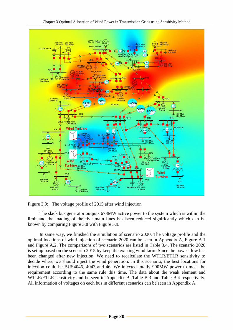
Chapter 3 Optimal Allocation of Wind Power in Transmission Grids using Sensitivity Method
Page 30
Figure 3.9: The voltage profile of 2015 after wind injection
The slack bus generator outputs 673MW active power to the system which is within the
limit and the loading of the five main lines has been reduced significantly which can be
known by comparing Figure 3.8 with Figure 3.9.
In same way, we finished the simulation of scenario 2020. The voltage profile and the
optimal locations of wind injection of scenario 2020 can be seen in Appendix A, Figure A.1
and Figure A.2. The comparisons of two scenarios are listed in Table 3.4. The scenario 2020
is set up based on the scenario 2015 by keep the existing wind farm. Since the power flow has
been changed after new injection. We need to recalculate the WTLR/ETLR sensitivity to
decide where we should inject the wind generation. In this scenario, the best locations for
injection could be BUS4046, 4043 and 46. We injected totally 900MW power to meet the
requirement according to the same rule this time. The data about the weak element and
WTLR/ETLR sensitivity and be seen in Appendix B, Table B.3 and Table B.4 respectively.
All information of voltages on each bus in different scenarios can be seen in Appendix A.

Chapter 3 Optimal Allocation of Wind Power in Transmission Grids using Sensitivity Method
Page 31
3.2.3.2 Comparisons and Discussions
The Voltage Deviation parameter, gives us an idea of how much the bus voltages are
deviated from 1.0 per unit. It was calculated with the following formula:
Where:
: The voltage at bus „i‟ in p.u.
n: The total number of buses
Comparisons of several scenarios
Table 3.4: Comparisons of different scenarios
Test system Scenario 2010 Scenario 2015 Scenario 2020
Consumption(MW) 10940.00 11785.00 12696.00 13678.00
Generation(MW) 11391.80 12226.70 13025.90 13902.20
Compensation(Mvar) 961.23 1107.88 1950.18 2073.22
Absorption(Mvar) 308.65 525.00 1313.77 -1469.94
Wind injection(MW) 0.00 0.00 1200.00 900.00
Voltage deviation 0.18 0.05 0.06 0.06
The result of voltage deviation on load buses is derived from 1.00 per unit standard
voltage parameter, which shows that the voltage condition in each scenario is almost same.
The final results of optimal locations and the amount of power that should be injected at
the selected location for both scenarios is shown in Table 3.5:
Table 3.5: Injection locations and amounts
Scenario Bus Name Injection Amount
2015
1041 400.00
1043 400.00
4051 400.00
2020
4046 300.00
4043 300.00
46 300.00
In summary, it is so apparently that the system is running normally under different
scenarios and all the models show its priority in both voltage stability and system losses in

Chapter 3 Optimal Allocation of Wind Power in Transmission Grids using Sensitivity Method
Page 32
comparison with the base case. Hence, the ETLR/WTLR sensitivity is proved to be a useful
indicator for us to decide the locations to install wind project at that location. What‟s more,
we also injected wind energy at BUS.4042 at which the WTLR/ERLT sensitivities are
positive to demonstrate the theory.
Figure 3.10: The scenario 2015 with wind energy injected to the wrong location
Figure 3.11 shows the result after injecting 800MW active power at BUS4042 at which
the ETLR and WTLR sensitivity are positive. By comparing Figure 3.11 with Figure 3.9 and
Figure 3.8, we notice that the loading of line 4031 to 4041 and line 4032 to 4044 is reduced
while the loading of line 4042 to 4043 and line 4042 to 4044 are increased. The phenomenon
can be explained by looking up the Table B.4. In which we notice that the sign of TLR
sensitivities for the case injecting at Bus 4042 is not consistent. The line 4032 to 4041 and
line 4032 to 4044 has a negative sign which means new injection at Bus 4042 will help
mitigate the overloaded contingency on these two lines and the positive sign can be seen on

Chapter 3 Optimal Allocation of Wind Power in Transmission Grids using Sensitivity Method
Page 33
the other two lines shows that the new injection will change the power flow of the two lines
and worsen the overload contingency.
In general, injection at unsuitable place will increase contingency overload while the
optimal allocation of wind energy can help mitigate the overloaded situation. Different
injections can have different effects on different lines during different contingencies.
3.3 Conclusions
In this section, a methodology to determine the good locations of wind energy is
presented. Different scenarios are proposed and analyzed to understand the effects of new
injections on other branches. The utilization of ETLR/WTLR approach has succeeded in
mitigating the problem of contingency overload induced by load enhancement as well as the
determination of proper location of wind project and amounts of new injection which proves
the practicality of this method. Actually, the reduction of the loading on the contingency lines
means the increase of adequacy which is one aspect of power system reliability. The optimal
allocation of wind energy is a mitigation scheme which reduces the overload contingency.
This action can maintain the power system operate in normal state, that is to say, operate
securely. By using the proposed methodology, the power system security and reliability could
be increased. Finally, synchronous compensators are used to help find a more accurate value
for shunt devices. However, in this case we have a lot of injection points to select instead of
choosing it more scientifically we just choose it according to WTLR/ETLR sensitivity
without taking into account of the economic factors, such as local generation prices as well as
the availability of the wind power. It is a drawback which can be overcame by modifying the
model and constrains in future.
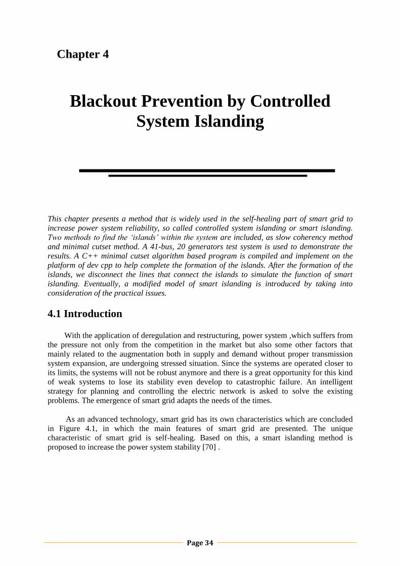
Page 34
Chapter 4
Blackout Prevention by Controlled
System Islanding
This chapter presents a method that is widely used in the self-healing part of smart grid to
increase power system reliability, so called controlled system islanding or smart islanding.
Two methods to find the ‘islands’ within the system are included, as slow coherency method
and minimal cutset method. A 41-bus, 20 generators test system is used to demonstrate the
results. A C++ minimal cutset algorithm based program is compiled and implement on the
platform of dev cpp to help complete the formation of the islands. After the formation of the
islands, we disconnect the lines that connect the islands to simulate the function of smart
islanding. Eventually, a modified model of smart islanding is introduced by taking into
consideration of the practical issues.
4.1 Introduction
With the application of deregulation and restructuring, power system ,which suffers from
the pressure not only from the competition in the market but also some other factors that
mainly related to the augmentation both in supply and demand without proper transmission
system expansion, are undergoing stressed situation. Since the systems are operated closer to
its limits, the systems will not be robust anymore and there is a great opportunity for this kind
of weak systems to lose its stability even develop to catastrophic failure. An intelligent
strategy for planning and controlling the electric network is asked to solve the existing
problems. The emergence of smart grid adapts the needs of the times.
As an advanced technology, smart grid has its own characteristics which are concluded
in Figure 4.1, in which the main features of smart grid are presented. The unique
characteristic of smart grid is self-healing. Based on this, a smart islanding method is
proposed to increase the power system stability [70] .
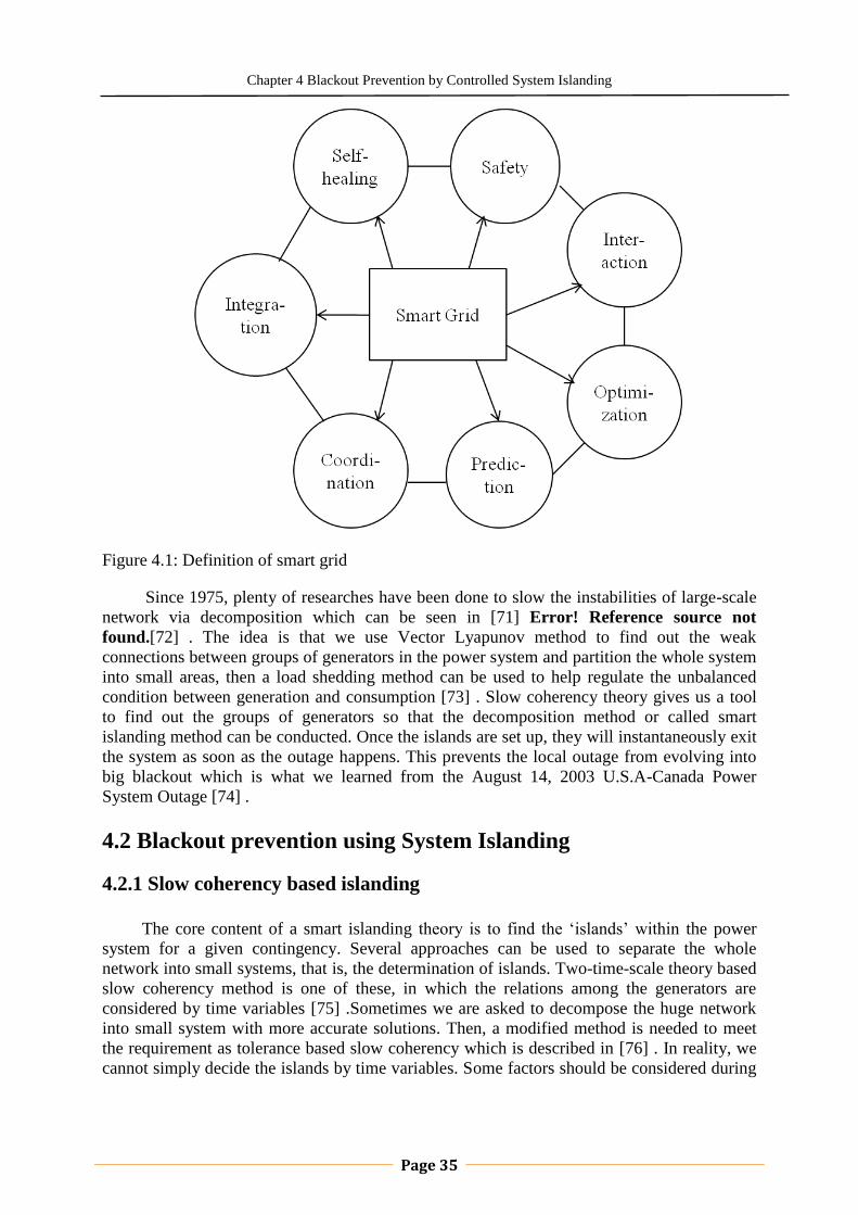
Chapter 4 Blackout Prevention by Controlled System Islanding
Page 35
Figure 4.1: Definition of smart grid
Since 1975, plenty of researches have been done to slow the instabilities of large-scale
network via decomposition which can be seen in [71] Error! Reference source not
found.[72] . The idea is that we use Vector Lyapunov method to find out the weak
connections between groups of generators in the power system and partition the whole system
into small areas, then a load shedding method can be used to help regulate the unbalanced
condition between generation and consumption [73] . Slow coherency theory gives us a tool
to find out the groups of generators so that the decomposition method or called smart
islanding method can be conducted. Once the islands are set up, they will instantaneously exit
the system as soon as the outage happens. This prevents the local outage from evolving into
big blackout which is what we learned from the August 14, 2003 U.S.A-Canada Power
System Outage [74] .
4.2 Blackout prevention using System Islanding
4.2.1 Slow coherency based islanding
The core content of a smart islanding theory is to find the „islands‟ within the power
system for a given contingency. Several approaches can be used to separate the whole
network into small systems, that is, the determination of islands. Two-time-scale theory based
slow coherency method is one of these, in which the relations among the generators are
considered by time variables [75] .Sometimes we are asked to decompose the huge network
into small system with more accurate solutions. Then, a modified method is needed to meet
the requirement as tolerance based slow coherency which is described in [76] . In reality, we
cannot simply decide the islands by time variables. Some factors should be considered during

Chapter 4 Blackout Prevention by Controlled System Islanding
Page 36
the formation of the islands, such as location of a disturbance as well as the physical
constrains [77] . Within these methods, two assumptions are made:
1. The coherent groups of generators are nearly independent of the size of the
disturbance.
2. The coherent groups are independent of the level of detail used in modeling the
generating unit [78] .
The first assumption is based on the observation that the coherency behavior of a
generator is not significantly changed as the clearing time of a specific fault is increased.
While the second assumption is to ensure the generator not to change the basic network
characteristics entirely [79] .
Slow coherency theory essentially is based on the singular perturbation or two-time-
scale method [80] which make it possible for partitioning the system into r weakly connected
areas, in which r means the number of slow coherency groups. After finding the weak
connections, we can apply an automatic islanding algorithm which is based on the slow
coherency method to form the islands [81] [82] [83] [84] [85] .
4.2.2 Smart Islanding using minimal cutsets
The methodology of minimal cutset introduced by Stoer-Wagner [86] has been widely
used in solving the contingency analysis problems. The general description can be explained
as: in an undirected connected network, if we remove an edge set then it can be changed into
two connected components, the edge set is so called cutset, the minimal cutset is the minimal
summation of weighted value.
Classical powers systems are usually consist of buses and transmission lines which
connect each other. The power flow in transmission lines are with different values and
directions. Therefore, we can regard a power system network as a directed graph with
different weights at vertices.
The most critical function of smart islanding is to minimize the real power imbalance
within the islands to benefit the restoration. When an island is created, we can calculate the
imbalance between the real power supply and load demand by computing all the generator
vertices and load vertices [87] however, it requires much more computation and the
calculation process is really time-consuming. The problem can be simplified by taking into
account the branches which are connected to this island without considering the vertex inside
it.
The power flows in the transmission line also contain information of the distribution of
the generators throughout the system. Once the island is formed, the net flow in the tripping
lines indicates exactly how different the real generation and load is within the island (The
losses is not taking into account here). Therefore, the problem has been converted into
searching the minimal cutsets (MCs) to construct the island with the minimal net flow. We
can decompose the islanding problem into two stages:
1. Find Minimal Cutsets;

Chapter 4 Blackout Prevention by Controlled System Islanding
Page 37
2. Obtain Optimal Minimal Cutset by various criteria [88]
4.2.3 Comparisons of several methods used in finding islands
The slow coherency method and minimal cutset method can both be used to form the
islands; the dominant difference is that in slow coherency theory we need to get the
information of the machines while it is not really necessary in the minimal cutset method.
Besides these two methods, some method can be used in solving the problem as well. The
differences among them can be seen as follow:
Table 4.1: Smart islanding methods comparison
Slow coherency smart
partition approach
Slow coherency among the groups of generators does not
vary significantly by the change of initial condition and
disturbance.
The two-time-scale weak connection form inherently
describes the oscillation feature of large-scale power
systems: the fast oscillation within a group of machines
and the slow oscillation between the groups via weak tie
lines.
The slow coherency method also conserves the
characteristics of the coherency-based grouping. It will
not be influenced by the size of the disturbances as well
as detail of the generator model [82] .
Minimum cutset smart
partition approach
o We can decompose the islanding problem into two
phases: Find Minimal Cutsets and Obtain Optimal
Minimal Cutset by various criteria.
o Any additional criteria can be used to formulate the
optimization procedure under different conditions in the
second stage.
o The approach is fully compatible with other techniques.
o User-specified requirements can also be included during
islanding [88] .
Vector Lyapunov method
o Simple numerical algorithm
o Widely used in variety applications ,such as economic
modeling, electric power systems, queueing networks and
computer system
o Suitable for stability analysis[89]

Chapter 4 Blackout Prevention by Controlled System Islanding
Page 38
ordered binary
decision diagrams (OBDDs)
o A directed acyclic graph (DAG) representation of a
Boolean expression.
o It has many advantages to system splitting (SS )
problems or Balanced partition problem (BP) problem
[90]
Hierarch islanding
o Maintaining stable islanding and utilizing the DG
contribution to system availability under conditions of
major systemdisturbance.
o Integrated splitting, real-time load shedding and
resynchronization
o Including Mini Island and Substation Island[91]
4.3 Case study
4.3.1 System description
The model was originally developed with the Powerworld simulator software.In order
to find the „island‟to partition, a C++ minimal cutset algorithm program is compiled and
conducted on the platform of Dev cpp to find the solutions.
4.3.2 Modelling of transmission lines and power flow in Powerworld
In order to find the „island‟, we need first get the total power flow of the test system and
set up a datebase according to the obtained values. In Powerworld, we use a lumped π-
equivalent model to represent the transmission lines, which can be seen in the Fig 4.2 [92]
Figure 4.2: Lumped π-equivalent model of a transmission line and power flowing through it

Chapter 4 Blackout Prevention by Controlled System Islanding
Page 39
The base model used in this work is specified in section 3.4.1 as follows:
a. Power flow equations
Where
: the net active power injected at bus i
: the net reactive power injected at bus i,
: the real part of the element in the line admittance between bus i and j,
the imaginary part of the element in the line admittance between bus i and j,
b. Line flow equations
The active and reactive power flow from bus.i to bus.j can be written as :
While we can get the active and reactive power flow from bus j to bus i in the same
way:
What‟s more, the active and reactive power losses can be computed by using the
following equations:
c. Constraints

Chapter 4 Blackout Prevention by Controlled System Islanding
Page 40
Generation reactive power limits:
Voltage limits:
In Powerworld simulator, we did the simulation by keeping the lower voltage limit to
0.9 p.u and upper voltage limit to 1.1 p.u. The upper limit selection is to avoid insulation
failures while the lower limit is selected by considering the safe margins, however, the lower
limit selection is not as precise as the higher one [93] . The power flow data from Powerworld
can be found in Appendix A.
4.3.3 Enumeration method implemented by Dev cpp
During the simulation process, there are totally 4 main phases in order to find the island
which can be listed as,
1. Implement the Powerworld software and get the power flow data from it.
2. Set up a database for the C++ by using the power flow data.
3. Code compilation
4. Results collection and selection
There are plenty of approaches can be used to find the islands. In this work, we fulfill
the task based on minimal cutset theory.
4.3.3.1 Algorithm and Problem description
The island is formed when the contingency happens. From the analysis in section 3.3.2,
we can see line 4042 to 4043 and 4042 to 4044 undertook the highest risk of overloading.
Hence,we implement the smart islanding according to this fact. By increasing the load on bus
4042 step by step, we can know that the maximum load point, namely collapse point is
1559MW. If more power is injected at this bus, a blackout will be incurred which can be seen
in Figure 4.4. In order to demonstrate the theory of smart islanding, we take the power flow
data which is obtained inmmediately before the blackout. The power flow data is shown in
Appendix B and the condition just before the blackout can be seen in Figure 4.3:
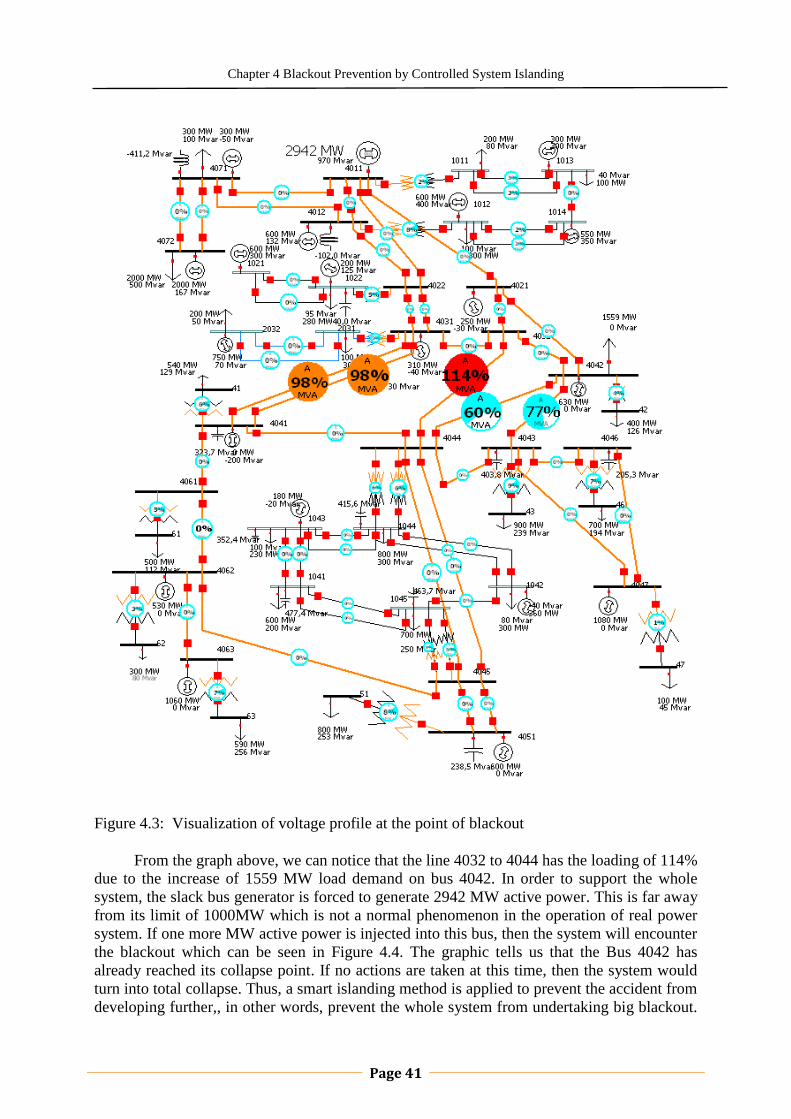
Chapter 4 Blackout Prevention by Controlled System Islanding
Page 41
Figure 4.3: Visualization of voltage profile at the point of blackout
From the graph above, we can notice that the line 4032 to 4044 has the loading of 114%
due to the increase of 1559 MW load demand on bus 4042. In order to support the whole
system, the slack bus generator is forced to generate 2942 MW active power. This is far away
from its limit of 1000MW which is not a normal phenomenon in the operation of real power
system. If one more MW active power is injected into this bus, then the system will encounter
the blackout which can be seen in Figure 4.4. The graphic tells us that the Bus 4042 has
already reached its collapse point. If no actions are taken at this time, then the system would
turn into total collapse. Thus, a smart islanding method is applied to prevent the accident from
developing further,, in other words, prevent the whole system from undertaking big blackout.
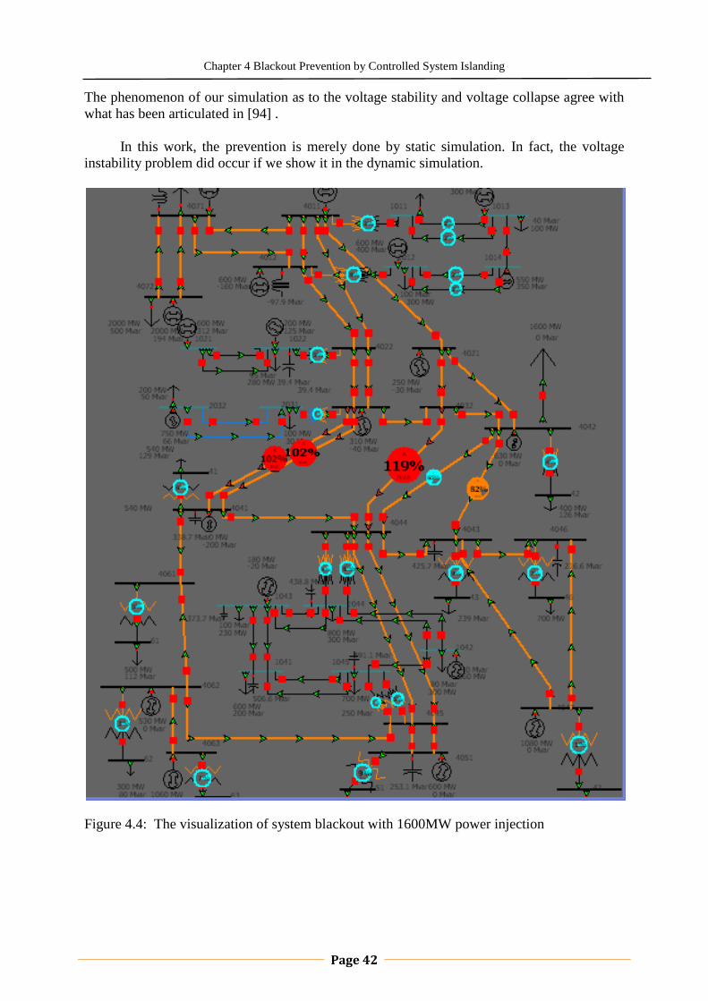
Chapter 4 Blackout Prevention by Controlled System Islanding
Page 42
The phenomenon of our simulation as to the voltage stability and voltage collapse agree with
what has been articulated in [94] .
In this work, the prevention is merely done by static simulation. In fact, the voltage
instability problem did occur if we show it in the dynamic simulation.
Figure 4.4: The visualization of system blackout with 1600MW power injection

Chapter 4 Blackout Prevention by Controlled System Islanding
Page 43
The smart islanding can be implemented by two steps,
The formation of the islands: Find the areas which has the least power interchange
with the others. Hence, it will not affect the other parts a lot when we disconnect this
area.
Disconnet the lines that link the islands: Since the power flow on this lines has no
serious impacts on the other lines, we can disconnect them to protect parts of the
system to work normally.
4.3.3.2 Formation of the islands
It has been presented in section 3.2.1 that the system contains 41 buses. If we assume
that each bus represents a node, then the smart islanding problem can be transferred into a
mathematic model. There are totally 42 nodes connecting each other in one graoh. Each side
has its weight and direction. The objective is to find connected subgraph which meets the
condition that interchange flow among different cutsets is minimum.
As can be seen in Figure 3.3, there are totally 32 buses, namely, 32 nodes within the
system. In fact, the system consists of 41 buses, 9 extra buses are not included in the system,
which are bus 41, 42, 43, 46, 47, 51, 61, 62 and 63. Since they have no relations with the
other buses exvept the buses next to them. We can simplify the model to a 32-node graph
instead of 41 which will reduce the computation time by a great extent.
Based on the theory introduced in section 4.2.2, we employ the minimal cutset
algorithm to find the islands and the algorithm flowchart can be seen in Figure 4.5.
The formulate of the islands was fulfilled by a C++ minimal cutset algorithm program
which is run on the platform of Dev cpp. The program is one citical part of implement the
idea of smart islanding. Therefore, we give a name to this program as „controlled partition
program‟.The input file is shown in Appendix B, Table B.6. The visulization of the original
senario in the normal operating state is shwon in Figure 4.6.
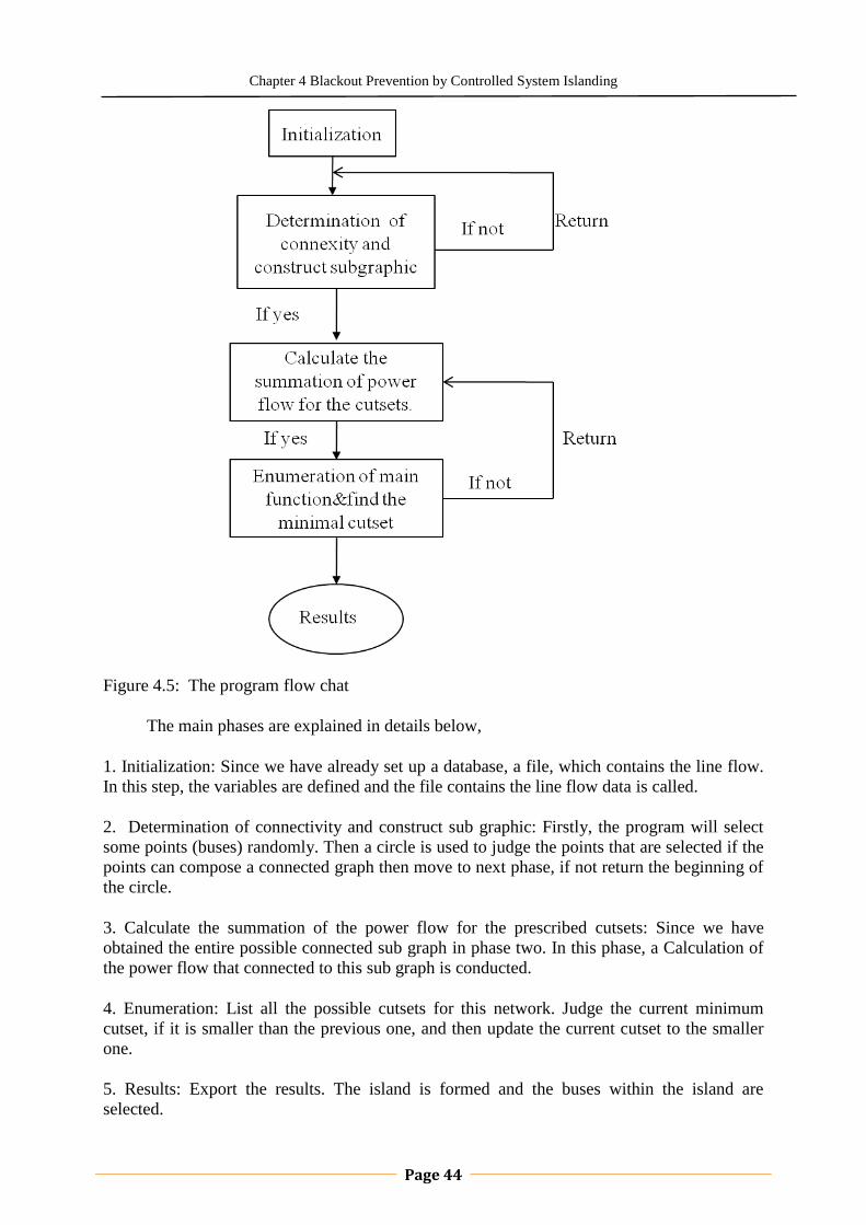
Chapter 4 Blackout Prevention by Controlled System Islanding
Page 44
Figure 4.5: The program flow chat
The main phases are explained in details below,
1. Initialization: Since we have already set up a database, a file, which contains the line flow.
In this step, the variables are defined and the file contains the line flow data is called.
2. Determination of connectivity and construct sub graphic: Firstly, the program will select
some points (buses) randomly. Then a circle is used to judge the points that are selected if the
points can compose a connected graph then move to next phase, if not return the beginning of
the circle.
3. Calculate the summation of the power flow for the prescribed cutsets: Since we have
obtained the entire possible connected sub graph in phase two. In this phase, a Calculation of
the power flow that connected to this sub graph is conducted.
4. Enumeration: List all the possible cutsets for this network. Judge the current minimum
cutset, if it is smaller than the previous one, and then update the current cutset to the smaller
one.
5. Results: Export the results. The island is formed and the buses within the island are
selected.
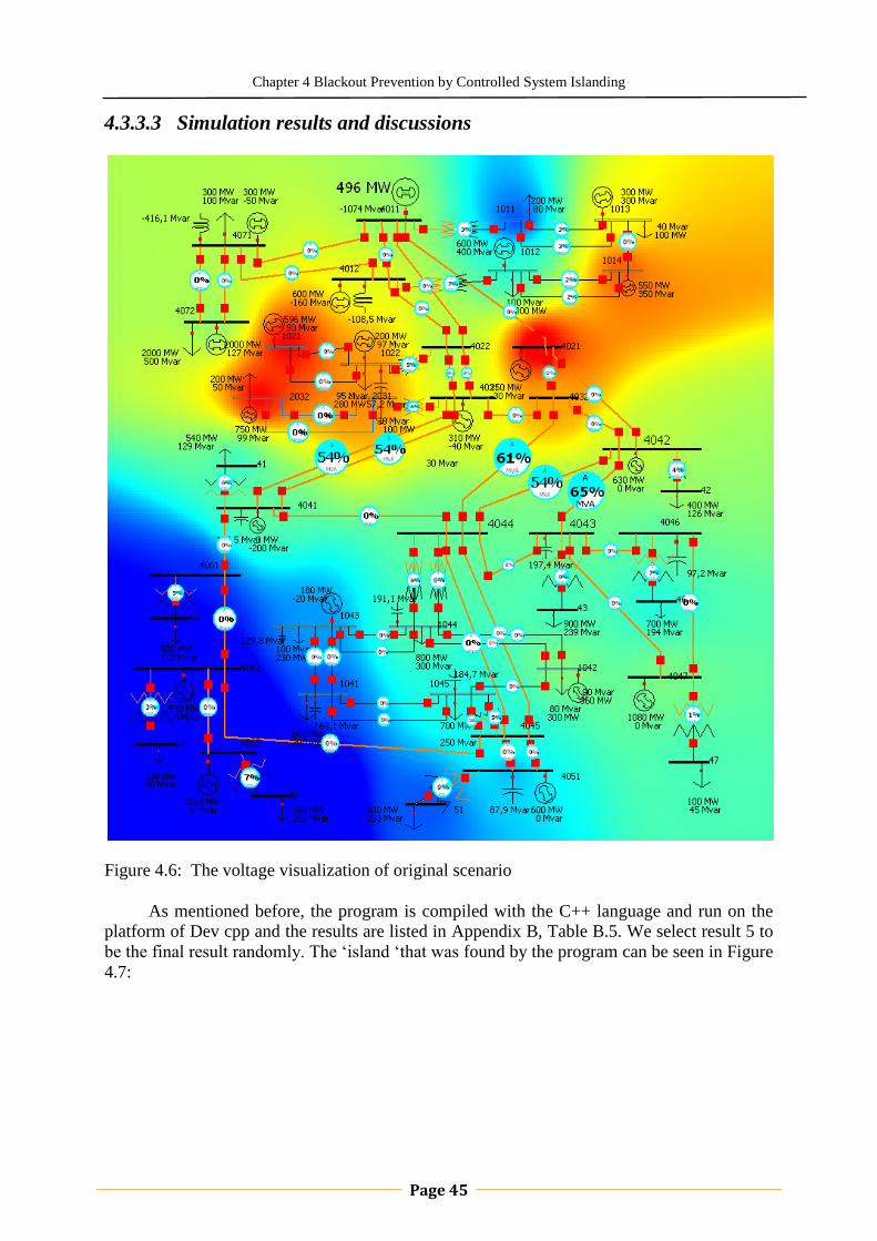
Chapter 4 Blackout Prevention by Controlled System Islanding
Page 45
4.3.3.3 Simulation results and discussions
Figure 4.6: The voltage visualization of original scenario
As mentioned before, the program is compiled with the C++ language and run on the
platform of Dev cpp and the results are listed in Appendix B, Table B.5. We select result 5 to
be the final result randomly. The „island „that was found by the program can be seen in Figure
4.7:
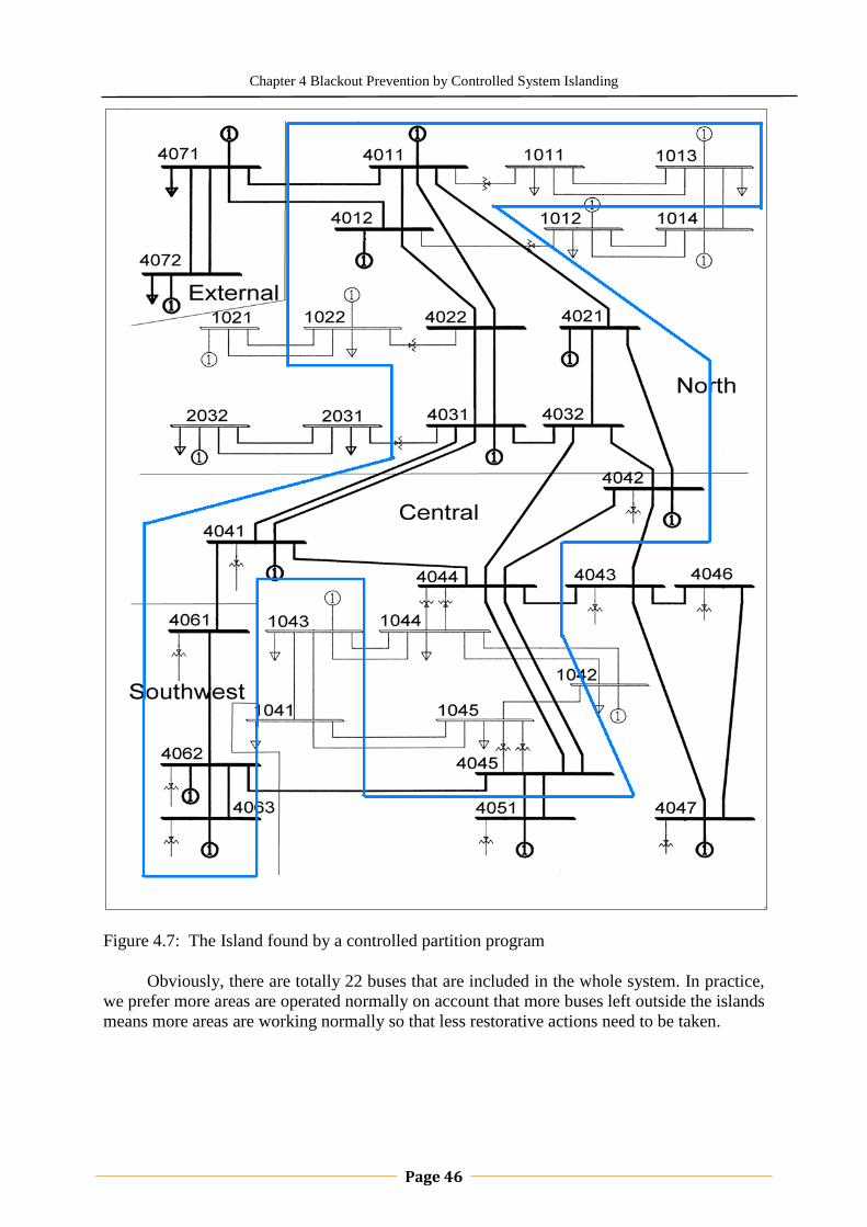
Chapter 4 Blackout Prevention by Controlled System Islanding
Page 46
Figure 4.7: The Island found by a controlled partition program
Obviously, there are totally 22 buses that are included in the whole system. In practice,
we prefer more areas are operated normally on account that more buses left outside the islands
means more areas are working normally so that less restorative actions need to be taken.

Chapter 4 Blackout Prevention by Controlled System Islanding
Page 47
Figure 4.8: Minimal net flow V.S Island‟s sizes
In order to get an approximately relations between the number of buses included within
the islands and the net active power flow. We change the program to find the islands with
different sizes which is compared in Figure 4.8. The results of different islands can be seen in
Appendix B.
Based on the simulation‟s results, it is not hard to say that more buses included in the
island, less power interchange with the other parts it will be. In other words, more buses in the
cutset can keep the imbalance of load and generation to a relative lower value. The objective
function of the program is to minimize the net flow while our task is to keep as many as rest
power system work normally after the islands are formed. The computer gives us a cutset
which meets the requirement that the net power flow is minimal, however, as we knew that
there is a trade-off between the number of buses included and the minimum net power flow.
One task left for us in practical is to find the optimal solution to satisfy different scenarios
under different situations.
4.3.4 Modified islands’ model
In order to prevent the total collapse, a modified model is constructed as in Figure 4.9.
0
0,1
0,2
0,3
0,4
0,5
0,6
0,7
8 buses 12 buses 15 buses
Net Active Power Flow(MW)
MW
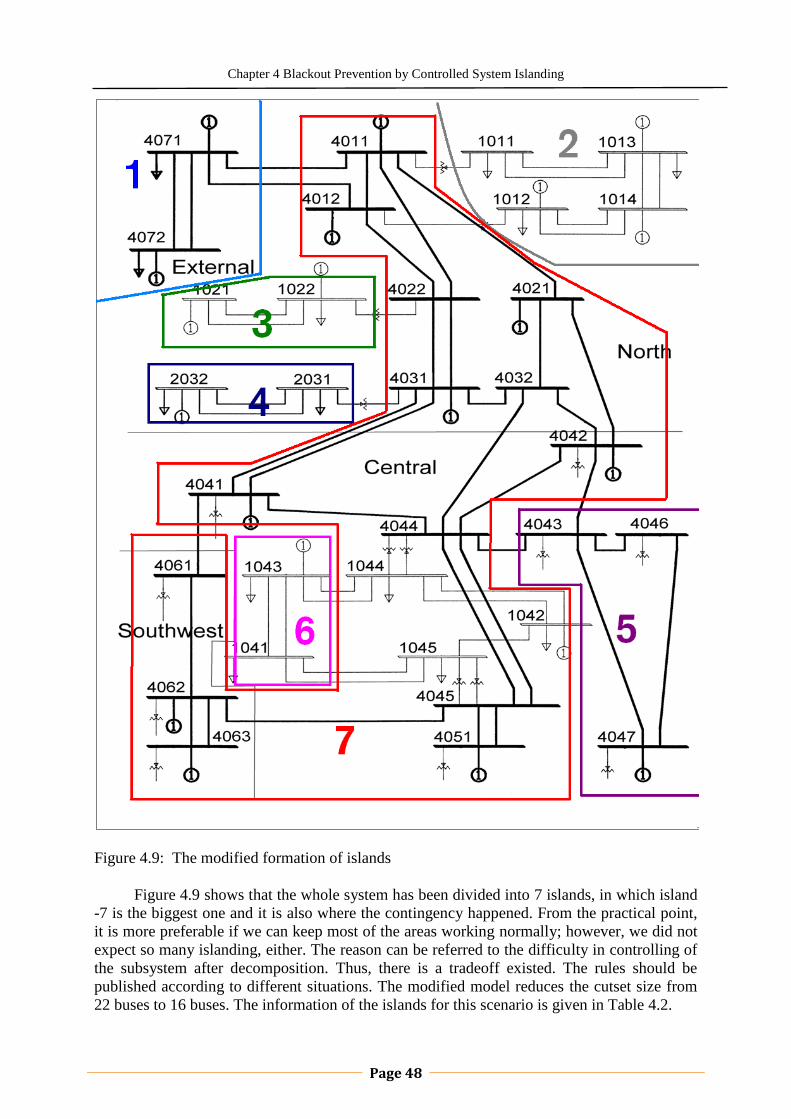
Chapter 4 Blackout Prevention by Controlled System Islanding
Page 48
Figure 4.9: The modified formation of islands
Figure 4.9 shows that the whole system has been divided into 7 islands, in which island
-7 is the biggest one and it is also where the contingency happened. From the practical point,
it is more preferable if we can keep most of the areas working normally; however, we did not
expect so many islanding, either. The reason can be referred to the difficulty in controlling of
the subsystem after decomposition. Thus, there is a tradeoff existed. The rules should be
published according to different situations. The modified model reduces the cutset size from
22 buses to 16 buses. The information of the islands for this scenario is given in Table 4.2.
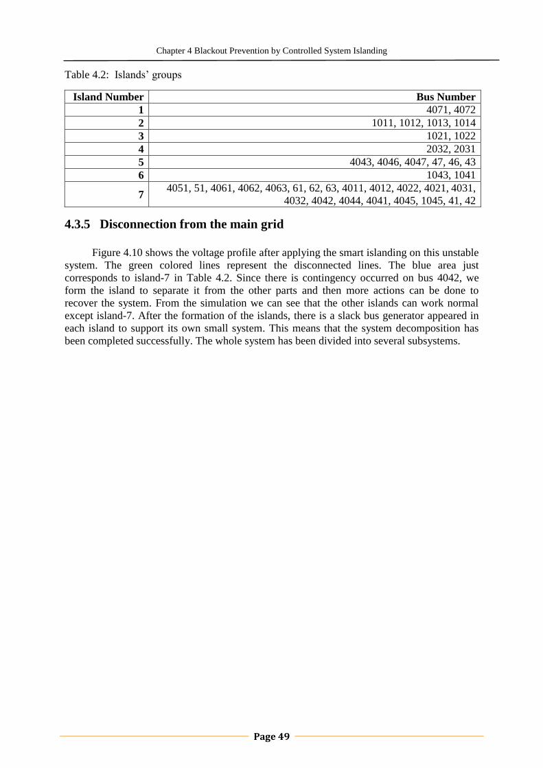
Chapter 4 Blackout Prevention by Controlled System Islanding
Page 49
Table 4.2: Islands‟ groups
Island Number Bus Number
1 4071, 4072
2 1011, 1012, 1013, 1014
3 1021, 1022
4 2032, 2031
5 4043, 4046, 4047, 47, 46, 43
6 1043, 1041
7 4051, 51, 4061, 4062, 4063, 61, 62, 63, 4011, 4012, 4022, 4021, 4031,
4032, 4042, 4044, 4041, 4045, 1045, 41, 42
4.3.5 Disconnection from the main grid
Figure 4.10 shows the voltage profile after applying the smart islanding on this unstable
system. The green colored lines represent the disconnected lines. The blue area just
corresponds to island-7 in Table 4.2. Since there is contingency occurred on bus 4042, we
form the island to separate it from the other parts and then more actions can be done to
recover the system. From the simulation we can see that the other islands can work normal
except island-7. After the formation of the islands, there is a slack bus generator appeared in
each island to support its own small system. This means that the system decomposition has
been completed successfully. The whole system has been divided into several subsystems.
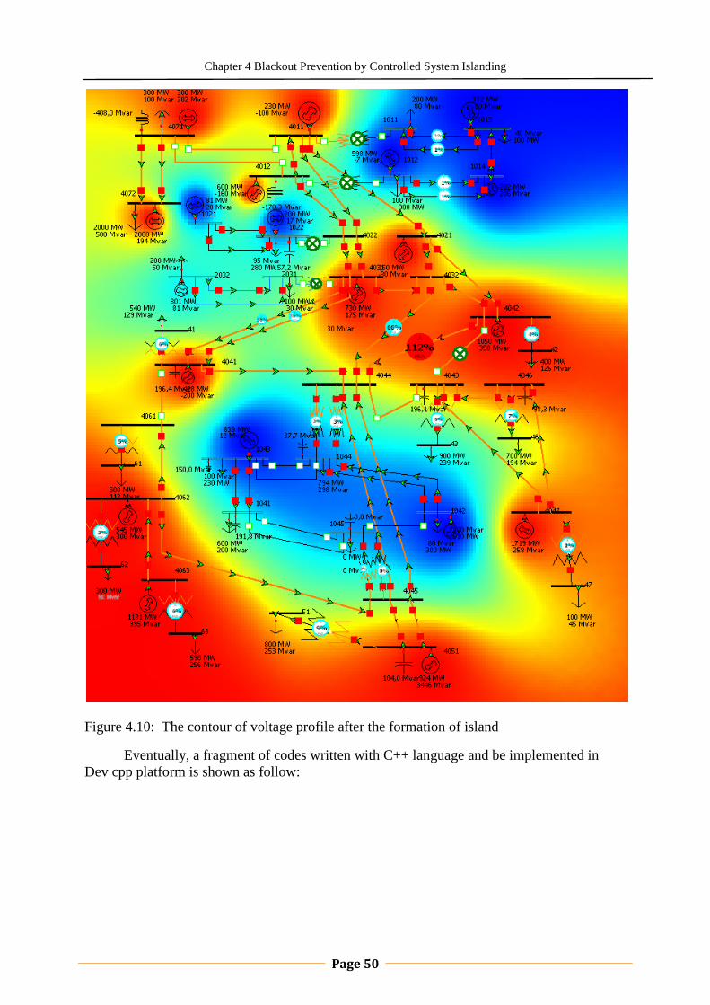
Chapter 4 Blackout Prevention by Controlled System Islanding
Page 50
Figure 4.10: The contour of voltage profile after the formation of island
Eventually, a fragment of codes written with C++ language and be implemented in
Dev cpp platform is shown as follow:

Chapter 4 Blackout Prevention by Controlled System Islanding
Page 51
Controlled Partition Program
void initial() //Initialzation,definition of variables
{
char buf[MAXNUM_BUF];
char namebuf1[MAXNUM_BUF] , namebuf2[MAXNUM_BUF];
string name1 , name2;
int pos1 , pos2;
double tmp;
string rstName;
name2pos.clear();
for( int i = 0; i < MAXNUM_POINT; ++i )//
pos2name[i] = "";
memset( graph , 0 , sizeof( graph ) );
memset( edge , 0 , sizeof( edge ) );
nPoint = 0;
int64 cnt;
priority queue<RESULT>qu;
const int quSize = 20;
fIn = fopen( "line_flow_data_32.txt" , "r" );//Input the line flow
data which has already been set up previously
string fileName;
time_t currentTime = time(0);
string timeStr;
timeStr = (string)(ctime(¤tTime));
timeStr = timeStr.substr(0,timeStr.length() - 1 );
for(int i = 0; i < timeStr.length(); ++i)
if( timeStr[i] == ':' || timeStr[i] == ' ' )
timeStr[i] = '_';
fileName = "result_" + timeStr + ".txt
fOut = fopen( fileName.c_str() , "w" );
while( fgets( buf , MAXNUM_BUF , fIn ) != NULL ){
sscanf( buf , "%s%s%*d%lf" , namebuf1 , namebuf2 , &tmp );
name1 = (string)namebuf1;
name2 = (string)namebuf2;
if( name2pos.find(name1) == name2pos.end() ){
name2pos[name1] = nPoint;
pos1 = nPoint;
nPoint++;
}else{
pos1 = name2pos[name1];
}

Chapter 4 Blackout Prevention by Controlled System Islanding
Page 52
pos2name[pos1] = name1;
if( name2pos.find(name2) == name2pos.end() ){
name2pos[name2] = nPoint;
pos2 = nPoint;
nPoint++;
}else{
pos2 = name2pos[name2];
}
pos2name[pos2] = name2;
graph[pos1][pos2] = graph[pos2][pos1] = 1;
edge[pos1][pos2] = (int)( tmp * 10000 );
}
}
void dfs( int u , int64 statei )// searching the points to see if
they are connected or not
{
int i;
for( i = 0; i < nPoint; ++i )
if( ( subClr & (1LL<<i) ) == 0 &&
( statei & (1LL<<i) ) != 0 &&
graph[u][i] != 0 ){
subClr |= 1LL<<i;
dfs( i , statei );
}
}
inline bool isConnect( int64 statei )//Judgment of connectivity
{
subClr = 0;
int i;
for( i = 0; i < nPoint; ++i )
if( ( subClr & (1LL<<i) ) == 0 &&
( statei & (1LL<<i) ) != 0 ){
subClr |= 1LL<<i;
dfs( i , statei );
break;
}
return statei == subClr;
}

Chapter 4 Blackout Prevention by Controlled System Islanding
Page 53
void process( int tmpNPoint )//calculation the weight of the summation
of nodes
{
nPoint = tmpNPoint
;
int i , j;
memset( value , 0 , sizeof( value ) );
for( i = 0; i < nPoint; ++i )
for( j = 0; j < nPoint; ++j ){
value[i] -= edge[i][j];
value[j] += edge[i][j];
}
}
inline bool cnt1valid( int64 statei )//calculation the number of nodes
{
int cnt = 0;
while( statei ){
cnt++;
statei = statei & ( statei - 1 );
}
return cnt >= 6 && cnt <= 12;
}
int64 cnt;
void findRst()//Enumeration of the main function,find the minimal
cutset
{
int64 statei;
int rst , tmpRst;
int64 rstState;
priority queue<RESULT>qu;
const int quSize = 20;
rst = 0x7fffffff;
cnt = 0;
for( statei = 1; statei < ( ( 1LL<<nPoint) - 1 );++statei ){
if( statei % 10000000LL == 0 ){
printf( "mission completed : %.2lf%%\n" , ((double)statei /
(double)((1LL<<nPoint)-1) ) * 100.0 );
}
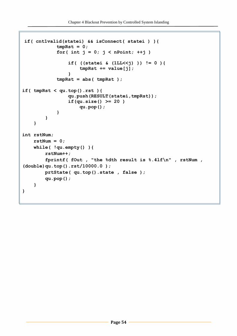
Chapter 4 Blackout Prevention by Controlled System Islanding
Page 54
if( cnt1valid(statei) && isConnect( statei ) ){ tmpRst = 0;
for( int j = 0; j < nPoint; ++j )
if( ((statei & (1LL<<j) )) != 0 ){
tmpRst += value[j];
}
tmpRst = abs( tmpRst );
if( tmpRst < qu.top().rst ){
qu.push(RESULT(statei,tmpRst));
if(qu.size() >= 20 )
qu.pop();
}
}
}
int rstNum;
rstNum = 0;
while( !qu.empty() ){
rstNum++;
fprintf( fOut , "the %dth result is %.4lf\n" , rstNum ,
(double)qu.top().rst/10000.0 );
prtState( qu.top().state , false );
qu.pop();
}
}
Page 55
Chapter 5
Conclusions and Future Work
5.1 Conclusions
Since the energy crisis of 1973, people realize that the depletion of non-renewable
resource will have significant impact on human beings‟ life. Hence, more and more concerns
are given on the utilization of new sustainable resources to replace the existing ones. As a
clean renewable resource, wind power, which has less impact on the environment than the
other resources that can be used in electricity generation industry, moreover, the ever-
increasing load demand asked for a new form of generation as well. Hence, people shows
more interests in the application of wind power generation and governments has begun to
increase the proportion of wind generation in the total national generation. However, in order
to create more economic benefits to the society, we need to think out the blueprint of a wind
power project. One overriding issue to be deliberated is the selection of good locations and
the amounts of new injections on each position.
At the beginning, this thesis introduced the WTLR/ETLR sensitivity methodology
which gives us good indicators to select the best locations to inject. The results present that
the right selection can not only balance the load increase by local generation but also mitigate
the contingency overload. The overall loading of the contingency lines are proved to be
mitigated by the new injections, however, in some scenario, the loading of certain line is
increased though the overall loading is decreased. This is due to the fact that the TLR of each
contingency line is not always with the same sign. The positive sign will increase the power
flow on that line when inject at a specific bus and vice verse. The reduction of the loading on
the contingency lines has two meanings: on one hand, it increase the power system security
by making the line transmit power far away from its transmission limit and maintain the
system to operate more securely. On the other hand, the reduction of the loading leaves a safe
margin for the transmission lines which is the enhancement of the system adequacy. This
action increases the power system reliability at some extent. The optimal places are selected
according to the value of WTLR/ETLR sensitivity, all places with minus value can be
selected as the injection point, however, the decision should be made based on the local
climax and local generation price as well. Several scenarios were made up to demonstrate our
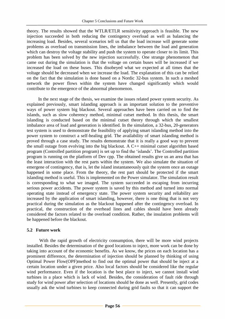
Chapter 5 Conclusions and Future Work
Page 56
theory. The results showed that the WTLR/ETLR sensitivity approach is feasible. The new
injection succeeded in both reducing the contingency overload as well as balancing the
increasing load. Besides, several scenarios tell us that the load increase will generate some
problems as overload on transmission lines, the imbalance between the load and generation
which can destroy the voltage stability and push the system to operate closer to its limit. This
problem has been solved by the new injection successfully. One strange phenomenon that
came out during the simulation is that the voltage on certain buses will be increased if we
increased the load on these buses. This disobeyed what we expected at all times that the
voltage should be decreased when we increase the load. The explanation of this can be relied
on the fact that the simulation is done based on a Nordic 32-bus system. In such a meshed
network the power flows within the system have changed significantly which would
contribute to the emergence of the abnormal phenomenon.
In the next stage of the thesis, we examine the issues related power system security. As
explained previously, smart islanding approach is an important solution to the preventive
ways of power system big blackout. Several approaches have been carried on to find the
islands, such as slow coherency method, minimal cutset method. In this thesis, the smart
islanding is conducted based on the minimal cutset theory through which the smallest
imbalance area of load and generation is identified. In the simulation, a 32-bus, 20-generators
test system is used to demonstrate the feasibility of applying smart islanding method into the
power system to construct a self-healing grid. The availability of smart islanding method is
proved through a case study. The results demonstrate that it is really a good way to prevent
the small outage from evolving into the big blackout. A C++ minimal cutset algorithm based
program (Controlled partition program) is set up to find the „islands‟. The Controlled partition
program is running on the platform of Dev cpp. The obtained results give us an area that has
the least interaction with the rest parts within the system. We also simulate the situation of
emergene of contingency, that is, let the island instantaneously quit the system once an outage
happened in some place. From the theory, the rest part should be protected if the smart
islanding method is useful. This is implemented on the Power simulator. The simulation result
is corresponding to what we imaged. The system succeeded in escaping from incurring
serious power accidents. The power system is saved by this method and turned into normal
operating state instead of emergency state. The power system security and reliability are
increased by the application of smart islanding, however, there is one thing that is not very
practical during the simulation as the blackout happened after the contingency overload. In
practical, the construction of the overhead lines and cables should have been already
considered the factors related to the overload condition. Rather, the insulation problems will
be happened before the blackout.
5.2 Future work
With the rapid growth of electricity consumption, there will be more wind projects
installed. Besides the determination of the good locations to inject, more work can be done by
taking into account of the economic benefits. As we know, the prices on each location has a
prominent difference, the determination of injection should be planned by thinking of using
Optimal Power Flow(OPF)method to find out the optimal power that should be inject at a
certain location under a given price. Also local factors should be considered like the regular
wind performance. Even if the location is the best place to inject, we cannot install wind
turbines in a place which is lack of wind. Besides, the consideration of fault ride through
study for wind power after selection of locations should be done as well. Presently, grid codes
usually ask the wind turbines to keep connected during grid faults so that it can support the

Chapter 5 Conclusions and Future Work
Page 57
system till the fault is cleared. The wind turbines must be designed to withstand the voltage
disturbances. More work should be done after the integration of wind energy into the existing
grid in future work.
On the other hand, the smart islanding prevents the emerge of big blackout, however,
more attentions should be paid after the formation of the islands. In load-rich islands, a load
shedding scheme is usually used while the generation shedding scheme is applied in a
generation-rich island. More work can be done in dynamic simulation of the system in
combination of islanding algorithm. As showed in the previous work, certain measures can be
used to protect the system from a total collapse, as modification of protection setting, smart
islanding, circuit-breaker blocking, tap-changers transformers blocking and loading shedding.
The loading shedding and circuit-breaker blocking measures have already been done in [94]
In future, dynamic simulation of voltage and frequency control during the blackout combing
with smart islanding method to prevent total collapse can be done under the help of Advanced
real-time Interactive Simulator for Training and Operation (ARISTO) system.
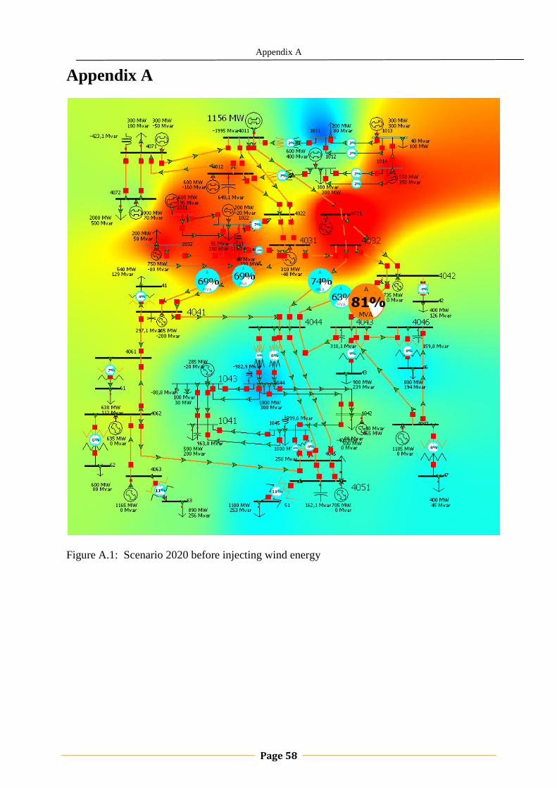
Appendix A
Page 58
Appendix A
Figure A.1: Scenario 2020 before injecting wind energy

Appendix A
Page 59
Figure A.2: Scenario 2020 after injecting wind energy
Table A.1: Voltage profile of test system for 2010
Voltage profile
Bus Voltage
(p.u)
Bus Voltage
(p.u)
Bus Voltage
(p.u)
Bus Voltage
(p.u)
41 1.03 1012 0.97 1041 0.90 2031 1.10
42 1.03 1013 1.05 1042 1.00 2032 1.10
43 0.99 1014 1.08 1043 0.92 4011 1.01
46 0.98 1021 1.10 1044 0.98 4012 1.04
47 0.99 1022 1.07 1045 0.97 4021 1.13
51 0.97 4022 1.03 4043 1.01 4051 0.98
61 1.02 4031 1.06 4044 1.00 4061 1.04
62 1.02 4032 1.09 4045 0.99 4062 1.04

Appendix A
Page 60
63 1.00 4041 1.04 4046 1.00 4063 1.02
1011 0.92 4042 1.05 4047 1.01 4071 1.02
4072 1.01
Table A.2: Voltage profile of test system for 2015
Voltage profile
Bus Voltage
(p.u)
Bus Voltage
(p.u)
Bus Voltage
(p.u)
Bus Voltage
(p.u)
41 1.02 1013 1.05 2032 1.10 4044 0.98
42 1.01 1014 1.08 4011 1.01 4045 0.97
43 0.96 1021 1.10 4012 1.04 4046 0.97
46 0.94 1022 1.10 4021 1.12 4047 0.98
47 0.95 1041 0.93 4022 1.03 4051 0.95
51 0.94 1042 1.00 4031 1.06 4061 1.02
61 1.01 1043 0.90 4032 1.08 4062 1.03
62 1.01 1044 0.95 4041 1.03 4063 1.01
63 1.00 1045 0.95 4042 1.02 4071 1.02
1011 0.92 2031 1.09 4043 0.98 4072 1.01
1012 0.97
Table A.3: Voltage profile of test system for 2020
Voltage profile
Bus Voltage
(p.u) Bus
Voltage
(p.u) Bus
Voltage
(p.u) Bus
Voltage
(p.u)
41 0.99 1013 1.04 2032 1.10 4044 0.98
42 0.99 1014 1.07 4011 1.01 4045 0.97
43 0.94 1021 1.10 4012 1.01 4046 0.93
46 0.91 1022 1.07 4021 1.09 4047 0.94
47 0.91 1041 1.08 4022 1.01 4051 0.94
51 0.93 1042 1.00 4031 1.03 4061 1.00
61 0.98 1043 1.03 4032 1.06 4062 1.01
62 0.99 1044 0.97 4041 1.00 4063 1.01
63 1.00 1045 0.95 4042 1.01 4071 1.01
1011 0.92 2031 1.07 4043 0.96 4072 1.01
1012 0.95
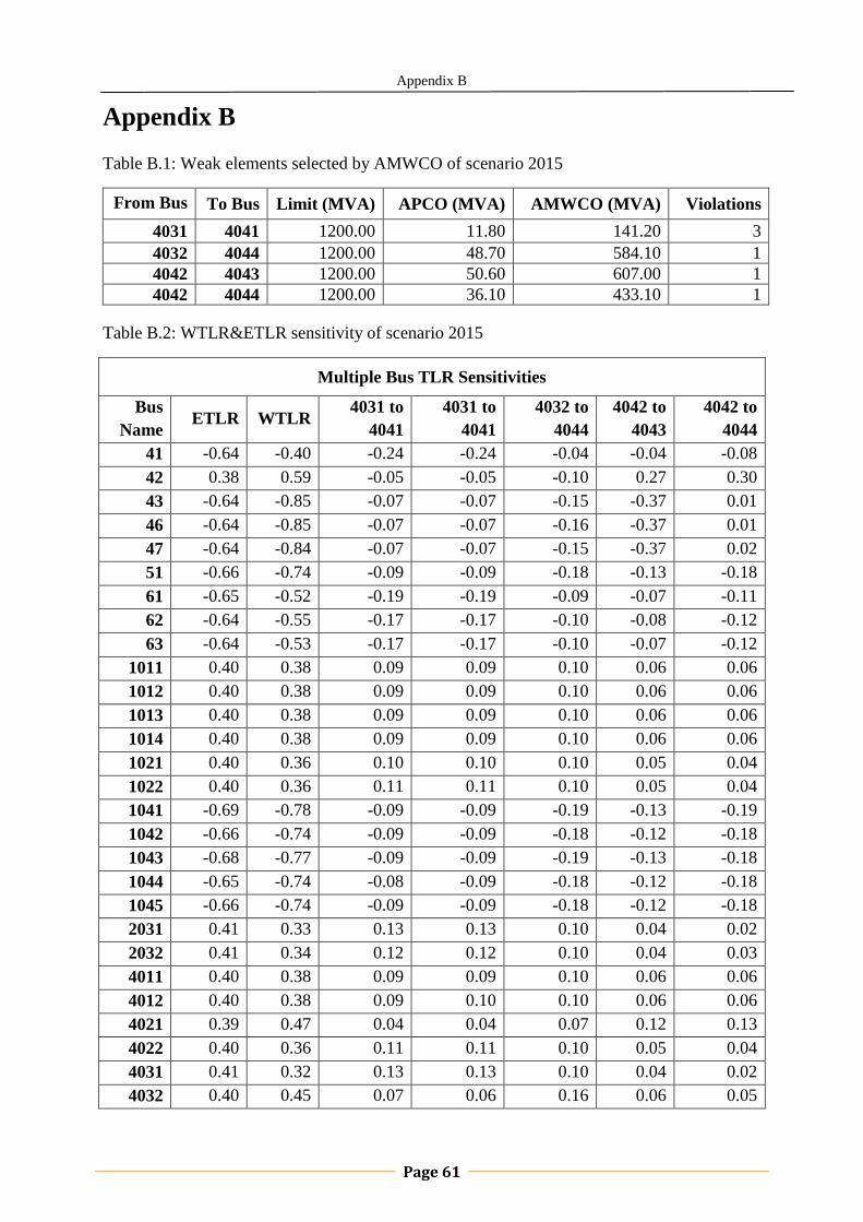
Appendix B
Page 61
Appendix B
Table B.1: Weak elements selected by AMWCO of scenario 2015
From Bus To Bus Limit (MVA) APCO (MVA) AMWCO (MVA) Violations
4031 4041 1200.00 11.80 141.20 3
4032 4044 1200.00 48.70 584.10 1
4042 4043 1200.00 50.60 607.00 1
4042 4044 1200.00 36.10 433.10 1
Table B.2: WTLR&ETLR sensitivity of scenario 2015
Multiple Bus TLR Sensitivities
Bus
Name ETLR WTLR
4031 to
4041
4031 to
4041
4032 to
4044
4042 to
4043
4042 to
4044
41 -0.64 -0.40 -0.24 -0.24 -0.04 -0.04 -0.08
42 0.38 0.59 -0.05 -0.05 -0.10 0.27 0.30
43 -0.64 -0.85 -0.07 -0.07 -0.15 -0.37 0.01
46 -0.64 -0.85 -0.07 -0.07 -0.16 -0.37 0.01
47 -0.64 -0.84 -0.07 -0.07 -0.15 -0.37 0.02
51 -0.66 -0.74 -0.09 -0.09 -0.18 -0.13 -0.18
61 -0.65 -0.52 -0.19 -0.19 -0.09 -0.07 -0.11
62 -0.64 -0.55 -0.17 -0.17 -0.10 -0.08 -0.12
63 -0.64 -0.53 -0.17 -0.17 -0.10 -0.07 -0.12
1011 0.40 0.38 0.09 0.09 0.10 0.06 0.06
1012 0.40 0.38 0.09 0.09 0.10 0.06 0.06
1013 0.40 0.38 0.09 0.09 0.10 0.06 0.06
1014 0.40 0.38 0.09 0.09 0.10 0.06 0.06
1021 0.40 0.36 0.10 0.10 0.10 0.05 0.04
1022 0.40 0.36 0.11 0.11 0.10 0.05 0.04
1041 -0.69 -0.78 -0.09 -0.09 -0.19 -0.13 -0.19
1042 -0.66 -0.74 -0.09 -0.09 -0.18 -0.12 -0.18
1043 -0.68 -0.77 -0.09 -0.09 -0.19 -0.13 -0.18
1044 -0.65 -0.74 -0.08 -0.09 -0.18 -0.12 -0.18
1045 -0.66 -0.74 -0.09 -0.09 -0.18 -0.12 -0.18
2031 0.41 0.33 0.13 0.13 0.10 0.04 0.02
2032 0.41 0.34 0.12 0.12 0.10 0.04 0.03
4011 0.40 0.38 0.09 0.09 0.10 0.06 0.06
4012 0.40 0.38 0.09 0.10 0.10 0.06 0.06
4021 0.39 0.47 0.04 0.04 0.07 0.12 0.13
4022 0.40 0.36 0.11 0.11 0.10 0.05 0.04
4031 0.41 0.32 0.13 0.13 0.10 0.04 0.02
4032 0.40 0.45 0.07 0.06 0.16 0.06 0.05
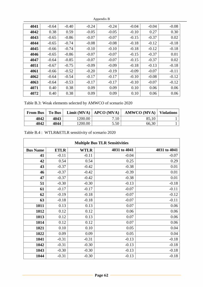
Appendix B
Page 62
4041 -0.64 -0.40 -0.24 -0.24 -0.04 -0.04 -0.08
4042 0.38 0.59 -0.05 -0.05 -0.10 0.27 0.30
4043 -0.65 -0.86 -0.07 -0.07 -0.15 -0.37 0.02
4044 -0.65 -0.74 -0.08 -0.08 -0.18 -0.12 -0.18
4045 -0.66 -0.74 -0.10 -0.10 -0.18 -0.12 -0.18
4046 -0.65 -0.86 -0.07 -0.07 -0.15 -0.37 0.01
4047 -0.64 -0.85 -0.07 -0.07 -0.15 -0.37 0.02
4051 -0.67 -0.75 -0.09 -0.09 -0.18 -0.13 -0.18
4061 -0.66 -0.52 -0.20 -0.19 -0.09 -0.07 -0.11
4062 -0.64 -0.54 -0.17 -0.17 -0.10 -0.08 -0.12
4063 -0.64 -0.53 -0.17 -0.17 -0.10 -0.07 -0.12
4071 0.40 0.38 0.09 0.09 0.10 0.06 0.06
4072 0.40 0.38 0.09 0.09 0.10 0.06 0.06
Table B.3: Weak elements selected by AMWCO of scenario 2020
From Bus To Bus Limit (MVA) APCO (MVA) AMWCO (MVA) Violations
4042 4043 1200.00 7.10 85,10 1
4042 4044 1200.00 5.50 66,30 1
Table B.4 : WTLR&ETLR sensitivity of scenario 2020
Multiple Bus TLR Sensitivities
Bus Name ETLR WTLR 4031 to 4041 4031 to 4041
41 -0.11 -0.11 -0.04 -0.07
42 0.54 0.54 0.25 0.29
43 -0.37 -0.42 -0.38 0.01
46 -0.37 -0.42 -0.39 0.01
47 -0.37 -0.42 -0.38 0.01
51 -0.30 -0.30 -0.13 -0.18
61 -0.17 -0.17 -0.07 -0.11
62 -0.19 -0.18 -0.07 -0.12
63 -0.18 -0.18 -0.07 -0.11
1011 0.13 0.13 0.07 0.06
1012 0.12 0.12 0.06 0.06
1013 0.12 0.13 0.07 0.06
1014 0.12 0.12 0.07 0.06
1021 0.10 0.10 0.05 0.04
1022 0.09 0.09 0.05 0.04
1041 -0.31 -0.31 -0.13 -0.18
1042 -0.31 -0.30 -0.13 -0.18
1043 -0.30 -0.30 -0.13 -0.18
1044 -0.31 -0.30 -0.13 -0.18
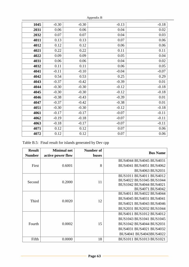
Appendix B
Page 63
1045 -0.30 -0.30 -0.13 -0.18
2031 0.06 0.06 0.04 0.02
2032 0.07 0.07 0.04 0.03
4011 0.13 0.13 0.07 0.06
4012 0.12 0.12 0.06 0.06
4021 0.22 0.22 0.11 0.11
4022 0.09 0.09 0.05 0.04
4031 0.06 0.06 0.04 0.02
4032 0.11 0.11 0.06 0.05
4041 -0.11 -0.10 -0.04 -0.07
4042 0.54 0.53 0.25 0.29
4043 -0.37 -0.42 -0.39 0.01
4044 -0.30 -0.30 -0.12 -0.18
4045 -0.30 -0.30 -0.12 -0.18
4046 -0.38 -0.43 -0.39 0.01
4047 -0.37 -0.42 -0.38 0.01
4051 -0.30 -0.30 -0.12 -0.18
4061 -0.17 -0.17 -0.07 -0.11
4062 -0.19 -0.18 -0.07 -0.11
4063 -0.18 -0.17 -0.07 -0.11
4071 0.12 0.12 0.07 0.06
4072 0.12 0.12 0.07 0.06
Table B.5: Final result for islands generated by Dev cpp
Result
Number
Minimal net
active power flow
Number of
buses Bus Name
First 0.6001 8
BUS4044 BUS4045 BUS4031
BUS4041 BUS4051 BUS4062
BUS4063 BUS2031
Second 0.2000 11
BUS1011 BUS4011 BUS4012
BUS4022 BUS1045 BUS1044
BUS1042 BUS4044 BUS4021
BUS4071 BUS4042
Third 0.0020 12
BUS4011 BUS4022 BUS4044
BUS4045 BUS4031 BUS4041
BUS4021 BUS4043 BUS4046
BUS2031 BUS2032 BUS1044
Fourth 0.0002 15
BUS4011 BUS1012 BUS4012
BUS1043 BUS1041 BUS1045
BUS1042 BUS4044 BUS2031
BUS4031 BUS4021 BUS4032
BUS4041 BUS4043BUS4022
Fifth 0.0000 18 BUS1011 BUS1013 BUS1021
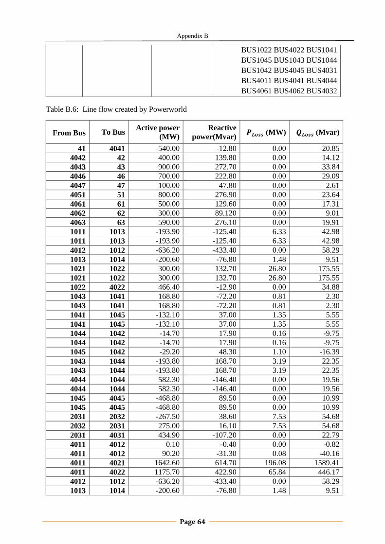
Appendix B
Page 64
BUS1022 BUS4022 BUS1041
BUS1045 BUS1043 BUS1044
BUS1042 BUS4045 BUS4031
BUS4011 BUS4041 BUS4044
BUS4061 BUS4062 BUS4032
Table B.6: Line flow created by Powerworld
From Bus To Bus Active power
(MW)
Reactive
power(Mvar) (MW) (Mvar)
41 4041 -540.00 -12.80 0.00 20.85
4042 42 400.00 139.80 0.00 14.12
4043 43 900.00 272.70 0.00 33.84
4046 46 700.00 222.80 0.00 29.09
4047 47 100.00 47.80 0.00 2.61
4051 51 800.00 276.90 0.00 23.64
4061 61 500.00 129.60 0.00 17.31
4062 62 300.00 89.120 0.00 9.01
4063 63 590.00 276.10 0.00 19.91
1011 1013 -193.90 -125.40 6.33 42.98
1011 1013 -193.90 -125.40 6.33 42.98
4012 1012 -636.20 -433.40 0.00 58.29
1013 1014 -200.60 -76.80 1.48 9.51
1021 1022 300.00 132.70 26.80 175.55
1021 1022 300.00 132.70 26.80 175.55
1022 4022 466.40 -12.90 0.00 34.88
1043 1041 168.80 -72.20 0.81 2.30
1043 1041 168.80 -72.20 0.81 2.30
1041 1045 -132.10 37.00 1.35 5.55
1041 1045 -132.10 37.00 1.35 5.55
1044 1042 -14.70 17.90 0.16 -9.75
1044 1042 -14.70 17.90 0.16 -9.75
1045 1042 -29.20 48.30 1.10 -16.39
1043 1044 -193.80 168.70 3.19 22.35
1043 1044 -193.80 168.70 3.19 22.35
4044 1044 582.30 -146.40 0.00 19.56
4044 1044 582.30 -146.40 0.00 19.56
1045 4045 -468.80 89.50 0.00 10.99
1045 4045 -468.80 89.50 0.00 10.99
2031 2032 -267.50 38.60 7.53 54.68
2032 2031 275.00 16.10 7.53 54.68
2031 4031 434.90 -107.20 0.00 22.79
4011 4012 0.10 -0.40 0.00 -0.82
4011 4012 90.20 -31.30 0.08 -40.16
4011 4021 1642.60 614.70 196.08 1589.41
4011 4022 1175.70 422.90 65.84 446.17
4012 1012 -636.20 -433.40 0.00 58.29
1013 1014 -200.60 -76.80 1.48 9.51
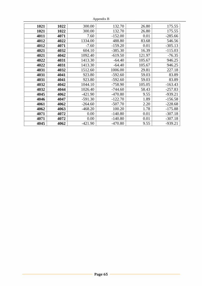
Appendix B
Page 65
1021 1022 300.00 132.70 26.80 175.55
1021 1022 300.00 132.70 26.80 175.55
4011 4071 7.60 -152.00 0.01 -285.66
4012 4022 1334.00 488.80 83.68 546.56
4012 4071 -7.60 -159.20 0.01 -305.13
4021 4032 604.10 -385.30 16.39 -115.03
4021 4042 1092.40 -619.50 121.97 -76.35
4022 4031 1413.30 -64.40 105.67 946.25
4022 4031 1413.30 -64.40 105.67 946.25
4031 4032 1512.60 1006.00 29.81 227.18
4031 4041 923.80 -592.60 59.03 83.89
4031 4041 923.80 -592.60 59.03 83.89
4032 4042 1044.10 -758.90 105.05 -163.43
4032 4044 1026.40 -744.60 58.43 -257.83
4045 4062 -421.90 -470.80 9.55 -939.21
4046 4047 -591.30 -122.70 1.89 -156.58
4061 4062 -264.60 -507.70 2.20 -228.68
4062 4063 -468.20 100.20 1.78 -175.88
4071 4072 0.00 -140.80 0.01 -307.18
4071 4072 0.00 -140.80 0.01 -307.18
4045 4062 -421.90 -470.80 9.55 -939.21

Reference
Page 66
Reference
Reference
[1] Amin, M., „„Challenges in Reliability, Security, Efficiency, and Resilience of Energy
Infrastructure: Toward Smart Self-healing Electric Power Grid‟‟, Power and Energy
Society General Meeting - Conversion and Delivery of Electrical Energy in the 21st
Century, 2008 IEEE , pp.1-5, 20-24 July 2008.
[2] WANG Qing-hong, „„Survey on smart grid research‟‟, Guangxi Electric Power Industry
Investigation Design and Research Institute, 2009 (in Chinese)
[3] U.S.-Canada Power System Outage Task Force, ”August 14th Blackout: Causes and
Recommendations”, 5 April, 2004.
[4] Ekraft System, “Power failure in Eastern Denmark and Southern Sweden on 23
September 2003. Final report on the course of events”, 4 November, 2003.
[5] Commission De Regulation De L‟energie, “Report on the Events of September 28th,
2003 Culminating in the Separation of the Italian Power System from the Other UCTE
Networks”, April 22, 2004.
[6] Massoud Amin, Honeywell, H.W. Sweatt, „„Challenges in Reliability, Security,
Efficiency, and Resilience of Energy Infrastructure: Toward Smart Self-healing Electric
Power Grid‟‟, Power and Energy Society General Meeting - Conversion and Delivery of
Electrical Energy in the 21st Century, pp.1-5, 2008 IEEE, 20-24 July 2008.
[7] Zeinab Noorian, Hadi Hosseini, Mihaela Ulieru, „„An Autonomous Agent-based
Framework for Self-Healing Power Grid‟‟, IEEE, pp. 1983 – 1988, October 11-14th.
2009.
[8] Chongxun Niu, „„the islanding detection and partition of micro grid‟‟, Tianjin University,
master thesis, 1st June 2008 (in Chinese).
[9] K. Moslehi, A.B.R. Kumar, D. Shurtleff, M. Laufenberg, A. Bose, P. Hirsch,
„„Framework for a Self-Healing Power Grid‟‟, Power Engineering Society General
Meeting, 2005. IEEE, Volume 3.1, pp.3027, 12-16 June 2005.
[10] Jian Fu, Mingyu Liu, Chi Feng, „„The discussion about the determination of wind power
farms‟‟, Electric Power Corporation, Volume 23, April 2007 (in Chinese)
[11] Han Shuang, Yang Yongping, Liu Yongqian, „„Study of short-term wind power
prediction method dissertation submitted to north china electric power‟‟, Huabei Electric
Power University, June 2008. (in Chinese)

Reference
Page 67
[12] World Wind Energy Association, „„World Wind Energy Report 2009‟‟, 2009, available
[On line] at http://www.wwindea.org/home/index.php
[13] LEI Ya-zhou, Gordon Lightbody, „„An introduction on wind power grid code and
dynamic simulation‟‟, ESB National Grid Corporation, National University of Ireland
College Cork, December 2005. (in Chinese)
[14] Chun-qi Wang, Qin Yao, Tourxun Yebulayin, „„Study of the power quality problem
caused by large-scale integrated wind farm‟‟, Xin Jiang University, 2 June 2007.
[15] Santiago Grijalva, Scott R. Dahman, Kollin J. Patten, Anthony M. Visnesky, Jr,
„„Large-Scale Integration of Wind Generation Including Network Temporal Security
Analysis‟‟, IEEE, vol. 22, Issue: 1, pp.181-188, 2007.
[16] Powerworld Corporation, „„Strategic Location of Renewable Generation Based on Grid
Reliability‟‟, PowerWorld Users‟ Group Meeting, November 2-3, 2005.
[17] Singh S.N., „„Location of FACTS Devices for Enhancing Power Systems‟ Security‟‟,
2001 Large Engineering Systems Conference on Power Engineering, pp.162-166, 2001.
[18] Baghaee H.R., Vahidi B., Jazebi S., Gharehpetian G.B., Kashefi A., „„Power System
Security Improvement by Using Differential Evolution Algorithm Based FACTS
Allocation‟‟, 2008. Joint International Conference on Power System Technology and
IEEE Power India Conference, pp. 1-6, 12-15 October, 2008.
[19] „„Keeping current reliability standards: meeting national and regional requirements for
electric system reliability‟‟, Bonneville Power Administration, 2003.
[20] Morison K., Lei Wang, Kundur P., „„Power system security assessment‟‟, Power and
Energy Magazine, IEEE, Volume 2, pp. 30 – 39, September-October 2004.
[21] Chakrabarti, Abhijit, Halder, Sunita, „„Power System Analysis: Operation And
Control‟‟, 2006.
[22] Pang, C.K., Prabhakara, F.S., El-Abiad, A.H., Koivo, A.J., „„Security Evaluation in
Power Systems Using Pattern Recognition‟‟, IEEE Transactions on Power Apparatus and
Systems, Volume PAS-93, pp. 969 – 976, May 1974.
[23] Kirschen D.S., „„Do Investments Prevent Blackouts?‟‟, Power Engineering Society
General Meeting, 2007. IEEE, pp.1-5, 24-28 June 2007.
[24] Pang C.K., Prabhakara F.S., El-Abiad A.H., Koivo, A.J., „„Security Evaluation in Power
Systems Using Pattern Recognition‟‟, IEEE Transactions on Power Apparatus and
Systems, Volume PAS-93, pp.969 – 976, May 1974.
[25] Donghyun Choi, Sungjin Lee, Dongho Won, Seungjoo Kim, „„Efficient Secure Group
Communications for SCADA‟‟, IEEE Transactions on Power Delivery, Volume 25, pp.
714-722, April 2010.
[26] D. Choi, H. Kim, D. Won, and S. Kim, “Advanced key management architecture for
secure SCADA communications,” IEEE Trans. Power Del., vol. 24, no. 3, pp. 1154–
1163, Jul. 2009.

Reference
Page 68
[27] C. Beaver, D. Gallup, W. Neumann, and M. Torgerson, „„Key Management for
SCADA‟‟, [Online] Available: http://www.sandia.org/scada/documnets/013252.pdf,
2002.
[28] Leonard L. Grigsby, „„Power System Stability and Control‟‟, May 30, 2007.
[29] Bruce F. Wollenberg, Allen J. Wood, „„Power generation operation and control‟‟, John
Willey&Sons, INC., 1996.
[30] Zhang, B.M., Wang, S.Y., Xiang, N.D., Deng, Y.M., Yan, Z., Zhu, W.G., Pan, M.H.,
Xu, M.L., Wang, J.H., Cui, H.C., „„A security analysis and optimal power flow package
with real-time implementation in Northeast China Power System‟‟, Advances in Power
System Control, Operation and Management, 1993. APSCOM-93., 2nd International
Conference on, Vlome 2, pp. 816-821, 7-10 December 1993.
[31] Di Santo M., Vaccaro A., Villacci D., Zimeo E., „„A distributed architecture for online
power systems security analysis‟‟, IEEE Transactions on Industrial Electronics, Volume
51, pp. 1238 – 1248, December 2004.
[32] Valdez, M.M.T., Agreira, C.I.F., Ferreira, C.M., Barbosa, F.P.M., „„Electrical Power
System security analysis using problem-based learning‟‟, Universities Power Engineering
Conference, 2008. UPEC 2008. 43rd International, pp. 714 – 722, 1-4 September 2008.
[33] Chang, C.S., Chung, T.S., Lo, K.L., „„Application of pattern recognition technique to
power system security analysis and optimization‟‟, IEEE Transactions on Power Systems,
Volume 5, pp. 835 – 841, August 1990.
[34] Balu, N. Bertram, T. Bose, A., Brandwajn V., Cauley G., Curtice D., Fouad A., Fink L.,
Lauby M.G., Wollenberg B.F., Wrubel J.N., „„On-line power system security analysis‟‟,
Proceedings of the IEEE, Volume 80, pp. 262-282, February 1992.
[35] Kundur P., Paserba J. Ajjarapu V. Andersson G., Bose A., Canizares C., Hatziargyriou
N., Hill D., Stankovic A., Taylor C., Van Cutsem T., Vittal, V., „„Definition and
classification of power system stability IEEE/CIGRE joint task force on stability terms
and definitions‟‟, IEEE Transactions on Power Systems, Volume 19, pp. 1387 – 1401,
2004.
[36] Hong Chen, „„Security cost analysis in electricity markets based on voltage security
criteria and web-based implementation‟‟, Thesis requirement for the degree of Doctor of
Philosophy in Electrical and Computer Engineering,Waterloo, Ontario, Canada, 2002.
[37] “NERC Planning Standards,” North American Electric Reliability Council, September
1997.
[38] “Western Systems Coordinating Council Reliability Criteria,” Western Systems
Coordinating Council, March 1997.
[39] “Southwest Power Pool Criteria,” Southwest Power Pool, May 1996.
[40] “MAPP System Design Standards,” Mid-Continent Area Power Pool, December 1994.
Reference
Page 69
[41] “Principles and Guides for Reliability in System Planning,” Southeastern Electric
Reliability Council, April, 1995.
[42] “Principles and Guides for Planning Reliability Bulk Electric Systems,” Florida
Reliability Coordination Council, September, 1996.
[43] “MACC Reliability Principles and Standards,” Mid Atlantic Area Council, March, 1990
[44] “ECAR Reliability Criteria,” East Central Area Reliability Coordination Agreement,
August, 1996.
[45] “Transmission Planning and Guides and the Simulation Testing of the Main Bulk Power
Transmission System to Assess Adequacy and Reliability,” Mid-American
Interconnected Network, November, 1994.
[46] “Criteria for Design and Operation of Interconnected Power Systems,” Northeast Power
Coordinating Council, August, 1995.
[47] McCalley, J. Asgarpoor S., Bertling L., Billinion R., Chao H., Chen J., Endrenyi J.,
Fletcher R., Ford A., Grigg C., Hamoud G., Logan D., Meliopoulos A.P., Ni M., Rau N.,
Salvaderi L., Schilling M., Schlumberger Y., Schneider A., Singh, C., „„Probabilistic
security assessment for power system operations‟‟, Volume 1, pp.212-220, 6-10 June
2004.
[48] SUN Hua-dong, TANG Yong, MA Shi-ying, „„A commentary on Definition and
Classification of Power System Stability‟‟, China Electric Power Research Institute,
Volume 30 No. 17, September 2006.(in Chinese)
[49] „„Power System Stability Regulations‟‟, Department of Energy of Russian Federation,
30 June 2003. [On-line] available: http://www.so-cdu.ru
[50] Fishov A.G., Toutoundaeva D.V., „„Power system stability standardization under
present-day conditions‟‟, IFOST 2007. International Forum on Strategic Technology,
2007, pp. 411 – 415, 3-6 October 2007.
[51] Moslehi K., Kumar R., „„Smart Grid - a reliability perspective‟‟, Innovative Smart Grid
Technologies (ISGT), 2010, pp. 1 – 8, 19-21 January 2010.
[52] CIGRE WG C6.01, “Development of dispersed generation and consequences for power
systems”, July 2003.
[53] Ault G.W., McDonald J.R., Burt G.M., „„Strategic analysis framework for evaluating
distributed generation and utility strategies‟‟, Generation, Transmission and Distribution,
IEE Proceedings, Volume 150, pp. 475-481, 14 July 2003.
[54] „„The wind power targets for Europe‟‟, the European wind energy association
[55] Meyer B., „„Distributed Generation: towards an effective contribution to power system
security‟‟, Power Engineering Society General Meeting, 2007. IEEE, pp. 1 – 6, 24-28
June 2007.
Reference
Page 70
[56] Jun-ping Xu, Neng-sheng Bao, „„Research on dynamic characteristics of wind-gas
turbine generator system‟‟, Shan Tou University.
[57] Chen Lei, XING Zuo-xia, PAN Jian, ZHONG Ming-fang, „„ An overview of large grid-
connected wind generation system status‟‟, Wind Energy Institute, Shenyang University
of Techonology, January 2003. (in Chinese)
[58] Nayeem Rahmat Ullah, „„Wind Power – Added Value for Network Operation‟‟,
Technical Report at Chalmers University of Technology, Technical report no. 2879,
2008.
[59] Abram Perdana, „„Dynamic Models of Wind Turbines, A Contribution towards the
Establishment of Standardized Models of Wind Turbines for Power System Stability
Studies‟‟, Chalmers University of Technology, 2008.
[60] ZHANG Bao-hui, WANG Li-yong, ZHANG Wen-hao, ZHOU De-cai, YAO Feng,
REN Jin-feng, XIE Han, YU Gang-liang, „„Implementation of Power System Security
and Reliability Considering Risk Under Environment of Electricity Market‟‟,
Transmission and Distribution Conference and Exhibition: Asia and Pacific, IEEE/PES,
pp.1-6, 2005.
[61] Santiago Grijalva and Anthony M. Visnesky Jr., „„Spatial Representation of the Effect
of New Generation on Network Security‟‟, IEEE, vol.1, pp.144-149, 18 April 2005.
[62] C. Genesi, P. Marannino, M. Montagna, S. Rossi, I. Siviero, „„Power Flow Based
Indices for the Coordination of Transmission and Generation System Planning‟‟, IEEE
Bucharest,pp.1-7, June 28 2009-July 2 2009.
[63] M. Milligan, D. Lew and D. Corbus, R. Piwko, N. Miller, K. Clark, G. Jordan and L.
Freeman, B. Zavadil, M. Schuerger, „„Large-Scale Wind Integration Studies in the United
States: Preliminary Results‟‟, 8th International Workshop, 14-15 October 2009.
[64] G. B. Ancell and J. W. Clarke, „‟Integration of large scale wind generation in the New
Zealand power system and electricity market‟‟, IEEE, pp.1-6, 20-24 July 2008.
[65] Keith Tynes, Scott R. Dahman, „„Advanced Sensitivity Analysis for Long-Range
Transmission Expansion Planning‟‟, PowerWorld Users‟ Group Meeting, 25-26 October
2007.
[66] R. Piwko, N. Miller, J. Sanchez-Gasca, Y. Xiaoming, D. Renchang, and J. Lyons,
„„Integrating large wind farms into weak power grids with long transmission lines,” in
Proc. IEEE PES T&D Conf. Exhib.: Asia Pac., 2005, pp. 1–7, 15–18 August.
[67] National Grid, available [On line] at http://www.nationalgrid.com/uk/Electricity
[68] Enzo E. Sauma, and Shmuel S. Oren, „„Economic Criteria for Planning Transmission
Investment in Restructured Electricity Markets‟‟, IEEE, Volume 22, pp. 1394 – 1405, 29
October 2007.
[69] Energy balances 2010 and Power Balances 2010/11, Nordel's Balance Group, June
2007,available [On line] at: www.kraftaffarer.se/meralasning/nordelprog.ppt

Reference
Page 71
[70] Hassan, Rabab and Radman, Ghadir, „„Survey on smart grid research‟‟, IEEE, pp.210 –
213, 18-21 March 2010.
[71] Kakimoto, N., Ohnogi, Y., Matsuda, H., Shibuya, H., „„Transient Stability Analysis of
Large-Scale Power System by Lyapunov's Direct Method‟‟, IEEE, Volume PAS-103, pp.
160 – 167, 26 February 2007.
[72] Lj.B. Joci, M. Ribbens-Pavella and D.D. Siljak, Multimachine power system: stability,
decomposition and aggregation. IEEE Trans. Autom. Control, Volume AC-23 (April
1978), pp. 325–332.
[73] Alberto, L.F.C. , Chiang, H.D., „„Theoretical Foundation of CUEP Method for Two-
Time Scale Power System Models‟‟, Power & Energy Society General Meeting, 2009.
PES '09. IEEE, pp. 1 – 9, 2rd October 2009.
[74] U.S.-Canada Power System Outage Task Force, „„Final Report on the August 14, 2003
Blackout in the United States and Canada: Causes and Recommendations‟‟, April 2004,
available [On line] at: https://reports.energy.gov/
[75] J. H. Chow and P. V. Kokotovic, „„Time scale modeling of dynamic networks with
sparse and weak connections‟‟, Volume 90, pp.310-353, January 20, 2006.
[76] Price, W.W., Hargrave, A.W., Hurysz, B.J., Chow, J.H., Hirsch, P.M., „„Large-scale
system testing of a power system dynamic equivalencing program‟‟, IEEE Transactions
on Power Systems, Volume 13 Issue 3, pp. 768 – 774, 6th August 2002
[77] B. Yang, V. Vittal and G. T. Heydt, “Slow Coherency Based Controlled Islanding – A
Demonstration of the Approach on the August 14, 2003 Blackout Scenario”, IEEE Trans.
On Power Systems, vol. 21, No. 4, pp. 1840-1847, November 2006.
[78] Fouad, A., Anderson, P., „„Power System Control and Stability‟‟, IEEE, pp.398 -398,
2002.
[79] Ziguan Zhou, Xiaomin Bai, ShanShan Zhao, Zaihua Li, Jing Xu, Xiaojun Li, „„A New
Islanding Boundary Searching Approach Based on Slow Coherency and Graph
Theoretic‟‟, Natural Computation, 2008. ICNC '08. Fourth International Conference on,
Volume 6, pp.438 – 442, 18-20 October 2008.
[80] R. A. Date and J. H. Chow, „„Aggregation properties of linearized two time-scale power
networks‟‟, IEEE Transaction on Circuits and Systems, Volume 38 Issue 7, pp. 720–730,
July 1991.
[81] Haibo You, Vijay Vittal and Xiaoming Wang, „„Slow Coherency-Based Islanding‟‟
IEEE Transactions on Power Systems, Volume 19 Issue 1, pp. 483 – 491, February 2004.
[82] Luis F. C. Alberto, and H. D. Chiang, „„Controlling Unstable Equilibrium Point Theory
for Stability Assessment of Two-Time Scale Power System Models‟‟, Power and Energy
Society General Meeting - Conversion and Delivery of Electrical Energy in the 21st
Century, 2008 IEEE, pp. 1-9, 20-24 July 2008.

Reference
Page 72
[83] K. Khorasani and M.A. Pai, „„Two time scale decomposition and stability analysis of
power systems‟‟, Control Theory and Applications, IEE Proceedings D, Volume 135
Issue 3, pp. 205 – 212, 11 November 2008.
[84] H. You, V. Vittal, and Z. Yang, “Self-Healing in Power Systems: An Approach using
Islanding and Rate of Frequency Decline-Based Load Shedding,” IEEE Transaction on
Power Systems, Volume.18, No.1, pp 174-181, February 2003.
[85] S. B. Yusof, G. J. Rogers, R. T. H. Alden, “Slow coherency based network partitioning
including load buses,” IEEE Transactions on Power System, Volume. 8, no. 3, pp. 1375–
1382. August 1993.
[86] Mechthild Stoer, Frank Wagner, „„A Simple Min-Cut Algorithm‟‟, Journal of the ACM,
Volume 44 , Issue 4, pp. 585 – 591, 1997.
[87] Sood V.K., Fischer D., Eklund J.M., Brown T., „‟Developing a communication
infrastructure for the Smart Grid‟‟, Electrical Power & Energy Conference (EPEC), 2009
IEEE, pp.1-7, 22-23 October 2009.
[88] X. Wang and V. Vittal, “System Islanding Using Minimal Cutsets with Minimum Net
Flow,” Proceedings of the 2004 IEEE PES Power System Conference and Exposition,
New York, October 2004.
[89] SEZER M.E., and SILJAK D.D., „„Nested &-decompositions and clustering of complex
systems‟‟, Automatica, pp. 321-331, 1986,22.
[90] Kai Sun, Da-Zhong Zheng, Qiang Lu, „„Splitting strategies for islanding operation of
large-scale power systems using OBDD-based methods‟‟, IEEE Transactions on Power
Systems, Volume 18, pp.912 – 923, May 2003.
[91] Lei Ding, Zhencun Pan, Wei Cong, Jianye Pang, „„An Integrated Automatic Control
System for Distributed Generation Hierarchical Islanding‟‟, PowerCon 2006.
International Conference on Power System Technology, 2006., pp.1 – 6, 22-26 October
2006.
[92] S.A.Taher and H.Besharat, „„Transmission congestion management by determining
optimal location of FACTS devices in deregulated power systems‟‟, American Journal of
Applied Sciences, March 2008.
[93] Zuyi Li, “Fundamentals of Power System Economics‟‟, Power and Energy Magazine,
IEEE, Volume 4, Issue 4,pp. 76 – 78, 17 July 2006.
[94] Istardi, D., Abba-Aliyu, S., Bergqvist, A., Rouch, N. Abdalrahman, A.M., Le Anh
Tuan, Bertling, L. „„Understanding power system voltage collapses using ARISTO:
Effects of protection‟‟, PowerTech, 2009 IEEE Bucharest, pp.1-7, June 28 2009-July 2
2009.
[95] Ng, C.H., Li Ran, Bumby, J., „„Unbalanced-Grid-Fault Ride-Through Control for a
Wind Turbine Inverter‟‟, IEEE Transactions on Industry Applications, Volume 44, pp.
845-856, May-June 2008.