power quality analysis and automatic intelligent …
TRANSCRIPT

POWER QUALITY ANALYSIS AND AUTOMATIC INTELLIGENT
CONTROL STRATEGY FOR SOLAR PV MICROGRID
by
ARANGARAJAN VINAYAGAM
(BTECH – Electrical and Electronics Engineering)
Submitted in fulfillment of the requirements for the degree of
Doctor of Philosophy
Deakin University
August 2017


Acknowledgements
I would like to express sincere gratitude and appreciation to Prof. Alex Stojcevski,
who has given me the great opportunity with his full support to do my PhD at Deakin
University, Australia. He has provided me with the guidance, advice, and motivation
during my entire research.
I am thankful to Dr. Sui Yang Khoo, who agreed to supervise my research work at
the end of my candidature. I would like to appreciate his patience, motivation,
attitude, and flexibility of the approach with regular discussion of key points in the
final stage of my research. I also extend my thanks to associate supervisor Assoc.
Prof. Aman Than Oo for his valuable suggestions and guidance throughout my
research.
I would like to take this opportunity to thank the management, all faculties, technical
and administrative staffs of Deakin University, and all the colleagues from my
research group for their support. I would like to acknowledge the support of Mr Tim
Moore (CSIRO Renewal Energy Integration Facility, Newcastle, Australia), who has
provided me the access to use the facility and guidance support for doing the
experimental analysis.
Last but not least, many thanks to my parents and my wife Geetha, who have given
continual support and encouragement throughout my journey of PhD. Also, I would
like to extend thanks to my co-brother Dr.Jaideep Chandran, his wife Lavanya and
their son Ishan, for their hospitality, love and support.
ABSTRACT
In this thesis, other than the THD, the effect of multiple scenarios on the PQ factors
like VUF, variation in the power, voltage and frequency level in the PV based MG
network were analyzed through the simulation and experimental approach.
Simulation results using PSS SINCAL indicated that PV penetration level in the
presence of different types of loads, unbalanced load/ PV generation and cloud effect
could significantly affect the PQ factors in the MG network. Experiments on a real-
time MG also indicated the effect of various scenarios on the PQ factors, however, in
the presence of real cloud effect.
A co-ordinated power management/power sharing control was implemented along
with the use of grid support grid forming (GsGfm) type VSI for PV and battery (DG
units) of the MATLAB-SIMULINK MG model. The variations in power, voltage
and frequency were found to be higher for the islanded mode than the on-grid mode
of MG operation. Thus, a PSO based optimization algorithm along with the proposed
cost function was applied to the GsGfm type VSI of the DG units in the same
MATLAB-SIMULINK MG model to obtain the optimized power flow and further
minimize the variation in reactive power and frequency level. The islanded MG
network implemented with the PSO algorithm with the proposed cost function
showed superior performance in comparison to the results before the optimization.
Penalty function incorporated into the cost function ensured frequency variation
within the acceptable operating range as per the standard limit.

TABLE OF CONTENTS
ABSTRACT............................................................................................................................................................... IV
LIST OF FIGURES .................................................................................................................................................... IX
LIST OF TABL ES ..................................................................................................................................................... XII
LIST OF PUBLICATIONS ....................................................................................................................................XVIII
CHAPTER 1 ............................................................................................................................................................... 1
INTRODUCTION ...................................................................................................................................................... 1
1.1 BACKGROUND ............................................................................................................................................. 1 1.2 PROBLEM STATEMENT.............................................................................................................................. 3 1.3 OBJECTIVES ................................................................................................................................................ 4 1.4 SCOPE O F THIS THESIS .............................................................................................................................. 5 1.5 OUTLINE ...................................................................................................................................................... 7
CHAPTER 2 ............................................................................................................................................................... 9
LITERATURE REVIEW ............................................................................................................................................. 9
2.1 INTRO DUCTIO N........................................................................................................................................... 9 2.2 CO NCEPT O F MG ....................................................................................................................................... 9 2.3 MG ARCHITECTURE CO MPONENTS...................................................................................................... 10 2.4 MG TECHNICAL CHALLENGES ............................................................................................................. 11 2.5 PV BASED MG WITH INTEGRATIO N O F BATTERY STO RAGE FACILITY ........................................ 16
2.5.1 Solar PV cell ..................................................................................................................................... 16 2.5.1.1 PV cell characteristics curve .......................................................................................................17
2.5.2 Energy Storage (ES) ....................................................................................................................... 19 2.6 VO LTAGE SO URCE INVERTER (VS I).................................................................................................... 20
2.6.1 Synchronous Reference Frame (SRF) Theory for VSI control application....................... 21 2.6.2 Equivalent circuit of VSI ............................................................................................................... 22 2.6.3 Types of VSI control configuration ............................................................................................. 23
2.6.3.1 Generic control configuration of the GsGfm type VSI ............................................................26 2.7 POWER MANAGEMENT AND POWER SHARING CONTRO L ................................................................ 33
2.7.1 Co-ordinated power management control – previous research works ................................. 33 2.7.2 Power sharing control – previous research works ................................................................... 35
2.8 NEED FO R OPTIMIZATIO N TECHNIQUES IN THE MG NETWO RK .................................................... 36 2.8.1 Particle Swarm Optimization (PSO) algorithm......................................................................... 37
2.8.1.1 Basic rules of PSO Algorithm .....................................................................................................38 2.8.1.2 Cost function ................................................................................................................................41
2.8.2 Previous research works on the use of PSO optimization in the MG network .................. 43
2.9 SUMMARY .................................................................................................................................................. 45
CHAPTER 3 ............................................................................................................................................................. 47
ANALYSIS OF POWER QUALITY IMPACTS IN A TYPICAL MG NETWORK .................................................. 47

3.1 INTRO DUCTIO N......................................................................................................................................... 47 3.2 DEVELO PMENT O F THE MG POWER SYSTEM MODEL ...................................................................... 48 3.3 METHOD O F ANALYSIS ........................................................................................................................... 52
3.3.1 Load flow analysis ........................................................................................................................... 52 3.3.1.1 Power and voltage variation .......................................................................................................53
3.3.2 THD analysis .................................................................................................................................... 54 3.3.2.1 Total Harmonic Distortion (THD) .............................................................................................54
3.3.3 Unbalance voltage analysis ........................................................................................................... 56 3.3.3.1 Unbalance voltage ........................................................................................................................56
3.4 RESULTS AND DISCUSSION..................................................................................................................... 57 3.4.1 Power variation-Results discussion ............................................................................................. 58 3.4.2 Voltage variation-Results discussion........................................................................................... 60 3.4.3 Current and voltage THD-Results discussion ........................................................................... 61
3.4.3.1 THD at LV bus node N7..............................................................................................................63 3.4.3.2 THD at LV bus node N9..............................................................................................................64 3.4.3.3 THD at LV bus node N10............................................................................................................65
3.4.4 Unbalance Voltage-Results discussion ....................................................................................... 66
3.5 CO NCLUSION............................................................................................................................................. 68
CHAPTER 4 ............................................................................................................................................................. 71
EXPERIMENTAL ANALYSIS OF POWER QUALITY IN A REAL MG NETWORK ............................................ 71
4.1 INTRO DUCTIO N......................................................................................................................................... 71 4.2 MG NETWO RK CONFIGURATIO N ......................................................................................................... 72 4.3 DESCRIPTION O F PQ ISSUES.................................................................................................................. 75
4.3.1 Frequency and Voltage Variation................................................................................................ 75 4.3.2 Unbalance Voltage and Neutral Current ................................................................................... 76 4.3.3 Total Harmonic Distortion (THD) ............................................................................................... 77
4.4 METHOD O F ANALYSIS ........................................................................................................................... 78 4.4.1 Voltage and frequency variation/deviation was analysed with the following conditions:
....................................................................................................................................................................... 78 4.4.2 Unbalance Voltage and Neutral Current analysis ................................................................... 80 4.4.3 THD analysis .................................................................................................................................... 80
4.5 RESULTS AND DISCUSSION..................................................................................................................... 80 4.5.1 Results of Voltage and frequency variation/deviation ............................................................. 81
4.5.1.1 Stepped Variation of PV Power with Constant Load: On-Grid Mode ..................................81 4.5.1.2 Actual PV Power Variation with the constant Load: Off-Grid Mode....................................84 4.5.1.3 Frequent Power Variation and Load Variation: On-Grid ......................................................87
4.5.2 Results of Unbalance Voltage and Neutral Current level ...................................................... 92 4.5.3 Results of Total Harmonic Distortion (THD) ........................................................................... 95
4.6 CO NCLUSION............................................................................................................................................. 99
CHAPTER 5 ...........................................................................................................................................................101
POWER MANAGEMENT AND POWER SHARING CONTROL OF SOLAR PV MG .....................................101
5.1 INTRO DUCTIO N.......................................................................................................................................101 5.2 MG MO DEL CO NFIGURATION ............................................................................................................102
5.2.1 Solar PV unit and DC Power converter ....................................................................................104 5.2.2 Battery storage and Bi-directional DC Power converter.......................................................105

5.2.3 Control configuration of GsGfm type VSI for the developed MG model ..........................107
5.2.3.1 Modified droop control loop (for LV network) ......................................................................109 5.2.3.2 Virtual impedance (resistor) control loop ...............................................................................110 5.2.3.3 Voltage and current control loop of VSI .................................................................................111
5.3 POWER MANAGEMENT CONTRO L STRATEGIES ...............................................................................113 5.3.1 PV Power Management (on-grid) ..............................................................................................114 5.3.2 Battery power management with inclusion of SOC control (on-grid) ...............................115 5.3.3 Power management of PV units (off-grid) ...............................................................................119 5.3.4 Battery power management (off-grid).......................................................................................119
5.3.4.1 SOC control and Load power management (off-grid) ...........................................................122 5.4 MO DEL ANALYSIS AND RESULTS.........................................................................................................123
5.4.1 On-grid mode Analysis .................................................................................................................123 5.4.1.1 Results and Discussion (On-grid) .............................................................................................124
5.4.2 Off-grid mode analysis .................................................................................................................128 5.4.2.1 Results and Discussion (Off-grid).............................................................................................129 5.4.2.2 Minimum SOC level (Off-grid) ................................................................................................131
5.4.3 On-grid to Off-grid transition mode Analysis .........................................................................133 5.4.3.1 Results and discussion (On-grid to Off-grid) ..........................................................................134
5.4.4 Total Harmonic Distortion (THD) (Results and discussion) ...............................................136 5.5 CO NCLUSION...........................................................................................................................................137
CHAPTER 6 ...........................................................................................................................................................138
INTELLIGENT CONTROL STRATEGY.................................................................................................................138
6.1 INTRO DUCTIO N.......................................................................................................................................138 6.2 METHOD O F OPTIMIZATIO N ................................................................................................................139
6.2.1 Formulation of the cost function ...............................................................................................141 6.2.2 MATLAB M-file codes with Process steps of PSO .................................................................144 6.2.3 Settings of PSO parameters .........................................................................................................146
6.3 SIMULATIO N, ANALYSIS AND RESULTS DISCUSSION .......................................................................148 6.3.1 Power flow optimization ...............................................................................................................149 6.3.2 Active and Reactive power optimization ...................................................................................151
6.3.2.1 Performance of DG inverters control (at initial state) ...........................................................154 6.3.2.2 Steady state response (Active power) of the DG inverters (At different loads) ...................155 6.3.2.3 Steady state response (Reactive power) of DG inverters (at high demand) .........................156 6.3.2.4 Reactive power variation from DG units (during load change condition) ...........................157
6.3.3 Minimization of frequency variation.........................................................................................158
6.4 DISCUSSIO N .............................................................................................................................................161 6.5 CO NCLUSION...........................................................................................................................................163
CHAPTER 7 ...........................................................................................................................................................165
CONCLUSION AND FUTURE WORK ................................................................................................................165
7.1 MAIN O UTCOMES ...................................................................................................................................165 7.2 CO NTRIBUTIO NS OF THE TH ESIS.........................................................................................................166 7.3 FUTURE WORKS ......................................................................................................................................168
REFERENCES ........................................................................................................................................................170
APPENDIX ............................................................................................................................................................180

APPENDIX A ........................................................................................................................................................180
A1 FEATURES OF PSS SINCAL POWER SIMULATION SOFTWARE.............................................................180
A1.1 DESCRIPTIO N O F POWER SYSTEM NETWORK MODEL IN PSS SINCAL ..................................180 A1.1.1 Network Elements in PSS SINCAL ........................................................................................181 A1.1.2 AC In-feeder ................................................................................................................................182 A1.1.3 Transformer .................................................................................................................................183 A1.1.4 Line or conductor .......................................................................................................................183 A1.1.5 Load ...............................................................................................................................................184 A1.1.6 DC In-feeder ................................................................................................................................185 A1.1.7 Synchronous Machine element ...............................................................................................186 A1.1.8 Node/Bus bar ...............................................................................................................................187
A1.2 SELECTIO N O F THE CALCULATIO N METHODS ..............................................................................188 A1.2.1 Settings for LF calculation.......................................................................................................188 A1.2.2 Settings for the unbalanced LF calculation .........................................................................189 A1.2.3 Settings for the Harmonics calculation .................................................................................191
A1.3 MAIN INPUT DATA FO R THE NETWO RK MODEL............................................................................192 A1.3.1 Load data for daily load profile ...............................................................................................192 A1.3.2 Solar data for daily solar profile .............................................................................................193 A1.3.3 Current harmonic data for PV inverters and non-linear load..........................................193
APPENDIX B.........................................................................................................................................................195
B1 FORMULATION OF ERROR SIGNALS FOR OPTIMIZATION ...................................................................195

LIST OF FIGURES
FIGURE 1 MARKET SHARE OF MG CAPACITY IN WORLDWIDE .........................................................................2 FIGURE 2 MG ARCHITECTURE .............................................................................................................................11 FIGURE 3 I-V CHARACTERISTICS OF PV CELL ..................................................................................................18 FIGURE 4 DC BOOST CONVERTER........................................................................................................................19 FIGURE 5 BASIC SYSTEM OF POWER INVERTER ................................................................................................23 FIGURE 6 (A) GRID-FORMING; (B) GRID-FEEDING; (C) GRID-SUPPORT GRID-FEEDING;(D) GRID-SUPPORT
GRID-FORMING TYPE INVERTER .................24 FIGURE 7 GSGFM CONTROL OF POWER INVERTER ...........................................................................................26 FIGURE 8 EQUIVALENT CIRCUIT OF DISTRIBUTION POWER NETWORK [69]...................................................27 FIGURE 9 PSO PROCESS FLOW CHART ...............................................................................................................41 FIGURE 10 SCHEMATIC DIAGRAM OF MG POWER SYSTEM MODEL ................................................................49 FIGURE 11 TYPICAL DAILY SOLAR PROFILE WITH SOLAR DISTURBANCE.......................................................53 FIGURE 12 PV POWER VARIATION DURING SOLAR DISTURBANCE..................................................................58 FIGURE 13 POWER FLOW FROM GENERATION SIDE (GRID/DG UNIT ).............................................................59 FIGURE 14 POWER VARIATION DURING SOLAR DISTURBANCE (GRID/DIESEL GENERATOR) ......................59 FIGURE 15 VOLTAGE LEVEL OF ALL THREE PHASES .........................................................................................61 FIGURE 16 VOLTAGE VARIATION (DURING SOLAR DISTURBANCE) ................................................................61 FIGURE 17 INTEGRATION OF PV WITH DIFFERENT TYPES OF LOADS AT LV BUS NODES .............................62 FIGURE 18 HARMONICS CURRENT CURVE OF TYPICAL PV INVERTER ............................................................62 FIGURE 19 HARMONICS CURRENT CURVE OF NON-LINEAR LOAD ...................................................................63 FIGURE 20 PV WITH LINEAR LOAD AT LV BUS NODE N7.................................................................................64 FIGURE 21 PV WITH NON-LINEAR LOAD AT LV BUS NODE N9 .......................................................................65 FIGURE 22 PV WITH COMPOSITE LOAD AT LV BUS NODE N10 .......................................................................66 FIGURE 23 UNEVEN DISTRIBUTION OF THE LOADS AND PV UNITS .................................................................67 FIGURE 24 UNBALANCE VOLTAGE PROFILE AT LV BUS NODE N8..................................................................67 FIGURE 25 UNBALANCE VOLTAGE LEVEL AT LV BUS NODE N8.....................................................................68 FIGURE 26 MG NETWORK CONFIGURATION (CSIRO REIF) [116] ................................................................73 FIGURE 27 MG CONFIGURATION FOR VOLTAGE AND FREQUENCY ANALYSIS (ON-GRID) ...........................82 FIGURE 28 PV POWER VERSUS LOAD POWER (ON-GRID) .................................................................................82 FIGURE 29 FREQUENCY LEVEL (POWER VARIATION WITH CONSTANT LOAD, ON-GRID) .............................83 FIGURE 30 VOLTAGE LEVEL (POWER VARIATION WITH CONSTANT LOAD, ON-GRID)..................................83 FIGURE 31 MG CONFIGURATION FOR VOLTAGE AND FREQUENCY ANALYSIS (OFF-GRID)..........................84 FIGURE 32 POWER LEVEL OF PV (CONSTANT LOAD, OFF-GRID) .....................................................................85 FIGURE 33 POWER LEVEL OF MT GENERATOR (CONSTANT LOAD, OFF-GRID) .............................................85 FIGURE 34 POWER LEVEL OF PV, MT, AND LOAD (CONSTANT LOAD, OFF-GRID) ........................................86 FIGURE 35 FREQUENCY VARIATION (CONSTANT LOAD, OFF-GRID MODE)....................................................86 FIGURE 36 VOLTAGE VARIATION (CONSTANT LOAD, OFF-GRID MODE).........................................................87 FIGURE 37 MG CONFIGURATION (FREQUENT POWER AND LOAD VARIATION (ON-GRID)............................88 FIGURE 38 TYPICAL SOLAR PROFILE...................................................................................................................88 FIGURE 39 TYPICAL LOAD PROFILE.....................................................................................................................89 FIGURE 40 ACTIVE POWER OF MICRO TURBINE AND LOAD ............................................................................89 FIGURE 41 FREQUENCY LEVEL AT PCC (VARYING LOAD, ON-GRID) .............................................................90 FIGURE 42 VOLTAGE LEVEL AT PCC (VARYING LOAD, ON-GRID)..................................................................90 FIGURE 43 MG CONFIGURATION WITH UNEVEN DISTRIBUTION OF LOADS AND PV ....................................92 FIGURE 44 UNBALANCED PV POWER VARIATION.............................................................................................93 FIGURE 45 POWER LEVEL OF UNBALANCED LOAD............................................................................................93 FIGURE 46 VOLTAGE LEVEL AT LV NETWORK..................................................................................................93 FIGURE 47 MG CONFIGURATION DURING HARMONICS ANALYSIS .................................................................95

FIGURE 48 PV POWER PROFILE ............................................................................................................................96 FIGURE 49 CURRENT THD AT DIFFERENT LEVEL OF PV POWER ....................................................................97 FIGURE 50 VOLTAGE THD AT DIFFERENT LEVEL OF PV POWER....................................................................97 FIGURE 51 CURRENT THD OF ODD HARMONICS ...............................................................................................97 FIGURE 52 TYPICAL CONFIGURATION OF MG MODEL....................................................................................103 FIGURE 53 PV UNIT PV CURVE (POWER VERSUS VOLTAGE) ........................................................................104 FIGURE 54 PV UNIT I-V CURVE .........................................................................................................................105 FIGURE 55 BATTERY DISCHARGE CURVE .........................................................................................................106 FIGURE 56 OVERALL CONTROL CONFIGURATION OF VSI[88,89] .................................................................108 FIGURE 57 POWER CALCULATION BLOCK WITH MODIFIED DROOP CONTROL .............................................108 FIGURE 58 CONFIGURATION OF VOLTAGE AND CURRENT CONT ROL............................................................108 FIGURE 59 PV POWER MANAGEMENT (ON-GRID) ..........................................................................................114 FIGURE 60 ACTIVE POWER MANAGEMENT OF BATTERY (ON-GRID)............................................................116 FIGURE 61 REACTIVE POWER MANAGEMENT OF BATTERY (ON-GRID) .......................................................117 FIGURE 62 FLOW CHART FOR POWER MANAGEMENT OF BATTERY (ON-GRID) ...........................................117 FIGURE 63 LOOK-UP TABLE FOR BATTERY DISCHARGE (2ND LEVEL) ..........................................................118 FIGURE 64 ACTIVE POWER MANAGEMENT OF BATTERY (OFF-GRID)............................................................121 FIGURE 65 REACTIVE POWER MANAGEMENT OF BATTERY (OFF-GRID)......................................................121 FIGURE 66 FLOW CHART FOR POWER MANAGEMENT OF BATTERY (OFF-GRID) .........................................122 FIGURE 67 POWER SHARING AMONG T HE POWER SOURCES AND LOAD (ON-GRID) ....................................125 FIGURE 68 VOLTAGE AND FREQUENCY LEVEL (ON-GRID) ............................................................................127 FIGURE 69 POWER SHARING AMONG SOURCES AND LOAD (OFF-GRID)........................................................129 FIGURE 70 VOLTAGE AND FREQUENCY LEVEL (OFF-GRID) ...........................................................................130 FIGURE 71 SOC AND LOAD MANAGEMENT CONTROL AT MINIMUM SOC LEVEL .......................................132 FIGURE 72 POWER AND VOLTAGE/FREQUENCY LEVEL DURING TRANSITION (ON-GRID TO OFF-GRID) ...134 FIGURE 73 (A) VOLTAGE THD; (B) CURRENT THD .......................................................................................136 FIGURE 74 SINGLE LINE DIAGRAM OF THE MG WITH THE PSO APPLICATION ............................................139 FIGURE 75 IMPLEMENTATION OF PSO CONTROL ALGORITHM ......................................................................144 FIGURE 76 CONVERGENCE CURVE ....................................................................................................................148 FIGURE 77 ACTIVE POWER AT DIFFERENT LOAD CONDITIONS (AFTER OPTIMIZATION) ............................150 FIGURE 78 REACTIVE POWER AT DIFFERENT LOAD CONDITIONS (AFTER OPTIMIZATION)........................150 FIGURE 79 CURRENT COMPONENTS (ID, IQ) OF THE DG INVERTERS ............................................................151 FIGURE 80 CURRENT COMPONENTS (ID, IQ) OF THE DG INVERTERS ............................................................152 FIGURE 81 ACTIVE POWER OF THE PV UNITS AND BATTERY ST ORAGE (AFTER OPTIMIZATION) .............152 FIGURE 82 REACTIVE POWER OF PV UNITS AND BATTERY ST ORAGE (BEFORE OPTIMIZATION) ..............153 FIGURE 83 REACTIVE POWER OF PV UNITS AND BATTERY STORAGE (AFTER OPTIMIZATION) ................153 FIGURE 84 FREQUENCY VARIATION DURING LOAD CHANGE (BEFORE OPTIMIZATION) ............................159 FIGURE 85 FREQUENCY VARIATION DURING LOAD CHANGE (AFTER OPTIMIZATION)...............................159 FIGURE 86 WORK SPACE TOOL ARRANGEMENT OF PSS SINCAL................................................................181 FIGURE 87 A TYPICAL SIMPLE NETWORK .........................................................................................................182 FIGURE 88 SETTINGS OF IN-FEEDER BLOCK .....................................................................................................182 FIGURE 89 SETTINGS OF THE TRANSFORMER ELEMENT.................................................................................183 FIGURE 90 SETTINGS OF LINE ELEMENT BLOCK ..............................................................................................184 FIGURE 91 SETTINGS OF THE LOAD ELEMENT .................................................................................................185 FIGURE 92 ELEMENTS OF DC IN-FEEDER BLOCK ............................................................................................185 FIGURE 93 SETTINGS OF PV ELEMENT WITH INVERTER CONFIGURATION ...................................................186 FIGURE 94 SETTINGS OF THE POWER UNIT GENERATOR ................................................................................187 FIGURE 95 SETTINGS FOR THE LF CALCULATION ...........................................................................................189 FIGURE 96 SETTINGS FOR THE UNBALANCED LF CALCULATION ..................................................................190 FIGURE 97 SETTINGS OF THE LOAD ELEMENT CONNECTION..........................................................................190 FIGURE 98 SETTINGS OF THE HARMONICS CALCULATION .............................................................................191 FIGURE 99 TYPICAL DAILY LOAD PROFILE WITH INPUT SETTINGS OF LOAD DATA.....................................192

FIGURE 100 TYPICAL DAILY SOLAR PROFILE (NORMAL SOLAR VERSUS SOLAR DISTURBANCE) ..............193 FIGURE 101 HARMONICS CURRENT DATA AND CURRENT CURVE OF PV INVERTER ...................................194 FIGURE 102 MAIN CONTROL CIRCUIT OF VSI..................................................................................................195 FIGURE 103 VOLTAGE (VD) CONTROL LOOP WITH FORMULATION OF ERROR SIGNAL EA ........................196 FIGURE 104 VOLTAGE (VQ) CONTROL LOOP WITH FORMULATION OF ERROR SIGNAL EB ........................196 FIGURE 105 FORMULATION OF FREQUENCY ERROR SIGNAL EF ....................................................................197 FIGURE 106 MATLAB WORK SPACE SIGNALS (OPTIMIZATION).....................................................................197

LIST OF TABLES
TABLE 1 SPECIFICATION OF GRID SOURCE AND DIESEL GENERATOR .............................................................................. 50 TABLE 2 SPECIFICATION OF DG SOURCES .................................................................................................................... 51 TABLE 3 SPECIFICATION OF TRANSFORMERS................................................................................................................ 51 TABLE 4 SPECIFICATION OF LOADS .............................................................................................................................. 51 TABLE 5 SPECIFICATION OF LINE CONDUCTOR (11 KV) ................................................................................................ 51 TABLE 6 RESULTS OF POWER VARIATION AND VOLTAGE VARIATION .............................................................................. 57 TABLE 7 RESULTS OF THD AND UNBALANCE VOLTAGE LEVEL ....................................................................................... 58 TABLE 8 ACCEPTABLE RANGE OF FREQUENCY LEVEL AS PER NETWORK STANDARD (NEM) [110] .................................. 76 TABLE 9 ACCEPTABLE RANGE OF VOLTAGE LEVEL AS PER AS 60038 STANDARD [110].................................................. 76 TABLE 10 COMPATIBILITY OF UNBALANCE VOLTAGE LEVEL IN LV NETWORK [111]........................................................ 77 TABLE 11 CURRENT THD LIMIT AS PER THE AS 4777 STANDARD [110] ...................................................................... 78 TABLE 12 FREQUENCY VARIATION (HZ) ...................................................................................................................... 91 TABLE 13 VOLTAGE VARIATION (%)............................................................................................................................ 91 TABLE 14 OVERALL RESULTS OF VUF AND NEUTRAL CURRENT (IN) .............................................................................. 94 TABLE 15 RESULTS OF THD LEVEL AT DIFFERENT PV POWER LEVEL .............................................................................. 98 TABLE 16 RESULTS OF ODD HARMONICS AT DIFFERENT PV POWER LEVEL ..................................................................... 98 TABLE 17 DETAILS OF DC EQUIPMENT .....................................................................................................................103 TABLE 18 DETAILS OF LV LOAD AND FEEDER .............................................................................................................103 TABLE 19 DETAILS OF AC EQUIPMENT .....................................................................................................................104 TABLE 20 INVERTER CONTROL AND SYSTEM PARAMETERS ..........................................................................................112 TABLE 21 FREQUENCY AND VOLTAGE LEVEL (ON-GRID)..............................................................................................127 TABLE 22 FREQUENCY AND VOLTAGE LEVEL (OFF-GRID) .............................................................................................131 TABLE 23 FREQUENCY AND VOLTAGE LEVEL (ON-GRID TO OFF-GRID) ..........................................................................135 TABLE 24 MATLAB-M FILE CODES FOR EXECUTION ..................................................................................................144 TABLE 25 PROCESS STEPS OF PROPOSED PSO ALGORITHM ........................................................................................145 TABLE 26 MAIN PARAMETERS OF PSO .....................................................................................................................147 TABLE 27 OPTIMIZED CONTROL PARAMETERS OF THE INVERTER VOLTAGE CONTROLLER ..............................................148 TABLE 28 PERFORMANCE OF THE DG INVERTERS (AT INITIAL STATE) ..........................................................................155 TABLE 29 STEADY STATE RESPONSE (ACTIVE POWER) OF DG INVERTERS (AT DIFFERENT LOADS) ..................................156 TABLE 30 STEADY STATE RESPONSE (REACTIVE POWER) OF DG INVERTERS (HIGH DEMAND) .......................................157 TABLE 31 REACTIVE POWER VARIATION (DURING LOAD CHANGE CONDITIONS) ...........................................................157 TABLE 32 FREQUENCY LEVEL AND FREQUENCY VARIATION (BEFORE AND AFTER OPTIMIZATION) ..................................160 TABLE 33 FREQUENCY LEVEL AS PER THE STANDARD (BEFORE AND AFTER OPTIMIZATION)...........................................160 TABLE 34 DETAILS OF TYPICAL NETWORK ELEMENTS ..................................................................................................181

List of Abbreviations
AC Alternating Current
AEMO Australian Energy Market Operator
Ah Ampere hour
AI Artificial Intelligence
ATO Anti-colony Optimization
BMS Battery Management System
CAES Compressed Air Energy Storage
CC Central Controller
CCM Current Control Mode
CHP Combined Heat and Power
CSIRO Commonwealth Scientific and Industrial Research
Organization
DAQ Data Acquisition
DC Direct Current
DE Differential Evaluation
DFIG Double fed Induction Generator
DG Distributed Generation
EOM Energy and Operation Management

ES Energy Storage
FES Flywheel Energy Storage
FQB Frequency-Reactive Power Boost
GA Genetic Algorithm
GHG Green House Gas
GsGfd Grid-support Grid-feeding
GsGfm Grid-support Grid-forming
HC Hill Climb
HRES Hybrid Renewable Energy System
HV High Voltage
IAE Integral Absolute Error
IC Incremental Conductance
IEC International Electro technical Commission
IEEE Institute of Electrical and Electronics Engineers
IGBT Insulated Gate Bipolar Transistor
ISE Integral Square Error
ITAE Integral Time Absolute Error
ITSE Integral Time Square Error

KVA Kilo Volt Ampere
KVAR Kilo Volt Ampere Reactive
KW Kilo Watt
LF Load Flow
LPF Low Pass Filter
LPSP Loss of Power Supply Probability
LV Low Voltage
MAS Multi Agent System
MG Microgrid
MGCC Microgrid Central Controller
MOPSO Multi Objective Particle Swarm Optimization
MOSFET Metal Oxide Semiconductor Field Effect Transistor
MPPT Maximum Power Point Tracking
MPSO Modified Particle Swarm Optimization
MT Micro Turbine
MV Medium Voltage
NEMA National Electrical and Manufacturers Association
NEM National Electricity Market

P&O Perturb and Observe
PCC Point of Common Coupling
PE Power Electronics
PHES Pumped Hydro Energy Storage
PL Active Power Load
PLL Phase Locked Loop
PMSG Permanent Magnet Synchronous Generator
PQ Power Quality
PSO Particle Swarm Optimization
PSS SINCAL Power System Simulator/Siemens Network Calculation
PV Photovoltaic
PWM Pulse Width Modulation
QL Reactive Power Load
RE Renewable Energy
REIF Renewable Energy Integration Facility
RTDS Real-Time Digital Simulator
RVFC Real time Voltage and Frequency Compensation Strategy
SC Super Capacitor

SCADA Supervisory Control and Data Acquisition
SDS Stochastic Diffusion Search
SMES Super Magnetic Energy Storage
SOC State of Charge
SOH State of Health
SPOF Single Point of Failure
SRF Synchronous Reference Frame
STC Standard Test Condition
TES Thermal Energy Storage
THD Total Harmonic Distortion
THFF Telephone High Frequency Factor
UPS Uninterrupted Power Supply
VCM Voltage Control Mode
VDC Voltage Droop Control
VNR Virtual Negative Resistor
VPD Voltage Active Power droop
VSI Voltage Source Inverter
VUF Unbalance Voltage Factor

LIST OF PUBLICATIONS
BOOK CHAPTER
1. Arangarajan Vinayagam, Aman Than Oo, Jaideep Chandran, Alex
Stojcevski, “Role of Energy Storage in the Power System Network”, NOVA
Science Publishers Inc. USA, Chapter 13, PP.201-225-2015.
JOURNAL PUBLICATIONS
2. Arangarajan Vinayagam, Ahmad Abu Alqusan, KSV Swarna, Sui Yang
Khoo, Aman Than Oo, Alex Stojcevski, “Intelligent Control Strategy in the
Islanded Network of a Solar PV Microgrid”, submitted to the Journal of
“Electric Power Systems Research” (Elsevier).
3. Arangarajan Vinayagam, KSV Swarna, Sui Yang Khoo, Aman Than Oo,
Alex Stojcevski, “PV based Microgrid with Grid-Supporting Grid-forming
Inverter control (Simulation and Analysis)”, Smart Grid and Renewable
Energy, Scientific Research Publishing Inc. Volume 8 (1), PP.1-30, 2017.
4. Arangarajan Vinayagam, KSV Swarna, Sui Yang Khoo, Alex Stojcevski,
“Power Quality Analysis in Microgrid: An Experimental Approach”, Journal
of Power and Energy Engineering, Scientific Research Publishing Inc.
Volume 4 (4), PP.17-34, 2016.
5. Arangarajan Vinayagam, GM Shafiullah, Aman Than Oo, Alex Stojcevski,
“Potentialities of Renewable Energy in Victoria, Australia”, Journal of
Energy and Power Engineering, David Publishing Company-USA, Volume 8
(6), PP.990-1001, 2014.

CONFERENCE PUBLICATIONS
6. Arangarajan Vinayagam, Asma Aziz, KSV Swarna, Sui Yang Khoo, Alex
Stojcevski, “Power Quality Impacts in a Typical Microgrid”, International
Conference on Sustainable Energy and Environmental Engineering (SEEE),
Bangkok, Thailand-2015.
7. KSV Swarna, Arangarajan Vinayagam, Sui Yang Khoo, Alex Stojcevski,
“Impacts of integration of wind and solar PV in a typical power network”,
International Conference on Sustainable Energy and Environmental
Engineering (SEEE), Bangkok, Thailand-2015.
8. Arangarajan Vinayagam, KSV Swarna, Aman Than Oo, Mohammad T
Arif, Alex Stojcevski, “Impact Analysis study in a Typical Solar PV
Microgrid Power system”, International Conference on Power Electronics
and Energy Engineering (PEEE), Hong Kong-2015.
9. KSV Swarna, Arangarajan Vinayagam, Aman Than Oo, Alex Stojcevski,
“Performance Analysis of a Grid-connected PV system in LV distribution
Network”, International Conference on Power Electronics and Energy
Engineering (PEEE), Hong Kong-2015.
10. Asma Aziz, Aman Than Oo, Arangarajan Vinayagam, Alex Stojcevski,
“Modelling and Comparison of Generic Type 4 WTG with EMT Type 4 WTG
Model”, IEEE India International Conference (INDICON), New Delhi, India-
2015.
11. Arangarajan Vinayagam, Aman Than Oo, GM Shafiullah, Mehdi
Seyedmahmoudian, Alex Stojcevski, “Optimum Design and Analysis Study

of Stand-Alone Residential Solar PV Microgrid”, Australian Universities of
Power Engineering Conference (AUPEC), Perth, Australia-2014.
12. Mehdi Seyedmahmoudian, Aman Than Oo, Arangarajan Vinayagam, Alex
Stojcevski, “Low Cost MPPT Controller for a Photovoltaic-based
Microgrid”, Australian Universities of Power Engineering Conference
(AUPEC), Perth, Australia-2014.
13. KSV Swarna, Arangarajan Vinayagam, Aman Than Oo, Alex Stojcevski,
“Modelling and Power Quality Analysis of a grid-connected Solar PV
System”, Australian Universities of Power Engineering Conference
(AUPEC), Perth, Australia-2014.
14. Arangarajan Vinayagam, Aman Than Oo, Jaideep Chandran, GM
Shafiullah, Alex Stojcevski, “Characteristics and Applications of Energy
Storage System to Power Network-A Review”, International Conference on
Renewable Energy and Sustainable Development (ICRSD), Pune, India-
2014.
15. Arangarajan Vinayagam, Aman Than Oo, GM Shafiullah, Alex Stojcevski,
“Prospect of Renewable Energy Sources and Integrating Challenges in
Victoria, Australia”, Australian Universities of Power Engineering
Conference (AUPEC), Tasmania, Australia-2013.
Page | 1
CHAPTER 1
Introduction
1.1 Background
The modern power system network is a complex entity with enhanced responsibility
to maintain reliable, sustainable, and quality supply of power to the communities.
The main issues of power system network can be considered as follows:
A challenge in providing secured power supply during the occurrence of
grid outage due to any natural disaster and major fault in the network.
High carbon emission of energy supply from the fossil fueled power
generation in the utility grid
Natural disasters and some security threats results in grid failure, which causes
interruption in the continuity and security of power supply to the critical loads of
communities. As an example, a major power failure occurred in New York city
due to the effect of hurricane sandy in October-12 [1]. Similarly, the tropical
cyclone “Oswald” hindered the power network in south east Queensland (January-
2013) [2] and massive earthquake caused a major power outage in Christchurch,
New Zealand (Febraury-2011) [3]. The potential natural disasters and security
threats can cause failure of the main grid resulting in disruption of power supply to
critical loads in the community leading to losses. To address the issues and
concerns with regards to the reliable and secure supply of power, many
communities across the world are looking towards developing and implementing

Page | 2
MG power systems. As per Pike research of Navigant report [4] as on November -
2016 there are total of 1681 MG projects in worldwide which is operating, under
developed, and proposed MG with capacity of around 16552.8.5 MW. Mark et share
of total MG capacity by regions in worldwide at 4th quarter of year 2016 is shown in
Figure 1. In that, Asia Pacific (39%) and North America (43%) are leading to have
more number of MG projects as compared to other regions in the World [4] .
The fossil fueled power generation contributes more greenhouse gas (GHG)
emissions into the atmosphere and is the main cause for global warming resulting
in changes in the global climatic conditions. In contrast to fossil fuels, renewable
en ergy (RE) sources can be considered as an alternative , for providing emission
less, green energy which is also environmentally sustainable. In order to solve
the problem of supplying reliable and secured energy supply to the critical
loads during the case of grid outage and ensure low carbon emission of energy
supply, in these situations MG power system can be considered as a feasi ble
solution .
Figure 1 Market share of MG capacity in worldwide [4]

Page | 3
1.2 Problem statement
MG can be operated in either (grid connected or islanded) mode of operation. In the
grid connected mode, MG can export or import power from the connected grid
according to availability of generation and demand in MG network [5]. In an
islanded mode, MG continues to provide energy supply to the facilities of critical
load and also it promotes energy independence for the community, improves energy
efficiency with reduced cost of energy supply, accommodates wide variety of
generation options, and supports low carbon emission of energy supply [5-10].
In addition to the special features, several technical challenges exists in the MG
power system. They are; power imbalance, stability, increased network fault level,
meshed power flow caused by the DG integration affects the voltage regulation,
protection issue, power quality (PQ) issues, integrating challenges of RE sources,
etc. [5, 8, 11-15]. PQ issue can be considered as one of the major issues which arises
mainly in the MG network due to any transient conditions (electrical fault, major
changes in load or generation level), integration of intermittent nature of RE sources
with power electronics converter technology and various class of loads, like; non-
linear, and unbalance loads connected in the MG network [16, 17]. Thus it is
essential to address the impact of various scenarios on the PQ factors in the MG
network through simulation and experimental approach.
Enhanced quality of energy supply from the MG power system can be ensured by
means of implementing appropriate control mechanisms based on the impact level
quantification of the PQ factors in the MG network at various scenarios. In either

Page | 4
mode of the MG operation, it is required to maintain energy balance all the time to
ensure voltage/frequency level in the MG network as per the allowed operating range
of network standard [18, 19]. As compared to the grid connected mode of operation,
maintaining energy balance with better regulation of voltage and frequency is a big
challenge in the islanded mode [20-22]. This issue could be solved by implementing
a co-ordinated power management and power sharing control strategy to improve the
PQ factors in the MG network.
A low inertia characteristic of the network is due to domination of power converter
interfaced DG sources in the MG power system which can cause a significant
voltage and frequency variation in the islanded MG network in case of a small
change in balance between power supply and demand [23]. Due to the lack of inertia
and under performance of PI based controller of DG sources during the transient
conditions, variation in power and frequency level can be expected more in the
islanded MG network as compared to the grid connected mode [18]. Therefore, in
order to optimize the power flow, minimize the power and frequency variation
during the transient conditions, it is required to implement an optimized control
strategy for the VSI control system of the DG units in the islanded MG network.
1.3 Objectives
The major objectives of this thesis are as follows:
To analyze the effect of multiple scenarios on the PQ factors in a typical PV
based MG network using the PSS SINCAL software simulation (Chapter 3).
To investigate the effect of real cloud effect and other scenarios on the PQ

Page | 5
factors of a real-time PV based MG network through the experimental
approach (Chapter 4).
To examine the influence of various scenarios and coordinated power
management/power sharing control strategies on the PQ factors in the GsGfm
type VSI of the DG units in the LV network of PV based MG power system
integrated with battery storage. The model was developed and analyzed using
.the MATLAB-SIMULINK software (Chapter 5).
To further improve the PQ factors by implementing PSO algorithm with the
proposed cost function in the GsGfm type VSI of the DG units in the islanded
MG model used in the above analysis (Chapter 6).
1.4 Scope of this thesis
Using PSS SINCAL, a typical PV based MG model was developed and simulation
was carried out to study the PQ issues in the MG network at various scenarios.
Through Newton Raphson method of load flow analysis, power variation and voltage
variation in LV bus node of the MG network were analyzed on the basis of daily
solar profile with cloud effect of solar disturbance and daily varying load profile.
Total harmonic distortions (THD) of voltage and current were analyzed in the MG
network on the basis of solar PV penetration level (with respect to total load),
presence of various class of loads in the network. Through unbalanced load flow
analysis, unbalanced voltage and current in MG network were analyzed while
considering unequal distribution of loads/PV generation in each phases of the

Page | 6
network. Finally, quantified impacts level of PQ factors was compared with the
Australian network standard limit.
Then, PQ issues were analyzed through the experimental approach on a real-time
MG network at CSIRO-REIF at various scenarios. Power flow variation, voltage
and frequency variation were analyzed in low voltage (LV) network of MG power
system in real-time while varying load and varying solar power conditions in the on-
grid and off-grid mode of the MG operation. THD of current and voltage were
analyzed at different PV power output according to the actual varying solar
irradiance condition. Unbalanced voltage factor and current value in the neutral were
estimated while considering unequal distribution of load with the combination of
uneven PV power generation per phase of the MG network. Finally, estimated
impacts level of PQ factors was compared with the Australian network standard
limit.
Furthermore, a typical PV based MG model was developed in MATLAB-
SIMULINK environment and power management/power sharing control strategies
were implemented to ensure better power balance, power sharing among the DG
sources, co-ordinated control operation between DG sources, and regulation of
voltage/frequency level in MG network. In addition, THD of current and voltage in
common bus network of the MG power system was analyzed and compared with the
standard limit. For the proposed MG model network, Grid-support Grid-forming
type inverter (GsGfm) was considered for the DG units which have the special
feature of working seamlessly in either mode of MG operation. Considering the
resistive nature of LV network for the proposed MG power system, a modified droop

Page | 7
with virtual impedance control strategy for the inverter control system was
considered in order to get effective power sharing and better voltage/frequency
regulation in the MG network during grid connected, islanded, and grid connected to
islanded mode (transition mode).
Finally, an intelligent control strategy using PSO algorithm was implemented in the
islanded network of a typical PV based MG power system in MATLAB-SIMULINK
software environment. This was done to optimize the power flow and minimize the
power and frequency variation in the islanded network of the MG power system.
PSO control algorithm with formulation of cost function was applied, on the basis of
optimizing control parameters of inverter controller through implementing Integral
Square Error (ISE) fitness function and penalty function which is formulated on the
basis of inequality constraint of frequency variation. Finally, effectiveness of the
PSO intelligent control strategy was verified by comparing the PSO-based
optimization results with PI-based control of the MG system.
1.5 Outline
Chapter 2 focuses on the concept of MG network and its architecture components,
technical challenges faced by MG such as PQ issues, VSI types and its control
configuration, need for the power management and power sharing control strategies
followed by the need for optimization in the MG network. Previous research works
by various researchers relevant to the above topics were presented and critically
assessed. The research gaps and research questions related to this research were also
highlighted.

Page | 8
Chapter 3 provides PSS SINCAL software simulation results on the PQ factors such
as power variation, voltage variation, THD level and unbalanced voltage level in a
typical PV based MG network analyzed at various scenarios during the on-grid and
off-grid mode of MG operation.
Chapter 4 outlines the effect of various scenarios and real cloud effect on the PQ
factors of a real-time PV based MG network operated in the on-grid and off-grid
mode.
Chapter 5 analyzes the MATLAB-SIMULINK simulation results on PQ factors of
the PV based MG network operated in the on-grid, off-grid and on-grid to off-grid
transition at various scenarios in which the DG units were implemented with the
GsGfm type VSI and the co-ordinated power management/power sharing control
strategies.
Chapter 6 provides the MATLAB-SIMULINK simulation results on further
improvement of the PQ factors in the islanded MG model (used in the above study)
during the transient conditions by means of implementing PSO algorithm with
proposed cost function in the GsGfm type VSI of the DG units in the MG network.
Chapter 7 highlights the main outcomes of the research work carried out,
contribution to the knowledge followed by the recommendations for the future work.

Chapter 2
Page | 9
CHAPTER 2
Literature Review
2.1 Introduction
In this Chapter, the literature relevant to the topic of interest to this research such as
power quality, voltage source inverter (VSI) type, power management and power
sharing control along with the PSO optimization in the solar PV based MG network
is presented. The research findings of the previous researchers related to the
objectives of this thesis and research gaps were highlighted and summarized.
2.2 Concept of MG
MG is a small entity of an electrical network, comprising of the Distributed
Generation (DG) sources along with group of loads that can be operated in a
controlled, coordinated way either when connected to the main grid (on-grid) or
islanded (off-grid) mode [5, 6]. MG is a part of the network in medium or low
voltage level and it can be used to fulfill energy requirements of electrical and
thermal load applications for major industry groups, university premises, hospital,
military base and urban or remote area where utility power network access does not
exists. The cost of energy, reliability and power quality of energy supply, energy
efficiency, harvestable clean renewable energy, and climate change mitigation are
the key factors for the deployment of MG power system [5, 9].
MG can be interconnected with the utility grid through a static switch at point of

Chapter 2
Page | 10
common coupling (PCC). In the grid connected mode, the power can be exported or
imported between the MG and main grid according to the energy management
system. In case of power disturbance or faults in the main grid, the static switch at
PCC switches over the MG network to stand-alone mode while still feeding power to
the critical loads [6].
2.3 MG architecture components
A common architecture of the MG network, which is shown in Figure 2, consists of
a group of radial feeders as a part of the distribution system with the integration of
several types of micro power sources or DG sources and group of loads. DG sources
includes the conventional and non-conventional Renewable Energy (RE) types of
power sources such as; Combined Heat and Power unit (CHP), diesel engine
generator, micro turbine, fuel cell, wind turbine, and solar Photovoltaic (PV), storage
devices (battery, flywheel, super-capacitor) along with the different types of loads
such as; critical (sensitive) and non-critical (controllable) loads are considered for
the MG network. In addition, communication infrastructure and control system with
the controllers such as; MG central controller (MGCC), local controller for the
individual DG sources and loads are considered as main key elements in the MG
architecture [5, 6, 24].

Chapter 2
Page | 11
Figure 2 MG Architecture
Incorporating DG sources in the MG network provides several benefits such as
providing b ackup energy supply to th e loc al communities during emergency,
i mproves energy efficiency and voltage stability of the power distribution system by
providing reactive power support at reduced cost than t he voltage regulating
equipment and r educed carbon emissions of the energy sup ply through energy mix
from various type of the RE sources [25 - 28] .
2.4 MG Technical challenges
The key challenges faced by the MG power system include stability [29] , protection
[6, 8, 15, 30, 31] , islanding [8, 15] , the existing issue s with DG and integrating

Chapter 2
Page | 12
challenges of RE (solar and wind energy) sources into the distribution network.
Integration of RE sources in the MG network imposes several challenges like;
voltage and frequency variation, stability, reliability, power quality (PQ), power
management, load management, creates additional requirement in the operation
power reserve from reliable sources (storage devices and conventional diesel
generators), need accurate planning of generation facility based on the forecasting
level of RE sources and demand condition, etc. [11, 32].
Power quality: PQ issues like; power variation, voltage and frequency
variation, voltage sag, voltage swell, flicker, poor power factor, harmonics,
unbalance voltage, unbalance current, neutral current, etc. can create a
negative influence over the quality of energy supply for sensitive loads
connected in the MG network [16, 17, 33, 34]. Following are the factors that
leads to PQ issues in the MG network:
(a) Frequent power variation from intermittent nature of the RE sources
like; solar and wind can cause voltage and frequency related PQ
issues
(b) Harmonics effect due to the influence of non-linear loads, power
converter interfaced DG sources, and harmonic resonance due to the
effect of capacitor banks used in the passive filter
(c) Unbalanced voltage and current level in the network may arise due to
the influence of uneven distribution of single phase loads, unbalanced
power generation, and unequal impedance of three phase distribution

Chapter 2
Page | 13
network, etc.
Quite a number of studies could be found in the literature on the effect of various
scenarios on the PQ factors in the MG network. Since PV based MG network is the
topic of interest to this study, previous research works on the PQ analysis in PV
based MG network has been reported below.
Torquato et al and Begovic et al performed simulation on a typical PV based MG
network and found that the THD level was affected by factors like the PV
penetration level, capacity of the load connected to the network, location of the PV
sources and its capacity [35, 36]. Liu et al highlighted that apart from the PV
penetration level, THD level was also significantly influenced by the type of load
(linear or non-linear) connected to the network. He concluded that THD was found
around 4% at higher level of PV penetration along with linear load whereas at
minimum level of PV penetration along with the connection of non-linear load, THD
level was found to be 5.06% which is above the IEEE standard limit [37]. Simulation
results of Qian Ai et al showed that voltage stability limit in the network nodes of
MG network were different and vary depending on the integration of the DG units to
the network [38]. According to Barbu et al, their experimental results indicate that
the voltage THD level remained within the international standard limit while the
current THD level exceeded the standard limit during less PV output power
generation caused due to shadowing or cloud effect. Also, current THD level did not
exceed the standard limit when the PV power generation was above 60% with
respect to the total power rating of the PV plant [39]. Trichakis et al investigated the
unbalance voltage factor (VUF) in 3 phase based 3-wire and 4-wire distribution

Chapter 2
Page | 14
power network by implementing unbalance load and unbalance generation
conditions through PSCAD software simulation. They found that VUF was around
1.6% in 3 phase 3-wire system and 1.3% in 4-wire system respectively during the
unbalance loading conditions. Also, VUF was around 1.3% at 100% penetration
level and 150% penetration level for 3 phase 3-wire system and 4-wire system
respectively during the unbalance generation conditions [40]. Similar studies on the
VUF evaluation in the distribution feeder at different penetration levels (25%, 50%,
and 100%) by Nagarajan indicate that maximum value of VUF (1.956%) was
observed for 100% PV penetration, whereas minimum value of VUF (0.521%) for
25% PV penetration level. He also showed that neutral current value in the
distribution feeder was influenced by the PV penetration level with the higher value
of neutral current (87.6 amps) at 100% PV penetration, whereas, VUF (0.521%) and
neutral current (56.09 amps) was minimum at 25% PV penetration level respectively
[41]. Lau et al found that the voltage drop level in a typical IEEE standard four bus
test feeder at various PV penetration levels was influenced by the cloud effect in
which the voltage drop was 7.31% during the sunny day as compared to voltage
drop level of 2.36% during the cloudy days [42]. The simulation results of Achim
Woyte et al in a typical PV integrated distributed power network showed that the
power variation from the PV caused by the quick variation of solar irradiance (due to
the cloud effect) causes the variation in the node voltage of 0.03 pu to 0.04 pu [43].
Among the PQ factors, most of the studies were focused on the quantification of
THD level in a typical PV based MG network with very few research works on
the other PQ factors like VUF, variation in frequency and voltage, etc. Also, the

Chapter 2
Page | 15
previous research works were carried out only with the individual or a combination
of few scenarios. This could be taken as a baseline but in real case, all the scenarios
like cloud effect, unbalanced load and unbalanced PV generation, PV
penetration level and transient conditions could have significant impact
simultaneously on the PQ factors in the MG network. Thus it is important to
analyze the behavior/response of the system by implementing all these scenarios
simultaneously. So, in this research, the following question related to the PQ in the
PV based MG network has been addressed.
What is the effect of introducing all the scenarios simultaneously on the
PQ factors in the MG network?
As per the author’s knowledge from the literature survey, experimental work
on the PQ analysis in the MG network with the natural cloud effect and other
scenarios was very limited. In simulation, the developed model of any capacity
with DG and other components can be subjected to wide range of scenarios to
understand the response of the system to such scenarios. In real life, such
experiments with wide range of scenarios can be very expensive and can lead to
permanent damage of the system. Also, the PQ factors may vary in magnitude due to
the natural phenomena like cloud effect, PV output power generation and other
factors. However, an experimental analysis of PQ issues has to be performed on a
small scale MG network to identify whether the same trend is being followed as per
the simulation results.

Chapter 2
Page | 16
2.5 PV based MG with integration of battery storage facility
The topic of interest to this research is the solar PV based MG network. Solar PV
with integration of battery storage facility are widely used in LV network of MG
power system to provide reliable and economic energy supply for the small or
remote area communities. Solar PV is considered as one of the main RE sources for
MG applications, due to the following benefits; low environment impact, less
maintenance, and decreasing cost, etc. [44-46]. However, due to intermittent nature
of the PV power, battery storage can be considered as a main key element in the MG
network along with solar PV system. Battery storage can be used to smooth out PV
power variation, maintain power balance in the MG network that enables the better
regulation of voltage and frequency [45, 46]. Therefore in this study, considering the
features of solar PV and applications of battery storage, both have been considered
as main DG sources for the proposed MG network.
2.5.1 Solar PV cell
Solar PV cell is a main key element in the PV power system, which is made from the
crystalline silicon semiconductor material. It works on the basic principle of
photovoltaic technology that converts solar energy into electrical energy while
exposing to sun light. Commercial PV cells are available with efficiency in the range
of 12 % to 18 % and there are PV cells also available in research level at the
efficiency of over 30 % [47].

Chapter 2
Page | 17
2.5.1.1 PV cell characteristics curve
The I-V curve which is shown in Figure 3, determines the performance
characteristics of a PV cell. The I-V curve can be drawn between maximum open
circuit voltage (Voc) and the short circuit current (Isc) of a PV cell. The open circuit
voltage (Voc) is a maximum voltage at no load condition which can be determined
by the cell temperature and properties of semiconductor material, and the short
circuit current (Isc) is a maximum current at various or constant solar insolation
condition which can be determined by the solar irradiance and surface area of the PV
cell [47-50]. An intersection point in the I-V curve with reference to Voc and Isc in
which the PV cell produces maximum power for a particular electrical load with
given solar irradiance and cell temperature is called as maximum power point
(MPP). Utilization efficiency of the PV panel can be improved by extracting
maximum power available under all operating conditions through the Maximum
power point tracking (MPPT) controller. The maximum power (Pmp) calculation
based on equation (1), determines the rating of PV panel which is the product of
maximum short circuit current (ISC max) and maximum open circuit voltage (Voc
max). As per equation (2), the amount of generated photo current (IPV) mainly
depends on the solar insolation (Watts/m2) and temperature (C0) of the solar cell [27,
49]:
Pmax = [(ISCmax)*(VOCmax)], (1)
IPV = IPVn + K1 (T1-Tn) [
], (2)

Chapter 2
Page | 18
w here IPVn is the photo current at Standard Test C ondition (STC: operating
temperature (250C) and solar i rradiance (1000 W/m2)), K1 is a constant, T1 is the
actual operating temperature, Tn is the nominal temperature, G is actual solar
i rradiance , and Gn is the solar irradiance at STC .
Figure 3 I - V Characteristics of PV cell [49]
There are several MPPT algorithms that have been developed for the PV system
MPPT con trol. MPPT control algorithms like; perturb and observe, hill climb,
incremental conductance, constant current, constant voltage, ripple correlation,
current sweep, and DC link droop control, etc. are being used for the uniform solar
irradiance condition [27, 48, 51] . In this study, perturb and observe type MPPT
control has been used for the solar PV units. DC boost converter is used for the PV
units to boost up the PV cell voltage in the DC side and extract the max imum power
from the PV cell through implementation of the MP PT algorithm as shown in Figure
4.

Chapter 2
Page | 19
Figure 4 DC boost converter
2.5 .2 Energy Storage (ES)
The ES plays an important role to maintain reliability and stability of energy supply
in the MG power system as well as in a large power network. ES can be used to
fulfill the load leveling and peak shaving applications in the MG network and also it
is useful to improve the power quality. It provides uninterrupted back up power
suppl y to the critical loads in the MG network during stand - alone operation. It can
be used to enhance the integration of RE sources in the MG and smooth out power
variations of the RE sources through several control methods like; constant power
control, ramp r ate control, and output filtering, etc. It ensures better voltage and
frequency regulation, reactive power support and fulfill the oper ation reserve in the
MG network [24, 52] .
According to the type of mechanisms used for storing energy, ES can be classified
into (i) Mechanical: Pumped Hydro Energy Storage (PHES), Compressed Air
Energy Storage (CAE S), Flywheel Energy Storage (FES), (ii) Electrical: Super
Capacitor (SC), Super Magnetic Energy Storage (SMES), (iii) Electro chemical:

Chapter 2
Page | 20
Secondary batteries, redox flow batteries, (iv) Chemical: Hydrogen and other gas
storage, (v) Thermal: Thermal Energy Storage (TES) [52, 53].
The characteristics of ES technologies are determined by the following factors:
energy density, power density, round trip efficiency, response time, discharge
duration, lifetime, self-discharge, technical maturity, cost, recharge time, operating
temperature, memory effect, and footprint (space and weight) [54, 55]. Application
of the ES varies according to its characteristics and features. Among the above
mentioned several characteristics; power density, energy density, response time,
discharge time, and life time are the main key factors to determine the appropriate
storage technology for specific power applications. In this research work, lead acid
battery has been considered as main storage element in the proposed MG network
model. For battery unit, a DC bidirectional converter is used as an interfacing
converter to maintain DC bus voltage at constant level by allowing the battery to
charge and discharge according to the available power generation and demand in the
network [56].
2.6 Voltage Source Inverter (VSI)
In a low voltage (LV) AC network of the MG power system, VSI‟s are widely used
as interfacing power converter for most of the DG sources like; fuel cell, solar PV,
battery storage, etc. VSI of the DG sources includes several controllers such as
power sharing, voltage and current control loops. The details of these controllers
along with the theory and types of VSI are discussed below.

Chapter 2
Page | 21
2.6.1 Synchronous Reference Frame (SRF) Theory for VSI control application
A theory of direct-quadrature (d-q) rotating SRF is widely used for the control
system applications of power inverters. Phase Locked loop (PLL) which is
implemented in the control structure of power inverter, helps to synchronize the
phase and frequency of inverter with the grid network and also useful to detect phase
angle for parks transformation which is used for inverter control system [57, 58].
The matrix form of three phase components (three phase voltage/current) under
stationary reference frame (abc) can be expressed as per the equation (3) [59, 60]:
[
] [
] , (3)
where Xa, Xb, Xc are the three phase current or voltages, Xm is the maximum
magnitude of current or voltage, ω is the angular frequency.
The three phase (abc) components (voltage/current) under stationary coordinate
system can be transformed into d-q rotating coordinate system through park
transformation, as per the expression of equation (4):
Tabc – dq =
[
] . (4)
After applying park transformation, active and reactive power can be written as per
the equations (5) and (6) respectively [59-61]:
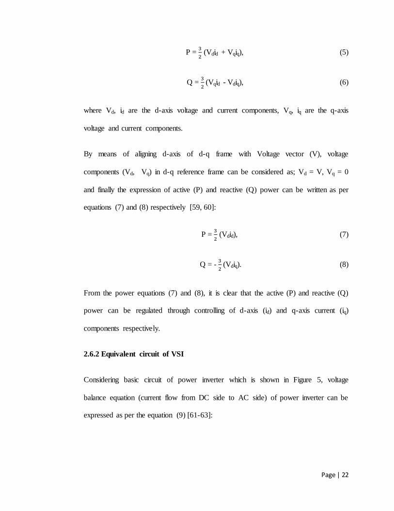
Chapter 2
Page | 22
P =
(Vdid + Vqiq), (5)
Q =
(Vqid - Vdiq), (6)
where Vd, id are the d-axis voltage and current components, Vq, iq are the q-axis
voltage and current components.
By means of aligning d-axis of d-q frame with Voltage vector (V), voltage
components (Vd, Vq) in d-q reference frame can be considered as; Vd = V, Vq = 0
and finally the expression of active (P) and reactive (Q) power can be written as per
equations (7) and (8) respectively [59, 60]:
P =
(Vdid), (7)
Q = -
(Vdiq). (8)
From the power equations (7) and (8), it is clear that the active (P) and reactive (Q)
power can be regulated through controlling of d-axis (id) and q-axis current (iq)
components respectively.
2.6.2 Equivalent circuit of VSI
Considering basic circuit of power inverter which is shown in Figure 5, voltage
balance equation (current flow from DC side to AC side) of power inverter can be
expressed as per the equation (9) [61-63]:

Chapter 2
Page | 23
Figure 5 Basi c system of power inverter [61]
Vabc (out) = Vabc+ Riabc + L
. (9 )
After park transformation (d - q frame), voltage balance equation of power inverter
can be written as per equation (10 ) :
[
] = [
] + R [
] + L
[
] + L [
] [
] (10 )
w here Ud, Uq are the inverter output voltage signal, id (d - axis) and iq (q - axis) are the
inverter output current components, Vd (d - axis) and Vq (q - axis) are the inverter
output voltage components, is the angular frequency (rad/sec), R is the resistance
and L is the inductance betw een inverter output and network .
2.6 .3 Types of VSI control configuration
According to the role of operation, c ontrol configuration of the VSI which is used in
the MG network can be classified into three types namely; grid - feeding, grid -
forming, and grid - supporting power converter. Grid - supporting power converters can
be further classified into grid - support grid - feeding and grid - support grid - forming
type. As per the classification, basic control concept of power inverters is shown in
Figure 6 [64 - 67] . The advantages and disadvantages of each type of VSI is discussed

Chapter 2
Page | 24
below.
Figure 6 (a) Grid-forming; (b) Grid-feeding; (c) Grid-support grid-feeding; (d) Grid-support grid-forming type Inverter [67]
Grid-feeding type inverters are more suitable to operate in parallel with other grid-
feeding type power inverters in grid-connected mode. This type of inverter is
commonly used for DG sources like solar PV and wind turbine in MG network.
Grid-feeding type inverters are not suitable for islanded network of MG, unless there
is any grid-forming or grid-support power inverters are in operation [65-67].
Similarly, the Grid-forming type power inverter is not suitable to operate in parallel
with the utility grid. Poor power sharing and problems of desynchronized phase can
be expected in islanded MG network where the only or more number of grid-forming
type inverters are in operation [66, 67]. GsGfd power converter act as a droop
controlled current source that adjusts the active (P) and reactive (Q) power reference
on the basis of voltage and frequency level measurement in the MG network. Since
the GsGfd power converter is a phase locked loop (PLL) current control driven type,
it needs at least one voltage source power inverter to be online for regulating voltage

Chapter 2
Page | 25
and frequency level in the network, otherwise this type of inverter control is required
to switch over to the grid-forming or GsGfm control when the MG is in transition to
the islanding mode [67]. In addition to fulfill the supply of power to the connected
load, it also ensures regulation of voltage and frequency level in MG network [65,
66].
The GsGfm type VSI acts as a droop controlled voltage source that adjusts voltage
and frequency reference, based on the measurement of active (P) and reactive (Q)
power level in the MG. This type of power inverter behaves as an ideal AC voltage
source which is in series with link impedance (Z). The impedance of the power
inverter is considered as either physical element or virtual impedance, connected
between VSI and MG network.
Previous research works involve the use of grid feeding or grid forming type VSI in
the MG network, the main disadvantage of using the former and latter is that they
can operate only in on-grid and off-grid mode respectively, while it would not be
suitable for on-grid to off-grid transition without the need for additional hardware
for the switching. Hardly research works could be found on the use of GsGfm
type VSI in the MG network as per the author’s knowledge and due to its
ability to operate in both the on-grid and off-grid mode without the need for
rapid mode switching during on-grid to off-grid transition [64-67], GsGfm type
VSI has been utilized for the PV units and battery storage in the on-grid and off-grid
MG model analyzed in this study. The following question will be answered in this
research.

Chapter 2
Page | 26
Whether the GsGfm type VSI ensure smooth operation of the MG
during the on - grid to off - grid transition mode?
2.6 . 3.1 Generic c ontrol configuration of the GsGfm type VSI
Control configuration of Grid - support grid - forming type VSI which is shown in
Figur e 7 mainly includes the following elements; a) power calculation block, b)
droop controller, c) virtual impedance contro l loop, d) voltage control loop and e)
current control loop [64 - 66] .
Figure 7 GsGfm control of power Inverter [66]
In general, droop control concept can be developed on the basis of power flow
conc ept in a typical network. Considering the equivalent circuit of distribution power
network which is shown in Figure 8 , if the power network is in inductive nature
(high X/R ratio) of high voltage (HV) network that the active (P) and Reactive power
(Q) flo w in the network can be can be e x pressed as per the equations (11) and (12 )
respectively [66, 68, 69] :

Chapter 2
Page | 27
Figure 8 Equivalent circuit of distribution power network [69]
P =
Cos -
Cos ( + ) , (11 )
Q =
Sin -
Sin ( + ) , (12 )
w here V1 is inverter output voltage magnitude, V2 is the voltage magnitude of PCC
network, X is the line reactance (inductance), R is the line resistance, is the power
angle, and is the phase angle of line impedance respectively .
Assuming if is (usually) small, hence it is considered that Sin ( ) and Cos ( )
=1 and power flow equations can be expressed as pe r equations (13) and (14 )
respectively:
P =
, (13 )
Q =
. (14 )
As per equ ations (13) and (14 ), real power (P) is in direct relation with power angle
, and reactive power (Q) is in direct relation with voltage difference (V1 - V2)
between DG source and grid network.
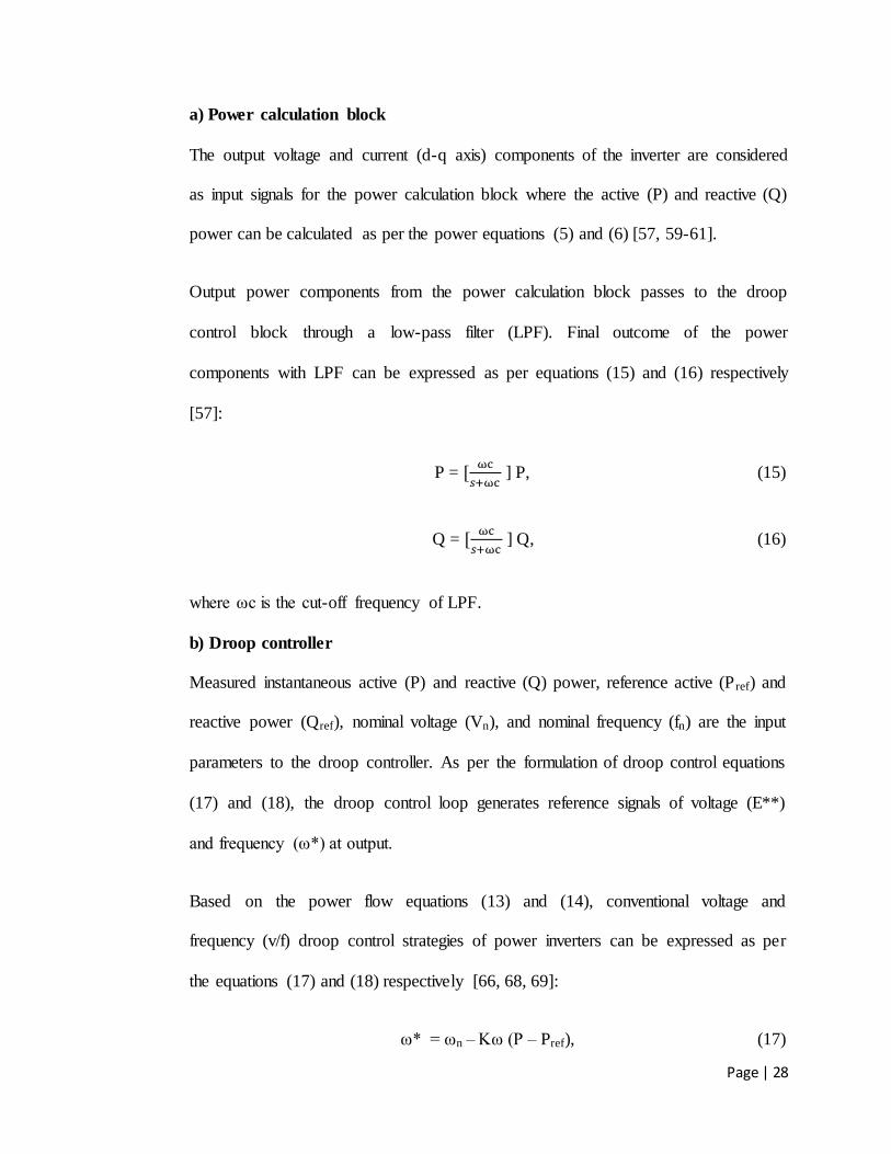
Chapter 2
Page | 28
a) Power calculation block
The output voltage and current (d-q axis) components of the inverter are considered
as input signals for the power calculation block where the active (P) and reactive (Q)
power can be calculated as per the power equations (5) and (6) [57, 59-61].
Output power components from the power calculation block passes to the droop
control block through a low-pass filter (LPF). Final outcome of the power
components with LPF can be expressed as per equations (15) and (16) respectively
[57]:
P =
] P, (15)
Q =
] Q, (16)
where ωc is the cut-off frequency of LPF.
b) Droop controller
Measured instantaneous active (P) and reactive (Q) power, reference active (P ref) and
reactive power (Qref), nominal voltage (Vn), and nominal frequency (fn) are the input
parameters to the droop controller. As per the formulation of droop control equations
(17) and (18), the droop control loop generates reference signals of voltage (E**)
and frequency (ω*) at output.
Based on the power flow equations (13) and (14), conventional voltage and
frequency (v/f) droop control strategies of power inverters can be expressed as per
the equations (17) and (18) respectively [66, 68, 69]:
ω* = ωn – Kω (P – Pref), (17)
Chapter 2
Page | 29
E** = Vn - KV (Q – Qref), (18)
Kω =
(19)
KV =
(20)
where P and Q are the actual active and reactive power, Pref and Qref are the
reference value of active and reactive power, ωn and Vn are the nominal angular
frequency (rad/sec) and nominal voltage level (V), ω* and E** are the reference
angular frequency and voltage magnitude, Kω and KV are the droop coefficients for
active and reactive power, ∆ωmax and ∆Vmax are the maximum deviations of angular
frequency and voltage level, Pmax and Qmax are the maximum real and reactive power
delivered by the power converter.
The voltage reference signal (E**) from the droop controller, passes through the
virtual impedance control loop to the input of the inverter voltage controller. At the
same time, extraction of phase angle (θ) from the frequency reference signal (ω*) of
the droop controller can be used for the application of park transformations in
inverter control system.
c) Virtual impedance control loop
Conventional V/f droop control provides effective power sharing in HV and MV
network where the network is in inductive nature. However in resistive nature of LV
network, conventional droop control is not effective for power sharing among DG
sources due to the coupling effect of active and reactive power. This will result an
inaccurate power sharing among DG sources and affects network stability. In order

Chapter 2
Page | 30
to restrain the circulating current between the DG sources and improve power
sharing through effective decoupling of active and reactive power, a virtual
impedance control can be introduced in inverter control structure [66, 69-71].
Implementation of virtual impedance control loop at output of the power inverter
enhances the decoupling relation between active (P) and reactive (Q) power and
improves power sharing accuracy. Virtual impedance modifies power converter
output voltage reference by subtracting virtual voltage drop from the voltage
reference which is originally generated by the droop controller. Due to the effect of
inverter output current over the virtual impedance, voltage drop across virtual
impedance control loop can be expressed as per the equation (21) [69, 72-74]:
VZD = (E**) – ZD*id, (21)
where VZD is the output voltage drop across virtual impedance, (E**) is voltage
reference from droop control loop, ZD is the virtual impedance, and id is the inverter
output current respectively.
d) Voltage control loop
The Proportional-Integral (PI) based voltage control loop generates a output d-q
reference current (id-ref, iq-ref) signals while comparing modified voltage reference
signal with the actual d-q voltage components (Vd, Vq) at the input side. Expression
of the modified voltage reference signal which is given in equation (22), is a new
voltage reference signal after subtraction of virtual impedance voltage drop from the
original voltage reference signal, generated by the droop controller. By regulating id
and iq current components at the output of inverter, the active (P) and reactive (Q)

Chapter 2
Page | 31
power can be controlled. As per the control configuration of voltage control loop
(Figure 7), the d-q components of reference current (idref, iqref) can be expressed as
per equations (23) and (24) respectively:
Vref (M) = (E** ) - VZD, (22)
Iod-ref = (Vref (M) – Vd)
(23)
Ioq-ref = – (Vq + VZD) (
(24)
where E** is the voltage reference signal, Vref (M) is the modified voltage reference
signal, Vd and Vq are the voltage components in d-axis and q-axis, Id and Id-ref are the
d-axis actual and reference current component, VZD is the voltage drop across virtual
impedance, Iq and Iq-ref are the q-axis voltage actual and reference current component
and Kp and Ki is the proportional and integrator gain of PI controller respectively.
e) Current control loop
The PI based current control loop generates an output voltage signal (Ud, Uq) in d-q
form which is used as reference voltage for PWM block of inverter. In this concept,
in order to improve the performance of PI controller, decouple the d-q components
of voltage and current, and improve the dynamic response of cascade control, the
cross coupling term and the voltage feed forward facility are usually employed [69,
75, 76]. In addition to control of the inverter current, the current control loop is also
responsible to protect the inverter against overload condition. With reference to
voltage balance equation (9), inverter voltage equations in d-q form can be written as
per the equations (25) and (26) respectively [59, 61]:

Chapter 2
Page | 32
Ud = Vd + Rid + L
- ωLiq, (25)
Uq = Vq + Riq + L
+ ωLid. (26)
Thus from the above equations (25) and (26), in order to control id and iq
independently, the coupled term can be decoupled through implementation of current
feed forward compensation technique in the inverter current control loop. As per the
control configuration of current control loop with the inclusion of cross coupling
term and feed forward voltage facility, the inverter output voltage signals of current
control loop can be expressed as per equation (27) [57, 59, 77]:
[
] = [
] [
] + [
] [
] + [
] [
] + [
] (27)
= (id-ref – id);
= (iq-ref – iq),
where Ud and Uq are the output voltage signal in d-q form, ω is the angular frequency
(rad/sec), L is the inductance between the inverter and PCC network, Vd is the d-axis
voltage component, Vq is the q-axis voltage component, Id and Id-ref are the d-axis
actual and reference current component, Iq and Iq-ref are the q-axis actual and
reference current component, Kp and Ki is the proportional and integrator gain of the
PI controller.
Current control loop output reference signals (Ud, Uq) represented in d-q form can be
transformed into a voltage reference signal in the abc-frame (Uabc) through reverse
parks transformation. In order to generate a sine wave form at the appropriate

Chapter 2
Page | 33
reference level, the final voltage reference signal (Uabc) need to pass through the
PWM block. Based on the voltage reference signal (Uabc) and measured phase angle
of the AC network, the PWM block generates pulsing signal for Inverter bridge that
ensures a desired output voltage vector with less harmonics [77-79].
2.7 Power management and Power sharing control
In either (on-grid or off-grid) mode of MG operation, maintaining energy balance is
necessary to get the better regulation of voltage and frequency level in MG network.
In case of any mismatch between the generation and load demand causes deviation in
the voltage and frequency level which creates a negative influence on the quality of
energy supply, thus affecting the performance of sensitive loads connected in the
MG network. In the on-grid mode, regulation of voltage and frequency level in MG
network can be supported by the utility grid. However in off-grid mode, all the DG
sources should be responsible for ensuring power balance and also regulation of
voltage and frequency level in MG network through implemented active coordinated
power management and power sharing control strategies [18, 57, 80].
2.7.1 Co-ordinated power management control – previous research works
Various types of control strategies have been utilized by researchers to ensure better
power management and coordinated operation of DG sources in the PV based MG
network. Y.Wang et al implemented a model predictive algorithm that enables faster
dynamic response in power management during both the on-grid and off-grid mode
of MG operation. In his work, solar PV and battery storage inverters worked in CCM
as grid feeding type during the on-grid mode while battery storage inverter worked in

Chapter 2
Page | 34
VCM (master control) as grid forming type and PV inverter (slave control) in CCM
during the off-grid mode of MG operation [81]. Configuration similar to the Y.Wang
et al was used to maintain the power imbalance in the islanded MG network by Dan
Wu with a control algorithm which follows the bus frequency signal to achieve the
power management in a decentralized manner [45]. Ling showed that power balance
in the MG network can still be achieved during the varying load and solar insolation
conditions through the implementation of co-ordinated control strategies in which
the configuration was different from that of Y.Wang et al and Dan Wu. According to
Ling, battery was operated in the CCM during grid connected mode whereas on the
VCM which follows as per V-f control strategy during the autonomous mode) and
PV inverters were operated in CCM which follows the implementation of dual loop
d-q control algorithm in P-Q control strategy during both mode of the MG operation
[82].
Likewise, Sarina showed that better regulation of the voltage/frequency in the
PV/battery unit based MG network can be achieved through coordinated control
strategies in which PV inverter works on the active/reactive power (P-Q) control and
voltage/frequency (V-f) control method during the on-grid and off-grid mode of MG
operation respectively [83]. Hangtao Shi et al used adaptive virtual impedance and
virtual frequency impedance loop in the inverter control by means of a proposed real
time voltage and frequency compensation strategy (RVFCS) to ensure better
regulation of voltage and frequency level in the PV based MG network [84].
In summary, various types of power management control strategies were developed
and implemented to ensure better power management and coordinated operation of

Chapter 2
Page | 35
DG sources in the PV based MG network. Most of the analysis in PV based MG
network, considered inverter of PV source as grid-feeding type which allows to
operate in P-Q control (CCM) during on-grid and off-grid mode of MG operation,
and battery inverter control was of grid-forming type which allows the inverter to
operate in V-f control (VCM) during islanded mode of the MG operation. The
disadvantages of using the grid-feeding and grid-forming type VSI control in the
MG network have already been discussed in Section 2.6.3.
2.7.2 Power sharing control – previous research works
Conventional P-f and Q-V droop control is more suitable for power sharing among
DG sources in highly inductive nature of distribution network whereas a modified or
reverse P-V and Q-f droop power sharing control is applicable for VSI of the DG
sources in MG power system with resistive nature of LV network [68, 72]. This type
of modified or reverse droop control for MG power system with resistive nature of
LV network is the subject of interest to this study. Several research works on the
modified droop control methods for the DG sources integrated in LV network of the
MG power system have been reported by various researchers and is highlighted
below.
Joseph et al and Xiao et al proposed a novel modified droop controller which uses
resistive output impedance control for the parallel connected single phase inverters
in the islanded MG network. Both were able to achieve improved steady state and
dynamic performance as well as the better power sharing between the DG sources in
the MG network [72, 74]. Ping et al found that dynamic stability of the grid

Chapter 2
Page | 36
connected inverter control can be enhanced during the case of any drift in line
parameters by implementing novel virtual impedance which is composed of virtual
negative resistor (VNR) and virtual inductor integrated into the MG power system
[85]. Previous research works indicate that the use of modified droop controller
in the LV network of the MG power system ensures better power sharing
among DG sources with decoupling of active and reactive power, to improve the
dynamic stability of system in case of any transient conditions, sharing of
harmonic currents in presence of the non-linear load in MG network, etc. In
this research, reverse or modified droop with virtual impedance control
strategy for the VSI of the DG sources (PV and battery) was implemented for
better power sharing in LV network of the developed MG model.
2.8 Need for optimization techniques in the MG network
In a low voltage (LV) MG network, PI-based controllers were commonly used in
VSI of the DG sources. Appropriate selection of the power sharing coefficients and
control parameters of the controller are necessary to improve the control
performance of the system in case of any disturbance or load varying conditions in
the MG network. Through several trial and error methods, appropriate selection of
the control parameters can be done [86]. However, these methods can impose more
complexity and consume more time when dealing with more number of controllers
in the MG power system. In general, due to the lack of inertia and influence of the PI
based inverter controller performance during the transient conditions, power
variation, and variation in voltage and frequency level can be expected more in the
islanded MG network as compared to the grid connected mode. Thus, in order to

Chapter 2
Page | 37
improve the PQ factors in the MG network further in addition to the co-ordinated
power management and power sharing control strategy, optimization techniques can
be implemented in the inverter control system [87]. Overall improvement in reliable
and stable operation of the MG system can be ensured by the application of
optimized control techniques [88, 89].
Modern heuristic techniques with the application of Artificial Intelligence (AI) based
searching algorithms such as; Genetic Algorithm (GA), Particle Swarm
Optimization (PSO), Anti-colony Optimization (ATO), Stochastic diffusion search
(SDS), and Differential Evaluation (DE), etc. can be used for power system
applications to solve the optimization problems in an effective way [80, 90, 91].
GA and PSO algorithms which are based on the computational-intelligence
technique are the most commonly used methods in the MG power system
applications. Since PSO optimization technique is of importance to this study to
improve the PQ factors in the MG network, the basics of the PSO algorithm and its
advantages are discussed below.
2.8.1 Particle Swarm Optimization (PSO) algorithm
The PSO algorithm is a population based stochastic nature of optimization
technique, proposed by Kennedy and Eberhart in 1995 [92-94]. This algorithm
mimics the social behavior of school of fish or flocks of birds or swarm of bees
where they find food in a specific area. Performance of PSO algorithm depends on
the intelligent movement of each particle and collaboration of swarm. Each particle
moves randomly on the basis of its own best knowledge and swarm experience. PSO

Chapter 2
Page | 38
algorithm is useful to determine the objective or fitness function of an optimal
solution in a specific search area. At each iteration, the best position of each particle
(fitness) which is related to the highest fitness value of that particle is called as local
or particle best (Xpbest). Similarly, the best solution acquired by any particle in the
neighborhood of that particle is called as global best (Xgbest) [95].
PSO algorithms can be used for the following control applications such as; optimum
control and regulation of voltage and frequency, optimized power flow and power
control, PQ improvement, optimizing energy and operation management,
minimizing power loss, etc. in the MG network [77, 80, 96].
Optimization performance of PSO does not get affected even when size of the
problem is large and non-linear. As compared to the GA, PSO provides the best
solution due to its following advantages [80, 91].
It restricts the premature convergence problem and offers enhanced search
capability
It is easy to implement and requires less parameters of tuning
It is more flexible and robust than the other conventional techniques, due to
the usage of probabilistic transition rules
It has an effective memory capability than the GA.
2.8.1.1 Basic rules of PSO Algorithm
According to the basic rules of PSO algorithm, main steps of PSO process which is
shown in flow chart of Figure 9, explained in detail as below [93-95, 97]:

Chapter 2
Page | 39
Initialization
It generates (N) number of particles in random and assign initial velocities
randomly for the particles. It then evaluates the fitness value of each particle and
identifies best objective function with best position of particle as the global best.
Finally, it assigns and initializes inertia weight (w) that controls the impact of
previous velocity of the particle on its current velocity
Updating of time
This feature updates the time counter of process
Setting and updating of inertia weight
Setting of dynamic inertia factor (w) can be expressed as per the equation (28).
Inertia weight can be useful to get balance between local and global exploration,
obtain quick convergence with best solution of optimization:
w(t) = – –
– (28)
where t is the current iteration, tmax is the maximum iterations; wmin and wmax
are the minimum and maximum of inertia weight factor
Updating of velocity and position
This option updates the velocity and position of a particle as per the expression
in equation (31) and (32) respectively with reference to the velocity vector (Vi)

Chapter 2
Page | 40
(equation (29)) and position vector (Xi) (equation (30)) in n-dimensional search
space:
Vi = (vi1, vi2, vi3, . . . , vin), (29)
Xi = (xi1, xi2, xi3, . . . , xin), (30)
Vik+1 = wVi
k + c1.r1 [ Xkpbest – Xi
k ] + c2.r2 [ Xkgbest – Xi
k ], (31)
Xik+1 = Xi
k + Vik+1, (32)
where “i” is the index of particle, Vi, and Xi are the velocity and position of
particle “i”, Vik and Xi
k are the velocity and position of particle “i”at iteration
“k”, c1 and c2 are the cognitive coefficients (usually between [0 2]); r1 and r2
are the random numbers (usually between [0 1]) which are generated at each
velocity update, Xkpbest is the local best position of particle “i” which is based on
its own experience, Xkgbest is the global best which is based on overall swarms
experience.
Updating local best (pbest) and global best (Gbest) values
For each particle, it compares current objective value with the objective value of
its Xpbest (particle best) and if current objective value is better, then it updates
Xpbest as the current objective value. Similarly, if its new objective value is better
than objective value of global best Xgbest, then it updates Xgbest with the new

Chapter 2
Page | 41
objective value. Otherwise, it will go again to step of evaluating the objective
function and continue the process.
Stopping criteria
A process can be terminated, if the PSO algorithm completes the maximum
iterations or attains a required level of the fitness value.
Figure 9 PSO process flow chart [95]
2.8.1.2 Cost function
The cost or fitness function determines the behavior of an optimal controller. For the
application of control optimization in the MG power system, four types of time
integral functions namely; Integral Absolute Error (IAE), Integral Square Error
PSO: parameters setting
Initialize population of particles in random with position and velocity
Evaluate Initial fitness of each particle
Set iteration (K=1)
Update velocity and position of each particle
Evaluate fitness of each particle and Update Pbest and Gbest
If K ≤ Max iterationK = K+1
Output optimized results
End
No
Yes

Chapter 2
Page | 42
(ISE), Integral Time Square Error (ITSE), and Integral Time Absolute Error (ITAE)
can be considered. These types are classified under the “minimization of error-
integral function” category [80, 98].
In general, problem of the equality constraints are formulated in objective function
and the constrained optimization problem due to the inequality constraints can be
solved by incorporating constraints into the objective function through the penalty
function method. Penalty function method transforms constrained optimization
problems into the unconstrained optimization problem. If any of the constraints in
response to the system are violated in particular solution, the penalty function
magnifies the weight of the solution (assigning value more than one) to get further
optimization. By incorporating penalty function into the main objective function, the
value of objective function can be increased in case of any condition for constraints
that are violated [92, 99-102].
According to the nature of problem constraints (equality and inequality), the cost
function can be written as per the equation (33):
Cost function (C) = + (33)
The cost function in equation (33) constitutes two terms; first term and second term.
First term f (x) is the fitness function for equality constraints and second term is the
penalty function for inequality constraints. The first term, f (x) can be the
minimization function of control variable (x) and it can be formulated by using any
of the time integral fitness function. The second term is the penalty function that
constitutes penalty factor and violation index of inequality constraint (y).

Chapter 2
Page | 43
2.8.2 Previous research works on the use of PSO optimization in the MG network
Previous studies indicate that the PI controllers in the inverter of the DG sources of
the MG network have been tuned and optimized using PSO algorithms and these
optimized controllers with PSO algorithms show superior performance in
comparison to the conventional PI controllers. Hassan et al formulated a constrained
optimization problem with PSO technique for optimizing non-linear PI controllers of
VSI connected to the MG power system, operated in the autonomous mode [103].
Similarly, Ali Arzani et al applied PSO technique for tuning of PI controllers of the
grid tied PV inverter through an integrated real-time digital simulator (RTDS).
Optimized PI controllers of the PV inverter enhance the dynamic response of PV
system over a wide operating range of solar irradiance condition [104]. PSO
algorithm was also used by En-Chih Chang et al for tuning control gains of Terminal
Sliding Mode Control with fuzzy estimator of Uninterrupted Power Supply (UPS)
inverter leading to enhancement in performance of the UPS inverter with higher
dynamic response during the transient loading conditions [105]. Pablo Garcia-
Trivino et al employed on-line and off-line PSO self-tuning method to tune the PI
controller of the power inverter in hybrid renewable energy system (HRES). Among
the two methods, lowest error indexes and reduction of THD current level was
observed for the online PSO self-tuning as compared to the off-line [106]. Results
from the study of Jordan Radosavljevic indicate that the implementation of PSO
optimization approach solved the both deterministic and probabilistic problems of
Energy and operation management (EOM) under the following operating constraints
such as; stochastic nature of energy from RE sources (PV/wind), uncertainties of

Chapter 2
Page | 44
load condition, varying market price of energy in network with the enhanced overall
efficiency of the MG power system under various operating scenarios [96]. Ma
Yiwei et al proposed a Modified PSO (MPSO) algorithm with cost function
constraints such as; power balance, spinning reserve, output power limit of the DG
units according to their functional role in the islanded MG, start/stop time of DG
units. The proposed PSO algorithm was able to ensure reduction of fuel cost and
emission limit with improvement of the battery life and utilization level of RE
source in the MG network. Apart from tuning of PI controllers in the MG network,
PSO algorithm in the form of Multi- Objective Particle Swarm Optimization
(MOPSO) was used in hybrid power (solar PV/wind) system in which objective
functions were designed to get the best configuration of the system, appropriate
sizing of components along with prediction of lowest loss of power supply
probability (LPSP) and lowest cost of electricity in the network [107].
As per the literature survey conducted by the author, none of the studies could
be found on the use of PSO with proposed cost function for improving the PQ
factors in the MG network implemented with GsGfm type VSI for the DG
units. The following question related to PSO will be answered in this research.
Whether the PQ factors further improve after PSO implementation in
the GsGfm type VSI of the DG units in the MG network during the
transient conditions apart from the implemented power management
and power sharing control?

Chapter 2
Page | 45
2.9 Summary
The literature Section highlighted the concept of solar PV based MG, effect of
various scenarios on the PQ factors, types of VSI, need for co-ordinated power
management and power sharing control and finally, the PSO optimization technique
to improve PQ factors in the MG network. Based on the literature review, the
following research gaps have been identified.
Lack of research on the quantification of PQ factors like VUF, neutral current
variation in voltage/frequency and power variation in the PV based MG
network except THD.
Only individual or a combination of few scenarios has been introduced to
study the PQ issues in the MG network.
Limited experimental works on the PQ analysis in the real-time MG network
implemented with the natural cloud effect and other scenarios
Hardly research works could be found involving the use of GsGfm type VSI
for the DG units in the MG network as per the author‟s knowledge.
No studies on the use of PSO algorithm with proposed cost function to
improve the PQ factors in the MG network implemented with GsGfm type
VSI for the DG units.
Following are the research questions identified based on the literature review
performed:
What is the effect of introducing all the scenarios simultaneously on the PQ
factors in the MG network?

Chapter 2
Page | 46
Does the use of GsGfm type VSI for the DG units in the MG network ensure
smooth operation of the MG during the on-grid to off-grid transition mode?
Whether the PSO algorithm with proposed cost function can further improve
PQ factors in the MG network during the transient conditions apart from the
implemented power management and power sharing control?
This thesis addresses the research gaps and research questions through the
simulation and experimental approach on a PV based MG network.

Chapter 3
Page | 47
CHAPTER 3
Analysis of Power Quality Impacts in a Typical MG Network
3.1 Introduction
In the literature review chapter, it was identified that there was limited studies on the
PQ factors like VUF, variation in power flow and voltage deviation other than the
THD in the PV based MG network. Scenarios like cloud effect, range of PV
penetration levels in the presence of different types of loads, unbalanced load and
unbalanced PV generation has been implemented simultaneously in the MG network
and its influence on the PQ factors has been studied through the PSS SINCAL
software simulation.
The findings from this analysis will help to understand the influence of various
scenarios on the PQ factors of the PV based MG network. The results on VUF,
variation in power and voltage of the PV based MG network which has been
implemented with various scenarios serves as a contribution to the knowledge due to
the lack of intense research with the application of the various scenarios
simultaneously.
Research content of this chapter has been published in the International Conference
on “Sustainable Energy and Environment Engineering” (SEEE2015) and available
online in the Atlantic press publication portal.

Chapter 3
Page | 48
This chapter is organized as follows: Section 3.2 states the detail of MG power
system model development, Section 3.3 describes the method of analysis, Section
3.4 presents the detail of results and discussion, and Section 3.5 concludes the
outcome from this analysis. In appendix A, the features of PSS SINCAL power
system simulation software and the selection of calculation methods which includes
details of calculation settings for balanced Load Flow (LF), unbalance LF, and
Harmonics analysis along with the details of main input data for the proposed MG
model has been provided.
3.2 Development of the MG power system model
A PV based MG was developed using PSS SINCAL and various scenarios have been
introduced and its effect on the PQ factors has been studied in this chapter. Figure 10
shows the schematic diagram of the typical MG power system model developed
using PSS SINCAL. The MG model has been developed based on the energy
demand for a small community along with the provisions for renewable energy to
reduce the environmental impact and inclusion of diesel generator was to ensure
continuous supply of power during non-availability of the main grid supply or
absence of PV generation. The configuration of MV feeders along with the LV loads
was chosen based on the typical residential loads. Different types of loads such as
linear, non-linear and unbalanced loads have been introduced to the model to identify
its impact on the PQ factors. Influence of cloud effect (variation in PV power
generation) on the PQ factors was also studied.
MG model has been configured with four Medium Voltage (MV) feeders (11KV)

Chapter 3
Page | 49
and each feeder has been interconnected to the LV (415V) bus nodes through the
respective Distribution Transformer (11 KV/415V). MV network of the MG model
has been interco nnected with the higher capacity diesel generator (DG) and grid
power source through the step - up transformer (11 KV/66KV). In LV side network,
four bus nodes like: N7, N8, N9, and N10 were configured. Integration of the linear
and non - linear loads at LV bus nodes were organised in the following ways; (1)
linear load at bus nodes N7 and N8, (2) non - linear load at bus node N9, and (3)
composite load (linear + non - linear) at bus node N10. At bus node N8, integration of
single phase loads (unbalanced load ) were considered along with the three phase
linear load. Similarly, integration of single phase solar PV (unbalanced generation)
was considered at bus node N8 and three phase solar PV at other bus nodes N7, N9,
and N10. L1 to L8 are the 11 kV line conductors in which L1 to L4 are in different
lengths and L5 to L8 are in similar lengths, used in MG network.
Figure 10 Schematic diagram of MG power system model

Chapter 3
Page | 50
In this study, the line impedance values for the MV (11KV) feeders in the MG model
have been chosen based on the typical R/X (Resistance/Reactance) ratio of the MV
network which is generally inductive in nature [66]. Also in this model, the installed
capacity of PV generation (100%) which is equivalent to the capacity of total load
connected at each LV bus node has been considered. The sizing of DG installed
capacity (3250 KVA) has been chosen such that it could meet the 95% of total
capacity of load (3410 KVA) in the MG network. This configuration was chosen so
as to improve the reliable operation of MG during non-availability of power
generation from solar PV as well reduce the dependency of power support from the
main grid source. The specification of the network elements like; power sources,
Transformers, line conductors, and Loads are given in the Tables (1) to (5)
respectively and these specifications were selected based on the typical load
demands in the residential areas. The specifications are chosen such as to ensure
reliable and balanced generation (balancing the generation and demand) in the MG
network.
Table 1 Specification of Grid source and Diesel generator
Grid Source Rating
Short circuit power 100 MVA
Network voltage level 66 KV
Diesel Generator Rating
Rated Apparent Power 3.25 MVA
Generator Voltage 2.4 KV
Operating power factor 0.9

Chapter 3
Page | 51
Table 2 Specification of DG sources
Power Sources Capacity Bus Node Voltage
Three phase Solar PV 1 1000 KW N7 0.415 KV
Single phase Solar PV 2a/2b/2c 10 KW/100 KW/200 KW N8 0.240 KV
Three phase Solar PV 3 500 KW N9 0.415 KV
Three phase Solar PV 4 1000 KW N10 0.415 KV
Diesel Generator (DG) 3250 KVA N2 2.4 KV/11 KV
Table 3 Specification of Transformers
Main Transformer (MTX) Distribution Transformer (DTX)
Rated Apparent Power 8000 KVA Rated Apparent Power 1000 KVA
Rated Voltage (primary) 66 KV Rated Voltage (primary) 11 KV
Rated Voltage (secondary) 11 KV Rated Voltage (secondary) 0.415 KV
Short circuit voltage 8 % Short circuit voltage 4 %
Table 4 Specification of loads
Type of Loads Capacity Bus nodes
Linear (LO1) 1000 KVA N7
Linear (LO2) 500 KVA N8
Single phase Linear (LO2a/LO2b/LO2c) 300 KVA/100 KVA/10 KVA N8
Non-Linear (LO3) 500 KVA N9
Linear + Non-Linear (LO4a +LO4b) 500 KVA + 500 KVA N 10
Table 5 Specification of line conductor (11 KV)
LINE L1 L2 L3 L4 L5 L6 L7 L8
Length (KM) 0.41 0.34 0.36 0.40 0.16 0.16 0.16 0.16
Parameters/KM R = 0.28 Ω; X = 0.36 Ω; C = 10.5 Nano Farad

Chapter 3
Page | 52
3.3 Method of Analysis
PQ impacts like; power variation, voltage variation, unbalance voltage level, current
and voltage harmonic distortions were analysed in the developed MG network
model, using PSS SINCAL. Power variation and voltage variation level in MG
network were analysed through the symmetrical load flow analysis. Similarly,
current and voltage THD level were analysed at the LV bus nodes of MG network
through harmonic analysis. In addition, unbalance voltage levels in LV network was
estimated through the unbalanced load flow analysis.
3.3.1 Load flow analysis
In this analysis, Newton-Raphson method of load flow analysis was considered
according to typical daily load and solar profile condition. The amount of solar
radiation that reaches a solar panel is not only based on the sun position in the sky,
also depends on the amount of clouds passing between the sun and solar panel [27].
Solar disturbance due to the cloud effect can be considered as one of the main reason
for power intermittency in the PV output. PV power intermittency can be considered
in different time scales like; “second” level causes voltage flicker and “minute” level
affects the regulation of power generation reserve in power system [108]. During this
analysis, a typical cloud pattern varying in minute‟s level as shown in Figure 11 was
considered to quantify the effect of power variation in generation side and voltage
variation level at the LV bus nodes of MG network.

Chapter 3
Page | 53
Figure 11 Typical daily solar profile with solar disturbance
3.3.1.1 Power and voltage variation
PV power variation due to the cloud effect reflects the corresponding power flow
variation from generation side during on-grid and off-grid mode of MG operation.
During the on-grid mode of MG operation, where the grid source is considered as
main power source, significant power variation from the PV output creates a
situation for an urgent need of power generation reserve and regulation from the grid
source. Similarly, when the diesel generator unit is considered as main power source
during the off-grid mode of MG operation, output power variation of solar PV
creates a situation for the frequent ramp up and ramp down of power requirement
from the diesel generator, which will lead to increase in wear and tear effect of
conventional power unit components, increase in maintenance cost, and thereby
reducing the efficiency of diesel generator.
In LV network, Voltage fluctuation can be caused by the effect of frequent power
variation from the PV output. Due to the cloud effect, frequent active power
variation from the PV output can cause significant voltage variation, particularly in
004:00
0.2
0.4
0.6
0.8
08:00 20:0016:0012:00 24:0000:0
Time (hour)
Solar disturbance
Sola
r In
sola
tion
(p.u
)

Chapter 3
Page | 54
the LV network. This is due to the weak LV feeders which are located far away from
the main substation, having lower fault level, and high R/X ratio [109]. The rapid
voltage variation can cause a negative influence over the quality of energy supply to
the loads, affects the functional operation of protective devices, and voltage
regulators in upstream network, etc. As per AS 60038 standard [110, 111], the
tolerance level for voltage variation in LV network should be around +10% and -6%
with reference to its nominal voltage level (single phase: 230V and three phase:
400V).
3.3.2 THD analysis
Harmonics are the frequencies that are integer multiples of the fundamental
frequency. Power Electronics (PE) converter and non-linear loads are the main
causes for current harmonics domination in the MG network. Due to the system
impedance, harmonic current injected into the supply system can cause the rise of
voltage harmonics. During this analysis, harmonics level were estimated on the basis
of solar PV penetration level with respect to the type of load (linear and non-linear)
which are connected in LV network of the MG power system.
3.3.2.1 Total Harmonic Distortion (THD)
THD is the ratio of sum of r.m.s (root mean square) value of all the harmonic
components up to a specific order to the r.m.s value of fundamental component.The
expression for current and voltage THD can be written as per the equation (34) and
equation (35) [112] respectively:

Chapter 3
Page | 55
THDI √
(34)
THDV √
(35)
where Ih1 is the fundamental current harmonic, Uh1 is the fundamental voltage
harmonic, Ihn is the current harmonic at highest order and Uhn is the voltage
harmonic at highest order.
The current and voltage THD were estimated in the MG network at different PV
penetration levels with respect to the load, connected in each LV bus node in the
following manner; at different PV penetration levels with respect to the linear load
(100% linear), non-linear load (100% non-linear), and composite load (50% linear +
50% non-linear). In PSS SINCAL, the voltage and current THD level can be
estimated on the basis of network impedance between a defined starting and ending
frequency at given frequency step with additional consideration of current harmonics
data (refer Appendix Section ) for PV inverters and non-linear loads. However, no
harmonic filters in the MG network were included during this harmonics analysis.
Due to the effect of higher level PV penetration and presence of non-linear loads, the
domination of current harmonics can be expected in the MG network. Excessive
harmonics can cause the following issues; overheating of transformers and cables,
increase system power loss, affects the accuracy of measuring instruments, creates
malfunction of protective relays, increases thermal stress in capacitor bank etc. in the
power system network [19, 113]. According to AS 4777 standard [110], maximum

Chapter 3
Page | 56
limit of current harmonics (up to 50th order) injection from the grid connected PV
inverter should be less than 5 %. Similarly, as per AS / NZS 61000.2.2 [111],
compatibility level of voltage THD in the LV distribution network should be less
than 8%.
3.3.3 Unbalance voltage analysis
Voltage unbalance is a significant PQ issue in the distribution network of the MG
power system. Unbalance current is a root cause for the unbalance voltage in the
network. Unbalancing in network may occur due to several factors such as; the
uneven distribution of single phase load, single phase DG units in network, unequal
impedance of three phase distribution network, and unbalanced three phase loads in
network, etc. [114]. In PSS SINCAL, unbalance voltage level was estimated through
the unbalanced load flow analysis. For this analysis, typical uneven distribution of
single phase loads and uneven distribution of single phase PV units were considered
in LV bus node of the MG network.
3.3.3.1 Unbalance voltage
The unbalance voltage level which is defined in unbalance voltage factor (VUF) is
expressed in percentage (%). Generally, VUF can be calculated by two methods
such as; National Electrical and Manufacturers Association (NEMA), and
International Electro technical Commission (IEC). NEMA definition of VUF is
expressed in equation (36) and IEC definition of VUF is expressed in equation (37)
respectively [114, 115]:

Chapter 3
Page | 57
VUF
(36)
(%), (37)
where Vn and Vp are the negative and positive sequence voltage, Vab , Vbc, and Vca, are
the line voltages, and Vmean is average values of Vab, Vbc,Vca,.
Excessive unbalance voltage level due the effect of unbalancing in the MG network
can have a significant impact on de-rating of the induction motor causing increased
heating and losses, increased thermal stress for variable speed drive (VSD)
electronic components with the addition of triplen harmonic current, mal-operation
of protective system, affects the performance of power metering devices, excessive
neutral current, etc. [19, 114].
As per the AS/NZS 61000.2.2 standard, maximum allowable level of unbalance
voltage in the LV network should be around 3% [111].
3.4 Results and Discussion
In this Section, overall simulation results given in the Table 6 (for power variation
and voltage variation) and Table 7 (for THD and unbalance voltage level) are
discussed in detail.
Table 6 Results of power variation and voltage variation
Effect of Solar disturbance Simulation Results – 1
During solar disturbance (11:00 to 11:40 hours)
Power variation Minimum 800 KW to Maximum 1520 KW
Voltage variation 95.8 % to 96.8 % at LV bus node N7

Chapter 3
Page | 58
Table 7 Results of THD and Unbalance voltage level
Standard LimitSimulation Results – 2
Node N7 Node N9 Node N10 PV Penetration
Current THD < 5 %
> limit > limit > limit 100 %
> li mit > limit > limit 70 %
< limit > limit > limit 50 % - 30 %
Voltage THD 8 %
> limit > limit > limit 100 %
< limit < limit < limit 70 %
< limit < limit < limit 50 % – 30 %
Unbalance Voltage < 3 % Unbalance voltage level around 1.48 % at Node N8
3.4 .1 Power variation - Results discussion
A typical cloud effect of solar disturbance was introduced in the daily solar profile
for each PV (100 KW ) with total installed capacity of around 1 MW, connected at
the LV (415 V) bus node N7. As shown in Figure 12 , during this period of solar
disturbance (from 11 hours to 11:40 hours), the power variation from each PV output
was observed from minimum 0 KW to maximum 73 KW .
Figure 12 PV power variation during solar disturbance

Chapter 3
Page | 59
Figure 13 Power flow from generation side (Grid/DG unit)
Active and reactive power flow from supply sources (Grid source/diesel generator
unit) according to the daily load profile is shown in Figure 13. Due to this
cumulative effect of power variation from all the ten PV units, corresponding power
flow variation from generation side was observed. During on-grid mode of the MG
operation, the power flow variation observed from the grid side was minimum 800
KW to maximum 1520 KW. Also same level of power variation was observed in the
diesel generator unit during off-grid mode of the MG operation. Figure 14 shows the
maximum and minimum power flow variation, observed during the time of solar
disturbance from the grid side and in diesel generator
Figure 14 Power variation during solar disturbance (Grid/Diesel generator)
0
400
800
1200
1600
2000
2400
2800
00:00 04:00 08:00 24:0012:00 16:00 20:00
Time (hours)
kW
Power variation
800 kW
1520 kW
800
1000
1200
11:10
1400
1600
11:20 11:30 11:40

Chapter 3
Page | 60
Thus the cloud effect causing the power variation from solar PV, created a situation
for urgent need of power reserve and power regulation from grid side during on-grid
mode of the MG operation. Similarly, in off-grid mode, the power variation from PV
units was compensated through the frequent ramp up and ramp down operation of
diesel generator.
3.4.2 Voltage variation-Results discussion
During PV power variation (from 11:00 to 11:40 hours), a variation in voltage level
(Figure 15) was observed at LV bus node N7 where the solar disturbance was
introduced for the connected PV units. As shown in Figure 16, the maximum and
minimum level of voltage was observed around 96.8% and 95.8% respectively at LV
bus node N7.
During the solar disturbance, variation in voltage level at LV bus node N7 was
observed to be minimum (1% only) and well within the limit as per AS 600038
standard. However, in case of large level of PV integration in a weak network or at
peak load with low voltage condition, this voltage variation may reach a significant
level. Also, frequent and more number of variations in the voltage level can create a
negative influence over the quality of energy supply. This kind of voltage variation
in the PV based power network due to PV power variation caused by cloud effect
was also reported by Cheiw Yun Lau et al and Achim Woyte et al [42, 43].

Chapter 3
Page | 61
Figure 15 Voltage level of all three phases
Figure 16 Voltage variation (during solar disturbance)
3.4.3 Current and voltage THD-Results discussion
Voltage and current THD in the MG network were analysed for a range of
percentage of PV penetration levels in reference to the connected total linear load at
LV bus node N7, non-linear load at LV bus node N9, and composite load (linear +
non-linear) at LV bus node N10 respectively. The level of THD is based on the
percentage of PV penetration level (with respect to the connected load) and type of
load (linear, non-linear, and linear + non-linear) connected in the network. In
96
97
98
00:00 04:00 08:00 12:00 16:00 20:00
V(%
)
Time (hours)
Voltage variation
95.8 %96
11:10 11:20 11:30 11:4011:00
97
96.5
96.8 %

Chapter 3
Page | 62
general, THD results were observed for 30%, 50%, 70% and 100% PV penetration
level and acce ptable PV penetration level was identified in each node which is
co rresponding to the THD level as per the standard limit . If the THD results exceed
the standard limit below the 30% PV penetration level for any node (based on the
nature of load) , it will also be highlighted. These PV penetration levels have been
chosen in wide range to find the acceptable level in which the THD corresponds to
the standard limit in each node. Integration of PV with the different types of load
arrangement, considered for the harmonics analysis is shown in Figure 17 .
Fi gure 17 Integration of PV with different types of loads at LV bus nodes
Figure 18 harmonics current curve of typical PV inverter
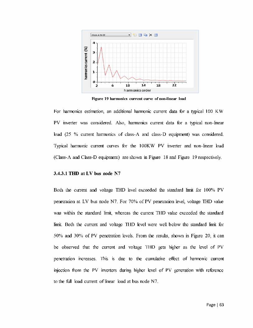
Chapter 3
Page | 63
Figure 19 harmonics current curve o f non - linear load
For harmonics estimation, an additional harmonic current data for a typical 100 KW
PV inverter was considered. Also, harmonics current data for a typical non - linear
load (25 % current harmonics of class - A and class - D equipment) was consid ered.
Typical harmonic current curves for the 100KW PV inverter and non - linear load
(Class - A and Class - D equipment) are shown in Figure 18 and Figure 19 respectively.
3.4 .3.1 THD at LV bus node N7
Both the current and voltage THD level exceed ed the standard limit for 100% PV
penetration at LV bus node N7. For 70% of PV penetration level, voltage THD value
was within the standard limit, whereas the current THD value exceeded the standard
limit. Both the current and voltage THD level were well b elow the standard limit for
50% and 30% of PV penetration levels. From the results, shown in Figure 20 , it can
be observed that the current and voltage THD gets higher as the level of PV
penetration increases. This is due to the cumulative effect of harmon ic current
injection from the PV inverters during higher level of PV generation with reference
to the full load current of linear load at bus node N7.

Chapter 3
Page | 64
Figure 20 PV with linear load at LV bus node N7
3.4 .3.2 THD at LV bus node N9
As per the THD results at bus node N9 shown in Figure 21 , current THD values for
all the PV penetration levels were significantly high as compared to the bus node N7
and also found to be above the standard limit. In case of 100% PV penetration level,
volt age THD was observed to be just above the standard limit (8.1 %) whereas it was
within the standard limit for all the other penetration levels. This is only due to the
effect of non - linear load (class - A and class - D equipment) connected at bus node N 9.
In c ase of the LV bus node N9, current THD at 10% PV penetration level was
presented, since the current THD level appears to exceed the standard limit at that
minimum penetration level due to the effect of non - linear load connected to N9 .

Chapter 3
Page | 65
Figure 21 PV with non - linear load at LV bus node N9
3.4 .3.3 THD at LV bus node N10
THD results at bus node N10 shown in Figure 22 , it is to be noted that the current
THD values were high and above the standard limit for all considered PV pene tration
levels (30%, 50%, 70% and 100%) and in this case, the current THD values were
within the standard limit only for the PV penetration level of 20% . Voltage THD
values were found to be below the standard limit for all the penetration levels
except100% . Voltage and current THD values at bus node N10 were low as
compared to their counterparts at bus node N9. This is due to the effect of composite
load where the linear and non - linear loads are distributed in equal (50%) proportion
at bus node N10.

Chapter 3
Page | 66
Figu re 22 PV with composite load at LV bus node N10
Results from the Figure 20 , Figure 21 , and Figure 22 , clearly indicates that the THD
reaches a significant level in case of higher level of PV penetrations, and amount of
non - linear l oad present in the MG network. This is in agreement with the results of
previous researchers work who indicated that THD level in the MG network depends
highly on the PV penetration level and the type of load connected to the network
[37] . The high level of THD can cause power losses, overheating of conductors,
transformers, capacitor banks, motors or generators, and exc essive current in neutral
line etc.in the MG network.
3.4 .4 Unbalance Voltage - Results discussion
The u nbalance voltage level was estimated at the LV bus node N8 while considering
uneven distribution of single phase PV units and single phase loads in the LV
network. At LV bus node N8, shown in Figure 23 , the single phase solar PV units
and single phase loads were distributed in each phase as follows; 10 KW solar PV
and 300 KVA load in phase - A, 100 KW PV and 100 KVA load in phase - B, 200 KW
PV and 10 KVA load in phase - C respectively.

Chapter 3
Page | 67
Figure 23 Uneven distribution of the loads and PV units
The voltage profile of each phase in LV bus node N8 according to the typical daily
load profile is shown in Figure 24.
Figure 24 Unbalance voltage profile at LV bus node N8
As per the daily load profile, it was observed that during peak load period (12:30
hrs), the voltage level difference between phase-A and phase-C was more compared
to that of low demand period (05:30 hrs). The voltage level in phase-A was low
around 96.2% (399 V), whereas in phase-C was around 99.4 % (413 V).
0:00 12:00 16:004:00 8:00 20:00 24:00
95.0
98.0
99.0
96.0
97.0
Time (hours)
V (
%)
PEAK LOAD
LOW DEMAND

Chapter 3
Page | 68
Figure 25 Unbalance voltage level at LV bus node N8
Through this analysis, the unbalance voltage level at bus node N8 was estimated and
found to be within the standard (AS/NZS 61000.2.2) limit of around 1.48% (Figure
25). However, this value may vary according to the load condition as per the voltage
profile shown in Figure 24 and also it can increase further above the standard limit in
case of any large LV distribution network with the uneven impedance level, uneven
distribution of single phase loads and PV generation in LV network. The change in
magnitude of the unbalance voltage level in the power system network due to the
unbalanced load and unbalanced generation was also reported by Trichakis et al and
Nagarajan [40, 41]. The excessive unbalance voltage in the LV network can have a
significant impact on de-rating of the induction motor with increased heating and
losses, increased thermal stress for variable speed drive (VSD) electronic
components, etc.
3.5 Conclusion
PQ issues like; power variation, voltage variation, THD, and unbalance voltage level
were analysed and quantified in a typical PV based MG model through the
simulation in PSS SINCAL software at various scenarios. These PQ factors were

Chapter 3
Page | 69
compared to its respective standard limit. As mentioned before, in the developed
model, various scenarios have been simultaneously introduced like cloud effect in
presence of the linear load for the PV units, non-linear and composite loads,
unbalanced load and unbalanced PV generation in the bus nodes of the MG network.
Based on the simulation results, it was found that
Voltage and current THD showed an increasing trend at higher PV
penetration levels in all the bus nodes of the MG network similar to the
results obtained by the previous researchers.
Introduction of the non-linear and composite loads in the presence of
different PV penetration levels have significant influence on the current THD
in the node to which the load is connected. This has not been reported
previously in the literature as per the author‟s knowledge.
Power variation from the solar PV output due to solar disturbance (cloud
effect) caused corresponding effect of power flow variation in both the grid
source and diesel generator unit during the on-grid as well as off-grid mode
of the MG operation. PV output power variation also caused local voltage
variation at the LV bus node, where the solar disturbance was introduced for
the connected PV units.
VUF was influenced by the uneven distribution of the single phase PV units
and single phase loads. However, the value was below the standard limit.
VUF was found to be significantly high during the peak demand period as per
the daily load profile. This is a new finding as the previous studies have not
reported it.

Chapter 3
Page | 70
To conclude, the influence of each scenario implemented simultaneously could be
seen in the PQ factors of the PV based MG network. This research differs from the
previous work due to the introduction of various scenarios simultaneously in the MG
network.

Page | 71
Chapter 4
Experimental analysis of Power Quality in a real MG network
4.1 Introduction
In the previous chapter, multiple scenarios were introduced in the PV based MG
network to study its impact on the PQ factors through simulation. This chapter
addresses one of the research gaps highlighted in this thesis (Section 2.4) which is
the limited amount of experimental works on PQ analysis of the real-time PV based
MG network implemented with the real cloud effect and other scenarios.
The main PQ issues like; Voltage and frequency variation, unbalance voltage, neutral
current level and THD were analyzed in a real-time MG network through the
experiments in the CSIRO REIF facility in Australia. THD analysis was carried out
at different PV power levels (with respect to the maximum PV power rating) during
the real cloud effect in the MG network. Apart from the overall THD results, the
individual odd order harmonics in the MG network have also been reported. The
variation in voltage and frequency level in the MG network was also analyzed by
introducing various transient conditions (sudden load and generation changes) in
presence of the real cloud effect during the on-grid and off-grid mode of MG
operation. This make the work unique compared to the previous works in the
literature.

Page | 72
Content of this chapter has been published in the “Journal of Power and Energy
Engineering” (Volume 4; Number 4 (April 2016); pp. 17-34), Scientific Research
Publishing Inc.
This chapter is organized as follows: Section 4.2 presents the configuration of MG
network and details of MG associated elements, at CSIRO REIF, Newcastle-
Australia. Section 4.3 describes the details of PQ issues and its effect on the MG
network and also describes the standard limit for PQ level. Section 4.4 defines the
method of analysis, 4.5 addresses the results in detail, and Section 4.6 concludes the
outcome from this study.
4.2 MG Network configuration
MG in CSIRO facility has been configured with new grid management technologies
and efficient energy mix from the various types of Micro power sources and
controllable load bank in a low voltage (LV) power system network. An efficient
control of DG sources and high speed data acquisition can be done through
Supervisory Control and Data Acquisition (SCADA) system facility available from
the central control room. The Data Acquisition (DAQ) system has the facility to
collect and logging the power system network data at higher sampling rate (50,000
samples/second) effectively. The MG network is interconnected with Utility grid
through a single Point of Common Coupling (PCC) and the MG is capable of
operating in both “on-grid” and “off-grid” mode of operation. A single line diagram
of MG network configuration at CSIRO REIF is shown in Figure 26. The
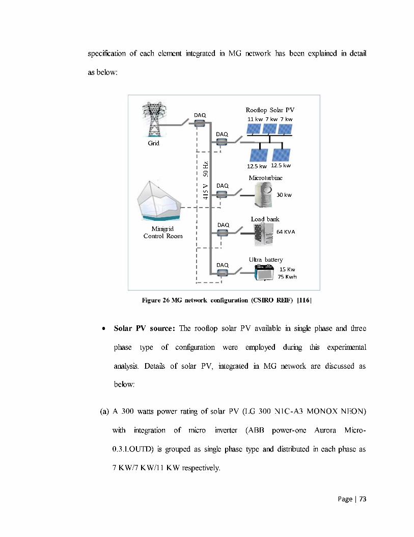
Page | 73
specification of each element integrated in MG netwo rk has been explained in detail
as below:
Figure 26 MG network configuration (CSIRO REIF) [116]
Solar PV source : The r ooftop solar PV available in single phase and thre e
phase type of configuration were employed during this experimental
analysis. Details of solar PV, integrated in MG network are discussed as
below:
(a) A 300 watts power rating of solar PV (LG 300 N1 C - A3 MONOX NEON)
with integration of micro inverter (A BB power - one Aurora Micro -
0.3.I.OUTD) is grouped as single phase type and distributed in each phase as
7 KW/7 KW/11 KW respectively.
Page | 74
(b) In addition, two numbers of solar PV (Mono crystalline Silicon cell) with
each power rating of around 12.5 KW were integrated with 15 kVA three
phase inverter (SMA Sunny (15,000 TL) Tripower Economic Excellence).
Micro Turbine (MT) Generator: Micro Turbine (Capstone C30) used in the
real MG network is a gas operated, compact and ultra-low emission
generator operating with maximum power rating of around 30 KW. MT
coupled synchronous generator supplies power to the MG through a back to
back (AC-DC-AC) converter. MT acts as a master power source to fulfill the
energy requirement in MG network during the “Off-grid” mode of MG
operation.
Battery Storage : Operating voltage and Ampere hour capacity of each Ultra
battery (Make: Furukawa) storage unit was around 24V and 1000 Ah
respectively. Three units of battery storage that were available in the
laboratory and each storage unit (5 KW/24 KWh) were integrated with the 5
kVA AC inverter (Selectronic PS1-single phase) in each phase. The
operation of battery storage can be done through the manual control.
Load Bank: A 64 kVA rated capacity load bank is available with the
configuration of RLC (Resistor (R), Inductor (L), and Capacitor (C))
elements. The load bank can be operated as per the programmed typical load
profile and also it can be operated through a manual command.
Data Acquisition (DAQ): Each source of elements in MG has its own DAQ,
which collects the measured power parameters at higher speed rate. The
DAQ for grid side (PCC point), solar PV, Micro Turbine, and Load bank are

Page | 75
named as follows: DB DAQ, PV DAQ, MT DAQ, and Load DAQ
respectively.
4.3 Description of PQ Issues
The term PQ in electrical network refers to maintaining wave form of voltage and
current close to pure sinusoidal at the rated magnitude and frequency [114]. Main PQ
issues like; voltage and frequency variations, current and voltage harmonic
distortions, unbalance voltage and current level in neutral line of MG network were
analyzed in this study.
4.3.1 Frequency and Voltage Variation
In order to get better voltage and frequency regulation in the MG network, it is
necessary to maintain energy balance (Generation = Consumption) every time [19].
However, due to the power variation from intermittent nature of RE sources and
varying active and reactive power demand in the distribution network, always there
is a chance of voltage and frequency variation in the power network. In the “on-grid”
mode of MG operation, grid acts as a buffer to maintain energy balance easily,
whereas in the “Off-grid” mode, maintaining voltage and frequency variation within
the tolerance level through energy balance is a major task in the MG network. This is
due to the lack of power inertia availability, challenges associated with the
coordinated operation, and control of different types and characteristics of DG
sources. Excessive variation of voltage and frequency can create a negative influence
on the quality of energy supply and affects the performance of sensitive load
connected in MG the network.

Page | 76
Allowable operating range of frequency and Voltage (standards)
Nominal operating frequency of the power network is around 50 Hz in
Australia. In National Electricity Market (NEM) regions, network frequency
is maintained by Australian Energy Market Operator (AEMO). Allowable
operating range of frequency level as per the Australian Network standard
(NEM) is given in Table 8 [110, 117]. As per the AS 60038 standard [110,
111], allowable operating range of voltage level in LV network is given
Table 9.
Table 8 Acceptable range of frequency level as per Network standard (NEM) [110]
Frequency Standard Conditions
Containment (99 % of the time)
Stabilization/Recovery (within 5 minutes)
No contingency event 49.85 Hz to 50.15 Hz 49.85 Hz to 50.15 Hz
Generation event or load event 49.5 Hz to 50.5 Hz 49.85 Hz to 50.15 Hz
Table 9 Acceptable range of voltage level as per AS 60038 standard [110]
Nominal Voltage level Allowable voltage level
Max (V) Min (V)
230 V (phase to neutral) 253 V (+ 10 %) 216 V (- 6 %)
400 V (phase to phase) 440 V (+ 10%) 376 V (- 6%)
4.3.2 Unbalance Voltage and Neutral Current
Definition of unbalance voltage and unbalance current, impacts of the unbalance
voltage in power system network, and IEC, NEMA methods of calculation for
unbalance voltage level are already explained in Section 3.3.3.1 of Chapter 3.
Excessive neutral current level due to the effect of unbalance, leads to overloading of
the distribution feeder and transformer with the addition of creating heat losses.

Page | 77
Also, the neutral current caused common mode voltage affects the performance of
sensitive electronic equipment‟s connected in the network [19, 114].
The neutral current (IN) can be calculated as per the equation (38) [118]:
√
(38)
where IA, IB, IC are the phase RMS current values.
Allowable unbalance voltage level
As per the Australian standard AS/NZS 61000.2.2 [111], maximum
allowable unbalance voltage level for the LV network should be around 3%.
In LV network, the allowable unbalance voltage level over the average period
of 1 minute, 10 minutes, and 30 minutes is shown in Table 10.
Table 10 Compatibility of unbalance voltage level in LV network [111]
Unbalance Voltage Negative sequence voltage (% of nominal voltage)
No contingency event
Credible contingency event
General Once per hour
Average period (minutes) 30 30 10 1
LV Network ( < 10 KV) 2 % 2 % 2.5 % 3 %
4.3.3 Total Harmonic Distortion (THD)
Definition and negative impacts of THD in power system network, method of
calculating current and voltage THD level are explained in detail in the Section
3.3.2.1 of Chapter 3.
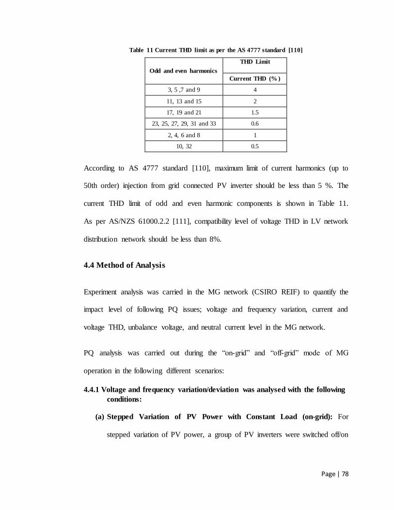
Page | 78
Table 11 Current THD limit as per the AS 4777 standard [110]
Odd and even harmonics
THD Limit
Current THD (% )
3, 5 ,7 and 9 4
11, 13 and 15 2
17, 19 and 21 1.5
23, 25, 27, 29, 31 and 33 0.6
2, 4, 6 and 8 1
10, 32 0.5
According to AS 4777 standard [110], maximum limit of current harmonics (up to
50th order) injection from grid connected PV inverter should be less than 5 %. The
current THD limit of odd and even harmonic components is shown in Table 11.
As per AS/NZS 61000.2.2 [111], compatibility level of voltage THD in LV network
distribution network should be less than 8%.
4.4 Method of Analysis
Experiment analysis was carried in the MG network (CSIRO REIF) to quantify the
impact level of following PQ issues; voltage and frequency variation, current and
voltage THD, unbalance voltage, and neutral current level in the MG network.
PQ analysis was carried out during the “on-grid” and “off-grid” mode of MG
operation in the following different scenarios:
4.4.1 Voltage and frequency variation/deviation was analysed with the following conditions:
(a) Stepped Variation of PV Power with Constant Load (on-grid): For
stepped variation of PV power, a group of PV inverters were switched off/on

Page | 79
in stepped level along with integration of constant load was considered
throughout the analysis.
(b) Frequent power variation and load variation (on-grid): A frequent
variation in power generation which is equivalent to a minute‟s level
variation of solar irradiance in a typical solar profile along with variation of
load was considered.
(c) Actual PV Power Variation with the constant Load (off-grid): Actual PV
power variation due to a real solar disturbance of roof top PV was
considered along with integration of constant load in the islanded MG
network
The observed variation in frequency level from both the on-grid and off-grid analysis
was compared with the acceptable operating range of frequency level as per the
Australian Network standard (NEM) [110, 117] and similarly voltage level was
compared with the acceptable operating range of voltage level as per the AS 60038
standard [110, 111]. Since the nominal voltage and frequency level of IEEE 1547 is
different from the nominal voltage and frequency level of Australian network and
there is no standard specification officially for MG in Australia. Therefore, in this
study, observed frequency and voltage level in the MG network during the analysis
has been compared with the acceptable operating range of frequency and voltage
level as per the Australian network standard (NEM) and AS 60038 standard
respectively.

Page | 80
4.4.2 Unbalance Voltage and Neutral Current analysis
Uneven distribution of single phase PV generation and single phase load in the MG
network was considered during this analysis. The calculated unbalance voltage factor
(VUF) from the experiments was compared with AS/NZS 61000.2.2 standard.
4.4.3 THD analysis
Various power levels of PV output (P0) with respect to their full power rating (Pr) of
overall PV installed capacity in each phase line of MG network were considered.
The odd and even harmonic current components were analysed and calculated, then
the current and voltage THD results were compared with AS 4777 and AS/NZS
61000.2.2 standard level respectively.
Current and voltage THD level was quantified in each phase line at various power
levels of PV output (P0) with respect to their full power rating (Pr) of overall PV
installed capacity. Variation in actual solar irradiance which creates the
corresponding variation in PV power generation over the certain period of time was
considered for this analysis.
4.5 Results and Discussion
In this Section, various results (Voltage/frequency variation, unbalance
voltage/neutral current, and voltage/current THD) obtained from the MG network
analysis are discussed in detail.

Page | 81
4.5.1 Results of Voltage and frequency variation/deviation
Voltage and frequency variations/deviations were estimated in the MG network
during on-grid and off-grid mode of the MG operation at the following conditions;
stepped variation of PV power with constant load (on-grid), actual PV power
variation with constant load (off-grid), and frequent power variation and load
variation (on-grid).
4.5.1.1 Stepped Variation of PV Power with Constant Load: On-Grid Mode
Nominal operating voltage in LV network of the MG at CSIRO REIF is considered
around 415 V. Installed capacity of PV with 50 KW power rating was integrated
along with 64 kVA power rating of load bank in LV network of MG power system.
Figure 27 shows the MG network arrangement with the configuration of load and
solar PV for stepped PV power variation and constant load condition (on-grid).
Figure 28 shows the level of power variation from the PV source along with the
power consumption from the load bank. In order to get a typical PV power variation
as shown in Figure 28, a group of PV inverters were switched off in stepped level
through a manual command. The maximum power generation of PV was around
43.4 KW, which varies and reach the minimum level of around 5.9 KW through
several steps. Total duration of analysis was considered with the time frame of
around 5 minutes. Throughout the duration of analysis, active and reactive power of
the load bank was considered around 50 KW and 20 KVAR respectively at constant
level.

Page | 82
Figure 27 MG configuration for voltage and frequency analysis (on - grid)
Figure 28 PV power versus Load power (on - grid)
Variation in frequency level at PCC as shown in Figure 29 , clearly indicates that the
maximum level of frequency was around 50.12 Hz at maximum PV generation (43.4
KW ). Similarly, minimum level of frequency was around 49.98 Hz at minimum PV
generation (5.9 KW ). With reference to the nominal frequency (50 Hz ), the deviation
in frequency level was around + 0.12 Hz while PV generation was at maximum level,
whereas 0.02 Hz at minimum level of PV generation.
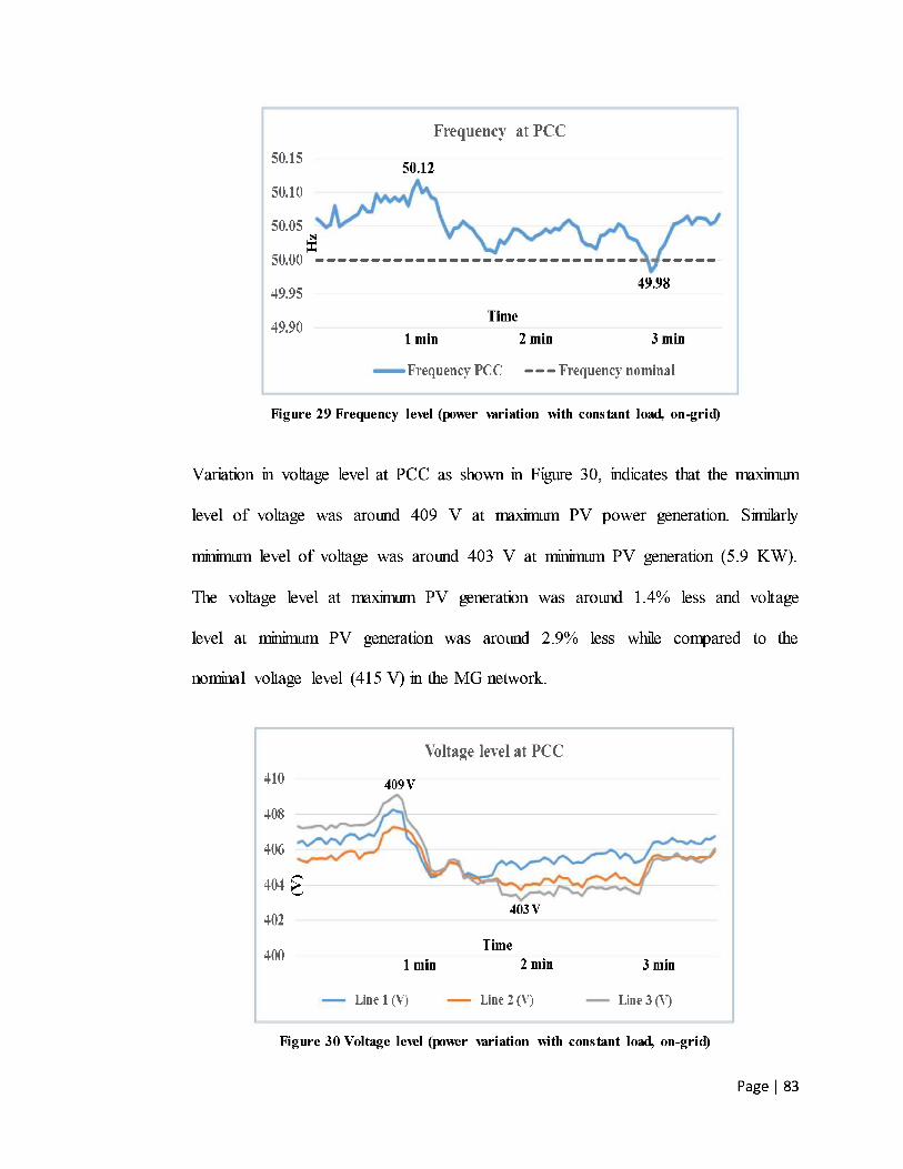
Page | 83
Figure 29 Frequency level (power variation with constant load, on - grid)
Variation in voltage level at PCC as shown in Figure 30 , indicates that the maximum
level of voltage was around 409 V at maximum PV power generation. Similarly
minimum level of voltage was around 403 V at minimum PV generation (5.9 KW).
The voltage level at maximum PV generation was around 1.4% less and volt age
level at minimum PV generation was around 2.9% less while compared to the
nominal voltage level (415 V) in the MG network.
Figure 30 Voltage level (power variation with constant load, on - grid)

Page | 84
4.5.1.2 Actual PV Power Variation with the constant Load: Off-Grid Mode
This analysis was carried out over the 6 minutes period with the integration of
rooftop solar PV and MT generator along with load bank in MG network at off-grid
condition. Figure 31 shows the MG network arrangement with the configuration of
load, Micro turbine, and solar PV for actual PV power variation and constant load
condition (off-grid).
Figure 31 MG configuration for voltage and frequency analysis (off-grid)
During this analysis, a real solar disturbance with frequent power variation in the
roof top solar PV was considered. During the solar disturbance (up to 2 minutes 40
sec), minimum and maximum level of power variation from connected solar PV was
observed around 17.3 KW to 24.6 KW respectively, as shown in Figure 32.
12.5 kW 12.5 kWLoad 31 kWMicro Turbine
30 kW
Roof top PV

Page | 85
Figure 32 Power level of PV (constant load, off - grid)
Figure 33 Power level of MT Generator (constant load, off - grid)
An integration of act ive power load (31 KW) was considered at constant level
throughout this analysis. Figure 33 shows the output power level of MT generator
varies from the minimum to maximum level of around 7 KW and 12.8 KW
respectively. Power sharing among the PV and MT gen erator along with the power
consumption from the connected load is shown in Figure 34 .
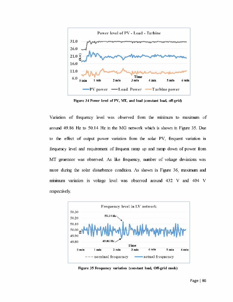
Page | 86
Figure 34 Power level of PV, MT, and load (constant load, off - grid)
Variation of frequency level was observed from the minimum to maximum of
around 49.86 Hz to 50.14 Hz in the MG network which is shown in Figure 35 . Due
to the effect of output power variation from the solar PV, frequent variation in
frequency level and requirement of frequent ramp up and ramp down of power from
MT generator was observed. As like frequency, number of voltage deviations was
more during the solar disturbance condition. As shown in Figure 36 , maximum and
minimum variation in voltage level was observed around 432 V and 404 V
respectively.
Figure 35 Frequency variation (constant load, Off - grid mode)

Page | 87
Figure 36 Voltage variation (constant load, off - grid mode)
4.5.1.3 Frequent Power Variation and Load Variation: On - Gri d
During this case study, MT generator with 30 KW rated capacity and 64 kVA load
bank were integrated in the MG network alon g with the grid source. MG network
configuration with inclusion of MT generator along with integration of load facility
is shown in Figure 37 .
12 minutes duration of typical power (generation) and load profile has been
considered for this analysis. A power profile of solar PV (25 KW ) followed by a
typical solar profile has been considered. The power profile with frequent variation
in power generation which is equivalent to a minute s level variation of solar
irradiance in a typical solar profile has been considered.

Page | 88
Figure 37 MG configuration (frequent power and load variation (on - grid)
Figu re 38 Typical Solar profile
The typical solar profile as shown in Figure 38 , clearly indicates that the maximum
solar irradiance was around 924 Watts/m2 and minimum irradiance was 0 Watts/m2
respectively. Similarly, a typical load profile as shown in Figure 39 clearly indicates
that the variation of load from maximum to minimum level was around 21.8 KW and
5.2 KW respectively. Power set point as per the varying power profile was given to
load controller of the MT generator. Similarl y, active power set point command was
given to load bank controller as per the typical varying load profile. Active power
output generation from the MT generator and power consumption from the load bank
is shown in Figure 40 .

Page | 89
Figure 39 Typical load profile
Figure 40 Active power of Micro Turbine and Load
As shown in Figure 41 , the maximum level of frequency at PCC was observed
around 50.12 Hz where the load was at minimum of around 10 KW and maximum
Turbine power of around 22 KW . Similarly, minimum level of frequency was
observed around 49.94 Hz while power generation was 0 KW and load was around
15 KW . Maximum and minimum deviation of frequency was around +0.12 Hz and
0. 06 Hz respectively while comparing to the nominal level (50 Hz ).

Page | 90
Figure 41 Frequency level at PCC (varying load, on - grid)
Figure 42 Voltage level at PCC (varying load, on - grid )
Voltage level at PCC varies according to the varying power and load condition in the
MG network is shown in Figure 42 . Maximum voltage level was observed around
412 V (4 minutes 47 sec) while power generation was at the maximum level (23
KW) and minimum load (10.29 KW) condition. Similarly, minimum voltage level
was observed around 405 V (11 minutes 50 sec) while there is no power generation
(0 KW) and maximum load (19.46 KW) condition. As compared to the nominal
voltage (415 V) level, the voltage level at maximum power generation and minimum

Page | 91
load condition was around 0.7% less and voltage level at no power generation and
maximum load condition was around 2.4% less at PCC point of MG network.
Results of frequency and voltage variation level during “on-grid” and “off-grid”
mode of MG operation is given in Table 12 and Table 13respectively.
Table 12 Frequency variation (Hz)
MG mode Conditions Frequency variation (Hz)
Actual (max)
Actual (min)
w.r.t (50 Hz) (max)
w.r.t (50 Hz) (min)
On-grid
Power variation (with constant load)
50.12 49.98 0.12 - 0.02
Frequent Power variation (with load variation) 50.12 49.94 0.12 - 0.06
Off-grid Power variation (with constant load)
50.14 49.86 0.14 - 0.14
w.r.t (50 Hz) is the with respect to nominal frequency
Table 13 Voltage variation (% )
MG mode Conditions Voltage variation (V)
Actual (max)
Actual (min)
w.r.t (VN) (max) %
w.r.t (VN) (min) %
On-grid
Power variation with constant load
409 403 - 1.4 - 2.8
Frequent Power variation with load variation
412 405 - 0.72 - 2.4
Off-grid Power variation with constant load 432 404 + 4.1 - 2.7
w.r.t (VN) is the with respect to nominal voltage (415 V)
The voltage and frequency variation results from the on-grid mode of analysis were
observed to be minimal and within the tolerance limit as per the AS 60038 and
Australian network standard (NEM). This is because, MG is connected with infinite
power source called grid source which can maintain better voltage and frequency
regulation in the MG network easily. As compared to the results from the on-grid
mode of analysis, variation in voltage and frequency level was high in the off-grid
mode. This is due to the low inertia characteristics of islanded MG network.
However maximum and minimum variation in frequency level was maintained close
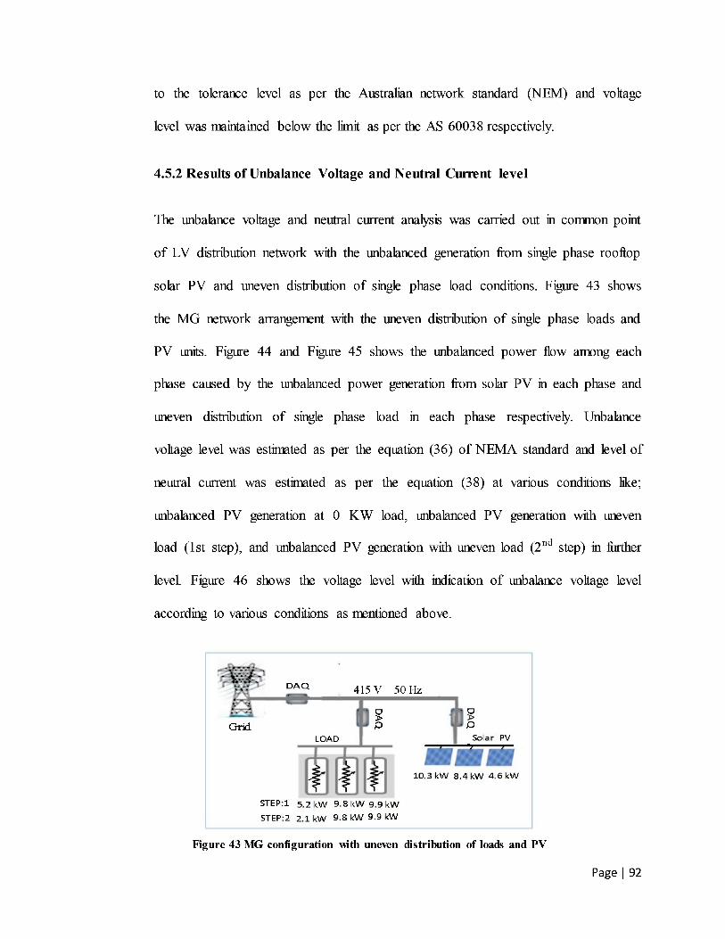
Page | 92
to the tolerance level as per the Australian network standard (NEM) and voltage
level was maintained below the limit as per the AS 60038 respectively.
4.5.2 Results of U nbalance Voltage and Neutral Current level
The u nbalance voltage and neutral current analysis was carried out in common point
of LV distribution network with the unbalanced generation from single phase rooftop
solar PV and uneven distribution of single phase load conditions. Figure 43 shows
the MG network arrangement with the uneven distribution of single phase loads and
PV units. Figure 44 and Figure 45 shows the unbalan ced power flow among each
phase caused by the unbalanced power generat ion from solar PV in each phase and
uneven distribution of single phase load in each phase respectively. Unbalance
voltage level was estimated as per the e quation (36 ) of NEMA standard and level of
neutral current was estimated as per the e q uation (38 ) at various conditions like;
unbalanced PV generation at 0 KW load, unbalanced PV generation with uneven
load (1st step), and unbalanced PV generation with uneven load (2nd step) in further
level. Figur e 46 shows the voltage level with indication of unbalance voltage level
according t o various conditions as mentioned above.
Figure 43 MG configuration with uneven distribution of loads and PV
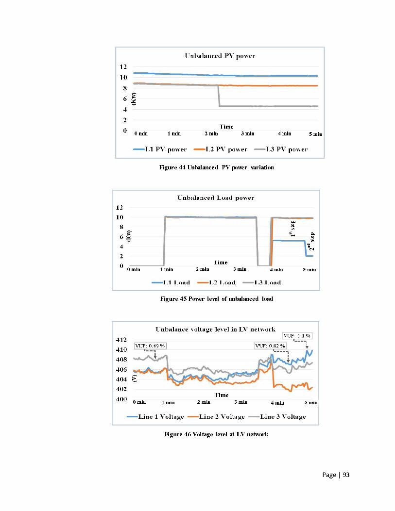
Page | 93
Figure 44 Unbalanced PV power variation
Figure 45 Power level of unbalanced load
Figure 46 Voltage level at LV network
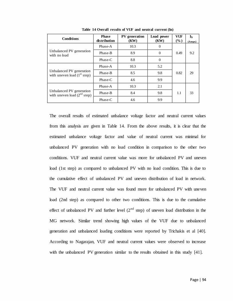
Page | 94
Table 14 Overall results of VUF and neutral current (In)
Conditions Phase
distribution PV generation
(KW) Load power
(KW) VUF (% )
IN
(Amps)
Unbalanced PV generation with no load
Phase-A 10.3 0
0.49 9.2 Phase-B 8.9 0
Phase-C 8.8 0
Unbalanced PV generation with uneven load (1st step)
Phase-A 10.3 5.2
0.82 29 Phase-B 8.5 9.8
Phase-C 4.6 9.9
Unbalanced PV generation with uneven load (2nd step)
Phase-A 10.3 2.1
1.1 33 Phase-B 8.4 9.8
Phase-C 4.6 9.9
The overall results of estimated unbalance voltage factor and neutral current values
from this analysis are given in Table 14. From the above results, it is clear that the
estimated unbalance voltage factor and value of neutral current was minimal for
unbalanced PV generation with no load condition in comparison to the other two
conditions. VUF and neutral current value was more for unbalanced PV and uneven
load (1st step) as compared to unbalanced PV with no load condition. This is due to
the cumulative effect of unbalanced PV and uneven distribution of load in network.
The VUF and neutral current value was found more for unbalanced PV with uneven
load (2nd step) as compared to other two conditions. This is due to the cumulative
effect of unbalanced PV and further level (2nd step) of uneven load distribution in the
MG network. Similar trend showing high values of the VUF due to unbalanced
generation and unbalanced loading conditions were reported by Trichakis et al [40].
According to Nagarajan, VUF and neutral current values were observed to increase
with the unbalanced PV generation similar to the results obtained in this study [41].
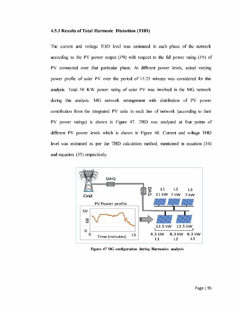
Page | 95
4.5.3 Results of Total Harmonic Distortion (THD)
The current and voltage THD level was estimated in each phase of the network
according to the PV p ower output ( P 0) with respect to the full power rating ( Pr ) of
PV connected over that particular phase. At different power levels, actual varying
power profile of solar PV over the period of 15.25 minutes was considered for this
analysis. Total 50 KW power rating of solar PV was involved in the MG network
during this analysis. MG network arrangement with distribution of PV power
contribution from the integrated PV units in each line of network (according to their
PV power ratings) is shown in Figure 47 . THD was analyzed at four points of
different PV power levels which is shown in Figure 48 . Current and voltage THD
level was estimated as per the THD calculation method, mentioned in equation ( 3 4 )
and equation ( 3 5 ) respectively.
Figure 47 MG configuration during Harmonics analysis
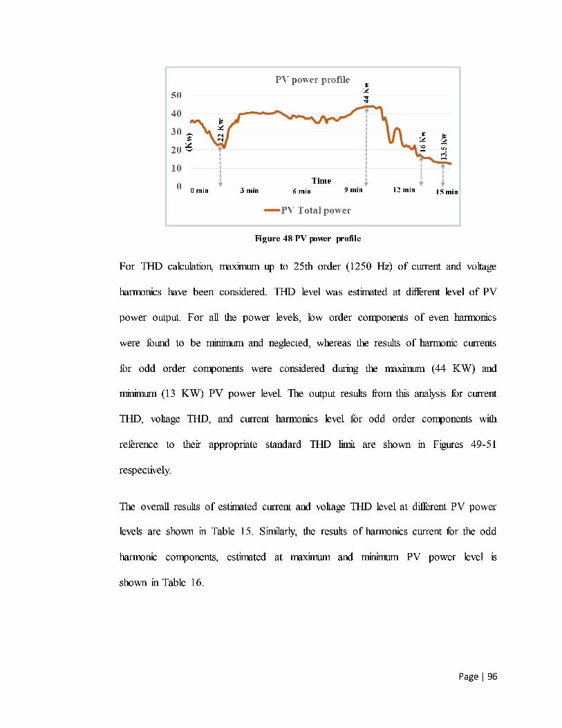
Page | 96
Figure 48 PV power profile
For THD calculation, maximum up to 25th order (1250 Hz) of current and voltage
harmonics have been considered. THD level wa s estimated at different level of PV
power output. For all the power levels, low order components of even harmonics
were found to be minimum and neglected, whereas the results of harmonic currents
for odd order components were considered during the maximum (44 KW) and
minimum (13 KW) PV power level. The output results from this analysis for current
THD, voltage THD, and current harmonics level for odd order components with
reference to their appropriate standard THD limit are shown in Figures 49 - 51
respecti vely.
The overall results of estimated current and voltage THD level at different PV power
levels are shown in Table 1 5 . Similarly, the results of harmonics current for the odd
harmonic components, estimated at maximum and minimum PV power level is
shown i n Table 16 .

Page | 97
Figure 49 Current THD at different level of PV power
Figure 50 Voltage THD at different level of PV power
Figure 51 Current THD of odd ha rmonics

Page | 98
Table 15 Results of THD level at different PV power level
Phases P0 (KW)
P0 / Pr (% )
Current THD (% )
Voltage THD (% )
Line 1
16.6 86 2.4 1.6
8 41 4.2 1.9
6 31 4.8 1.95
5 26 5.7 2.6
Line 2
13.7 89 1.9 1.6
7 46 3.9 1.7
5 33 4.9 1.85
4.3 28 5.1 1.9
Line 3
13.7 89 1.9 1.5
7 46 4.1 1.8
5 33 4.6 1.9
4.2 28 4.9 2.5
Table 16 Results of odd harmonics at different PV power level
Odd harmonics
Current THD (% ) at Min PV power
Voltage THD (% ) at Max PV power
Line 1 Line 2 Line 3 Line 1 Line 2 Line 3
3rd order 1.2 1.7 1.7 1 0.7 0.6
7th order 3.9 3.8 2.8 1.7 1.4 1.3
11th order 3.3 1.2 1.8 1.3 1.1 1.2
13th order 2.2 2.2 2 1.2 0.9 0.5
In all the cases, voltage THD level (Figure 50, Table 15) was found to be minimum
and within the tolerance level of AS/NZS 61000.2.2 standard. At 86% of maximum
PV power level (P0/Pr) in phase-A, and 89% in other two phases (phase-B and
phase-C), the current THD (Figure 51, Table 15) was found to be minimum of
around 2.4% in phase-A, and 1.9% in phase-B and phase-C respectively. At 26% of
minimum PV power level in phase-A, and 28% in other two phases (phase-B and

Page | 99
phase-C), the current THD level was found to be high in phase-A (5.7%), phase-B
(5.2%) which exceeds the THD limit and current THD in phase-C (4.9%) was found
close to the THD tolerance level as per the AS 4777 standard.
Results from the Table 16 clearly indicate that the current harmonics in odd order
component was high at minimum PV power level (P0/Pr) as compared to the
maximum power level. At minimum PV power level, current harmonics in 7th order
for phase-A (3.9%) and phase-B (3.8%) was found to be high and close to the THD
tolerance level and current harmonics in 13th order for phase-A and phase-B (2.2%)
was found to be above the THD limit as per the AS4777 standard.
Finally, based on the results from this analysis, it can be concluded that the current
THD level was high at minimum PV power level (P0/Pr) and low at maximum PV
power level (P0/Pr). This is due to the influence of fundamental current magnitude
(based on the generated PV power output) over the harmonic currents of PV inverter.
The results on current THD level from the experimental analysis follow the same
trend as that of Valentina et al and the reason for high current THD level during
minimum PV power condition was due to the cloud effect [39].
4.6 Conclusion
In this study, the PQ issues like frequency and voltage variation, unbalance voltage
and neutral current level, and THD level were analyzed and quantified in LV
network of the MG power system through an experimental approach in the presence
of real cloud effect and other scenarios.

Page | 100
Based on the results obtained, it was found that
Voltage/frequency level in the on-grid and islanded MG network was greatly
affected by the transient conditions (change in the load and PV output power
variation) and the real cloud effect with the significant variation observed in
both the parameters. This has not been reported before as per the author‟s
knowledge.
Variation of voltage/frequency level in the off-grid mode was higher than the
on-grid mode. This gives clear information on the behavior of islanded MG
network in presence of the actual cloud effect/ load change conditions. This
will be helpful to take compensating control measures to minimize the
variation level in such conditions.
Unbalance voltage (VUF) and neutral current level were found to increase
with the increase in unbalanced PV generation and uneven load in the MG
network.
Overall current THD and individual odd order current THD level in the MG
network was found to be greatly affected by the different PV power levels
caused by the real cloud effect. This is a significant finding, because in
previous works THD level was shown to be affected mostly by the different
PV penetration levels (with respect to the load).

Page | 101
Chapter 5
Power Management and Power Sharing Control of Solar PV MG
5.1 Introduction
In the previous chapters, the effect of multiple scenarios on the PQ factors of the PV
based MG network was explored through simulation and experimental approach.
As highlighted in the Section 2.5, due to the intermittent nature of the PV, additional
DG source like battery storage is required in the PV based MG network. It was also
mentioned in the Section 2.7 that during the on-grid and off-grid mode of MG
operation, maintaining power balance is essential to obtain better regulation of the
voltage/frequency level in the MG network through the implementation of a co-
ordinated power management and power sharing control strategy.
Thus in this work, a PV based MG network integrated with battery storage was
developed in MATLAB-SIMULINK, co-ordinated power management and power
sharing control (modified droop control) strategy was implemented and the PQ
analysis was carried out in on-grid, off-grid and on-grid to off-grid transition mode
with varying load and varying solar irradiance condition. GsGfm type VSI was
chosen for the PV units and battery in the MG network due to its advantages
mentioned in the Section 2.6.3 over the grid-feeding and grid-forming type VSI used
in the previous research works.

Page | 102
The effectiveness of using the GsGfm type VSI in the developed MG model will be
assessed from the variation in PQ factors like voltage/frequency and power level
during the on-grid to off-grid transition mode particularly, whether smooth operation
of the MG is ensured.
Content of this chapter has been published in the Journal of “Smart Grid and
Renewable Energy”, (volume 8; Number 1 (January 2017); pp 1-30), Scientific
Research Publishing Inc.
This chapter is organized as follows; Section 5.2 describes the MG model
configuration includes the specification of MG elements along with detail of DC
power converters for solar PV and battery storage, Section 5.3 presents the control
configuration detail of GsGfm type VSI, used for PV and battery storage, Section 5.4
describes the power management control strategies for on-grid and off-grid mode of
the MG operation, Section 5.5 demonstrates the type of analysis and results
discussion, and Section 5.6 concludes the outcomes from this study.
5.2 MG Model Configuration
The configuration of a typical AC MG network model which is operating at voltage
and frequency level of 400 V and 50 Hz is shown in Figure 52. The specification
details of DC equipment, LV load/feeder, and DC equipment included in the MG
network are given in Table 17, Table 18, and Table 19 respectively.
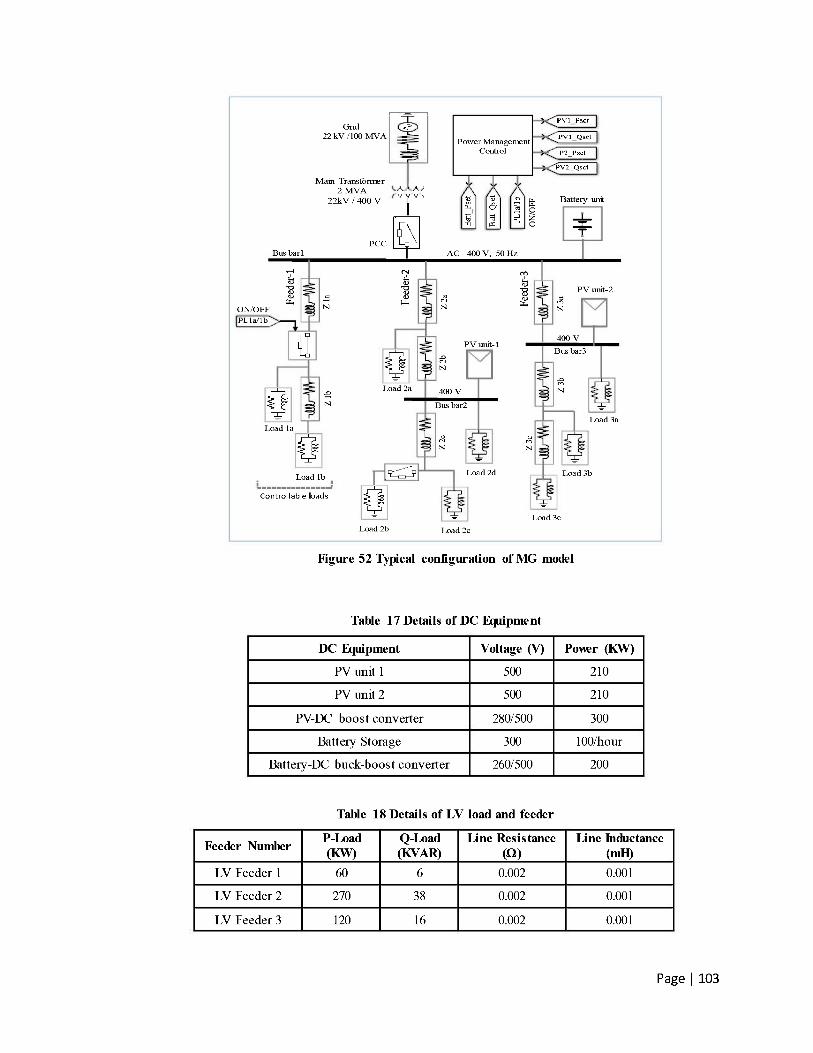
Page | 103
Figure 52 Typical co nfiguration of MG model
Table 17 Details of DC Equipment
DC Equipment Voltage (V) Power (KW)
PV unit 1 500 210
PV unit 2 500 210
PV - DC boost converter 280/500 300
Battery Storage 300 100/hour
Battery - DC buck - boost converter 26 0/500 200
Table 18 Details of LV load and feeder
Feeder NumberP - Load(KW)
Q - Load(KVAR)
Line Resistance( )
Line Inductance(mH)
LV Feeder 1 60 6 0.002 0.001
LV Feeder 2 270 38 0.002 0.001
LV Feeder 3 120 16 0.002 0.001

Page | 104
Table 19 Details of AC Equipment
AC Equipment Rating (MVA) Voltage (KV)
Grid Source – Short Circuit Capacity 100 22
Main Transformer 2 22/0.4
PV Inverter 0.3 0.26
PV Inverter Interfacing Transformer 0.3 0.26/0.4
Battery Inverter 0.2 0.26
Battery Inverter Interfacing Transformer 0.3 0.26/0.4
5.2.1 Solar PV unit and DC Power converter
In this proposed MG model, Solar PV unit includes two stages of power converters;
DC-DC boost converter and DC-AC Voltage Source Inverter (VSI). A typical solar
PV unit has been considered with the maximum power generation capacity of around
210 KWp at standard test condition (STC). Each PV module open circuit voltage
(VOC) and short circuit current (ISC) were 64.2 V and 5.36 Amps respectively.
Maximum power generation and I-V characteristics curve of the proposed solar PV
unit at different solar irradiance conditions are shown in Figure 53 and Figure 54
respectively.
Figure 53 PV unit PV curve (Power versus Voltage)
50 100 150 200 250 300 35000
100
150
200
210
VOLTAGE (V)
POW
ER (
kW
)
50

Page | 105
Figure 54 PV unit I-V curve
The DC-DC boost power converter is widely used for the solar PV unit which
amplifies and regulates the PV array voltage into specified level along with the
extraction of maximum power from PV array as per the maximum power point
tracking (MPPT) control algorithm. Implementation of the MPPT control algorithm
in the DC converter, varies duty cycle of the converter according to maximum power
condition [119, 120]. In this proposed MG model, Perturb and observe (PO) MPPT
control algorithm has been implemented for the DC converter of PV unit which
boosts up PV array voltage (280 V) into 500 V as the nominal level at inverter input.
5.2.2 Battery storage and Bi-directional DC Power converter
The battery storage plays a major role in the PV based MG network, where it
compensates power variation of the solar PV and maintain the power balance
between generation and consumption. It ensures better voltage and frequency
regulation, power support for critical loads in the MG network during stand-alone
condition. It also improves the power quality, stability of distribution network and
fulfills the various demand side management functions like; load leveling, peak
shaving, etc. [45, 46]. In this study, a storage unit has been considered as a
50 100 150 200 250 300 35000
400
600
800
1000
VOLTAGE (V)
CU
RR
EN
T
(AM
PS
)
200

Page | 106
parameterized generic model of lead acid battery which is readily available in the
MATLAB-SIMULINK library. Operating voltage (V) and Ampere-hour (Ah)
capacity of the lead acid battery unit has been considered around 300 V and 340 Ah
respectively. Battery discharge curve which is drawn on the basis of battery voltage
and Ah capacity is shown in Figure 55.
Figure 55 Battery discharge curve
The DC buck-boost converter which is called as bidirectional converter is widely
used to interface battery storage unit in the DC side. DC bidirectional converter
mainly consists of two IGBT switches, out of that one switch allows battery
operation in buck mode while charging and other switch allows in boost mode while
discharging condition [48, 121]. In this proposed MG model, bidirectional DC
converter of battery unit has been considered to operate in the voltage level of
around 300 V in the buck side to 500 V in the boost side. In this study, central power
management determines the charge and discharge operation of battery according to
the following conditions; availability of PV power generation/load condition in the
MG network and SOC level of battery. In order to avoid the battery from overcharge
220
240
260
280
300
320
0 50 100 150 200 250 300 350AMPERE-HOUR (Ah)
VO
LTA
GE
(V
)
NORMAL OPERATING AREA

Page | 107
and under discharge condition, the SOC control in power management allows the
battery to operate within safe SOC operating range (30 % to 80 %).
In this study, Grid-support Grid-forming (GsGfm) type VSI has been considered
for PV and battery storage in the proposed LV network of MG model. Control
configuration of VSI which is developed according to the resistive nature of LV
network has been discussed in detail in the following section.
5.2.3 Control configuration of GsGfm type VSI for the developed MG model
The overall control configuration of VSI used for the PV units and battery storage
in this proposed LV network of the MG model is shown in Figure 56. The control
configuration chosen for GsGfm type VSI was based on [66, 67] and the concept
has already been discussed in the Section (2.6.3.1) of Chapter 2. Previous research
work on PV based MG network either used grid-feeding or grid-forming type VSI
in which the former can be operated in grid connected mode and later is suitable
to be operated in the island or off-grid mode [65, 66]. The main difference between
the present model in the study and previous researchers work is the use of GsGfm
type VSI in the PV based MG network which has the ability to operate in both the
on-grid and island mode without changing its control configuration. In addition,
due to the resistive nature of LV network in the proposed MG model of this study,
a modified droop control strategy with implementation of virtual resistor in virtual
impedance control loop have been considered for the proposed VSI control
configuration. Figure 57 shows the detailed control configuration of modified
droop controller along with the power calculation block. Figure 58 shows the

Page | 108
control configuration of voltage and current control loop with inclusion of virtual
resistor in the virtual impedance control loop .
Figure 56 Overall control configuration of VSI [88,89]
Figure 57 Power calculation block with modified droop control
Figure 58 Configuration of voltage and current control

Page | 109
5.2.3.1 Modified droop control loop (for LV network)
On contrary to inductive nature of the HV network, in low voltage (LV) network
where the line impedance is in resistive nature, the active power (P) can be
controlled by the voltage magnitude (V) and reactive power (Q) can be regulated by
controlling the power angle (δ) of network [66, 72, 74]. Active (P) and reactive (Q)
power flow in LV network can be expressed as per the equations (39) and (40)
respectively:
P =
, (39)
Q =
δ, (40)
where V1 is the inverter output voltage magnitude, V2 is the voltage magnitude of
PCC network, X is the line impedance (resistance), and δ is the power angle.
Considering the expression of power flow equations in (39) and (40), power droop
control strategies in the LV network can be expressed as per the equations (41) and
(42) respectively. In contrary to conventional P-f and Q-V droop control, modified
P-V and Q-f droop control which is known as opposite droop control is commonly
used for the LV network [66, 68, 72]:
ω** = ωn + KQ (Qref – Q), (41)
E** = Vn – KP (Pref – P), (42)
KP =
, (43)
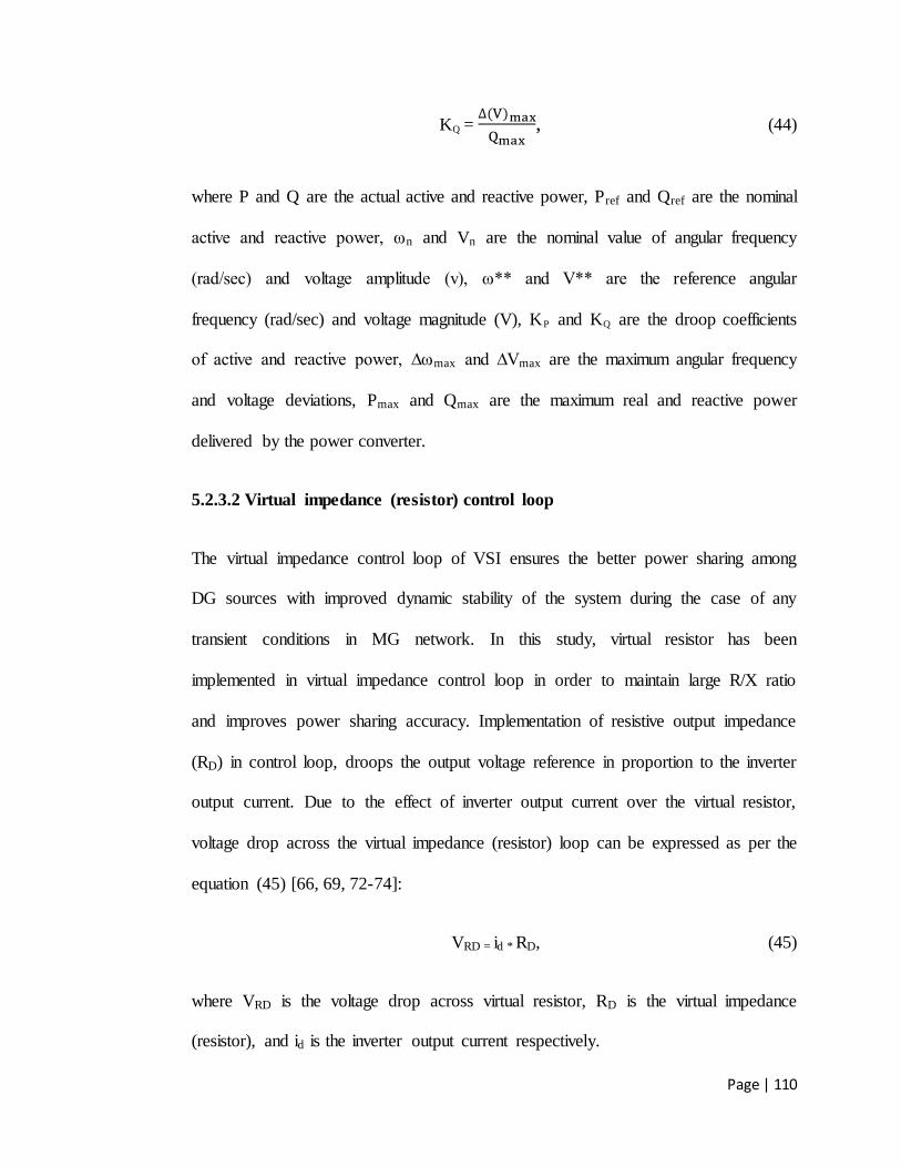
Page | 110
KQ =
, (44)
where P and Q are the actual active and reactive power, Pref and Qref are the nominal
active and reactive power, ωn and Vn are the nominal value of angular frequency
(rad/sec) and voltage amplitude (v), ω** and V** are the reference angular
frequency (rad/sec) and voltage magnitude (V), KP and KQ are the droop coefficients
of active and reactive power, ∆ωmax and ∆Vmax are the maximum angular frequency
and voltage deviations, Pmax and Qmax are the maximum real and reactive power
delivered by the power converter.
5.2.3.2 Virtual impedance (resistor) control loop
The virtual impedance control loop of VSI ensures the better power sharing among
DG sources with improved dynamic stability of the system during the case of any
transient conditions in MG network. In this study, virtual resistor has been
implemented in virtual impedance control loop in order to maintain large R/X ratio
and improves power sharing accuracy. Implementation of resistive output impedance
(RD) in control loop, droops the output voltage reference in proportion to the inverter
output current. Due to the effect of inverter output current over the virtual resistor,
voltage drop across the virtual impedance (resistor) loop can be expressed as per the
equation (45) [66, 69, 72-74]:
VRD = id * RD, (45)
where VRD is the voltage drop across virtual resistor, RD is the virtual impedance
(resistor), and id is the inverter output current respectively.

Page | 111
5.2.3.3 Voltage and current control loop of VSI
The PI based voltage control loop of VSI which is used for PV units and battery
storage in this proposed MG model is same as the voltage controller of GsGfm type
VSI, discussed in the Section (2.6.3.1) of chapter 2. Considering the effect of virtual
resistor output voltage, expression of output reference currents from the voltage
controller can be written as per the equations (47) and (48) respectively:
Vref (N) = (E** - VRD), (46)
Id-ref = (Vref (N) – Vd)
(47)
Iq-ref = – (Vq + VRD)
(48)
where VRD is the output voltage of virtual resistor, E** is the voltage reference signal
from droop controller, Vref (N) is the new voltage reference signal after the subtraction
of VRD from E**, id-ref and iq-ref are the output reference current components from the
voltage controller, Vd and Vq are the voltage components in d-axis and q-axis, Kp
and Ki are the proportional and integral gain of PI controller.
In this study, in order to enhance the stability of PI based current controller that the
decoupling operation through current feed forward compensation has been adopted
by considering inverter reference currents (id-ref, iq-ref) instead of output measured
currents (id, iq) [66, 78]. As per the control configuration of current control loop with
the inclusion of feed forward voltage and inverter reference current feed forward

Page | 112
facility, output voltage signals from the current control loop of VSI can be expressed
as follows:
[
] = [
] [
] + [
] [
] + [
] [
] + [
] , (49)
= (id-ref – id);
= (iq-ref – iq),
where Ud and Uq are the output voltage signal in d-q form, ω is the angular frequency
of network, L is the inductance between inverter and PCC network, Vd is the d-axis
voltage component, Vq is the q-axis voltage component, Id and Id-ref are the d-axis
actual and reference current component, Iq and Iq-ref are the q-axis actual and
reference current component, Kp and Ki is the proportional and integrator gain of PI
controller. Thus in this study, in order to get better power sharing among DG sources
in the proposed LV network (R/X ratio 6.37) of MG model, a modified droop control
with implementation of virtual resistor in virtual impedance control loop have been
considered for the control configuration of GsGfm type inverter. Main parameters of
VSI are given in the Table 20.
Table 20 Inverter control and system parameters
Description Parameter Value
Inverter nominal frequency (ωn) Rad/sec 314
Inverter output Filter Inductance (L) mH 0.25
Inverter output Filter Capacitance (C) μF 480
Virtual output resistor (RD) Ω 0.01
Inverter nominal voltage (Vn) V 260
Voltage droop gain (KV) V/VAR 0.0005
Frequency droop gain (Kω) Rad/s W 0.006
Inverter switching frequency (fS) KHz 1.6

Page | 113
In order to get a power balance between the generation and consumption, and
coordinated operation between solar PV and battery storage, power management
control strategies have been developed and implemented in this proposed MG model.
Details of the Power management control strategies, developed for on-grid and off-
grid mode of the MG operation has been discussed in the following section.
5.3 Power management control strategies
Various power management control strategies have been developed and utilized to
maintain power balance and co-ordinated control operation between DG sources in
the islanded as well as grid connected MG network [45, 81, 82, 122]. The control
logics for developing power management strategy can vary according to the type of
MG model configuration and type of equipment‟s used in the MG network. Power
management control strategy developed and implemented for the proposed MG
model operating in on-grid and off-grid mode was based on the works of previous
researchers [45, 81, 82, 122]. The purpose of the proposed control strategy was to
ensure power balance and co-ordinated control operation between PV units and
battery storage in the MG network.
During the on-grid mode, both PV units were allowed to operate in the maximum
power generation irrespective of load condition in the MG network. Battery storage
was allowed to charge in case of low demand and excess PV power generation or
during the case of power export to the grid reaches certain level. Similarly, battery
storage was allowed to discharge in case of high demand and excess power import
from the grid network. However during off-grid mode, both PV units were allowed

Page | 114
to curtail their power generation according to load condition in the network. Battery
storage was allowed to charge in case of excess PV power generation and low
demand condition. Similarly, in case of power demand reaches above the maximum
power generation for both the PV units, the battery storage was allowed to discharge
in appropriate level. Power management control also includes a battery State of
Charge (SOC) control which allows the battery to charge and discharge according to
allowable range of its SOC condition.
5.3.1 PV Power Management (on-grid)
During the on-grid mode, grid source act as a main power source which buffers any
deficit or excess power generation in the MG network. Both PV units were allowed
to operate at maximum power generation like the P-Q control method. Active power
set (Pset) of each PV unit was assigned to be 100% of its nominal power capacity
(210 KW) irrespective of the active power demand (PL) and reactive power set
(Qset) of each PV unit which was assigned to be 40% of total current reactive power
demand (QL) in the MG network. Figure 59 shows the detail of the PV power
management with assigned power set values.
Figure 59 PV Power Management (on-grid)
PV2_Pset
PV2_Qset
PV2 Active Power Set (100% of P_NOM) 1
PV2 Reactive Power Set (Max 40% 0f QL) 0.4 QL
PV1_Pset
PV1_Qset
PV1 Active Power Set (100% of P_NOM) 1
PV1 Reactive Power Set (Max 40% 0f QL) 0.4 QL

Page | 115
During on-grid mode, total active (P) and reactive (Q) power contribution from both
PV units can be expressed as per the equations (50) and (51) respectively.
Expression of active (P) and reactive (Q) power balance in MG network can be
written as per the equations (52) and (53) respectively:
P(PV) = (P(NOM)) [P(PV1) + P(PV2)], (50)
Q(PV) = (0.4QL) [Q(PV1) + Q(PV2)], (51)
PL + P(Loss) = P(PV) + P(PG) +/- PB, (52)
QL + Q(Loss) = Q(PV) + Q(PG) + QB, (53)
where P(PV) was the total active (P) power contribution from both PV units, P(PV1)
and P(PV2) was the active power generation of PV1 and PV2, Q(PV) was the total
reactive (P) power contribution from both PV units, Q (PV1) and Q(PV2) was the
reactive power generation of PV1 and PV2, PL and P(Loss) was the total active power
load and active power losses, QL and Q(Loss) was the total reactive power load and
reactive power losses, P(PG) and Q(PG) was the active and reactive power of grid
source, PB and –PB was the charging and discharging active power of battery and QB
was the reactive power (discharge) of battery respectively.
5.3.2 Battery power management with inclusion of SOC control (on-grid)
The battery power management includes a three part of control strategy namely;
Active power (P), Reactive power (Q), and State of Charge (SOC) control of battery.
The control logics of active (P) and reactive (Q) power management for the battery
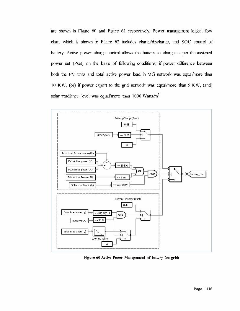
Page | 116
are shown in Figure 60 and Figure 61 respectively. Power management logical flow
chart which is shown in Figure 62 includes charge/discharg e, and SOC control of
battery. Active power charge control allows the battery to charge as per the assigned
power set (Pset) on the basis of following conditions; if power difference between
both the PV units and total active power load in MG network was equal/more than
10 KW , (or) if power export to the grid network was equal/more than 5 KW , (and)
solar irradiance level was equal/more than 1000 Watts/m2.
Figure 60 Active Power Management of battery (on - grid)

Page | 117
Figure 61 Reactive Power Management of battery (on - grid)
Figure 62 Flow chart for power management of battery (on - grid)
Reactive power management control enables the battery to discharge as per the
assigned reactive power set (Qset) with the following conditions; if sum of the
reactive power cont ribution from both the PV units were more than 26 KVAR, (or)
reactive power import from the grid network was more than 10KVAR, (and) total

Page | 118
reactive power demand was more than 45KVAR in MG network.
Figure 63 Look-up table for battery discharge (2nd level)
Similarly, based on the solar irradiance level, the battery discharge control strategies
were developed in two levels. In the first level, battery was allowed to discharge as
per the assigned power set (Pset) when the solar irradiance level was equal/more than
990 Watts/m2. In second level, if solar irradiance level reaches below the first level
(990 Watts/m2), the battery discharge power control follows a look-up table curve
which is shown in Figure 63. As per look-up table curve, battery allows discharge by
discharge control when the solar irradiance of PV unit varies as below 990 Watts/m2.
This is to ensure smooth out or compensating the power variation of PV in case of
any disturbance in solar irradiance condition.
The SOC control ensures safe operation of the battery by allowing battery to operate
between the safe ranges (30% to 80%) of SOC level. In order to avoid over charge
and under discharge condition of battery, SOC control stops battery from charging
while SOC reaches equal/above 80% (maximum), similarly it stops from
discharging, while SOC reaches equal/below 30% (minimum).
Dis
char
ge(P
set)
1000950900850800750700
0.1
0.2
0.15
0.25
0.30
0.35
0.40
0.45
0.50
0.55
Solar Irriadiance - Watts/m2

Page | 119
5.3.3 Power management of PV units (off-grid)
In the off-grid mode, inverters of the PV units were operating as voltage source
which provides active and reactive power support according to the voltage and
frequency level in the MG network. Battery storage provides active and reactive
power support according to the power generation level of PV and power demand in
the MG network. Therefore, power management in off-grid mainly involves the
battery power management with the inclusion of SOC control. In addition, load
management control strategy was implemented for a safe and reliable operation of
the PV based MG.
During off-grid mode, active (P) and reactive (Q) power balance in MG network can
be expressed as per the equations (54) and (55) respectively:
PL + P(Loss) = [P(PV1) + P(PV2)] +/- PB, (54)
QL + Q(Loss) = [Q(PV1) + Q(PV2)] + QB, (55)
where P(PV1) and P(PV2) is the active power generation of PV1 and PV2, Q (PV1) and
Q(PV2) is the reactive power generation of PV1 and PV2, PL and P(Loss) is the total
active power load and active power losses, QL and Q (Loss) is the total reactive power
load and reactive power losses, PB and –PB is the charging and discharging active
power of battery, QB is the reactive power (discharge) of battery.
5.3.4 Battery power management (off-grid)
The control configuration of the battery active power (P) management with inclusion
of SOC load management control and reactive power (Q) management of the battery

Page | 120
storage are shown in Figure 64 and Figure 65 respectively. The logical control flow
chart which includes power and load management control of battery is shown in
Figure 66.
In the off-grid mode, active power management control initiates the battery control
into charging mode, if the total active power load (PL) in the MG network was less
than the maximum power capacity of both the PV units. In addition, charge control
continues to allow battery to charge with the following conditions; if PV unit output
power generation was less than 95% (200 KW) of its nominal power capacity and
solar irradiance level should be equal/more than 1000 Watts/m2. Similarly, if both
PV units were in maximum power generation (above 400KW) and total active power
load in the MG network was more than both the PV capacities, the battery active
power discharge control allows battery to discharge in the appropriate level.
Similarly, if reactive power contribution of both PV units were less than total
reactive power load (QL) in the MG network, the reactive power management
control allows battery to discharge reactive power in the appropriate level.

Page | 121
Figure 64 Activ e power management of battery (off - grid)
Figure 65 Reactive Power Management of battery (off - grid)

Page | 122
Figure 66 Flow chart for Power management of battery (off - grid)
5.3.4.1 SOC control and Load power management (off - grid)
The SOC control behavior was similar to that of the on - grid power management,
stops battery from charging while SOC reaches equal/above the 80% and stops from
discharging while SOC reaches equal/below 30%. In addition, whenever SOC le vel
reaches to equal/below 30% and each PV unit power generation was more than 90%
(190 KW ) of its nominal power capacity, the load management control strategy
switch off feeder - 1 loads which were consid ered as the non - critical loads.
In this proposed MG m odel, power management control strategies was developed
and implemented in order to get a better power balance and coordinated control
operation between the PV and battery storage while MG was operating in both the

Page | 123
on-grid and off-grid mode. In addition, a better voltage and frequency regulation and
power sharing among DG sources in the MG network was guaranteed by means of
implementing modified droop with the virtual output impedance control for GsGfm
VSI of PV and battery storage. Effectiveness of control strategies were verified
through the model simulation in MATLAB-SIMULINK while varying solar
irradiance of PV and varying load conditions in the LV network of MG power
system. Through this study, regulation in voltage and frequency level, coordinated
power sharing among the PV units and battery storage, and harmonic distortions in
the MG network were analyzed in the following mode of MG operation like; on-grid,
off-grid, and on-grid to off-grid transition mode. Methodology and outcome from
this analysis are discussed in detail in the following sections.
5.4 Model analysis and results
In order to verify effectiveness of the control strategies in the proposed MG model
network, simulation and detailed analysis were carried out at different MG modes
like; on-grid, off-grid, and on-grid to off-grid transition.
5.4.1 On-grid mode Analysis
In the on-grid mode, both PV units were allowed to operate in the P-Q control mode
and battery storage was allowed to charge and discharge according to the availability
of PV power generation with respect to power demand in the MG network, solar
irradiance level, and amount of power flow to the grid network. During this analysis,
voltage and frequency level in the MG network, power sharing among the PV units,
battery storage and grid source were analyzed with the varying solar irradiance and

Page | 124
load conditions.
Varying load: During this analysis, load variation was set to 2 stages in the
MG network.as follows:
(a) 1st stage (2 sec), load was increased from 300 KW/30 KVAR into 370
KW/40 KVAR
(b) At 2nd stage (4 sec), it was further increased to 450 KW/50 KVAR.
Varying Solar irradiance: PV1 power was varied from 210 KW to 150 KW
(2.5 sec to 3.5 sec) due to the variation of solar irradiance from maximum
(1000 watts/m2) to minimum level (745 watts/m2).
5.4.1.1 Results and Discussion (On-grid)
The active (P) and reactive (Q) power contribution from the PV units, battery
storage, and grid source, observed during the varying load and varying solar
irradiance of PV1 in the MG network are shown in Figure 67.

Page | 125
Figure 67 Power sharing among the power sources and load (on - grid)
Throughout the on - grid analysis mode, the active power management control ensures
Active power generation for both PV1 and PV2 to be around 210 KW , w ith
the exception of PV1 decreasing from 210 KW during the variation of solar
irradiance condition ( Figure 67 ).
Battery storage to charge to a maxi mum of around 50 KW during excess ive
PV power generation/low demand and to discharge to a maximum of around
5 0 KW when the total power demand exceeds maximum power generation of
both PV units in the network. In order to avoid excess ive power import from
the grid network, the active power management control enables the battery to
discharge to a maximum of 50 KW wh en PV1 power generation was less
during the solar variation.

Page | 126
Similarly, reactive power management control ensures
Reactive power contribution from both PV units according to the load
variation in each stage which reaches a maximum of 20 KVAR from each PV
unit while the total reactive power demand was at the maximum level of
around 50 KVAR in the MG network.
Contribution of reactive power support from the battery to be around 6
KVAR when the total reactive power demand was exceeding 45 KVAR in
the MG network. However during this analysis, a small variation (10 to 15
KVAR) in reactive power level of PV1 and corresponding variation (-25 to -
30 KVAR) effect in grid side was observed during the varying solar
irradiance condition.
Thus from the results of on-grid analysis (Figure 67), it was observed that the power
balance and coordinated control operation in the MG network were achieved through
the implementation of power management control for the PV units and battery
storage. Allowing the battery to charge/discharge based on the load demand and PV
generation level through the co-ordinated power management control helps to
minimize the excessive power import/export from the grid source making the MG
network less dependent on the power support from the grid source. This way of
effectively managing the peak demand and power balance in grid connected MG
network through the co-ordinated power management control has been reported by Y
Wang et al [81].
The voltage and frequency level during on-grid mode in the MG network is shown in

Page | 127
Figure 68 and Table 21 . A slight variation in voltage level of around 1% to 2% (with
respect to 400 V) and - 1% to 1% (with respect to 400 V) was observed during the
solar and load varying conditions. With refe rence to the acceptable operating range
of frequency and voltage level as per the Australian Network (NEM) [110, 117] and
AS 60038 standard [110, 111] , voltage and frequency variation level during this
analysis w as found to be minimum and within the acceptable range of both the
standards.
Figure 68 Voltage and Frequency level (on - grid)
Table 21 Frequency and voltage level (on - grid)
Conditions
Frequency level(H z) Variation (Hz)
w.r.t (50 Hz)
Voltage level(V) Variation (%)
w.r.t (400 V)Min Max Min Max
Solar variation 49.99 50.02 - 0.01 to 0.02 404 408 1 % to 2 %
Load variation 49.99 50.01 - 0.01 to 0.01 396 404 - 1 % to 1 %
w.r.t (50 Hz) = with respect to n ominal frequency ; w.r.t (400 V) = with respect to nominal voltage
It can be concluded that during the on - grid mode of MG operation, the regulation of

Page | 128
voltage and frequency level in MG network was mainly supported by the grid
source. Thus, with the support of utility grid source and proposed inverter control,
the regulation of voltage and frequency level in the MG network during the on-grid
mode was ensured and found to be within the acceptable operating range of
Australian network (NEM) and AS 60038 standard respectively.
5.4.2 Off-grid mode analysis
In the off-grid mode, both the PV units were sharing their power generation
according to voltage and frequency level in the MG network. According to the
availability of PV power generation and total load in the MG network, the battery
storage was allowed to charge and discharge accordingly by means of a battery
power management control strategy. During this analysis, power sharing among the
PV units and battery storage, voltage and frequency regulation in the MG network
was analyzed during the load changing condition. In addition, control operation of
load management was analyzed when the SOC condition of battery was equal/below
30% level.
Varying load: Variation of load in the MG network was initiated in each
stage as follows:
(a) At first stage, the total load was increased from 340 KW/40 KVAR to 460
KW/60KVAR (1.5 sec),
(b) At second stage, the total load was reduced to 340 KW/40 KVAR (3.5 sec),
(c) At third stage, the total load was increased back to 460 KW/60 KVAR (4.5
sec). `
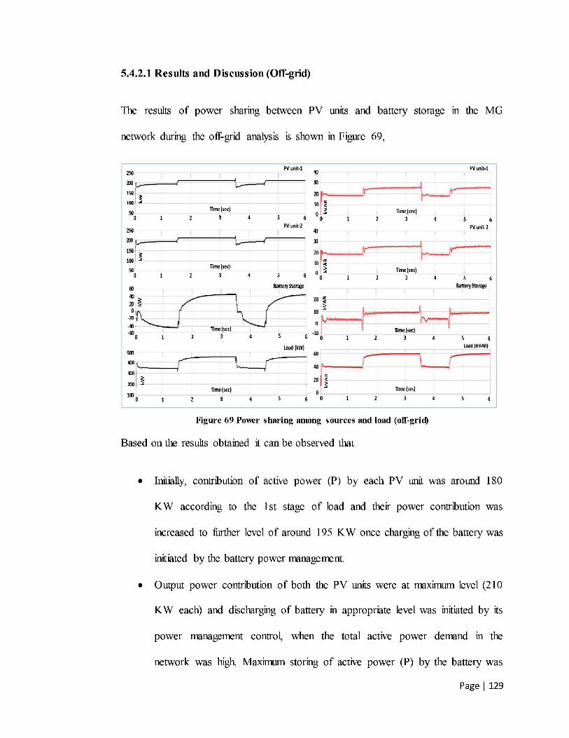
Page | 129
5.4.2.1 Results and Discussion (Off - grid)
The results of power sharing between PV units and battery storage in the MG
network during the off - grid analysis is shown in Figure 69 ,
Figure 69 Power sharing among sou rces and load (off - grid)
Based on the results obtained it can be observed that
Initially, contribution of active power (P) by each PV unit was around 180
KW according to the 1st stage of load and their power contribution was
increased to further level of around 195 KW once charging of the battery was
initiated by the battery power management.
Output power contribution of both the PV units were at maximum level (210
KW each) and discharging of battery in appropriate level was initiated by its
power managem ent control, when the total active power demand in the
network was high. Maximum storing of active power (P) by the battery was

Page | 130
found to be 45 KW and the maximum contribution was around 42 KW
respectively, when the total active power demand was low and hig h in MG
network.
Contribution of reactive power from each PV unit was 18 KVAR and 25
KVAR respectively during the low and high reactive power demand in the
MG network. Also the battery reactive power management control allowed
the battery to discharge arou nd 3 KVAR and 9 KVAR respectively during the
low and high reactive power demand in MG network.
Variation in reactive power level from each PV unit was observed around 5
KVAR (13 to 18 KVAR ) during the second stage of load varying condition.
Power variati on from the battery side was observed as more than 5 KVAR
during the load varying conditions in all three stages.
The voltage and frequency level in the MG network during off - grid analysis is
shown in Figure 70 and Table 22 .
Figure 70 Voltage and frequency level (off - grid)

Page | 131
Variation in frequency and voltage level was observed while changing of load in all
three stages. Variation in frequency level at first, second, and third stage of load
variation was observed around 50.1 to 49.75 Hz, 50.1 to 50.4 Hz, and 50 to 49.6 Hz
respectively. Similarly, voltage variation during first and third stage of load variation
was observed around 10% to -15% (with respect to 400V), and at second stage was
around 0 to 30% voltage (with respect to 400V) respectively.
Table 22 frequency and voltage level (off-grid)
Conditions
Frequency level (Hz) Variation (Hz)
w.r.t (50 Hz)
Voltage level (V) Variation (% )
w.r.t (400 V) Min Max Min Max
Load change (1st stage)
49.75 50.01 -0.25 to 0.01 340 440 15 % to 10 %
Load change (2nd stage)
50.1 50.4 0.1 to 0.4 400 520 0 % to 30 %
Load change (3rd stage) 49.6 50.0 -0.4 to 0 340 440 -15 % to 10 %
w.r.t (50 Hz) = with respect to nominal frequency; w.r.t (400 V) = with respect to nominal voltage
Thus from the results (Table 22), it can be concluded that the maximum and
minimum value of voltage/frequency level was found high and exceeding the
acceptable operating range of frequency and voltage level as per the Australian
network (NEM) and AS 60038 standard respectively.
5.4.2.2 Minimum SOC level (Off-grid)
As per the SOC control logics in power management, behavior of the MG power
system in particular during the off-grid mode of operation was analyzed when the
SOC of battery reaches equal/below 30% level. In addition, control behavior of the
load management was analyzed in order to ensure reliability of the system and safe
operation of the PV inverters while the MG was operating in off-grid mode.

Page | 132
When the SOC limit reaches a minimum level of 30% or below ( Figure 71 ),
SOC control of battery stops the battery from discharging.
LV feeder - 1 loads were switched off by the load management control when
total power demand was high i.e. above 380 KW , which exceeds 90%
nominal power (190 KW ) of each PV unit.
Once the feeder - 1 loa ds were switched off, the power contribution from each
PV unit was decreased from 210 KW to 195 KW according to the new load
condition. This was done to ensure safe operation of both PV units without
overloading it and also to improve reliability of the MG power system.
Figure 71 SOC and load management control at minimum SOC level

Page | 133
From the off-grid mode analysis, it was clear that an effective power sharing among
the PV units and better regulation of voltage and frequency level in the MG network
were ensured by means of implemented modified droop with virtual impedance
control in the PV inverters. Based on the SOC safe operating range of battery, power
management control strategy allows the battery to charge and discharge according to
the total demand and PV generation in the MG network. In addition, the power
management control also includes load management which initiates to switch-off
non-essential loads in case of the minimum SOC level of battery and deficit of
generation during excessive peak load, thereby ensuring power balance in the
network. Also, Dan Wu et al showed that SOC of the battery unit can be maintained
within the safe operating limits through the active power control strategy of power
management in the islanded MG network by automatically adjusting generation of
power from PV units and load consumption [45].
As compared to the on-grid analysis, voltage and frequency variation was high and
exceeds the standard limit in the off-grid analysis of MG network. This was due to
the lack of power inertia availability in the islanded MG network and also due to the
influence of PI based controller performance during transient conditions in the MG
network [18, 65].
5.4.3 On-grid to Off-grid transition mode Analysis
Because of using Grid-support Grid-form (GsGfm) VSI for the PV units and battery
storage, a smooth transition was ensured during the on-grid to off grid mode. In this
section, power variation/sharing among PV units and battery, variation in voltage

Page | 134
and frequency level were analyzed at that time of transition from the on - grid to of f
grid mode.
Transition (on - grid to off - grid) : At 2 sec, breaker was opened at the PCC
and MG was in transition from on - grid to off - grid mode.
5.4.3.1 Results and d iscussion (On - grid to Off - grid)
Results from this analysis as shown in Figure 72 , includes an active (P) and reactive
(Q) power sharing among sources/load along with voltage and fre quency level in the
MG network.
Figure 72 Power and voltage/frequency level during transition (on - grid to off - grid)

Page | 135
Before the transition mode, each PV unit power contribution was around 210
KW/5 KVAR and the battery discharge was around 27 KW/0 KVAR. At the
same time, total power demand in MG network was around 445 KW/45
KVAR and power import from the grid side was around 5 KW/ 30 KVAR.
During transition (2 sec), both PV units and battery storage continued to
operate in smooth manner with no variation in the power level was observed
from both the PV units and battery storage.
Due to the opening of breaker at PCC and loss of power support from the grid
side, contribution of power from both the PV units and battery storage were
as follows; each PV unit active power contribution was same (210 KW) and
reactive power contribution increased from 9 KVAR to 20 KVAR. Similarly,
active power contribution from the battery was increased from 27 KW to 32
KW and the reactive power increased from 0 KVAR to 10 KVAR.
Table 23 frequency and voltage level (on-grid to off-grid)
Condition
Frequency level (Hz) Variation (Hz)
w.r.t (50 Hz)
Voltage level (V) Variation (% )
w.r.t (400 V) Min Max Min Max
Transition 50.0 50.2 -0 to 0.2 392 412 -2 % to 3 %
w.r.t (50 Hz) = with respect to nominal frequency; w.r.t (400 V) = with respect to nominal voltage
As shown in the Figure 72 and Table 23, a small change in the frequency level was
observed from 50 to 50.20 Hz and a small variation in the voltage level was observed
from -2% to 3% (with respect to 400 V). This voltage and frequency level was
within the acceptable operating range of the Australian network and AS 60038
standard. However, this voltage and frequency level was small as compared to the

Page | 136
variation leve l during the varying load condition in the off - grid mode.
5.4.4 Total Harmonic Distortion (THD) (Results and discussion)
In this study, current and voltage THD level was analyzed in common bus of the
MG network and the obtained harmonics level was compare d to the AS / NZS
61000.2.2 and AS4777 standard level respectively . As per the AS 4777 standard ,
maximum limit of current harmonics (up to 50th order) injection from inte grated PV
inverter should be less than 5 % [110] and as per the AS / NZS 61000.2.2 standard,
compatibility level of voltage THD in the LV network should be less than 8% [111] .
(a) (b)
Figure 73 (a) Voltage THD; (b) Current THD
The voltage THD and current THD was found to be 0.48% and 3.93% respectively
in the common bus of MG network ( Figure 73 a and Figure 73 b). Thus from the
results obtained, it can be concluded that th e voltage and current THD level was
found to be minimum and within the tolerance level as per the AS / NZS 61000.2.2
and AS4777 s tandard respectively.

Page | 137
5.5 Conclusion
The unique feature of this developed model is the use of GsGfm type VSI which is
suitable for MG operation in the on-grid, off-grid and on-grid to off-grid transition
mode as compared to the grid-feeding or grid-forming type which can operate only
in the on-grid or off-grid mode.
Based on the analysis, following can be concluded:
The effectiveness of using the GsGfm type VSI in the MG network reflected
in the results where no power variation was observed ensuring smooth
operation of the MG during the on-grid to off-grid transition mode with the
varying load condition.
Use of the power management and modified power sharing control facility
ensured better power balance and voltage/frequency regulation in the MG
network in all three modes. Voltage and current THD level were found to be
within the AS4777 standard limit in the MG network.
Variations in the reactive power was particularly high as well as the variation
in voltage and frequency level exceeded the standard limit during the
transient conditions (varying load and varying solar irradiance) in the off-grid
mode than the on-grid mode of the MG network. This excessive variation
level of frequency and voltage can be due to the lack of inertia in the islanded
MG network and use of the under-performing PI based controller for GsGfm
type VSI during the transient conditions.

Page | 138
CHAPTER 6
Intelligent Control Strategy
6.1 Introduction
It was identified from the Chapter 5 results that variation in the power, frequency and
voltage was prominent in the off grid mode during the transient conditions. The
reason was due to the lack of inertia in the off-grid mode and under performance of
the PI based controller of the GsGfm type VSI in the PV and battery unit of the
developed MG model during the transient conditions. This problem could be solved
by implementing the optimization technique to tune control gains of the GsGfm type
VSI and achieve improvement in PQ factors of the islanded MG model.
Among the optimization techniques, PSO algorithm with the proposed cost function
was chosen in this research due to its benefits mentioned in the Section 2.8.1. The
main novelty of this work is the use of PSO algorithm with the proposed cost
function in the GsGfm type VSI of the DG units in the islanded MG model to
minimize the variation in power and frequency level (to be maintained within the
standard limit). The findings will indicate the efficiency of PSO algorithm with the
proposed cost function to obtain improved performance of the system through
minimization of power and frequency variation during the transient conditions in the
islanded MG network.
This chapter is organized as follows; Section 6.2 describes the method of
optimization including the formulation of cost function and setting parameters of

Page | 139
PSO algo rithm , S ection 6.3 demonst rates the optimization analysis and results
discussion incudes the power flow, power optimization and minimization of
frequency level in MG network , and S ection 6.4 gives the conc lusion of optimization
analysis.
6.2 Method of opti mization
In this study, control gains of the PI based voltage controllers of the previously
develo ped islanded MG model (Figure 52 ) was tuned through the PSO approach to
get optimised active (P) and reactive (Q) power flow from each DG unit through
regulat ing d - q axis reference current components (idref and iqref) of the inverter. In
addition, variation in frequency level was minimized during the load change
condition by applying penalty function in the cost function of PSO algorithm. A
single line diagram of MG model with application of PSO i s shown Figure 74 .
Figure 74 Single line diagram of the MG with the PSO application
For the proposed intelligent control strategy, PSO algorithm with the assigned cost
function was implemented through MATLAB - M - file programme in MATLAB -
SIMULINK software environment. PSO algorithm process was executed through
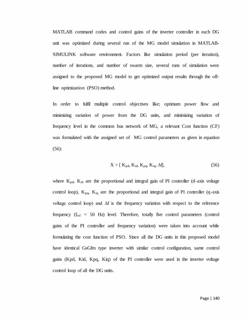
Page | 140
MATLAB command codes and control gains of the inverter controller in each DG
unit was optimized during several run of the MG model simulation in MATLAB-
SIMULINK software environment. Factors like simulation period (per iteration),
number of iterations, and number of swarm size, several runs of simulation were
assigned to the proposed MG model to get optimized output results through the off-
line optimization (PSO) method.
In order to fulfil multiple control objectives like; optimum power flow and
minimizing variation of power from the DG units, and minimizing variation of
frequency level in the common bus network of MG, a relevant Cost function (CF)
was formulated with the assigned set of MG control parameters as given in equation
(56):
X = [ Kpd, Kid, Kpq, Kiq, ∆f], (56)
where Kpd, Kid are the proportional and integral gain of PI controller (d-axis voltage
control loop), Kpq, Kiq are the proportional and integral gain of PI controller (q-axis
voltage control loop) and ∆f is the frequency variation with respect to the reference
frequency (fref = 50 Hz) level. Therefore, totally five control parameters (control
gains of the PI controller and frequency variation) were taken into account while
formulating the cost function of PSO. Since all the DG units in this proposed model
have identical GsGfm type inverter with similar control configuration, same control
gains (Kpd, Kid, Kpq, Kiq) of the PI controller were used in the inverter voltage
control loop of all the DG units.

Page | 141
6.2.1 Formulation of the cost function
The proposed cost function shown in the equation (57) below consists of Integral
Square Error (ISE) and penalty function:
Cost function (C) = ∫
+ XJ * YJ (57)
First term (ISE) in equation (57) is for optimizing the error level of (DG inverter)
voltage controller (by tuning PI controllers of the VSI voltage control loop through
PSO approach). In the equation above, e2 (t) is the error (in square) of control
variables with respect to time.
As per equation (58), combined error signal (e) is the summation of both voltage
error signals (Ea, Eb).
e = (Ea + Eb), (58)
Ea = (Vref (M) – Vd), (59)
Eb = (Vo – Vq), (60)
Vo = id*RD, (61)
Vref (M) = (E** - Vo), (62)
Id-ref =
Ea, (63)
Iq-ref =
Eb. (64)

Page | 142
As per the voltage control loop equations (59) and (60), by means of optimizing
voltage error signals (Ea, Eb), output reference currents (id-ref, iq-ref) can be regulated.
Regulating output reference currents (id-ref, iq-ref) of the voltage control loop will result
in the optimized power (active (P) and reactive (Q) power) flow from the DG
inverter.
Optimization of the voltage error signals (Ea, Eb) at input of the inverter voltage
control loop has been formulated in the ISE function by means of PSO tuning
approach for proportional (kp) and integral (ki) gains of the PI controllers, used in the
voltage control loop. As per equation (59), error signal Ea is the difference between
modified voltage reference signal and d-axis voltage component (Vd) of the inverter.
Equation (60) shows the expression of error signal Eb, which is the difference
between voltage drop (Vo) across virtual impedance and q-axis voltage component
(Vq) of the inverter. Voltage drop across virtual impedance is due to the effect of
inverter output current (id) over the virtual impedance (RD), shown in equation (61).
As per equation (62), modified voltage reference (Vref(M)) signal is the new voltage
reference signal, which is generated after extraction of the virtual impedance voltage
drop from the original voltage reference (E**) signal of droop controller.
By means of regulating the input voltage error signals (Ea and Eb), PI controllers in
the inverter voltage control loop generates the regulated output reference current
signals (id-ref, iq-ref)), expressed in equation (63) and (64) respectively:
Second term (penalty function) is considered for solving the problem constraint like
variation in frequency (∆f) level. Inequality constraint like frequency variation (∆f)

Page | 143
is added into the cost function by means of penalty function method. In general,
penalty factor is considered in the range from 100 to 10000 and constraint violation
index can be considered as 1, if violated otherwise it is 0 if not violated [101, 102,
123]. Second term of penalty function ( ) in cost function, constitutes penalty
factor (X) and constraint violation index ( . Constraint index j is considered for
frequency variation.
In this study, value of penalty constant ( ) was considered around 1000 and
constraint violation ( index for the frequency variation (∆f) was considered as 1, if
constraint (j) is violated otherwise it is 0 if not violated. Problem constraint of
frequency variation/deviations can be expressed as per the equation (65), and
equation (66) and (67) represents the control limit for frequency variation which was
considered around +/- 0.15 Hz (difference between measured frequency with respect
to the nominal frequency (50 Hz)).
∆f = (fref – f), (65)
( = 1; if | | > 0.15, (66)
( = 0; if | | < 0.15, (67)
where ∆f is the frequency variation which is to be maintained within 0.15 Hz as per
the Australian network standard (Table 8, in Section 4.3.1 of Chapter 4), fref is the
nominal frequency (50 Hz) and f is the measured frequency respectively.
Proposed PSO control algorithm, applied to the inverter control system of the MG
network is shown in Figure 75.

Page | 144
Figur e 75 Implementation of PSO control algorithm
6.2.2 MATLAB M - file codes with Process steps of PSO
Codes of MATLAB - m file has been developed with defined objective function for
optimization through off - line method of PSO process (Ta ble 24 ).
Table 24 MATLAB - m file codes for execution
Optim (m) file for the proposed objective function
% fitness (cost) function
function (E) = optim (PI) % Total error E, Inputs (PI)
% global variables
Global Ea Eb Ef % Ea e rror signal of Vd control loop
% Eb error signal of Vq control loop
% Ef error signal of frequency
PI = [0 PI]; % PI values
assignin („base , „PI , PI) % Assignin function
sim “ Microgrid_offgrid” % Start Simulink model simulation
E = (Ea *Ea + Eb *Eb); % square error (sum)
L = Length (Ef); % Ef in total length of simulation
Ef = Ef (round (L/2):end); % Ef during the transient condition

Page | 145
Constraint (ef) = Ef (abs (Ef) > 0.15) % check margin of frequency level
end
if empty (E) || ~ is empty (ef) || % Check size of (E) and (ef)
E = E + 1000; % add penalty
End
From the above codes, inverter voltage loop controller (Vd, Vq control loops) error
minimization through PSO algorithm has been considered with application of ISE
fitness function and additionally, frequency error (variation) has been optimized
during the total length (L) of model simulation time, and during the transient time
(L/2-length of time where the load changes) by means of applying penalty function
method. Implementation of Penalty function in the main cost function can ensure the
control of frequency variation level as per the assigned control limit (+/- 0.15 Hz
with reference to nominal level of 50 Hz) during the load change condition.
Details of process steps for the proposed PSO algorithm is shown in Table 25.
Table 25 Process steps of proposed PSO algorithm
PSO Process Steps
Step 1: Input the system parameters
Input the voltage errors (Ea, Eb), network frequency error (Ef) level
Assign upper and lower bounds for the control gains (Kp, Ki) of PI controllers
Set control limits for the frequency constraint,
Set ISE term function for optimizing problems of the PI controllers
Feed penalty function for the frequency constraint
Set other PSO parameters (Swarm size, iterations, C1/C2, r1/r2, initial velocity (V),
weight (w), etc.)

Page | 146
Step 2: Initialization
Initialize particle position and velocity randomly according to the upper and lower
bounds of control variables.
Evaluate objective function of the each particle in the initial population
Step 3: Set iterations K = K+1
Update inertia weight as per equation (28) - (Section 2.8.1.1 of Chapter2)
Step 4: Update velocity of particles
Update Velocity of each particle as per equation (31) - (Section 2.8.1.1 of Chapter2)
Step: 5 Update position of particles
Update Position of each particle as per equation (32) - (Section 2.8.1.1 of Chapter2)
Step 6: Update Indidual best (Pbest)
Evaluate fitness function of each particle with the current position and updates as
local best (Pbest)
Step 7: Update global best (Gbest)
Evaluate minimum value among the Pbest and update as global best
Step 8: If Iterations maximum iterations ; (go to Step 9, else to Step 3)
Step 9: Optimized output results : Gbest
Step 10: End
6.2.3 Settings of PSO parameters
Main parameters of PSO algorithm such as; particle size (number of swarms),
maximum iterations (number of iterations), lower and upper bounds of control
variables (Kp, ki), and control limit for ∆f were assigned during the process of
optimization, as given in Table 26.

Page | 147
Table 26 Main parameters of PSO
Parameters Value
Swarm size (n) 50
Number of iterations (i) 70
Lower bounds of control parameter (KP) for Vd and Vq control loop [ 0.001 0.001]
Lower bounds of control parameter (Ki) for Vd and Vq control loop [-1 -1]
Upper bounds of control parameter (KP) for Vd and Vq control loop [200 200]
Upper bounds of control parameter (Ki) for Vd and Vq control loop [100 100]
Frequency variation ∆f limit +/- 0.15 Hz
In this study, initial runs were made with the swarm size lower than 50, expected
feasible solution of the global value was not obtained. Thus the swarm size was
increased and at 50, the feasible solution of global value was achieved. Iteration
value of 70 was chosen for the optimization process based on the convergence curve
output (shown in Figure 76) in which a minimum of until 63rd generations
(iterations) was required to run to get the convergence. Assigning the limited search
boundary for the control gains of PI controller can cause the failure of determining
the global optimal value during the PSO process, in case if the global optimum value
is in outside of the boundary level. Extended boundaries have more chance to find
global optimum results, however it needs more time for finding that optimum level.
So, in this study, with reference to actual KP, Ki values of the conventional PI
controller, extended level of search boundaries were chosen in such a way to get the
global optimum value accordingly. Frequency variation limit was selected as per the
allowable operating frequency level of Australian network standard.

Page | 148
6.3 Simulation, analysis and results discussion
Proposed control parameters of the MG model were optimized while considering
steady state and transient (change - in load) conditions of the MG network. A
Convergence curve of PSO algorith m which is shown in Figure 76 , represents the
evaluation of proposed cost function at maximum iterations. Optimized control
parameters as given in Table 27 were applied in the voltage controller of the DG
inverters, optimized power flow with minimization o f power variation from the DG
units were ensured while MG was operating in the off - grid mode with load change
conditions.
Table 27 Optimized control parameters of the inverter voltage controller
Optimized parameters of PI Controller KPKi
Voltage (Vd) loop controller (d - axis) 19.0569 71.2539
Voltage (Vq) loop controller (q - axis) 7.3126 1.3501
Figure 76 Convergence curve

Page | 149
6.3.1 Power flow optimization
For this analysis, MG network configuration with specification of MG elements was
same (Figure 52, Table 17, 18, and 19) as discussed in Section (5.2) of Chapter-5.
During this analysis, active (P) and reactive (Q) power flow from each DG unit was
analyzed at different stage of load changing conditions.
Variation of load in MG network was considered in each stage as follows:
(d) In the first stage, total load was increased from 340 KW/39KVAR to 450
KW/58KVAR (1.5 sec),
(e) Then in the second stage, total load was reduced back to 340 KW/39 KVAR
(3.0 sec), and
(f) Finally in the third stage, total load was increased back to 450 KW/58 KVAR
(4.5 sec). `
In this study of off-grid mode analysis, as per the main objective function of PSO
algorithm which is mentioned in the equation (59), optimization level of active (P)
and reactive (Q) power flow obtained from the DG units (PV1, PV2, and battery
storage) are shown in Figure 77 and Figure 78 respectively. As from the results of
power flow, it can be observed that during the low demand (340 KW/39 KVAR) in
MG network, power contribution from each PV unit was observed around 195
KW/20 KVAR and charging power of the battery was around 45 KW/0 KVAR.
Similarly, during the high demand (450 KW/58 KVAR), power contribution from
each PV unit was observed maximum of around 210 KW/26.5 KVAR and power
discharge from the battery was around 36 KW/6 KVAR.
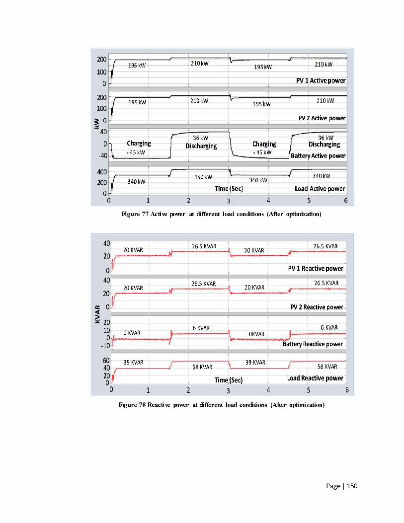
Page | 150
Figure 77 Active power at different load conditions (After optimization)
Figure 78 Reactive power at different load conditio ns (After optimization)

Page | 151
Figure 79 Current components (id, iq) of the DG inverters
PSO tuned PI controller in voltage control loop of the DG inverters which ensures
the regulation of inverter reference current components (id-ref, iq-ref) in d-q axis will
result in optimized d-axis current component (id) corresponding to the active power
(P) and q-axis current component (iq) related to the reactive power(Q). Inverter
current components (id, iq) of the PV units and battery storage is shown in Figure 79.
6.3.2 Active and Reactive power optimization
Optimization level of active power (P) flow from the DG units (PV1, PV2, and
battery storage) were analyzed and verified by comparing results before (Figure 80)
and after optimization (Figure 81). Similar comparison has been made for the
reactive power of the PV units and battery before (Figure 82) and after optimization
(Figure 83).
d-axis current component (id)
Battery inverter
PV inverters
q-axis current component (iq)
d-axis current component (id)
q-axis current component (iq) 0 1 2 3 4 5 6
Time (Sec)
1
0.50
- 0.5
- 1
0
0.5
1
- 0.5- 1
1
0.8
0.6
0.1
1.2
0
- 0.1- 0.2
per u
nit
per u
nit

Page | 152
Figure 80 Current components (id, iq) of the DG inverters
Figure 81 Active power of the PV units and battery storage (After optimization)
200
250
150
100
50
0
0
40
20
- 40
- 20
0 1 2 3 4 5 6
200 KW
180kW
from 1.35 sec
- 23 kW
210 kW
172 kW
At 3.06 sec
195 kW from 3.94 sec
210 kW
26 kW
- 24 kW At 3.21 sec
- 45 kW from 4.38 sec
24 kW At 5 sec
36 kW from 5.8 sec
Active power (PV units)
Active power (Battery)Time (Sec)
KW
195 kW from 0.9 sec
- 45 kW
At 2.1 sec
36 kW from 2.8 sec
from 2.3 sec from 5.3 sec
200
250
150
100
50
0
0
40
20
- 40
- 20
0 1 2 3 4 5 6
196.5 KW
195 kW from 0.2 sec
- 45 kW 0.24 sec
- 40 kW
210 kW
178 kW At 3.06 sec
195 kW
from 3.51 sec
210 kW
25 kW
At 1.62 sec
36 kW from 2.5 sec
- 40 kW At 3.2 sec
- 45 kW from 4.01 sec
27 kW At 4.6 sec
36 kW from 5.5 sec
Active power (PV units)
Active power (Battery)Time (Sec)
KW
from 2 sec
210 kW from 5 sec

Page | 153
Figure 82 Reactive power of PV units and battery storage (Before optimization)
Figure 83 Reactive power of PV units and battery storage (After optimization)
0
10
20
30
40
0
20
10
-10
20 kVAR from 0.3 sec
30 kVAR
20 kVAR
26.5 kVAR
Time (Sec)
KV
AR
0 1 2 3 4 5 6
Reactive power (PV units)
Reactive power (Battery)
26.5 KVAR
6 KVAR7 KVAR
11 KVAR
6 KVAR0 KVAR
0 KVARfrom 0.9 sec
30
22.5 kVAR
from 2.18 sec
11kVAR
At 0.12 sec
- 5 KVAR
12 KVAR21 KVAR
-6KVAR
6 KVARfrom 1.85 sec
0
10
20
30
40
0
20
10
-10
20 kVAR from 0.17 sec
28.5 30.5 kVAR
22 kVAR
31 kVAR
4 kVAR
At 0.1 sec4 kVAR
2
4 kVAR
20 kVAR
- 4 kVAR - 2 kVAR
4 kVAR
Time
KV
AR
0 1 2 3 4 5 6
Reactive power (PV units)
Reactive power (Battery)Time (Sec)
Reactive power (PV units)
Reactive power (Battery)
20 KVARfrom 0.17 sec
20 kVAR
At 0.1 sec4 kVAR
6 KVAR
26.5 KVAR
26.5 KVAR
6 KVAR
0 KVAR0 KVAR
20 kVAR
28 KVAR
19.5 KVARfrom 1.6 sec
0 KVARfrom 0.15 sec
9 kVAR 9 kVAR 9 kVAR
from 1.6 sec
- 3 kVAR

Page | 154
6.3.2.1 Performance of DG inverters control (at initial state)
Maximum overshoot in power level of the DG inverters, and time taken by the DG
inverters to reach their steady state power level were analyzed during the initial state
of simulation.
As per the Figure 80, Figure 81, and Table 28, it can be concluded that
maximum overshoot in active power level of the PV units for PSO based
inverter control (after optimization) was 1.5 KW more than the steady state
power value (0.76% higher) whereas for the PI based inverter control (before
optimization), it was 5 KW more than the steady state power value (2.5 %
higher). Also, PSO-based inverter control enables the inverter of PV units to
reach the steady state active power level in a significantly lower time as
compared to the PI-based inverter control.
Results from the Figure 82, Figure 83, and Table 28, clearly indicates no over
shoot in reactive power level after optimization for the PV units. However for
before optimization, the over shoot in power difference was 2.5 KVAR more
than the steady state value. In addition, the PV units reach steady state
reactive power level in less time after optimization.
Likewise, overshoot in reactive power level of the battery unit (difference
between the steady state value and the excessive power shoot) before and
after optimization were 4KVAR and 7KVAR respectively as shown in Figure
82, Figure 83, and Table 27. Also, battery unit reaches steady state reactive
power value faster after optimization during the initial state of simulation.

Page | 155
Table 28 Performance of the DG inverters (at initial state)
PV Units – Active Power overshoot and Steady state response
Load (KW)
Steady state value
PV Power (KW)
Overshoot in Active Power (KW)
Time (sec) to reach Steady state value
Before optimization
After optimization
Before optimization
After optimization
340 195 200 196.5 0.9 0.2
PV Units – Reactive Power overshoot and Steady state response
Load (KVA
R)
Steady state value
PV Power (KVAR)
Overshoot in Reactive Power (KVAR)
Time (sec) to reach Steady state value
Before optimization
After optimization
Before optimization
After optimization
39 20 22.5 20 0.3 0.17
Battery – Reactive Power overshoot and Steady state response
Load (KVA
R)
Steady state value
PV Power (KVAR)
Overshoot in Reactive Power (KVAR)
Time (sec) to reach Steady state value
Before optimization
After optimization
Before optimization
After optimization
39 0 7 4 0.9 0.15
6.3.2.2 Steady state response (Active power) of the DG inverters (At different
loads)
Steady state response in active power level before and after optimization of
the PV units and battery storage at different stage of load conditions in the
MG network is shown in Table 29. As shown in the Figure 80 and Figure 81,
during high (450 KW) and low demand (340 KW) condition in the MG
network, steady state active power level of the PV units was around 210 KW
and 195 KW respectively. Similarly, steady state discharging and charging
power level of battery was around 45 KW and 36 KW during high and low
demand conditions respectively. As shown in Table 29, PV units and battery
takes less time to reach the steady state active power level after optimization
during the different stage of load conditions.

Page | 156
Table 29 Steady state response (Active power) of DG inverters (at different loads)
PV Units – Steady state response of Active power
Simulation Time (sec)
Load (KW)
Steady state value PV Power (KW)
Time (sec) to reach Steady state value
Before optimization
After Optimizatio
n
1.5 to 3 450 210 0.8 0.5
3 to 4.5 340 195 0.94 0.51
4.5 to 6 450 210 0.8 0.5
Battery – Steady state response of Active power
Simulation Time (sec)
Load (KW)
Steady state value PV Power (KW)
Time (sec) to reach Steady state value
Before optimization
After Optimizatio
n
0 to 1.5 340 -45 1.35 0.24
1.5 to 3 450 36 1.3 1
3 to 4.5 340 -45 1.38 1.01
4.5 to 6 450 36 1.3 1
6.3.2.3 Steady state response (Reactive power) of DG inverters (at high demand)
Steady state response in reactive power level before and after optimization of the PV
units and battery storage during the high reactive power demand condition in MG
network is shown in Table 30.
As shown in Figure 82, Figure 83, and Table 30, reactive power contribution
from each PV unit was around 26.5 KVAR and from the battery was around
6 KVAR respectively during the high reactive power demand (58 KVAR) in
MG network. As per the results in Table 30, PV units and battery storage
reach steady state reactive power value faster after optimization during the
high demand (58 KVAR) condition of simulation time (1.5 to 3 sec).

Page | 157
Table 30 Steady state response (Reactive power) of DG inverters (high demand)
PV Units – Steady state response of Reactive Power
Simulation Time (sec)
Load (KVAR)
Steady state value PV Power (KVAR)
Time (sec) to reach Steady state value
Before optimization
After optimization
1.5 to 3 58 26.5 0.68 0.1
Battery – Steady state response of Reactive Power
Simulation Time (sec)
Load (KVAR)
Steady state value PV Power (KVAR)
Time (sec) to reach Steady state value
Before optimization
After optimization
1.5 to 3 38 6 0.35 0.1
6.3.2.4 Reactive power variation from DG units (during load change condition)
Variation in reactive power level during the time of load change condition for the PV
units and battery storage before and after optimization is shown in the Table 31.
Table 31 Reactive power variation (during load change conditions)
PV Units – Reactive power variation
Simulation Time (sec)
Change in Load
(KVAR)
Reactive Power (KVAR) variation (Max)
Reactive Power (KVAR) variation (Min)
Before optimization
After optimization
Before Optimizat
ion
After optimizatio
n
3 58 to 39 11 to 20 26.5 to 28 26.5 to 30 19.5 to 20
Battery – Reactive power variation
Simulation Time (sec)
Change in Load
(KVAR)
Reactive Power (KVAR) variation (Max)
Reactive Power (KVAR) variation (Min)
Before optimization
After optimization
Before optimizati
on
After optimizatio
n
1.5 39 to 58 12 to 6 9 to 6 0 to -3 -5 0 to -3
3 58 to 39 6 to 21 6 to 9 0 0
4.5 39 to 58 0 to 6 9 to 6 11 to 6 0
As shown in Figure 82, Figure 83, and Table 31, at the time (3 sec) of load
switch-off (from 58 KVAR to 39 KVAR) condition, that the reactive power
variation in maximum and minimum level (deviation from the steady state

Page | 158
reactive power value) for the PV units after optimization was 1.5 KVAR and
0.5 KVAR respectively whereas before optimization, it was 9 KVAR and 3.5
KVAR respectively. Significant reduction in the variation of reactive power
level was ensured after optimization.
As per Table 31, during the load change conditions at different simulation
time that the reactive power variation for the battery after optimization was
maximum of around 3 KVAR, whereas before optimization, for the battery,
the maximum reactive power variation was more than 5 KVAR in all the time
of load change conditions. Reactive power variation in the battery unit during
load change at various simulation times was higher before the optimization.
6.3.3 Minimization of frequency variation
The frequency level in common bus network of the MG power system was analyzed
during the load change conditions in each stage. During the simulation, details of
load with switching time were considered as below:
At 1.5 sec, load switch-on (340 KW/39 KVAR to 450 KW/58 KVAR)
At 3 sec, load switch-off (450 KW/58 KVAR to 340 KW/39 KVAR)
At 4.5 sec, load switch-on (340 KW/39 KVAR to 450 KW/58 KVAR)
Variation in frequency level with the before and after optimization in the islanded
MG network during the time of load change condition in each stage is shown in
Figure 84, Figure 85, and Table 32 respectively. Acceptable operating range of
frequency level as per the Australian network standard (NEM) [110, 117] was

Page | 159
compared with the frequency level before and after optimization is shown in Table
33.
Results from the Table 32, tabulated based on the values obtained from the Figure 84
and Figure 85 clearly shows that the frequency variation in the islanded MG network
was minimized after optimization. Maximum frequency level of 50.4 Hz observed
during the load switch off condition in the MG network without the PSO algorithm
was minimized into 50.07 Hz by implementing PSO algorithm. Similarly, Minimum
frequency level of 49.6 Hz observed during the load switch on condition in the MG
network without optimization was improved to 49.85 Hz by implementing PSO
algorithm.
Figure 84 Frequency variation during load change (Before optimization)
Figure 85 Frequency variation during load change (After optimization)
51.5
51.0
50.5
50.0
49.5
49.0
48.00 1 3 4 5 62
Time (Sec)
Hz
49.75 hz
50.4 hz
49.6 hz
50.15 hz50.0 hz
48.5
50.15 hz 50.1 hz
51.5
51.0
50.5
50.0
49.5
49.0
48.00 1 3 4 5 62
Time (Sec)
Hz
49.75 hz
50.4 hz
49.6 hz
50.15 hz50.0 hz 50.1 hz
48.5
50.15 hz50.07 hz
49.85 hz49.96 hz
49.94 hz 49.96 hz50.0 hz50.0 hz
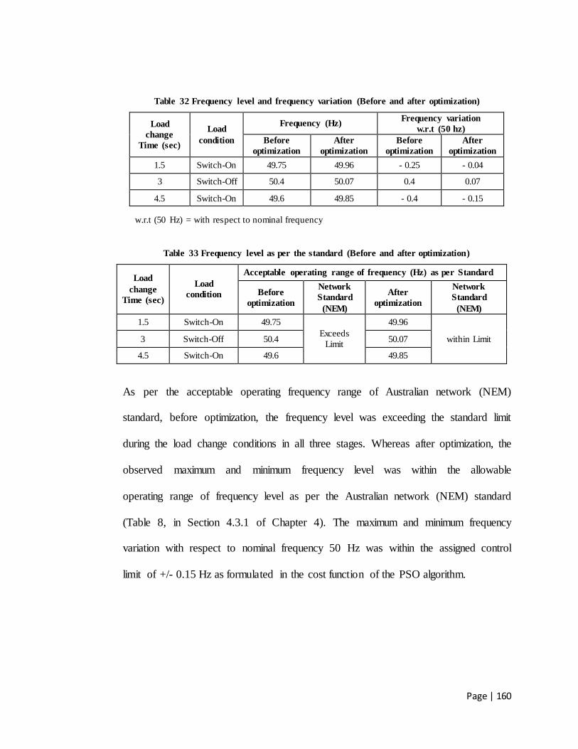
Page | 160
Table 32 Frequency level and frequency variation (Before and after optimization)
Load change
Time (sec)
Load condition
Frequency (Hz) Frequency variation w.r.t (50 hz)
Before optimization
After optimization
Before optimization
After optimization
1.5 Switch-On 49.75 49.96 - 0.25 - 0.04
3 Switch-Off 50.4 50.07 0.4 0.07
4.5 Switch-On 49.6 49.85 - 0.4 - 0.15
w.r.t (50 Hz) = with respect to nominal frequency
Table 33 Frequency level as per the standard (Before and after optimization)
Load change
Time (sec)
Load condition
Acceptable operating range of frequency (Hz) as per Standard
Before optimization
Network Standard
(NEM)
After optimization
Network Standard
(NEM)
1.5 Switch-On 49.75 Exceeds
Limit
49.96
within Limit 3 Switch-Off 50.4 50.07
4.5 Switch-On 49.6 49.85
As per the acceptable operating frequency range of Australian network (NEM)
standard, before optimization, the frequency level was exceeding the standard limit
during the load change conditions in all three stages. Whereas after optimization, the
observed maximum and minimum frequency level was within the allowable
operating range of frequency level as per the Australian network (NEM) standard
(Table 8, in Section 4.3.1 of Chapter 4). The maximum and minimum frequency
variation with respect to nominal frequency 50 Hz was within the assigned control
limit of +/- 0.15 Hz as formulated in the cost function of the PSO algorithm.
Page | 161
6.4 Discussion
It was found from the previous study in Chapter 5 that the power variation in the
DG units and frequency variation in MG network were high especially during the
transient condition in the off-grid/islanded mode of the simulated MG model in
MATLAB-SIMULINK software environment. Thus an optimization approach with
the help of a PSO based intelligent control strategy is made to reduce/minimize the
power and frequency variation in the MATLAB-SIMULINK MG model during the
transient condition in the off-grid mode. Simulation was also performed on the
islanded network of MG model with the PI control strategy. A comparison was made
between the results obtained from the MG model before and after optimization.
In this study, PSO algorithm along with the assigned cost function was implemented
in the islanded mode of the MG power system. The cost function was formulated
with two terms namely ISE fitness function and penalty function. ISE fitness
function was applied to optimize the control parameters of inverter voltage
controller, in order to get optimized power flow and minimization of power variation
from the DG units through regulating inverter d-q axis reference currents (id-ref, iq-ref).
Similarly, penalty function was formulated to solve the inequality constraint of
frequency variation as per assigned limit (+/- 0.15 Hz with reference to nominal
frequency 50 Hz) while changing the load condition in the MG network.
As per the results from Figure 80, Figure 81, Figure 82, Figure 83, and Table 28, PV
unit after optimization offers reduced or less overshoot in active power (with respect
to steady state active power value) and no overshoot in reactive power level (with
respect to steady state reactive active power value) during the initial state of

Page | 162
simulation time as compared to the results before optimization. Also, time taken to
reach the steady state active and reactive power value of the PV units was also faster
after the optimization during the initial state of simulation (Table 28) and different
stage of load conditions (Table 28, Table 29). Similarly as shown in Figure 82,
Figure 83 and results from the Table 29, battery storage showed superior
characteristics in terms of overshoot in reactive power level with respect to the
steady state reactive power value and time taken to reach the steady state
active/reactive power value after optimization during the initial state of simulation
and different stage of load conditions (Table 30).
As per the results from Table 31, maximum and minimum reactive power variation
(deviation with respect to steady state reactive power value) was also higher before
optimization for both the PV units and battery storage during the time of load change
conditions.
As per the results from Figure 84, Figure 85, and Table 32, due to the PSO algorithm
application in the islanded MG network, variation/deviation in frequency level with
respect to nominal frequency was minimum as compared to the variation in the MG
network with PI based control. During the load switch-off and switch-on condition,
the frequency variation was minimized to 0.04, 0.07 and 0.15 Hz respectively by
PSO algorithm application as compared to the variation of 0.25, 0.5 and 0.4 Hz with
PI controller.
The limitation in using such optimization algorithms to obtain the optimized results
that the process is time consuming where the number of iterations and parameters

Page | 163
chosen has to be in broad range so as to obtain convergence. Also the simulation has
to be extended to other test cases to assess the behavior and performance of the
system.
6.5 Conclusion
A comparison was made for the power/frequency variation between the conventional
PI inverter control (before implementing the optimization algorithm) and PSO tuned
PI inverter control (after the optimization) of the GsGfm type VSI for the DG units
in the islanded MG model.
Based on the results, it can be observed that
variation in the power/frequency was considerably lower for the islanded MG
power system after optimization compared to the results before the
optimization. DG units reached steady state faster with the minimal overshoot
value after implementing the PSO algorithm showing its efficiency.
penalty function incorporated into the PSO algorithm also ensured the
frequency variation to be within the acceptable operating range as per the
standard limit, thereby enhancing the system stability. This aspect makes this
work unique compared to the previous researchers work.
Use of the PSO algorithm with the proposed cost function apart from the
implemented co-ordinated power management and power sharing control strategies
adds additional benefit by minimizing the PQ issues like power variation and
frequency variation further in the GsGfm type VSI of the DG units in the islanded

Page | 164
MG system. This type of work had not been reported before as per the author‟s
knowledge.

Page | 165
CHAPTER 7
Conclusion and Future Work
This thesis addressed the effect of various scenarios on the PQ factors in a PV based
MG network through simulation and experimental approach. The main outcomes
from this research, contribution to the knowledge, novelty of the work and
recommendations for the future work are highlighted in this chapter.
7.1 Main outcomes
The main outcomes obtained from this thesis are summarized below:
In Chapter 3, multiple scenarios were introduced simultaneously in the PV
based MG network and it was found that each scenario had significant
influence on the PQ factors. Non-linear and composite loads affected the
current THD, VUF by peak demand as per the daily load profile and uneven
distribution of the single phase PV units & single phase loads followed by the
power flow variation and local voltage fluctuation due to the PV output
power variation (solar disturbance due to the cloud effect).
In Chapter 4, real cloud effect and other scenarios were introduced in a real-
time PV based MG network and its effect on the PQ factors have been
studied. Variation in the voltage/frequency level (particularly high in the off-
grid mode), VUF and neutral current level was found to increase with the
varying unbalanced load PV generation conditions. Also, overall THD and
Page | 166
individual odd-order current THD level was highly influenced by different
PV power levels caused by the real cloud effect.
In Chapter 5, better power balance and voltage/frequency regulation was
ensured in the PV based MG model implemented with the co-ordinated
power management and power sharing control in GsGfm type VSI of the DG
units in the MG network operated in on-grid, off-grid and on-grid to off-grid
transition mode. Among the PQ factors, THD level was within the standard
limit. However, variation in the reactive power, voltage and frequency was
prominent in the off-grid mode. Use of GsGfm type VSI ensured smooth
operation of the MG during the on-grid to off-grid transition mode under the
varying load condition.
In Chapter 6, variation in the power/frequency level was minimized further in
the islanded PV based MG model by implementing PSO algorithm with the
proposed cost function to tune control gains of the PI controller in the GsGfm
type VSI. Penalty function integrated into the PSO algorithm ensured
frequency variation with the acceptable operating range as per the standard
limit in the islanded MG model.
7.2 Contributions of the thesis
This thesis was mainly focused towards the following contributions in a PV based
MG network:
Most of the studies on PQ issues in the PV based MG network were mainly
focused on quantification of THD with few works on other PQ factors like

Page | 167
VUF, etc. Also the simulation or experiment was carried out using individual
or a combination of few scenarios. However, all these scenarios could
simultaneously affect the PQ factors in the MG network. Thus, in this
research, all the scenarios like varying solar irradiance (cloud effect), various
PV penetration levels, unbalanced PV generation and unbalanced load
conditions has been introduced into the MG network simultaneously and its
influence on the PQ factors have been highlighted through the simulation
(PSS SINCAL software) and experimental approach.
Based on the literature survey, it was found that either grid-feeding or grid-
forming type VSI was used for the DG units in the MG network. The major
disadvantage of using the former and latter is that it can be operated only in
either mode leading to the use of additional hardware for the mode transfer.
Thus, in this research, GsGfm type VSI was utilized which has the ability to
operate in both grid connected and island mode without the need for
changing the control configuration or additional hardware as in the case of
the former. It also ensured smooth operation of MG during the on-grid to off-
grid transition mode. Power management and power sharing control was also
implemented to achieve better power sharing among the DG sources, power
balance, coordinated operation between battery and PV units and regulation
of voltage and frequency level in the MG network during on-grid, off-grid,
and on-grid to off-grid of the MG operation.
Since the variation in power and frequency was found to be higher in the
islanded mode of the MG network implemented with the co-ordinated power
Page | 168
management/power sharing control strategies in the GsGfm type VSI of the
DG units in the islanded MG network, a PSO algorithm with proposed cost
function was applied to minimize the variation effectively. Penalty function
was also incorporated into the algorithm to maintain the frequency within the
acceptable operating range as per the standard limit. Optimizing the PQ
factors using PSO algorithm with the proposed cost function in the islanded
PV based MG network with GsGfm type VSI was the main contribution and
novelty of this thesis.
7.3 Future works
The future research work will involve the fulfillment of following objectives in a PV
based MG network as follows:
Development of advanced optimization hybrid control algorithm for
minimizing the voltage variation level (as per the standard operating range) in
the islanded MG network during the transient conditions.
To further minimize harmonics level in the MG network by means of
implementing advanced optimized control algorithm for inverter control of
the DG units.
In order to improve the stability and dynamic response of the MG control
system during the transient conditions, a robust control strategy with
optimized control technique will be developed and implemented for the MG
control system.

Page | 169
Novel control technique will be developed for the PQ devices to mitigate the
unbalance voltage level due to the effect of uneven distribution of single
phase loads and uneven impedance level in the distribution network of MG
power system.
Using optimized multi-objective control algorithm, economic energy
management will be developed for the PV based MG power system to ensure
reduced energy cost and minimization of the power loss in MG network.

Page | 170
References
[1] D. Henry and J. E. Ramirez‐Marquez, "On the Impacts of Power Outages during
Hurricane Sandy—A Resilience‐Based Analysis," Systems Engineering, vol. 19, pp. 59-75, 2016.
[2] S. Communities, "Building our nation’s resilien e to natural disasters." [3] A. Kwasinski, J. Eidinger, A. Tang, and C. Tudo-Bornarel, "Performance of electric
power systems in the 2010-2011 christchurch, new zealand, earthquake sequence," Earthquake Spectra, vol. 30, pp. 205-230, 2014.
[4] P. A. Adam Wilson. (December 2016). "Microgrid Deployment Tracker: Research
Report (4Q2016)". [Available Online]: https://www.navigantresearch.com/research/microgrid-deployment-tracker-4q16 Access Date: 10th January 2017.
[5] N. Hatziargyriou, Microgrids: architectures and control: John Wiley & Sons, 2013. [6] S. Chowdhury and P. Crossley, Microgrids and active distribution networks: The
Institution of Engineering and Technology, 2009. [7] H. Liang and W. Zhuang, "Stochastic modeling and optimization in a microgrid: A
survey," Energies, vol. 7, pp. 2027-2050, 2014. [8] I. I. E. Commission, "Microgrids for disaster preparedness and recovery-With
electricity continuity plans and systems," White paper, Geneva, Switzerland, 2014. [9] N. Zhou, "International Microgrid Assessment: Governance, INcentives, and
Experience," 2014. [10] M. Stadler, G. Cardoso, S. Mashayekh, T. Forget, N. DeForest, A. Agarwal , et al.,
"Value Streams in Microgrids: A literature," 2015. [11] L. Bird, M. Milligan, and D. Lew, "Integrating variable renewable energy: Challenges
and solutions," National Renewable Energy Laboratory, 2013. [12] K. A. Nigim and W.-J. Lee, "Micro grid integration opportunities and challenges," in
Power Engineering Society General Meeting, 2007. IEEE, 2007, pp. 1-6. [13] S. Voima and K. Kauhaniemi, "Technical Challenges of Smart-and Microgrids," in
Renewable Efficient Energy II Conference, Vaasa, Finland , 2012, pp. 21-22. [14] T. D. C. Huayllas, D. Ramos, and R. Vasquez-Arnez, "Microgrid systems: Current
status and challenges," in Transmission and Distribution Conference and Exposition: Latin America (T&D-LA), 2010 IEEE/PES, 2010, pp. 7-12.

Page | 171
[15] A. Salam, A. Mohamed, and M. Hannan, "Technical challenges on microgrids,"
ARPN Journal of engineering and applied sciences, vol. 3, pp. 64-69, 2008. [16] O. Palizban, K. Kauhaniemi, and J. M. Guerrero, "Microgrids in active network
management–part II: System operation, power quality and protection," Renewable and Sustainable Energy Reviews, vol. 36, pp. 440-451, 2014.
[17] P. Basak, S. Chowdhury, S. H. nee Dey, and S. Chowdhury, "A literature review on
integration of distributed energy resources in the perspective of control, protection and stability of microgrid," Renewable and Sustainable Energy Reviews, vol. 16, pp. 5545-5556, 2012.
[18] D. E. Olivares, A. Mehrizi-Sani, A. H. Etemadi, C. A. Cañizares, R. Iravani, M.
Kazerani, et al., "Trends in microgrid control," IEEE Transactions on smart grid, vol. 5, pp. 1905-1919, 2014.
[19] A. B. Baggini, Handbook of power quality: Wiley Online Library, 2008. [20] H. Mahmood, D. Michaelson, and J. Jiang, "Accurate reactive power sharing in an
islanded microgrid using adaptive virtual impedances," IEEE Transactions on Power Electronics, vol. 30, pp. 1605-1617, 2015.
[21] Y. Xu, W. Zhang, G. Hug, S. Kar, and Z. Li, "Cooperative control of distributed energy
storage systems in a microgrid," IEEE Transactions on Smart Grid, vol. 6, pp. 238-248, 2015.
[22] M. S. Mahmoud, M. S. U. Rahman, and M.-S. Fouad, "Review of microgrid
architectures–a system of systems perspective," IET Renewable Power Generation, vol. 9, pp. 1064-1078, 2015.
[23] O. Dag and B. Mirafzal, "On stability of islanded low-inertia microgrids," in 2016
Clemson University Power Systems Conference (PSC) , 2016, pp. 1-7. [24] D. W. Gao, Energy Storage for Sustainable Microgrid: Academic Press, 2015. [25] W. El-Khattam and M. Salama, "Distributed generation technologies, definitions
and benefits," Electric power systems research, vol. 71, pp. 119-128, 2004. [26] G. Pepermans, J. Driesen, D. Haeseldon kx, R. Belmans, and W. D’haeseleer,
"Distributed generation: definition, benefits and issues," Energy policy, vol. 33, pp. 787-798, 2005.
[27] M. H. Bollen and F. Hassan, Integration of distributed generation in the power
system vol. 80: John wiley & sons, 2011.

Page | 172
[28] N. Rugthaicharoencheep and S. Auchariyamet, "Technical and Economic Impacts of distributed generation on distribution system," World Academy of Science, Engineering and Technology, vol. 64, 2012.
[29] Z. Shuai, Y. Sun, Z. J. Shen, W. Tian, C. Tu, Y. Li , et al., "Microgrid stability:
Classification and a review," Renewable and Sustainable Energy Reviews, vol. 58, pp. 167-179, 2016.
[30] Q. Fu, A. Nasiri, A. Solanki, A. Bani-Ahmed, L. Weber, and V. Bhavaraju, "Microgrids:
Architectures, Controls, Protection, and Demonstration," Electric Power Components and Systems, vol. 43, pp. 1453-1465, 2015.
[31] G. Buigues, A. Dyśko, V. Valverde, I. Zamora, and E. Fernández, "Mi rogrid
Protection: Technical challenges and existing techniques," in International Conference on Renewable Energies and Power Quality (ICREPQ’13) , 2013.
[32] E. M. Sandhu and D. T. Thakur, "Issues, Challenges, Causes, Impacts and Utilization
of Renewable Energy Sources-Grid Integration," Int. Journal of Engineering Research and Applications, vol. 4, pp. 637-643, 2014.
[33] R. Bayindir, E. Hossain, E. Kabalci, and R. Perez, "A comprehensive study on
microgrid technology," International Journal of Renewable Energy Research, vol. 4, pp. 1094-1107, 2014.
[34] C. Bhende and A. Kalam, "Power quality conditioner for microgrid," in Power
Engineering Conference (AUPEC), 2013 Australasian Universities, 2013, pp. 1-4. [35] M. Begovic, J. Zhang, D. Novosel, and N. Cho, "Harmonic Distortion in Microgrids
and Distribution Systems with Photovoltaic Generators," in System Sciences (HICSS), 2015 48th Hawaii International Conference on, 2015, pp. 2586-2594.
[36] R. Torquato, F. C. Trindade, and W. Freitas, "Analysis of the harmonic distortion
impact of photovoltaic generation in Brazilian residential networks," in 2014 16th International Conference on Harmonics and Quality of Power (ICHQP) , 2014, pp. 239-243.
[37] Z. Liu, X. Xu, H. A. Abdelsalam, and E. Makram, "Power System Harmonics Study for
Unbalanced Microgrid System with PV Sources and Nonlinear Loads," Journal of Power and Energy Engineering, vol. 3, p. 43, 2015.
[38] H. Qian, J. Zhang, J.-S. Lai, and W. Yu, "A high-efficiency grid-tie battery energy
storage system," IEEE transactions on power electronics, vol. 26, pp. 886-896, 2011. [39] V. Barbu, G. Chicco, F. Corona, N. Golovanov, and F. Spertino, "Impact of a
photovoltaic plant connected to the MV network on harmonic distortion: an experimental assessment," Scientific Bulletin of Universitatea Politehnica din Bucuresti (UPB), Series C, vol. 75, pp. 179-193, 2013.

Page | 173
[40] P. Trichakis, P. Taylor, L. M. Cipcigan, P. Lyons, R. Hair, and T. Ma, "An investigation of voltage unbalance in low voltage distribution networks with high levels of SSEG," in Universities Power Engineering Conference, 2006. UPEC'06. Proceedings of the 41st International, 2006, pp. 182-186.
[41] A. Nagarajan, Model Development and Analysis of Distribution Feeders with High
Penetration of PV Generation Resources: Arizona State University, 2015. [42] C. Y. Lau, C. K. Gan, C. H. Tie, K. A. Baharin, and M. F. Sulaima, "Passing-Cloud
Effects of Solar Photovoltaic System on Distribution Network Voltages," in Applied Mechanics and Materials, 2015, pp. 551-555.
[43] A. Woyte, V. Van Thong, R. Belmans, and J. Nijs, "Voltage fluctuations on
distribution level introduced by photovoltaic systems," IEEE Transactions on energy conversion, vol. 21, pp. 202-209, 2006.
[44] M. Datta, T. Senjyu, A. Yona, T. Funabashi, and C.-H. Kim, "A frequency-control
approach by photovoltaic generator in a PV–diesel hybrid power system," IEEE Transactions on Energy Conversion, vol. 26, pp. 559-571, 2011.
[45] D. Wu, F. Tang, T. Dragicevic, J. C. Vasquez, and J. M. Guerrero, "Autonomous active
power control for islanded ac microgrids with photovoltaic generation and energy storage system," IEEE Transactions on Energy Conversion, vol. 29, pp. 882-892, 2014.
[46] H. Mahmood, D. Michaelson, and J. Jiang, "Decentralized Power Management of a
PV/Battery Hybrid Unit in a Droop-Controlled Islanded Microgrid," IEEE Transactions on Power Electronics, vol. 30, pp. 7215-7229, 2015.
[47] L. Freris and D. Infield, Renewable energy in power systems: John Wiley & Sons,
2008. [48] S. Chakraborty, M. G. Simões, and W. E. Kramer, "Power electronics for renewable
and distributed energy systems," A Sourcebook of Topologies, Control and Integration, pp. 235-265, 2013.
[49] G. N. Tiwari and R. K. Mishra, Advanced renewable energy sources: Royal Society of
Chemistry, 2012. [50] H. Häberlin, Photovoltaics system design and practice: John Wiley & Sons, 2012. [51] R. Kotti and W. Shireen, "Efficient MPPT control for PV systems adaptive to fast
changing irradiation and partial shading conditions," Solar Energy, vol. 114, pp. 397-407, 2015.
[52] X. Tan, Q. Li, and H. Wang, "Advances and trends of energy storage technology in
microgrid," International Journal of Electrical Power & Energy Systems, vol. 44, pp. 179-191, 2013.

Page | 174
[53] F. S. Barnes and J. G. Levine, Large energy storage systems handbook: CRC press,
2011. [54] R. Carnegie, D. Gotham, D. Nderitu, and P. V. Preckel, "Utility scale energy storage
systems," State Utility Forecasting Group, Purdue University, West Lafayette, 2013. [55] A. Chatzivasileiadi, E. Ampatzi, and I. Knight, "Characteristics of electrical energy
storage technologies and their applications in buildings," Renewable and Sustainable Energy Reviews, vol. 25, pp. 814-830, 2013.
[56] M. Vilathgamuwa, D. Nayanasiri, and S. Gamini, "Power electronics for photovoltaic
power systems," Synthesis Lectures on Power Electronics, vol. 5, pp. 1-131, 2015. [57] N. Hajilu, G. Gharehpetian, S. Hosseinian, M. Poursistani, and M. Kohansal, "Power
control strategy in islanded microgrids based on VF and PQ theory using droop control of inverters," in Electric Industry Automation (ICEIA), 2015 International Congress on, 2015, pp. 37-42.
[58] Z. Jiang and X. Yu, "Active power—Voltage control scheme for islanding operation
of inverter-interfaced microgrids," in 2009 IEEE Power & Energy Society General Meeting, 2009, pp. 1-7.
[59] W. Bai, M. R. Abedi, and K. Y. Lee, "Distributed generation system control strategies
with PV and fuel cell in microgrid operation," Control Engineering Practice, vol. 53, pp. 184-193, 2016.
[60] T. Zhang, D. Yue, M. J. O’Grady, and G. M. O’Hare, "Transient os illations analysis
and modified control strategy for seamless mode transfer in micro-grids: A wind-PV-ES hybrid system case study," Energies, vol. 8, pp. 13758-13777, 2015.
[61] M. Khederzadeh and H. Maleki, "Frequency control of microgrids in autonomous
mode by a novel control scheme based on droop characteristics," Electric Power Components and Systems, vol. 41, pp. 16-30, 2013.
[62] J. A. Mueller, "Small-signal modeling of grid-supporting inverters in droop
controlled microgrids," 2014. [63] W. Al-Saedi, S. W. Lachowicz, D. Habibi, and O. Bass, "Power flow control in grid-
connected microgrid operation using Particle Swarm Optimization under variable load conditions," International Journal of Electrical Power & Energy Systems, vol. 49, pp. 76-85, 2013.
[64] P. Monshizadeh, C. De Persis, N. Monshizadeh, and A. J. van der Schaft, "A
Communication-Free Master-Slave Microgrid with Power Sharing," arXiv preprint arXiv:1509.08847, 2015.

Page | 175
[65] A. M. Bouzid, J. M. Guerrero, A. Cheriti, M. Bouhamida, P. Sicard, and M. Benghanem, "A survey on control of electric power distributed generation systems for microgrid applications," Renewable and Sustainable Energy Reviews, vol. 44, pp. 751-766, 2015.
[66] J. Rocabert, A. Luna, F. Blaabjerg, and P. Rodriguez, "Control of power converters in
AC microgrids," IEEE Transactions on Power Electronics, vol. 27, pp. 4734-4749, 2012.
[67] A. D. Paquette, M. J. Reno, R. G. Harley, and D. M. Divan, "Sharing transient loads:
Causes of unequal transient load sharing in islanded microgrid operation," IEEE Industry Applications Magazine, vol. 20, pp. 23-34, 2014.
[68] S. Bhattacharya and S. Mishra, "Efficient power sharing approach for photovoltaic
generation based microgrids," IET Renewable Power Generation, 2016. [69] H. Han, X. Hou, J. Yang, J. Wu, M. Su, and J. M. Guerrero, "Review of power sharing
control strategies for islanding operation of AC microgrids," IEEE Transactions on Smart Grid, vol. 7, pp. 200-215, 2016.
[70] L. Zheng, C. Zhuang, J. Zhang, and X. Du, "An Enhanced Droop Control Scheme for
Islanded Microgrids," International Journal of Control and Automation, vol. 8, pp. 63-74, 2015.
[71] J. Su, J. Zheng, D. Cui, X. Li, Z. Hu, and C. Zhang, "An Integrated Control Strategy
Adopting Droop Control with Virtual Inductance in Microgrid," Engineering, vol. 5, p. 44, 2013.
[72] X. Yu, A. M. Khambadkone, H. Wang, and S. T. S. Terence, "Control of parallel-
connected power converters for low-voltage microgrid—Part I: A hybrid control architecture," IEEE Transactions on Power Electronics, vol. 25, pp. 2962-2970, 2010.
[73] J. M. Guerrero, J. C. Vasquez, J. Matas, L. G. De Vicuña, and M. Castilla,
"Hierarchical control of droop-controlled AC and DC microgrids—A general approach toward standardization," IEEE Transactions on Industrial Electronics, vol. 58, pp. 158-172, 2011.
[74] J. M. Guerrero, J. Matas, L. G. de Vicuna, M. Castilla, and J. Miret, "Decentralized
control for parallel operation of distributed generation inverters using resistive output impedance," IEEE Transactions on industrial electronics, vol. 54, pp. 994-1004, 2007.
[75] A. Timbus, M. Liserre, R. Teodorescu, P. Rodriguez, and F. Blaabjerg, "Evaluation of
current controllers for distributed power generation systems," IEEE Transactions on power electronics, vol. 24, pp. 654-664, 2009.

Page | 176
[76] W. Kramer, S. Chakraborty, B. Kroposki, and H. Thomas, "Advanced power electronic interfaces for distributed energy systems," National Renewable Energy Laboratory, Cambridge, MA Rep. NREL/Tp–581–42672, vol. 1, 2008.
[77] W. Al-Saedi, S. W. Lachowicz, D. Habibi, and O. Bass, "Voltage and frequency
regulation based DG unit in an autonomous microgrid operation using Particle Swarm Optimization," International Journal of Electrical Power & Energy Systems, vol. 53, pp. 742-751, 2013.
[78] A. Vargas-Serrano, D. Saez, L. Reyes, B. Severino, R. Palma-Behnke, and R.
Cárdenas-Dobson, "Design and experimental validation of a dual mode VSI control system for a micro-grid with multiple generators," in IECON 2012-38th Annual Conference on IEEE Industrial Electronics Society, 2012, pp. 5631-5636.
[79] J. S. L. Senanayaka, "Power dispatching of active generators using droop control in
grid connected micro-grid," 2014. [80] W. A. B. Al-Saedi, "Optimal Control of Power Quality in Microgrids Using Particle
Swarm Optimisation," 2013. [81] Y. Wang, K. Tan, and P. So, "Coordinated control of battery energy storage system
in a microgrid," in 2013 IEEE PES Asia-Pacific Power and Energy Engineering Conference (APPEEC), 2013, pp. 1-6.
[82] L. Xu, Z. Miao, and L. Fan, "Coordinated control of a solar and battery system in a
microgrid," in Transmission and Distribution Conference and Exposition (T&D), 2012 IEEE PES, 2012, pp. 1-7.
[83] S. Adhikari and F. Li, "Coordinated Vf and PQ control of solar photovoltaic
generators with MPPT and battery storage in microgrids," IEEE Transactions on Smart Grid, vol. 5, pp. 1270-1281, 2014.
[84] H. Shi, F. Zhuo, H. Yi, F. Wang, D. Zhang, and Z. Geng, "A novel real -time voltage and
frequency compensation strategy for photovoltaic-based microgrid," IEEE Transactions on Industrial Electronics, vol. 62, pp. 3545-3556, 2015.
[85] P. Zhang, H. Zhao, H. Cai, J. Shi, and X. He, "Power decoupling strategy based on
‘virtual negative resistor’for inverters in low-voltage microgrids," IET Power Electronics, vol. 9, pp. 1037-1044, 2016.
[86] M. S. Mahmoud and M. Fouad, Control and optimization of distributed generation
systems: Springer, 2015. [87] A. Abraham and S. Das, Computational intelligence in power engineering vol. 302:
Springer, 2010.

Page | 177
[88] L. I. Minchala-Avila, L. E. Garza-Castañón, A. Vargas-Martínez, and Y. Zhang, "A review of optimal control techniques applied to the energy management and control of microgrids," Procedia Computer Science, vol. 52, pp. 780-787, 2015.
[89] A. M. Abdel-Hamed, A. E.-E. K. Ellissy, A. S. El-Wakeel, and A. Y. Abdelaziz,
"Optimized Control Scheme for Frequency/Power Regulation of Microgrid for Fault Tolerant Operation," Electric Power Components and Systems, vol. 44, pp. 1429-1440, 2016.
[90] K. E. Parsopoulos, Particle swarm optimization and intelligence: advances and
applications: advances and applications: IGI Global, 2010. [91] M. Hassan and M. Abido, "Optimal design of microgrids in autonomous and grid-
connected modes using particle swarm optimization," IEEE Transactions on power electronics, vol. 26, pp. 755-769, 2011.
[92] A. Kaveh, Advances in metaheuristic algorithms for optimal design of structures :
Springer, 2014. [93] Y. Tan and J. Zhang, "Magnifier Particle Swarm Optimization," in Nature-Inspired
Algorithms for Optimisation, ed: Springer, 2009, pp. 279-298. [94] R. Chiong, Nature-inspired algorithms for optimisation vol. 193: Springer, 2009. [95] S. M. Mikki and A. A. Kishk, "Particle swarm optimization: A physics-based
approach," Synthesis lectures on computational electromagnetics, vol. 3, pp. 1-103, 2008.
[96] J. Radosavljević, M. Jevtić, and D. Klimenta, "Energy and operation management of
a microgrid using particle swarm optimization," Engineering Optimization, vol. 48, pp. 811-830, 2016.
[97] P. Vasant, Innovation in Power, Control, and Optimization: Emerging Energy
Technologies: Emerging Energy Technologies: IGI Global, 2011. [98] T. Orłowska-Kowalska, F. Blaabjerg, and J. Rodríguez, Advanced and intelligent
control in power electronics and drives vol. 531: Springer, 2014. [99] N. A. A. Aziz, M. Y. Alias, A. W. Mohemmed, and K. A. Aziz, "Particle swarm
optimization for constrained and multiobjective problems: a brief review," in Proc IPEDR: Int Conf Manage Artif Intell, 2011, pp. 146-2.
[100] Y.-S. Kim, G.-H. Kim, J.-D. Lee, and C. Cho, "New Requirements of the Voltage/VAR
Function for Smart Inverter in Distributed Generation Control," Energies, vol. 9, p. 929, 2016.
Page | 178
[101] J. Praveen and B. S. Rao, "Multi objective optimization for optimal power flow with IPFC using PSO," in Electrical Energy Systems (ICEES), 2016 3rd International Conference on, 2016, pp. 85-90.
[102] A. Sadollah, N. Yadav, K. Gao, and R. Su, "Metaheuristic optimisation methods for
approximate solving of singular boundary value problems," Journal of Experimental & Theoretical Artificial Intelligence, pp. 1-20, 2016.
[103] M. Hassan and M. Abido, "Dynamic performance improvement of an inverter-
based grid-connected microgrid," in Renewable Energy Research and Applications (ICRERA), 2013 International Conference on, 2013, pp. 522-527.
[104] A. Arzani, P. Arunagirinathan, and G. K. Venayagamoorthy, "Development of
Optimal PI Controllers for a Grid-Tied Photovoltaic Inverter," in Computational Intelligence, 2015 IEEE Symposium Series on, 2015, pp. 1272-1279.
[105] E.-C. Chang, Z. Su, Z. Xu, and R.-C. Wu, "Particle swarm optimization tuned fuzzy
terminal sliding mode control for UPS inverters," Journal of Intelligent & Fuzzy Systems, vol. 29, pp. 2483-2488, 2015.
[106] P. García-Triviño, A. J. Gil-Mena, F. Llorens-Iborra, C. A. García-Vázquez, L. M.
Fernández-Ramírez, and F. Jurado, "Power control based on particle swarm optimization of grid-connected inverter for hybrid renewable energy system," Energy Conversion and Management, vol. 91, pp. 83-92, 2015.
[107] Y. Ma, P. Yang, Z. Zhao, and Y. Wang, "Optimal economic operation of islanded
microgrid by using a modified PSO algorithm," Mathematical Problems in Engineering, vol. 2015, 2015.
[108] S. Sayeef, S. Heslop, D. Cornforth, T. Moore, S. Percy, J. Ward , et al., "Solar
intermittency: Australia’s lean energy hallenge: hara terising the effe t of high penetration solar intermittency on Australian electricity networks," Australian Solar Institute—ASI, p. 195, 2012.
[109] M. J. E. Alam, K. M. Muttaqi, and D. Sutanto, "Mitigation of rapid voltage variations
caused by passing clouds in distribution networks with solar PV using energy storage," in Electrical and Computer Engineering (ICECE), 2014 International Conference on, 2014, pp. 305-308.
[110] B. Noone, "PV integration on Australian distribution networks," The Australian PV
Association, UNSW, Australia, 2013. [111] AUSGRID. (May 2015). "Network Standard (Supply Quality-NS238)" Document
number: NW000-S0040. [Available Online]: https://www.ausgrid.com.au/~/media/Files/Network/Documents/NS%20and%20NUS/NS238.pdf, Access Date: 10th January 2017.
[112] J. Das, Power system harmonics and passive filter designs: John Wiley & Sons, 2015.

Page | 179
[113] C. Francisco, Harmonics and power systems: CRC press, 2006. [114] S. Chattopadhyay, M. Mitra, and S. Sengupta, "Electric power quality," in Electric
Power Quality, ed: Springer, 2011, pp. 5-12. [115] V. J. Gosbell, H. Herath, S. Perera, and D. Robinson, "Sources of error in unbalance
measurements," 2002. [116] CSIRO. (2016). Renewable Energy Integration Facility. [Available Online]:
http://www.csiro.au/en/Research/EF/Areas/Electricity-grids-and-systems/REIF, Access Date: 10th January 2017.
[117] A. ALLEN. (September 2016). "South Australian Technical Challenges-Integration of
Renewables (Assesing potential solutions)": Report. [Available Online]: https://www.energycouncil.com.au/media/6468/160902-acil-allen-integration-of-renewables-in-south-australia-final-report.pdf, Access Date: 10th January 2017.
[118] J. Keljik, Electricity 3: power generation and delivery: Nelson Education, 2013. [119] Q.-C. Zhong and T. Hornik, Control of power inverters in renewable energy and
smart grid integration vol. 97: John Wiley & Sons, 2012. [120] I. Alaayed, H. El Bahja, and P. Vega, "A sliding mode based on fuzzy logic control for
photovoltaic power system using DC-DC boost converter," in 3rd International Conference on Systems and Control, 2013, pp. 320-325.
[121] M. Chamana, I. Mazhari, B. Parkhideh, and B. H. Chowdhury, "Multi -mode
operation of different PV/BESS architectures in a microgrid: Grid-tied and island mode," in 2014 IEEE PES T&D Conference and Exposition, 2014, pp. 1-5.
[122] H. Mahmood, D. Michaelson, and J. Jiang, "A power management strategy for
PV/battery hybrid systems in islanded microgrids," IEEE Journal of Emerging and Selected topics in Power electronics, vol. 2, pp. 870-882, 2014.
[123] C. Ersavas and E. Karatepe, "Optimum allocation of FACTS devices under load
uncertainty based on penalty functions with genetic algorithm," Electrical Engineering, pp. 1-12, 2016.
[124] SIEMENS. (June 2013). "Integrated Power System Engineering Software-PSS
SINCAL". [Available Online]: http://w3.siemens.com/smartgrid/global/en/products-systems-solutions/software-solutions/planning-data-management-software/planning-simulation/pss-sincal/pages/pss-sincal.aspx, Access Date: 10th January 2017.

Page | 180
APPENDIX
Appendix A
A1 Features of PSS SINCAL power simulation software
PSS SINCAL has special functionalities and features for development, planning and
analysis of the power system network. Some of the special functionalities of that
software is given as below [124]:
(1) Capable to develop network model from large scale (HV/MV) to small scale
(LV) level, (2) realistic modeling of power system components, including network
elements for Smart grids and MG, (3) capable to carry out an optimal power flow
calculations, harmonic analysis, reliability and contingency analysis in a complex
power system network, (4) balanced and unbalanced LF analysis in AC and DC
power network, etc.
A1.1 Description of power system network model in PSS SINCAL
This Section describes about the power system network model development using
PSS SINCAL software. Figure 86 shows the overall arrangement of PSS SINCAL
work space tool which includes tool box, menu bar, Network operating voltage level,
result and view setting, work space window along with message window. Details of
network elements and their settings are explained in the following section.

Page | 181
Figure 86 Work space tool arrangement of PSS SINCAL
A1.1.1 Network Elements in PSS SINCAL
Before building a network, it is necessary to set the network voltage level. Table 34
shows the voltage levels of MV and LV network, involved in the typical MG model.
Table 34 Details of typical network elements
Network feeder Nominal voltage (V)
Substation In feeder (Grid) 66 KV
Medium Voltage (MV) distribution 11 KV
Low voltage (LV) distribution 0.415 KV
On completion of the network voltage level selection, appropriate specification of
network elements can be added into the work space and network elements can be
connected through the line conductor. Line conductor can be defined according to its
line parameters. Network elements in PSS SINCAL can be categorized into three
groups such as; node, node element, and branch element. A typical simple network
which is shown in Figure 87, includes AC in-feeder (Grid source), distribution

Page | 182
transformer, DG unit and solar PV unit, load at LV bus node, and line conductor at
LV side.
Figure 87 A typical simple network
A 1 . 1. 2 AC In - feeder
In - feeder element is a main power input source (Grid source) to the AC power
network. In the In - feeder block as shown in Figure 88 , following parameters like;
minimum and maximum power, resistance and reactance ratio (R/X), operating state
with operating power factor, zero phase sequence values has to be configured.
Figu re 88 Settings of In - feeder block

Page | 183
A1.1.3 Transformer
Transformer is a main key element in the power network which is used to transform
power in different voltage levels of the network. In the transformer element, shown
in Figure 89, the following parameters like; connecting bus nodes, primary and
secondary operating voltage level, rated apparent power, vector group, short circuit
voltage level (%), impedance ratio, and resistance and reactance ratio (R/X) has to
be configured.
Figure 89 Settings of the Transformer element
A1.1.4 Line or conductor
PSS SINCAL has a database for different types of conductor with inclusion of line
parameters in detail.

Page | 184
Figure 90 Settings of line element block
It also has facility to enter the settings of line parameters in each line element
manually. Figure 90 shows the entry of line parameter settings such as; line length,
type of conductor, resistance and reactance value per Kilometer length, rated
frequency, rated voltage, thermal current rating, and phase sequence values of
resistance and reactance in a line element block.
A1.1.5 Load
Input settings of the load element can be considered according to its operating state
and operating points of the load profile. According to the load flow type, a
combination (Active power, Reactive power and Voltage) of load input formats can
be selected. In the operating point settings, time varying load data can be configured
as per daily load profile for the load element. The configuration settings of load
element are shown in Figure 91.

Page | 185
Figure 91 Settings of the Load element
A1.1.6 DC In-feeder
DC in-feeder block has the facility to select and configure the settings of anyone of
the DG power sources like; battery storage, fuel cell, Micro turbine, solar PV,
electric vehicle, and wind turbine in SINCAL. The element of DG power sources
which belongs to DC in-feeder is shown in Figure 92.
Figure 92 Elements of DC in-feeder block
Type of load flow calculation determines the DC input format for the DC element.
DC input format includes Active and Reactive power, Active power and power
factor, and Inverter. Inverter can be included into the DC in-feeder block for
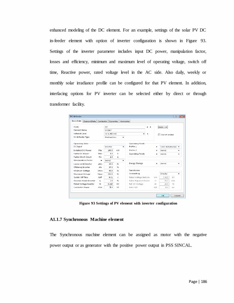
Page | 186
enhanced modeling of the DC element. For an example, settings of the solar PV DC
in-feeder element with option of inverter configuration is shown in Figure 93.
Settings of the inverter parameter includes input DC power, manipulation factor,
losses and efficiency, minimum and maximum level of operating voltage, switch off
time, Reactive power, rated voltage level in the AC side. Also daily, weekly or
monthly solar irradiance profile can be configured for that PV element. In addition,
interfacing options for PV inverter can be selected either by direct or through
transformer facility.
Figure 93 Settings of PV element with inverter configuration
A1.1.7 Synchronous Machine element
The Synchronous machine element can be assigned as motor with the negative
power output or as generator with the positive power output in PSS SINCAL.

Page | 187
Figure 94 Settings of the Power unit generator
The parameters setting for the generator which is shown in Figure 94 includes rated
apparent power, rated voltage, ratio of resistance and reactance (R/X), sub transient
reactance (xd”), internal reactance (xl). In addition, setting parameters for generator
transformer unit can be entered. Also an operating state of generator can be
determined according to the type of load flow calculations.
A1.1.8 Node/Bus bar
The node is a basic element in the power system network. Other branch elements
such as; transformer, line, etc. and node elements like; supply sources, consumers
are connected to the nodes. Bus bar is a graphical form of the node and the branch
elements can be connected between two or three bus nodes together.

Page | 188
A1.2 Selection of the calculation methods
In PSS SINCAL, type of simulation tool can be assigned by means of selecting
appropriate calculation methods in the asymmetrical network model. Load flow
analysis can be done with the advanced calculation methods such as; optimization,
low voltage dimensioning, harmonics and ripple control, etc. For PQ impacts
analysis in the proposed MG network model, load flow analysis (balanced and
unbalanced network), and harmonic analysis can be considered.
A1.2.1 Settings for LF calculation
In PSS SINCAL, currents in the network can be calculated on the basis of difference
in potential of nodes and the impedance between nodes. Current or voltage between
the nodes can be evaluated through the load flow analysis. The nodal point linear
expression can be written as per the equation (68):
Y*V = Ī, (68)
where Y is the admittance of nodal point, V is the vector of node voltages, and Ī is
the vector of currents.
Load flow analysis in PSS SINCAL can be done through the several calculation
procedures like; Admittance matrix, Newton Raphson method, unbalanced type, and
current iteration method. In this study, Newton Raphson method of LF analysis has
been considered for the proposed MG network model. The settings for load flow
analysis as shown in Figure 95, includes load flow procedure (Newton Raphson),
required number of iteration, power accuracy, voltage limit, and element utilization

Page | 189
limit. Controller activation options for the transformer (tap changer) and generator
unit along with the load shedding operation can also be added. In load flow
extension, it is possible to assign start time and duration of analysis over the period
of load profile.
Figure 95 Settings for the LF calculation
A1.2 .2 Settings for the unbalanced LF calculation
This meth od of calculation can be applied for a network with inclusion of
asymmetrical equipment and asymmetrical network elements. It is required to
consider additional phase sequence (zero/positive/negative) data for this
asymmetrical network simulation. Figure 9 6 shows the input settings for unbalanced
LF calculation which can be set according to the various standards like; V2/V1,
NEMA, IEC 61000 - 2 - 2, IEC 61000 - 2 - 4, etc.

Page | 190
Figure 96 Settings for the unbalanced LF calculation
Network elements can be defined for the unbalanced data by changing their
connection type. All the elements belonging to the symmetrical (all phases) type can
be converted into asymmetrical by means of changing connection among the phases.
For an example, there are options to change the phase connection of a load element
which is shown in Figure 97. During the simulation, PSS SINCAL gives the output
results of unbalanced load calculations (currents, voltages) for each phase.
Figure 97 Settings of the load element connection

Page | 191
A1.2.3 Settings for the Harmonics calculation
In PSS SINCAL, harmonics module calculates the distribution of harmonics in the
network and also calculating the level of frequency response. Calculation of
harmonic currents and voltages in the network can be evaluated using several
methods like; IEEE 519 standard, Telephone High Frequency Factor (THFF), IEC
61000-2-4 class1, etc. The settings for harmonics calculation which is shown in
Figure 98 includes different methods for harmonic calculation and also has options
to consider for the network resonance frequency level and voltage angle. In PSS
SINCAL, harmonics can be calculated on the basis of network impedance between a
defined starting frequency and an end frequency with appropriate frequency step. In
addition, for harmonics calculation, supplementary harmonic data (with respective
frequency) of specific voltage or current source element is required.
Figure 98 Settings of the harmonics calculation

Page | 192
A1.3 Main input data for the network model
Three main input data profiles are required to perform LF analysis and harmonic
analysis in the developed network model. They are; load data for connected load
which is based on daily load profile, solar data for connected PV which is based on
daily solar irradiance profile, and harmonic data for specific PV inverters and non-
linear load connected in network.
A1.3.1 Load data for daily load profile
Load profile data can be used to perform load curve or time varying simulation.
Load data for a connected load can be entered in per unit value over the daily or
weekly or yearly series of time frame. As shown in Figure 99, the settings of input
load data for a typical load profile represents the load power (per unit) variation over
the daily series of time frame (24 hours).
Figure 99 Typical daily load profile with input settings of load data

Page | 193
A1.3 .2 Solar data for daily solar profile
For a solar energy profile, solar irradiance data can be entered in per unit value over
the daily series of time frame. In addition, entering of solar data as per the typical
cloud pattern which affects the solar irradiance can also be done in PSS SINCAL. By
implementing solar disturbance in the solar profile , impacts level in the MG network
due to PV power variation can be identified during the simulation. Typical daily
solar profile with normal solar versus solar profile with solar disturbance is shown in
Figure 100 .
Figure 100 Typical daily solar profile (normal solar versus solar disturbance)
A1.3 .3 Current harmonic data for PV inverters and non - linear load
In order to analyze the harmonic distortion in the MG network, it is necessary to
enter harmonic emission data for the specific PV inverter and non - linear load which
are connected in the network. Standard limit of Harmonic emission data sp ecified by
the manufacturers of PV inverter can be considered for the harmonic analysis. Figure
101 shows the input window of current harmonics data entry and corresponding
harmonics current curve of the PV inverter.

Page | 194
Figure 101 harmonics current data and current curve of PV inverter
Non-linear load is one of the main sources for the harmonics current emission in the
network. The non-linear equipment‟s are classified into four groups such as; class-A,
B, C, and D. In this study, current harmonics of PV inverter and current harmonics of
class-A load have been considered during the harmonics analysis in the proposed
MG network model.

Page | 195
Appendix B
B1 Formulation of error signals for optimization
VSI control circuit of DG units (PV units and battery) which is shown in Figure 102
includes three main controllers namely; droop controller, voltage controller (Vd, Vqcontrol
loops), and current controller. As per the proposed control objectives, three error signals (Ea,
Eb, Ec) were formulated from each control loop. For optimizing control parameters of
voltage controller, formulation of error signals (Ea and Eb) of Vd (d-axis) and Vq (q-axis)
control loop are shown in Figure 103 and Figure 104 respectively. Similarly, for optimizing
inequality constraint of frequency variation, formulation of frequency error signal (Ec) is
shown in Figure 105.
Figure 102 Main control circuit of VSI

Page | 196
Figure 103 Voltage (Vd) control loop with formulation of error signal Ea
Figure 104 Voltage (Vq) control loop with formulation of error signal Eb

Page | 197
Figure 105 Formulation of frequency error signal Ef
Matlab work space signals which are assigned duri ng the process of optimization is
shown in Figure 106 .
Figure 106 Matlab work space signals (Optimization)