power distribution system tools for analyzing impacts of
TRANSCRIPT

Portland State University Portland State University
PDXScholar PDXScholar
Dissertations and Theses Dissertations and Theses
2-23-2021
Power Distribution System Tools for Analyzing Power Distribution System Tools for Analyzing
Impacts of Projected Electric Vehicle Load Growth Impacts of Projected Electric Vehicle Load Growth
Using GridLab-D Using GridLab-D
Shahad Alomani Portland State University
Follow this and additional works at: https://pdxscholar.library.pdx.edu/open_access_etds
Part of the Power and Energy Commons
Let us know how access to this document benefits you.
Recommended Citation Recommended Citation Alomani, Shahad, "Power Distribution System Tools for Analyzing Impacts of Projected Electric Vehicle Load Growth Using GridLab-D" (2021). Dissertations and Theses. Paper 5681. https://doi.org/10.15760/etd.7553
This Thesis is brought to you for free and open access. It has been accepted for inclusion in Dissertations and Theses by an authorized administrator of PDXScholar. Please contact us if we can make this document more accessible: [email protected].

Power Distribution System Tools for Analyzing Impacts of Projected Electric Vehicle Load
Growth Using GridLab-D
by
Shahad Alomani
A thesis submitted in partial fulfillment of therequirements for the degree of
Master of Sciencein
Electrical and Computer Engineering
Thesis Committee:Robert Bass, ChairRichard Campbell
John M. Acken
Portland State University2021

© 2021 Shahad Alomani

Abstract
The increased penetration of Electric Vehicle (EV) will provide substantial benefits to the
environment. However, each EV will present a significant additional load to electric power
distribution infrastructure, especially to radial distribution feeders. The additional load
may cause transformers to operate beyond their thermal limits, unacceptable voltage drops
along distribution lines, and primary conductor overloads. It is now, more than ever, vital
to understand the limitations of existing infrastructure in light of an accelerating push for
greener alternatives with insight that stems from modeling, simulation, and proper analysis
as the backbone to a well-informed response.
The objective of this work is to develop EV load growth modeling and analysis tools
for distribution systems. These tools will help researchers and distribution engineers better
understand the impacts EV growth will have on distribution systems. Such studies can help
a utility company take appropriate action to enhance grid stability and reliability. In the
following pages, three analysis tools for evaluating impacts of EV on grid infrastructure
assets are presented. These tools are developed for use in the GridLAB-D modeling
environment and written using Python 3.8.
The analysis tools were developed to serve unique purposes. The first tool notifies a
user of voltage violations. The second tool identifies conductor overloads. The third tool
alerts the user of transformer overloads. These tools have been evaluated using the IEEE
i

13 node test feeder coupled with typical household load profiles within GridLAB-D. Using
these tools, users evaluate the impacts EV loads have on distribution systems, specifically
transformer overloading, voltage violations, and the overload of conductors. These tools
can help utility distribution planners prepare appropriate response for anticipated EV load
growth.
ii

Dedication
For my mom and grandma who never stopped believing in me.
iii

Acknowledgements
Throughout the thesis research work and the thesis dissertation writing, I am pleased to
receive support, assistance and love from family, friends, and professors. Without their help,
I couldn’t accomplish this work.
I would first like to thank my advisor and the committee chair, Dr. Robert Bass, for his
patience, immense support and knowledge. His guidance helped me to be a better researcher.
Thank you for allowing me to be a part of the power lab research team. I would also like
to acknowledge Midrar Adham and Mohammed Alsaid for the hard work they put on this
thesis work. This work wouldn’t be possible without them.
I can’t leave Portland State without mentioning Ali Sheikly and William Isidort, Thank
you for the knowledge and support you have given me throughout the graduate classes.
Thank you for being always there for me when I needed it.
My deepest appreciation goes to my mother, grandmother, Fadilah and Mohammed, my
siblings, for their support and love for the past years, Thank you for believing in me. A
special thanks go to my closest friend Eman Albarazi who never gives up on me even when
I disappeared from her life, Thank you for always being my supportive friend.
Finally, I would also like to express my sincere gratitude to Dr. Richard Campbell and
Dr. John Acken for joining my thesis committee and the time you have put into my thesis.
iv

Acronyms
AAC All Aluminum Conductor. 35, 42, 61
AC Alternating Current. 9
ANSI American National Standards Institute. ix, 3, 12, 31, 32, 35–37, 44–46,
52, 57, 68
AWG American Wire Gauge. 34, 35, 42, 61
BESS Battery Energy Storage Systems. 5
CSV Comma Separated Values. 33, 35, 44, 48
DC Direct Current. 9, 10
DCFC DC Fast Charging. 10, 70
DER Distributed Energy Resources. 5
DOE Department of Energy. 4
EIA Energy Information Administration. 27
EPRI Electric Power Research Institute. 4
EV Electric Vehicle. i, ii, xi, xii, 2–10, 12, 27, 29, 30, 34, 38–40, 42, 45, 52,
54, 55, 57, 59–61, 63, 64, 66–71
EVSE Electric Vehicle Supply Equipment. 6, 8–10
FBS Forward-Backwards Sweep. 5, 18
v

GHG Greenhouse Gas. 1, 2
GMR Geometric Mean Radius. 19
GS Gauss-Seidel. 18
HELICS Hierarchical Engine for Large-scale Infrastructure Co-Simulation. 70
HVAC Heating, Ventilation, and Air Conditioning. 27
IEEE Institute of Electrical and Electronics Engineers. ix, xi–xiii, 3, 7, 12,
14–18, 21, 23, 25, 27, 35, 36, 38–41, 43–47, 49, 54, 55, 59, 61, 66–68, 76
IRP Integrated Resource Planning. 2
NEC National Electrical Code. 3, 13, 34, 35
NR Newton-Raphson. 5, 18
OpenDSS Open Distribution System Simulator. 4, 5
PES Power Engineering Software. 4
PEV Plug-in Electric Vehicle. 29
PGE Portland General Electric. 2, 6
PHEV Plug-in Hybrid Electric Vehicles. 6
PNNL Pacific Northwest National Laboratory. 4
PQ Power Quality. 7, 8
PV Photovoltaics. 5
RECS Residential Energy Consumption Survey. 27, 29
SoC State of Charge. 29
TE Transportation Electrification. 1, 2
vi

THD Total Harmonics Distortion. 8, 9
vii

Contents
Abstract i
Dedication iii
Acknowledgements iv
List of Tables xi
List of Figures xii
1 Introduction 11.1 Problem Statement . . . . . . . . . . . . . . . . . . . . . . . . . . . . . . 11.2 Objectives of Work . . . . . . . . . . . . . . . . . . . . . . . . . . . . . . 2
2 Literature Review 42.1 Power Engineering Software . . . . . . . . . . . . . . . . . . . . . . . . . 4
2.1.1 GridLAB-D . . . . . . . . . . . . . . . . . . . . . . . . . . . . . . 42.1.2 OpenDSS . . . . . . . . . . . . . . . . . . . . . . . . . . . . . . . 5
2.2 Impact of EVSE on Electric Power Distribution Infrastructure . . . . . . . 62.2.1 Distribution Transformers . . . . . . . . . . . . . . . . . . . . . . 62.2.2 Power Quality . . . . . . . . . . . . . . . . . . . . . . . . . . . . . 7
2.2.2.1 Voltage Drop . . . . . . . . . . . . . . . . . . . . . . . . 72.2.2.2 Harmonic Distortion . . . . . . . . . . . . . . . . . . . . 8
2.3 Electric Vehicle Service Equipment . . . . . . . . . . . . . . . . . . . . . . 92.3.1 Level 1 and 2 Chargers . . . . . . . . . . . . . . . . . . . . . . . . 92.3.2 Level 3 Chargers . . . . . . . . . . . . . . . . . . . . . . . . . . . 10
3 Design Considerations 113.1 Power Distribution Tools . . . . . . . . . . . . . . . . . . . . . . . . . . . 113.2 Voltage Violation Tool . . . . . . . . . . . . . . . . . . . . . . . . . . . . 123.3 Current Violation Tool . . . . . . . . . . . . . . . . . . . . . . . . . . . . 133.4 Transformer Overloading Tool . . . . . . . . . . . . . . . . . . . . . . . . 13
4 Tool Development 154.1 Power Distribution Tools . . . . . . . . . . . . . . . . . . . . . . . . . . . 15
viii

4.1.1 IEEE 13 Node Test Feeder Modeling . . . . . . . . . . . . . . . . . 154.1.1.1 Simulation Time . . . . . . . . . . . . . . . . . . . . . . 174.1.1.2 Modules . . . . . . . . . . . . . . . . . . . . . . . . . . 184.1.1.3 Configurations . . . . . . . . . . . . . . . . . . . . . . . 194.1.1.4 Objects . . . . . . . . . . . . . . . . . . . . . . . . . . . 23
4.1.2 Household Load Modeling . . . . . . . . . . . . . . . . . . . . . . 254.1.3 Household EV Modeling . . . . . . . . . . . . . . . . . . . . . . . 29
4.2 Voltage Violations Tool . . . . . . . . . . . . . . . . . . . . . . . . . . . . 314.2.1 ANSI C84.1 Standard . . . . . . . . . . . . . . . . . . . . . . . . . 32
4.3 Current Violations Tool . . . . . . . . . . . . . . . . . . . . . . . . . . . . 334.3.1 Overhead Distribution Lines . . . . . . . . . . . . . . . . . . . . . 344.3.2 NEC Standard . . . . . . . . . . . . . . . . . . . . . . . . . . . . . 34
4.4 Transformer Overloading Tool . . . . . . . . . . . . . . . . . . . . . . . . 354.4.1 IEEE / ANSI C57.96 Standard . . . . . . . . . . . . . . . . . . . . 36
5 Tool Validation 385.1 Power Distribution Tools . . . . . . . . . . . . . . . . . . . . . . . . . . . 38
5.1.1 IEEE 13 Node Test Feeder . . . . . . . . . . . . . . . . . . . . . . 395.1.2 Base Case . . . . . . . . . . . . . . . . . . . . . . . . . . . . . . . 395.1.3 EV Case . . . . . . . . . . . . . . . . . . . . . . . . . . . . . . . . 42
5.2 Voltage Violations Tool . . . . . . . . . . . . . . . . . . . . . . . . . . . . 445.3 Current Violations Tool . . . . . . . . . . . . . . . . . . . . . . . . . . . . 485.4 Transformer Overloading Tool . . . . . . . . . . . . . . . . . . . . . . . . 52
6 Discussion 546.1 Summer EV Test Case . . . . . . . . . . . . . . . . . . . . . . . . . . . . 54
6.1.1 Voltage Violations Tool . . . . . . . . . . . . . . . . . . . . . . . . 556.1.2 Current Violations Tool . . . . . . . . . . . . . . . . . . . . . . . . 61
6.2 Winter EV Test Case . . . . . . . . . . . . . . . . . . . . . . . . . . . . . 676.2.1 Transformer Overloading Tool . . . . . . . . . . . . . . . . . . . . 67
7 Conclusion 70
Bibliography 72
Appendix A: Tables 76A.1 Transformers and houses distributed along IEEE 13 node test feeder . . . . 76
A.1.1 Single phase node . . . . . . . . . . . . . . . . . . . . . . . . . . . 76A.1.2 Two phase nodes . . . . . . . . . . . . . . . . . . . . . . . . . . . 77A.1.3 Three phase nodes . . . . . . . . . . . . . . . . . . . . . . . . . . 78
A.2 Python Code . . . . . . . . . . . . . . . . . . . . . . . . . . . . . . . . . . 81A.2.1 Voltage Violation Tool . . . . . . . . . . . . . . . . . . . . . . . . 81A.2.2 Current Violation Tool . . . . . . . . . . . . . . . . . . . . . . . . 84
ix

A.2.3 Transformer Overloading Tool . . . . . . . . . . . . . . . . . . . . 87A.3 IEEE 13 Node Test Feeder Model in GridLAB-D . . . . . . . . . . . . . . 95
A.3.1 Input Data Files . . . . . . . . . . . . . . . . . . . . . . . . . . . . 95A.3.2 Glm Files . . . . . . . . . . . . . . . . . . . . . . . . . . . . . . . 95
x

List of Tables
4.1 IEEE 13 node test feeder transformer data . . . . . . . . . . . . . . . . . . . . 214.2 Total houses distributed along the IEEE 13 node test feeder model . . . . . . . 254.3 Number of transformers and houses attached to node 611 . . . . . . . . . . . . 264.4 Number of transformers and houses attached to node 633 . . . . . . . . . . . . 264.5 Power consumption specification . . . . . . . . . . . . . . . . . . . . . . . . . 274.6 EV penetration level with number of EV added to each house . . . . . . . . . . 30
5.1 Voltage violation events . . . . . . . . . . . . . . . . . . . . . . . . . . . . . . 465.2 Line 5 current violation events . . . . . . . . . . . . . . . . . . . . . . . . . . 505.3 Lines 6,7 and 8 current violation events . . . . . . . . . . . . . . . . . . . . . 515.4 Overloaded transformers events . . . . . . . . . . . . . . . . . . . . . . . . . . 52
xi

List of Figures
1.1 2018 US GHG emissions by sector . . . . . . . . . . . . . . . . . . . . . . . . 1
2.1 Voltage drop during EV charging in the secondary service . . . . . . . . . . . . 8
4.1 IEEE 13 nodes one line diagram . . . . . . . . . . . . . . . . . . . . . . . . . 164.2 Modified IEEE 13 nodes one line diagram . . . . . . . . . . . . . . . . . . . . 164.3 Structure of GridLAB-D distribution model . . . . . . . . . . . . . . . . . . . 174.4 Structure of Objects developed in GridLAB-D . . . . . . . . . . . . . . . . . . 244.5 Type 1 and Type 2 summer load profiles . . . . . . . . . . . . . . . . . . . . . 284.6 Type 1 and Type 2 winter load profiles . . . . . . . . . . . . . . . . . . . . . . 284.7 Winter EV load profile . . . . . . . . . . . . . . . . . . . . . . . . . . . . . . 294.8 Summer EV load profile . . . . . . . . . . . . . . . . . . . . . . . . . . . . . 304.9 Voltage violations tool flow chart . . . . . . . . . . . . . . . . . . . . . . . . . 314.10 ANSI C84.1 Voltage Ranges . . . . . . . . . . . . . . . . . . . . . . . . . . . 324.11 Current violations tool flow chart . . . . . . . . . . . . . . . . . . . . . . . . . 334.12 Transformer overloading tool flow chart . . . . . . . . . . . . . . . . . . . . . 36
5.1 Input-output diagram of IEEE 13 node test feeder model . . . . . . . . . . . . 395.2 Base case simulated current data on three transformers connect to Node 675 of
the IEEE 13 node test feeder model (Winter) . . . . . . . . . . . . . . . . . . . 405.3 Base case simulated Apparent Power data on three transformers connect to
Node 675 of the IEEE 13 node test feeder model (Winter) . . . . . . . . . . . . 415.4 Base case simulated Voltage data on three transformers connect to Node 675 of
the IEEE 13 node test feeder model (Winter) . . . . . . . . . . . . . . . . . . . 415.5 EV case simulated current data on three transformers connect to Node 675 of
the IEEE 13 node test feeder model (Winter) . . . . . . . . . . . . . . . . . . . 435.6 EV case simulated Apparent Power data on three transformers connect to Node
675 of the IEEE 13 node test feeder model (Winter) . . . . . . . . . . . . . . . 435.7 EV case simulated Voltage data on three transformers connect to Node 675 of
the IEEE 13 node test feeder model (Winter) . . . . . . . . . . . . . . . . . . . 445.8 Input-output diagram of Voltage Violation tool . . . . . . . . . . . . . . . . . . 455.9 Base case measured voltage of lines 1 and 3 of IEEE 13 node test feeder model 455.10 Base case measured voltage of lines 5 and 8 of IEEE 13 node test feeder model 465.11 EV case measured voltage of lines 1 and 3 of IEEE 13 node test feeder model . 475.12 EV case measured voltage of lines 5 and 8 of IEEE 13 node test feeder model . 47
xii

5.13 Input-output diagram of Current Violation tool . . . . . . . . . . . . . . . . . . 485.14 EV case measured current of lines 5 and 6 of IEEE 13 node test feeder model . 495.15 EV case measured current of lines 7 and 8 of IEEE 13 node test feeder model . 495.16 Input-output diagram of Transformer Overloading tool . . . . . . . . . . . . . 525.17 20 and 15 kVA transformers overloading events . . . . . . . . . . . . . . . . . 53
6.1 Base case of Lines 1 and 2 of Node 652 with no EV loads . . . . . . . . . . . 566.2 Voltage violation detected in lines 1 and 2 of Node 652 with 40% EV . . . . . . 566.3 Voltage violation detected in lines 1 and 2 of Node 652 with 60% EV . . . . . . 586.4 Voltage violation detected in lines 3 and 4 of Node 652 with 60% EV . . . . . . 586.5 Voltage violation events histogram at Node 652 . . . . . . . . . . . . . . . . . 596.6 20% EV with no voltage violations compared with base case with no EV in line
1 of Node 652 . . . . . . . . . . . . . . . . . . . . . . . . . . . . . . . . . . . 606.7 Voltage violations detected in line 1 of Node 652 with 40% - 100% EV . . . . . 606.8 Current violations detected in lines 1 and 4 of Node 646 with 40% EV . . . . . 626.9 Current violations detected in lines 5 and 6 of Node 646 with 40% EV . . . . . 626.10 Current violations detected in lines 1 and 4 of Node 646 with 60% EV . . . . . 636.11 Current violations detected in lines 7 and 8 of Node 646 with 60% EV . . . . . 646.12 Current violations detected in lines 1 and 4 of Node 646 with 80% EV . . . . . 656.13 Current violations detected in lines 5 and 6 of Node 646 with 80% EV . . . . . 656.14 Current violations detected in lines 7 and 8 of Node 646 with 80% EV . . . . . 666.15 Transformer overloading events histograms at Node 692 phase A . . . . . . . 686.16 Transformer overloading events histograms at Node 692 phase B . . . . . . . . 696.17 Transformer overloading events histograms at Node 692 phase C . . . . . . . . 69
xiii

1 Introduction
1.1 Problem Statement
The transportation sector accounts for the largest share of the total Greenhouse Gas (GHG)
emissions, at 28% as shown in Figure 1.1 [1]. Most of the GHG emissions from transporta-
tion come from burning fossil fuels for passenger vehicles, which accounts for 65% of the
global emissions [2]. The most valuable path to reduce GHG emissions and fossil fuel de-
pendence is Transportation Electrification (TE). However, the approach to the electrification
of transportation is not without challenges. For GHG emissions reduction to succeed, most
energy sources for electricity need to derive from low carbon resources, such as solar and
wind power plant.
Figure 1.1: 2018 US GHG emissions by sector [1]
1

Utilities are planing to meet the goal of reducing GHG emissions, in part, by preparing
for TE. For instance, Portland General Electric (PGE) plans to electrify at least 60% of
their entire vehicle fleet by 2030 [3]. Regardless of the benefits of TE, the increased
adoption of EV poses considerable concerns. High load growth due to EV penetration
potentially add high power consumption and therefore high demand to the total power
supplied. Considering the number of EVs anticipated to be charging during peak hours,
the risk of overloading distribution transformers is exceptionally high in the summer and
winter seasons due to loading from air conditioning and electric heating units, respectively.
Distribution transformers need to function within their thermal limits to avoid decreasing
their mean time to failure, and to maintain grid stability and reliability. Thus, transformer
overloading, voltage drops along distribution lines, and primary conductor overloads must
be studied and analyzed. For this research, multiple analysis tools were developed to
study distribution transformers overloading, voltage violations, and overloading of primary
conductors as impacted by anticipated EV loading.
1.2 Objectives of Work
As EV adoption grows, utilities need to familiarize themselves with EV load growth impacts.
Generally, utilities plan for asset upgrades to compensate for future load growth by conduct-
ing Integrated Resource Planning (IRP). Utilities determine the risks associated with power
demand and supply that meet future requirements and government policies. The motivation
for this thesis work is to understand, analyze, and develop tools on power distribution
2

systems that indicate voltage violations, transformer overloads, and proper conductor size.
A deeper understanding of EV impacts will aid utilities in the planning process of power
system distribution infrastructure upgrades by providing data imperative to scheduling these
improvements.
The tools developed in this thesis, in part, address the impacts that EV load growth will
have on distribution transformers. Most distribution transformers operate at high average
efficiency where temperature and air quality impact transformers functionality over time.
The distribution transformer tool developed in this thesis work indicates the overload time
and apparent power rates compared with the Institute of Electrical and Electronics Engineers
(IEEE) C57.96 standard [4]. Voltage drops along distribution lines must be within the
service voltage limits, as stated by the American National Standards Institute (ANSI) C84.1
standard [5]. Therefore, the voltage drop tool was developed to indicate the voltage drop
along the transmission line associated with the distribution transformers. The third and
final tool is the conductors sizing tool, which was designed to show if the conductor current
exceeds the primary conductor sizing established by the National Electrical Code (NEC).
The tools developed for this thesis will provide asset distribution planners tools for analyzing
distribution system impacts due to projected EV load growth and to position their utilities
for future planning.
3

2 Literature Review
2.1 Power Engineering Software
Analyzing EV impact on a power distribution system requires an appropriate simulation
environment. There are several Power Engineering Software (PES) available in the market
that simulate smart grid technologies. Power engineers rely on PES to perform distribution
system analysis. GridLAB-D and OpenDSS are examples of open-source PES. These
are associated with Pacific Northwest National Laboratory (PNNL) and Electric Power
Research Institute (EPRI), respectively. Utilities widely use ETAP and CYMDIST, which
are commercially available. These commercial PES are usually prohibitively expensive for
university research. Although the vast majority of the software capabilities are comparable,
they are diverse in their features. After comparing the capabilities of GridLB-D and
OpenDSS, GridLAB-D was chosen as the distribution system PES for this thesis work. In
the following sections, a comparison between OpenDSS and GridLAB-D is presented.
2.1.1 GridLAB-D
GridLAB-D is a power distribution system analysis and simulation tool developed at the
behest of US Department of Energy (DOE) by PNNL [6]. GridLAB-D provides several
capabilities for modeling distribution systems and renewable energy, from generation to
4

end-use models, including appliance and equipment models. Furthermore, GridLAB-D is
capable of modeling Distributed Energy Resources (DER), which include Photovoltaics
(PV), wind turbines, Battery Energy Storage Systems (BESS), and EVs. It also provides
various modeling capabilities such as distribution power flow analysis, energy market
simulation and residential load modeling [6]. GridLAB-D was used as the simulation
environment for the distribution system tools for numerous reasons. Beginning with the first
reason, it is open source. Besides, GridLAB-D is widely used by industry and universities.
It is considered a valuable tool for modeling distribution feeders [7] [8].
2.1.2 OpenDSS
Open Distribution System Simulator (OpenDSS) is a power system simulation tool devel-
oped by Electrotek Concepts in 1997 before EPRI took over in 2014. OpenDSS supports
power flow analysis, harmonic analysis, and smart grid simulation [9]. While being open-
source with all distribution system simulation features, OpenDSS was not chosen for the tool
validation for several reasons. OpenDSS uses a frequency-based analysis instead of time
analysis, unlike the other software OpenDSS uses impedance matrix analysis and a current
injection method to solve current and voltage values [9]. A non-linear system resolution algo-
rithm in distribution system nodes such as Newton-Raphson (NR) and Forward-Backwards
Sweep (FBS) method is needed to validate the nodes and loads distribution for the developed
tools.
5

2.2 Impact of EVSE on Electric Power Distribution Infrastructure
The absence of proper planning to integrate EV load growth may lead to an additional burden
on power distribution infrastructure, especially to radial distribution feeders. Furthermore,
EV charging during peak hours poses several challenges for distribution systems. These
challenges include power quality issues, such as voltage drop and harmonics, transformer
overloading, and conductor resizing. EV is defined as a vehicle that operates on an electric
motor rather than an internal combustion engine. Each EV needs Electric Vehicle Supply
Equipment (EVSE), which is the equipment used for supplying EVs with electricity. As
part of understanding the impact of EVSE, a literature review of EVSE charging impact on
distribution infrastructure assets is presented.
2.2.1 Distribution Transformers
Distribution transformers are one of the most prolific distribution infrastructure components,
connecting hundreds of thousands of residential homes to the power grid. For example,
PGE, which is a midsize utility, has over 150,000 distribution transformers within its
balancing area. Therefore, studying the impact of EVSE on distribution transformers is a key
consideration when modeling EVSE impact. Substantial research exists concerning EVSE
charging impacts on distribution transformers. Shao et al., demonstrated that Plug-in Hybrid
Electric Vehicles (PHEV) charging during peak hours would overload a 25 kVA distribution
transformer by 103% during winter, and 98% during summer [10]. Shao et al., speculate that
if the charging scenario is uncoordinated during peak hours, distribution transformer needs
6

to be upgraded to meet the load growth. Research by Hilshey et al., focused on the aging of
a 25 kVA service transformer experimented with six EVs and while considering ambient
temperature for a transformer based on IEEE standard and multiple charging scenarios [11].
It is indicated that with a high level of EV adoption, transformer aging is accelerated.
2.2.2 Power Quality
Power Quality (PQ) issues such as voltage drop and harmonic distortion within distribution
feeders due to the increase of non-linear loads are of concern. EV chargers are non-linear
loads, which may present a higher impact due to harmonics produced by their power
electronics. Analyzing voltage drops within the feeder voltage due to increased EV load
growth is essential to ensure distribution system reliability and stability because voltages
must be maintained within specified tolerances in order to ensure loads can stay online. The
following sections introduce the background of EV load growth impact on voltage drop and
harmonic distortion.
2.2.2.1 Voltage Drop
As the load on the distribution feeder diverges, so does the voltage drop between the sub-
station and the end-user. To maintain the end-user voltage within acceptable range, the
substation voltage needs to be regulated. Therefore, analyzing the voltage drops along distri-
bution lines is important. Significant analysis on distribution feeders has been performed
concerning the impact of EV load on distribution lines. Research by Dubey and Santoso
[12] analyzed the effect of EV charging on distribution voltage with a 13.8 kV distribution
7

feeder. Results show that by installing EVSE with a single EV charging, the load leads to a
voltage drop of 4.41%, as shown in Figure 2.1. Taylor et al., showed that additional EV load
growth repeatedly will raise the voltage regulation in primary distribution lines [13].
Figure 2.1: Voltage drop during EV charging in the secondary service [12].
2.2.2.2 Harmonic Distortion
Harmonic distortion is one of the most common issues of PQ. Thus, it is important to
determine its impact, especially at the distribution level where EVSE are located. Several
studies have been carried out to analyze the harmonic implications for EV chargers [14],[15].
Harmonic distortion is defined as the ratio of the square root of the sum of the square of
harmonic magnitude to fundamental sine wave magnitude. It could be a deviation of a
current or voltage waveform. Most studies focus on the harmonic current due to its potential
impact on magnetic assets like distribution transformers and motors. The study by Ul-haq
et al., illustrates the importance of analyzing the harmonic distortion by modeling several
different EV penetration levels [14]. Results show that with light loading, the current Total
Harmonics Distortion (THD) is 5.6% while the voltage remain within acceptable limits.
8

However, with 95% EV penetration, voltage distortion exceeds the allowable THD limit by
8%.
2.3 Electric Vehicle Service Equipment
The function of EVSE is to properly supply EV with electricity for charging of the battery.
EVSE are commonly categorized into three different levels: Level 1, Level 2, and Level 3.
These groupings vary by power level. Levels 1 and 2 EVSE provide Alternating Current
(AC) power flow to the charger inside the vehicle. Level 3 charges the battery directly with
Direct Current (DC). In the following sections, a comparison of the three charger levels is
presented.
2.3.1 Level 1 and 2 Chargers
Level 1 chargers use a 120 V voltage supply connected to a 15 or 20 A receptacle with
a maximum current of 12 to 16 A. These chargers generally take 8 to 12 hours to fully
charge a vehicle. Therefore, EV owners with Level 1 EVSE typically charge their vehicles
overnight. Level 2 chargers are the preferable chargers since they take less time to charge
than Level 1 chargers. Level 2 chargers use a 208 V or 240 V input voltage with 32 to 80 A
maximum current depending on the charging station design. Level 2 chargers are commonly
used in residential areas and consume higher power than Level 1 chargers.
9

2.3.2 Level 3 Chargers
While most EV owners feel comfortable charging their vehicle at home by using either Level
1 or 2 EVSE , Level 3, known as DC Fast Charging (DCFC), is commonly used in industrial
and commercial areas, as they are costly and require specific equipment. Most Level 3
chargers require a 480 V DC service. Some DCFC are capable of charging a passenger
vehicle to 80% capacity in around 30 minutes.
10

3 Design Considerations
Design considerations are principles that provide methods to guide the development process
strategy and ultimately shape the final result. Design considerations are formulated to
generate focus on how the design requirements are met and, therefore, influence each tool
design. In the following sections, each of the design considerations are identified and their
application in the design of the Power Distribution tools are discussed.
Three tools were developed for this thesis work. These tools are designed for residential
loads with the consideration for EV load growth impact. The Voltage Violations tool
is designed to indicate voltage drops along the feeder line associated with distribution
transformers. The Current Violations tool is designed to indicate over-current events along
overhead lines. The Transformer Overloading tool is developed to indicates the percentage
of transformer overloading.
3.1 Power Distribution Tools
The purpose of developing the three Power Distribution tools (Voltage Violations, Current
Violations, and Transformer Overloading), is to help distribution planners analyze the impact
of EV load growth. For a given distribution system study, these tools monitor the impacts of
EV load growth on distribution lines and transformers.
11

These Power Distribution tools were created by following the guidance of three design
considerations. The first design consideration is how to create a model to test each of
the Power Distribution tools functionality. The second design consideration is how to
provide a method for adding and distributing residential loads to each household. The third
consideration is how to facilitate in the decision for the number of EV each household should
be included. Using the above design considerations as guidance, the following decisions are
made to facilitate the development of the three Power Distribution tools; the IEEE 13 node
was chosen as a test feeder, 1000 households were distributed among the test feeder nodes,
and each household included one EV distributed with the ability to modify the percentage
of EV penetration level for any given simulation.
3.2 Voltage Violation Tool
The Voltage Violations tool uses simulated voltage data to detect any voltage drop along
transmission lines and alerts the user when a limit has been exceeded. The simulated voltage
data input is the meter value between the service equipment and the household distribution
line for a given simulation. This tool ensures that the input voltage value lies within a
specific range.
In developing a tool that can identify voltage violations, two design considerations were
considered. The first consideration; the nominal voltage rating and operating standard being
used by utilities. The ANSI C84.1 standard for voltage violations range was found to be
used by utilities [5]. The second consideration; the optimal power system type to examine.
12

The optimal system to be examined is a distribution system.
3.3 Current Violation Tool
The Current Violations tool utilizes simulated current data to detect an over-current condition
along the conductors. The simulated current data input is the meter value between the service
equipment and the household for a given simulation. This tool flags a current violation for
overhead line conductors.
In developing a tool that can identify over-current conditions, two design considerations
were considered. The considerations are as follows: which conductors are to be considered
for current analysis, and the conductor sizing standard the utility employs in planning studies.
The conductors considered for analysis are overhead distribution lines and the conductor
sizing standard is NEC.
3.4 Transformer Overloading Tool
The Transformer Overloading tool indicates transformer overload conditions in distribution
systems. This tool uses simulated power data between distribution lines and household
loads, to alert a user when the output power exceeds the rating.
In developing a tool that can identify transformer overload conditions, two design
considerations were considered. The considerations are as follows: the transformer standard
used by utilities for monitoring transformer overload conditions, and the appropriate sizing
typically used for distribution transformers. The transformer overloading standard used
13

by utilities is the IEEE C57.96 to monitor each transformer overload percentage. The
transformer rating for distribution are sized at 15 kVA - 35 kVA, at increments of 5 kVA.
14

4 Tool Development
Tool development is the process of implementing design considerations. These sections
provide illustrations and detailed descriptions of the capabilities of each Power Distribution
tools. The subsections then discuss how each design consideration is realized.
4.1 Power Distribution Tools
Three design considerations were applied during the development of Power Distribution
tools. The first consideration is for choosing the appropriate test feeder model. The second
consideration is the distribution of households along with the nodes of the test feeder model.
The third consideration is adding EV loads, distributed among the households. An in-depth
description of each consideration is presented in the following subsections.
4.1.1 IEEE 13 Node Test Feeder Modeling
IEEE 13 node test feeder was chosen to evaluate Power Distribution tools functionalities.
Figure 4.1 is a one-line diagram of the IEEE 13 node test feeder selected for modeling
[16]. The feeder model includes overhead and underground lines, a voltage regulator,
and a substation transformer. For this thesis work, the feeder model was configured to
accommodate a set of 1000 households with their respective EV loads as a means to evaluate
EV load growth impact on the distribution transformers and lines. A distribution transformer
15

was added to each node, except for nodes 650 and 634. In the IEEE 13 node test feeder,
nodes 650 and 634 serve commercial loads. Figure 4.2 is the configured one line diagram of
the IEEE 13 node test feeder model with a distribution transformer, a household, and an EV
load connected to each node.
Figure 4.1: IEEE 13 nodes one line diagram [16]
Figure 4.2: Modified IEEE 13 nodes one line diagram with EV
16

The method for testing Power Distribution tool functions was accomplished through
modeling the configured IEEE 13 node test feeder in GridLAB-D [17]. GridLAB-D is a
command-line program, which uses simple text files as input for specific objects, classes,
and modules. The structure of creating a distribution feeder model in GridLAB-D is shown
in Figure 4.3. In the next subsection, a comprehensive description of each structural element
is included. It should be incorporated into the scripting code writing to model a distribution
system in GridLAB-D successfully.
Figure 4.3: Structure of GridLAB-D distribution model
4.1.1.1 Simulation Time
In GridLAB-D, the simulation time is set by a clock that defines a timestamp and time step.
The simulation time selected for the configured IEEE 13 node feeder model has a timestamp
of one week, with a time step at 10 minutes:
c l o c k {
t imes t amp '2010 −07 −25 0 : 0 0 : 0 0 ' ;
s t o p t i m e '2010 −07 −31 0 : 1 0 : 0 0 ' ;
t i m e z o n e PST+8PDT ;
}
17

4.1.1.2 Modules
GridLAB-D provides various types of modules to perform an analysis for a given model.
The configured IEEE 13 node test feeder model used to validate Power Distribution tools
requires three types of modules. The modules are; tape, power flow, and residential.
The tape module is used to implement player and recorder objects that modify boundary
conditions and identify object properties [18]. The power flow module is set to a specific
iterative calculation method to solve power flow quantities that provide steady-state node
voltage and line current. There are three power flow iterative calculation methods available
in GridLAB-D: NR, FBS, and Gauss-Seidel (GS). The iterative calculation method chosen
for distribution modeling is FBS. FBS was selected over NR and GS because FBS performs
the calculations in an efficient and accurate manner [19]. It is important to note that the
configured IEEE 13 node test feeder model is a radial system, and FBS is the preferred
method for solving three-phase unbalanced systems of this system type. The residential
module is used to provide classes for each household and simulate single-family homes.
The three modules used are configured as follows:
module t a p e ;
module powerf low {
s o l v e r _ m e t h o d FBS ;
d e f a u l t _ m a x i m u m _ v o l t a g e _ e r r o r 1e −9;
l i n e _ l i m i t s TRUE;
} ;
module r e s i d e n t i a l {
i m p l i c i t _ e n d u s e s NONE;
ANSI_vol tage_check TRUE;
} ;
18

4.1.1.3 Configurations
Configurations are used in GridLAB-D to describe each particular object implementation.
For example, each underground and overhead line, transformer, and voltage regulator is an
object and requires configurations that identify and define the parameters for each object. A
triplex is a type of object that sets parameters and is combined with other objects. A triplex
line conductor object was used to represent conductor configurations as follows:
o b j e c t t r i p l e x _ l i n e _ c o n d u c t o r {
name t r i p l e x _ l i n e _ c o n d u c t o r _ 1 ;
r e s i s t a n c e 0 . 9 7 ;
g e o m e t r i c _ m e a n _ r a d i u s 0 . 0 1 1 1 ;
} ;
o b j e c t t r i p l e x _ l i n e _ c o n f i g u r a t i o n {
name t r i p l e x _ l i n e _ c o n f i g u r a t i o n _ m a i n _ l i n e s ;
c o n d u c t o r _ 1 t r i p l e x _ l i n e _ c o n d u c t o r _ 1 ;
c o n d u c t o r _ 2 t r i p l e x _ l i n e _ c o n d u c t o r _ 1 ;
conduc tor_N t r i p l e x _ l i n e _ c o n d u c t o r _ 1 ;
i n s u l a t i o n _ t h i c k n e s s 0 . 0 8 ;
d i a m e t e r 0 . 3 6 8 ;
}
After triplex line conductors are configured, overhead and underground line conductor
configurations were listed together with the line spacing between the lines. Line spacing,
Geometric Mean Radius (GMR), distance, and resistance values were used as listed in [16].
Examples of the underground and overhead line configurations are shown below:
• Overhead line conductor configuration:
o b j e c t o v e r h e a d _ l i n e _ c o n d u c t o r :6010 {
19

g e o m e t r i c _ m e a n _ r a d i u s 0 . 0 3 1 3 ;
r e s i s t a n c e 0 . 1 8 5 9 ;
}
o b j e c t l i n e _ s p a c i n g :500601 {
d i s t ance_AB 2 . 5 ;
d i s t ance_AC 4 . 5 ;
d i s t ance_BC 7 . 0 ;
d i s t ance_BN 5 . 6 5 6 8 5 4 ;
d i s tance_AN 4 . 2 7 2 0 0 2 ;
d i s t ance_CN 5 . 0 ;
}
o b j e c t l i n e _ c o n f i g u r a t i o n :601 {
conduc tor_A o v e r h e a d _ l i n e _ c o n d u c t o r : 6 0 1 0 ;
conduc to r_B o v e r h e a d _ l i n e _ c o n d u c t o r : 6 0 1 0 ;
conduc to r_C o v e r h e a d _ l i n e _ c o n d u c t o r : 6 0 1 0 ;
conduc tor_N o v e r h e a d _ l i n e _ c o n d u c t o r : 6 0 2 0 ;
s p a c i n g l i n e _ s p a c i n g : 5 0 0 6 0 1 ;
}
• Underground line conductor configuration:
o b j e c t u n d e r g r o u n d _ l i n e _ c o n d u c t o r :6060 {
o u t e r _ d i a m e t e r 1 . 2 9 ;
conduc to r_gmr 0 . 0 1 7 1 ;
c o n d u c t o r _ d i a m e t e r 0 . 5 6 7 ;
c o n d u c t o r _ r e s i s t a n c e 0 . 4 1 ;
n e u t r a l _ g m r 0 . 0 0 2 0 8 0 0 ;
n e u t r a l _ r e s i s t a n c e 1 4 . 8 7 2 ;
n e u t r a l _ d i a m e t e r 0 . 0 6 4 0 8 3 7 ;
n e u t r a l _ s t r a n d s 1 3 . 0 ;
s h i e l d _ g m r 0 . 0 ;
s h i e l d _ r e s i s t a n c e 0 . 0 ;
20

}
o b j e c t l i n e _ s p a c i n g :515 {
d i s t ance_AB 0 . 5 0 ;
d i s t ance_BC 0 . 5 0 ;
d i s t ance_AC 1 . 0 ;
d i s tance_AN 0 . 0 ;
d i s t ance_BN 0 . 0 ;
d i s t ance_CN 0 . 0 ;
}
o b j e c t l i n e _ c o n f i g u r a t i o n :606 {
conduc tor_A u n d e r g r o u n d _ l i n e _ c o n d u c t o r : 6 0 6 0 ;
conduc to r_B u n d e r g r o u n d _ l i n e _ c o n d u c t o r : 6 0 6 0 ;
conduc to r_C u n d e r g r o u n d _ l i n e _ c o n d u c t o r : 6 0 6 0 ;
s p a c i n g l i n e _ s p a c i n g : 5 1 5 ;
}
Transformers are classified into two types, substation and distribution transformers. The
substation transformer used in IEEE 13 node test feeder is 5000 kVA. Values used to develop
substation transformer shown in Table 4.1. The configuration used to model transformers in
GridLAB-D for the distribution models shown below:
Table 4.1: IEEE 13 node test feeder transformer data
kVA kV- high kV- low R - % X - %Substation: 5,000 115 - D 4.16 Gr. Y 1 8XFM - 1: 500 4.16 – Gr.W 0.48 – Gr.W 1.1 2
• Substation Transformer Configuration:
o b j e c t t r a n s f o r m e r _ c o n f i g u r a t i o n :400 {
c o n n e c t _ t y p e WYE_WYE;
i n s t a l l _ t y p e PADMOUNT;
p o w e r _ r a t i n g 500 ;
21

p r i m a r y _ v o l t a g e 4160 ;
s e c o n d a r y _ v o l t a g e 480 ;
r e s i s t a n c e 0 . 0 1 1 ;
r e a c t a n c e 0 . 0 2 ;
}
Distribution transformer ratings used for the distribution feeder model vary between 15 kVA
and 35 kVA. An example of a 15 kVA single phase center tap transformer is shown below:
• Distribution Transformer Configuration:
o b j e c t t r a n s f o r m e r _ c o n f i g u r a t i o n {
name CS15_conf ig ;
c o n n e c t _ t y p e SINGLE_PHASE_CENTER_TAPPED ;
i n s t a l l _ t y p e POLETOP ;
p o w e r C _ r a t i n g 1 5 ;
p r i m a r y _ v o l t a g e 2401 ;
s e c o n d a r y _ v o l t a g e 1 2 0 . 0 0 0 ;
impedance 0 . 0 0 6+ 0 . 0 1 3 6 j ;
}
The last configuration in the GridLAB-D distribution feeder model structure is the voltage
regulator, which is used to hold the system voltage at 122 V.
o b j e c t r e g u l a t o r _ c o n f i g u r a t i o n :650 {
c o n n e c t _ t y p e WYE_WYE;
b a n d _ c e n t e r 1 2 2 . 0 0 0 ;
band_wid th 2 . 0 ;
t i m e _ d e l a y 0 . 0 ;
d w e l l _ t i m e 0 . 0 ;
r a i s e _ t a p s 1 6 ;
l o w e r _ t a p s 1 6 ;
c u r r e n t _ t r a n s d u c e r _ r a t i o 700 ;
22

p o w e r _ t r a n s d u c e r _ r a t i o 2 0 ;
c o m p e n s a t o r _ r _ s e t t i n g _ A 3 . 0 ;
c o m p e n s a t o r _ x _ s e t t i n g _ A 9 . 0 ;
c o m p e n s a t o r _ r _ s e t t i n g _ B 3 . 0 ;
c o m p e n s a t o r _ x _ s e t t i n g _ B 9 . 0 ;
c o m p e n s a t o r _ r _ s e t t i n g _ C 3 . 0 ;
c o m p e n s a t o r _ x _ s e t t i n g _ C 9 . 0 ;
CT_phase "ABC" ;
PT_phase "ABC" ;
C o n t r o l MANUAL;
c o n t r o l _ l e v e l INDIVIDUAL ;
Type A;
tap_pos_A 0 ;
tap_pos_B 0 ;
tap_pos_C 0 ;
r e g u l a t i o n 0 . 1 0 ;
}
o b j e c t r e g u l a t o r :650630 {
p h a s e s "ABCN" ;
from node : 6 5 0 ;
t o node : 6 3 0 ;
s e n s e _ n o d e N671 ;
c o n f i g u r a t i o n r e g u l a t o r _ c o n f i g u r a t i o n : 6 5 0 ;
}
4.1.1.4 Objects
Each object implemented in GridLAB-D is a specific instance of a class, and each class
is defined as a collection of algorithms, which determines how each object should behave
[20]. Objects used to develop the IEEE 13 node test feeder are as follows: nodes, lines,
23

transformers, houses, loads, meters, and recorders. The node object is a bus of the distri-
bution system that provides the connection point for the system voltage [20]. The voltage
developed in the node object operates as a three-phase voltage connected in wye or delta
connection. The triplex node object works on a split-phase level, and each triplex load phase
connects through a triplex node. The triplex load is used to vary the load value with time for
a given object. As shown in Figure 4.4, each distribution transformer connects to one of the
triplex nodes, and then houses were connected to each transformer through a triplex meter.
Triplex lines are established to connect two objects together. The triplex meter is used to
provide a measurement point of power, current, and voltage for downstream connections
[20]. Each triplex meter is coupled with a set of recorders. Recorders are utilized to collect
and save data from meter objects associated with them.
Figure 4.4: Structure of Objects developed in GridLAB-D
24

4.1.2 Household Load Modeling
In order to evaluate EV load growth impacts on distribution lines and transformers, a set of
household loads was distributed along the IEEE 13 node test feeder. The method for the
distribution of household loads applied for this dissertation was adopted from Ahourai and
Alfaruque, who considered distributing 1000 houses along IEEE 13 node test feeder [21].
By using this method, three to seven houses were attached to each distribution transformer.
Table 4.2 indicates the number of houses distributed for each phase of the IEEE 13 node test
feeder.
Table 4.2: Total houses distributed along the IEEE 13 node test feeder model
Phases Numbers of HousesPhase A 319Phase B 303Phase C 378
198 distribution transformers were distributed among the IEEE 13 node test feeder. Most
distribution transformers used by utilities are rated to serve between 15 to 50 kVA load.
Typically, these transformers serve 5 to 15 homes. For modeling purposes, transformers
were developed to serve three to seven houses and rated to serve between 15 to 35 kVA.
The 15 kVA transformer was used to serve three household and the 35 kVA serves seven
household. To model houses and transformers in GridLAB-D, 1000 houses were randomly
distributed among the IEEE 13 node test feeder. Each single-phase center tap transformer
attached to one of three, two, and single-phase nodes. The following tables illustrate how
each center tap transformers connected. Tables 4.3 and 4.4 show nodes 611 and 633, a
single-phase node and a three-phase node with several transformers and houses attached.
25

Table 4.3: Number of transformers and houses attached to node 611
IEEE 13 Nodes Phase Transformer Rating ( kVA) Number of Houses
Node 611 C
25 515 320 430 635 725 520 425 5
Table 4.4: Number of transformers and houses attached to node 633
IEEE 13 Nodes Phase Transformer Rating ( kVA) Number of Houses
Node 633
A
25 530 615 325 535 730 630 625 5
B
15 320 415 315 325 525 520 425 5
C
20 420 415 315 325 525 525 515 3
26

To evaluate the impact of EVs on lines and transformers connected with each EV and
household, it is necessary to have household demand profiles. The electricity demand
profiles used to model the IEEE 13 node test feeder was adopted from Muratori, who
generated a modeling method that produces power consumption patterns [22]. Data for
electricity demand are selected from the Residential Energy Consumption Survey (RECS)
[23]. Each individual household demand profile is composed of 200 households. Each
profile includes Heating, Ventilation, and Air Conditioning (HVAC) system data with 10
minutes resolution.
For modeling each household load profile in GridLAB-D, two load profile types were
identified. The first type represents lower power consumption households, and the second
type represents higher power consumption households. As reported by the Energy Infor-
mation Administration (EIA), the average annual electricity consumption for a residential
household was 10,649 kWh, which is about an average of 877 kWh per month [22]. There-
fore, the average power consumption was 1.200 kW per month. As a result, the two load
profile types have been chosen to be up to 3.5 kW for low power consumption and up
10 kW to represent higher power consumption. Table 4.5 shows the power consumption
specification for each type. Type 1 and Type 2 were randomly distributed among 1000
houses in GridLAB-D. An example of summer and winter load profiles are presented in
Figure 4.5 and Figure 4.6.
Table 4.5: Power consumption specification
Types Power Consumption ( kW )Type 1 1 - 3.5Type 2 3.6 - 10
27

Jul 25 Jul 26 Jul 27 Jul 28 Jul 29 Jul 30 Jul 31
Time 2010
0
2000
4000
6000
8000
10000
Pow
er
(W)
Summer Type 2 Load Profile
Jul 25 Jul 26 Jul 27 Jul 28 Jul 29 Jul 30 Jul 31
Time 2010
0
500
1000
1500
2000
2500
3000
Pow
er
(W)
Summer Type 1 Load Profile
Figure 4.5: Type 1 and Type 2 summer load profiles
Dec 25 Dec 26 Dec 27 Dec 28 Dec 29 Dec 30 Dec 31 Jan 01
Time 2010
2000
4000
6000
8000
Po
we
r (W
)
Winter Type 2 Load Profile
Dec 25 Dec 26 Dec 27 Dec 28 Dec 29 Dec 30 Dec 31 Jan 01
Time 2010
1000
2000
3000
4000
Po
we
r (W
)
Winter Type 1 Load Profile
Figure 4.6: Type 1 and Type 2 winter load profiles
28

4.1.3 Household EV Modeling
To accurately analyze EV impacts on distribution transformers and lines, EV load profile
data are used to characterize the load. All EV load profile data used in this work, acquired
from RECS, are randomly distributed among 1000 houses [23]. These profiles have been
generated using the modeling method proposed by Muratori et al., who considered generating
348 Plug-in Electric Vehicle (PEV) charging profiles for in-home charging [24]. Two
assumptions were made while developing these load profiles. The first assumption is the EV
were at 60% of State of Charge (SoC) for 200 mile range and 40% of SoC for 40 mile range.
The second assumption is the in-home charging station is a Level 2 charging station with
a maximum power of 6600 W. An illustration of winter and summer EV load profiles are
shown in Figures 4.7 and 4.8.
Dec 25 Dec 26 Dec 27 Dec 28 Dec 29 Dec 30 Dec 31 Jan 01
Time 2010
0
1000
2000
3000
4000
5000
6000
7000
Pow
er
(W)
Figure 4.7: Winter EV load profile
29

Jul 25 Jul 26 Jul 27 Jul 28 Jul 29 Jul 30 Jul 31 Aug 01
Time 2010
0
1000
2000
3000
4000
5000
6000
7000
Po
we
r (W
)
Figure 4.8: Summer EV load profile
For modeling EV impacts in GridLAB-D, five different penetration rates of EV were con-
sidered. Table 4.6 shows each penetration level and the number of EV added. Additionally,
an assumption is made that each household has one EV.
Table 4.6: EV penetration level with number of EV added to each house
EV Penetration % Number of EV20% 20040% 40060% 60080% 800
100% 1000
30

4.2 Voltage Violations Tool
The Voltage Violations tool detects voltage drops along distribution lines and alerts the user
if the voltage value exceeds the specified range allowed by the ANSI C84.1 standard [5].
The input file of this tool is a CSV file that is comprised of simulated voltage data. The tool
identifies the voltage drop location, then the relevant data are logged, flagged, and displayed
to the user when the voltage is out of that range. Figure 4.9 is an illustration of the flow
chart the Voltage Violations tool process.
Figure 4.9: Voltage violations tool flow chart
31

4.2.1 ANSI C84.1 Standard
The biggest challenge in distribution system design is to regulate the voltage under widely
varying load conditions. Therefore, voltage regulators are used to hold the system voltage
within a specific voltage range. Standards are used to establish the particular allowed range
of service voltage. The ANSI C84.1 standard is widely used by utilities to specify voltage
regulation. This standard establishes the nominal voltage rating and the operating tolerances
for 60 Hz [5]. Two ranges were designed for establishing a service voltage range. Range A
provides the expected voltage tolerance of service voltage. The allowable range is +5% to
-5% for systems operating at 600 V and below [5]. For a given distribution system study,
the nominal voltage is 120 V, which means that no more than 6 V voltage drop is allowed.
Range B provides voltage tolerances for above and below rang A limits.
Figure 4.10: ANSI C84.1 Voltage Ranges [5]
For Voltage Violation tool, Range A was used to establish the voltage range from 114 V
32

to 126 V of the nominal 120 V. The voltage ranges for range A and B is shown in Figure
4.10.
4.3 Current Violations Tool
The Current Violations tool detects over-current along overhead lines and alerts the user
if the current value exceeds the rated ampacity value. This tool input is a CSV file, which
contains the simulated current data. The tool inspects the data for current violations then
identifies the location. The tool logs the relevant data for each of the current violation events
and displays it to the user. Figure 4.11 is a visual representation of the evaluation process
the Current Violations tool performs on the input data.
Figure 4.11: Current violations tool flow chart
33

4.3.1 Overhead Distribution Lines
Overhead distribution lines are used to transmit electrical energy across long and short
distances and comprise sets of conductors that allow current to flow. In distribution system
planning, EV load growth impacts are essential to analyze because appropriately-sized
conductors must be chosen based on projected demands making the system suitable for
future load growth. Selecting the appropriate type and size of conductors is based on many
factors, like ambient temperature and insulation type. A series of standards provide the
minimum size requirements for conductors in order to prevent overheating, which leads
to severe damage and power loss. In most cases, overheating occurs when an over-current
condition exists. An over-current condition occurs when the current value exceeds the
conductor rated ampacity value for an extended period. Ampacity is the maximum current
that can be carried continuously by the conductor without exceeding the temperature rating.
4.3.2 NEC Standard
Distribution planning engineers select the size of a conductor partially based on operating
temperature and ambient temperature. The temperature value ratings associated with
conductor sizing are largely based on codes and standards. The NEC is the most widely
used set of codes utilities follow for electric standards and safety requirements. The Current
Violations tool employs NEC codes for overhead conductors and, therefore, the American
Wire Gauge (AWG) standard measurement is used. The conductors chosen to represent
the overhead distribution lines configured in the distribution system model are 1/0 AWG
34

All Aluminum Conductor (AAC). The Current Violations tool assesses whether the current
exceeds the ampacity rating for 1/0 AWG AAC as specified by the NEC standard. A 1/0
AWG conductor was chosen for testing, tool can be configure to analyze conductors sizing
from 1/0 to 4/0 AWG AAC. The NEC establishes the code of possible ampacity rating that
can be used for conductor sizing [25].
4.4 Transformer Overloading Tool
The Transformer Overloading tool indicates distribution transformer overload condition and
alerts the user with the specific period of time for each overload. This tool input file is a CSV
file, which includes simulated power data. The tool identifies an overload condition, then the
relevant data are recorded, flagged, and displayed to the user when the output power exceeds
the rating. This tool checks the power rating and identifies overloading condition time
compared to the ANSI C57.96 and IEEE C57.96 standards. Figure 4.12 is an illustration of
the flow chart the Transformer Overloading tool process.
35

Figure 4.12: Transformer overloading tool flow chart
4.4.1 IEEE / ANSI C57.96 Standard
Overloading distribution transformers is a prolific concern for utilities. The transformer
overloading condition depends highly on the state of the internal insulation materials, which
are impacted by the hottest spot temperature. Continuously overloading distribution trans-
formers may reduce the service life of a transformer. Therefore, a standard for transformer
life expectancy and overloading conditions are essential. The IEEE C57.96 establishes a
guide for loading dry-type distribution and power transformers [4]. Transformer rated output
is the load value delivered continuously at the rated secondary voltage without exceeding
the temperature rise value under usual conditions. Rated values for distribution transformers
36

refer to the nameplate ratings [4]. The standard establishes that the transformer can deliver
service by less or more rated output, depending upon operating conditions.
Transformer rated output range is used to check overloading events. For a given dis-
tribution transformer rated at 15 kVA, for instance, the tool checks if the simulation rated
power is above or below 15 kVA and records an event. After the event is recorded, this tool
checks the overloading condition established by the ANSI C57.96 standard. For short-term
overload conditions of low voltage dry-type distribution transformers, the ANSI C57.96
standard specifies that a distribution transformer can deliver 200% nameplate load for up to
one-half hour, 150% load for up to one hour, and 125% load for up to four hours without
damaging transformers.
37

5 Tool Validation
Tool validation is the process of ensuring that all tool design considerations are satisfied.
The tool validation process is essential for showing that each Power Distribution tool is
performing as intended. The input-output diagrams for each Power Distribution tool are
presented in the following sections. Each subsection then provides illustrations for each
case, demonstrating how validation is applied to each tool function.
5.1 Power Distribution Tools
Power Distribution tools were developed to analyze the impacts of EV load growth on
power distribution infrastructure assets. These tools are designed to detect, locate, and
report voltage drops in distribution lines, current violations along overhead conductors, and
transformer overloads. The IEEE 13 node test feeder is used to validate the function and
viability for each Power Distribution tool. Two validation cases were developed during the
verification process for each of the Power Distribution tools. These cases examine how each
Power Distribution tool performs under test. First, the Base case is established. This is done
by running simulations using the IEEE 13 node test feeder model in GridLAB-D without
EV loads included and recording the baseline electrical data. The second case is the EV
case, which is produced by running simulations using the IEEE 13 node test feeder model
in GridLAB-D including EV load growth and recording the electrical data. The Base case
38

provides the means by which to compare simulation data that include EV load growth. This
comparison provides the data on impacts EV load growth has on the system.
5.1.1 IEEE 13 Node Test Feeder
In order to verify the functionalities for each of Power Distribution tools, the IEEE 13 node
test feeder was first modeled and configured in GridLAB-D with transformers supplying
households [17]. Therefore, the Base case represents the simulated voltage, current, and
power data for each set of households configured to transformers in the IEEE 13 node
test feeder model. A diagram illustrating the input and output data for the IEEE 13 node
test feeder model is shown in Figure 5.1. The input is a collection of power consumption
load profiles that are distributed among 1000 houses. The output data generated from the
simulation, is meter data for each transformer at every node in the model.
Figure 5.1: Input-output diagram of IEEE 13 node test feeder model
5.1.2 Base Case
The IEEE 13 node test feeder model contains 11 residential nodes. In order to achieve a
granular understanding of the Base case, this discussion examines node 675. Node 675 is
a three-phase node, in which each phase supports seven transformers, each connected to
39

several houses each. The Base case is utilized to examine the test feeder model performance
in the absence of EV loads. A demonstration of the Base case output simulated using winter
weather data is presented in Figures 5.2 - 5.4. The output data illustrated in these three
figures establish the baseline electrical data for three of the seven transformers at node 675
and their associated number of houses connected on phase A. The transformer meters record
current, apparent power, and voltage data, respectively, during the Base case simulation.
Dec 25 Dec 26 Dec 27 Dec 28 Dec 29 Dec 30 Dec 31
Time 2010
0
50
100
Cu
rre
nt
(A)
Xfmr 25 kVA
Dec 25 Dec 26 Dec 27 Dec 28 Dec 29 Dec 30 Dec 31
Time 2010
0
50
100
Cu
rre
nt
(A)
Xfmr 30 kVA
Dec 25 Dec 26 Dec 27 Dec 28 Dec 29 Dec 30 Dec 31
Time 2010
0
50
100
Cu
rre
nt
(A)
Xfmr 35 kVA
Figure 5.2: Base case simulated current data on three transformers connect to Node 675 of the IEEE 13 nodetest feeder model (Winter)
40

Dec 25 Dec 26 Dec 27 Dec 28 Dec 29 Dec 30 Dec 31
Time 2010
0
5000
10000
Ap
pa
ren
t P
ow
er
(VA
)
Xfmr 25 kVA
Dec 25 Dec 26 Dec 27 Dec 28 Dec 29 Dec 30 Dec 31
Time 2010
0
5000
10000A
pp
are
nt
Po
we
r (V
A)
Xfmr 30 kVA
Dec 25 Dec 26 Dec 27 Dec 28 Dec 29 Dec 30 Dec 31
Time 2010
0
5000
10000
Ap
pa
ren
t P
ow
er
(VA
)
Xfmr 35 kVA
Figure 5.3: Base case simulated Apparent Power data on three transformers connect to Node 675 of the IEEE13 node test feeder model (Winter)
Dec 25 Dec 26 Dec 27 Dec 28 Dec 29 Dec 30 Dec 31
Time 2010
119.5
120
120.5
Vo
lta
ge
(V
)
Xfmr 25 kVA
Dec 25 Dec 26 Dec 27 Dec 28 Dec 29 Dec 30 Dec 31
Time 2010
119.5
120
120.5
Vo
lta
ge
(V
)
Xfmr 30 kVA
Dec 25 Dec 26 Dec 27 Dec 28 Dec 29 Dec 30 Dec 31
Time 2010
119.5
120
120.5
Vo
lta
ge
(V
)
Xfmr 35 kVA
Figure 5.4: Base case simulated Voltage data on three transformers connect to Node 675 of the IEEE 13 nodetest feeder model (Winter)
41

Base case simulated current, apparent power, and voltage represent the baseline electrical
data. Simulated data provide three sets of transformer data: the current values associated
with conductors connected between transformer and household, apparent power values of
distribution transformers, and voltage over distribution lines. Simulated base case data show
no overload conditions. Therefore, current values are within the ampacity capacity, the
power through distribution transformers is within the rated values, and service voltages are
with allowable range.
5.1.3 EV Case
The EV case is developed to analyze the impact of EV load growth on power distribution
infrastructures assets, including overhead lines and distribution transformers. Similar to the
Base case, data collected include current, apparent power, and voltage. EV loads were added
with varying penetration levels. For validation purposes, 100% EV penetration level was
added to node 675 phase A. For transformers specific to Figures 5.5-5.7, five houses were
connected to the 25 kVA transformer, six houses were connected to the 30 kVA transformer,
and seven houses were connected to the 35 kVA transformer. Therefore, each household
corresponds to five, six, and seven EV loads. The collected simulated data show the impact
of adding EV loads on the conductors. Figure 5.5 shows when the current value exceeds
the rated ampacity. Rated ampacity is 214 A for 1/0 AWG of AAC. Figure 5.6 shows
transformer overloading conditions. No voltage violation were detected when EV loads are
attached on node 675.
42

Dec 25 Dec 26 Dec 27 Dec 28 Dec 29 Dec 30 Dec 31
Time 2010
0
100
200
Curr
ent (A
)
Xfmr 25 kVA
Dec 25 Dec 26 Dec 27 Dec 28 Dec 29 Dec 30 Dec 31
Time 2010
0
100
200
Curr
ent (A
)
Xfmr 30 kVA
Dec 25 Dec 26 Dec 27 Dec 28 Dec 29 Dec 30 Dec 31
Time 2010
0
100
200
Curr
ent (A
)
Xfmr 35 kVA
Figure 5.5: EV case simulated current data on three transformers connect to Node 675 of the IEEE 13 nodetest feeder model (Winter)
Dec 25 Dec 26 Dec 27 Dec 28 Dec 29 Dec 30 Dec 31
Time 2010
0
1
2
3
Ap
pa
ren
t P
ow
er
(VA
) 104
Xfmr 25 kVA
Dec 25 Dec 26 Dec 27 Dec 28 Dec 29 Dec 30 Dec 31
Time 2010
0
1
2
3
Ap
pa
ren
t P
ow
er
(VA
) 104
Xfmr 30 kVA
Dec 25 Dec 26 Dec 27 Dec 28 Dec 29 Dec 30 Dec 31
Time 2010
0
1
2
3
Ap
pa
ren
t P
ow
er
(VA
) 104
Xfmr 35 kVA
Figure 5.6: EV case simulated Apparent Power data on three transformers connect to Node 675 of the IEEE13 node test feeder model (Winter)
43

Dec 25 Dec 26 Dec 27 Dec 28 Dec 29 Dec 30 Dec 31
Time 2010
118
119
120
Voltage (
V)
Xfmr 25 kVA
Dec 25 Dec 26 Dec 27 Dec 28 Dec 29 Dec 30 Dec 31
Time 2010
118
119
120
Voltage (
V)
Xfmr 30 kVA
Dec 25 Dec 26 Dec 27 Dec 28 Dec 29 Dec 30 Dec 31
Time 2010
118
119
120
Voltage (
V)
Xfmr 35 kVA
Figure 5.7: EV case simulated Voltage data on three transformers connect to Node 675 of the IEEE 13 nodetest feeder model (Winter)
5.2 Voltage Violations Tool
The Voltage Violations tool detects voltage violations within the distribution network. This
tool alerts the user if the measured voltage values lie outside of the voltage range established
by ANSI C84.1 standard. The acceptable voltage range is +/- 5% of the system nominal
voltage. The Voltage Violations tool receives input data in a CSV file containing the
simulated voltage measurements. Figure 5.8 demonstrate input-output diagram of Voltage
Violations tool. When the tool detects voltages out of the acceptable range, the tool output
notifies the user of those unacceptable voltages.
44

Figure 5.8: Input-output diagram of Voltage Violation tool
In order to check the Voltage Violations tool function, it is necessary to applied the
function to the IEEE 13 node test feeder model. To accomplish this, Node 611 is chosen to
run the simulation. Node 611 is a single-phase node that has eight distribution transformer
attached to several houses. Figures 5.9 and 5.10 show the Base case of the measured voltage
along the distributions lines. Voltages are within the acceptable range of ANSI C84.1
standard. The Base case will be compared with the voltage violation events when EV loads
are added to the model.
Dec 25 Dec 26 Dec 27 Dec 28 Dec 29 Dec 30 Dec 31
Time 2010
0.95
1
1.05
Vo
lta
ge
(p
u) Line 1
Dec 25 Dec 26 Dec 27 Dec 28 Dec 29 Dec 30 Dec 31
Time 2010
0.95
1
1.05
Vo
lta
ge
(p
u) Line 3
Figure 5.9: Base case measured voltage of lines 1 and 3 of IEEE 13 node test feeder model
45

Dec 25 Dec 26 Dec 27 Dec 28 Dec 29 Dec 30 Dec 31
Time 2010
0.95
1
1.05
Vo
lta
ge
(p
u) Line 5
Dec 25 Dec 26 Dec 27 Dec 28 Dec 29 Dec 30 Dec 31
Time 2010
0.95
1
1.05
Vo
lta
ge (
pu) Line 8
Figure 5.10: Base case measured voltage of lines 5 and 8 of IEEE 13 node test feeder model
The output of voltage violation events generated from the simulation is shown in Table
5.1. The four events recorded occurred for 20 minutes each. Figures 5.11 and 5.12 represent
the recorded measured voltage data, which show the voltage drop events. The two horizontal
lines at the top and bottom of each plot represent the minimum and maximum allowable
voltage as per ANSI C84.1 standards.
Table 5.1: Voltage violation events
Time Line # Voltage (pu)12/28/2010 19:10
Line 1 of Node 6110.944
12/28/2010 19:30 0.94712/28/2010 19:10 Line 3 of Node 611 0.94412/28/2010 19:30 Line 5 of Node 611 0.94712/28/2010 19:10
Line 8 of Node 6110.944
12/28/2010 19:30 0.947
46

Dec 25 Dec 26 Dec 27 Dec 28 Dec 29 Dec 30 Dec 31
Time 2010
0.95
1
1.05
Voltage (
pu) Line 1
Dec 25 Dec 26 Dec 27 Dec 28 Dec 29 Dec 30 Dec 31
Time 2010
0.95
1
1.05
Voltage (
pu) Line 3
Figure 5.11: EV case measured voltage of lines 1 and 3 of IEEE 13 node test feeder model
Dec 25 Dec 26 Dec 27 Dec 28 Dec 29 Dec 30 Dec 31
Time 2010
0.95
1
1.05
Voltage (
pu) Line 5
Dec 25 Dec 26 Dec 27 Dec 28 Dec 29 Dec 30 Dec 31
Time 2010
0.95
1
1.05
Voltage (
pu) Line 8
Figure 5.12: EV case measured voltage of lines 5 and 8 of IEEE 13 node test feeder model
47

5.3 Current Violations Tool
The Current Violation tool detects over-current events associated with overhead conductors.
When the current value exceeded the ampacity value, the event is recorded. The Current
Violation tool receives input in the form of a CSV file that included simulated current data.
The output generated by the tool is data of current values that have exceeded the ampacity
rating. Figure 5.13 shows the input-output diagram of Current Violation tool, illustrating the
flow of data going into and out of the tool.
Figure 5.13: Input-output diagram of Current Violation tool
To demonstrate this tool functionality, simulated current data were recorded for node
611, including eight distribution transformers attached to houses. Overhead lines were
examined to check the current violation events. Tables 5.2 and 5.3 are a demonstration of
over-current events results examined with the rated ampacity of 214 A. Figures 5.14 and
5.15 represent the Base and EV cases for the simulated current data of lines five, six, seven
and eight of node 611.
48

Dec 25 Dec 26 Dec 27 Dec 28 Dec 29 Dec 30 Dec 31
Time 2010
0
100
200
300
Cu
rre
nt
(A)
Line 5 of node 611
Base Case
EV Case
Dec 25 Dec 26 Dec 27 Dec 28 Dec 29 Dec 30 Dec 31
Time 2010
0
100
200
300
Cu
rre
nt
(A)
Line 6 of node 611
Base Case
EV Case
Figure 5.14: EV case measured current of lines 5 and 6 of IEEE 13 node test feeder model
Dec 25 Dec 26 Dec 27 Dec 28 Dec 29 Dec 30 Dec 31
Time 2010
0
50
100
150
200
250
Curr
ent (A
)
Line 7 of node 611
Base Case
EV Case
Dec 25 Dec 26 Dec 27 Dec 28 Dec 29 Dec 30 Dec 31
Time 2010
0
50
100
150
200
250
Curr
ent (A
)
Line 8 of node 611
Base Case
EV Case
Figure 5.15: EV case measured current of lines 7 and 8 of IEEE 13 node test feeder model
49

Table 5.2: Line 5 current violation events
Time Line Current Violation (A)12/25/2010 11:10
Line 5 of Node 611
25912/25/2010 12:10 22012/26/2010 12:10 22712/26/2010 15:40 24512/26/2010 15:50 24812/26/2010 18:40 24212/26/2010 19:30 23012/26/2010 19:40 22212/26/2010 19:50 28812/26/2010 20:00 28412/26/2010 20:10 23712/26/2010 20:20 23812/26/2010 20:30 23512/26/2010 20:40 22912/27/2010 19:30 23412/27/2010 20:10 29112/27/2010 20:20 25512/27/2010 20:30 25512/27/2010 22:20 27312/27/2010 22:30 26412/27/2010 22:40 27112/27/2010 22:50 27012/27/2010 23:00 26412/27/2010 23:10 25412/27/2010 23:20 24312/27/2010 23:30 26612/27/2010 23:40 24412/27/2010 23:50 23812/28/2010 13:40 22312/28/2010 15:50 22412/28/2010 16:00 21912/28/2010 20:10 23012/29/2010 16:10 22712/29/2010 17:00 22012/29/2010 18:40 21612/29/2010 19:00 27212/29/2010 19:20 21612/30/2010 18:50 270
50

Table 5.3: Lines 6,7 and 8 current violation events
Time Line Current Violation (A)
12/25/10 19:50
Line 6 of Node 611
257
12/26/10 9:40 268
12/26/10 18:50 216
12/26/10 19:00 230
12/26/10 19:10 239
12/26/10 19:20 224
12/26/10 22:50 220
12/27/10 9:40 219
12/27/10 18:50 265
12/27/10 19:00 271
12/28/10 16:10 235
12/28/10 17:40 230
12/28/10 12:30
Line 7 of Node 611
236
12/28/10 12:40 225
12/28/10 12:50 232
12/28/10 13:00 224
12/27/10 19:10 Line 8 of Node 611 221
51

5.4 Transformer Overloading Tool
The Transformer Overloading tool indicates overload condition in distribution transformers
when the measured value exceeds the transformer power rating. An event is recorded when
the power is exceeded, then the exceeded values are compared to ANSI C57.96 standard.
Figure 5.16 shows an input-output diagram. To test the transformer overloading tool, a 100%
EV penetration level was added to node 611. Two overloading events were recorded from a
total of eight transformers. In a 15 kVA distribution transformer, an overload event occurred
for ten and 15 minutes, and of a 20 kVA transformer, an overload condition occurred for
half an hour. The output of overloaded transformers events generated from the simulation of
Node 611 is shown in Table 5.3.
Figure 5.16: Input-output diagram of Transformer Overloading tool
Table 5.4: Overloaded transformers events
Time Transformer Rating ( kVA ) Measured power ( kVA ) Duration ( min )12/26/2010 20:30
15
18.915
12/26/2010 19:40 19.312/28/2010 19:40 18.7 1012/30/2010 19:40 15.7 1012/25/2010 19:00 20 22.7 30
Figure 5.17 show transformer overloading events. The blue curve represents the mea-
sured power of 100% EV penetration. The grey lines at 20 kVA and 15 kVA are transformer
rated power.
52

Dec 25 Dec 26 Dec 27 Dec 28 Dec 29 Dec 30 Dec 31
Time 2010
0
0.5
1
1.5
2
2.5
Appare
nt P
ow
er
(VA
)
104 20 kVA Transformer
100% EV Case
Base Case
Dec 25 Dec 26 Dec 27 Dec 28 Dec 29 Dec 30 Dec 31
Time 2010
0
0.5
1
1.5
2
Appare
nt P
ow
er
(VA
)
104 15 kVA Transformer
100% EV Case
Base Case
Figure 5.17: 20 and 15 kVA transformers overloading events
53

6 Discussion
This work aims to develop EV load growth modeling and analysis tools for distribution
systems. Three Power Distribution tools were developed. Each examines the impacts
of EV load growth on power distribution infrastructure assets by three distinct methods.
The Power Distribution tools indicate voltage drops along distribution lines, reveal current
violations along conductors, and detect distribution transformer overloading. The following
sections discuss the detailed analysis of the performance and utility for each of the Power
Distribution tools. With the support of visual aids, the objective of this discussion of analysis
is to provide a clear understanding of the proficiency of each of the Power Distribution tools
in detecting over-current, voltage drops, and transformer overloading events.
The discussion of analysis derives from two simulation test cases, which examine
distribution transformers and lines of the IEEE 13 node test feeder model as developed in
GridLAB-D. The simulation test cases are Summer EV Test case and Winter EV Test case.
These cases consider single-phase, two-phase, and three-phase nodes of the IEEE 13 node
test feeder model.
6.1 Summer EV Test Case
The Summer EV Test case uses summer load profiles that replicate a typical energy con-
sumption profile for the mid-western United States and run for a period of one week. The
54

Summer EV Test case was developed to analyze the impact of EV load growth and to provide
tool evaluation comparison with typical summer energy use. Two test analysis conditions
were considered in developing a study for examining voltage violation and current violation
events. The two test analysis conditions considered are a penetration level of EV ranging
from 20% to 100% through a step of 20% and the examination of single-phase and two-phase
nodes. The case study results are discussed in the following sections for several nodes of
the IEEE 13 node test feeder model. Illustrations of the results are provided to support the
major points of analysis.
6.1.1 Voltage Violations Tool
For the Summer EV Test case, node 652 was arbitrarily selected from the IEEE 13 node test
feeder model to examine the Voltage Violation tool results. In this section, the test results
are obtained from simulating varying EV penetrations applied to the IEEE 13 node test
feeder model. Node 652 is a single-phase node where eight distribution transformers were
connected. For this analysis, the EV loads were added at 20 - 100% penetration, incremented
by 20% for each simulation.
The Voltage Violation tool was applied to the IEEE 13 node test feeder model simulation
output data. The base case with no EV load added is shown in Figure 6.1. The results
show at 20% EV penetration no voltage violation are detected by the Voltage Violation tool.
However, at 40% EV penetration the tool detects two violations, as shown in Figure 6.2.
55

Jul 25 Jul 26 Jul 27 Jul 28 Jul 29 Jul 30 Jul 31
Time 2010
0.95
1
1.05
Voltage (
pu)
Line 1 of Node 652
Base Case
Jul 25 Jul 26 Jul 27 Jul 28 Jul 29 Jul 30 Jul 31
Time 2010
0.95
1
1.05
Voltage (
pu)
Line 2 of Node 652
Base Case
Figure 6.1: Base case of Lines 1 and 2 of Node 652 with no EV loads
Jul 25 Jul 26 Jul 27 Jul 28 Jul 29 Jul 30 Jul 31
Time 2010
0.95
1
1.05
Voltage (
pu)
Line 1 of Node 652
40% EV Case
Jul 25 Jul 26 Jul 27 Jul 28 Jul 29 Jul 30 Jul 31
Time 2010
0.95
1
1.05
Voltage (
pu)
Line 2 of Node 652
40% EV Case
Figure 6.2: Voltage violation detected in lines 1 and 2 of Node 652 with 40% EV
56

The lines depicted in the plots shown in Figure 6.2, Line 1 and Line 2, serve seven
households each. EV loads were randomly distributed among the households. The blue
curve represents load including aggregated EV penetration at 40%. The grey lines at 0.95 and
1.05 are the voltage thresholds for detecting voltage violation events. Between July 27 and
July 28, the Voltage Violation tool detects one voltage violation for both lines occurring ten
minutes apart. These results reveal that with only 40% EV load penetration, the service lines
exceed the threshold provided by ANSI standards during the detected voltage violations.
As the percentage of EV penetration level increases, the Voltage Violation tool detects an
increasing number of voltage violations, given all other parameters stay the same. At node
652 and with just 60% EV penetration, four out of eight service lines experienced voltage
violation events during this simulation, which means service voltage violation occur on 50%
of lines. Figures 6.3 and 6.4 show voltage violations on Lines 1 - 4 that occurred with 60%
EV penetration.
57

Jul 25 Jul 26 Jul 27 Jul 28 Jul 29 Jul 30 Jul 31
Time 2010
0.95
1
1.05
Vo
lta
ge (
pu)
Line 1 of Node 652
60% EV Case
Jul 25 Jul 26 Jul 27 Jul 28 Jul 29 Jul 30 Jul 31
Time 2010
0.95
1
1.05
Volta
ge (
pu)
Line 2 of Node 652
60% EV Case
Figure 6.3: Voltage violation detected in lines 1 and 2 of Node 652 with 60% EV
Jul 25 Jul 26 Jul 27 Jul 28 Jul 29 Jul 30 Jul 31
Time 2010
0.95
1
1.05
Voltage (
pu)
Line 3 of Node 652
60% EV Case
Jul 25 Jul 26 Jul 27 Jul 28 Jul 29 Jul 30 Jul 31
Time 2010
0.95
1
1.05
Voltage (
pu)
Line 4 of Node 652
60% EV Case
Figure 6.4: Voltage violation detected in lines 3 and 4 of Node 652 with 60% EV
58

In order to better represent the Voltage Violation tool detected events, a histograms plot
is created for the voltage violation events at node 652. Figure 6.5 shows the histograms
of the voltage drop events associated with node 652. From these histogram, it is obvious
that when the EV penetration increases, the occurrence and duration of voltage violation
increase.
Figure 6.5: Voltage violation events histogram at Node 652
The Voltage Violation tool results along with simulation data reveal that as EV penetra-
tion levels increase, voltage violation events increase on the IEEE 13 node test feeder model
as illustrated using node 652 for this test case. Figures 6.6 and 6.7 represent Line 1 voltage
violation events, in which 20% - 100% EV penetration are examined. The occurrence of
voltage drops outside the acceptable range poses a significant risk to distribution infrastruc-
ture assets, possibly leading to premature equipment failure. Thus, evaluation of the impacts
59

due to projected EV load growth is essential to evaluate, and the Voltage Violation tool is a
simple means to analyze and detect voltage violation events.
Jul 25 Jul 26 Jul 27 Jul 28 Jul 29 Jul 30 Jul 31
Time 2010
0.95
1
1.05
Voltage (
pu)
Line 1 of Node 652
20% EV Case
Jul 25 Jul 26 Jul 27 Jul 28 Jul 29 Jul 30 Jul 31
Time 2010
0.95
1
1.05
Voltage (
pu) Base Case
Figure 6.6: 20% EV with no voltage violation compared with base case with no EV in line 1 of Node 652
Jul 25 Jul 26 Jul 27 Jul 28 Jul 29 Jul 30 Jul 31
Time 2010
0.95
1
1.05
Voltage (
pu)
Line 1 of Node 652
40% EV Case
60% EV Case
Jul 25 Jul 26 Jul 27 Jul 28 Jul 29 Jul 30 Jul 31
Time 2010
0.95
1
1.05
Voltage (
pu)
80% EV Case
100% EV Case
Figure 6.7: Voltage violations detected in line 1 of Node 652 with 40% - 100% EV
60

6.1.2 Current Violations Tool
Node 646 was chosen from the IEEE 13 node test feeder model to test Current Violation
tool results. Test results are gathered from simulating different EV penetration levels applied
to the IEEE 13 node test feeder. Node 646 is a two-phase node. In each phase, eight
distribution transformers are connected with 34 households distributed along phase B and
43 households distributed along phase C. The test case examines only phase B. For analysis
purposes, 20% - 100% penetrations of EV loads were again examined.
The Current Violation tool was applied to the IEEE 13 node test feeder model simulation
output data. The results of node 646 phase B show at 20% EV penetration no current
violation events are detected by the Current Violation tool. But, at 40% EV penetration
multiple events are detected. Figures 6.5 and 6.6 depict the recorded current violation events.
The grey line in the Figures represents the rated conductor ampacity value, for reference to
the IEEE 13 node test feeder model simulation output data. The rated ampacity capacity
value is 214 A, which is the ampacity of 1/0 AWG AAC. Between July 27 to July 29, several
events are detected by the Current Violation tool. Line 1, which serves five houses, has
the highest number of current violation events: five EV loads were attached to the five
households. As shown in Figures 6.8 and 6.9, fewer current violation events were detected
on Line 5 and Line 6.
61
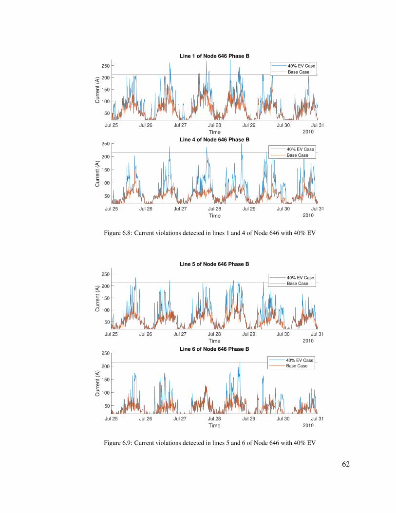
Jul 25 Jul 26 Jul 27 Jul 28 Jul 29 Jul 30 Jul 31
Time 2010
50
100
150
200
250
Curr
ent (A
)
Line 1 of Node 646 Phase B
40% EV Case
Base Case
Jul 25 Jul 26 Jul 27 Jul 28 Jul 29 Jul 30 Jul 31
Time 2010
50
100
150
200
250
Curr
ent (A
)
Line 4 of Node 646 Phase B
40% EV Case
Base Case
Figure 6.8: Current violations detected in lines 1 and 4 of Node 646 with 40% EV
Jul 25 Jul 26 Jul 27 Jul 28 Jul 29 Jul 30 Jul 31
Time 2010
50
100
150
200
250
Cu
rren
t (A
)
Line 5 of Node 646 Phase B
40% EV Case
Base Case
Jul 25 Jul 26 Jul 27 Jul 28 Jul 29 Jul 30 Jul 31
Time 2010
50
100
150
200
250
Cu
rre
nt (A
)
Line 6 of Node 646 Phase B
40% EV Case
Base Case
Figure 6.9: Current violations detected in lines 5 and 6 of Node 646 with 40% EV
62

As the penetration of EV level increases, more current violation events are recorded by
the Current Violation tool. At 60% EV penetration, several events are detected. Figures 6.10
and 6.11 show the current violation events for four lines. These results illustrate that at 60%
EV penetration, most of the lines have current violations. These occur for about 20 minutes
maximum. As a result, appropriate action could be recommended to resize conductors to
avoid overheating conditions, which may exist due to the anticipated load growth.
Jul 25 Jul 26 Jul 27 Jul 28 Jul 29 Jul 30 Jul 31
Time 2010
50
100
150
200
250
Curr
ent (A
)
Line 1 of Node 646 Phase B
60% EV Case
Base Case
Jul 25 Jul 26 Jul 27 Jul 28 Jul 29 Jul 30 Jul 31
Time 2010
50
100
150
200
250
Curr
ent (A
)
Line 4 of Node 646 Phase B
60% EV Case
Base Case
Figure 6.10: Current violations detected in lines 1 and 4 of Node 646 with 60% EV
63

Jul 25 Jul 26 Jul 27 Jul 28 Jul 29 Jul 30 Jul 31
Time 2010
100
200
300
Cu
rre
nt
(A)
Line 7 of Node 646 Phase B
60% EV Case
Base Case
Jul 25 Jul 26 Jul 27 Jul 28 Jul 29 Jul 30 Jul 31
Time 2010
0
100
200
300
Cu
rre
nt
(A)
Line 8 of Node 646 Phase B
60% EV Case
Base Case
Figure 6.11: Current violations detected in lines 7 and 8 of Node 646 with 60% EV
Furthermore, at node 646 phase B with 80% EV penetration, six out of eight lines were
found to have current violations. About 75% of the total lines are experiencing current
violations issue. Figures 6.12 - 6.14 show these events within the affected lines. From the
simulated results, Line 8 experienced the lonest duration of current violation events, for
about 30 minutes. The maximum simulated current value was 296 A, which is about 138%
of the ampacity capacity value.
64

Jul 25 Jul 26 Jul 27 Jul 28 Jul 29 Jul 30 Jul 31
Time 2010
100
200
300
Curr
ent (A
)
Line 1 of Node 646 Phase B
80% EV Case
Base Case
Jul 25 Jul 26 Jul 27 Jul 28 Jul 29 Jul 30 Jul 31
Time 2010
0
100
200
300
Curr
ent (A
)
Line 4 of Node 646 Phase B
80% EV Case
Base Case
Figure 6.12: Current violations detected in lines 1 and 4 of Node 646 with 80% EV
Jul 25 Jul 26 Jul 27 Jul 28 Jul 29 Jul 30 Jul 31
Time 2010
50
100
150
200
250
Cu
rre
nt
(A)
Line 5 of Node 646 Phase B
80% EV Case
Base Case
Jul 25 Jul 26 Jul 27 Jul 28 Jul 29 Jul 30 Jul 31
Time 2010
0
50
100
150
200
250
Cu
rre
nt
(A)
Line 6 of Node 646 Phase B
80% EV Case
Base Case
Figure 6.13: Current violations detected in lines 5 and 6 of Node 646 with 80% EV
65

Jul 25 Jul 26 Jul 27 Jul 28 Jul 29 Jul 30 Jul 31
Time 2010
0
100
200
300
Curr
ent (A
)
Line 7 of Node 646 Phase B
80% EV Case
Base Case
Jul 25 Jul 26 Jul 27 Jul 28 Jul 29 Jul 30 Jul 31
Time 2010
0
100
200
300
Curr
ent (A
)
Line 8 of Node 646 Phase B
80% EV Case
Base Case
Figure 6.14: Current violations detected in lines 7 and 8 of Node 646 with 80% EV
The Current Violation tool results with the simulation test cases showed that as EV
penetration level increases, so do the number and duration of current violation events at the
distribution overhead lines examined on the IEEE 13 node test feeder as presented using
node 646. The occurrence of current violations on the overhead conductors poses a major
issue in distribution system infrastructure assets. To maintain grid reliability and customer
safety, the current should be at or below the rated conductor ampacity. When the conductor
current exceeds the ampacity value, the conductor will overheat, leading to decrease asset
lifetime, power loss, and excessive voltage drops. Consequently, evaluating the impact of
projected EV load growth is essential for preparing distribution system to provide service
to EV owners. The Current Violation tool is a simple means to analyze and detect current
violations events using simulation data.
66

6.2 Winter EV Test Case
The Winter EV Test case uses the winter load profiles. These represent typical energy
consumption for the mid-western United States and run for a period of one week. The
Winter EV Test case was considered to analyze the impact of EV load growth and to present
tool evaluation comparison with winter energy use. While developing the Winter EV Test
case, three conditions were considered. First, a test case was developed for examining
transformer overloading events. Second, penetration levels of EV ranging from 20% to
100% were examined. Test cases focused on three-phase nodes of the IEEE 13 node test
feeder model. In the following sections, an illustration of the test results are demonstrated to
support the major of the analysis.
6.2.1 Transformer Overloading Tool
For the Winter EV Test case, node 692 was chosen from the IEEE 13 node test feeder model
to test the Transformer Overloading tool. Node 692 is a three-phase node. Seven distribution
transformers are attached to each phase. Distribution transformers are rated between 15 - 35
kVA, at increments of 5 kVA. For this case analysis, EV loads were added gradually by 20%
for each simulation test.
The Transformer Overloading tool was applied to the IEEE 13 node test feeder model.
This test case applied to phase A,B and C of node 692. Phase A of node 692 is connected to
seven transformers and serve total of 38 household.
67

At 20% EV penetration, results showed no transformer overloading events. However, at
40% the Transformer Overloading tool detected events occurred for 30 minutes and an hour.
Additional events were examined at 60% EV penetration. Four distribution transformers
were overloaded for two hours, six overloading events were detected for an hour, and 16
transformer overloading events were detected for 30 minutes. In summary, higher EV
penetration leads to a greater number of duration overloading events. To better identify
distribution transformer overloading events, histograms are examined. Figure 6.15 represent
histograms plot of node 692 A. These histograms highlight the duration of transformer
overloading events and the occurrence for each duration. Histograms presented in Figure
6.15 show the duration of 30 minutes to four hours events. However, 30 minutes overloading
events are not of concern, due to the short period of these events. Events were examined to
the reference of ANSI and IEEE standard [4]. Therefore, one-half hour events can deliver
200% load of the nameplate rate without damaging the transformer.
Figure 6.15: Transformer overloading events histograms at Node 692 phase A
68

The same testing procedures applied to phase A of node 692 are used to phase B, and
C. A total of 114 households are attached to node 692, in which 38, 35 and 41 houses are
connected to phase A, B, and C, respectively. Histograms of transformer overloading events
of phase B and C show that with large EV penetrations have more overloading events and
for longer duration, as shown in Figures 6.16 and 6.17. Test results lead to the conclusion
that the impact of EV load growth on distribution transformer overloading events gradually
increase as the EV penetration increases.
Figure 6.16: Transformer overloading events histograms at Node 692 phase B
Figure 6.17: Transformer overloading events histograms at Node 692 phase C
69

7 Conclusion
This thesis motivation was to develop tools for analyzing the impacts of projected EV
load growth. A suite of tools was successfully developed to model the impact of EV
loads on power distribution infrastructure assets. These tools indicate voltage violations
within a distribution network, detect over-current violation events associated with overhead
conductors, and reveal distribution transformer overload events. These tools were developed
for use in GridLAB-D and written using Python 3.8. Such tools can be used to help utility
distribution planners prepare appropriate responses for the anticipated EV load growth.
When EV load growth increases, power distribution lines and transformers are impacted.
The tools developed for this thesis showed evidence that at only 40% - 60% penetration,
distribution transformers become overloaded, distribution lines experience voltage violation
events, and conductors exceed the rated ampacity. Thus, planner engineers can use these
tools to study and analyze EV load growth impact and then take appropriate actions.
Several opportunities for future improvement are possible to enhance analyzing EV
load growth impact on power distribution infrastructure assets. One possible improvement
is to use Hierarchical Engine for Large-scale Infrastructure Co-Simulation (HELICS) to
enable bringing together multiple existing software tools. For example, one could develop
distribution feeder in GridLAB-D and then integrated with Python or a C++ compiler to
control the tool during simulation. Another possible opportunity is to simulate DCFC. This
70

improvement would help utilities to examine the commercial side of their assets particularly
high-power EV chargers. A final improvement opportunity would be developing a tool that
examines the impact of the harmonic distortion in the conductors. However, GridLAB-D
may not be the optimal platform for such analysis.
71

Bibliography
[1] Office of Transportation and Air Quality. Fast Facts: U.S. Transportation Sector
Greenhouse Gas Emissions 1990-2018. June 2020.
[2] Cambridge University Press. Climate Change 2014 Mitigation of Climate Change .
January 2014.
[3] Transportation Electrification Plan. Portland General Electric, March 2017.
[4] IEEE guide for loading dry-type distribution and power transformers. IEEE Std
C57.96-1999, pages 1–48, 2014.
[5] ANSI C84.1 Power Systems and Equipment – Voltage Ratings (60 Hz). National
Electrical Manufacturers Association, 2006.
[6] D. P. Chassin, K. Schneider, and C. Gerkensmeyer. GridLAB-D: An open-source
power systems modeling and simulation environment. In 2008 IEEE/PES Transmission
and Distribution Conference and Exposition, pages 1–5, 2008.
[7] M. A. Al Faruque and F. Ahourai. Modeling and simulation of the EV charging in
a residential distribution power grid. In Proceedings of Green Energy and Systems
Conference 2013, pages 1–4, 2013.
72

[8] D. Wang, B. de Wit, S. Parkinson, J. Fuller, D. Chassin, C. Crawford, and N. Djilali. A
test bed for self-regulating distribution systems: Modeling integrated renewable energy
and demand response in the GridLAB-D/MATLAB environment. In 2012 IEEE PES
Innovative Smart Grid Technologies (ISGT), pages 1–7, 2012.
[9] M. Moffet, F. Sirois, and D. Beauvais. Review of Open Source Code Power Grid
Simulation. Technical report, Canmet ENERGY, Natural Resources Canada, 2011.
[10] S. Shao, M. Pipattanasomporn, and S. Rahman. Challenges of PHEV penetration to
the residential distribution network. In 2009 IEEE Power Energy Society General
Meeting, pages 1–8, 2009.
[11] A. Hilshey, P. Hines, P. Rezai, and J. Dowds. Estimating the impact of electric vehicle
smart charging on distribution transformer aging. In 2013 IEEE Power Energy Society
General Meeting, pages 1–1, 2013.
[12] A. Dubey, S. Santoso, and M. P. Cloud. Understanding the effects of electric vehicle
charging on the distribution voltages. In 2013 IEEE Power Energy Society General
Meeting, pages 1–5, 2013.
[13] J. Taylor, A. Maitra, M. Alexander, D. Brooks, and M. Duvall. Evaluation of the
impact of plug-in electric vehicle loading on distribution system operations. In 2009
IEEE Power Energy Society General Meeting, pages 1–6, 2009.
73

[14] A. Ul-Haq, A. Perwaiz, M. Azhar, and S. Ullah Awan. Harmonic distortion in distribu-
tion system due to single-phase electric vehicle charging. In 2018 2nd International
Conference on Green Energy and Applications (ICGEA), pages 205–209, 2018.
[15] N. Woodman, R. B. Bass, and M. Donnelly. Modeling harmonic impacts of electric
vehicle chargers on distribution networks. In 2018 IEEE Energy Conversion Congress
and Exposition (ECCE), pages 2774–2781, 2018.
[16] W. H. Kersting. Radial distribution test feeders. In 2001 IEEE Power Engineering
Society Winter Meeting. Conference Proceedings (Cat. No.01CH37194), volume 2,
pages 908–912 vol.2, 2001.
[17] Alomani Shahad. Data from: Power distribution system tools for analyzing impacts
of projected Electric Vehicle load growth using GridLab-D, 2021. Electrical and
Computer Engineering Datasets.1, https://doi.org/10.15760/ece-data.
01.
[18] Pacific Northwest National Laboratory. Gridlab-D Technical Support Document: Tape
Modules Version 1.0. May 2008.
[19] W. H. Kersting. Distribution System Modeling and Analysis, 2nd Edition. CRC Press,
2007.
[20] Pacific Northwest National Laboratory. Power Flow User Guide. April 2010.
http://gridlab-d.shoutwiki.com/wiki/Power_Flow_User_Guide.
74

[21] F. Ahourai and M. A. Al Faruque. Grid Impact analysis of a Residential Microgrid
under various EV penetration rates in GridLAB-D. Technical report, University of
California, 2013.
[22] Matteo Muratori. Impact of uncoordinated plug-in electric vehicle charging on resi-
dential power demand. Nature Energy, 3:193, March 2018.
[23] C. Berry. Residential Energy Consumption Survey (RECS). U.S. Energy Information
Administration, April 2016.
[24] Matteo Muratori, Michael J. Moran, Emmanuele Serra, and Giorgio Rizzoni. Highly-
resolved modeling of personal transportation energy consumption in the United States.
Energy, 58(C):168–177, 2013.
[25] NFPA 70: National Electrical Code Second Revision, Copyright, National Fire Protec-
tion Association. 2015.
75

Appendix A: Tables
A.1 Transformers and houses distributed along IEEE 13 node test feeder
A.1.1 Single phase node
IEEE 13 Nodes Phase Transformer Rating ( kVA) Number of Houses
Node 652 A
35 735 730 635 730 620 435 715 3
IEEE 13 Nodes Phase Transformer Rating ( kVA) Number of Houses
Node 645
B
15 525 325 415 615 725 520 435 5
C
30 625 525 535 715 335 720 430 6
76

A.1.2 Two phase nodes
IEEE 13 Nodes Phase Transformer Rating ( kVA) Number of Houses
Node 684
A
30 635 730 635 720 415 335 730 6
C
15 335 715 325 515 315 320 4
IEEE 13 Nodes Phase Transformer Rating ( kVA) Number of Houses
Node 646
B
25 515 320 430 630 620 415 315 3
C
20 435 730 615 330 635 725 525 5
77

A.1.3 Three phase nodes
IEEE 13 Nodes Phase Transformer Rating ( kVA) Number of Houses
Node 632
A
20 435 715 320 430 625 535 720 4
B
25 535 725 535 725 535 720 435 7
C
25 530 615 325 520 435 730 630 6
IEEE 13 Nodes Phase Transformer Rating ( kVA) Number of Houses
Node 692
A
15 330 625 530 635 725 530 6
B
25 515 330 630 615 330 630 6
C
20 425 535 735 735 735 720 4
78

IEEE 13 Nodes Phase Transformer Rating ( kVA) Number of Houses
Node 675
A
25 525 530 630 615 335 725 5
B
25 525 530 625 530 630 630 6
C
35 715 320 430 620 415 330 6
IEEE 13 Nodes Phase Transformer Rating ( kVA) Number of Houses
Node 671
A
20 435 715 325 535 720 420 4
B
25 520 430 635 735 720 420 425 5
C
30 625 515 330 635 725 535 7
79

IEEE 13 Nodes Phase Transformer Rating ( kVA) Number of Houses
Node 680
A
35 715 330 615 330 630 620 4
B
30 615 330 630 620 420 430 630 6
C
30 635 720 425 530 620 420 4
80

A.2 Python Code
A.2.1 Voltage Violation Tool
## This code is for checking Voltage Violations with ANSI C84.1
standard:
## [114V] ---- [120V] ---- [126V] +/-5%
## Ask the user which standard?
## Input file >> CSV of Timestamp and Simulated measured voltage
## Output >> Voltage Violations Events, If no Voltage Violations
detected, No # WARNING:
import pandas as pd
import numpy as np
def ansic84():
'''
handles ansic84
'''
ideal = minLimit = maxLimit = 120
maxLimit += ideal * 0.05
minLimit -= ideal * 0.05
dev = {}
f = input("enter file name: ")
try:
81

csv =
pd.read_csv(f,skiprows=range(0,7),error_bad_lines=False)
csv.rename({'#
timestamp':'timestamp'},axis='columns',inplace=True)
# change values
for i in csv.columns[1:]:
csv[i] = csv[i].str.replace('d','j')
csv[i] = csv[i].apply(lambda x:np.complex(x).real)
csv[i] = pd.to_numeric(csv[i])
dev[i+'_min'] = csv[csv[i]<=minLimit] # check for values
below minLimit
dev[i+'_max'] = csv[csv[i]>=maxLimit] # check for values
above maxLimit
if dev[i+'_min'].empty:
dev[i+'_min'] = 'NO WARNING'
if dev[i+'_max'].empty:
dev[i+'_max'] = 'NO WARNING'
# print( dev[i+'_max'])
for k,v in dev.items():
print(f'{"-"*20}{k}{"-"*20}')
print(v)
print(f"ideal: {ideal} ; max: {maxLimit} ; min: {minLimit}")
except Exception as e:
82

print(e)
print("-"*5+">Error occured\nexiting...")
exit()
return
def main():
stds = {1:'ANSIC84'}
funcs = {'ANSIC84':ansic84}
print("enter your desired standard:")
std = int(input("[1] - ANSI C84\n[2] - XX\n"))
if not std in stds:
print("-"*5+">Not a supported standard\nexiting...")
exit()
print(f"you entered {std} : {stds[std]}")
'''
call ansi
'''
std = stds[std]
funcs[std]()
if __name__=="__main__":
main()
exit()
83

A.2.2 Current Violation Tool
## This code is for checking Current Violations of Overhead
conductors
## Input Files : >> CSV of Timestamp and Simulated measured
current
## Output >> Current Violations Events, Current exceeded amapcity
rating and % of Violations
'''
*** THIS FILE NEEDS TO BE IN A DIRECTORY WITH ONLY THE FILES
TO BE PARSED ***
'''
import pandas as pd
import numpy as np
import os
DIR = '.' # directory where csv files are stored
VALUE = # value to check against for values greater than
output_file = 'output.csv'
outs = {}
files = os.listdir(DIR)
files = filter(lambda x: x.endswith('.csv'),files)
def convert_complex(c):
84

x = c.real
y = c.imag
return np.sqrt(x*x+y*y)
def fun(value):
percentage = (value/VALUE) *100
return f'{round(percentage,3)}%'
for f in files:
try:
csv = pd.read_csv(f,skiprows=range(0,7))
csv.set_index(csv.columns[0],inplace=True)
for col_name in csv.columns[1:]:
col = csv[col_name].str.replace('d','j').str.replace('
','').apply(lambda x:
np.complex(x)).rename('complex')
converted = col.apply(lambda x:
convert_complex(x)).rename('converted')
percentage = converted.apply(lambda x:
fun(x)).rename('percentages')
df = pd.concat([col,converted,percentage],axis=1)
df = df[df['converted'] >= VALUE]
outs[col_name] = df
except Exception as e:
85

print(e)
with open(output_file,'w') as f:
for k,v in outs.items():
f.write(f"{'-'*20} {k} {'-'*20}\n")
f.write(v.to_csv())
86

A.2.3 Transformer Overloading Tool
'''
## This code is for checking Overloading transfomers conditions
## Input Files : >> CSV of Timestamp and Simulated measured Power
## Output >> Overloaded Transformers depend on % of Overloaded
condition provided with the duration of Overloading
'''
import pandas as pd
import argparse
import time
import numpy as np
import os
def get_power_rates(cols):
power_rates = []
# compare against the given Y value
for i in cols:
power_rates.append(float(input(f"enter {i} Power Rate: ")))
return power_rates
def get_file_names():
files = []
for c in cols:
files.append(input(f"enter name of output file for {c}: "))
87

return files
def query_csv():
vals = []
for y,c in zip(power_rates,cols):
vals.append(csv.query(f"`{c}` >= {y}"))
return vals
def first_version():
'''
first verison just writes the query results to their
respective files
'''
for v,f,c in zip(query_results,output_files,cols):
v[["# timestamp",f"{c}"]].to_csv(f"{f}",index=False)
return
def query(df, col, t_delta, ep, pr,step):
sz = csv.shape[0]
res = []
result = []
df = csv[['# timestamp',col,'timestamp']] # change from csv to
df
i = 0
steps = pd.Timedelta(step,unit='m')
if i<sz:
88

prev = df.loc[0]
while i < sz:
cur = df.loc[i]
if cur['timestamp'] == (prev['timestamp'] + steps) and
(abs(cur[col] - pr) <= ep) and (abs(prev[col] - pr) <=
ep):
res.append(prev)
if t_delta/step == len(res):
res.append(cur)
result.append(res)
res = []
else:
res = []
prev = cur
i += 1
return result
def open_file(FILE):
csv = pd.read_csv(FILE)
cols = csv.columns[1:]
csv['timestamp'] = pd.to_datetime(csv['# timestamp']) #
convert normal timestamp format to datetime timestamp
csv['timestamp'].apply(lambda x: time.mktime(x.timetuple())) #
converts datetime timestamp to unix timestamp
89

return (csv,cols)
def second_version(csv):
'''
200% ----------------- 30 minutes
150% ----------------- 1 hour
125% ----------------- 4 hours
others ----------------- remaining
second version checks for time constraints before writing the
query results to their respective files
'''
specs = {} # these specs define the previously stated rules
# query for the 1.25 === %125
# there will be only 1 column (besides timestamps) & 1
power_rate for the column
pr = power_rates[0]
col = cols[0]
# ------------- 200% -------------
x = 2 * pr
# 10% of x
ep = 0.1 * x
print(f"{50*'-'} calculating 200% {50*'-'}")
res = query(csv,col,30 ,ep,x, 10) # 30 minutes and 10 minutes
step ( in case that changes in the future)
90

if len(res) > 0:
res = sum(res,[])
df = pd.DataFrame(res)
print(df)
specs[f"#{50*'-'} {FILE}--(200%) {50*'-'}"] = df
# ------------- 150% -------------
x = 1.5 * pr
# 10% of x
ep = 0.1 * x
print(f"{50*'-'} calculating 150% {50*'-'}")
res = query(csv,col,60 ,ep,x, 10) # 60 minutes and 10 minutes
step ( in case that changes in the future)
if len(res) > 0:
res = sum(res,[])
df = pd.DataFrame(res)
print(df)
specs[f"#{50*'-'} {FILE}--(150%) {50*'-'}"] = df
# ------------- 125% -------------
x = 1.25 * pr
# 10% of x
ep = 0.1 * x
print(f"{50*'-'} calculating 125% {50*'-'}")
91

res = query(csv,col,240 ,ep,x, 10) # 240 minutes and 10
minutes step ( in case that changes in the future)
if len(res) > 0:
res = sum(res,[])
df = pd.DataFrame(res)
print(df)
specs[f"#{50*'-'} {FILE}--(125%) {50*'-'}"] = df
return specs
def write_output(fname,output):
if os.path.exists(fname):
os.remove(fname)
for DICT in output:
if DICT:
for k,v in DICT.items():
with open(fname,'a+') as f:
f.write(k+'\n')
del v['timestamp']
v.to_csv(fname,mode='a',index=False)
return
parser = argparse.ArgumentParser(description='.')
parser.add_argument('-f', type=str, help='input file
name',default='')
92
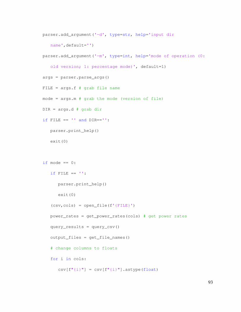
parser.add_argument('-d', type=str, help='input dir
name',default='')
parser.add_argument('-m', type=int, help='mode of operation (0:
old version; 1: percentage mode)', default=1)
args = parser.parse_args()
FILE = args.f # grab file name
mode = args.m # grab the mode (version of file)
DIR = args.d # grab dir
if FILE == '' and DIR=='':
parser.print_help()
exit(0)
if mode == 0:
if FILE == '':
parser.print_help()
exit(0)
(csv,cols) = open_file(f'{FILE}')
power_rates = get_power_rates(cols) # get power rates
query_results = query_csv()
output_files = get_file_names()
# change columns to floats
for i in cols:
csv[f"{i}"] = csv[f"{i}"].astype(float)
93

first_version()
elif mode == 1:
output = []
if DIR == '':
parser.print_help()
exit(0)
# read all files in the given directory
if DIR[-1] != '/':
DIR += '/'
for FILE in os.listdir(DIR):
print(f"{'*'*50} {FILE} {'*'*50}")
(csv,cols) = open_file(f'{DIR}{FILE}')
power_rates = get_power_rates(cols) # get power rates
res = second_version(csv)
output.append(res)
write_output('output.csv',output)
# second_version()
94

A.3 IEEE 13 Node Test Feeder Model in GridLAB-D
A.3.1 Input Data Files
Season Load profile
SummerHouseholdsHouseholds + EV
WinterHouseholdsHouseholds + EV
A.3.2 Glm Files
Summer CasesCases Cases information
Summer Base Case Base case GridLab-D model configuration with no EV20% EV Case EV case with 200 EVs40% EV Case EV case with 400 EVs60% EV Case EV case with 600 EVs80% EV Case EV case with 800 EVs
100% EV Case EV case with 1000 EVs
Winter CasesCases Cases information
Winter Base Case Base case GridLab-D model configuration with no EV20% EV Case EV case with 200 EVs40% EV Case EV case with 400 EVs60% EV Case EV case with 600 EVs80% EV Case EV case with 800 EVs
100% EV Case EV case with 1000 EVs
95