power control in integrated access and backhaul networks
TRANSCRIPT

Power Control in Integrated Access andBackhaul NetworksMaster’s thesis in Communication Engineering
Haitham BabbiliOlalekan Peter Adare
DEPARTMENT OF ELECTRICAL ENGINEERING
CHALMERS UNIVERSITY OF TECHNOLOGYGothenburg, Sweden 2021www.chalmers.se


Master’s thesis 2021
Power Control in Integrated Access and BackhaulNetworks
Haitham BabbiliOlalekan Peter Adare
Department of Electrical EngineeringWireless Systems Division
Communication Systems GroupChalmers University of Technology
Gothenburg, Sweden 2021

Power Control in Integrated Access and Backhaul NetworksHAITHAM BABBILI, OLALEKAN PETER ADARE
© Haitham Babbili, 2021.© Olalekan Peter Adare, 2021.
Supervisor: Tommy Svensson, Department of Electrical Engineering, Chalmers
Co-supervisor(s):Behrooz Makki, Ericsson ResearchCharitha Madapatha, Department of Electrical Engineering, Chalmers
Examiner: Tommy Svensson, Department of Electrical Engineering, Chalmers
Master’s Thesis 2021Department of Electrical EngineeringWireless Systems DivisionCommunication Systems GroupChalmers University of TechnologySE-412 96 GothenburgTelephone +46 31 772 1000
Cover: Illustration of an integrated access and backhaul network in urban macroenvironment.
Typeset in LATEX, template by Magnus GustaverPrinted by Chalmers ReproserviceGothenburg, Sweden 2021
iv

Power Control in Integrated Access and Backhaul NetworksHAITHAM BABBILI, OLALEKAN PETER ADAREDepartment of Electrical EngineeringChalmers University of Technology
AbstractThe integrated access and backhaul (IAB) network is a novel radio access network(RAN) solution, proposed by the 3rd Generation Partnership Project (3GPP). IABnetwork is one of the interesting aspects of the fifth-generation (5G) RAN. The IABnetworks thrives on the advantage of using all ranges of spectrum defined for the 5Gnew radio (NR) to interconnect the mobile and fixed access users to the network,and still bulk transmit their data towards the 5G core network. IAB networks mayreduce the dependency on the optical fiber network and out-of-band frequencies forbackhauling. However, there are inherent challenges that come with this approach.A possible constraint may be interference, which reduces the received signal quality.This, in turn, reduces the user data rate. Therefore, interference should be mitigatedor canceled optimally. Using power control combined with adaptive beamforming,resource allocation and routing techniques may help to deploy efficient IAB networks,with higher spectral efficiency and better service coverage.This thesis focuses on a power control solution in uplink communication within IABnetworks. A power control solution may effectively reduce the effects of interferenceamong all the transceivers and keep the network operating at a signal-to-interference-plus-noise-ratio (SINR) that is needed to guarantee mobile services. The solutionis built on a genetic algorithm (GA), which offers reasonable solutions in multi-objective problem formulations. The performance of the solution is then evaluatedusing the service coverage probability. Service coverage probability is the probabilityof the event that the users are provided with a minimum data rate. First, a wirelessnetwork model is set-up using using millimeter wave characteristics. Then, a finitecoverage area is built with randomly distributed users and statically positionedbase stations with transmit power constraints, as proposed by 3GPP. Afterwards, awireless access channel is modeled that takes into account the predominant channelconstraints, where the duplexing mode is time division duplex (TDD). Finally, theSINR and transmit power of all mobile terminals (MT) are optimized at every epochusing the GA. Interestingly, the GA offers a proper convergent solution for powercontrol in IAB networks. Furthermore, based on the various simulations and results,there is a possibility that IAB networks with a well implemented power controlscheme can achieve a better service coverage probability in uplink communication,than non-IAB networks.
Keywords: 5G NR, Integrated access and backhaul, IAB, signal-to-interference-plus-noise-ratio, 3GPP, power control, uplink, service coverage probability, geneticalgorithm, wireless backhaul.
v


AcknowledgementsFirst of all, our profound gratitude goes to Professor Tommy Svensson for giving usthis rare opportunity to conduct the thesis. He offered his plethora of knowledgein supervising our work. He offered us a high degree of academic research freedomwhich enabled us to learn and re-learn satisfactorily. Your always friendly and pro-fessional approach is endearing. Without your help, the aim of the project wouldnot have been actualized.
Secondly, we are indebted to Dr. Behrooz Makki from Ericsson. He was alwaysavailable and down to earth in offering guidance from his wealth of experience onthe practical solutions in 5G networks and beyond. You were motivating us con-sistently while offering words of advice at each stage. It would have been difficultto get this done without you. We thank you. Our deepest appreciation goes toEricsson AB for their overall support and technical guidance. Concisely, withoutyou offering this thesis work, we would not have seen the bigger picture and thevarious solutions that abound in the telecommunication industry.
Thirdly, we wish to show our gratitude to Charitha Madapatha. He was our co-supervisor and his earlier work on 5G and beyond complemented our project. Yoursimplified explanations, information, guidance and support were a huge advantagefor us.
Furthermore, our sincere thanks go to the department of Electrical engineering, atChalmers University of Technology. You made us see the engineering world froma unique prism of life. The enabling environment, opportunities and the generalknowledge offered are top-notch.
Then, we would like to recognize the irreplaceable help from our families during ourstudy. Your encouragement and resolute support gave us the needed strength tocarry on. Without you, we would not have achieved a lot of our goals. We sincerelyappreciate you.
Haitham Babbili and Olalekan Peter Adare, Gothenburg, June 2021
vii


List of AcronymsBS Base StationsCSI Channel State InformationCU Central UnitDL DownlinkDU Distributed UniteMBB Enhanced Mobile BroadbandFDD Frequency Division DuplexFHPPP Finite Homogeneous Poisson Point ProcessFWA Fixed Wireless AccessGA Genetic AlgorithmgNB Next Generation NodeBHARQ Hybrid Automatic Repeat RequestHetNet Heterogeneous NetworkIAB Integrated Access and BackhaulITU-R International Telecommunication Union-Radio communication sectorKPI Key Performance IndicatorLOS Line-of-SightLTE Long Term EvolutionmMTC Massive Machine-type CommunicationMBS Macro Base StationMIMO Multiple-Input-Multiple-OutputmmWave Millimeter WaveNLOS Non-Line-of-SightNR New RadioOFDM Orthogonal Frequency Division MultiplexingQAM Quadrature Amplitude ModulationQoE Quality of ExperienceQoS Quality of ServiceRAN Radio Access NetworkRAT Radio Access TechnologyRB Resource BlockSBS Small Base StationSDM Space Division MultiplexingSINR Signal-to-Interference-plus-Noise RatioTDD Time Division DuplexUE User EquipmentUMa Urban MacroUL UplinkuRLLC Ultra Reliable Low Latency CommunicationVR Virtual RealityWDM Wavelength Division MultiplexingWi-Fi Wireless FidelityWiMAX Worldwide Interoperability for Microwave Access2G Second Generation
ix

3G Third Generation3GPP 3rd Generation Partnership Project4G Fourth Generation5G Fifth Generation
x


Contents
List of Figures xv
List of Tables xix
1 Introduction 11.1 Background and Motivation . . . . . . . . . . . . . . . . . . . . . . . 11.2 Aim . . . . . . . . . . . . . . . . . . . . . . . . . . . . . . . . . . . . 31.3 Thesis Contribution . . . . . . . . . . . . . . . . . . . . . . . . . . . . 31.4 Limitations . . . . . . . . . . . . . . . . . . . . . . . . . . . . . . . . 31.5 Methodology . . . . . . . . . . . . . . . . . . . . . . . . . . . . . . . 31.6 Previous Work . . . . . . . . . . . . . . . . . . . . . . . . . . . . . . 41.7 Thesis Outline . . . . . . . . . . . . . . . . . . . . . . . . . . . . . . . 5
2 Theoretical Background 62.1 5G New Radio . . . . . . . . . . . . . . . . . . . . . . . . . . . . . . . 62.2 5G IAB Network Structure . . . . . . . . . . . . . . . . . . . . . . . . 82.3 Structure of IAB Nodes . . . . . . . . . . . . . . . . . . . . . . . . . 122.4 The Role of Power Control in IAB Networks . . . . . . . . . . . . . . 12
3 System Model 143.1 Model Set-up . . . . . . . . . . . . . . . . . . . . . . . . . . . . . . . 143.2 Channel Modelling . . . . . . . . . . . . . . . . . . . . . . . . . . . . 16
3.2.1 Received Power . . . . . . . . . . . . . . . . . . . . . . . . . . 163.2.2 Pathloss and Shadowing . . . . . . . . . . . . . . . . . . . . . 163.2.3 Rain Effect . . . . . . . . . . . . . . . . . . . . . . . . . . . . 173.2.4 Fading Effect . . . . . . . . . . . . . . . . . . . . . . . . . . . 183.2.5 Total Channel Loss . . . . . . . . . . . . . . . . . . . . . . . . 18
3.3 Interference . . . . . . . . . . . . . . . . . . . . . . . . . . . . . . . . 183.4 SINR and Baseline SINR Value . . . . . . . . . . . . . . . . . . . . . 183.5 Receiver Sensitivity . . . . . . . . . . . . . . . . . . . . . . . . . . . . 193.6 Resource Block . . . . . . . . . . . . . . . . . . . . . . . . . . . . . . 193.7 UE and SBS Association . . . . . . . . . . . . . . . . . . . . . . . . . 193.8 Service Coverage Probability . . . . . . . . . . . . . . . . . . . . . . . 203.9 Achievable Data Rate of the UE . . . . . . . . . . . . . . . . . . . . . 203.10 Access and Backhaul Bandwidth Utilization . . . . . . . . . . . . . . 203.11 TDD Scheduler for MBS/SBS/UE . . . . . . . . . . . . . . . . . . . . 213.12 Genetic Algorithm for Power Control . . . . . . . . . . . . . . . . . . 23
xii

Contents
4 Simulation and Results 254.1 Effect of Rain . . . . . . . . . . . . . . . . . . . . . . . . . . . . . . . 264.2 Effect of Increase in RB per UE and Power Control (One Cell) . . . . 274.3 Effect of Increase in RB per UE and Power Control (Two Cells) . . . 304.4 Effect of Interference on Simultaneous Access and Backhaul Links
(One Cell) . . . . . . . . . . . . . . . . . . . . . . . . . . . . . . . . . 334.5 Effect of Interference on Simultaneous Access and Backhaul Links
(Two Cells) . . . . . . . . . . . . . . . . . . . . . . . . . . . . . . . . 364.6 Data Rate Analysis for the UEs . . . . . . . . . . . . . . . . . . . . . 394.7 Comparison between IAB and non-IAB Network . . . . . . . . . . . . 424.8 Determination of the Effective Cell Radius . . . . . . . . . . . . . . . 434.9 Transmit Power Distribution of UEs . . . . . . . . . . . . . . . . . . 444.10 Convergence of the Genetic Algorithm . . . . . . . . . . . . . . . . . 46
5 Conclusion 48
6 Future Works 49
Bibliography 51
A Appendix 1 IA.1 Inter-cell Distance and Inter-cell Interference . . . . . . . . . . . . . . IA.2 Intra-cell Distance and Intra-cell Interference . . . . . . . . . . . . . . I
xiii

Contents
xiv

List of Figures
2.1 Illustration of 5G NR use cases. 5G NR services are classified aseMMB, URLLC and mMTC. . . . . . . . . . . . . . . . . . . . . . . 6
2.2 Illustration of FDD and TDD. Duplexing is based on time-frequencyallocation for UL and DL. . . . . . . . . . . . . . . . . . . . . . . . . 9
2.3 Illustration of UL and DL Communication. The BS is taken as areference point for UL/DL illustration. . . . . . . . . . . . . . . . . . 9
2.4 Illustration of 5G IAB network. There is one central MBS and fourother SBSs depend on it for backhauling. . . . . . . . . . . . . . . . . 10
2.5 Resource sharing between MBS, SBS and UE. From [29]. Reproducedwith permission. . . . . . . . . . . . . . . . . . . . . . . . . . . . . . . 12
2.6 The Architecture of SBS/IAB nodes. . . . . . . . . . . . . . . . . . . 13
3.1 Schematic diagram of the system model of an IAB network. . . . . . 143.2 Illustration of d2D and d3D distances. From [33]. Reproduced with
permission. . . . . . . . . . . . . . . . . . . . . . . . . . . . . . . . . 173.3 First TDD Epoch. Here, only SBSs are transmitting within the cell. . 213.4 Second TDD Epoch. Here, only the UEs are transmitting within the
cell. . . . . . . . . . . . . . . . . . . . . . . . . . . . . . . . . . . . . 223.5 Special TDD case. Here, only the SBSs and the UEs associated with
the MBS are transmitting. . . . . . . . . . . . . . . . . . . . . . . . . 22
4.1 ITU-RP.838-3 rain loss for 28 GHz for varying rain rates up to 120mm/h (r = 200 m, fc = 28 GHz). . . . . . . . . . . . . . . . . . . . . 26
4.2 2D illustration of 1 MBS single-cell with MATLAB. . . . . . . . . . . 274.3 One cell: Service coverage probability versus the number of UEs with
1 RB per UE (r = 200 m, M = 4, E = 65). . . . . . . . . . . . . . . 284.4 One cell: Service coverage probability versus the number of UEs with
2 RBs per UE (r = 200 m, M = 4, E = 65). . . . . . . . . . . . . . . 284.5 One cell: Service coverage probability versus the number of UEs with
3 RBs per UE (r = 200 m, M = 4, E = 43). . . . . . . . . . . . . . . 294.6 One cell: Service coverage probability versus the number of UEs with
4 RBs per UE (r = 200 m, M = 4, E = 32). . . . . . . . . . . . . . . 304.7 2D illustration of 2 MBS adjacent cells with MATLAB. . . . . . . . . 304.8 Two cell: Service coverage probability versus the number of UEs with
1 RB per UE (r = 200 m, M = 4, E = 65). . . . . . . . . . . . . . . 314.9 Two cell: Service coverage probability versus the number of UEs with
2 RBs per UE (r = 200 m, M = 4, E = 65). . . . . . . . . . . . . . . 31
xv

List of Figures
4.10 Two cell: Service coverage probability versus the number of UEs with3 RBs per UE (r = 200 m, M = 4, E = 43). . . . . . . . . . . . . . . 32
4.11 Two cell: Service coverage probability versus the number of UEs with4 RBs per UE (r = 200 m, M = 4, E = 32). . . . . . . . . . . . . . . 33
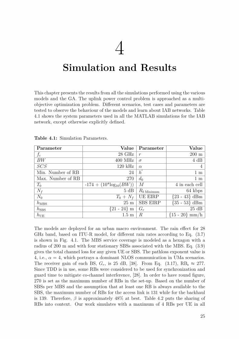
4.12 One cell: Service coverage Probability versus the number of UEs, with1 RB per UE. The maximum number of UEs is 65, with 131 RBs forthe access and 139 RBs for the backhaul. . . . . . . . . . . . . . . . . 34
4.13 One cell: Service coverage Probability versus number of UEs, with 2RBs per UE. The maximum number of UEs is 65, with 131 RBs forthe access and 139 RBs for the backhaul. . . . . . . . . . . . . . . . . 34
4.14 One cell: Service coverage Probability versus the number of UEs,with 3 RBs per UE. The maximum number of UEs is 43, with 131RBs for the access and 139 RBs for the backhaul. . . . . . . . . . . . 35
4.15 One cell: Service coverage Probability versus the number of UEs,with 4 RBs per UE. The maximum number of UEs is 32, with 131RBs for the access and 139 RBs for the backhaul. . . . . . . . . . . . 35
4.16 Two cell: Service coverage probability versus the number of UEs, with1 RB per UE. The maximum number of UEs is 65, with 131 RBs forthe access and 139 RBs for the backhaul. . . . . . . . . . . . . . . . . 37
4.17 Two cell: Service coverage probability versus the number of UEs, with2 RBs per UE. The maximum number of UEs is 65. . . . . . . . . . . 37
4.18 Two cell: Service coverage probability versus the number of UEs, with3 RBs per UE. The maximum number of UEs is 43. . . . . . . . . . . 38
4.19 Two cell: Service coverage probability versus the number of UEs, with4 RBs per UE. The maximum number of UEs is 32. . . . . . . . . . . 38
4.20 One cell: Service coverage probability versus the data rate with 1 RBper UE, Rb = 1 Mbps. The analysis is for the data rate values afterpower control. . . . . . . . . . . . . . . . . . . . . . . . . . . . . . . . 39
4.21 One cell: Service coverage probability versus the data rate with 4RBs per UE, Rb = 5 Mbps. The analysis is for the data rate valuesafter power control. . . . . . . . . . . . . . . . . . . . . . . . . . . . . 40
4.22 One cell special case: Service coverage probability versus the datarate with 1 RB per UE, Rb = 1 Mbps. The analysis is for the datarate values after power control. . . . . . . . . . . . . . . . . . . . . . 41
4.23 One cell special case: Service coverage probability versus the datarate with 4 RBs per UE, Rb = 5 Mbps. The analysis is for the datarate values after power control. . . . . . . . . . . . . . . . . . . . . . 41
4.24 One cell: Service coverage probability versus the number of UEs, with4 RB per UE, E =32, in non-IAB network. . . . . . . . . . . . . . . . 42
4.25 One cell: Service coverage probability versus increasing cell radius,with 4 RBs per UE, from 200 m to 700 m (E = 32). . . . . . . . . . . 43
4.26 CDF for UEs associated with the SBS with fixed cell radius. Theanalysis is for the distribution of the transmit power values afterpower control. . . . . . . . . . . . . . . . . . . . . . . . . . . . . . . . 44
xvi

List of Figures
4.27 CDF for UEs associated with the MBS with fixed cell radius. Theanalysis is for the distribution of the transmit power values afterpower control. . . . . . . . . . . . . . . . . . . . . . . . . . . . . . . . 45
4.28 Plots of the convergence of Genetic Algorithm. Different GA conver-gence plots are captured for different simulations. . . . . . . . . . . . 46
A.1 Service coverage probability versus inter-cell distance. Here, only twoadjacent cells are used for the test, the distance between two cells startfor 0 to 200 m, E = 4, RB = 2 per UE, E = 32. . . . . . . . . . . . I
A.2 Service coverage probability versus intra-cell distance, r = (200 m to700 m), with 1 RB per UE, E = 32, M = 4. . . . . . . . . . . . . . . II
A.3 Service coverage probability versus intra-cell distance, r = (200 m to700 m), with 2 RBs per UE, E = 32, M = 4 . . . . . . . . . . . . . . II
xvii

List of Figures
xviii

List of Tables
2.1 5G NR numerologies [26], [27]. . . . . . . . . . . . . . . . . . . . . . . 11
3.1 Definition of simulation parameters. . . . . . . . . . . . . . . . . . . . 15
4.1 Simulation Parameters. . . . . . . . . . . . . . . . . . . . . . . . . . . 254.2 Empirical sharing of resource blocks. . . . . . . . . . . . . . . . . . . 26
xix

List of Tables
xx

1Introduction
1.1 Background and Motivation
Logically, the telecommunication network is divided into the access network, trans-port network, and the core network, [1]. The access network consists of wireless andwired resources that are used for delivering last-mile services to the users. In wirelessaccess networks, services are mainly delivered via a base station (BS). The BS in a5G network is referred to as the Next Generation NodeB (gNodeB or gNB), [2]. Thetransport network consists of all transmission media and technologies for backhaul-ing and interconnecting all entities within the entire telecom network. Backhaulingis usually achieved with optical fiber and point-to-point microwave links, [3]. Theoptical transport solutions are usually built on wavelength division multiplexing(WDM) and Carrier Ethernet. The core network is the decision layer of the net-work and without it, the network cannot offer any of the intended services. Thecore node of the 5G network is generally referred to as the 5GC. The 5GC handlesinterconnection of the sub-networks or clusters, address and mobility managementof the user equipment (UE), session management, user or data plane management,policy control, authentication, network slicing and other unique functions. 5GC alsohosts the major applications offered by the 5G network, [4], [5].
Historically, there is a growing trend in demand for wireless access solutions. Usersand businesses need more flexibility and cheaper access to their mobile services.Fixed wireless access (FWA) is a viable approach to meet their wireless access de-mands. FWA is more cost effective as compared with fixed broadband last-mile ac-cess like optical fiber, [6]. Using optical fiber links for backhauling and node-to-nodeinterconnection is reliable to a large extent, since it is immune to electromagneticinterference and can support Terabits per second data rates.
Conversely, fiber is expensive to deploy, and it may not be attainable to have iteverywhere. Due to the local geometry and features in some locations, optical fiberinstallations may not be feasible. The cost of maintenance and replacement is alsorelatively high. Then, there are some governing policies in certain locations that donot allow installing new infrastructures for the use of optical fiber. Therefore, theother option in this case is FWA. FWA offers shared point-to-multipoint last-mileservice delivery, unlike fixed broadband connections. It should be noted howeverthat FWA uses the wireless channel which will have to contend with all the factorsaffecting the wireless signal. The varying characteristics of the wireless channel will
1

1. Introduction
lead to varying service quality and data rates for the end users. The varying servicequality also depends on the cell load, [6]. Additionally, the frequency band in usedetermines the coverage of the wireless service, as the transmitters are power lim-ited. Low frequency bands have longer wavelengths and so have a better coveragethan high band frequencies. Typically, wireless backhauling for FWA base stationsrequire a different frequency band which comes at a cost of acquiring separate fre-quency spectrum for both wireless access and backhauling.
Moreover, the 5G wireless network is designed to offer high-rate data streams foreveryone, everywhere, and at any time. 5G comes with a need for a higher channelbandwidth allocation for the radio access network (RAN). In order to support ahigher number of devices per square kilometer, the network needs to be highly den-sified. Basically, point-to-point wireless backhaul links have always been designedbased on line-of-sight (LOS) and non-standardized technologies utilizing high fre-quencies. With 5G in an urban area, the small base stations (SBSs) will be at thestreet level thereby creating a chance for non-line-of-sight (NLOS) in the backhaullinks. Also, the access link, which previously was at low frequencies, is moving tomillimeter wave (mmWave). The mmWave range was previously dedicated to back-haul links. Then, having non-standardized technologies in mmWave backhaul is nomore reasonable, as it will conflict with the access links. These NLOS backhaulingcapabilities and the use of standardized backhauling are the main motivations forIAB networks. Of course, cost, flexibility, and low time-to-market are further moti-vations for both wireless backhaul and IAB networks.
3GPP has offered a multi-hop IAB network solution, with a distributed architecture.Here, each IAB node, or SBS, can be connected to the macro base station (MBS),referred to IAB donor, using the same frequency of the wireless access link. Usingthe same frequency for access and backhaul is called in-band backhauling. On theother hand, out-of-band backhauling is when the backhaul and access links operatein different frequency bands.
In brief, using IAB nodes will further improve the service coverage within a tar-get area. Inherently, using in-band backhauling introduces more interference forthe backhaul links, which may limit the service coverage probability and the actualdata rate that the end-users can achieve. In this scenario, a well-known wirelesscommunication solution is to define a proper network plan about the BS locationsand power levels. However, network planning is an offline approach which does notfactor in real-time channel realizations. If required, dynamic power control and rateadaptation may further improve the service coverage probability, [7], [8].
Power control aims to always have a specific minimum signal-to-interference-plus-noise ratio (SINR) at all times, irrespective of the channel conditions. Although,having the required minimum SINR may not be feasible at all times. On the otherhand, rate adaptation, or rate control, aims to achieve an overall service availabilityas much as possible, by intelligently adjusting the modulation scheme and codingrate of the communication system, according to the prevailing channel conditions.
2

1. Introduction
Power control is usually used in uplink communication, while rate adaptation isusually used in downlink communication, with fixed transmit power from the BSs.
1.2 AimThe aim of the thesis work is to find an appropriate power control scheme for im-plementation in a 5G IAB network. The thesis also put into consideration variousenvironmental factors and constraints that can limit the service coverage and perfor-mance of the 5G IAB network. The objective is to study IAB network performancein uplink communication and achieve the following:
• Identify realistic channel models for mmWave communication in IAB networks.• Identify the appropriate power allocation schemes in IAB networks.• Develop a simulator to evaluate the effect of power allocation in IAB networks.• Carry out comparisons between a single macro-cell network and dual macro-
cell network, with power allocation.
1.3 Thesis ContributionThe thesis tries to answer the following research questions in wireless communicationwith regards to 5G IAB networks.
• Why power control may be useful in IAB networks?• Why is having an efficient power allocation algorithm important in IAB net-
works, like using genetic algorithm (GA)?• What will be the impact of intra-cell and inter-cell interference on service
coverage probability of IAB networks?• What is the benefit of separating access links and backhaul links in IAB net-
works, based on time division duplex (TDD)?
1.4 LimitationsThe thesis investigates power control for the 5G IAB networks in uplink communi-cation. Simulations are carried out with models and parameters suggested by 3GPPfor 5G RAN. The work is not based on real 5G network data. Also, the thesis willnot study the possibility of having simultaneous transmission and reception in IABnetworks. All simulations will be carried out on MATLAB. The simulations will notconsider the 5G network in an end-to-end manner. The thesis is limited to findinga proper power allocation scheme for the uplink channel in the 5G IAB network.
1.5 MethodologyThe thesis is based on a simplified spatial model of a 5G IAB network. The modelfactors in a couple of wireless environmental factors in a well-planned out RAN. Themodel consists of multiple UEs and statically positioned base stations (Macro andSmall BSs), and assumes that only the MBS is connected by non-IAB backhaul,
3

1. Introduction
e.g., fiber, towards the core network. Then, there are a number of SBSs or IABnodes whose traffic are backhauled to the MBS using in-band communication. Themodel tries to maximize the SINR per node using a central GA solution. The GAwill in turn try to maximize the service coverage probability, under the designedIAB conditions. The main measurement metric is the service coverage probability.
1.6 Previous WorkFirst, there are a couple of other related works based on 5G IAB network structureand coverage in downlink communication [9], [10]. In particular, their work providesthe background about IAB network architecture and service coverage in downlinkcommunication. Furthermore, a simulation of the 5G IAB network is made usingthe finite homogeneous Poisson point process (FHPPP) model which uses 28 GHzband, 1 GHz channel bandwidth and sets a minimum data rate of 100 Mbps perUE. Their work specifically compares service coverage with backhaul bandwidth ofthe IAB network.
Then, [11] investigates the actual number of IAB nodes that are needed for anoptimum 5G IAB deployment. Their work simulates a resource scheduling scenariofor 5G IAB using 28 GHz band with 1 GHz bandwidth, characterizing the transmis-sion control protocol-internet protocol (TCP/IP) stack. Their work also identifiespossible challenges in throughput and latency of the related 5G service.
Also, [12] discusses and evaluates the coverage extension improvement in 28 GHzband with IAB deployment in 3GPP Urban micro (UMi) scenarios. Their work com-pares IAB schemes with and without dynamic TDD interference using centralizedscheduling. The simulation-based results show that a fully flexible IAB network canachieve around 60% gain in the uplink and 100% gain in the downlink, as comparedwith non-IAB deployment. Moreover, the scheme without dynamic TDD interfer-ence shows a good gain in downlink communication. The results point to the factthat achieving high spectral efficiency at the backhaul is important for the overallsystem performance.
Additionally, [13] investigates the power allocation problem for a proposed in-bandself-backhaul scheme. The set-up works with multiple antennas with full-duplexcommunication at the BS, which enables the access and backhaul to work simul-taneously within the same frequency band. An iterative algorithm is proposed tosuccessively allocate the powers in the considered scenario so that the users’ sum-rate is maximized, while taking into account the capacity limits of the backhaullink. Then, their work identifies cross-link interference and self-interference, or co-channel interference, as the major challenges that must be mitigated. The resultsshow that the interference between the backhaul and the access networks of in-bandself-backhauled networks is a major limiting factor to the overall system throughput,which can be alleviated using proper power allocation schemes. Moreover, resourcescheduling is considered as a key to having an overall optimal solution.Furthermore, [14] details the IAB network in an end-to-end manner, in line with
4

1. Introduction
3GPP release 16 (Rel-16) proposal. Specifically, their work shows that the IABnetwork still has a half-duplex constraint, even though it can support space divisionmultiplexing (SDM), frequency division duplex (FDD), and TDD.
Interestingly, [15] formulates a multi-hop scheduling problem to propose an effi-cient IAB network deployment. The work further stresses the need for a resourcescheduler and proposes not having more than two hops away from the donor gNB.Reducing the number of hops is to lower the end-to-end network latency, while stillachieving the required data capacity for access and backhauling.
On IAB network topology optimization, [16] looks into using GA formulations forboth IAB node and non-IAB backhaul link distribution. The work makes a case forefficient routing in locations with severe availability constraints and high blockagedensities. Therefore, load balancing the traffic across the network becomes impor-tant in order to improve the service coverage. The work also summarizes the recentRel-16 approved solutions as well as the latest Rel-17 3GPP considerations on traf-fic routing in IAB networks. For a resilient RAN, mesh-based IAB networks areproposed.
Taking a look at future wireless networks, [17] investigates the use of a predic-tor antenna to boost the service performance in moving IAB networks. Mobility ofeither the transmitter or receiver, or both, results in variations in wireless channelconditions. The paper considers having a single antenna mounted on vehicles as amoving IAB node to boost service in both urban and rural areas, with backhaulsupported by either terrestrial or satellite communication. Field trials shows thatmoving IAB nodes offers up to 50% improvement in backhaul throughput as com-pared to open-loop schemes.
Moreover, [18] studies the advantage of scheduling and data rate maximization inIAB networks. The work proposes a minimum throughput maximization algorithmfor IAB networks. The model considers pathloss, directional beamforming, andantenna gain array of the BSs. The simulations are set-up to optimize resourcescheduling of IAB nodes by maximizing the minimum throughput of the accesslinks based on the revised simplex method. The results show that with IAB net-works, there is a possibility to achieve a minimum throughput that out performsMBS only networks.
1.7 Thesis OutlineThe thesis report is arranged to introduce the work and fully detail the work done.Chapter 1 introduces the thesis work. Chapter 2 gives the theoretical backgroundand deployment overview of IAB networks. Chapter 3 explains system models usedand the methodology. Chapter 4 covers the simulations and results. Chapter 5 offersthe conclusions from the thesis work, while Chapter 6 lists the related future workson IAB networks, that could be of interest. Finally, all references and other sourcesof information used are listed.
5

2Theoretical Background
2.1 5G New Radio5G new radio (NR) is the newest radio access air interface of the 5G network. 5G NRoffers a unified and more robust RAN than the previous technologies, such as second-generation (2G), third-generation (3G), and the fourth-generation (4G), [19]. It isspecifically designed to support new generation services and various use cases likevirtual reality (VR) and 4K/8K videos, [20]. Specifically, 5G NR offers a flexiblebandwidth use with similar modulation schemes as 4G. The flexibility of 5G NRsupports different access services in terms of coverage capacity, data rate, and latencyrequirements, [21]. Also, 5G NR comes with improved channel coding, waveformgeneration, massive multiple-input-multiple-output (MIMO), beamforming, networkslicing, improved frame structures, hybrid automatic repeat request (HARQ), andduplexing, [5], [19]. The combination of all these makes it far superior to the previoustechnologies. Fig. 2.1 illustrates the 5G NR use cases.
Figure 2.1: Illustration of 5G NR use cases. 5G NR services are classified aseMMB, URLLC and mMTC.
6
2. Theoretical Background
As a standard, 5G services are classified into three categories. These are enhancedmobile broadband (eMBB), massive machine-type communication (mMTC), andultra-reliable and low-latency communication (uRLLC), [22].
5G promises improved user experience with a latency down to 1 ms, over the wire-less channel, data rates of between 100 Mbps and 1 Gbps per UE, and Terabits persecond data rate per square kilometer. There are on-going studies for 5G to supportmobility of up to 300 km/h, [23]. Also, 5G NR uses orthogonal frequency divisionmultiplexing (OFDM) technology, which is a widely used spectrally efficient wirelessaccess technology. OFDM is already in use in IEEE 802.11 wireless fidelity (Wi-Fi), Worldwide Interoperability for Microwave Access (WiMAX), and 4G long-termevolution (LTE).
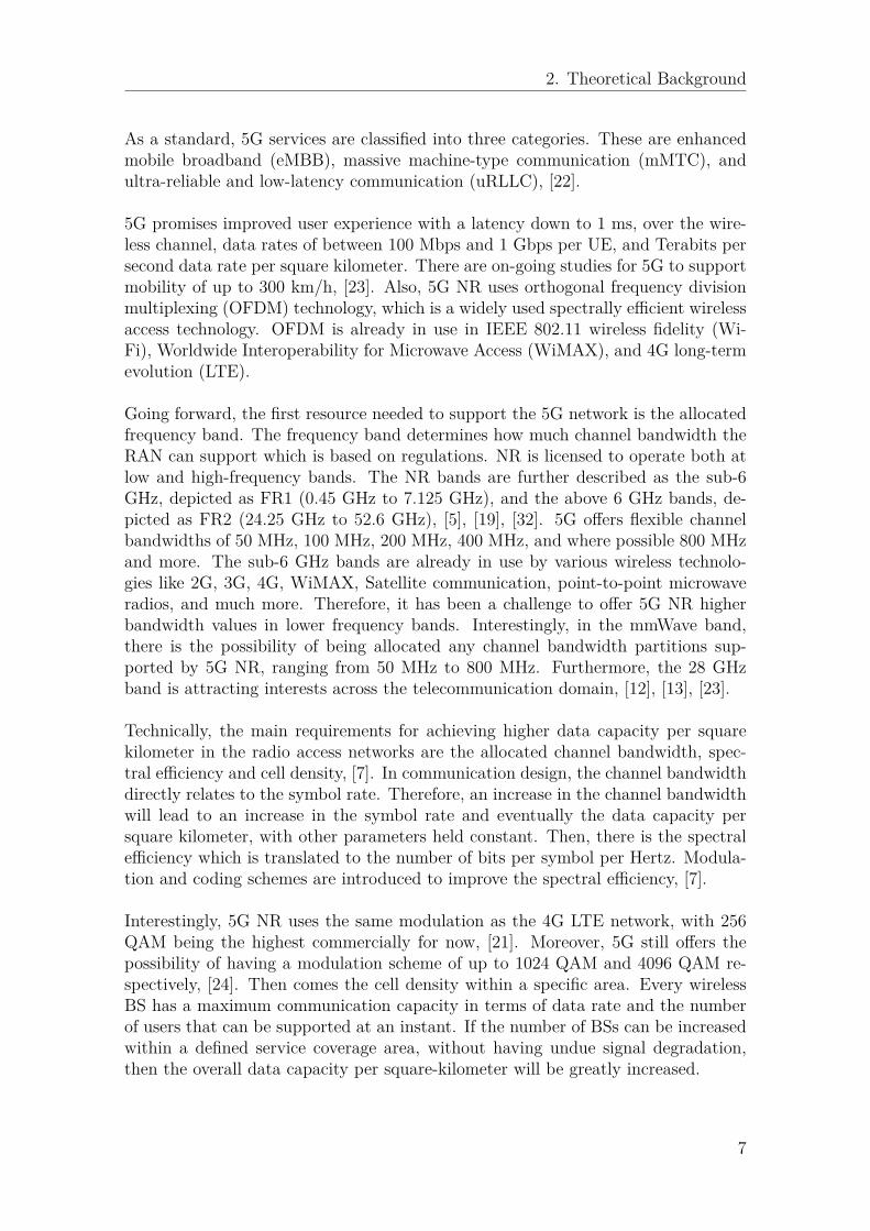
Going forward, the first resource needed to support the 5G network is the allocatedfrequency band. The frequency band determines how much channel bandwidth theRAN can support which is based on regulations. NR is licensed to operate both atlow and high-frequency bands. The NR bands are further described as the sub-6GHz, depicted as FR1 (0.45 GHz to 7.125 GHz), and the above 6 GHz bands, de-picted as FR2 (24.25 GHz to 52.6 GHz), [5], [19], [32]. 5G offers flexible channelbandwidths of 50 MHz, 100 MHz, 200 MHz, 400 MHz, and where possible 800 MHzand more. The sub-6 GHz bands are already in use by various wireless technolo-gies like 2G, 3G, 4G, WiMAX, Satellite communication, point-to-point microwaveradios, and much more. Therefore, it has been a challenge to offer 5G NR higherbandwidth values in lower frequency bands. Interestingly, in the mmWave band,there is the possibility of being allocated any channel bandwidth partitions sup-ported by 5G NR, ranging from 50 MHz to 800 MHz. Furthermore, the 28 GHzband is attracting interests across the telecommunication domain, [12], [13], [23].
Technically, the main requirements for achieving higher data capacity per squarekilometer in the radio access networks are the allocated channel bandwidth, spec-tral efficiency and cell density, [7]. In communication design, the channel bandwidthdirectly relates to the symbol rate. Therefore, an increase in the channel bandwidthwill lead to an increase in the symbol rate and eventually the data capacity persquare kilometer, with other parameters held constant. Then, there is the spectralefficiency which is translated to the number of bits per symbol per Hertz. Modula-tion and coding schemes are introduced to improve the spectral efficiency, [7].
Interestingly, 5G NR uses the same modulation as the 4G LTE network, with 256QAM being the highest commercially for now, [21]. Moreover, 5G still offers thepossibility of having a modulation scheme of up to 1024 QAM and 4096 QAM re-spectively, [24]. Then comes the cell density within a specific area. Every wirelessBS has a maximum communication capacity in terms of data rate and the numberof users that can be supported at an instant. If the number of BSs can be increasedwithin a defined service coverage area, without having undue signal degradation,then the overall data capacity per square-kilometer will be greatly increased.
7
2. Theoretical Background
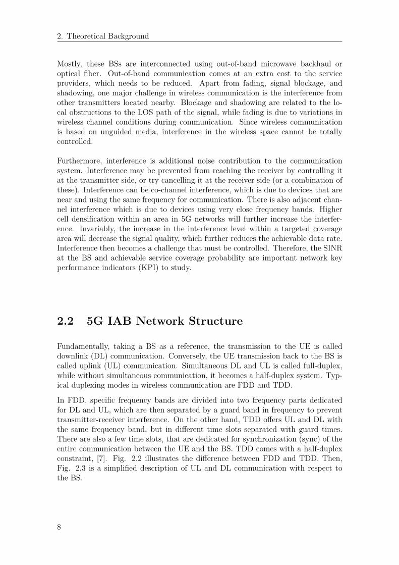
Mostly, these BSs are interconnected using out-of-band microwave backhaul oroptical fiber. Out-of-band communication comes at an extra cost to the serviceproviders, which needs to be reduced. Apart from fading, signal blockage, andshadowing, one major challenge in wireless communication is the interference fromother transmitters located nearby. Blockage and shadowing are related to the lo-cal obstructions to the LOS path of the signal, while fading is due to variations inwireless channel conditions during communication. Since wireless communicationis based on unguided media, interference in the wireless space cannot be totallycontrolled.
Furthermore, interference is additional noise contribution to the communicationsystem. Interference may be prevented from reaching the receiver by controlling itat the transmitter side, or try cancelling it at the receiver side (or a combination ofthese). Interference can be co-channel interference, which is due to devices that arenear and using the same frequency for communication. There is also adjacent chan-nel interference which is due to devices using very close frequency bands. Highercell densification within an area in 5G networks will further increase the interfer-ence. Invariably, the increase in the interference level within a targeted coveragearea will decrease the signal quality, which further reduces the achievable data rate.Interference then becomes a challenge that must be controlled. Therefore, the SINRat the BS and achievable service coverage probability are important network keyperformance indicators (KPI) to study.
2.2 5G IAB Network Structure
Fundamentally, taking a BS as a reference, the transmission to the UE is calleddownlink (DL) communication. Conversely, the UE transmission back to the BS iscalled uplink (UL) communication. Simultaneous DL and UL is called full-duplex,while without simultaneous communication, it becomes a half-duplex system. Typ-ical duplexing modes in wireless communication are FDD and TDD.
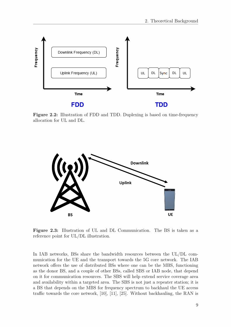
In FDD, specific frequency bands are divided into two frequency parts dedicatedfor DL and UL, which are then separated by a guard band in frequency to preventtransmitter-receiver interference. On the other hand, TDD offers UL and DL withthe same frequency band, but in different time slots separated with guard times.There are also a few time slots, that are dedicated for synchronization (sync) of theentire communication between the UE and the BS. TDD comes with a half-duplexconstraint, [7]. Fig. 2.2 illustrates the difference between FDD and TDD. Then,Fig. 2.3 is a simplified description of UL and DL communication with respect tothe BS.
8
2. Theoretical Background
Figure 2.2: Illustration of FDD and TDD. Duplexing is based on time-frequencyallocation for UL and DL.
Figure 2.3: Illustration of UL and DL Communication. The BS is taken as areference point for UL/DL illustration.
In IAB networks, BSs share the bandwidth resources between the UL/DL com-munication for the UE and the transport towards the 5G core network. The IABnetwork offers the use of distributed BSs where one can be the MBS, functioningas the donor BS, and a couple of other BSs, called SBS or IAB node, that dependon it for communication resources. The SBS will help extend service coverage areaand availability within a targeted area. The SBS is not just a repeater station; it isa BS that depends on the MBS for frequency spectrum to backhaul the UE accesstraffic towards the core network, [10], [11], [25]. Without backhauling, the RAN is
9

2. Theoretical Background
incomplete. Backhauling is therefore critical in building a functional RAN. In thisreport, SBS and IAB nodes are used interchangeably.
Figure 2.4 is an illustration of the 5G IAB network. There is one MBS, i.e., IABdonor, with four SBSs, i.e., IAB nodes, connected to it via wireless backhaul links.The MBS is directly connected to the 5GC via non-IAB backhaul, e.g., optical fiber,and both the MBS and the SBSs are offering wireless access connections to the UEs.Eventually, all the data capacity within the service coverage area of the MBS is de-pendent on non-IAB backhaul, e.g., optical fiber, to connect to the 5GC. Moreover,all the SBSs and UEs within this service coverage area will be sharing the channelbandwidth that is allocated to the MBS. The MBS may connect to multiple SBSsand the SBSs may support multiple UEs. In general, IAB networks support anarbitrary number of hops from the MBS to the last-mile UE. The MBS, by virtueof the antenna design, supports massive MIMO. The narrowness of the beams fromthe MBS and SBSs in the downlink direction depicts beamforming towards specificSBSs and UEs. Based on the considered resource allocation strategy, a fraction ofthe channel bandwidth will be used for the access link, and the other bandwidthpart will be used by the backhaul links.
Figure 2.4: Illustration of 5G IAB network. There is one central MBS and fourother SBSs depend on it for backhauling.
10

2. Theoretical Background
Table 2.1: 5G NR numerologies [26], [27].
Numerology (µ) Sub-carrier spacing (kHz) Slot Duration (ms) Bandwidth (MHz)0 15 1 501 30 0.5 1002 60 0.25 2003 120 0.125 4004 240 0.0625 400, 800
Furthermore, an IAB network with a long chain of dependent SBSs may increasethe end-to-end latency and cause backhaul congestion. High latency is an unwantedeffect in IAB networks. Although, it is theoretically possible to have multiple hops,it is suggested to limit the number of hops in the IAB network to 2, [16]. Also,since the access and backhaul will be sharing the same frequency spectrum, thencross-link interference will be present. Cross-link interference is when BSs interferewith one another because they transmit and receive in the same spectrum and atthe same time. Therefore, TDD is a viable option but it comes with a half-duplexconstraint, in order to reduce interference. With TDD, the UEs are constrained toonly periodic transmission and reception, which results in a lower capacity whencompared with FDD. There are ongoing studies on how to achieve simultaneoustransmission within IAB networks, [25].
Practically, 5G NR is based on OFDM using closely packed modulated sub-carriersignals, [26]. Each sub-carrier has its own bandwidth, or sub-carrier spacing (SCS).SCS is also referred to as NR numerology. NR offers various SCS values ranging from15 kHz, 30 kHz, 60 kHz, 120 kHz, up to 240 kHz, [26], [27]. SCS of 120 kHz and240 kHz are suggested for FR2 mmWave bands, because they can easily support400 MHz and 800 MHz channel bandwidth respectively, [26]. A finite number ofcontiguous sub-carriers are then made into resource blocks (RB). One RB is definedas 12 consecutive sub-carriers in the frequency domain. Also, RB is the smallesttime-frequency resource that can be allocated to a UE in OFDM systems. Therefore,the wireless BS will support a finite number of RBs based on the allocated channelbandwidth, [26]. Table 2.1 shows the 5G NR numerologies in this context. Then,Fig. 2.5 shows how RBs are shared between access and backhaul links.
Both the MBS and SBSs are capable of independently administering the channelbandwidth. Since only the MBS has a non-IAB backhaul, e.g., an optical fiberconnection, towards the core network, then the SBSs must depend on the MBS fortheir backhaul bandwidth. Certain RBs are used for the interconnection betweenthe MBS and the SBSs, which becomes the backhaul link for the SBSs. Then, otherRBs can be used by the UEs to access the network. By the RBs sharing approach,the MBS can serve both UEs and SBSs at the same time. The access traffic fromthe UEs connected to an SBS will have to be switched from the RBs used in theaccess link to the RBs used in the backhaul link. Fig. 2.5 depicts all of these incontext.
11

2. Theoretical Background
Figure 2.5: Resource sharing between MBS, SBS and UE. From [29]. Reproducedwith permission.
2.3 Structure of IAB NodesThe 5G NR structure, as standardized by 3GPP, supports a distributed architecture,[30]. The traditional deployment from 2G, 3G and even 4G LTE basically offers oneMBS per location. However, the architecture of the BS in 5G has been separatedinto a central unit (CU) and a distributed unit (DU). IAB donor, i.e., MBS, is CUand DU combined, while the IAB nodes, i.e., SBSs, are mobile terminal (MT) andDU combined. The MT has similar functionalities as a UE. The MBS can supporta finite number of SBSs within a specified location. Also, each of the IAB nodehas a finite number of UEs that can be supported at an instant. The CU/DU andDU/MT model is illustrated in Fig. 2.6.
2.4 The Role of Power Control in IAB NetworksPower control in wireless communication is a solution deployed to control the trans-mit power of the UEs in order to achieve an overall efficient communication system.Also, power control is an intelligent approach to reduce the power consumption of
12

2. Theoretical Background
Figure 2.6: The Architecture of SBS/IAB nodes.
a transceiver device, which can either be a UE or a BS. In uplink communication,power control reduces the UE power consumption and the interference (inter, in-tra and co-channel interference), thereby increasing the service coverage probability,while reducing the outage probability. Typically, the more the interference power,the lower the SINR at the receiver, and the lower the achievable data rates, [13], [14].Interestingly, to achieve high data rates in wireless communication comes at the costof transmit power and SINR, irrespective of the channel noise and interference. Apower allocation scheme tries to achieve the baseline SINR requirement, by dynamictransmit power assignment to the UEs irrespective of the prevailing channel condi-tions. Furthermore, power control is an important approach in maximizing cellularnetwork capacity, by increasing the number of UEs that can be serviced within anarea. Power control also helps to protect the BS receiver’s circuit from power over-load, which can damage the entire transceiver system.
In mobile communication, UEs are randomly distributed due to their mobility. Dueto their mobility, the UE transmit power requirement varies per location and time.Power control is necessary to keep the power levels down based on global telecom-munication regulations. Practically, all transmitters are power limited. Generally,UEs are classified into transmit power classes, [28].
Typically, users that are closer to the BSs transmit lower power than users thatare far off. The UEs transmit at lower power because the magnitude of the pathlossis distance dependent, i.e., pathloss grows with distance away from the target BS.Controlling the power level of the UEs will help create a balanced received powerlevel at the BS. Fading effect in the channel is also mitigated with power control.IAB networks bring the BSs closer to the users, thereby reducing their transmitpower requirement and improving the users’ experience.
13
3System Model
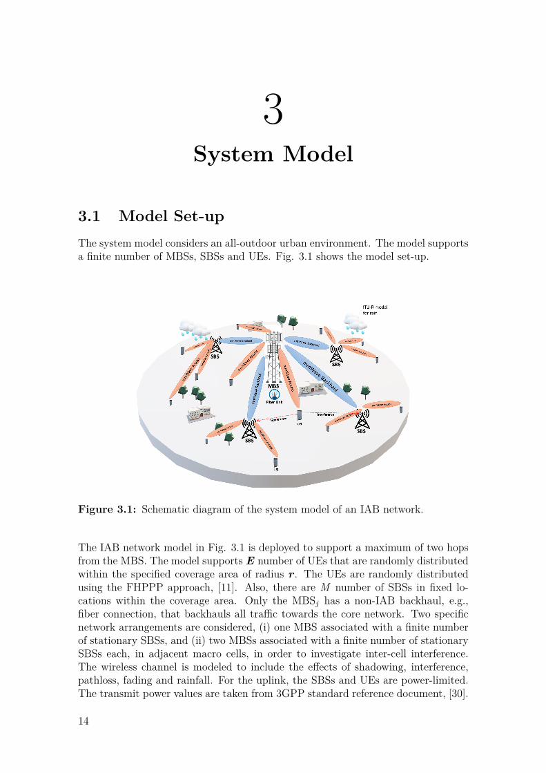
3.1 Model Set-upThe system model considers an all-outdoor urban environment. The model supportsa finite number of MBSs, SBSs and UEs. Fig. 3.1 shows the model set-up.
Figure 3.1: Schematic diagram of the system model of an IAB network.
The IAB network model in Fig. 3.1 is deployed to support a maximum of two hopsfrom the MBS. The model supports E number of UEs that are randomly distributedwithin the specified coverage area of radius r . The UEs are randomly distributedusing the FHPPP approach, [11]. Also, there are M number of SBSs in fixed lo-cations within the coverage area. Only the MBSj has a non-IAB backhaul, e.g.,fiber connection, that backhauls all traffic towards the core network. Two specificnetwork arrangements are considered, (i) one MBS associated with a finite numberof stationary SBSs, and (ii) two MBSs associated with a finite number of stationarySBSs each, in adjacent macro cells, in order to investigate inter-cell interference.The wireless channel is modeled to include the effects of shadowing, interference,pathloss, fading and rainfall. For the uplink, the SBSs and UEs are power-limited.The transmit power values are taken from 3GPP standard reference document, [30].
14

3. System Model
There is an arbitrary RB scheduler that governs the communication among theMBSs, SBSs and UEs.
Table 3.1: Definition of simulation parameters.Parameter Definition Parameter Definitionr Cell radius BW BandwidthE Total number of UE Em Number of UEs that met minimum requirement of the serviceM Number of SBS BWRB Bandwidth for one resource blockd2D 2D distance T0 Thermal noised3D 3D distance U Set of UE in coverage areaPEIRP Effective Isotropic Radiated Power Gr Receiver gainα Path-loss exponent c Speed of lightσ Shadowing loss CH Channel capacityPt Transmission power RBs Number of resource blockPr Received power EAccessUE Number of user related to access linkRCV Receiver sensitivity Γ Polarization coefficientL Path-loss k Polarization coefficientRB Resource block φ Fading effectRb Data rate E Number of UEγR Rain losses Z Set of SBS in coverage areadBP Break point distance N0 Total noisefc Carrier frequency Nf Noise figurehBS Base station Height SCS Sub-carrier spacinghUE UE height h
′UE Effective height for UE
h′BS Effective height of the base station β The percentage of the bandwidth resourcesN total number of iteration K Number of first iteration group in GAS Number of second iteration group in GA V Third number of iteration in GAXI In-phase channel realization XQ Quadrature channel realizationA Set of associated UEs W Set of associated SBSsd0 Reference distance ρ Service coverage probabilityR Rain rate t TimeI Interference SINR Signal to interference plus noise
The following are the general assumptions made for our work.
• An OFDM multi-access solution with a TDD duplexing option.• A central TDD scheduler governs the communication of the base stations and
UEs.• MBS has 3 sectorial antennas, at 120 degrees each for a complete 360 degree
coverage per base station, [31].• The frequency band is 28 GHz, and the allocated channel bandwidth is 400
MHz (27.8 GHz to 28.2 GHz), [5].• UEs can use different RBs per time slot, since they are assumed to be mobile
and the wireless channel characteristics vary from time to time.• The transmit power of the UE and SBS is taken as the effective isotropic
radiated power (EIRP). EIRP is the transmit power plus the antenna gain, indecibel scale.
• Periodic access to channel state information (CSI) is available at the UE, SBSand MBS.
• The power control problem is treated as a multi-objective optimization prob-lem.
15
3. System Model
3.2 Channel Modelling
3.2.1 Received PowerThe received power at either the MBS or SBS is modelled as:
Pr = Pt +Gt +Gr − L− σ − γR − φ. (3.1)
Here, Pt is the transmit power, Gt is the gain of the transmitter, Gr is the gainof the receiver, L is pathloss, σ is shadowing loss, γR is rain loss, φ is the channelfading effect. All values are in dB. In our work, the transmit power values used areEIRP 3GPP defined values, where PEIRP is expressed as
PEIRP = Pt +Gt. (3.2)
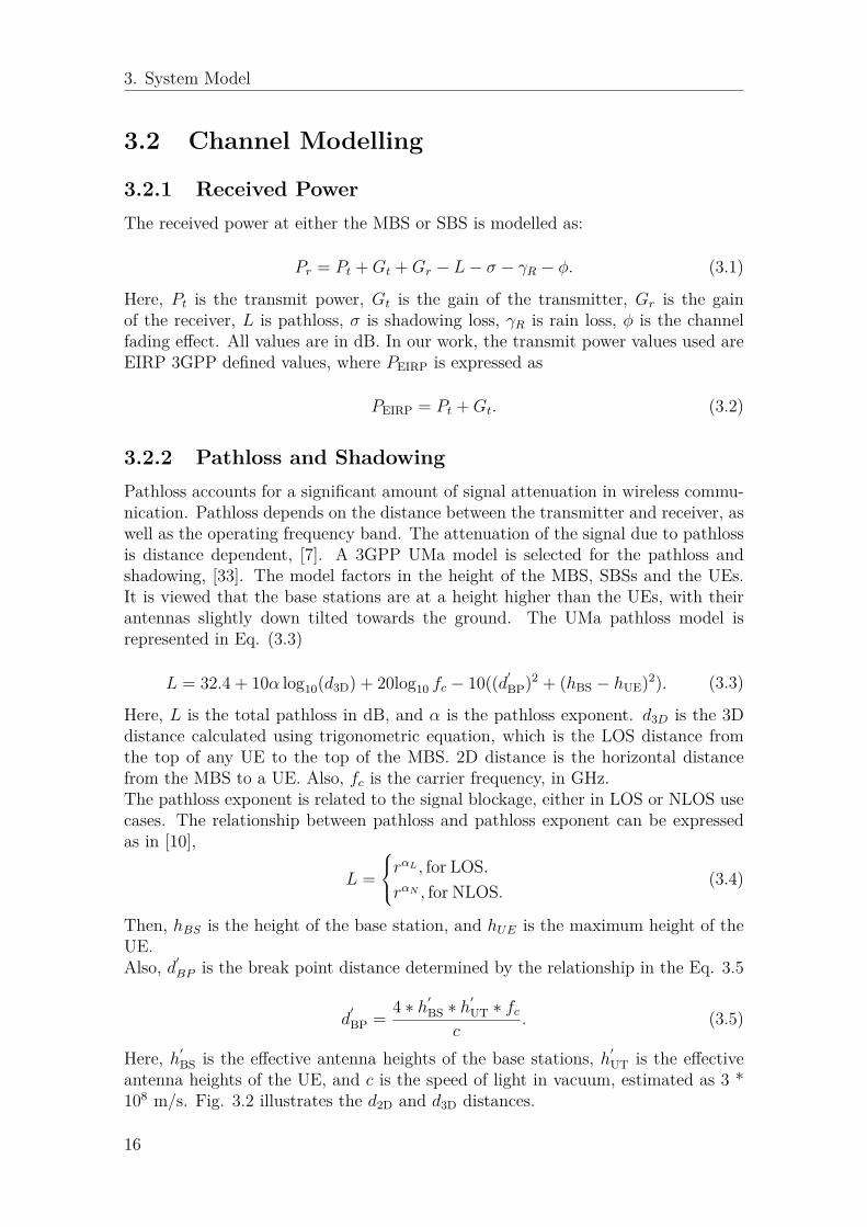
3.2.2 Pathloss and ShadowingPathloss accounts for a significant amount of signal attenuation in wireless commu-nication. Pathloss depends on the distance between the transmitter and receiver, aswell as the operating frequency band. The attenuation of the signal due to pathlossis distance dependent, [7]. A 3GPP UMa model is selected for the pathloss andshadowing, [33]. The model factors in the height of the MBS, SBSs and the UEs.It is viewed that the base stations are at a height higher than the UEs, with theirantennas slightly down tilted towards the ground. The UMa pathloss model isrepresented in Eq. (3.3)
L = 32.4 + 10α log10(d3D) + 20log10 fc − 10((d′
BP)2 + (hBS − hUE)2). (3.3)
Here, L is the total pathloss in dB, and α is the pathloss exponent. d3D is the 3Ddistance calculated using trigonometric equation, which is the LOS distance fromthe top of any UE to the top of the MBS. 2D distance is the horizontal distancefrom the MBS to a UE. Also, fc is the carrier frequency, in GHz.The pathloss exponent is related to the signal blockage, either in LOS or NLOS usecases. The relationship between pathloss and pathloss exponent can be expressedas in [10],
L =
rαL , for LOS.rαN , for NLOS.
(3.4)
Then, hBS is the height of the base station, and hUE is the maximum height of theUE.Also, d′
BP is the break point distance determined by the relationship in the Eq. 3.5
d′
BP = 4 ∗ h′BS ∗ h
′UT ∗ fc
c. (3.5)
Here, h′BS is the effective antenna heights of the base stations, h′
UT is the effectiveantenna heights of the UE, and c is the speed of light in vacuum, estimated as 3 *108 m/s. Fig. 3.2 illustrates the d2D and d3D distances.
16

3. System Model
Figure 3.2: Illustration of d2D and d3D distances. From [33]. Reproduced withpermission.
Shadowing is signal attenuation due to obstructions in the LOS path between thetransmitter and the receiver. The magnitude of shadowing is proportional to thelength of the obstacle. The common shadowing model is log-normal, i.e., ratio oftransmit power to received power in linear scale, [7],
σ = PtPr. (3.6)
3.2.3 Rain EffectIn mmMwave communication, the rain loss is not negligible, [34]. The InternationalTelecommunications Union Radio communication (ITU-R) section already has amodel for corresponding signal attenuation for a given rain rate and operating fre-quency band, [35]. The model is built on a relatively low rain rate of between 15mm/h and 20 mm/h, [34]. The signal attenuation due to rainfall is denoted as γR.The ITU-R power-law relationship model is expressed in Eq. (3.7)
γR = k ∗RΓ. (3.7)
Here, γR is the signal specific attenuation expressed in dB/km, while R is the givenrain rate in mm/h. Then, k and Γ are polarization coefficients that are determinedbased on the operating frequency band. In ITU-R model, the supported frequencyranges from 1 GHz to 1000 GHz, [35]. Finally, in our work, the effect of foliage isassumed to be negligible in urban macro environments.
17

3. System Model
3.2.4 Fading EffectFading is due to variations in the wireless channel conditions. In our work, fadingis modeled as a Rayleigh flat fading channel. Rayleigh distribution is zero-mean,with a unit-variance complex Gaussian distribution, X ∼ N (µ, σ2) , [7]. Rayleighfading is modeled as
φ(t) = XI(t) + jXQ(t). (3.8)Here, φ(t) is the channel realization at time (t) based on Gaussian distribution,XI is the in-phase component of the channel realization, and XQ is the quadraturecomponent of the channel realization.
3.2.5 Total Channel LossThe entire channel effect is taken as a summation of all the above listed signal losscomponents, in decibel. The total channel loss is expressed as
Ploss = L+ σ + γR + φ. (3.9)
Here, L, σ, γR and φ values are all in dB. The inverse of the channel loss value inthe linear scale will give the channel gain.
3.3 InterferenceIn our work, signal interference is taken as the summation of every other receivedpower at a reference point, MBS or SBS, apart from the dominant signal we areinterested in. Interference is expressed as
IUEi =∑
PEIRPj +Grj− Lj − σj − γRj
− φj. (3.10)
3.4 SINR and Baseline SINR ValueSINR refers to the capability of the channel to transmit information. SINR is usuallyused to estimate the quality of the received signal. SINR is the dominant receivedsignal power divided by the sum of all other received signal power plus the noise inthe channel. The SINR, Pr and interference, I are related as
SINR = PrI +N0
. (3.11)
Here, N0 is the modeled channel noise, which is a summation of the noise figureof the receiver, Nf , and the thermal noise, T0. Then, I is the summation of allinterference powers.Given a baseline SINR value and the UE operating bandwidth, the achievable datarate of the channel is thus calculated as
Rb = BW ∗ log2(1 + SINR). (3.12)
18

3. System Model
Here, Rb is the achievable data rate in bits per second, and BW is the channel Band-width, in Hz. In other words, if given a target data rate and operating bandwidth,the minimum SINR, SINRmin, required per UE is determined by
SINRmin = 2Rb
BW − 1. (3.13)
Then the value is converted to decibel (dB) by the expression below:
SINRdB = 10 ∗ log10(SINRmin) (3.14)
3.5 Receiver SensitivityReceiver sensitivity is the minimum received power that can be detected at thereceiver for useful communication. In our work, the receiver is the BS and thereceiver sensitivity must satisfy the minimum SINR value required per UE. Receiversensitivity is therefore expressed as
RCV = SINRmin +N0. (3.15)
Here, SINRmin is the minimum SINR to guarantee the modeled minimum data rateper UE. All values are in dB.
3.6 Resource Block5G NR offers a flexible channel bandwidth based on the SCS value selected. Thebandwidth occupied by an RB depends on the SCS value in use. Our model assumesthat one UE uses a minimum of one RB at a given time. The bandwidth capacityfor one RB is determined by
BWRB = 12 ∗ SCS. (3.16)
Here, BWRB is the bandwidth occupied by one RB, and 12 represents the 12 con-secutive sub-carriers in one RB. It also taken that there is always at least one RBavailable for each SBS at all times. The total number of RBs is determined by
RBs = BW
BWRB
. (3.17)
3.7 UE and SBS AssociationThe UE association is based on the CSI the UE receives from the MBS and SBSperiodically. The SBS association is based on the CSI the SBS receives from theMBS periodically. The UE after receiving the CSI from all the BSs, will determineits channel quality to all the BSs, from its present location. After comparison,the UE will be associated with the BS, MBS or SBS, that offers the best channelquality at that time. Here, the best channel quality means the channel that offersthe highest received signal power at the BS. Likewise, the SBS will associate with
19

3. System Model
the MBS that offers the best channel quality at a given time. The SBSs are allstationary. The association strategy for the UE is expressed as
A =
1, if Pri ≥ PrA,∀ A ∈ U,0, otherwise,
(3.18)
where A is a number of UEs associated with a BS and U is a set of all the UEswithin the service coverage area. Association can be to MBS or to SBSj. On theother hand, the association strategy for the SBS is expressed as
W =
1, ifPri ≥ PrW,∀W ∈ Z,0, otherwise,
(3.19)
where W is the number of SBSs associated with the MBS and Z is a set of all theSBSs within the service coverage area.
3.8 Service Coverage ProbabilityFor our work, service coverage probability (ρ) is defined as the ratio of the UEs withinthe target coverage area that can meet the minimum requirements of SINR valueand data rate at a given instant, to the total number of UEs transmitting within thecoverage area of the MBS. Also, ρ is expressed as a percentage. The major controlmetric for our simulations is ρ. Service coverage probability is expressed as
ρ = EmE× 100. (3.20)
Here, Em is the number of UEs that meet the minimum requirements for the serviceand E is the total number of UEs randomly placed within the targeted servicecoverage area, using FHPPP.
3.9 Achievable Data Rate of the UEThe achievable data rate of a UE within the service coverage is the amount of datathat UE can transmit to its associated BS. The same concept holds for any SBSassociated with a MBS. It is modeled as
Rb = BW ∗ log2(1 + SINRi). (3.21)
Here, SINRi is the SINR value at the receiver side of the BS for a given UEi.
3.10 Access and Backhaul Bandwidth UtilizationBased on the allocated bandwidth, the maximum number of RBs that the wirelesschannel supports is 270. These RBs are shared between the access links and backhaullinks depending on the instantaneous demand from the UEs and SBS. Then, the
20

3. System Model
access bandwidth is directly related to the number of UEs that are associated withthe MBS or SBS at a given time, and the number of RBs per UE. Whereas, thebackhaul bandwidth is directly related to the total number of RBs used in accesslink by the UEs plus the total number of RBs pre-allocated to the SBS. Since 1 RBtranslates to a finite bandwidth value, then the access bandwidth is expressed as
BWAccess = BWRB ∗RBs ∗ EAccessUE. (3.22)With the channel bandwidth being shared between the access and backhaul links,the expression below holdsBWAccess, = β BW.
BWBackhaul, = (1− β)BW.(3.23)
Here, EAccessUE is the total number of UEs associated with the MBS and SBSs,BWAccess is the instant access bandwidth in use, and BWBackhaul is the instantbackhaul bandwidth in use. BWAccess and BWBackhaul can then be weighed againstthe allocated channel bandwidth, BW. The percentage of the bandwidth resourcesused in the access links is represented as β, where β ∈ [0,1].
3.11 TDD Scheduler for MBS/SBS/UEBased on the assumption that all nodes are centrally synchronized and transmissionfrom all nodes are scheduled, the following TDD scheduling epochs are consideredas the transmission time for the MBS, SBS and UE within the network in uplinkcommunication.
(i) When the SBS is transmitting, Fig. 3.3, the MBS and UE are receiving. Inter-ference is only among the SBSs.
Figure 3.3: First TDD Epoch. Here, only SBSs are transmitting within the cell.
21

3. System Model
(ii) When the UE is transmitting, Fig. 3.4, the MBS and SBSs are receiving. Inter-ference is only among the UEs inside the coverage area of the MBS.
Figure 3.4: Second TDD Epoch. Here, only the UEs are transmitting within thecell.
(iii) Special case: when the SBS and UEs associated with the MBS only are trans-mitting, Fig. 3.5. Here, all other UEs and the MBS are receiving. The specialcase creates an opportunity to observe the effect of having the access and backhaulcommunication happening at the same time.
Figure 3.5: Special TDD case. Here, only the SBSs and the UEs associated withthe MBS are transmitting.
22

3. System Model
3.12 Genetic Algorithm for Power ControlA baseline algorithm is needed for proper evaluation of the solutions to the formu-lated power control problem. Also, with a baseline algorithm the entire process isbroken into clear steps, detailing possible aspects that may be refined and allowinglogical inferences to be drawn from the results. For this reason, GA is selected as abaseline algorithm for a proper solution to the problem formulation, [39]- [42]. GA isindependent of the channel realizations which means that the final solutions offeredby the algorithm are comparatively fair. The GA transmit power control algorithmis formally expressed as
Algorithm 1 GA-Transmit Power Control AlgorithmFor each instance in N , with a set of MT that require power control, do the following:
1: Create K, e.g., K = 10, sets of transmit powers, randomly selected from therange between the minimum and maximum transmit power allowed for the MT.Each element in the set corresponds to a MT.
2: For each set, calculate the received power, SINR and outage probability.3: Find the set with the lowest outage probability and set it as the queen.4: Create S�K, e.g., S = 5, sets of randomly selected transmit powers around
the queen. Then, calculate the received power, SINR and outage probability foreach set.
5: Find the set that has the lowest outage probability and update the queen.6: Create a V = K − S − 1 sets of transmit powers, with each element in the set
related to the allowed transmit power for the MT.7: Calculate the received power, SINR and the outage probability of the V set.8: Compare the set which has the lowest outage probability with the queen. Then
choose the one with the lowest outage probability as the queen.9: Then go to back to Step 2 and continue for N iterations.
10: Finally, return the queen as the optimal power solution which has lowest outageprobability after N iterations.
The proposed GA algorithm is thus explained:
A value, N , is set as the number of iterations for the algorithm. The value isdecided by the designer as the maximum number of iterations supported by the al-gorithm. As an example, N = 20. The first step starts by the selection of K numberof iterations randomly, as a part of N iterations. As an example, K = 10. Then, aset is created containing randomly selected transmit powers, with each value comingfrom the pre-defined range of transmit power values supported by the MT. There isa minimum and maximum transmitted power allowed by 3GPP, based on the powerclass of the UEs. Next, the received power of that MT at the BS is calculated, aswell as its corresponding SINR, and outage probability. Outage probability is theprobability of the event that the UEs cannot meet the baseline service requirements.The process is then repeated for K number of iterations. At the end of K iterations,a set of transmit powers that offers the minimum outage probability is selected forK. The newly selected set is set as queen, and is kept for the next step. The second
23

3. System Model
step begins with generating S << K sets of transmit power values around the queen,by making few mutations on it, i.e., changing one or two elements inside the queen.Next, the received power, SINR, and outage probability for each set is calculated.After that, the set with the minimum outage probability is selected and the queenis updated with new values. Therefore, a new queen is created. Going forward, thethird step repeats the first step, which now offers a new queen value. Then, there isa comparison between the new queen from third step and the queen from the secondstep, to see which of them has the lowest outage probability. Finally, the set withthe lowest outage probability now becomes the queen. The algorithm repeats allthe three steps along N and takes the set that offers the lowest outage probabilityas the output.
24
4Simulation and Results
This chapter presents the results from all the simulations performed using the variousmodels and the GA. The uplink power control problem is approached as a multi-objective optimization problem. Different scenarios, test cases and parameters aretested to observe the behaviour of the models and learn about IAB networks. Table4.1 shows the system parameters used in all the MATLAB simulations for the IABnetwork, except otherwise explicitly defined.
Table 4.1: Simulation Parameters.
Parameter Value Parameter Valuefc 28 GHz r 200 mBW 400 MHz σ 4 dBSCS 120 kHz α 4Min. Number of RB 24 h
′ 1 mMax. Number of RB 270 d0 1 mT0 -174 + (10*log10(BW )) M 4 in each cellNf 5 dB Rb Minimum 64 kbpsN0 T0 + Nf UE EIRP {23 - 43} dBmhMBS 25 m SBS EIRP {35 - 53} dBmhSBS {21 - 24} m Gr 25 dBhUE 1.5 m R {15 - 20} mm/h
The models are deployed for an urban macro environment. The rain effect for 28GHz band, based on ITU-R model, for different rain rates according to Eq. (3.7)is shown in Fig. 4.1. The MBS service coverage is modeled as a hexagon with aradius of 200 m and with four stationary SBSs associated with the MBS. Eq. (3.9)gives the total channel loss for any given UE or SBS. The pathloss exponent value is4, i.e., α = 4, which portrays a dominant NLOS communication in UMa scenarios.The receiver gain of each BS, Gr, is 25 dB, [38]. From Eq. (3.17), RBs ≈ 277.Since TDD is in use, some RBs were considered to be used for synchronization andguard time to mitigate co-channel interference, [28]. In order to have round figure,270 is set as the maximum number of RBs in the set-up. Based on the number ofSBSs per MBS and the assumption that at least one RB is always available to theSBS, the maximum number of RBs for the access link is 131 while for the backhaulis 139. Therefore, β is approximately 48% at best. Table 4.2 puts the sharing ofRBs into context. Our work simulates with a maximum of 4 RBs per UE in all
25

4. Simulation and Results
cases. The baseline parameters are based on data rate, SINR, cell radius, RBs perUE, and the concurrent number of UEs within the cell. The KPI of interest is theservice coverage probability, ρ. The minimum data rate of 64 kbps is selected basedon the 3GPP as the minimum data rate for any UE to pass the integrity test in5G NR, [36]. Table 4.2 shows a relationship between the allocated RBs per UE,access-backhaul RB utilization and the number of guaranteed UEs at a time withinthe cell. Analysis from Table 4.2 forms a basis for the upper limit of the number ofUEs simulated in this work.Table 4.2: Empirical sharing of resource blocks.
RB per UE Number of Access RBs Number of Backhaul RBs Total RBs Supported Number of UEs1 131 139 270 1312 130 140 270 653 129 141 270 434 128 142 270 325 130 140 270 266 126 144 270 217 126 144 270 188 128 142 270 16
However, with increasing number of RBs per UE, the number of concurrent UEs inthe cell reduces. The backhaul link resource block utilization is always more than theaccess link in this context. From Eq.(3.12) and Eq.(3.13), increasing the bandwidthper UE, decreases the SINR requirement with a possibility of having higher datarates.
4.1 Effect of RainBased on ITU-R model from Eq.(3.7), Fig.4.1 is created for varying rain rate values.It shows that with increasing rain rate comes higher signal degradation.
Figure 4.1: ITU-RP.838-3 rain loss for 28 GHz for varying rain rates up to 120mm/h (r = 200 m, fc = 28 GHz).
26

4. Simulation and Results
Notably, with a heavy rain rate, of 120 mm/h, the rain loss can reach 10 dB, whichagrees with [37]. The rain loss is considerably high for mmWave communicationthat inherently has short wavelengths and is highly affected by blockage. The effectof rain on the service coverage probability is therefore not negligible. The model inthis thesis considers rain rates between 15 mm/h and 20 mm/h.
4.2 Effect of Increase in RB per UE and PowerControl (One Cell)
Here, we simulate a single cell, with a fixed cell radius, varying baseline data rates,and RBs per UE. The simulation starts with all UEs transmitting at a minimumpower of 23 dBm, irrespective of their location in the cell and the wireless channelconditions. There is no power control at this stage. Afterwards, GA is introducedas a centralized controller that takes inputs about the channel conditions and thebaseline service requirements to implement power allocation for all the UEs andSBSs. The simulation is broken into four test cases. The main investigation isto observe whether there is a correlation between the service coverage probabilityand the operating bandwidth per UE. The tests for 512 kbps to 5 Mbps are basedon suggestions from GSMA, [20]. Figure 4.2 is an illustration of a single-cell IABnetwork.
Figure 4.2: 2D illustration of 1 MBS single-cell with MATLAB.
Building on the premise of a TDD system, we investigate the service coverage prob-ability with a separation of access and backhaul links in the time domain. With theconsidered two-hop network, the model follows that when the SBS (IAB node) istransmitting, the MBS and UEs are only receiving, Fig. 3.3. On the other hand,when the UEs are transmitting, the SBSs and MBS are receiving, Fig. 3.4.
27

4. Simulation and Results
The set-up is a single cell composed of one MBS and four SBSs. All BSs are station-ary. The RB per UE is set as one and then increased in a step-wise manner to fourRBs per UE. The cell radius is fixed at 200 m. The UEs are randomly distributedin the coverage area using FHPPP. The baseline data rate per UE is set as 64 kbps,and then increased to 512 kbps, 1 Mbps, 3 Mbps and 5 Mbps for the different testcases. Figures 4.3-4.6 shows the result from using 1 to 4 RBs per UE respectively.
Figure 4.3: One cell: Service coverage probability versus the number of UEs with1 RB per UE (r = 200 m, M = 4, E = 65).
Figure 4.4: One cell: Service coverage probability versus the number of UEs with2 RBs per UE (r = 200 m, M = 4, E = 65).
28

4. Simulation and Results
From all figures, it is observed that there is a downward trend in service coverageprobability as the number of UEs associated with the BSs is increasing. Figure4.3 shows that with increasing baseline data rate per UE, the decline in the servicecoverage probability follows the same trend. Interestingly, after power control, byusing the GA, the service coverage probability improves in each test case. More-over, taking a minimum of 70% service coverage probability in each test case, itis observed that all UEs pass the minimum integrity test after power control with64 kbps baseline data rate. Furthermore, with increasing data rate requirementper UE, which directly results in increase in the minimum SINR requirement perUE, the service coverage probability starts to reduce. In abstraction, by setting theguaranteed data rate to be 1 Mbps at 70% service coverage probability, after powercontrol, the achieved concurrent UEs is 18% while before power control the achievedconcurrent UEs is 9%.
Figure 4.5: One cell: Service coverage probability versus the number of UEs with3 RBs per UE (r = 200 m, M = 4, E = 43).
Furthermore, Figs. 4.4-4.6 are results from 3 other cases where the RB per UEis set as 2, 3 and 4 respectively. Moreover, based on Table 4.2, it is evident thatas the number of RB per UE increases, the number of guaranteed concurrent UEsdecreases. The results show that with 1 Mbps baseline data rate at 70% servicecoverage probability, after power control, the achievable concurrent UEs that meetsthe service requirements is 30% with 2 RBs per UE while before power control, theachieved concurrent UEs is 15% with 2 RB per UE. Meanwhile, with 1 Mbps baselinedata rate at 70% service coverage probability, after power control, the achievableconcurrent UEs that meets the service requirements is 74% with 3 RBs per UE versus33% without power control. Furthermore, for the same constraints, the achievableconcurrent UEs that meets the service requirements after power control is 100%with 4 RBs per UE compared to 43% for the cases without power control.
29

4. Simulation and Results
Figure 4.6: One cell: Service coverage probability versus the number of UEs with4 RBs per UE (r = 200 m, M = 4, E = 32).
4.3 Effect of Increase in RB per UE and PowerControl (Two Cells)
Here, our study is based on adjacent cell cases. We build on the assumption thatthere is a central synchronization and resource scheduling daemon, that enforces allBSs to transmit and receive at the same time, with the same TDD profile, in allcells. Each cell set-up is the same as in Section 4.2. Figure 4.7 is an illustration ofour two adjacent cells set-up.
Figure 4.7: 2D illustration of 2 MBS adjacent cells with MATLAB.
30

4. Simulation and Results
Similar to Section 4.2, the UEs are randomly distributed within the service coveragearea. The baseline data rate per UE is set as 64 kbps and increased to 512 kbps, 1Mbps, and 3 Mbps for different test cases. Figure 4.8 shows the result with one RBper UE, and Fig. 4.9 shows the result with two RBs per UE. Also, Fig. 4.10 showsthe result with three RBs per UE, and Fig. 4.11 shows the result with four RBs perUE.
Figure 4.8: Two cell: Service coverage probability versus the number of UEs with1 RB per UE (r = 200 m, M = 4, E = 65).
Figure 4.9: Two cell: Service coverage probability versus the number of UEs with2 RBs per UE (r = 200 m, M = 4, E = 65).
31

4. Simulation and Results
From all figures, it is observed that there is a decline in the service coverage proba-bility as the number of UEs per cell is increasing. Also, the same trend is observedas the data rate requirement per UE is increasing, the number of UEs that meetsthe minimum service requirement reduces. Comparing Fig. 4.8 with Fig. 4.9, it isseen that with 2 RBs per UE, the number of satisfied UEs at data rate of 512 kbpswith 70% service coverage probability, after power control, increases by 100%. Theimprovement in service coverage probability may be attributed to a decrease in theSINR requirement as the operating bandwidth, or RB per UE, increases.
Figure 4.10 and Fig. 4.11 show the results from the cases with 3 RBs per UEand 4 RBs per UE in the two-cell set-up.
Notably, it is observed that the effect of inter-cell interference is minimal. Theresults show similarities with one cell test cases, Figs. 4.3-4.6. The observation maybe attributed to the fact that a typical 28 GHz signal power is comparatively lowand that the entire set-up is power-limited. Low inter-cell interference may encour-age adjacent cells to have some overlap in service coverage area, thereby supportingseamless handover of UEs from one cell to another, without much increase in inter-cell interference.
Generally, from Sections 4.2 and 4.3, it is seen that with an increase in the RBsper UE, which also means an increase in the operating bandwidth of the UEs, theservice coverage probability improves. The improvement is connected to the factthat with increasing bandwidth comes a reduced SINR requirement. The reducedSINR requirement results in reduced transmit power for all concurrent UEs andfurther reduces the interference within the cell. Also, the results point to the factthat power control offers increased service coverage probability in all cases.
Figure 4.10: Two cell: Service coverage probability versus the number of UEs with3 RBs per UE (r = 200 m, M = 4, E = 43).
32

4. Simulation and Results
Figure 4.11: Two cell: Service coverage probability versus the number of UEs with4 RBs per UE (r = 200 m, M = 4, E = 32).
Subsequently, the GA-based power control solution is built to guarantee an increasein service coverage probability. Power control with GA offers an increase in networkcapacity as the number of satisfied UEs increases. Although, the model is based ona constrained cell environment, it is assumed that there may be variations in servicecoverage probability as the cell size increases. Then, the edge UEs have to transmitwith a higher power because the pathloss component of the channel loss increaseswith distance.
4.4 Effect of Interference on Simultaneous Accessand Backhaul Links (One Cell)
During this test, the set-up is a single-cell IAB network, where the access and back-haul links are operating simultaneously. Here, the SBSs and the UEs associatedwith the MBS are the only entities transmitting at the same time. Similar to previ-ous test cases in Section 4.2, there are 4 stationary SBSs and 1 MBS. The UEs arerandomly distributed at each time, to simulate mobility. Figs 4.12-4.15, show theresults from the test cases.
Similar to the other test cases in Section 4.2, there is an increase in service cov-erage probability as the number of RBs per UE is increases. The total number ofempirically guaranteed UEs is still the same as portrayed in Table 4.2. Evidently,power control has a huge contribution to the overall performance of the cell set-up,as seen by comparing the service coverage probability before and after power controlacross all tested baseline data rates. Once again, 70% service coverage probabilityis used as the benchmark for comparison.
33
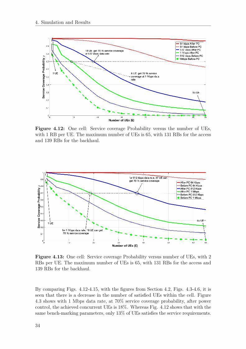
4. Simulation and Results
Figure 4.12: One cell: Service coverage Probability versus the number of UEs,with 1 RB per UE. The maximum number of UEs is 65, with 131 RBs for the accessand 139 RBs for the backhaul.
Figure 4.13: One cell: Service coverage Probability versus number of UEs, with 2RBs per UE. The maximum number of UEs is 65, with 131 RBs for the access and139 RBs for the backhaul.
By comparing Figs. 4.12-4.15, with the figures from Section 4.2, Figs. 4.3-4.6, it isseen that there is a decrease in the number of satisfied UEs within the cell. Figure4.3 shows with 1 Mbps data rate, at 70% service coverage probability, after powercontrol, the achieved concurrent UEs is 18%. Whereas Fig. 4.12 shows that with thesame bench-marking parameters, only 13% of UEs satisfies the service requirements.
34

4. Simulation and Results
Figure 4.14: One cell: Service coverage Probability versus the number of UEs,with 3 RBs per UE. The maximum number of UEs is 43, with 131 RBs for theaccess and 139 RBs for the backhaul.
Figure 4.15: One cell: Service coverage Probability versus the number of UEs,with 4 RBs per UE. The maximum number of UEs is 32, with 131 RBs for theaccess and 139 RBs for the backhaul.
Evidently, an increase in the number of concurrent UEs transmitting within a cellleads to a gradual decrease in the service coverage probability. For instance, com-paring Fig. 4.4 with Fig. 4.13, it is seen that in Fig. 4.4 with 512 kbps baseline datarate, at 70% service coverage after power control, the achievable concurrent UEs is60%, while in Fig. 4.13, with 512 kbps baseline data rate, at 70% service coverage
35

4. Simulation and Results
after power control, the achievable concurrent UEs is 57%. Also, Fig. 4.5 showsthat with 3 Mbps baseline rate, at 70% service coverage after power control, theachievable concurrent UEs is 28%, while in Fig. 4.14, with the same baseline, shows20% of UEs can satisfy the service requirement at 70% service coverage probability.The observation may be attributed to the fact that the interference power that eachUEi has to contend with is increasing, as well as the interference between the accessand backhaul links in TDD.
Moreover, the advantage of separating the access and backhaul links in TDD isseen in all test cases as the service coverage probability, before and after powercontrol, is higher in Section 4.2 than when they operate simultaneously in this testcase. Although, with 64 kbps as the minimum data rate, there seem to be no differ-ence. The unnoticeable difference may be attributed to a low data rate and SINRrequirement which is needed for UE control or signaling within the IAB network.Generally, in TDD profile, there are RBs used for synchronization between the trans-mitter and the receiver, [7]. The synchronization creates guard time between the ULand DL thereby guaranteeing a stable communication system and reducing interfer-ence. Without proper synchronization, simultaneous transmission in TDD reducesthe signal quality. The results from these test cases points to this fact, that overlapin RBs due to simultaneous UL and DL reduces the service coverage probability.
4.5 Effect of Interference on Simultaneous Accessand Backhaul Links (Two Cells)
The set-up during this test consists of two adjacent MBS cells where the access andbackhaul links are operating simultaneously. The SBSs and the UEs associated withthe MBS are the only entities transmitting at the same time.
Interference occurs between the UEs associated with the MBS and all the SBSs.The number of UEs associated with the MBS is a fraction of the total number ofUEs randomly placed in the cell. There is a possibility of the UEs transmittingmore power to overcome the interference from the SBSs, whose minimum transmitpower is 35 dBm. Also, this set-up investigates the effect of inter-cell interference onservice coverage probability with simultaneous operation of the access and backhaullinks. The results of the test cases are shown in Figs. 4.16-4.19.
In all cases, the cell radius in each cell is fixed. The varying parameters are thedata rates, number of concurrent UEs and the RBs per UE. The set-up cell coverageis modeled as a hexagon avoiding overlap from the other cell. The random distri-bution of the UEs provides the possibility of having UEs located at the edge of thecells, thereby contributing to inter-cell interference.
36

4. Simulation and Results
Figure 4.16: Two cell: Service coverage probability versus the number of UEs,with 1 RB per UE. The maximum number of UEs is 65, with 131 RBs for the accessand 139 RBs for the backhaul.
Here, it is observed that the number of satisfied UEs is at the lowest comparedwith other scenarios and test cases. The observation may be due to increase in theinterference power that the UEs are contending with. The set-up has both intra-celland inter-cell interference at the same time. The combined interference may explainwhy the results here offer the lowest service coverage probability when comparedwith other simulations.
Figure 4.17: Two cell: Service coverage probability versus the number of UEs,with 2 RBs per UE. The maximum number of UEs is 65.
37
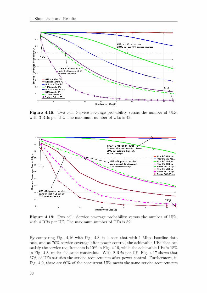
4. Simulation and Results
Figure 4.18: Two cell: Service coverage probability versus the number of UEs,with 3 RBs per UE. The maximum number of UEs is 43.
Figure 4.19: Two cell: Service coverage probability versus the number of UEs,with 4 RBs per UE. The maximum number of UEs is 32.
By comparing Fig. 4.16 with Fig. 4.8, it is seen that with 1 Mbps baseline datarate, and at 70% service coverage after power control, the achievable UEs that cansatisfy the service requirements is 10% in Fig. 4.16, while the achievable UEs is 18%in Fig. 4.8, under the same constraints. With 2 RBs per UE, Fig. 4.17 shows that57% of UEs satisfies the service requirements after power control. Furthermore, inFig. 4.9, there are 60% of the concurrent UEs meets the same service requirements
38

4. Simulation and Results
after power control. Then, Fig. 4.11 shows that 40% of the concurrent UEs with3 Mbps baseline data rate, meets the service requirements at 70% service coverageprobability after power control, versus in Fig. 4.19, which shows that 36% of theconcurrent UEs meets the service requirements at 70% service coverage probabilityafter power control.
Here, the increase in the interference power affects the access and backhaul linksworking at the same time. Without proper separation between the RBs used in theaccess and backhaul links, the service quality may reduce. The decrease in servicequality reflects in the number of UEs actively within the cell and the decrease inservice coverage probability. Also, having high performing backhaul links is impor-tant for the RAN. If the performance of the backhaul links is low, it reflects in theperformance of the access links as well.
4.6 Data Rate Analysis for the UEs
Based on the Eq. (3.21), the achievable data rates per UE is being observed. Build-ing on the results from Sections 4.2 and 4.4, Figs. 4.20-4.23 are generated. Thefigures compares the actual UE data rates after power control versus the servicecoverage probability. The analysis is done for cases with 1 RB per UE and 4 RBsper UE. The investigation is looking at the average guaranteed data rate per UE,with and without power control, given a number of concurrent UEs within the set-up.
Figure 4.20: One cell: Service coverage probability versus the data rate with 1 RBper UE, Rb = 1 Mbps. The analysis is for the data rate values after power control.
39
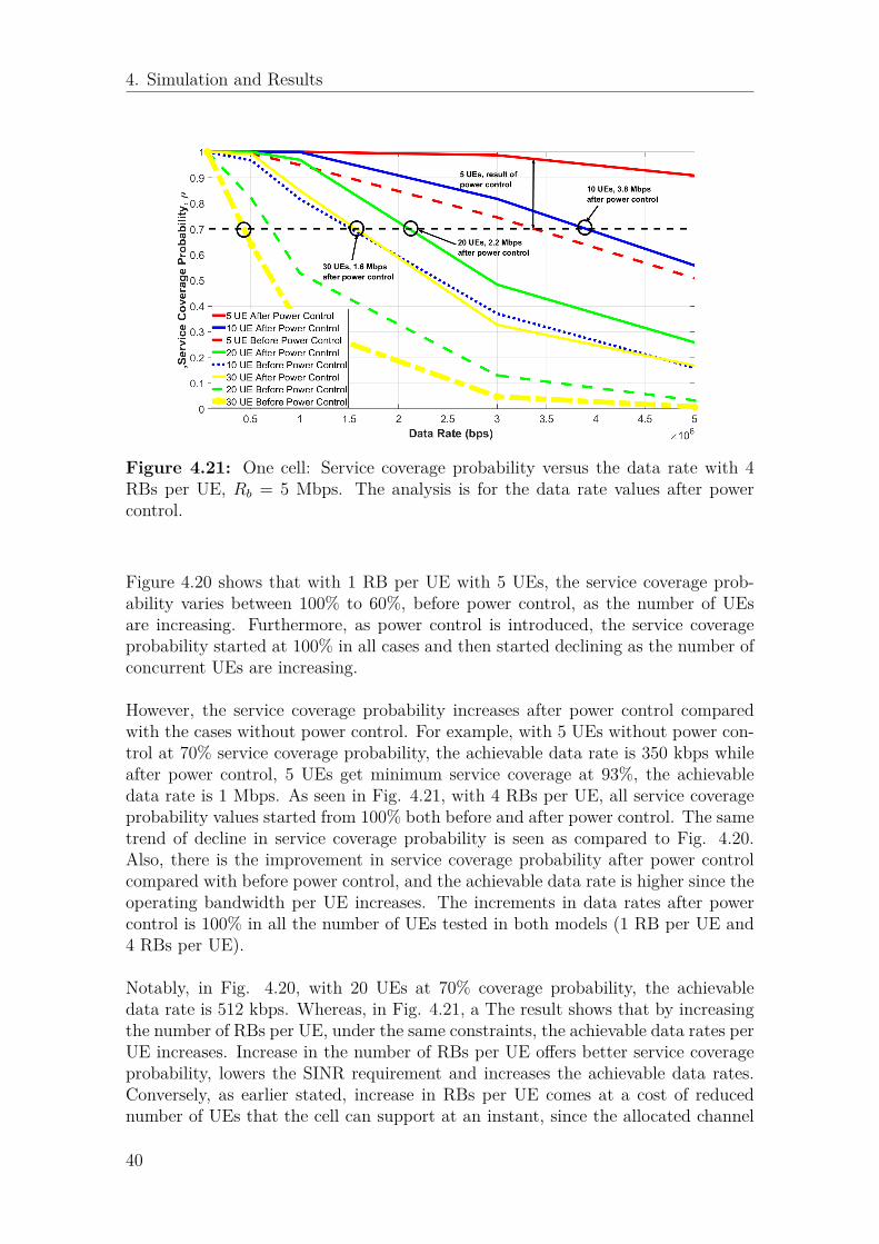
4. Simulation and Results
Figure 4.21: One cell: Service coverage probability versus the data rate with 4RBs per UE, Rb = 5 Mbps. The analysis is for the data rate values after powercontrol.
Figure 4.20 shows that with 1 RB per UE with 5 UEs, the service coverage prob-ability varies between 100% to 60%, before power control, as the number of UEsare increasing. Furthermore, as power control is introduced, the service coverageprobability started at 100% in all cases and then started declining as the number ofconcurrent UEs are increasing.
However, the service coverage probability increases after power control comparedwith the cases without power control. For example, with 5 UEs without power con-trol at 70% service coverage probability, the achievable data rate is 350 kbps whileafter power control, 5 UEs get minimum service coverage at 93%, the achievabledata rate is 1 Mbps. As seen in Fig. 4.21, with 4 RBs per UE, all service coverageprobability values started from 100% both before and after power control. The sametrend of decline in service coverage probability is seen as compared to Fig. 4.20.Also, there is the improvement in service coverage probability after power controlcompared with before power control, and the achievable data rate is higher since theoperating bandwidth per UE increases. The increments in data rates after powercontrol is 100% in all the number of UEs tested in both models (1 RB per UE and4 RBs per UE).
Notably, in Fig. 4.20, with 20 UEs at 70% coverage probability, the achievabledata rate is 512 kbps. Whereas, in Fig. 4.21, a The result shows that by increasingthe number of RBs per UE, under the same constraints, the achievable data rates perUE increases. Increase in the number of RBs per UE offers better service coverageprobability, lowers the SINR requirement and increases the achievable data rates.Conversely, as earlier stated, increase in RBs per UE comes at a cost of reducednumber of UEs that the cell can support at an instant, since the allocated channel
40

4. Simulation and Results
bandwidth is fixed.
Figure 4.22: One cell special case: Service coverage probability versus the datarate with 1 RB per UE, Rb = 1 Mbps. The analysis is for the data rate values afterpower control.
Figure 4.23: One cell special case: Service coverage probability versus the datarate with 4 RBs per UE, Rb = 5 Mbps. The analysis is for the data rate values afterpower control.
Also, comparing Fig. 4.21 with Fig. 4.23, the results show the same trend just as
41

4. Simulation and Results
in Fig. 4.20 and Fig. 4.21. As the number of RB per UE increases, the achievabledata rate and service coverage probability increases. Interestingly, from Fig. 4.20with 20 UEs at 70% coverage probability after power control, the achievable datarate 512 kbps, while from Fig. 4.22 with 20 UEs at 70% coverage probability afterpower control offers achievable data rate of 430 kbps. Also, with 60 UEs at 70%coverage probability after power control, 250 kbps is the achievable data rate inboth Fig. 4.20 and Fig. 4.22. Since there is only 1 RB per UE, there is a higherSINR requirement, with higher transmit power requirement, which builds up theinterference signal.Moreover, from Fig. 4.21, with 10 UEs at 70% service coverage after power control,the achievable data rate is 3.8 Mbps, while with 20 UEs at the same benchmark,the achievable data rate is 2.2 Mbps. Conversely, Fig. 4.23 shows that with 20 UEsat 70% service coverage after power control, the achievable data rate is 2 Mbps andwith 10 UEs at 70% service coverage after power control, the achievable data rateis 3.3 Mbps. Although, the RBs per UE is 4 and the SINR requirement is muchlower, the interference between the access and backhaul links limits the achievabledata rates. The interference is expected to scale up as the number of concurrentUEs within the cell increases.
4.7 Comparison between IAB and non-IAB Net-work
In Fig. 4.24, we show the service coverage probability for a non-IAB network, i.e.,the cases with no SBS. Here, the results are presented for the cases with 4 RBs perUE with varying baseline data rates.
Figure 4.24: One cell: Service coverage probability versus the number of UEs,with 4 RB per UE, E =32, in non-IAB network.
42

4. Simulation and Results
Here, the result is compared with Fig. 4.6. The comparison shows that there isa possibility of having better service coverage probability with IAB networks thanwith non-IAB networks. From Fig. 4.24, at 70% service coverage probability with 3Mbps baseline data rate, only 3 UEs are satisfied, versus 13 UEs, as seen in Fig. 4.6,after power control. Also, a steady decline in service coverage probability startedjust after the first UE is introduced into the cell in Fig. 4.24, while a decline startedafter 6 UEs are introduced randomly into the cell, for the same baseline data rateof 3 Mbps after power control in Fig. 4.6.
Interestingly, considering 3 Mbps as the baseline data rate, it is observed that with25 UEs, before and after power control gives a zero service coverage probabilityfor the non-IAB network. Meanwhile, with the modeled IAB network, the servicecoverage probability with 25 UEs, after power control, is about 40%. Thus, a well-planned and deployed IAB networks, with power control, may offer a better servicecoverage, compared to non-IAB networks.
4.8 Determination of the Effective Cell RadiusOne of the parameters being optimized in IAB networks is the service coverage area.The service coverage area is directly related to the cell radius of the MBS. Our modelis initially built on a cell radius of 200 m. In this test case, the cell radius is increasedstep-wise to 700 m. The simulation tries to observe the radius of the cell at whichthe service coverage probability starts to decline or shows a flat profile. Figure 4.25shows the results.
Figure 4.25: One cell: Service coverage probability versus increasing cell radius,with 4 RBs per UE, from 200 m to 700 m (E = 32).
The results show that before power control, there was a slight increase in the ser-vice coverage probability. The slight increase may be attributed to a reduction in
43

4. Simulation and Results
interference between UEs as the distance between the UEs increases, since there isa fixed number of UEs within the cell and they transmit at the same power of 23dBm. With 64 kbps baseline data rate, both before and after power control, withincreasing cell radius, the service coverage probability is the same. Furthermore, itis observed that by increasing the radius from 300 m to 400 m, the service coverageprobability starts to decline and flatten out in other test cases. The observationmay relate to the fact that the UEs at the edge of the cell are already transmittingat their maximum allowed transmit power and cannot do more than 43 dBm atthis point. Knowing that the model uses mmWave which has short wavelength andshort effective distance, it is seen that the service coverage probability within thecell starts to decrease after power control at around 300 m cell radius, for the samenumber of UEs randomly distributed.Furthermore, the results from other tests related to inter-cell interference with twoadjacent cells can be found in the appendix of our report, Appendix A. The resultsare other investigations about intra-cell and inter-cell interference in IAB networks.
4.9 Transmit Power Distribution of UEsHere, the transmit power distribution of the UEs are analyzed. The cumulativedistribution function (CDF) plot of the transmit powers shows the continuous dis-tribution of the transmit powers for the UEs associated with the SBSs and the UEsassociated with the MBS from a test case in Section 4.2. The CDF plot also showsthe percentage of transmit power values of the UEs depending on the baseline servicerequirements. The CDF values range from the minimum to the maximum transmitpowers proposed by 3GPP, [28].
Figure 4.26: CDF for UEs associated with the SBS with fixed cell radius. Theanalysis is for the distribution of the transmit power values after power control.
44

4. Simulation and Results
From Fig. 4.26, derived from same data used in Section 4.2, it is observed that thedistribution of the transmit powers reaches the CDF peaks between 35 dBm and 39dBm. Here, there are 4 RBs allocated to each UE, with maximum of 32 concurrentUEs within the cell. Given a baseline of 1 Mbps, the transmit power peak startsfrom 39 dBm, which is the highest in all the test cases. Meanwhile, for lower datarates, 64 kbps and 512 kbps, the CDF peaks are at 35 dBm with lower distributionof transmit powers. Then, for 3 Mbps and 5 Mbps, have distribution more from 32dBm to 36 dBm. As earlier established, the higher the data rate requirement, thehigher the SINR requirement as well. For the UEs to have higher data rates, theyneed more transmit power and still need to operate with minimal interference.
From Eq.(3.12), it is obvious that data rate, Rb, and SINR have a linear relation-ship, given a fixed bandwidth. Therefore, higher baseline data rate results in higherSINR requirement and more transmit power as well. With higher transmit powerfrom the UEs, the interference within the cell increases and the service coverageprobability reduces, meaning some UEs cannot meet the service requirements. Thenumber of satisfied UEs reduces and the instant transmit power of the remainingsatisfied UEs may reduce as well due to the GA final solutions, because interferencewill also reduce as some UEs dropped off. The change in power level and reducednumber of UEs may be the reason why with 1 Mbps baseline data rate, there is ahigher power distribution than with 3 Mbps or 5 Mbps test cases. Invariably, thenumber of satisfied UEs are more with 1 Mbps baseline data rate than with 3 Mbpsand 5 Mbps test cases.
Figure 4.27: CDF for UEs associated with the MBS with fixed cell radius. Theanalysis is for the distribution of the transmit power values after power control.
From Fig. 4.27, it is observed that for the UEs associated with the MBS, the trans-mit power distribution is similar to what is seen in Fig. 4.26. Although, taking alook at 1 Mbps baseline data rate, the CDF reaches a peak at 38 dBm, which is 1
45

4. Simulation and Results
dBm less than the CDF of UEs associated with the SBS. There is a possibility ofhaving more UEs associated with the SBS than with the MBS, which may increasethe interference at the SBS. Then, the UEs transmit more power to meet the SINRrequirement and to overcome the interference from other UEs.
Generally, comparing Fig. 4.26 and Fig. 4.27, it is observed that there is relativelythe same transmit power distribution of all the UEs irrespective of their associatedBS, either MBS or SBS, after power control. The results may point to the fact thatpower control tries to create a transmit power balance across all UEs within a cell,thereby improving the network capacity.
4.10 Convergence of the Genetic AlgorithmIn all simulations, GA is used as a central daemon to offer fair power allocation valuesto the respective UEs and SBSs in uplink communication. The GA converged in allcases but at different iteration counts. Figure 4.28 shows the convergence of the GAfrom three simulations.
Figure 4.28: Plots of the convergence of Genetic Algorithm. Different GA conver-gence plots are captured for different simulations.
Specifically, as detailed in the Algorithm, we set N = 200, K = 20 and S = 10.As seen in Fig. 4.28, the algorithm converges in a ladder form. The observed lad-der form is because using GA is not necessarily to find the best solution in everyiteration, and it may be trapped in a local minimum. However, due to Step 4 andStep 6 of the Algorithm, GA can always avoid a local minimal and reach the globaloptimum if a sufficiently large number of iteration is considered, [39]- [42]. In GA,the larger the value of N , the more accurate the final solutions but at a cost ofthe iteration time. The higher the value of N , the slower the time taken for thealgorithm to offer proper final solutions. Mostly, there is a trade-off between speed
46

4. Simulation and Results
and accuracy in iterative algorithms.
Also, it should be noted that the GA is independent of the channel model andso it can be applied in different channel models, [39]- [42]. From the results pro-vided in our work, the GA offered a power control solution which could improve theservice coverage probability of IAB networks. In all test cases, GA offers reasonablesolutions for our multi-objective problem formulation.
47

5Conclusion
This work investigated the performance of an IAB network using 3GPP proposedparameters. Particularly, we studied the effect of uplink power control on the servicecoverage probability of two-hop IAB network. For this reason, we developed a GA-based scheme for power control, and studied the effect of different parameters on thenetwork performance. Our work considered a 28 GHz band for 5G deployment withTDD. We considered a finite number of resource blocks that a BS can offer in 5G.The model set-up had a cell radius of 200 m from the MBS. The UEs were randomlydistributed per iteration to mimic the mobility. The pathloss was modeled using the3GPP UMa model, putting into consideration the height of a MBS, SBSs, and UEsrespectively. Also, fading, shadowing, and effects of rain were added to the overallchannel loss. The EIRP values of the UE transmit power, as suggested by 3GPP,were used in the simulations. The baseline received SINR value was set to guaranteea target uplink data rate and assumed uncoded transmission. The power controlsolution was based on GA, implemented as a central daemon in the RAN. Signalinterference seems to be a challenge that may limit the service coverage probabilityof IAB networks.Based on the simulations carried out and our further analysis, it is observed thatfor effective control and minimization of interference, in TDD context, there shouldbe a separation in time between the access and backhaul links. Without this, thereis a possibility to increase the interference within the cell to an extent that the UEswill not have enough transmit power again to overcome the signal interference for agiven baseline service requirement.Moreover, with an increase in the allocated RBs per UE, or the UE operating band-width, there is a high possibility for better service coverage probability and higherdata rates, at a cost of reduced number of concurrent UEs. Based on our models,the effect of inter-cell interference is minimal with a MBS cell of > 200 m radius,operating at 28 GHz band, and channel bandwidth of 400 MHz. It is observed that,for the considered parameter setting, the effective cell radius is in between 300 m to400 m.Interestingly, the GA gives a proper power control to the transmit signal in termsof fairness and speed as an iterative power allocation scheme, which usually needsmore time to converge. In most cases, the GA converges in less than 50 iterations.As demonstrated in all cases, a well-designed and implemented uplink power con-trol scheme may improve service coverage probability in some cases within the IABnetworks. Also, there is a possibility of having a better service quality with IABnetworks as compared to non-IAB networks.
48

6Future Works
Interestingly, the thesis work studied uplink power control in 5G IAB network undersome defined conditions. It offers some logical conclusions into what must be putinto perspective when deploying a 5G IAB network with the wireless channel band-width being shared between the access and backhaul links. Furthermore, the workalso gives insight into some other areas that should be considered for future works,which will eventually lead to an all-encompassing IAB network solution. These in-cludes:
• Identify a workable solution for load-balancing the UEs or traffic within an IABnetwork. Preferably, some IAB nodes, or BSs, should have a high cell load whileothers have less, based on the instantaneous quality of the backhaul links and thenumber of associated UEs. Having an appropriate distribution of the traffic loadacross all the BSs will help to avoid backhaul congestion.• Investigate on combining power control and rate adaptation in the IAB uplinkcommunication. The work may give insight into the variations of data rates thatthe UEs can have in uplink communication.• Investigate the effect of edge computing and data storage capability of the IABnodes on the QoS and QoE of the UEs.• Identify and compare different efficient algorithms for resource allocation, includ-ing distributed power control schemes.• Modelling massive MIMO for MBSs and SBSs, with beamforming capability, inuplink communication.• Investigate the use of digital coding techniques in the massive MIMO use casesto control, or reduce, the effect of signal interference.
49

6. Future Works
50

Bibliography
[1] V. Sahin, C. G. Omidyar and T. M. Bauman, "Telecommunications manage-ment network (TMN) architecture and interworking designs," in IEEE Journalon Selected Areas in Communications, vol. 6, no. 4, pp. 685-696, May 1988.
[2] K.Flynn, 2020. 5G for Industry 4.0. [online] 3gpp.org. Available at:https://www.3gpp.org/news-events/2122-tsn_v_lan [Accessed 5 June 2021].
[3] Y. Yang, K. W. Sung, L. Wosinska and J. Chen, "Hybrid fiber and microwaveprotection for mobile backhauling," in IEEE Wireless Commun. Lett./OSAJournal of Optical Communications and Networking, vol. 6, no. 10, pp. 869-878,Oct. 2014.
[4] L. Ma, X. Wen, L. Wang, Z. Lu and R. Knopp, "An SDN/NFV based frameworkfor management and deployment of service based 5G core network," in ChinaCommunications, vol. 15, no. 10, pp. 86-98, Oct. 2018.
[5] S. Ahmadi, 2019. 5G NR. 1st ed. London: Academic Press, Elsevier Inc., pp.1- 56, 254, 371-373, 380-400.
[6] Ericsson. Mobile Data Traffic Growth Outlook. Accessed: Jun. 5, 2021.[Online]. Available: https://www.ericsson.com/491e34/assets/local/mobility-report/documents/2018/ericsson-mobility-report-november-2018.pdf
[7] A. Goldsmith, 2005. Wireless communications. Cambridge: Cambridge Univer-sity Press, pp.77-78, 293-315, 466-494, 505-528.
[8] S. Sreekumar, B. K. Dey and S. R. B. Pillai, "Distributed rate adaptation andpower control in fading multiple access channels," in IEEE Trans. Inf. Theory,vol. 61, no. 10, pp. 5504-5524, Oct. 2015.
[9] C. Madapatha, 2020. Integrated access and backhaul for 5G and beyond. Mas-ter’s Thesis. [online] Gothenburg: Chalmers University of Technology, pp.5-24.
[10] C. Madapatha, B. Makki, C. Fang, O. Teyeb, E. Dahlman, M. Alouini, T.Svensson. "On integrated access and backhaul networks: current status andpotentials," in IEEE Open Journal of the Communications Society, vol. 1, pp.1374-1389, 2020.
[11] M. Polese, M. Giordani, A. Roy, S. Goyal, D. Castor and M. Zorzi, "End-to-End simulation of integrated access and backhaul at mmWaves," in Proc. IEEECAMAD’2018, Barcelona, Spain, 2018, pp. 1-7.
[12] A. Łukowa, V. Venkatasubramanian, E. Visotsky and M. Cudak, "On the cov-erage extension of 5G millimeter wave deployments using integrated access andbackhaul," in Proc. IEEE PIMRC’2020, London, United Kingdom, 2020, pp.1-7.
51

Bibliography
[13] E. Lagunas, L. Lei, S. Maleki, S. Chatzinotas and B. Ottersten, "Power al-location for in-band full-duplex self-backhauling," in Proc. IEEE TSP’2017,Barcelona, Spain, 2017, pp. 136-139.
[14] O. Teyeb, A. Muhammad, G. Mildh, E. Dahlman, F. Barac and B. Makki,"Integrated access backhauled Networks," in Proc. IEEE VTC’2019, Honolulu,HI, USA, 2019, pp. 1-5.
[15] M. Gupta, A. Rao, E. Visotsky, A. Ghosh and J. G. Andrews, "Learning linkschedules in self-backhauled millimeter wave cellular networks," in IEEE Trans-actions on Wireless Communications, vol. 19, no. 12, pp. 8024-8038, Dec. 2020.
[16] C. Madapatha, B. Makki, A. Muhammad, E. Dahlman, M. Alouini,T.Svensson, "On topology optimization and routing in integratedaccess and backhaul networks: A Genetic Algorithm-based Ap-proach", arXiv preprint arXiv:2102.07252, Feb. 2021. [Online]. Available:https://arxiv.org/pdf/2102.07252.pdf.
[17] H. Guo, B. Makki, D. Phan-Huy, E. Dahlman, M. Alouini, T. Svens-son., “Predictor Antenna: A Technique to Boost the Performance of Mov-ing Relays”, arXiv preprint arXiv:2012.10537, May 2021.[Online]. Available:https://arxiv.org/pdf/2012.10537.pdf
[18] C. Fang, C. Madapatha, B. Makki, T.Svensson, "Joint scheduling andthroughput maximization in self-backhauled millimeter wave cellular net-works", arXiv preprint arXiv:2106.02570, Jun. 2021. [Online]. Available:https://arxiv.org/pdf/2106.02570.pdf.
[19] T. Inoue, "5G NR Release 16 and millimeter wave integrated access and back-haul," 2020 IEEE Radio and Wireless Symposium (RWS), San Antonio, TX,USA, 2020, pp. 56-59.
[20] GSMA, 2019. 5G Implementation Guidelines. [online] Gsma.com. Availableat: https://www.gsma.com/futurenetworks/wp-content/uploads/2019/03/5G-Implementation-Guideline-v2.0-July-2019.pdf. pp.16-18.
[21] S. Nagul, "A review on 5G modulation schemes and their comparisons for futurewireless communications," in Proc. IEEE SPACES’2018, Vijayawada, India,2018, pp. 72-76.
[22] J. Navarro-Ortiz, P. Romero-Diaz, S. Sendra, P. Ameigeiras, J. J. Ramos-Munozand J. M. Lopez-Soler, "A survey on 5G usage scenarios and traffic models," inIEEE Communications Surveys Tutorials, vol. 22, no. 2, pp. 905-929, Secondquarter 2020.
[23] Y. Takahashi, K. Muraoka, J. Mashino, S. Suyama and Y. Okumura, "5GDownlink throughput performance of 28 GHz band experimental trial at 300km/h," in Proc. IEEE PIMRC’2018, pp. 1140-1141.
[24] R. Tian, K. Senda and H. Otsuka, "BER performance of OFDM-based 4096-QAM using soft decision Viterbi decoding in multipath fading," in Proc. IEEEWSCE’2018, Singapore, pp. 1-4.
[25] M. N. Islam, S. Subramanian and A. Sampath, "Integrated access backhaul inmillimeter wave networks," in Proc. IEEE WCNC, 2017, pp. 1-6.
[26] A. Zaidi, F. Athley, J. Medbo, U. Gustavsson, G. Durisi, and X. Chen, 2018.5G physical layer. 1st ed. London: Academic Press, pp.23-64.
52

Bibliography
[27] G. Barb, M. Otesteanu, F. Alexa and F. Danuti, "OFDM multi-numerology forfuture 5G New Radio communication systems," in Proc. IEEE SoftCOM’2020,Split, Croatia, 2020, pp. 1-3.
[28] 3GPP TS 38.101-2 V17.1.0 (2021-03) NR;User Equipment (UE) radio trans-mission and reception; Part 2: Range 2 Standalone (Release 17). Available at:https://www.3gpp.org/ftp/Specs/archive/38_series/38.101-2/
[29] Nokia, 2020. Looking for faster 5G mmWave rollout?. [image] Avail-able at: https://www.nokia.com/blog/looking-for-faster-5g-mmwave-rollout-find-out-how-iab-will-help/
[30] J. Kim, I. Kim and H. Chung, "Resource multiplexing enhancements for in-tegrated access and backhaul in 5G New Radio Release 17," in Proc. IEEEICTC’2020, pp. 936-938.
[31] H. Ronkainen, J. Edstam, A. Ericsson, and C. Östberg, 2020. In-troducing Integrated Access and Backhaul. Ericsson Technology Re-view, [online] (ISSN 0014-0171 284 23-3346), pp.4-7. Available at:https://www.ericsson.com/49e6f6/assets/local/reports-papers/ericsson-technology-review/docs/2020/introducing-integrated-access-and-backhaul.pdf
[32] R. Dilli, "Analysis of 5G wireless systems in FR1 and FR2 frequency bands,"in Proc. IEEE ICIMIA’2020, pp. 767-772.
[33] 3GPP TR 38.901 V16.1.0 (2019-12) Study on channel modelfor frequencies from 0.5 to 100 GHz (Release 16). Availableat:https://www.3gpp.org/ftp/Specs/archive/38_series/38.901/
[34] J. Huang, Y. Cao, X. Raimundo, A. Cheema and S. Salous, "Rain statisticsinvestigation and rain attenuation modeling for millimeter wave short-rangefixed links," in IEEE Access, vol. 7, pp. 156110-156120, 2019.
[35] ITU-R Recommendation P.838-3. ‘Specific attenuation model for rain foruse in prediction methods’, International Telecommunication Union, 2006.Available at: https://www.itu.int/dms_pubrec/itu-r/rec/p/R-REC-P.838-3-200503-I!!PDF-E.pdf
[36] 3GPP TS 38.300 V16.2.0 (2020-07) Technical Specification Group Radio Ac-cess Network;NR; NR and NG-RAN Overall Description;Stage 2(Release 16).Available at:https://www.3gpp.org/ftp/Specs/archive/38_series/38.300/
[37] K. Ulaganathen, A. R. Tharek, R. M. Islam and K. Abdullah, "Rain attenuationfor 5G network in tropical region (Malaysia) for terrestrial link,"in Proc. IEEEMICC’2017, pp. 35-38.
[38] G. R. MacCartney and T. S. Rappaport, "Millimeter-wave base station diversityfor 5G coordinated multipoint (CoMP) applications," in IEEE Transactions onWireless Communications, vol. 18, no. 7, pp. 3395-3410, July 2019.
[39] B. Makki, A. Ide, T. Svensson, T. Eriksson and M. Alouini, "A geneticalgorithm-based antenna selection approach for large-but-finite MIMO net-works," in IEEE Transactions on Vehicular Technology, vol. 66, no. 7, pp.6591-6595, July 2017.
[40] B. Makki, T. Svensson and M. Alouini, "On the throughput of large-but-finiteMIMO networks using schedulers," in IEEE Trans. Wireless Commun., vol. 18,no. 1, pp. 152-166, Jan. 2019.
53

Bibliography
[41] H. Guo, B. Makki and T. Svensson, "A genetic algorithm-based beamformingapproach for delay-constrained networks," in Proc. IEEE WiOpt’2017, pp. 1-7.
[42] B. Makki, T. Svensson, G. Cocco, T. de Cola and S. Erl, "On the throughputof the return-link multi-beam satellite systems using genetic algorithm-basedschedulers," in Proc. IEEE ICC’2015, pp. 838-843.
54

AAppendix 1
A.1 Inter-cell Distance and Inter-cell InterferenceBy increasing the inter-cell distance, we may observe some effects of inter-cell in-terference. This set-up shows only about 1% improvement in the service coverageprobability, after power control. Empirically, it is taken therefore that the interfer-ence from adjacent cells is quite minimal. This is inferred from figure A.1.
Note: The operating frequency band is 28 GHz with a cell radius of 200 m and 32UEs only.
Figure A.1: Service coverage probability versus inter-cell distance. Here, only twoadjacent cells are used for the test, the distance between two cells start for 0 to 200m, E = 4, RB = 2 per UE, E = 32.
A.2 Intra-cell Distance and Intra-cell InterferenceAlso, by increasing the cell radius, we may observe a trend in the service coverageprobability. It is observed that the service coverage probability, after power control,starts to decline at distances between 300 m and 400 m, depending on the baselinedata rate and RB.
I

A. Appendix 1
Figure A.2: Service coverage probability versus intra-cell distance, r = (200 m to700 m), with 1 RB per UE, E = 32, M = 4.
Figure A.3: Service coverage probability versus intra-cell distance, r = (200 m to700 m), with 2 RBs per UE, E = 32, M = 4 .
II

DEPARTMENT OF SOME SUBJECT OR TECHNOLOGYCHALMERS UNIVERSITY OF TECHNOLOGYGothenburg, Swedenwww.chalmers.se